Grids of stellar models with rotation

arX

iv:1

203.

5243

v2 [

astr

o-ph

.SR

] 24

Apr

201

2Astronomy & Astrophysicsmanuscript no. WRPopulations˙Corrected c© ESO 2018November 7, 2018

Grids of stellar models with rotationII. WR populations and supernovae/GRB progenitors at Z = 0.014

C. Georgy1, S. Ekstrom2, G. Meynet2, P. Massey3, E. M. Levesque4, R. Hirschi5,6, P. Eggenberger2, A. Maeder2

1 Centre de Recherche Astrophysique de Lyon, Ecole Normale Superieure de Lyon, 46, allee d’Italie, F-69384 Lyon cedex 07, France2 Geneva Observatory, University of Geneva, Maillettes 51, CH-1290 Sauverny, Switzerland3 Lowell Observatory, 1400 W Mars Hill Road, Flagstaff, AZ 86001, USA4 CASA, Department of Astrophysical and Planetary Sciences,University of Colorado 389-UCB, Boulder, CO 80309, USA5 Astrophysics group, EPSAM, Keele University, Lennard-Jones Labs, Keele, ST5 5BG, UK6 Institute for the Physics and Mathematics of the Universe, University of Tokyo, 5-1-5 Kashiwanoha, Kashiwa, 277-8583,Japan

Received ; accepted

ABSTRACT

Context. In recent years, many very interesting observations have appeared concerning the positions of Wolf-Rayet (WR) stars intheHertzsprung-Russell diagram (HRD), the number ratios of WRstars, the nature of type Ibc supernova (SN) progenitors, long and softgamma ray bursts (LGRB), and the frequency of these various types of explosive events. These observations represent keyconstraintson massive star evolution.Aims. We study, in the framework of the single-star evolutionary scenario, how rotation modifies the evolution of a given initial massstar towards the WR phase and how it impacts the rates of type Ibc SNe. We also discuss the initial conditions required to obtaincollapsars and LGRB.Methods. We used a recent grid of stellar models computed with and without rotation to make predictions concerning the WRpopulations and the frequency of different types of core-collapse SNe. Current rotating models were checked to provide good fitsto the following features: solar luminosity and radius at the solar age, main-sequence width, red-giant and red-supergiant (RSG)positions in the HRD, surface abundances, and rotational velocities.Results. Rotating stellar models predict that about half of the observed WR stars and at least half of the type Ibc SNe may be producedthrough the single-star evolution channel. Rotation increases the duration of the WNL and WNC phases, while reducing those of theWNE and WC phases, as was already shown in previous works. Rotation increases the frequency of type Ic SNe. The upper mass limitfor type II-P SNe is∼ 19.0 M⊙ for the non rotating models and∼ 16.8 M⊙ for the rotating ones. Both values agree with observations.Moreover, present rotating models provide a very good fit to the progenitor of SN 2008ax. We discuss future directions of researchfor further improving the agreement between the models and the observations. We conclude that the mass-loss rates in theWNL andRSG phases are probably underestimated at present. We show that up to an initial mass of 40M⊙, a surface magnetic field inferior toabout 200 G may be sufficient to produce some braking. Much lower values are needed at the red supergiant stage. We suggest thatthe presence/absence of any magnetic braking effect may play a key role in questions regarding rotation ratesof young pulsars andthe evolution leading to LGRBs.

Key words. stars: general – stars: evolution – stars: rotation – stars:Wolf-Rayet – supernovae: general

1. Introduction

Wolf-Rayet (WR) stars are characterised by four importantobserved features (see the recent reviews by Massey 2003;Crowther 2007):

1. They are associated with young massive star regions.2. They present broad and strong emission lines.3. They are hot (log(Teff/K) & 4) and luminous stars

(log(L/L⊙) > 5.0).4. The chemical composition of their surface shows signs of

H-burning (WN-type) and/or He-burning processes (WNC,WC, WO-type).

These features can be satisfactorily explained if WR are mas-sive evolved stars whose surface composition has been changedby mass loss and/or internal mixing. The mass loss can be dueeither to stellar winds and/or to the loss of the envelope througha Roche lobe overflow (RLOF) in a close-binary system.

The estimated total number of WR stars in the Milky Way isabout 6000–6500 (Shara et al. 2009). It means that about 1 outof

20 million stars is a WR star in the Galaxy. To date, 476 galacticWR stars have been detected,i.e. about 7–8% of the total MilkyWay population (Mauerhan et al. 2011). Although these starsarequite rare, they are important in astrophysics for many reasons:

– They represent an evolved state of the most massive stars(seee.g. Schnurr et al. 2008; Rauw et al. 2004; Lamers et al.1991).

– They allow us to check the nuclear reaction chains during theH- and He-burning phases (seee.g. Dessart et al. 2000).

– They suffer strong mass loss, making them very inter-esting laboratories for studying the physics of stellarwinds. Many of them are surrounded by extended nebulae(Stock & Barlow 2010).

– They are candidate progenitors for type Ibc supernovae(SNe)1, which give birth to either a neutron star (NS) or ablack hole (BH, Smartt 2009).

1 In this paper, we call the sample composed of type Ib and type IcSNe type Ibc SNe.

1

http://arxiv.org/abs/1203.5243v2

Georgy et al.: Grids of stellar models with rotation

– They may be the progenitors of long and soft gamma-raybursts (LGRBs), or at least of part of them (Woosley 1993,2011).

– They are important contributors to the injection of new syn-thesised nuclear species in the interstellar medium throughtheir winds and possibly also through their SN ejecta, mak-ing them an important agent of chemical evolution in galax-ies. In particular, they may be significant sources of12C(Maeder 1992) ,19F (Meynet & Arnould 2000) and26Al(Dearborn & Blake 1984; Palacios et al. 2005b), to cite onlya few elements. A WR star probably injected the26Alpresent at the birth of the solar system (Tatischeff et al. 2010;Montmerle et al. 2010; Gounelle 2011).

– The presence of WR stars can be detected through the analy-sis of the integrated light spectrum of very distant galaxies(Allen et al. 1976; Conti 1991). Indeed, their broad emis-sion lines can be observed superposed to the galactic con-tinuum in young active star-forming systems, making thesestars very useful tracers of distant starburst regions.

Amongst the questions concerning the WR stars, which are asource of lively debate these days, we cite the following two:

– In what way are the single-star and close-binary chan-nels significant for explaining the observed WR populations(Podsiadlowski et al. 1992; Izzard et al. 2004; Eldridge et al.2008)? Do these two scenarios have different effects at var-ious metallicities? Depending on the answers to these ques-tions, the age associated with a WR population might bequite different, the range of initial masses evolving into theWR phase being likely different in the single and binary sce-nario.

– What kind of SNe do the WR stars produce? If they col-lapse into a BH, is the latter associated with a faint or doesit prevent any SN event? Do they give birth to a type Ibor type Ic SN? Do WR stars produced through the singleand binary scenario have the same SN output? Answers tothese questions are important for the contribution of thesestars to the chemical evolution of the galaxies, for interpret-ing the observed frequencies of type Ibc SNe, and to checkthe possibility that these stars are in some circumstances as-sociated to LGRB events, since in a handful of cases thespectrum of a type Ic SN has been observed in associationwith an LGRB (Galama et al. 1998; Chornock et al. 2010;Berger et al. 2011, and references therein).

In the present work, we aim to make progress towards pro-viding answers to the above questions, analysing the results wehave obtained in our most recent solar-metallicity grid of stellarmodels (Ekstrom et al. 2012, hereafter Paper I) . These models,which include the effects of rotation, are able to reproduce manyobserved characteristics:

– the characteristics of the Sun at its present age,– the observed width of the main-sequence (MS) band in the

Hertzsprung-Russell diagram (HRD),– the positions of red giants and red supergiants (RSG) in the

HRD,– the observed surface composition changes in B-type dwarfs

and supergiants,– the observed averaged rotational surface velocities.

We aim to check whether these models are also able to reproducethe observed ratios of WR to O-type stars, of WN to WC stars,and of WNC stars (a transition stage between the WN and WCstages where both H- and He-burning products are observed) to

WR stars at solar metallicity. This study will fuel the discussionof how rotation modifies the evolutionary scenarios in the upperpart of the HRD. We also study the nature of the SNe arisingfrom stars more massive than about 8M⊙.

The paper is structured as follows: Sect. 2 briefly recalls themain physical ingredients of the models. The WR stellar mod-els are presented in Sect. 3. Comparisons with the observationsare performed in Sect. 4. The nature of the progenitors of typeIbc SNe is the subject of Sect. 5, while Sect. 6 focuses on thequestions of the rotation rate of pulsars and the conditionsforobtaining collapsars and LGRB. A synthesis of the main resultsis presented in Sect. 7.

2. Physical ingredients of the models

The physical ingredients of the models are described in detail inPaper I. We recall the main features here:

– The initial abundances were set toX = 0.720,Y = 0.266andZ = 0.014. The mixture of heavy elements is taken tobe the same as in Asplund et al. (2005) except for the Neabundance, which we took from Cunha et al. (2006).

– The opacities and nuclear reaction rates were updated (seedetails in Paper I).

– The convective core is extended with an overshoot parameterdover/HP = 0.10 starting from the Schwarzschild limit.

– The outer convective zone is treated according to mixinglength theory, withαMLT = 1.6. The most luminous mod-els (M ≥ 40M⊙) can have a density inversion near thesurface due to supra-Eddington luminosity layers. In thosemodels, the mixing length is based on the density scale:αMLT = ℓ/Hρ = ℓ(α − δ∇)/HP = 1. The turbulence pres-sure and the energy turbulent flux are included (see Maeder2009, Sect. 5.5).

– Models with rotation account for the effects of the stronghorizontal turbulence, the vertical shear, and the meridionalcirculation as explained in Paper I. No magnetic field is as-sumed.

– A treatment allowing the precise conservation of angular mo-mentum in rotating models was implemented.

– The radiative mass-loss rate adopted is from Vink et al.(2001). In the domains not covered by this prescription,we used that of de Jager et al. (1988). For red (super)giants,we used the Reimers (1975, 1977) formula for stars up to12M⊙, with η = 0.5, and that of de Jager et al. (1988) from15M⊙ and up for stars with log(Teff/K) > 3.7, or a linear fiton the data from Sylvester et al. (1998) and van Loon et al.(1999) (see Crowther 2001) for log(Teff/K) < 3.7. The WRstars are computed with the Nugis & Lamers (2000) pre-scription, or the Grafener & Hamann (2008) recipe in therestricted validity domain of this prescription. Note thatitmay occur that the WR mass-loss rate is lower than the onethat would result from the Vink et al. (2001) prescription. Inthat case we keep to the Vink et al. (2001) prescription untilthe WR prescription becomes higher. These mass-loss ratesaccount for some clumping effects (Muijres et al. 2011) andare a factor of 2–3 lower than the rates used in the standard1992 grid.

– When, for massive stars (> 15M⊙) in the RSG phase, somepoints in the most external layers of the stellar envelope ex-ceed the Eddington luminosity of the star (LEdd = 4πcGM/κ,with κ being the opacity), we artificially increase the mass-loss rate of the star (computed according to the prescrip-tion described above) by a factor of 3 so that the time-

2


averaged mass-loss rate during the RSG phase for 20 and25M⊙ stars is of the order of the mass-loss rates estimatedby van Loon et al. (2005) for RSGs.

3. The WR stellar models

3.1. HR diagram

We used the following criteria to determine the type of the star ata given time (Meynet & Maeder 2003; Smith & Maeder 1991):

– A star with log(Teff/K) > 4.0 and a surface hydrogen massfractionXH < 0.3 is considered as a WR star2.

– A star with log(Teff/K) > 4.5 that is not a WR star is anO-type star.

– A WR star with a surface hydrogen mass fractionXH > 10−5

is a WNL star.– A WR star without hydrogen and with a carbon surface abun-

dance lower than the nitrogen abundance is a WNE star.– A WR star without hydrogen and with a carbon surface abun-

dance higher than the nitrogen abundance is a WC or a WOstar. If the surface ratioC+O

He (in number) is less than 1, thestar is classified as a WC; otherwise, it is classified as a WO.

– A WR star without hydrogen, and with a surface ratioXCXN

between 0.1 and 10 is a WNC star.

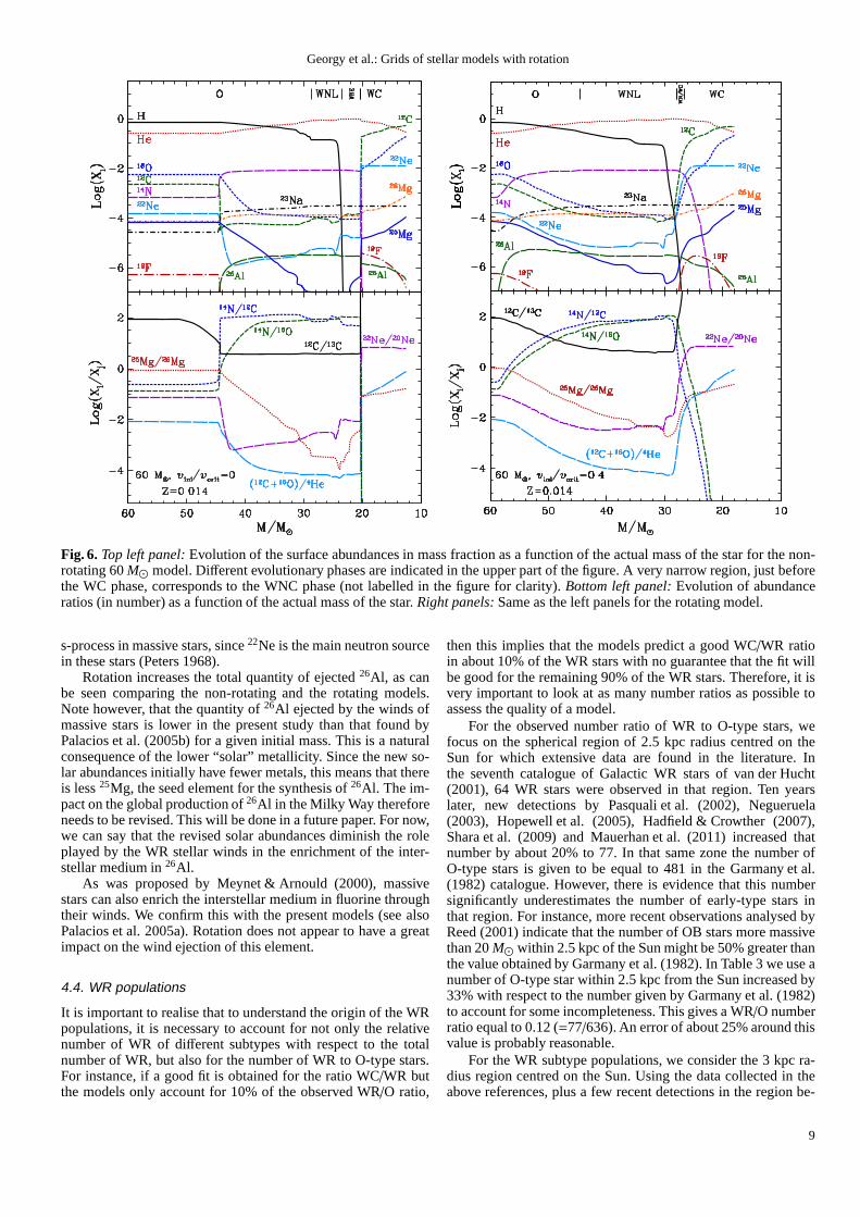
The O-type, WNL, WNE, WC, and WO phases are exclusive.The WNC phase lies between the WNE and WC phases. Wepoint out here that the observational classification of WR stars isbased on spectroscopic characteristics and not on surface abun-dances. A firm classification of our models would therefore re-quire computing the output spectrum. While some attempts inthat direction have already been made (Schaerer et al. 1996a,b;Schaerer & de Koter 1997), this is by far not yet a standard pro-cedure. We decided here to follow the usual procedure mostoften found in the literature to connect WR spectral types tosurface abundances. Below we present some numerical exam-ples that illustrate how numbers change when different rules areadopted for the connection between surface abundances and WRsubtypes. In Fig. 1 we show where each WR phase occurs in theHRD for the models between 20 and 120M⊙.

Comparing the rotating and non-rotating models, we note thefollowing differences:

– The MS rotating tracks for the most massive stars (M ≥

60M⊙ andvini ≥ 350 km s−1) follow a nearly homogeneousevolution during the MS phase (Maeder 1987). As a numeri-cal example, the mass fraction of hydrogen at the stellar sur-face is 0.32 in the rotating 120M⊙ model when the massfraction of hydrogen at the centre is 0.28. We note that al-though these models remain quite compact and hence blueduring the MS, their surface velocity decreases a lot. Indeed,at the end of the core H-burning phase, the surface velocityis only a few km s−1 for stars with initial masses equal or su-perior to 60M⊙. This is caused by the high mass-loss ratesundergone by these stars.

– Without rotation, only the 120M⊙ enters the WR phase atthe end of the MS, while with rotation, the 60M⊙ and moremassive stars already enter into the WR phase during the MSphase.

2 The duration of the corresponding WR phase is not very sensitive tothe choice of this limit if it remains in the range 0.3 – 0.4 as mentionedby Meynet & Maeder (2003).

– A small range of initial masses go through an RSGstage before entering the WR regime. These models reachlog(Teff/K) ∼ 3.5 at the RSG stage, and then, due to thestrong mass loss, evolve back to the blue part of the HRD.They finally become WR stars at the very end of their evolu-tion, ending as a WNL or WNE stars with an effective tem-perature (at the border of the hydrostatic core) of roughlylog(Teff/K) ∼ 4.5. Rotation restricts the mass domain of thefamily of tracks evolving into a WR phase after a RSG phase(see Fig. 2). As a consequence, rotation decreases the max-imum luminosity of the RSGs from 5.7 without rotation toabout 5.4 with rotation. The last value agrees better with theupper limit of RSGs, which was found by Levesque et al.(2005) to be between 5.2 and 5.4.

– The minimum luminosity reached by the WN and WC starsis given by the minimum initial masses of the stars that gothrough WNL and WC phases (see Table 2). They are low-ered by rotation: for non-rotating models, the minimum lu-minosity of WNL and WC stars is 5.37 and 5.5, respectively,while for the rotating models it is equal to 5.25 and 5.35, re-spectively,i.e. in the same range as the maximum luminosityfor RSG stars.

– Both rotating and non-rotating models predict that the leastluminous WR stars are WNL stars. The least luminous starsare produced by the least massive star that just succeeds toenter the WNL phase at the end of its evolution. Note that ifthe mass-loss rates are allowed to be higher than accountedfor in the present grid, there might be situations where theleast luminous stars would be WC stars originating fromstars well above the minimum initial mass of stars evolv-ing into a WR stage. This is what was obtained in the gridwith enhanced mass loss by Maeder & Meynet (1994), forinstance. The nature of the less luminous WR stars thereforedepends quite closely on the mass-loss rate history.

3.2. WR lifetimes and mass limits

The WR lifetimes are indicated in Table 1 and are plotted asa function of the initial mass in Fig. 2. The minimum massesleading to a WR star (or a subtype)MWR

min are given in Table 2.The mass limits are determined as in Georgy et al. (2009).

Qualitatively, the results do not differ from those presentedin previous papers (Meynet & Maeder 2003, 2005). The generaltrend is an increase of the WR phase lifetime with increasingmass and rotation. The most spectacular increase concerns theduration of the WNL phase for rotating models, which is severaltimes longer than for non-rotating ones. On the other hand, theWNE phase almost disappears for rotating models. Again, thisis a consequence of rotational mixing. To understand this, wehave to keep in mind a few specific points. First, a WNE phaseimplies some pure He layers, which obviously appear only whenH-burning is terminated in those layers. Second, the width inmass of the pure He-rich region, which when uncovered givesthe WNE phase, is decreasing rapidly with time because of thefast growing He-burning core that enriches the central layers incarbon and oxygen. Third, mixing prolongs the WNL stage, asjust seen above, and consequently leaves more time for the starto evolve into the core He-burning phase, which in turn reducesthe mass of pure He-layers. This makes the WNE phase veryshort in rotating models, or even more generally in any modelswith some efficient internal mixing.

3


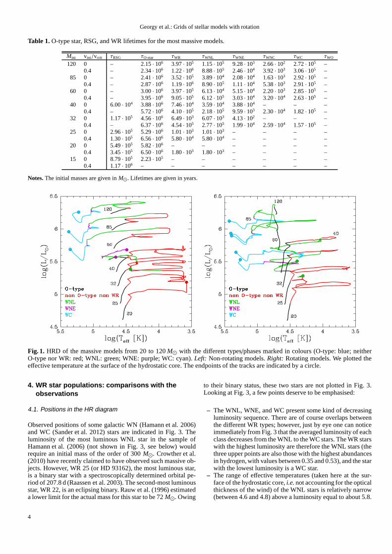
Table 1.O-type star, RSG, and WR lifetimes for the most massive models.

Mini vini/vcrit τRSG τO-star τWR τWNL τWNE τWNC τWC τWO

120 0 – 2.15 · 106 3.97 · 105 1.15 · 105 9.28 · 103 2.66 · 102 2.72 · 105 –0.4 – 2.34 · 106 1.22 · 106 8.88 · 105 2.46 · 104 3.92 · 103 3.06 · 105 –

85 0 – 2.41 · 106 3.52 · 105 3.89 · 104 2.08 · 104 1.63 · 103 2.92 · 105 –0.4 – 2.87 · 106 1.19 · 106 8.90 · 105 1.11 · 104 5.38 · 103 2.91 · 105 –

60 0 – 3.00 · 106 3.97 · 105 6.13 · 104 5.15 · 104 2.20 · 103 2.85 · 105 –0.4 – 3.95 · 106 9.05 · 105 6.12 · 105 3.03 · 104 3.20 · 104 2.63 · 105 –

40 0 6.00 · 104 3.88 · 106 7.46 · 104 3.59 · 104 3.88 · 104 – – –0.4 – 5.72 · 106 4.10 · 105 2.18 · 105 9.59 · 103 2.30 · 104 1.82 · 105 –

32 0 1.17 · 105 4.56 · 106 6.49 · 103 6.07 · 103 4.13 · 102 – – –0.4 – 6.37 · 106 4.54 · 105 2.77 · 105 1.99 · 104 2.59 · 104 1.57 · 105 –

25 0 2.96 · 105 5.29 · 106 1.01 · 103 1.01 · 103 – – – –0.4 1.30 · 105 6.56 · 106 5.80 · 104 5.80 · 104 – – – –

20 0 5.49 · 105 5.82 · 106 – – – – – –0.4 3.45 · 105 6.50 · 106 1.80 · 103 1.80 · 103 – – – –

15 0 8.79 · 105 2.23 · 105 – – – – – –0.4 1.17 · 106 – – – – – – –

Notes.The initial masses are given inM⊙. Lifetimes are given in years.

Fig. 1. HRD of the massive models from 20 to 120M⊙ with the different types/phases marked in colours (O-type: blue; neitherO-type nor WR: red; WNL: green; WNE: purple; WC: cyan).Left: Non-rotating models.Right: Rotating models. We plotted theeffective temperature at the surface of the hydrostatic core. The endpoints of the tracks are indicated by a circle.

4. WR star populations: comparisons with theobservations

4.1. Positions in the HR diagram

Observed positions of some galactic WN (Hamann et al. 2006)and WC (Sander et al. 2012) stars are indicated in Fig. 3. Theluminosity of the most luminous WNL star in the sample ofHamann et al. (2006) (not shown in Fig. 3, see below) wouldrequire an initial mass of the order of 300M⊙. Crowther et al.(2010) have recently claimed to have observed such massive ob-jects. However, WR 25 (or HD 93162), the most luminous star,is a binary star with a spectroscopically determined orbital pe-riod of 207.8 d (Raassen et al. 2003). The second-most luminousstar, WR 22, is an eclipsing binary. Rauw et al. (1996) estimateda lower limit for the actual mass for this star to be 72M⊙. Owing

to their binary status, these two stars are not plotted in Fig. 3.Looking at Fig. 3, a few points deserve to be emphasised:

– The WNL, WNE, and WC present some kind of decreasingluminosity sequence. There are of course overlaps betweenthe different WR types; however, just by eye one can noticeimmediately from Fig. 3 that the averaged luminosity of eachclass decreases from the WNL to the WC stars. The WR starswith the highest luminosity are therefore the WNL stars (thethree upper points are also those with the highest abundancesin hydrogen, with values between 0.35 and 0.53), and the starwith the lowest luminosity is a WC star.

– The range of effective temperatures (taken here at the sur-face of the hydrostatic core,i.e. not accounting for the opticalthickness of the wind) of the WNL stars is relatively narrow(between 4.6 and 4.8) above a luminosity equal to about 5.8.

4


Fig. 2.Lifetimes in the RSG phase (defined as stars with log(Teff/K) < 3.66, see Eldridge et al. 2008) and in the different phases ofWR stars.Left: Non-rotating models.Right: Rotating models.

Below, it widens and extends from 4.6 up to slightly morethan 5.

– The ranges of effective temperatures covered by the WNEand WC are similar and extend towards higher temperaturesthan the range of WNL stars. The difference in temperatureranges between the H-rich and the H-poor stars reflects thestrong dependency of the opacity on the quantity of hydro-gen.

Before comparing with the present evolutionary tracks, letus try to explain the features listed above in a general theoret-ical framework. We focus here on the luminosity and excludethe question of the effective temperature. The reason for that isthat the effective temperature depends a lot on the mass-loss rateused and on the physics of the outer layers, while luminosityisquite tightly related to the total mass of the star and its inter-nal physics. In that respect, it is a more fundamental quantity tocompare with models for the interior of stars.

The decrease in luminosity when passing from the WNL tothe WC stars might be interpreted in two ways. To obtain a WCstar from a given initial mass star, the star must lose more massthan what is required to obtain a WNL star, implying that onaverage WC stars have lower actual masses and consequentlyalso lower luminosities. Another way to interpret this feature(although not incompatible with the previous one) would be toassume that the most massive stars produce the high-luminosityWNL stars (which will then evolve into lower-luminosity WNEand WC-type stars), while the less massive stars produce theWCstars. In the framework of the single-star scenario, this last ex-planation requires very strong mass loss during the RSG phaseof stars with initial masses of about 15M⊙. This strong massloss could be caused by some physical processes originatinginthe envelope of the RSGs, while in the binary channel it couldbe caused by a RLOF process occurring in a close-binary sys-tem. Whatever process is invoked, it should not produce any longWNL or WNE phases at this low luminosity range since thesestars are not observed. This point will be discussed in more de-tail in Sect. 5.

Comparing the above observed positions with our rotatingstellar models we note the following features. The group ofseven very luminous stars (log(L/L⊙) ≥ 6.25) all show a massfraction of hydrogen higher than 10%, except in one case wherethe mass fraction is estimated to be 0.05 (see Fig. 4). In addition,no WNE and WC are observed in the luminosity range coveredby these stars. Is there any explanation for these two features?The reason why only H-rich WN stars are observed in this high-luminosity range supports the idea that WR stars form througha combination of mass-loss and radiative-zone mixing, and notonly through mass loss as in the non-rotating models. To illus-trate this, we have plotted in Fig. 5 the evolution as a function oftime of the mass fraction of hydrogen at the surface of our 60,85, and 120M⊙ stellar models with and without rotation duringthe WNL phase. We see that only the most massive star mod-els with rotation (M ≥ 60M⊙) present an H-rich surface duringsufficiently long periods (a few 100 thousands years) for allow-ing this phase to be observable. Corresponding models withoutrotation, or lower initial mass models, which enter into theWRphase only after the end of the MS phase, do not show any long“H-rich” periods and thus cannot account for the most luminousH-rich WNL stars. The absence of WNE and WC stars in this lu-minosity range may be explained by the fact, already mentionedabove, that WNE and WC stars are expected to be less massiveand therefore less luminous than WNL stars because more masshas to be removed from the star to reach those stages and/or be-cause they are produced from stars with lower initial masses.

Figure 4 shows the evolution of the mass fraction of hydro-gen at the surface as a function of the luminosity. Comparedto non-rotating models, the rotating ones extend the regionscovered by the WNL and WNE stars to a lower luminosity.However, the change remains modest so that comparisons withobservations hardly allow one set to be favoured over the other.As emphasised above, the time spent in the H-rich portion of thediagram is probably much more decisive and favours the rotatingmodels. We see that the tracks cover the region where the WNLstars are observed. The extension in luminosity of the WNE stars

5


Table 2.Mass ranges for the various WR- and SN-remnant-types (inM⊙) deduced from our models, and comparison with previousworks.

O-type WNL WNE WCThis work

rot. 15.8 – 20.0 20.0 – 25.3 25.3 – 27.0 27.0 – 120.0no rot. 15.0 – 25.0 25.0 – 31.7 31.7 – 40.5 40.5 – 120.0

This work (High WNE1 )rot. 15.8 – 20.0 20.0 – 21.6 21.6 – 27.0 27.0 – 120.0

no rot. 15.0 – 25.0 25.0 – 29.2 29.2 – 40.5 40.5 – 120.0Georgy et al. (2009)

rot. 23.0 – 26.0 26.0 – 29.0 29.0 – 120.0SN II-P SN II-L/n SN Ib SN Ic

BH→

brig

htS

N3

This work (low SN Ic2 )rot. 8.0 – 16.8 16.8 – 25.0 25.0 – 31.1 31.1 – 39.1

39.1 – 120.0no rot. 8.0 – 19.0 19.0 – 32.0 32.0 – 120.0

This work (medium SN Ic2 )rot. 8.0 – 16.8 16.8 – 25.0 25.0 – 30.1 30.1 – 82.0

82.0 – 88.7 88.7 – 120.0no rot. 8.0 – 19.0 19.0 – 32.0 32.0 – 52.2 52.2 – 106.4

106.4 – 120.0This work (high SN Ic2 )

rot. 8.0 – 16.8 16.8 – 25.0 25.0 – 29.0 29.0 – 120.0no rot. 8.0 – 19.0 19.0 – 32.0 32.0 – 44.8 44.8 – 120.0

BH→

nobr

ight

SN4

This workno rot. 8.0 – 19.0 19.0 – 32.0 32.0 – 43.8

This work (low SN Ic2 )rot. 8.0 – 16.8 16.8 – 25.0 25.0 – 31.1 31.1 – 33.9

This work (medium SN Ic2 )rot. 8.0 – 16.8 16.8 – 25.0 25.0 – 30.1 30.1 – 33.9

This work (high SN Ic2 )rot. 8.0 – 16.8 16.8 – 25.0 25.0 – 29.0 29.0 – 33.9

Georgy et al. (2009)rot. 8.0 – 25.0 25.0 – 39.0 39.0 – 120.0

Notes.All masses are given inM⊙.(1) Considering that the surface He abundance limit between WNLand WNE is 0.1 instead of 10−5.(2) The maximum He mass ejected allowed to be still considered asa Type Ic SN is 0.4 - 0.6 - 0.8M⊙ in the low - medium - high SN Ic caserespectively (see Georgy et al. 2009).(3) Assuming that the formation of a BH during the collapse has noinfluence on the SN explosion.(4) Assuming that the formation of a BH during the collapse prevents a bright SN explosion.

is also well reproduced, somewhat supporting the present single-star models for explaining these populations.

A serious difficulty is the low observed luminosity of someWC stars. Our present tracks predict a lower luminosity limit forthe WC stars of 5.35 (in log(L/L⊙)), while the lowest luminosityplotted in Fig. 3 is about 4.9 according to the revised spectralanalyses of galactic WC stars by Sander et al. (2012). We discussthis point in more detail below.

4.2. Discussion of various possible origins for thelow-luminosity WC stars

What might be the origin of the observed low-luminosity (andthus low-mass) WC stars? If the luminosity is not underesti-mated at present, we can imagine three different kinds of evo-lutionary scenarios:

1. Stars with initial masses between 15 and 20M⊙ lose muchmore mass than in the present grid of models during theirRSG stage. We shall refer to this scenario as theRSG sce-nario.

2. Stars with initial masses above about 25M⊙ lose much moremass than in the present grid of models (the massive starscenario).

3. The low-mass WC stars are produced in close-binary sys-tems through RLOF. This process can indeed produce lowerfinal masses, as illustrated, for instance, by the recent mod-els of Yoon et al. (2010). We shall refer to this scenario astheclose-binary (CB) scenario.

Let us now discuss the advantages and disadvantages of each ofthese three scenarios.

1. The RSG scenario. There are some mass-loss rate de-terminations for RSG pointing towards very high values. Forinstance, van Loon et al. (2005) obtained that dust-enshroudedRSGs present mass-loss rates that are a factor of 3–50 timeshigher than the rate of de Jager et al. (1988). Humphreys et al.(1997, 2005) and Smith et al. (2009) also indicated that the RSGstar VY CMa went through important episodic mass ejections500–1000 years ago. Moriya et al. (2011) reached similar con-clusions, studying the luminosity curve of SNe with RSG pro-genitors. Their results indicate that some mechanism is proba-bly inducing extensive mass loss (greater than 10−4 M⊙ yr−1) inmassive RSGs just before their explosions. Humphreys (2008)

6


Fig. 3. Positions of observed WN and WC stars in the HRD asgiven by Hamann et al. (2006) and Sander et al. (2012), respec-tively. The empty circles are WNL stars, and the full trianglesare WNE. The WC stars are represented by pentagons, filledwhen the distance is known and empty when it is unknown. Thepresent rotating tracks are superposed.

Fig. 4. Evolution of the mass fraction of hydrogen at the sur-face as a function of the luminosity. The continuous lines arethe present rotating models, while the dotted lines represent thenon-rotating ones. The dots are the WN stars with non-zeroH-abundance and the shaded zone shows the range in lumi-nosity of the WN stars with no H detected at the surface byHamann et al. (2006). The triangles are LBV stars (Groh et al.2009; Lamers et al. 2001). In this graph, models start at the topon the MS. They evolve to the right as their luminosity increasesand downwards with mass loss peeling off the hydrogen-rich lay-ers. The most massive models evolve back to the left (decreasingluminosity) due to the strong mass loss in the WR phase.

Fig. 5.Evolution of the mass fraction of hydrogen at the surfaceas a function of time during the WNL phase. The continuous redlines correspond to rotating models, while the dashed blacklinescorrespond to non-rotating ones. The corresponding massesareindicated near the curves.

suggests that convective/magnetic activity may be the cause forwhat does appear as episodic and localised mass-loss events.Also very interesting are the observations by Davies et al. (2008)of the so-called RSG clusters in the direction of Scutum. Maseremission indicative of a high-density medium above the photo-sphere is observed around the most luminous RSGs. This can becaused by the high mass-loss rates experienced by these stars.The presence of a luminous yellow supergiant in one of theseclusters is also consistent with the idea that this star evolvedaway from the RSG stage (Davies et al. 2008).

Mauron & Josselin (2011), on the other hand, still recom-mend using the de Jager et al. (1988) rate for Galactic RSGs,indicating that this prescription agrees to within a factorof 4with most mass-loss rate estimates based on the infrared 60µmexcess. This result is however compatible with the existence ofshort phases during which the mass-loss rates are much stronger.Indeed, mass-loss rates during the RSG phase may present someoutbursting characteristics, somewhat similar (at lower luminos-ity and effective temperature) to what happens at higher lumi-nosity and effective temperature for the luminous blue variable(LBV) stars (Smith et al. 2011). The physical reasons for thesehigh mass-loss rates may be related to the pulsational proper-ties of RSGs (Yoon & Cantiello 2010) and/or to the appearanceof super-Eddington luminosities in the outer layers of the star(Paper I).

From the theoretical point of view, it is well known thatstrong mass loss during the RSG phase favours a bluewards evo-lution (Salasnich et al. 1999; Vanbeveren et al. 1998, 2007)andthus helps in fulfilling one of the two minimal conditions forhav-ing a WR star, namely to have an effective temperature higherthan about log(Teff/K) = 4.0. However, it is unclear whether thisstrong mass loss may lead to the formation of WC stars. Georgy(2012) has shown that increased mass-loss rates during the RSGphase (up to a factor of 10) are insufficient to lead to a WR starat the end of the evolution. To be valid, the RSG scenario should

7


therefore involve a very strong increase of the mass-loss rate ofmore than 10 times during that phase with respect to the standardone.

One can already note that it will be difficult to separate thephysical reason for the envelope loss, determining whetherit iscaused by a physical process occurring in the envelope of thestar(as would be the case in the single-star channel) or to a RLOF.Aconstraint on this scenario may come from the fact that therearevery few (if any) single-age clusters that simultaneously showRSGs and WR stars (Humphreys et al. 1985), except in the clus-ters at the centre of our Galaxy (Figer 2007) and in Westerlund1 (Negueruela et al. 2010, although in the latter case we may seetwo clusters aligned instead of only one, as in the case of theDansk clusters; see Davies et al. 2012). If some WR stars areproduced from a range of initial masses that are also producingRSG, then to be consistent with this observation, either theRSGduration or the WR duration should be very short.

2. The massive star scenario. In the high mass-loss rate gridof Meynet et al. (1994), a very low luminosity is reached forWC stars due to heavy mass loss. The lowest luminosity forthe WC stars was at 4.5 and originated from the evolution of a120M⊙! The high mass-loss rates used in Meynet et al. (1994)are no longer supported by the more recent mass-loss determi-nations for O-type and WR stars that account for the effects ofclumping (Vink et al. 2001; Nugis & Lamers 2000). However,very massive stars could lose very large amounts of mass invery short periods during which a strong mass outburst occurs(Smith & Owocki 2006). Therefore, it is possible that the mass-loss determination, necessarily based on more frequent “normal-moderate” mass-loss rate stages, actually underestimatesthe truetime-averaged mass-loss rate.

3. The CB scenario. In close binaries, the primary can loseits H-rich envelope during RLOF phases. The secondary can alsoundergo such a loss. The two stars may also merge or enter intoa common-envelope phase leading to heavy mass loss episodes.Clearly, these evolutionary scenarios can lead to the produc-tion of WR stars and therefore have an impact on their pop-ulations. For instance, the close-binary scenario of Yoon et al.(2010) makes it possible to produce final masses in the range be-tween 1 and 7M⊙, even when starting from high initial masses(as for instance a 60M⊙, see Yoon et al. 2010). However, ac-cording to the review by Crowther (2007, see Fig. 4), the leastmassive WC star whose mass has been determined from binaryorbit has a mass of about 9M⊙ (the most massive has about16M⊙). The recent analysis of Galactic WC stars performed bySander et al. (2012) gives masses between 8 and 37M⊙, cov-ering quite well the masses obtained by our single-star models(10 – 26M⊙). Therefore, the least massive He-core produced bythe close-binary scenario cannot be invoked to explain the low-luminosity WC stars.

Close-binary evolution can produce WR stars from lowerinitial masses than the single-star evolutionary channel.For in-stance, Eldridge et al. (2008) found that the minimum initialmasses for stars to become WC stars is lowered from about27M⊙ in the single-star scenario to 15M⊙ in the close-binaryscenario. In the mass range between 15 and 25M⊙, the WCstage occurs only at the very end of the evolution and has a du-ration of the order of 104 years. This supports the view that low-luminosity WC stars could indeed be the result of close-binaryevolution. It remains to be seen whether this scenario is able toexplain the observed number of low-luminosity WC stars as wellas their masses.

Accordingly at the moment, the three scenarios describedabove may contribute in explaining the low-luminosity WC

stars. To investigate the relative weight of these different scenar-ios, progress must be made in several directions. We need to con-strain the occurrence of short and strong mass-ejection episodesduring the RSG phase. Could these events allow stars with initialmasses around 15M⊙ to evolve into a WR phase?

Is there any evidence that the low-luminosity WC stars areproduced in close-binary systems? Positive evidence couldin-clude the presence of a companion, or the determination thatthese stars are runaway stars, kicked off when the primary ex-ploded in an SN event. Note however, that runaway stars mayalso be produced by dynamical interactions in dense clusters andthus result from processes other than binarity.

Is there any evidence for the presence of low-luminosityWC stars in very young associations, typically with a mass atthe turnoff above about 25M⊙? These low-luminosity WC starswould originate from an initial mass more massive than 25M⊙and this would support the second scenario (the massive starsce-nario).

4.3. Surface chemical compositions

In Fig. 6, the evolution of the surface abundances is shownfor the non-rotating and rotating 60M⊙ models. As alreadynoted by Meynet & Maeder (2003) (see also Maeder 1987;Fliegner & Langer 1995), one of the main effects of rotation is tosmooth the internal chemical gradients and to favour a more pro-gressive arrival of internal nuclear products at the surface. Thisis well apparent comparing the curves shown in the left and rightpanels of Fig. 6.

One observable consequence is that rotating models predictmore extended phases during which both H- and He-burningproducts are seen at the surface (Langer 1991). Note that in theleft panel of Fig. 6, the WNC phase is so narrow that it only ap-pears as a thicker tick in the upper part of the top panel, while inthe right panel of Fig. 6, a well-extended phase is present. Thisphase overlaps with the WNE phase, which is not shown in thefigure for clarity.

Except for this effect, rotation leaves no other easily observ-able imprints on the way the surface composition evolves. Thisis quite expected because CNO equilibrium values are obtainedduring the WN phase that can be deduced from the nuclear prop-erties of the chemical species and are not strongly affected by thedetails of the considered stellar model.

This is also true for the abundance of22Ne obtained duringthe WC phase. The abundance of22Ne at this stage (WC) is actu-ally an indication of the initial CNO content of the star. Indeed,22Ne comes mainly from the destruction of14N at the beginningof the helium-burning phase. This14N is the result of the trans-formation of carbon and oxygen into nitrogen operated by theCNO cycle during the core H-burning phase.

It is interesting to note that comparing the observed Ne/Heratios at the surface of WC stars with models computed withZ = 0.020 shows that models over-predict the Ne abun-dance, while models starting with the solar abundances givenby Asplund et al. (2005) yield a much better fit, as can be seenin Fig. 7. This confirms that massive stars in the solar neighbour-hood have initial metallicities that agree with the Asplundet al.(2005) solar abundances.

Let us note that this overabundance of22Ne at the surface ofWC stars is not only an important confirmation of the nuclearreaction chains occurring during He-burning, but is also relatedto the questions of the origin of the material accelerated intogalactic cosmic rays (Binns et al. 2005) and to that of the weak

8


Fig. 6. Top left panel: Evolution of the surface abundances in mass fraction as a function of the actual mass of the star for the non-rotating 60M⊙ model. Different evolutionary phases are indicated in the upper part ofthe figure. A very narrow region, just beforethe WC phase, corresponds to the WNC phase (not labelled in the figure for clarity).Bottom left panel: Evolution of abundanceratios (in number) as a function of the actual mass of the star. Right panels: Same as the left panels for the rotating model.

s-process in massive stars, since22Ne is the main neutron sourcein these stars (Peters 1968).

Rotation increases the total quantity of ejected26Al, as canbe seen comparing the non-rotating and the rotating models.Note however, that the quantity of26Al ejected by the winds ofmassive stars is lower in the present study than that found byPalacios et al. (2005b) for a given initial mass. This is a naturalconsequence of the lower “solar” metallicity. Since the newso-lar abundances initially have fewer metals, this means thatthereis less25Mg, the seed element for the synthesis of26Al. The im-pact on the global production of26Al in the Milky Way thereforeneeds to be revised. This will be done in a future paper. For now,we can say that the revised solar abundances diminish the roleplayed by the WR stellar winds in the enrichment of the inter-stellar medium in26Al.

As was proposed by Meynet & Arnould (2000), massivestars can also enrich the interstellar medium in fluorine throughtheir winds. We confirm this with the present models (see alsoPalacios et al. 2005a). Rotation does not appear to have a greatimpact on the wind ejection of this element.

4.4. WR populations

It is important to realise that to understand the origin of the WRpopulations, it is necessary to account for not only the relativenumber of WR of different subtypes with respect to the totalnumber of WR, but also for the number of WR to O-type stars.For instance, if a good fit is obtained for the ratio WC/WR butthe models only account for 10% of the observed WR/O ratio,

then this implies that the models predict a good WC/WR ratioin about 10% of the WR stars with no guarantee that the fit willbe good for the remaining 90% of the WR stars. Therefore, it isvery important to look at as many number ratios as possible toassess the quality of a model.

For the observed number ratio of WR to O-type stars, wefocus on the spherical region of 2.5 kpc radius centred on theSun for which extensive data are found in the literature. Inthe seventh catalogue of Galactic WR stars of van der Hucht(2001), 64 WR stars were observed in that region. Ten yearslater, new detections by Pasquali et al. (2002), Negueruela(2003), Hopewell et al. (2005), Hadfield & Crowther (2007),Shara et al. (2009) and Mauerhan et al. (2011) increased thatnumber by about 20% to 77. In that same zone the number ofO-type stars is given to be equal to 481 in the Garmany et al.(1982) catalogue. However, there is evidence that this numbersignificantly underestimates the number of early-type stars inthat region. For instance, more recent observations analysed byReed (2001) indicate that the number of OB stars more massivethan 20M⊙ within 2.5 kpc of the Sun might be 50% greater thanthe value obtained by Garmany et al. (1982). In Table 3 we use anumber of O-type star within 2.5 kpc from the Sun increased by33% with respect to the number given by Garmany et al. (1982)to account for some incompleteness. This gives a WR/O numberratio equal to 0.12 (=77/636). An error of about 25% around thisvalue is probably reasonable.

For the WR subtype populations, we consider the 3 kpc ra-dius region centred on the Sun. Using the data collected in theabove references, plus a few recent detections in the regionbe-

9


Fig. 7. Variations of the abundance ratios Ne/He vs. C/He at thesurface of WC stars (in number). Models are represented by thelines (the Z=0.014 are the rotating models of the present paper,theZ = 0.020 is the rotating model of Meynet & Maeder 2003).The points are the observed values by Dessart et al. (2000) (filledcircles) and Crowther (2006).

tween 2.5 and 3 kpc (Mauerhan et al. 2009; Roman-Lopes 2011;Anderson et al. 2011), there are 45 WN and 55 WC stars as dif-ferent subtypes of WR stars. The 45 WN stars are distributedbetween 21 WNL, 23 WNE and 1 WNC stars. It must be em-phasised here that the respective portion of WNL and WNE starsis quite uncertain. Where information on the mass fraction of Hwas available, we used the presence of H to classify a star as aWNL star and the non-detection of hydrogen for classifying it asa WNE star. For this we used the sample of Galactic WN starsanalysed by Hamann et al. (2006), which has 20 stars in com-mon with our sample of nearby WR stars. We classified in theremaining 25 stars all stars with an “h”, indicative of the pres-ence of hydrogen, as WNL, as well as all stars with spectral typeequal or later than WN7; the remaining stars are considered tobe WNE stars. Again, assuming an error of about 25% we obtainthe range of values given in Table 3. The WNC star is special inthe sense that there is only one star of this type in the solar neigh-bourhood, which represents 1% of WR stars in that same region.Among the WR stars presently detected in the Galaxy (476 ac-cording to Mauerhan et al. 2011, but 548 if we add the 72 newWR detections by Shara et al. 2011), 9 are at present identifiedas WNC stars, which corresponds to a proportion of about 2%.Therefore we indicate a range between 1 and 2% for this ratio inTable 3.

To compute the ratio of two types of stellar populations (Aand B), we have to know the initial mass range leading to eachpopulation

[

MAmin ...M

Amax

]

and[

MBmin ...M

Bmax

]

, as well as the

time spent in the corresponding phaseτA andτB. When a con-stant star formation rate is assumed, the ratio of the two popula-tions is given by

N(A)N(B)

=

∫ MAmax

MAminφ(M)τA(M)dM

∫ MBmax

MBminφ(M)τB(M)dM

, (1)

whereφ(M) is the initial mass function. Here we consider aSalpeter initial mass function (IMF) (Salpeter 1955). The resultsare presented in Table 3.

The predicted value for the rotating models corresponds toonly one initial vini/vcrit value (0.4). A detailed computationshould account for a distribution of the initial velocities. Sincethe value of 0.4 has been chosen to reproduce the average ob-served surface velocities during the MS for B stars (Huang etal.2010), we expect that the values of the ratios obtained for thisparticular value are close to the value that would be obtained bya properly weighted averaging over an initial velocity distribu-tion (assuming that the characteristic initial ratiovini/vcrit is thesame for more massive stars).

The value of the WR/O ratio given by the non-rotatingsingle-star model is 0.02, which is quite low compared to theobserved ratio of around 0.12. The low ratio results from thelow mass-loss rates used here that account for the clumping ef-fect. If these models were the correct ones, then it would meanthat close-binary evolution is responsible for more than 80% ofthe WR stars. However, since rotating models better fit manyobserved features of massive stars (such as, for example, thechange of the surface abundances), their predictions are tobepreferred to those obtained from the non-rotating models. TheWR/O value obtained by the rotating models, 0.07, is more thanthree times the value obtained by the non-rotating models. It isbelow the observed values, which leaves some room for∼ 40%of binaries from the close-binary scenario to contribute tothenumber of WR stars at solar metallicity.

Since the WNL phase is increased in duration by rotation, theWNL/WR ratio is increased when the rotating models are used.The WNE/WR and WC/WR ratios, in contrast, decrease. Thefew WNC stars can be very well explained by internal mixingprocesses.

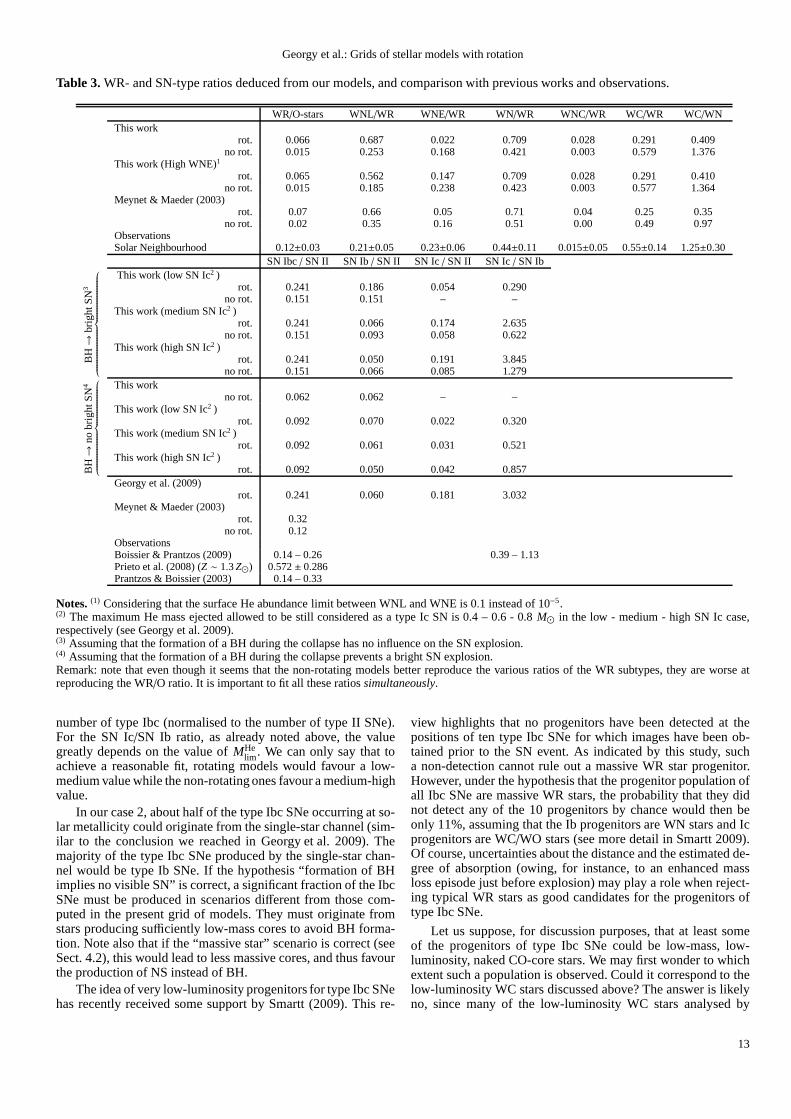
To confront the present theoretical predictions with theobserved numbers, we followed the same formalism as inMaeder & Meynet (1994). WRs is the number of WR stars thatdo not require any mass transfer episode for entering into theirWR phase, and WRcb are those WR stars that owe their WR na-ture to a previous RLOF mass transfer. The total ratio WR/O canbe written as the sum WRs/O+WRcb/O.ϕ is the ratio WRcb/O.Below we consider that the WNC stars are produced by internalmixing only, not by a binary mass-transfer event. In principle, aWNC star might result from a WN star that accretes matter froma WC star, but this does not appear to be realistic for at leasttworeasons: first, because of the compactness of these types of stars,some very peculiar initial conditions for the mass ratio andtheperiod of the orbit are likely necessary; second, both typesofstars suffer strong stellar winds, and processes such as wind col-lisions are more likely to occur than accretion. The WNC/WRratio will therefore depend onϕ only through the dependence ofthe total number of WR.

The first three upper panels of Fig. 8 show how the WR/O,WNC/WR and WRcb/WR3 compare to observations for differentvalues ofϕ, using the results of the present rotating models forthe fractions obtained whenϕ = 0. We see that the range ofvalues forϕ compatible with the observations is between 0.03and 0.075, which corresponds to situations when 31 to 53% ofthe WR stars owe their WR nature to a RLOF episode.

To further pursue this line of reasoning and use comparisonswith the observed WNL, WNE and WC star number ratios, weneed to make some assumptions about the distributions in the

3 The fraction of WR due to close-binary evolution with respect tothe total number of WR stars is given byϕ/(WRs/O+ ϕ).

10


Fig. 8. Variations of various number ratios as a function ofϕ = WRcb/O, the fraction of WR stars with respect to O-typestars that owe their nature as WR stars to a RLOF episode in aclose-binary system. The continuous lines in the 4 lower panelsare the models forϕWNL , ϕWNE, ϕWNC andϕWC equal to 0, 0,0.3ϕ, and 0.7ϕ respectively (see text). The horizontal strips cor-respond to observed ratios as reported in Table 3. The green partcorresponds to the values ofϕ allowed by the observation, andthe red one the excluded values.

WR subtypes resulting from the close-binary channel. We de-fine ϕWNL as WNLcb/WRcb. Analog definitions are consideredfor the other WR subtypes. With these definitions, the ratio ofWR(st)/WR where “st” designates a given subtype can be writ-ten

WR(st)WR

=

WRs(st)WRs

+ϕstϕ

WRs/O

1+ ϕ

WRs/O

. (2)

The values of the different components ofϕ should of course bethe outcome of close-binary evolution calculations, such as thoseperformed by Eldridge et al. (2008). Here, however, let us trya simpler approach guided by the comparisons of the observedratios with the predictions of the rotating models.

For the reasons laid out above, we assume thatϕWNC = 0.The WNL/WR ratio given by the present single-star rotatingmodels is well above the observed range. This ratio thereforeneeds to be reduced when the close-binary scenarios are ac-counted for. To go in that direction we make the extreme as-sumption thatϕWNL = 0. Even so, we see that a very high frac-tion of binaries would still be needed, which would be clearlyincompatible with the observed WR/O. This may indicate that

Fig. 9. Same as in Fig. 8, but considering that WNE stars areWN stars with less than 10% of hydrogen at the surface (massfraction).

the WNL phase is somewhat overestimated in the present mod-els4.

Considering thatϕWNE = 0.3ϕ andϕWC = 0.7ϕ, we find aconsistent solution forϕ = 0.075 for all ratios shown in Fig. 8,with the exception of the WNL/WR ratio, which is above theobserved range. At this point we conclude that mainly becauseof the high WNL/WR ratio obtained from the present models,we do not succeed in finding a completely consistent solution.To improve the situation, two lines of investigations can befol-lowed, one observational and one theoretical.

From the observational point of view, it is difficult to matchtheoretical criteria and observational ones. For example,howmuch H can be hidden in an observed WNE? Obtaining new reli-able measurements of the H abundance in all WN stars of the so-lar neighbourhood is crucial to find a better criterion for linkinga given structure obtained in stellar models to an observed WRsubtype. Some stars have changed classifications when more re-fined observations have been performed, indicating that thedis-tinction between WNL and WNE is not always clear-cut. To il-lustrate how the WNL/WR and WNE/WR fractions depend onthe definition of WNE, we indicate in Table 3 the ratios obtainedassuming that WNE stars are all WN stars with less than 10%of hydrogen at the surface (“high-WNE case”, see Tables 2 and3). We also show in Fig. 9 how the theoretical ratios compare

4 We recall that here we only consider one value ofvini/vcrit; thevalue obtained by a proper averaging over an initial velocity distribu-tion would likely be lower than that obtained from the uniquevalue ofvini/vcrit = 0.4

11


with the observations. When adopting this new definition fortheWNE stars, the WNE/WR ratio increases from 0.022 to 0.147,nearly a factor of 7. A consistent solution is now obtained for allratios and forϕ ∼ 0.07, which corresponds to a share of about50-50 between the single and binary channel for producing theobserved WR populations atZ = 0.014.

From the theoretical approach, one would explore a differentmass-loss rate history during the WNL and WNE phases. Forinstance, are the WN mass-loss rates the same when the star isacore H-burning star or a core He-burning one? Are the mass-lossrates during the WNE phase overestimated at present? Stellarmodels in the future may explore the consequences of differentprescriptions and offer some guidelines for improving the situa-tions.

5. Progenitors of type Ibc supernovae

The questions that we shall address in this section are the fol-lowing ones:

– What are the predictions of the present models for the fre-quency of type Ib and Ic SNe?

– How do these predictions compare to the observed ratios?– Can we find a consistent picture for understanding both the

WR populations as observed in the solar neighbourhood andthe frequency of type Ibc SNe, including contributions ofclose-binary evolution?

– Which fraction of the present models would produce afast rotating BH, accompanied by a type Ic SNe? The lastquestion is triggered by the possibility that stars showingthese conditions may give birth to a collapsar, proposed byWoosley (1993) as progenitors of LGRBs.

5.1. Predictions of the models

To determine the type of the SN that occurs at the end of theevolution of our massive star models, we used the same pro-cedure as in Georgy et al. (2009). We recall here a few mainpoints. First, we obtain the baryonic mass of the remnant us-ing the same relation between the CO-core mass and the rem-nant baryonic mass as in Maeder (1992). This mass is thenused to compute the gravitational mass of the remnant, withthe relation given in Hirschi et al. (2005). The results are givenin Table 4. Using these data, we estimate the maximal masson the zero-age main sequence (ZAMS) producing an NS dur-ing the SN event. As in Georgy et al. (2009), we consider themost massive NS to be 2.7 M⊙. This choice is somewhat sup-ported by the recent discovery of a very massive 2.4 M⊙ NS byvan Kerkwijk et al. (2011). We find thatMNS-BH

lim = 33.9 M⊙ (ro-tation), andMNS-BH

lim = 43.8 M⊙ (no rotation). The difference isexplained by the rotational mixing, which increases the size ofthe core. These limits are only poorly constrained, however, dueto uncertainties during the explosion process, which are not ac-counted for in our simple estimate (for example, the amount ofmatter that falls back, etc., see Fryer 2006).

Once the baryonic mass of the remnant is known, we deducethe composition of the ejecta, assuming that the entire massbe-tween the surface and the edge of the remnant is ejected duringthe SN event. The results are shown in Table 4. In the same table,we also indicate the SN type, using the chemical compositionof the ejecta and following the same criteria as in Georgy et al.(2009):

– If there is some hydrogen in the ejecta, the SN is a type II.

– If there is no hydrogen and a helium mass higher than a givenvalue (MHe

lim), it is a type Ib.– If there is no hydrogen and a helium mass lower thanMHe

lim ,it is a type Ic.

Accounting for the uncertainty ofMHelim , we give three values for

the mass limit between types Ib and Ic SNe, withMHelim = 0.4 M⊙

(low SN Ic, as this criterion favours type Ib SNe),MHelim = 0.6 M⊙

(medium case), andMHelim = 0.8 M⊙ (high SN Ic, as it favours

type Ic SNe).Recently, Dessart et al. (2011) found that some amount of

He can be unobservable in the spectrum of an SN when it is lo-cated primarily in the most external layers (up to 50% of He inmass fraction in the first 1M⊙ immediately below the surface).In this case, our non-rotating 120M⊙ and rotating 85M⊙ mod-els would be classified as a type Ic SN instead of type Ib. Thiscriterion thus produces the same mass limit between type Ib andtype Ic SNe as in the “high SN Ic” case (see Table 3).

Contrarily to Georgy et al. (2009), where no distinction wasconsidered between the various subtypes of type II SNe, we addin this work the same criterion as in Heger et al. (2003) to distin-guish between the type II-P SNe, and the type II-L or II-b SNe(owing to the weak statistics of these events, there is no simpleway to distinguish between type II-L and II-b on the basis of theejecta composition only. We therefore consider them as a uniquesample):

– A type II SN is considered to be a type II-P if the ejectacontains more than 2M⊙ of H.

– In the other case, it is considered to be a type II-L/b.

We see from Table 4 that the upper mass limit for type II-P SNwould be between 15 and 20M⊙ for both non-rotating and rotat-ing models. More precise mass limits can be obtained by inter-polation. The mass limits become 19.0 M⊙ for the non-rotatingmodels and 16.8 M⊙ for the rotating ones. Both values agreewith the results by Smartt et al. (2009).

We computed the various SN type ratios with the samemethod as in Georgy et al. (2009), with the same IMF. We con-sidered two cases: 1) a SN event is visible even when a BH isformed; 2) no visible SN occurs when a BH is formed. The re-sults are shown in Table 3. They are quite similar to those ob-tained with different models by Meynet & Maeder (2003, 2005),Georgy et al. (2009). Therefore, these results show some robust-ness against many changes in the physical ingredients of themodels.

We see that rotation increases the SN Ibc/SN II ratio by about60% (48%) in case 1 (2). The share of SN type Ibc between theIb and the Ic types depends on the value chosen forMHe

lim . Alow value implies more restrictive possibilities to obtaina SNIc and consequently a lower SN Ic/SN II ratio and a higher SNIb/SN II ratio. The trend of having more Ic SNe when rotation isaccounted for remains true for allMHe

lim considered here: rotationdecreases the minimum initial mass of stars finishing their lifeas WC (see Table 2). The effect of rotation on the SN Ib/SN IIratio is less clear: the ratio increases or decreases when rotationis accounted for depending onMHe

lim .

5.2. Comparisons with observations

At solar metallicity, in case 1, the present models give ratioswell within the range of the observed values determined byBoissier & Prantzos (2009). Indeed, one sees that the presentsingle-star models may explain the greatest part of the observed

12


Table 3.WR- and SN-type ratios deduced from our models, and comparison with previous works and observations.

WR/O-stars WNL/WR WNE/WR WN/WR WNC/WR WC/WR WC/WNThis work

rot. 0.066 0.687 0.022 0.709 0.028 0.291 0.409no rot. 0.015 0.253 0.168 0.421 0.003 0.579 1.376

This work (High WNE)1

rot. 0.065 0.562 0.147 0.709 0.028 0.291 0.410no rot. 0.015 0.185 0.238 0.423 0.003 0.577 1.364

Meynet & Maeder (2003)rot. 0.07 0.66 0.05 0.71 0.04 0.25 0.35

no rot. 0.02 0.35 0.16 0.51 0.00 0.49 0.97ObservationsSolar Neighbourhood 0.12±0.03 0.21±0.05 0.23±0.06 0.44±0.11 0.015±0.05 0.55±0.14 1.25±0.30

SN Ibc / SN II SN Ib / SN II SN Ic / SN II SN Ic / SN Ib

BH→

brig

htS

N3

This work (low SN Ic2 )rot. 0.241 0.186 0.054 0.290

no rot. 0.151 0.151 – –This work (medium SN Ic2 )

rot. 0.241 0.066 0.174 2.635no rot. 0.151 0.093 0.058 0.622

This work (high SN Ic2 )rot. 0.241 0.050 0.191 3.845

no rot. 0.151 0.066 0.085 1.279

BH→

nobr

ight

SN4

This workno rot. 0.062 0.062 – –

This work (low SN Ic2 )rot. 0.092 0.070 0.022 0.320

This work (medium SN Ic2 )rot. 0.092 0.061 0.031 0.521

This work (high SN Ic2 )rot. 0.092 0.050 0.042 0.857

Georgy et al. (2009)rot. 0.241 0.060 0.181 3.032

Meynet & Maeder (2003)rot. 0.32

no rot. 0.12ObservationsBoissier & Prantzos (2009) 0.14 – 0.26 0.39 – 1.13Prieto et al. (2008) (Z ∼ 1.3Z⊙) 0.572± 0.286Prantzos & Boissier (2003) 0.14 – 0.33

Notes.(1) Considering that the surface He abundance limit between WNLand WNE is 0.1 instead of 10−5.(2) The maximum He mass ejected allowed to be still considered asa type Ic SN is 0.4 – 0.6 - 0.8M⊙ in the low - medium - high SN Ic case,respectively (see Georgy et al. 2009).(3) Assuming that the formation of a BH during the collapse has noinfluence on the SN explosion.(4) Assuming that the formation of a BH during the collapse prevents a bright SN explosion.Remark: note that even though it seems that the non-rotatingmodels better reproduce the various ratios of the WR subtypes, they are worse atreproducing the WR/O ratio. It is important to fit all these ratiossimultaneously.

number of type Ibc (normalised to the number of type II SNe).For the SN Ic/SN Ib ratio, as already noted above, the valuegreatly depends on the value ofMHe

lim . We can only say that toachieve a reasonable fit, rotating models would favour a low-medium value while the non-rotating ones favour a medium-highvalue.

In our case 2, about half of the type Ibc SNe occurring at so-lar metallicity could originate from the single-star channel (sim-ilar to the conclusion we reached in Georgy et al. 2009). Themajority of the type Ibc SNe produced by the single-star chan-nel would be type Ib SNe. If the hypothesis “formation of BHimplies no visible SN” is correct, a significant fraction of the IbcSNe must be produced in scenarios different from those com-puted in the present grid of models. They must originate fromstars producing sufficiently low-mass cores to avoid BH forma-tion. Note also that if the “massive star” scenario is correct (seeSect. 4.2), this would lead to less massive cores, and thus favourthe production of NS instead of BH.

The idea of very low-luminosity progenitors for type Ibc SNehas recently received some support by Smartt (2009). This re-

view highlights that no progenitors have been detected at thepositions of ten type Ibc SNe for which images have been ob-tained prior to the SN event. As indicated by this study, sucha non-detection cannot rule out a massive WR star progenitor.However, under the hypothesis that the progenitor population ofall Ibc SNe are massive WR stars, the probability that they didnot detect any of the 10 progenitors by chance would then beonly 11%, assuming that the Ib progenitors are WN stars and Icprogenitors are WC/WO stars (see more detail in Smartt 2009).Of course, uncertainties about the distance and the estimated de-gree of absorption (owing, for instance, to an enhanced massloss episode just before explosion) may play a role when reject-ing typical WR stars as good candidates for the progenitors oftype Ibc SNe.

Let us suppose, for discussion purposes, that at least someof the progenitors of type Ibc SNe could be low-mass, low-luminosity, naked CO-core stars. We may first wonder to whichextent such a population is observed. Could it correspond tothelow-luminosity WC stars discussed above? The answer is likelyno, since many of the low-luminosity WC stars analysed by

13


Table 4.Properties of the models at the end of their evolution.

Mini vini/vcrit MHe1 MCO Mrem (baryon./grav.) Tot. Ej. H He Prog. type SN type2 Remnant Ppuls

M⊙ M⊙ M⊙ M⊙ M⊙ M⊙ M⊙ s

120 0 (30.91) 30.13 9.13/ 4.51 21.72 0.00 0.67 WC Ib BH –0.4 (19.04) 18.46 5.69/ 3.65 13.29 0.00 0.52 WC Ic BH –

85 0 (18.65) 17.98 5.54/ 3.60 13.09 0.00 0.47 WC Ic BH –0.4 (26.39) 25.72 7.88/ 4.26 18.47 0.00 0.61 WC Ib BH –

60 0 (12.50) 12.23 3.91/ 2.91 8.57 0.00 0.42 WC Ic BH –0.4 (17.98) 17.52 5.40/ 3.55 12.58 0.00 0.50 WC Ic+coll.? BH –

40 0 (12.82) 10.08 3.40/ 2.64 9.41 0.00 0.95 WNE Ib NS –0.4 (12.33) 12.21 3.90/ 2.90 8.42 0.00 0.41 WC Ic+coll.? BH –

32 0 (10.92) 8.49 3.02/ 2.42 7.89 0.00 2.29 WNE Ib NS –0.4 (10.13) 10.01 3.38/ 2.63 6.73 0.00 0.28 WC Ic NS 1.3 · 10−4

25 0 8.12 5.95 2.41/ 2.03 5.85 0.03 2.20 WNL II-L/b NS –0.4 9.69 7.09 2.69/ 2.22 6.99 0.00 1.59 WC Ib NS 7.9 · 10−5

20 0 6.21 4.00 1.91/ 1.68 6.66 1.15 3.31 RSG II-L/b NS –0.4 7.17 4.73 2.10/ 1.82 5.06 0.02 1.61 WNL II-L/b NS 9.7 · 10−5

15 0 4.25 2.41 1.50/ 1.37 11.72 5.81 4.82 RSG II-P NS –0.4 5.11 3.19 1.71/ 1.53 9.36 3.31 3.75 RSG II-P NS 9.2 · 10−5



Notes.The columns are: the initial mass (column 1), the initial velocity (column 2), the final masses of the He (column 3) and CO (column 4)cores, the baryonic and gravitational mass of the remnant (column 5), the total mass of the ejecta (column 6), the ejectedmass of H (column 7)and He (column 8), the progenitor type (column 9), the SN type(column 10), the remnant type (column 11) and the pulsation period of the NS(column 12).(1) The parenthesis indicates that the value corresponds to thewhole stellar mass.(2) The SN types given here are determined using the “medium SN Ic” criterion (MHe

lim = 0.6 M⊙). The models that might lead to a LGRB througha collapsar event are indicated by the label “coll.?” (see text).

Sander et al. (2012) have visual magnitudes well above the lowervisual magnitude, which would imply detection of the progenitorby Smartt (2009). This means that the progenitors of these typeIbc could be completely different from the WR stars we observe,even at the lowest luminosity.

Why do we not observe such progenitors? Where are they?They may have escaped detection in the case of the ten Ibc SNebecause they are too distant in these particular cases, but howcan we explain the fact that this population has escaped detec-tions independent of any link with particular SN events? He-orCO- rich stars of a few solar masses are luminous enough to bedetected as individual stars. If they are not observed, an expla-nation has to be provided. Are they hidden in the light of theircompanion in a close-binary system? Do they escape detectionbecause they may be enshrouded in heavy circumstellar mate-rial coming from their companion, or from matter lost by thesystem? Is their lifetime as a naked He- or CO-core so shortthat they are very seldom caught in that stage of their evolution?These questions remain quite open at the moment.

If these stars exist, they would likely be produced in close-binary systems. As mentioned above, the RLOF process makesit possible to produce very low final masses between 1 and7 M⊙, even when starting from high initial masses (for instancea 60M⊙, see Yoon et al. 2010). It also makes it possible to pro-duce naked He-cores from lower initial-mass stars. Close-binaryscenarios of Yoon et al. (2010) actually predict a bimodal distri-bution for the progenitors of type Ic: the high-mass progenitors(initial masses greater than 35 – 45M⊙) and the low-mass pro-genitors (between 12.5 – 13.5 M⊙). However, this conclusionis quite dependent on the assumption made for the maximumquantity of helium in the ejecta, that is still compatible with a

type Ic event (above numbers are obtained for a maximum valueof 0.5 M⊙).

Can we conclude that single-star models would producemost of the observed WR stars, while close binaries would pro-duce the majority of type Ibc? We think that this is likely tooschematic a representation of reality. First, not all single-starmodels will produce a BH (even with the weak mass-loss ratesused in the present work) and therefore some single stars willproduce a visible type Ibc event. Second, in the absence of anyreliable understanding of how massive stars explode (particu-larly if rotation is involved), it may be premature to draw firmconclusions regarding the nature of the visible counterpart of thefinal core-collapse. Third, the uncertainties concerning the mass-loss rates have a strong impact on both single and binary scenar-ios and still prevent definitive conclusions from both channels.Fourth, it would be striking that the predicted ratios for type IbcSNe from single-star models would fall so well in the range ofthe observed values just by chance. Finally, studying the distri-bution of WR stars with respect to their host light distribution,Leloudas et al. (2010) found similar trends between the distribu-tions of WN and WC stars compared to those of SNe Ib and Ic,supporting the idea that WR stars are the progenitors of at leastpart of the type Ibc SNe. For all these reasons, we think thatany strong statement attributing all Ibc events to close-binaryevolution or to single stars is quite premature at present. Natureprobably includes both channels, but with a frequency whichstillremains difficult to assess quantitatively.

In this context, it is very interesting to mention two re-cent observations regarding progenitors of core collapse SNe:1) Smartt et al. (2009) found no RSG type II-P progenitors inthe mass range between about 18 and 25M⊙. In our opinion,this may well be explained by a strong mass loss during the

14


Fig. 10.Track of the rotating 20M⊙ model in theB − V vs MVplane. The end point of the track is the blue point. The red squarecorresponds to the estimated position of the progenitor star of SN2008ax (Crockett et al. 2008).

RSG stage, which would lead stars in this mass range to ex-plode as a type II-L, type II-b, type Ib, or type Ic SN (seeTable 4). Of course, the strong mass loss could be stimulatedby the presence of a companion, but in that case one should pro-vide an explanation for why it only occurs above a certain masslimit. At the moment, we tend to favour an explanation basedon some physical process becoming active only above a mass-luminosity threshold, and related to pulsation (Yoon & Cantiello2010) or supra-Eddington luminosity (Paper I). 2) Observationsof yellow supergiant progenitors for IIb SNe have been maderecently (Crockett et al. 2008, see Maund et al. 2011 and ref-erences therein). These progenitors likely evolved back from aRSG stage, and might be explained by some enhanced mass lossduring the RSG stage. This supports the statement above and iswell in line with the maser observations by Davies et al. (2008)discussed in Sect. 4. This possibility has recently been discussedby Georgy (2012).

Let us mention here the particularly interesting case of SN2008ax discussed in Crockett et al. (2008). The authors mentionthe possibility that the progenitor of this SN could be a WNLstar, with a very low hydrogen surface abundance. However,their non-rotating models do not reproduce the position of theobserved progenitor star in the HRD well. Their best estimate isa∼ 27 – 28M⊙ model. The difficulty of this model is the incon-gruously high mass of their CO core (around 9M⊙, while thelight curve and ejecta velocities of the SN are compatible with acore mass of about 4 – 5M⊙; see Crockett et al. 2008). As shownin Fig. 10, the track of our rotating 20M⊙ model in theB−V vsMV plane5 ends noticeably close to the SN progenitor position.Moreover, it ends as a WNL star (see Table 1), with a H-contentin the ejecta of 0.02M⊙, and a CO-core mass of 4.73M⊙ (see

5 The conversion of the quantities log(L) and log(Teff/K) to MV

and B − V is done according to Boehm-Vitense (1981), Flower(1977), Sekiguchi & Fukugita (2000), Malagnini et al. (1986) andSchmidt-Kaler (1982).

Table 4). It is thus an excellent candidate for explaining the ob-served properties of the progenitor of SN 2008ax!

6. Rotation rate of young pulsars and progenitorsof LGRB

Figure 11 shows how the specific angular momentum variesinside the rotating models at different evolutionary stages. Itshould be kept in mind that in the absence of any transport of an-gular momentum, the specific angular momentum would remainconstant with time. In the current models, of course, transportmechanisms triggered by convection and rotation are presentand therefore change the specific angular momentum. As a nu-merical example, we consider our 60M⊙ model (right panel).At the beginning of the core H-burning phase, the specific an-gular momentum at the mass coordinate corresponding to theremnant mass is 3.2 · 1017 cm2 s−1. At the end of the core H-burning phase, the specific angular momentum at the same pointis 3.6 · 1016 cm2 s−1, i.e. decreased by nearly a factor of 9. Atthe end of our computation, just after the core C-burning stagein this case, the specific angular momentum is 2.5 ·1016 cm2 s−1,i.e. decreased by nearly a factor of 13 with respect to the initialvalue. Since the evolution is very rapid up until the SN explo-sion, this number is likely to be a very good approximation ofthe specific angular momentum at the time of the pre-SN stageand at the border of the region that will be locked into the stel-lar remnant. Interestingly, it appears that more than 96% ofthereduction of the specific angular momentum at that mass coor-dinate occurs during the MS phase. This underlines, as alreadyemphasised in previous works (seee.g. Hirschi et al. 2004, 2005;Woosley & Heger 2006), how important it is to properly accountfor angular momentum transfer during the MS phase.

Another point worth noting is that a low surface velocitydoes not necessarily imply a low angular momentum for the cen-tral region of the star. Typically, at the end of the evolution ofour 60M⊙ model (see Fig. 11), the surface equatorial velocityis only 22 km s−1, while the specific angular momentum at theedge of what will become the stellar remnant is well above theminimum required for a stable orbit around a Kerr BH,i.e. suffi-cient for allowing the accreting matter to form an accretiondiskaround the BH that will likely form at the end of the stellar life-time.

Assuming that the angular momentum content in the masscoordinate that will become the remnant remains in the NS, wethen obtain the pulsar period at birth indicated in Table 46. Theperiods for our models range between 0.08 and 0.13 ms. Theseare extremely short periods, not only much shorter than the ob-served periods of young pulsars, which are between 20 and 100ms (Muslimov & Page 1996; Marshall et al. 1998; Kaspi et al.1994), but even shorter than the critical velocity of NS, which isbetween 0.44 and 0.65 ms7 Some additional braking mechanismis therefore needed to reconcile our predictions with observa-tions (see below).

A similar conclusion can be obtained by considering thefrequency of LGRBs. Assuming that a LGRB is produced ev-

6 To compute the periods, we assumed that all the angular momentumcontained in the Lagrangian massMrem, barremains in the NS. We thenused the relationI = 0.35Mrem, gravR2 whereI is the momentum ofinertia of the NS (Lattimer & Prakash 2001), and where a radius R =12 km is assumed for the NS.

7 We estimated this critical period on the basis of the gravitationalmass of our remnant, a radius of 12 km for the NS, and a critical

(Keplerian) angular velocity given (in a classical way) byΩcrit =

√

GMR3 .

15


368 km/s

4 km/s

19 km/s

23 km/s

348 km/s

0 km/s

47 km/s

22 km/s

Fig. 11.Specific angular momentum for the rotating 85M⊙ (Left) and 60M⊙ (Right) models as a function of the Lagrangian masscoordinate normalised to the actual total mass of the star. The continuous (black) curve corresponds to the ZAMS, the short-dashed(green) curve to the beginning of the core He-burning phase,the long-dashed (red) curve to the beginning of the C-burning phase,and the medium-dashed (purple) curve to the end of the C-burning phase. The dot-short-dashed (blue) curve indicates theminimumspecific angular momentum for a stable circular orbit arounda Schwarzschild black-hole and the dot-long-dashed (blue)indicatesthe minimum specific angular momentum for a stable circular orbit around a maximally rotating Kerr black-hole. The grey areacuts the lines at the point corresponding to the mass coordinate equal to the mass of the remnant indicated in Table 4. The surfaceequatorial velocities are indicated for each stage.

ery time the three following conditions are fulfilled: 1) a BHisformed, 2) the angular momentum of the newborn BH is highenough to form an accretion disk, 3) a type Ic SN is associ-ated with the event. These conditions are those needed to obtaina collapsar (Woosley 1993), and to the observational associa-tion of broad-lined Type Ic SNe with several nearby (z ≤ 0.5)LGRB events (Woosley & Bloom 2006; Berger et al. 2011, andreferences therein). With this hypothesis, we obtain favourableconditions for a collapsar in the mass range between 40 and60M⊙. In Table 5 we show the expected ratio of collapsar tocore-collapse SN (CCSN) obtained from present rotating mod-els, computed using Eq. (1). They are between 5 and 9% ofthe rate of core-collapse SNe. The fraction of LGRB to SNIbc is much higher than the recent estimate of this fraction bySoderberg et al. (2010), which is about 1%, and is obtained froma radio survey of type Ibc SNe8.

From the above discussion, it appears that some additionalbraking mechanism is at work. What could this additional brak-ing mechanism be, and when does it intervene during the evo-lution of the star? Such a braking mechanism could interveneduring the nuclear lifetime of the star, at the time of the core-collapse event and/or during the very first phases after the birthof the neutron star.

At the moment, the solution that has been extensively ex-plored in the literature invokes a strong coupling mechanismactive inside the star during its nuclear lifetime. This couplingcould be caused by a strong interior magnetic field imposing asolid body rotation law during the core H-burning phase. Theinterior magnetic field could be fossil or generated by a shear-

8 This technique allows the detection of undetected LGRBs, sinceany relativistic outflow will produce a long-lived non-collimated after-glow.

dynamo in the radiative layers. Coupled with the mass lossprescriptions used in stellar evolution, these models can repro-duce the shortest observed periods of young pulsars (Heger et al.2005) and restrict the progenitors of LGRB to those stars be-ginning their evolution with a very high initial velocity, so highthat they follow a nearly chemical homogeneous evolution (seee.g. Woosley & Heger 2006; Yoon et al. 2006). Moreover, thesemodels obtain favourable conditions for LGRB only at lowmetallicities.

This solution is quite elegant in the sense that the physics ofstars becoming pulsars (or NS) and stars becoming LGRB is thesame (all have nearly solid body rotation during the MS phase).Only the initial velocities are different. However, there are alsoproblems with this solution. First, there are still difficulties in ac-counting for young pulsars with the longest periods, indicatingthat even in that case an additional braking mechanism may bemissing. Second, observations from asteroseismology indicatethat a strong gradient of the angular velocity seems to be presentin some massive stars (even stronger than in the present models),showing that at least some massive MS stars avoid solid body ro-tation (Aerts 2008). Third, some authors (Zahn et al. 2007) havechallenged the shear dynamo theory presently adopted in themodels responsible for the strong coupling. Fourth, if the field isfossil, one can wonder why it has no surface components. A sur-face magnetic field may in the latter case produce a very efficientbraking (Meynet et al. 2011), which would make the formationof a collapsar nearly impossible9.

9 It would be extremely interesting in that respect to conductspec-tropolarimetric observations to measure the geometry and the strengthof the surface magnetic field, coupled with asteroseismological obser-vations giving information on the internal variation of theangular ve-locity. This would, for instance, answer questions such as whether the

16


Fig. 12.Evolutionary tracks in the HRD. The colours along the tracksindicate the minimum magnetic field (assumed to be alignedwith the rotation axis and dipolar) able to couple the stellar wind with the stellar surface and thus to exert a torque. Higher magneticfields than the minimum value indicated here would reduce theangular momentum content of the star. The minimum value isobtained by imposing that the parameterη defined in Ud-Doula et al. (2009) is equal to one. Left panel: Main-Sequence and RSGphases. Right panel: WR phase.

Table 5.Mass range and ratio of LGRB compared to various SN types.

mass range BH→ bright SN BH→ no bright SNLGRB / CCSN LGRB/ SN Ibc LGRB / CCSN LGRB/ SN Ibc

40.0 – 60.0 M⊙ 0.049 0.254 0.056 0.66336.0 – 67.0 M⊙ 0.076 0.394 0.087 1.029

From the points listed above, we are inclined to think thatmost of the massive stars do not rotate as solid bodies duringtheir MS phase but possess a differentially rotating interior. Iftrue, this implies that the slowing-down of the core needed toreproduce the observed periods of young pulsars should resultfrom another process than the strong coupling caused by aninternal magnetic field. Could it be caused by a surface mag-netic braking? A sufficiently strong surface magnetic field mayindeed force the wind material to follow the magnetic lines.Conservation of angular momentum will exert a torque and thusslow down the star (Ud-Doula et al. 2009)10. It does appear nowthat at least some massive stars show a surface magnetic field(see the review by Petit 2011). We show in Fig. 12 the mini-mum value of a dipole-aligned surface magnetic field needed tointeract with the stellar winds. We see that on the MS, for starswith masses between 20 and 40M⊙, even a< 200 G magneticfield would be sufficient to impose some coupling between thewind and the surface and would therefore slow the star down.The minimum magnetic field allowing a coupling with the windis even lower during the RSG phase, with a couple of 10 G. Instars more massive than about 50M⊙, magnetic fields between

stars presenting a strong surface magnetic field rotate as solid body inthe interior.

10 The magnetic field could also drive the matter back to the surfaceof the star and thus prevent any loss of angular momentum. In that case,the magnetic field would not help as a braking mechanism.

300 and 600 G are needed during the MS phase, and are of theorder of a few 10000 G during the WR phase. The consequencesof such a surface magnetic field braking mechanism remain tobe studied (see first results in Meynet et al. 2011).

We finally note that a large difference between models withsolid-body rotation (and thus “strong” internal coupling)andthose with internal differential rotation (“moderate” internal cou-pling), such as those presented here, is the manner in whichLGRB occurrence may depend on metallicity. For strong cou-pling, the occurrence of LGRB is mostly restricted to low metal-licity where the mass loss by stellar winds is weak. For moder-ate coupling a metallicity dependence is also present, but LGRBcould occur at solar metallicity, as illustrated by the present mod-els, and probably at higher than solar metallicity (Levesque et al.2010a,b). Very interestingly, the lack of correlation between theenergy of the explosion of LGRB with metallicity as obtainedby Levesque et al. (2010c) may reflect the fact that the internalconditions, which govern the energy, are not strongly impactedby metallicity. This somehow supports the “moderate” couplingscenario, in which the properties of the core, in terms of angularmomentum content, are much less sensitive to metallicity thanin the “strong” coupling scenario.

17


7. Synthesis and conclusion

We have presented predictions of single-star models and com-pared them to several important observational features: the pop-ulations of WR stars, of type Ibc SNe, and of collapsars at solarmetallicity.

We confirm with the new generation of rotating modelsand the results obtained from previous work (Meynet & Maeder2003, 2005; Georgy et al. 2009) that rotation favours the forma-tion of WR and type Ibc SNe.

On the basis of these new models, we estimate that thesingle-star channel could account for about 60% of the observedWR stars at solar metallicity, with the remaining 40% likelyorig-inating from close-binary systems.

The fraction of type Ibc SNe coming from the single-starchannel will remain difficult to obtain in a reliable way until SNmodels are able to reliably predict the properties of the explosionof core-collapse events leading to BH formation. At the moment,all we can say is that at least∼50% of type Ibc SNe could origi-nate from the single-star scenario.

The present rotating models predict a lack of type II-P pro-genitors above∼ 17M⊙ while the non-rotating ones predictsuch a lack only above 19M⊙. Both models therefore agreewith the observations by Smartt et al. (2009), who observed notype II-P SN progenitors with initial masses above about 18M⊙.Moreover, rotating models provide an excellent explanation forthe characteristics of the progenitor of the SN 2008ax.

We also discuss some possible shortcomings of the presentmodels. Part of these shortcomings may also be due to uncer-tainties in the observations, or to a presently biased view linkedto incomplete sampling. Based on the available observations, itdoes appear that the current rotating models may overestimatethe duration of the WNL phase and underestimate those of theWNE and WC phase. A possible reason for this is the fact thatthe present recipe for the WNL mass-loss rate predicts very lowvalues (Grafener & Hamann 2008).

Concerning the origin of the low-luminosity WC stars, theresults may be in part improved by an enhancement of the mass-loss rates during the WNL phase. An enhancement of the mass-loss rates during the RSG phase and/or mass transfer in close-binary systems could also help resolve this problem.

The question of the rotation rate of pulsars indicates someadditional angular-momentum loss from the central region withrespect to the scenario obtained in our models. While a stronginternal coupling (caused, for instance, by an internal magneticfield) might resolve this problem, we mentioned alternativeso-lutions. In particular, the role played by magnetic brakingat thesurface needs to be explored in more detail in this context.

From a theoretical point of view, the conditions for hav-ing collapsars are not necessarily restricted to low metallicity.The effect of metallicity on the evolution leading to a LGRB isstrongly correlated to the degree of coupling between the coreand the envelope in stellar models. A strong coupling is moreprone to confine GRB occurrence to low metallicity than a mod-erate or a weak coupling.

Acknowledgements. R. H. acknowledges support from the World PremierInternational Research Center Initiative (WPI Initiative), MEXT, Japan. We alsothanks Andreas Sander for communicating us observational data in press as wellas Wolf-Rainer Hamann for his very useful referee report, and J. J. Eldridge forhis helpful comments.

ReferencesAerts, C. 2008, in IAU Symposium, Vol. 250, Massive Stars as cosmic Engines,

ed. F. Bresolin, P. A. Crowther, & J. Puls (Cambridge: CUP), 237–244

Allen, D. A., Wright, A. E., & Goss, W. M. 1976, MNRAS, 177, 91Anderson, G. E., Gaensler, B. M., Kaplan, D. L., et al. 2011, ApJ, 727, 105Asplund, M., Grevesse, N., & Sauval, A. J. 2005, in Astronomical Society of

the Pacific Conference Series, Vol. 336, Cosmic Abundances as Records ofStellar Evolution and Nucleosynthesis, ed. T. G. Barnes, III & F. N. Bash (SanFrancisco: ASP), 25–+

Berger, E., Chornock, R., Holmes, T. R., et al. 2011, ApJ, 743, 204Binns, W. R., Wiedenbeck, M. E., Arnould, M., et al. 2005, ApJ, 634, 351Boehm-Vitense, E. 1981, ARA&A, 19, 295Boissier, S. & Prantzos, N. 2009, A&A, 503, 137Chornock, R., Berger, E., Levesque, E. M., et al. 2010, arXiv:1004.2262Conti, P. S. 1991, ApJ, 377, 115Crockett, R. M., Eldridge, J. J., Smartt, S. J., et al. 2008, MNRAS, 391, L5Crowther, P. A. 2001, in Astrophysics and Space Science Library, Vol. 264,

The Influence of Binaries on Stellar Population Studies, ed.D. Vanbeveren(Dordrecht: Kluwer Academic Publishers), 215–+

Crowther, P. A. 2006, in Astronomical Society of the Pacific Conference Series,Vol. 353, Stellar Evolution at Low Metallicity: Mass Loss, Explosions,Cosmology, ed. H. J. G. L. M. Lamers, N. Langer, T. Nugis, & K. Annuk(San Francisco: ASP), 157–+

Crowther, P. A. 2007, ARA&A, 45, 177Crowther, P. A., Schnurr, O., Hirschi, R., et al. 2010, MNRAS, 408, 731Cunha, K., Hubeny, I., & Lanz, T. 2006, ApJ, 647, L143Davies, B., Clark, J. S., Trombley, C., et al. 2012, MNRAS, 419, 1871Davies, B., Figer, D. F., Law, C. J., et al. 2008, ApJ, 676, 1016de Jager, C., Nieuwenhuijzen, H., & van der Hucht, K. A. 1988,A&AS, 72, 259Dearborn, D. S. P. & Blake, J. B. 1984, ApJ, 277, 783Dessart, L., Crowther, P. A., Hillier, D. J., et al. 2000, MNRAS, 315, 407Dessart, L., Hillier, D. J., Livne, E., et al. 2011, MNRAS, 414, 2985Ekstrom, S., Georgy, C., Eggenberger, P., et al. 2012, A&A,537, A146Eldridge, J. J., Izzard, R. G., & Tout, C. A. 2008, MNRAS, 384,1109Figer, D. F. 2007, in Proceedings of the Galactic Center Workshop 2002 –

The central 300 parsecs of the Milky Way, ed. Cotera, Angela,Markoff,Sera, Geballe, T. R.; Falcke, Heino, Vol. 324 (Hoboken: Wiley-VCH VerlagGmbH), 255–261

Fliegner, J. & Langer, N. 1995, in IAU Symposium, Vol. 163, Wolf-RayetStars: Binaries; Colliding Winds; Evolution, ed. K. A. van der Hucht &P. M. Williams (Cambridge: CUP), 326–+

Flower, P. J. 1977, A&A, 54, 31Fryer, C. L. 2006, New A Rev., 50, 492Galama, T. J., Vreeswijk, P. M., van Paradijs, J., et al. 1998, Nature, 395, 670Garmany, C. D., Conti, P. S., & Chiosi, C. 1982, ApJ, 263, 777Georgy, C. 2012, A&A, 538, L8Georgy, C., Meynet, G., Walder, R., Folini, D., & Maeder, A. 2009, A&A, 502,

611Gounelle, M. 2011, in EAS Publications Series, Vol. 51, StarFormation in the

Local Universe, ed. C. Charbonnel & T. Montmerle (Cambridge: CUP), 289–297

Grafener, G. & Hamann, W.-R. 2008, A&A, 482, 945Groh, J. H., Hillier, D. J., Damineli, A., et al. 2009, ApJ, 698, 1698Hadfield, L. J. & Crowther, P. A. 2007, MNRAS, 381, 418Hamann, W.-R., Grafener, G., & Liermann, A. 2006, A&A, 457,1015Heger, A., Fryer, C. L., Woosley, S. E., Langer, N., & Hartmann, D. H. 2003,

ApJ, 591, 288Heger, A., Woosley, S. E., & Spruit, H. C. 2005, ApJ, 626, 350Hirschi, R., Meynet, G., & Maeder, A. 2004, A&A, 425, 649Hirschi, R., Meynet, G., & Maeder, A. 2005, A&A, 443, 581Hopewell, E. C., Barlow, M. J., Drew, J. E., et al. 2005, MNRAS, 363, 857Huang, W., Gies, D. R., & McSwain, M. V. 2010, ApJ, 722, 605Humphreys, R. M. 2008, in IAU Symposium, Vol. 250, Massive Stars as cosmic

Engines, ed. F. Bresolin, P. A. Crowther, & J. Puls (Cambridge: CUP), 111–118

Humphreys, R. M., Davidson, K., Ruch, G., & Wallerstein, G. 2005, AJ, 129,492

Humphreys, R. M., Nichols, M., & Massey, P. 1985, AJ, 90, 101Humphreys, R. M., Smith, N., Davidson, K., et al. 1997, AJ, 114, 2778Izzard, R. G., Ramirez-Ruiz, E., & Tout, C. A. 2004, MNRAS, 348, 1215Kaspi, V. M., Manchester, R. N., Siegman, B., Johnston, S., &Lyne, A. G. 1994,

ApJ, 422, L83Lamers, H. J. G. L. M., Maeder, A., Schmutz, W., & Cassinelli,J. P. 1991, ApJ,

368, 538Lamers, H. J. G. L. M., Nota, A., Panagia, N., Smith, L. J., & Langer, N. 2001,

ApJ, 551, 764Langer, N. 1991, A&A, 248, 531Lattimer, J. M. & Prakash, M. 2001, ApJ, 550, 426Leloudas, G., Sollerman, J., Levan, A. J., et al. 2010, A&A, 518, A29+Levesque, E. M., Kewley, L. J., Berger, E., & Zahid, H. J. 2010a, AJ, 140, 1557Levesque, E. M., Kewley, L. J., Graham, J. F., & Fruchter, A. S. 2010b, ApJ,

18


712, L26Levesque, E. M., Massey, P., Olsen, K. A. G., et al. 2005, ApJ,628, 973Levesque, E. M., Soderberg, A. M., Kewley, L. J., & Berger, E.2010c, ApJ, 725,

1337Maeder, A. 1987, A&A, 178, 159Maeder, A. 1992, A&A, 264, 105Maeder, A. 2009, Physics, Formation and Evolution of Rotating Stars (Springer)Maeder, A. & Meynet, G. 1994, A&A, 287, 803Malagnini, M. L., Morossi, C., Rossi, L., & Kurucz, R. L. 1986, A&A, 162, 140Marshall, F. E., Gotthelf, E. V., Zhang, W., Middleditch, J., & Wang, Q. D. 1998,

ApJ, 499, L179+Massey, P. 2003, ARA&A, 41, 15Mauerhan, J. C., van Dyk, S. D., & Morris, P. W. 2009, PASP, 121, 591Mauerhan, J. C., Van Dyk, S. D., & Morris, P. W. 2011, AJ, 142, 40Maund, J. R., Fraser, M., Ergon, M., et al. 2011, ApJ, 739, L37+

Mauron, N. & Josselin, E. 2011, A&A, 526, A156+Meynet, G. & Arnould, M. 2000, A&A, 355, 176Meynet, G., Eggenberger, P., & Maeder, A. 2011, A&A, 525, L11+Meynet, G. & Maeder, A. 2003, A&A, 404, 975Meynet, G. & Maeder, A. 2005, A&A, 429, 581Meynet, G., Maeder, A., Schaller, G., Schaerer, D., & Charbonnel, C. 1994,

A&AS, 103, 97Montmerle, T., Gounelle, M., & Meynet, G. 2010, Highlights of Astronomy, 15,

746Moriya, T., Tominaga, N., Blinnikov, S. I., Baklanov, P. V.,& Sorokina, E. I.

2011, MNRAS, 415, 199Muijres, L. E., de Koter, A., Vink, J. S., et al. 2011, A&A, 526, A32+Muslimov, A. & Page, D. 1996, ApJ, 458, 347Negueruela, I. 2003, A&A, 408, 689Negueruela, I., Clark, J. S., & Ritchie, B. W. 2010, A&A, 516,A78+Nugis, T. & Lamers, H. J. G. L. M. 2000, A&A, 360, 227Palacios, A., Arnould, M., & Meynet, G. 2005a, A&A, 443, 243Palacios, A., Meynet, G., Vuissoz, C., et al. 2005b, A&A, 429, 613Pasquali, A., Comeron, F., Gredel, R., Torra, J., & Figueras, F. 2002, A&A, 396,

533Peters, J. G. 1968, ApJ, 154, 225Petit, V. 2011, in IAU Symposium, Vol. 272, Active OB Stars: Structure,

Evolution, Mass-Loss and Critical Limits, ed. C. Neiner, G.Wade, G. Meynet,& G. Peters (Cambridge: CUP), 106–117

Podsiadlowski, P., Joss, P. C., & Hsu, J. J. L. 1992, ApJ, 391,246Prantzos, N. & Boissier, S. 2003, A&A, 406, 259Prieto, J. L., Stanek, K. Z., & Beacom, J. F. 2008, ApJ, 673, 999Raassen, A. J. J., van der Hucht, K. A., Mewe, R., et al. 2003, A&A, 402, 653Rauw, G., De Becker, M., Naze, Y., et al. 2004, A&A, 420, L9Rauw, G., Vreux, J.-M., Gosset, E., et al. 1996, A&A, 306, 771Reed, B. C. 2001, PASP, 113, 537Reimers, D. 1975, in Problems in Stellar Atmospheres and Envelopes (New-

York: Springer-Verlag), 229–256Reimers, D. 1977, A&A, 61, 217Roman-Lopes, A. 2011, MNRAS, 410, 161Salasnich, B., Bressan, A., & Chiosi, C. 1999, A&A, 342, 131Salpeter, E. E. 1955, ApJ, 121, 161Sander, A., Hamann, W.-R., & Todt, H. 2012, arXiv:1201.6354Schaerer, D. & de Koter, A. 1997, A&A, 322, 598Schaerer, D., de Koter, A., Schmutz, W., & Maeder, A. 1996a, A&A, 310, 837Schaerer, D., de Koter, A., Schmutz, W., & Maeder, A. 1996b, A&A, 312, 475Schmidt-Kaler, T. 1982, in The Landolt-Bornstein Database - Numerical Data

and Functional Relationships in Science and Technology, Vol. 2b, Stars andStar Clusters, ed. K. Schaifers & H. H. Voigt (Berlin/Heidelberg: Springer-Verlag), 451

Schnurr, O., Casoli, J., Chene, A.-N., Moffat, A. F. J., & St-Louis, N. 2008,MNRAS, 389, L38

Sekiguchi, M. & Fukugita, M. 2000, AJ, 120, 1072Shara, M. M., Faherty, J. K., Zurek, D., et al. 2011, arXiv:1106.2196Shara, M. M., Moffat, A. F. J., Gerke, J., et al. 2009, AJ, 138, 402Smartt, S. J. 2009, ARA&A, 47, 63Smartt, S. J., Eldridge, J. J., Crockett, R. M., & Maund, J. R.2009, MNRAS,

395, 1409Smith, L. F. & Maeder, A. 1991, A&A, 241, 77Smith, N., Hinkle, K. H., & Ryde, N. 2009, AJ, 137, 3558Smith, N., Li, W., Silverman, J. M., Ganeshalingam, M., & Filippenko, A. V.

2011, MNRAS, 415, 773Smith, N. & Owocki, S. P. 2006, ApJ, 645, L45Soderberg, A. M., Chakraborti, S., Pignata, G., et al. 2010,Nature, 463, 513Stock, D. J. & Barlow, M. J. 2010, MNRAS, 409, 1429Sylvester, R. J., Skinner, C. J., & Barlow, M. J. 1998, MNRAS,301, 1083Tatischeff, V., Duprat, J., & de Sereville, N. 2010, ApJ, 714, L26Ud-Doula, A., Owocki, S. P., & Townsend, R. H. D. 2009, MNRAS,392, 1022

van der Hucht, K. A. 2001, VizieR Online Data Catalog, 3215, 0van Kerkwijk, M. H., Breton, R. P., & Kulkarni, S. R. 2011, ApJ, 728, 95van Loon, J. T., Cioni, M.-R. L., Zijlstra, A. A., & Loup, C. 2005, A&A, 438,

273van Loon, J. T., Groenewegen, M. A. T., de Koter, A., et al. 1999, A&A, 351,

559Vanbeveren, D., De Loore, C., & Van Rensbergen, W. 1998, A&A Rev., 9, 63Vanbeveren, D., Van Bever, J., & Belkus, H. 2007, ApJ, 662, L107Vink, J. S., de Koter, A., & Lamers, H. J. G. L. M. 2001, A&A, 369, 574Woosley, S. E. 1993, ApJ, 405, 273Woosley, S. E. 2011, arXiv:1105.4193Woosley, S. E. & Bloom, J. S. 2006, ARA&A, 44, 507Woosley, S. E. & Heger, A. 2006, ApJ, 637, 914Yoon, S.-C. & Cantiello, M. 2010, ApJ, 717, L62Yoon, S.-C., Langer, N., & Norman, C. 2006, A&A, 460, 199Yoon, S.-C., Woosley, S. E., & Langer, N. 2010, ApJ, 725, 940Zahn, J.-P., Brun, A. S., & Mathis, S. 2007, A&A, 474, 145

19

Grids of stellar models with rotation

Documents

Transcript of Grids of stellar models with rotation