Algorithms and Challengesof Ele tron Mi ros ope TomographyGregory BeylkinIPAMJanuary 29, 2008

Current Algorithms

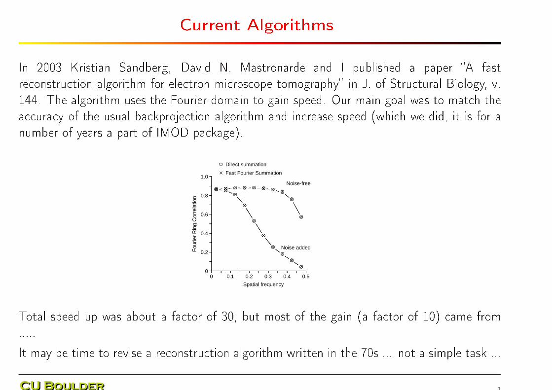
In 2003 Kristian Sandberg, David N. Mastronarde and I published a paper �A fastre onstru tion algorithm for ele tron mi ros ope tomography� in J. of Stru tural Biology, v.144. The algorithm uses the Fourier domain to gain speed. Our main goal was to mat h thea ura y of the usual ba kproje tion algorithm and in rease speed (whi h we did, it is for anumber of years a part of IMOD pa kage).0 0.1 0.2 0.3 0.4 0.5

Spatial frequency

0

0.2

0.4

0.6

0.8

1.0

Fou

rier

Rin

g C

orre

latio

n

Direct summation

Fast Fourier Summation

Noise-free

Noise added

Total speed up was about a fa tor of 30, but most of the gain (a fa tor of 10) ame from.....It may be time to revise a re onstru tion algorithm written in the 70s ... not a simple task ...1

Challenges of Ele tron Mi ros ope Tomography

1. The imaging te hnique is hardly �non-destru tive�; a limited useful energy range.2. Limited aperture resulting in artifa ts, very noisy data3. Di� ulties with forward modeling4. ....Currently we are looking at a number of new mathemati al tools to address several hallengesof NDE imaging in general and ele tron mi ros opy in parti ular.The rest of my talk is a mathemati al desription of our approa h and tools at our disposal.This work involves Kristian Sandberg, Lu as Monzón, Christopher Kur z and (re ently) MattReynolds.

2

Fourier transform on a �nite domain

It is well-known that a fun tion with ompa tly supported Fourier transform annot have ompa t support itself unless it is identi ally zero.Yet, all measurements, being approximate, violate this lo alization onstraint sin e we neverdeal with either in�nite bandwidth nor with fun tions that extend inde�nitely in spa e ortime.This onstraint is easily over ome for a �nite a ura y. For example, onsider a Gaussianand set a threshold on the fun tion and its Fourier transform, thus limiting both supports forany �nite a ura y.Thus, it is natural to analyze the operator whose e�e t on a fun tion is to trun ate it bothin spatial and Fourier domains. This has been the topi of a series of seminal papers bySlepian et al. ( ir a 1961), where it is observed (inter alia) that the eigenfun tions of su hoperator on a �nite interval are the Prolate Spheroidal Wave Fun tions (PSWFs) of lassi almathemati al physi s.

3

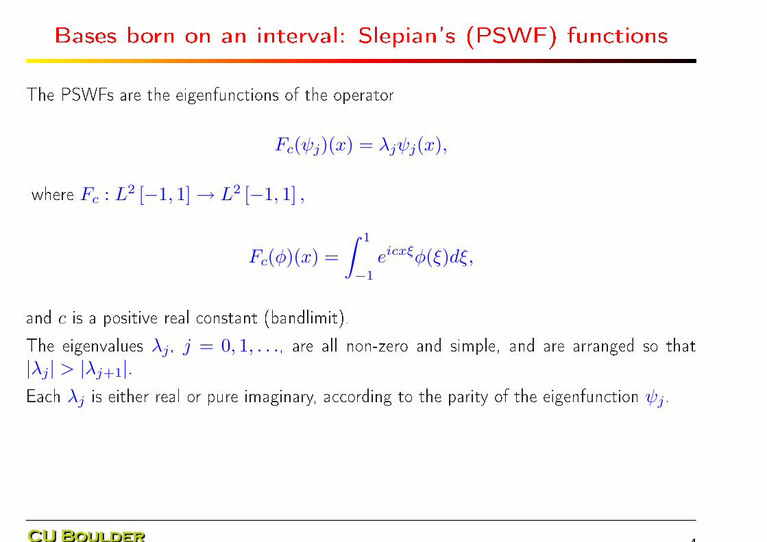
Bases born on an interval: Slepian's (PSWF) fun tions

The PSWFs are the eigenfun tions of the operator

Fc(ψj)(x) = λjψj(x),where Fc : L2 [−1, 1] → L2 [−1, 1] ,

Fc(φ)(x) =

∫ 1

−1

eicxξφ(ξ)dξ,

and c is a positive real onstant (bandlimit).The eigenvalues λj, j = 0, 1, . . ., are all non-zero and simple, and are arranged so that

|λj| > |λj+1|.Ea h λj is either real or pure imaginary, a ording to the parity of the eigenfun tion ψj.4

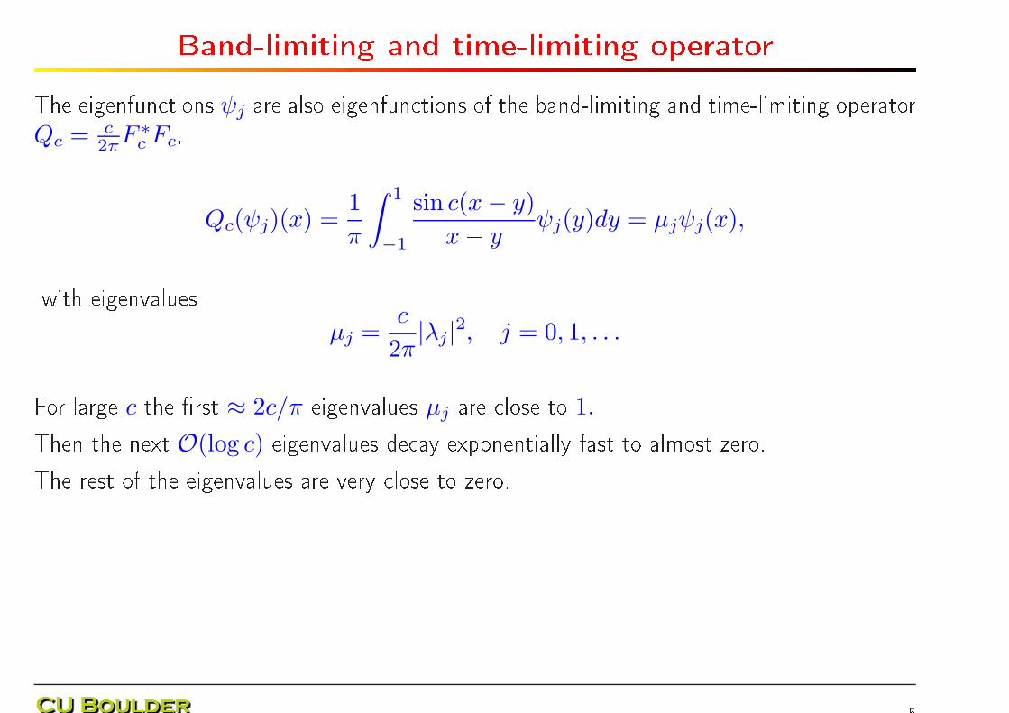
Band-limiting and time-limiting operatorThe eigenfun tions ψj are also eigenfun tions of the band-limiting and time-limiting operatorQc = c

2πF∗c Fc,

Qc(ψj)(x) =1

π

∫ 1

−1

sin c(x− y)

x− yψj(y)dy = µjψj(x),

with eigenvalues

µj =c

2π|λj|2, j = 0, 1, . . .

For large c the �rst ≈ 2c/π eigenvalues µj are lose to 1.Then the next O(log c) eigenvalues de ay exponentially fast to almost zero.The rest of the eigenvalues are very lose to zero.

5

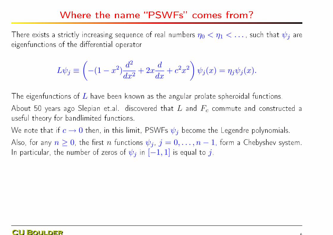
Where the name �PSWFs� omes from?There exists a stri tly in reasing sequen e of real numbers η0 < η1 < . . . , su h that ψj areeigenfun tions of the di�erential operator

Lψj ≡(

−(1 − x2)d2

dx2+ 2x

d

dx+ c2x2

)

ψj(x) = ηjψj(x).

The eigenfun tions of L have been known as the angular prolate spheroidal fun tions.About 50 years ago Slepian et.al. dis overed that L and Fc ommute and onstru ted auseful theory for bandlimited fun tions.We note that if c→ 0 then, in this limit, PSWFs ψj be ome the Legendre polynomials.Also, for any n ≥ 0, the �rst n fun tions ψj, j = 0, . . . , n− 1, form a Chebyshev system.In parti ular, the number of zeros of ψj in [−1, 1] is equal to j.

6

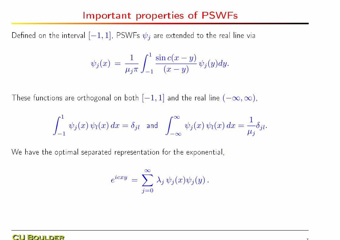
Important properties of PSWFsDe�ned on the interval [−1, 1], PSWFs ψj are extended to the real line viaψj(x) =

1

µjπ

∫ 1

−1

sin c(x− y)

(x− y)ψj(y)dy.

These fun tions are orthogonal on both [−1, 1] and the real line (−∞,∞),∫ 1

−1

ψj(x)ψl(x) dx = δjl and ∫ ∞

−∞ψj(x)ψl(x) dx =

1

µjδjl.

We have the optimal separated representation for the exponential,

eicxy =∞∑

j=0

λj ψj(x)ψj(y) .

7

Re ent results: Gaussian-type quadratures for bandlimitedfun tions

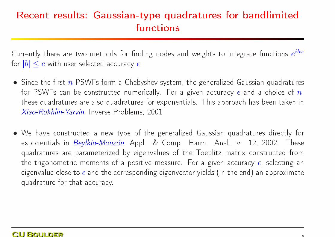
Currently there are two methods for �nding nodes and weights to integrate fun tions eibxfor |b| ≤ c with user sele ted a ura y ǫ:

• Sin e the �rst n PSWFs form a Chebyshev system, the generalized Gaussian quadraturesfor PSWFs an be onstru ted numeri ally. For a given a ura y ǫ and a hoi e of n,these quadratures are also quadratures for exponentials. This approa h has been taken inXiao-Rokhlin-Yarvin, Inverse Problems, 2001• We have onstru ted a new type of the generalized Gaussian quadratures dire tly forexponentials in Beylkin-Monzón, Appl. & Comp. Harm. Anal., v. 12, 2002. Thesequadratures are parameterized by eigenvalues of the Toeplitz matrix onstru ted fromthe trigonometri moments of a positive measure. For a given a ura y ǫ, sele ting aneigenvalue lose to ǫ and the orresponding eigenve tor yields (in the end) an approximatequadrature for that a ura y.

8

Distribution of nodes of Gaussian quadratures

50 100 150 200 2500.1

0.15

0.2

0.25

0.3

0.35

0.4

0.45

0.5

0.55

0.6

Number of nodes

Rat

io

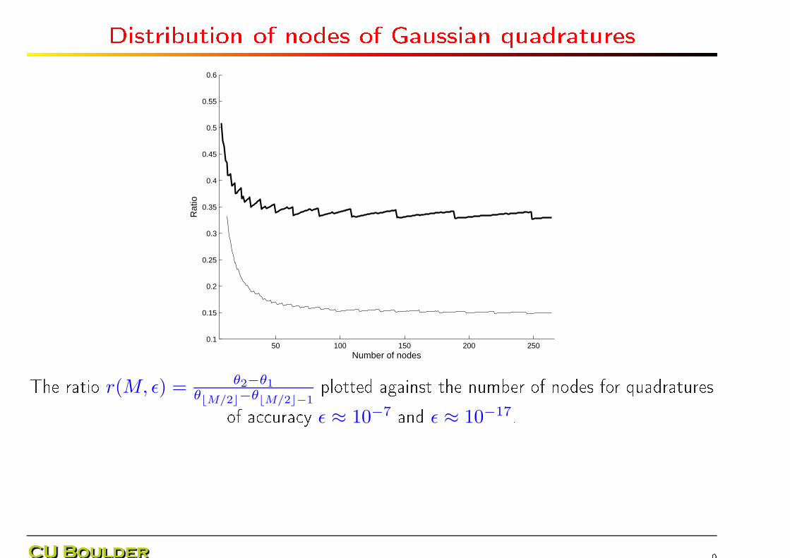
The ratio r(M, ǫ) = θ2−θ1θ⌊M/2⌋−θ⌊M/2⌋−1

plotted against the number of nodes for quadraturesof a ura y ǫ ≈ 10−7 and ǫ ≈ 10−17.

9

Sampling rate for Gaussian quadratures

50 100 150 200 2501

1.5

2

2.5

3

3.5

4

4.5

5

5.5

6

6.5

Number of nodes

Ove

rsam

plin

g fa

ctor

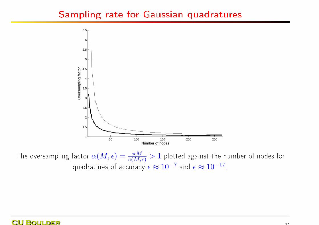
The oversampling fa tor α(M, ǫ) = πMc(M,ǫ) > 1 plotted against the number of nodes forquadratures of a ura y ǫ ≈ 10−7 and ǫ ≈ 10−17.

10

A ura y of the Gaussian quadratures50 100 150 200 250

−20

−18

−16

−14

−12

−10

−8

−6

−4

−2

0

Number of nodes

Err

or (

log 10

)

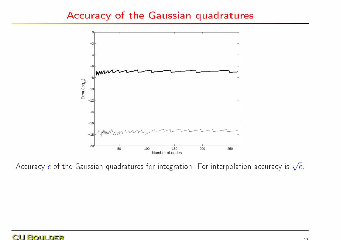
A ura y ǫ of the Gaussian quadratures for integration. For interpolation a ura y is √ǫ.11

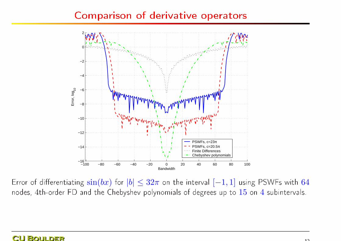
Comparison of derivative operators

−100 −80 −60 −40 −20 0 20 40 60 80 100−16

−14

−12

−10

−8

−6

−4

−2

0

2

Bandwidth

Err

or, l

og10

PSWFs, c=23πPSWFs, c=20.5πFinite DifferencesChebyshev polynomials

Error of di�erentiating sin(bx) for |b| ≤ 32π on the interval [−1, 1] using PSWFs with 64nodes, 4th-order FD and the Chebyshev polynomials of degrees up to 15 on 4 subintervals.12

Slepian fun tions in higher dimensions

Slepian (1964) also onsidered mapping of a disk in spa e to a disk in the Fourier domain(or a ball in higher dimension).

However, the spe trum of the spa e-limiting and band-limiting operator for the disk-to-diskmapping is substantially di�erent from that in 1D. Namely, the omplete spe trum has alarge transition region (of order O(N logN) out of O(N2) eigenvalues).

Re ently Yoel Shkolnisky implemented Slepian's onstru tion. For ea h angular mode thetransition region is O(logN), but there are O(N) angular modes!

13

Transforms from square in spa e to a disk in Fourierdomain (and ba k)

• A really long list of appli ations whi h in lude the Radon transform and its pra ti alvariants

• Note that the pseudo-polar DFT maps a square in spa e to a square in Fourier domainbut with a radial grid

• Dire tional bases, urvelets, et .Is there a � orre t� mathemati al obje t, an analogue of DFT, or this is just numeri s?What are �good� grids in a disk?

14

Forward and adjoint transforms

Consider the Fourier transform of a fun tion f supported in B,f(p) = F2c[f ](p) =

∫

B

f(x)e−ix·pdx,

and restri t the support of f to the disk of radius 2 , so thatF2c : L2(B) → L2(D2c).We then onsider the adjoint transform

F∗2c[g](x) =

1

4π2

∫

D2c

g(p)eix·pdp,

and limit the support of the resulting fun tion to the square B, so that

F∗2c : L2(D2c) → L2(B).

15

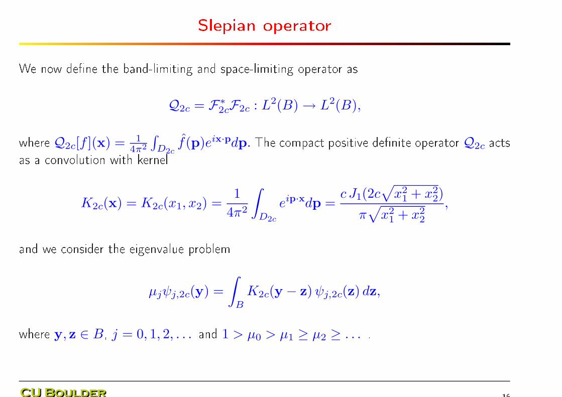
Slepian operator

We now de�ne the band-limiting and spa e-limiting operator asQ2c = F∗

2cF2c : L2(B) → L2(B),where Q2c[f ](x) = 14π2

∫

D2cf(p)eix·pdp. The ompa t positive de�nite operator Q2c a tsas a onvolution with kernel

K2c(x) = K2c(x1, x2) =1

4π2

∫

D2c

eip·xdp =c J1(2c

√

x21 + x2

2)

π√

x21 + x2

2

,

and we onsider the eigenvalue problemµjψj,2c(y) =

∫

B

K2c(y − z)ψj,2c(z) dz,

where y, z ∈ B, j = 0, 1, 2, . . . and 1 > µ0 > µ1 ≥ µ2 ≥ . . . .

16

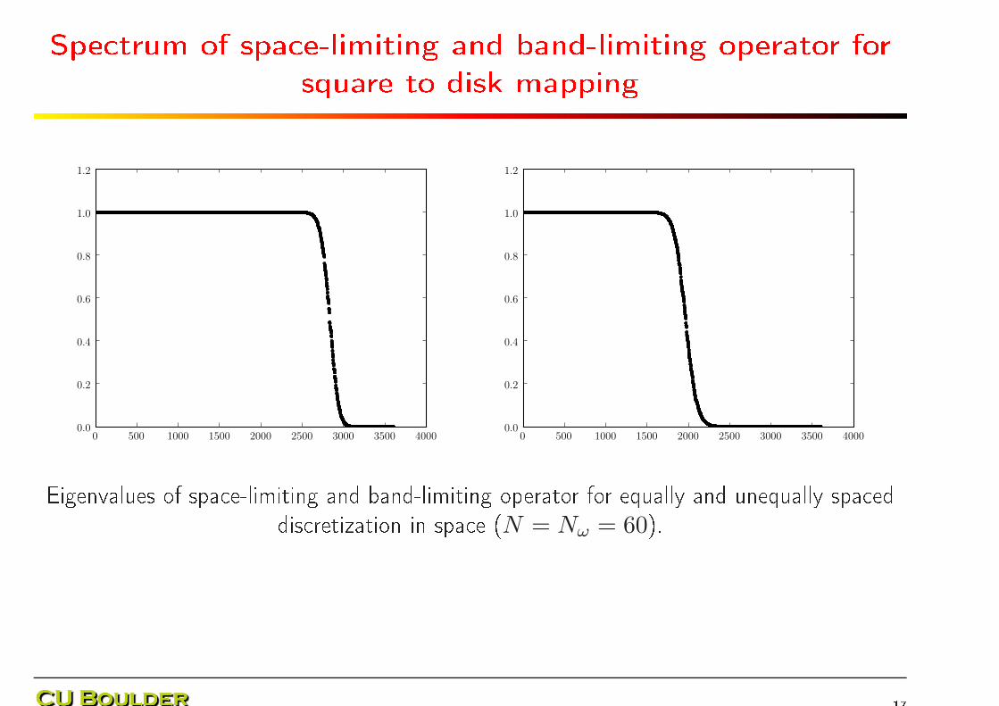
Spe trum of spa e-limiting and band-limiting operator forsquare to disk mapping

Eigenvalues of spa e-limiting and band-limiting operator for equally and unequally spa eddis retization in spa e (N = Nω = 60).

17

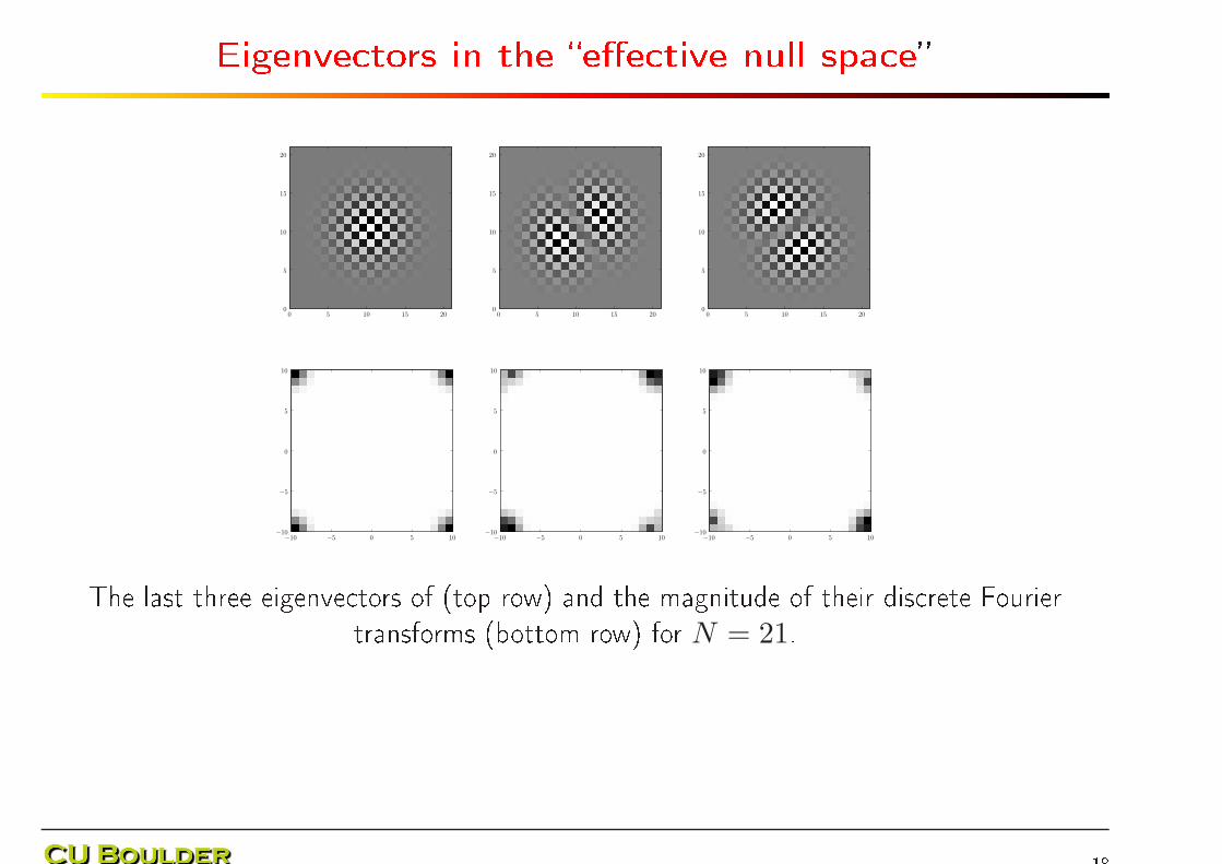
Eigenve tors in the �e�e tive null spa e�

The last three eigenve tors of (top row) and the magnitude of their dis rete Fouriertransforms (bottom row) for N = 21.

18

Quadratures: nodes and weights on the diameter of the disk

We ompute for given ǫ > 0 and bandlimit 2√

2c > 0 the nodes |ρk| < 1 and the weightswk > 0, k = 1, . . . ,M , where M = M(c, ǫ), su h that for all y ∈ [−1, 1]

∣

∣

∣

∣

∣

∫ 1

−1

ei 2√

2cρy |ρ| dρ−M∑

k=1

wkei 2

√2cρky

∣

∣

∣

∣

∣

≤ πǫ

c2.

With these we obtain a dis retization of the kernel,K2c(x) =

c2

π2

∫ 2π

0

∫ 1

0

ei 2c ρ(x1 cos θ+x2 sin θ)ρ dρ dθ

=c2

2π2

∫ 2π

0

(∫ 1

−1

ei 2c ρ(x1 cos θ+x2 sin θ)|ρ| dρ)

dθ.

19

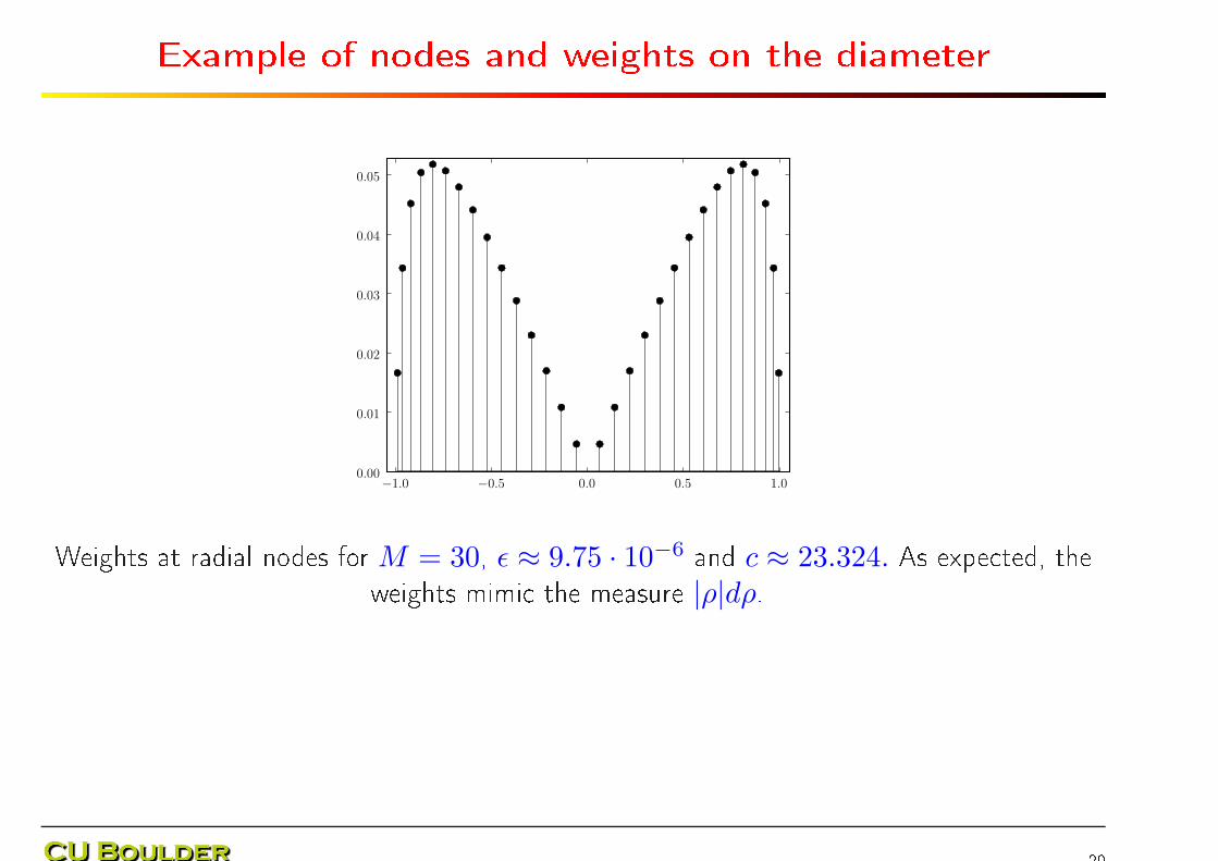
Example of nodes and weights on the diameter

Weights at radial nodes for M = 30, ǫ ≈ 9.75 · 10−6 and c ≈ 23.324. As expe ted, theweights mimi the measure |ρ|dρ.

20

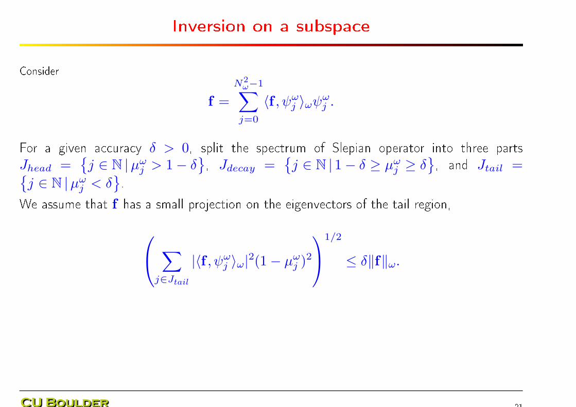
Inversion on a subspa e

Consider

f =

N2ω−1∑

j=0

〈f , ψωj 〉ωψω

j .

For a given a ura y δ > 0, split the spe trum of Slepian operator into three parts

Jhead ={

j ∈ N |µωj > 1 − δ

}, Jdecay ={

j ∈ N | 1 − δ ≥ µωj ≥ δ

}, and Jtail ={

j ∈ N |µωj < δ

}.We assume that f has a small proje tion on the eigenve tors of the tail region,

∑

j∈Jtail

|〈f , ψωj 〉ω|2(1 − µω

j )2

1/2

≤ δ‖f‖ω.

21

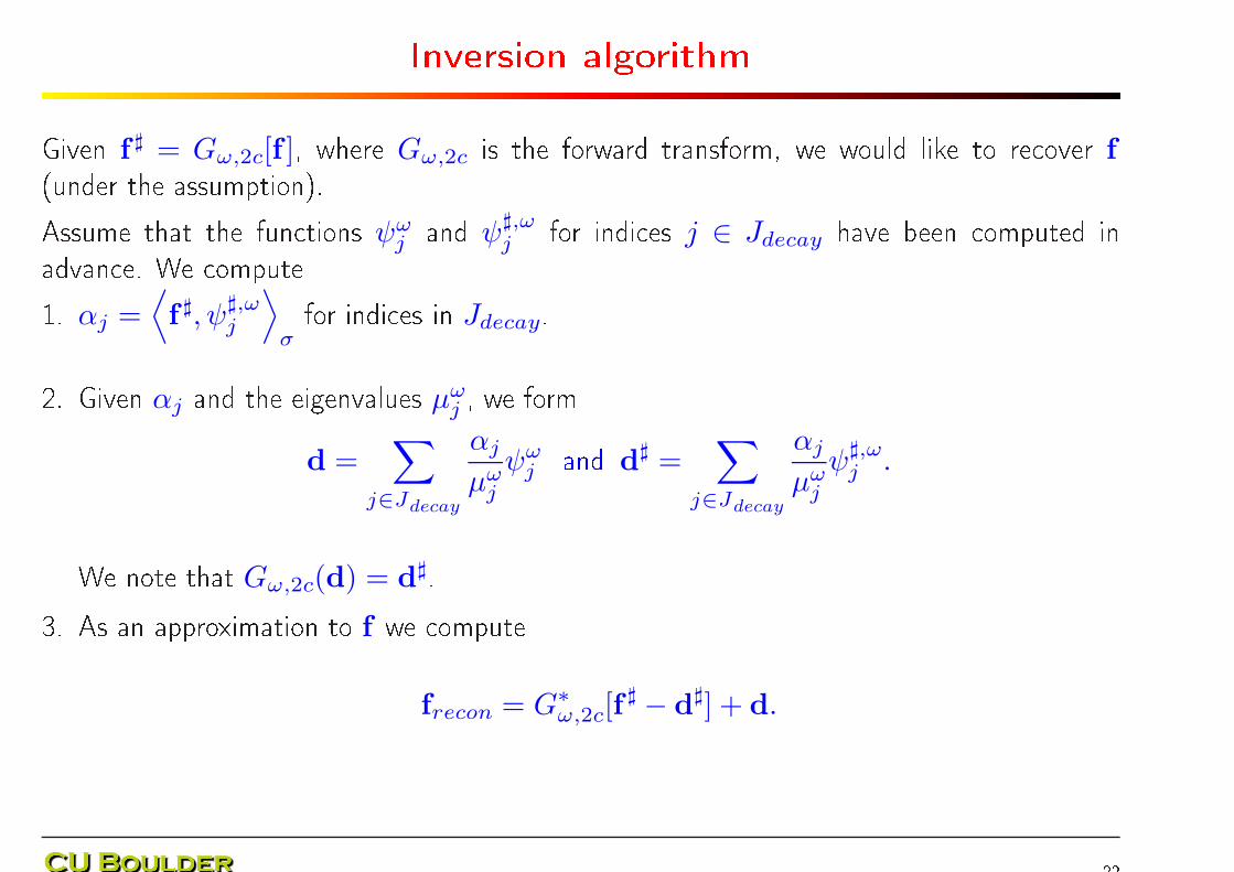
Inversion algorithm

Given f ♯ = Gω,2c[f ], where Gω,2c is the forward transform, we would like to re over f(under the assumption).Assume that the fun tions ψωj and ψ♯,ω

j for indi es j ∈ Jdecay have been omputed inadvan e. We ompute1. αj =⟨

f ♯, ψ♯,ωj

⟩

σ

for indi es in Jdecay.2. Given αj and the eigenvalues µωj , we form

d =∑

j∈Jdecay

αj

µωj

ψωj and d♯ =

∑

j∈Jdecay

αj

µωj

ψ♯,ωj .

We note that Gω,2c(d) = d♯.3. As an approximation to f we omputefrecon = G∗

ω,2c[f♯ − d♯] + d.

22

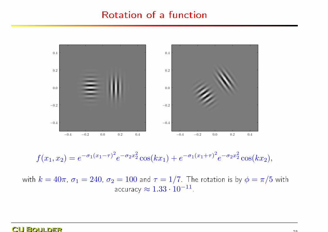
Rotation of a fun tionf(x1, x2) = e−σ1(x1−τ)2e−σ2x2

2 cos(kx1) + e−σ1(x1+τ)2e−σ2x22 cos(kx2),with k = 40π, σ1 = 240, σ2 = 100 and τ = 1/7. The rotation is by φ = π/5 witha ura y ≈ 1.33 · 10−11.

23

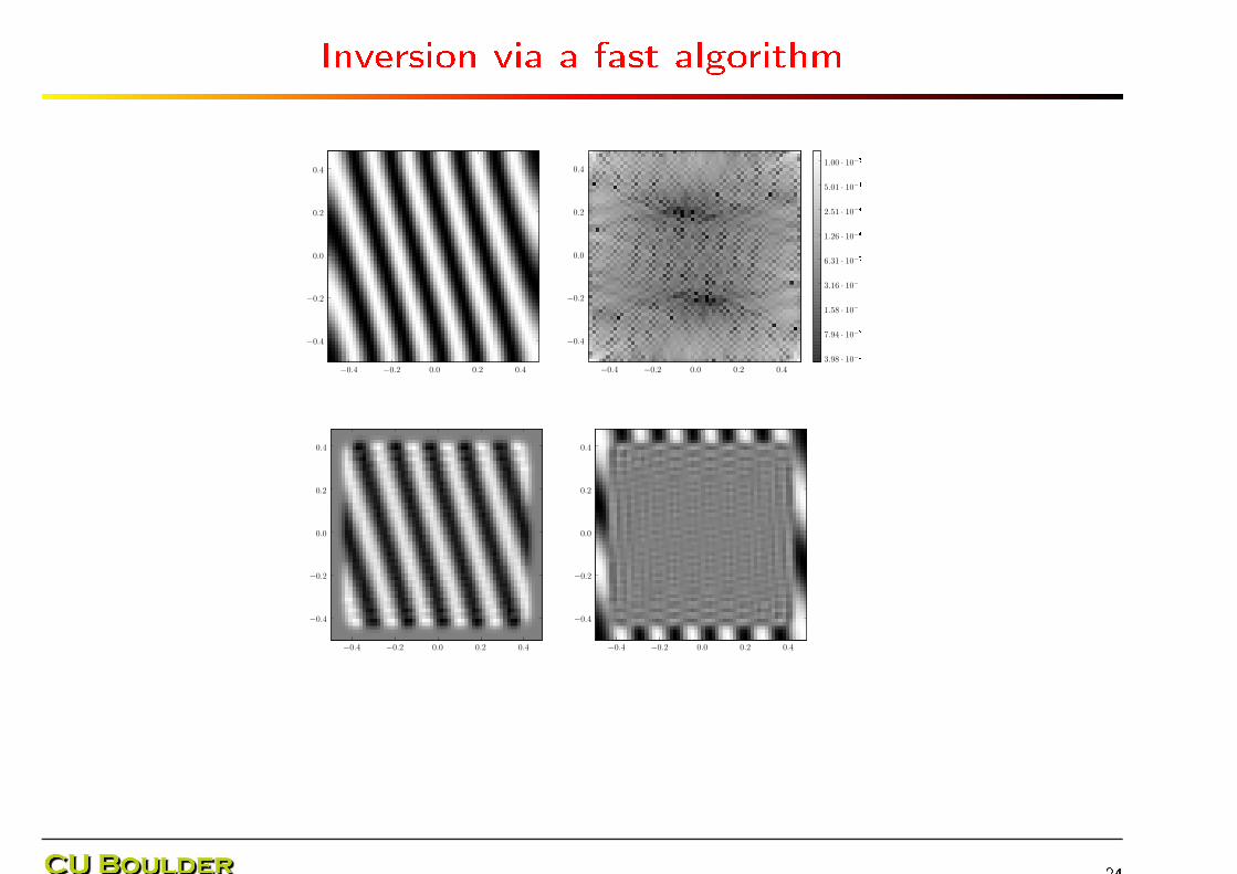
Inversion via a fast algorithm

24

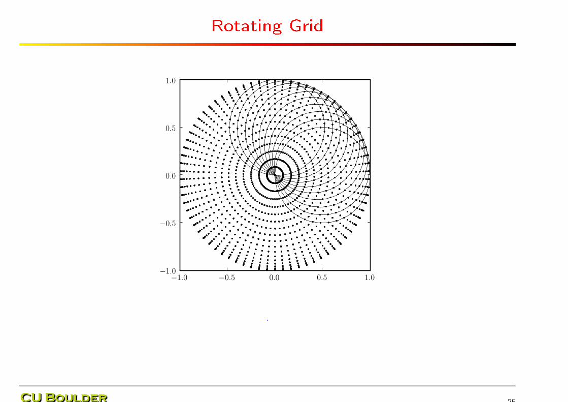
Rotating Grid.

25

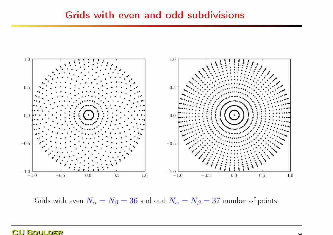
Grids with even and odd subdivisions

Grids with even Nα = Nβ = 36 and odd Nα = Nβ = 37 number of points.26

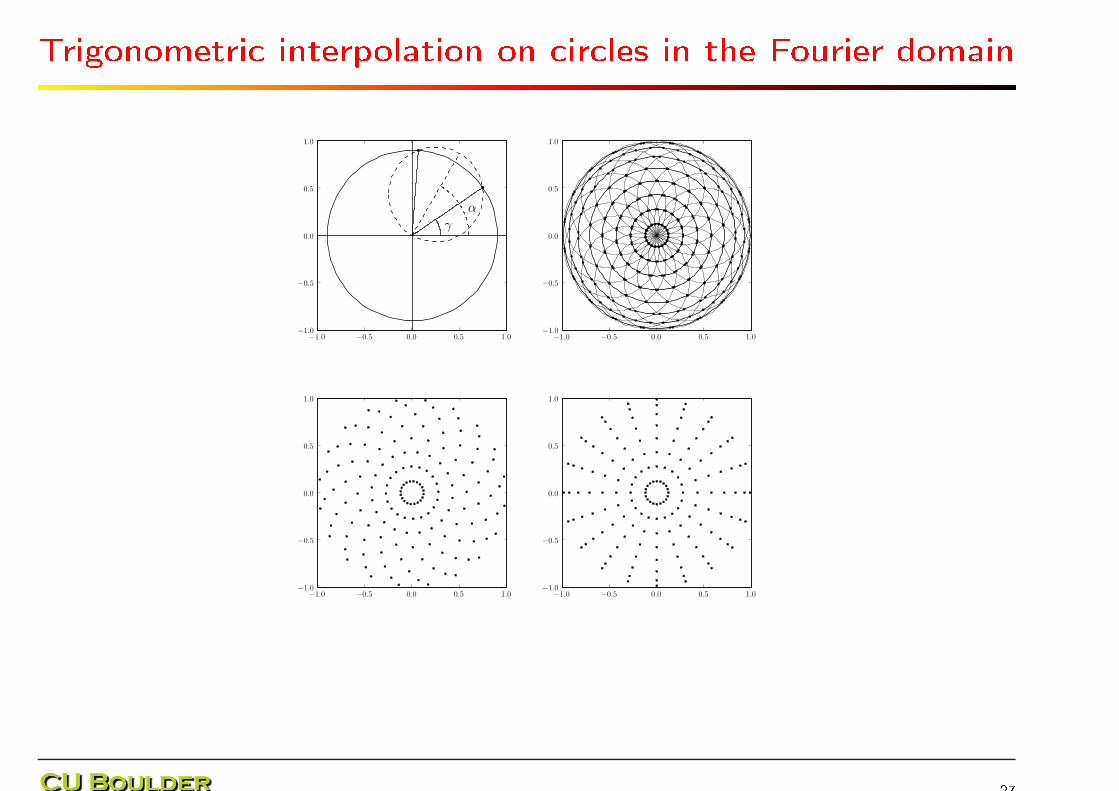
Trigonometri interpolation on ir les in the Fourier domain27

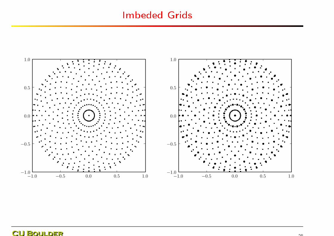
Imbeded Grids

28

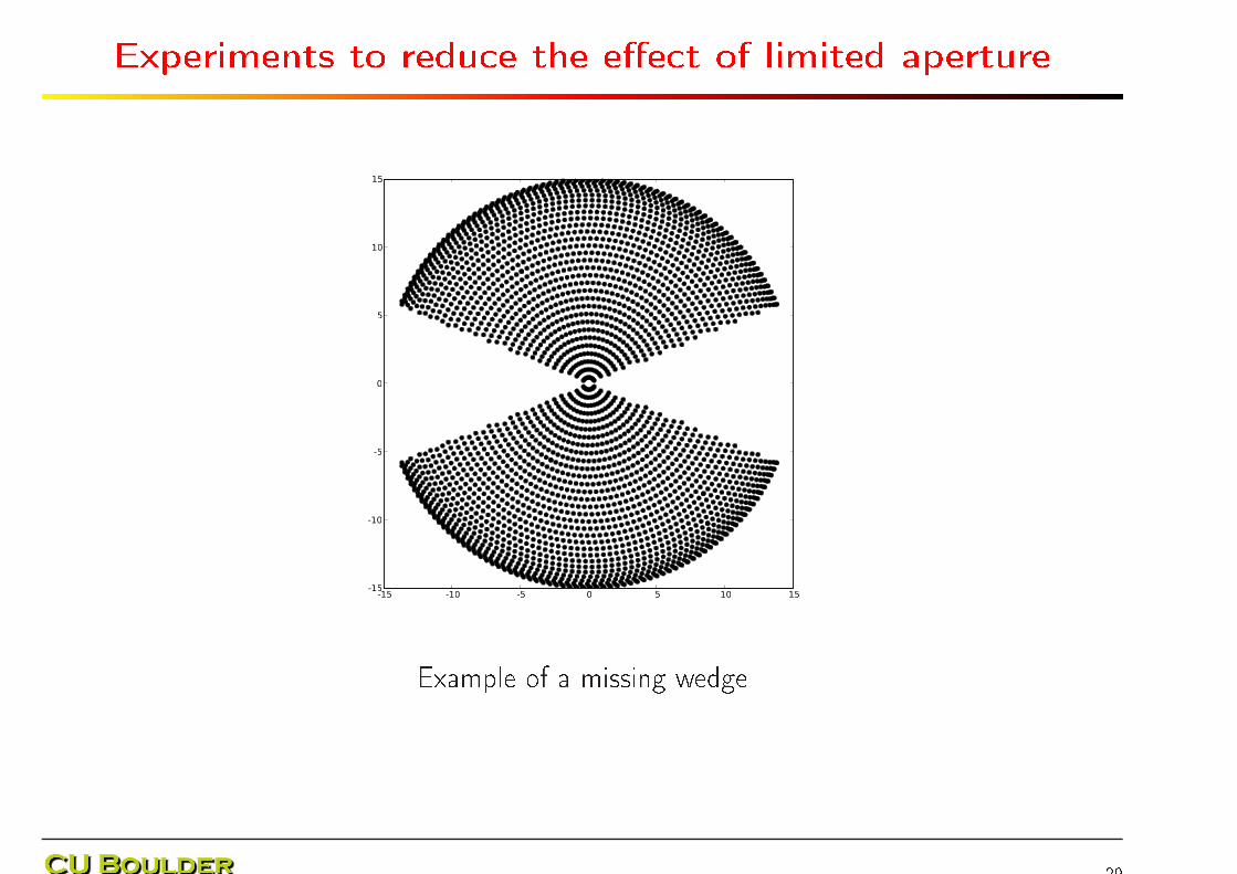
Experiments to redu e the e�e t of limited aperture

-15 -10 -5 0 5 10 15-15

-10

-5

0

5

10

15

Example of a missing wedge

29

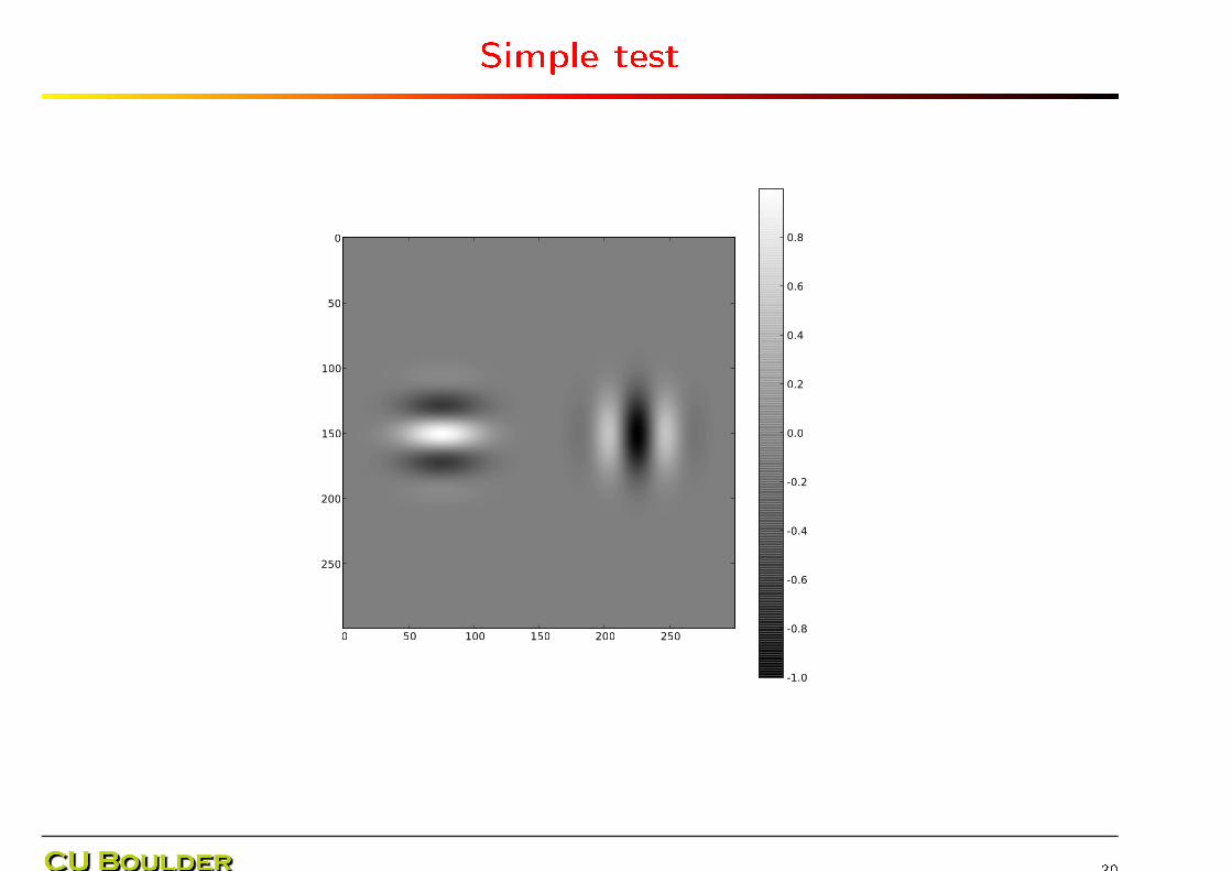
Simple test0 50 100 150 200 250

0

50

100

150

200

250

-1.0

-0.8

-0.6

-0.4

-0.2

0.0

0.2

0.4

0.6

0.8

30

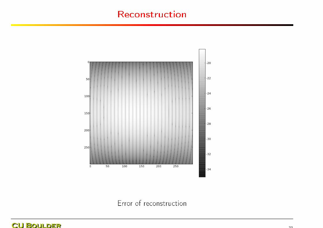
Re onstru tion0 50 100 150 200 250

0

50

100

150

200

250

-34

-32

-30

-28

-26

-24

-22

-20

Error of re onstru tion

31

Final remarks

Further work:

• Using these new transforms in pra ti al algorithms (MRI, Ele tron mi ros opy, ...). Notan obvious or easy task!

• 3D: dis retization of the sphere, rotating spheres, et .• Dire tional bases suitable for numeri al appli ations• Near optimal grids in �arbitrary� domains for fun tions bandlimited in a disk

32