University of Nebraska - LincolnDigitalCommons@University of Nebraska - Lincoln

USGS Staff -- Published Research US Geological Survey

2017

Greater Sage-Grouse Population Trends AcrossWyomingDavid R. EdmundsColorado State University - Fort Collins, dave.edmunds@rams.colostate.ed

Cameron L. AldridgeColorado State University - Fort Collins

Michael S. O'DonnellFort Collins Science Center

Adrian P. MonroeColorado State University - Fort Collins

Follow this and additional works at: https://digitalcommons.unl.edu/usgsstaffpub

Part of the Geology Commons, Oceanography and Atmospheric Sciences and MeteorologyCommons, Other Earth Sciences Commons, and the Other Environmental Sciences Commons

This Article is brought to you for free and open access by the US Geological Survey at DigitalCommons@University of Nebraska - Lincoln. It has beenaccepted for inclusion in USGS Staff -- Published Research by an authorized administrator of DigitalCommons@University of Nebraska - Lincoln.

Edmunds, David R.; Aldridge, Cameron L.; O'Donnell, Michael S.; and Monroe, Adrian P., "Greater Sage-Grouse Population TrendsAcross Wyoming" (2017). USGS Staff -- Published Research. 1035.https://digitalcommons.unl.edu/usgsstaffpub/1035

Research Article

Greater Sage-Grouse Population TrendsAcross Wyoming

DAVID R. EDMUNDS ,1 Natural Resource Ecology Laboratory, Colorado State University, in Cooperation With the U.S. Geological Survey, FortCollins Science Center, 2150 Centre Avenue, Building C, Fort Collins, CO 80526, USA

CAMERON L. ALDRIDGE , Natural Resource Ecology Laboratory and Department of Ecosystem Science and Sustainability, Colorado StateUniversity, in Cooperation With the U.S. Geological Survey, Fort Collins Science Center, 2150 Centre Avenue, Building C, Fort Collins, CO 80526,USA

MICHAEL S. O’DONNELL , U.S. Geological Survey, Fort Collins Science Center, 2150 Centre Avenue, Building C, Fort Collins, CO 80526, USA

ADRIAN P. MONROE , Natural Resource Ecology Laboratory, Colorado State University, in Cooperation With the U.S. Geological Survey, FortCollins Science Center, 2150 Centre Avenue, Building C, Fort Collins, CO 80526, USA

ABSTRACT The scale at which analyses are performed can have an effect on model results and often onescale does not accurately describe the ecological phenomena of interest (e.g., population trends) for wide-ranging species: yet, most ecological studies are performed at a single, arbitrary scale. To best determine localand regional trends for greater sage-grouse (Centrocercus urophasianus) in Wyoming, USA, we modeleddensity-independent and -dependent population growth across multiple spatial scales relevant tomanagement and conservation (Core Areas [habitat encompassing approximately 83% of the sage-grousepopulation on�24% of surface area in Wyoming], local Working Groups [7 regional areas for which groupsof local experts are tasked with implementingWyoming’s statewide sage-grouse conservation plan at the locallevel], Core Area status (Core Area vs. Non-Core Area) by Working Groups, and Core Areas by WorkingGroups). Our goal was to determine the influence of fine-scale population trends (Core Areas) on larger-scalepopulations (Working Group Areas). We modeled the natural log of change in population size (�x peakM lekcounts) by time to calculate the finite rate of population growth (l) for each population of interest from 1993to 2015.We found that in general when Core Area status (Core Area vs. Non-Core Area) was investigated byWorking Group Area, the 2 populations trended similarly and agreed with the overall trend of the WorkingGroup Area. However, at the finer scale where Core Areas were analyzed separately, Core Areas within thesame Working Group Area often trended differently and a few large Core Areas could influence the overallWorking Group Area trend and mask trends occurring in smaller Core Areas. Relatively close fine-scalepopulations of sage-grouse can trend differently, indicating that large-scale trends may not accurately depictwhat is occurring across the landscape (e.g., local effects of gas and oil fieldsmay bemasked by increasing largerpopulations). Published 2017. This article is a U.S. Government work and is in the public domain in the USA.

KEY WORDS Centrocercus urophasianus, density-dependent growth, density-independent growth, finite populationgrowth rate, generalized linear model, greater sage-grouse, population viability analysis, Wyoming.

The scale at which analyses are performed can influencemodel outcomes because results will differ across scales(Bissonette 2017). There is no single scale to accurately andcompletely describe ecological phenomena (e.g., populationtrends) and therefore multiple spatial scales are required toaccurately evaluate populations (Fuhlendorf et al. 2002,Bissonette 2017). For wide-ranging species, evaluatingpopulation trends at a single scale may result in anincomplete interpretation of population change (Fuhlendorfet al. 2002). Modeling population trends at multiple spatialscales also can facilitate the determination of the cause of

population changes and be used to prioritize conservationstrategies and research (Sadoul 1997, DeSante et al. 2001,Wallace et al. 2010). However, many studies are performedarbitrarily at single spatial scales and few researchers haveevaluated the relationship between scale and populationtrends (Bissonette 1997, 2017; Fuhlendorf et al. 2002).Greater sage-grouse (Centrocercus urophasianus; sage-

grouse) currently occupy roughly 56% of their historicalrange in western North America, which now includesportions of 11 states in the United States and 2 Canadianprovinces but previously encompassed 15 states and 3provinces (Connelly and Braun 1997, Schroeder et al. 2004).Range contraction has been linked to loss of habitat in thesagebrush (Artemisia spp.) ecosystem (Schroeder et al. 2004),for which sage-grouse are an obligate species (Beever andAldridge 2011). Landscape changes of sagebrush ecosystems

Received: 22 May 2017; Accepted: 10 September 2017

1E-mail: dave.edmunds@rams.colostate.ed

The Journal of Wildlife Management; DOI: 10.1002/jwmg.21386

Edmunds et al. � WY Sage-Grouse Population Viability Analysis 1

have been linked to livestock grazing (Beck and Mitchell2000, Hayes and Holl 2003, Crawford et al. 2004), oil andgas development (Braun et al. 2002, Lyon and Anderson2003, Holloran 2005), cultivation (Connelly et al. 2004),invasive plant species (e.g., cheatgrass [Bromus tectorum];Wisdom et al. 2002, Knick et al. 2003, Connelly et al. 2004),and changes in fire regime (Connelly et al. 2000, 2004).In addition to range contraction, sage-grouse populations

generally have been declining range-wide since the 1920s(Braun 1998). Sage-grouse populations fluctuate overapproximately 9- to 10-year cycles (Fedy and Aldridge2011, Fedy and Doherty 2011), whereby periods of declineare followed by periods of increasing populations and viceversa (Rich 1985); however, subsequent population highsgenerally are lower than the preceding high level, resulting inan overall downward population trend (Braun 1998). Therange-wide breeding population has declined 45–80% sincethe 1950s with the majority of declines occurring after 1980(Braun 1998). Others have estimated breeding populationsdeclined approximately 2% annually during 1965–2003(Connelly et al. 2004). Of note, these studies occurred >13years ago, and there is some uncertainty regarding morerecent population trends. Population declines have resultedin sage-grouse populations in Canada being listed asendangered by the Committee on the Status of EndangeredWildlife in Canada (Aldridge and Brigham 2003) andrecently, the United States Fish and Wildlife Service(USFWS) considered listing sage-grouse under the Endan-gered Species Act but ruled sage-grouse were not warrantedfor protection (USFWS 2015). This ruling was based onunprecedented conservation efforts that were implementedin federal and state management plans written during theprevious 5 years targeted at ameliorating population threatsidentified by the USFWS when they ruled that sage-grousewere warranted for listing in 2010 but precluded because ofhigher priority species (USFWS 2010).The state of Wyoming contains approximately 37% of the

remaining sage-grouse populations (Doherty et al. 2010).However, populations of sage-grouse in Wyoming aredeclining (Fedy and Aldridge 2011). Populations across thestate declined 29–76% during 2007–2013, resulting inpopulations that represented approximately 4–25% of thesize of the same populations in the 1970s and 1980s (Gartonet al. 2011, 2015). Further, gas and oil development hascaused lek abandonment and declines in breeding popula-tions (Green et al. 2017), particularly in western andnortheast Wyoming (Holloran 2005, Walker et al. 2007).The period 2007–2013 appears to have encompassed the

low end of the approximately 10-year cycle that perhapsended in 2013, so population declines may have beenexacerbated by the declining period in the population cycle.However, the last 3 decadal cycles have resulted in decreasesin the magnitude of change between periods of highs andlows, resulting in an overall population decline andpopulations reaching the lowest range-wide estimate(48,641 males) since the 1960s when counting males onspring breeding grounds, or leks, began in earnest (Gartonet al. 2011, 2015). This suggests populations should rebound,

but low annual turnover and reproductive rates indicatepopulation recovery may be slow (Connelly and Braun 1997).Furthermore, models forecasting future oil and gas, wind,and residential development in Wyoming project futurepopulation declines of 9–29% in Wyoming populations overlong-term scenarios (Copeland et al. 2013), with measureddeclines of up to 15%/year estimated for current high-densitydevelopments (Green et al. 2017).Sage-grouse are an indicator species of the overall health of

sagebrush ecosystems (Connelly et al. 2004, Blomberg et al.2013), which are one of the most imperiled ecosystems inNorth America (Noss et al. 1995). Bird species endemic toshrublands and grasslands are declining at quicker rates thanany other species assemblage in North America (Knick et al.2003). Sage-grouse may serve as an umbrella species, wherebymanagement strategies for one species benefit co-occurringendemic species (Branton and Richardson 2011), such aspasserine species (Rowland et al. 2006, Hanser and Knick2011). Furthermore, recent evidence demonstrates thatconservation of umbrella species results in higher speciesrichness and abundance of co-occurring species when birds arethe umbrella species (Branton and Richardson 2011). Withsage-grouse populations decreasing, it is imperative to assesstheir population trends based on boundaries highlightinglandscape changes and spatial variability of the populations.Sage-grouse leks are traditional display areas where �2

male sage-grouse gather annually (or�2 years in the previous5) in the spring to attract female mates and usually are locatedin open areas that are within or directly adjacent to sagebrushhabitats (Connelly et al. 2011b). The consistent location oflek sites makes them ideal sites for population monitoringand counting males at leks (i.e., lek counts) has been usedtraditionally by state and provincial wildlife agencies as anindex of population abundance (Walsh et al. 2004, Connellyet al. 2011a). Recently it has been questioned if lek counts areappropriate to use as accurate indicators of population trends(Walsh et al. 2004); however, Dahlgren et al. (2016)determined male lek counts were appropriate to use as anindex of population change. Further, Blomberg et al. (2013)concluded lek counts were well suited for estimatingpopulation growth rates across multi-year intervals andmultiple studies have used them in this way (Walker et al.2007, Garton et al. 2011, Dahlgren et al. 2016, Monroe et al.2016, Green et al. 2017).WyomingGame and Fish Department (WGFD)Working

Group Areas (WGFD 2003) were established in 2003 toallow local working groups, comprised of up to 12 individualsknowledgeable in or from diverse areas such as agriculture,conservation, industry, and natural resource agencies, toimplement Wyoming’s statewide sage-grouse conservationplan at the local level (WGFD 2003). Wyoming CorePopulation Areas (Core Areas) are habitat designationsencompassing approximately 83% of the sage-grousepopulation on approximately 24% of surface area inWyoming; protection of these areas from disturbance isintended to maintain viable sage-grouse populations inWyoming (State of Wyoming 2015). In 2008, the USFWSsupported Wyoming’s Core Population Areas strategy,

2 The Journal of Wildlife Management � 9999()

stating that it was a sound policy to conserve Wyoming’ssage-grouse populations if implemented as written (USFWS2015). The goal of the Core Area strategy was, “ . . . tominimize future disturbance by co-locating proposeddisturbances within areas already disturbed or naturallyunsuitable” (State of Wyoming 2015).We assessed population trends of sage-grouse in Wyoming

by incorporating lek count data across 23 years (1993–2015)into a population viability analysis (PVA) with density-independent (Dennis et al. 1991) and -dependent (Gartonet al. 2011) population models to calculate the finite rate ofpopulation growth (l) within multiple management delin-eations. We hypothesized that management-defined pop-ulations declined (l< 1.0) during the study period and thetrend in l would differ for populations evaluated at multiplespatial scales (i.e., Core Areas by Working Group Area andCore Area status by Working Group Area). We investigatedpopulation trends across multiple spatial scales to determinethe influence of fine-scale population trends (Core Areas) onlarger-scale populations (Working Group Areas) and todetermine if population trends of leks located within CoreAreas varied from leks located outside of Core Areas.

STUDY AREA

Our study region encompassed the Wyoming distributionof current sage-grouse range (Christiansen and Whitford2015) located within sagebrush communities, which coveredapproximately 150,000 km2, or roughly 66% of the state(Beetle and Johnson 1982).WithinWyoming, the sagebrush-steppecommunities aredominatedbyWyomingbig sagebrush(A. tridentata wyomingensis; Cagney et al. 2010). Wyoming issemiarid and generally has long, cold winters and short, coolsummers with themajority of precipitation occurring in springand early summer. Average maximum temperature in lowerbasins in July ranged between 298C and 358C and averageminimum temperature in January ranged between�128C and�208C depending on the region (Western Regional ClimateCenter [WRCC] 2016). Precipitation varies widely byelevation, topography, and region, but usually the majorityfalls in the mountains, whereas surrounding basins remainmuch drier (WRCC 2016). Elevation at evaluated lek sitesaveraged 1,824m and ranged from 1,093–2,535m. The sage-grouse range was divided into 7 Working Group Areasdistributed throughout the state, which were designated tohelp implementWyoming’s Greater Sage-Grouse Conserva-tion Plan based on recommendations from local workinggroups (WGFD 2003). A portion of the range was furtherdivided into 27 Core Areas where disturbance was limited byspecial protections for these leks as part of the conservationefforts to help prevent listing sage-grouse as threatened orendangered (State of Wyoming 2015). Core Area boundarieswere separate from and could overlap with Working GroupArea boundaries (Fig. 1).

METHODS

We used the Wyoming statewide lek count databasemaintained and provided by the WGFD for all analyses.The WGFD and partnering agencies conducted lek counts

with protocols approved byWGFD (Christiansen 2012). Thedatabase records date back to 1948, but we restricted counts to1993–2015 because the number of leks counted annually wasinsufficient for analyses prior to 1993; the results of analyseswere resilient to changing the startingandendingyears to1995and 2013, respectively, showing the choice in years did notsignificantly influence results (Table S1, available online inSupporting Information).We restricted the dates of counts to1 March–31 May to maximize probability of detecting peakmale lek counts (Fedy andAldridge2011) and timingof countsto 30 minutes pre-sunrise to 90 minutes post-sunrise tomaximize the number of leks included in analyses and increaseprecision of trend estimates (Monroe et al. 2016). We alsoremoved records that indicated weather conditions with windspeeds�16 km/hourorwhere precipitation occurred to ensureall counts followed standardized lek count procedures(Christiansen 2012, Monroe et al. 2016). We calculated thepeakmale lek count for all leks annually and then averaged thepeak male lek count across each population of interest,resulting in 1 average lek count per year (Monroe et al. 2016) toallow modeling of annual change in population size of countdata (Morris andDoak 2002).We added 0.5 to all average lekcounts to allow inclusion of mean counts of zero in analyses(Geissler and Noon 1981, Collins 1990, Monroe et al. 2016).We investigated population trends of sage-grouse in

Wyoming within multiple management delineations:Wyoming Game and Fish Department (WGFD) WorkingGroup Areas (WGFD 2003), Wyoming Core PopulationAreas (Core Areas; State of Wyoming 2015), Core Areas byWorking Group Area, and Core Area status (leks locatedwithin Core Areas [Core Areas] vs. leks located outside ofCore Areas [Non-Core Areas]) by Working Group Area.For Core Areas by Working Group Area and Core Areastatus byWorking Group Area groupings, where Core Areaswere located in>1Working Group Area, we assigned leks tothe specific Working Group Area in which they werelocated.

Statistical AnalysesPopulation viability analysis is a collection of methods thathas been used to quantitatively assess and forecast the mostlikely future status of a population or a group of relatedpopulations (Morris et al. 1999). Dennis et al. (1991)developed a simple linear regression-based method toperform PVAs and calculate population growth rates andextinction probabilities from time series data of populationabundance, including count data. Some have criticizedmethods developed by Dennis et al. (1991) for the use ofcount data in PVAs (e.g., Holmes 2001). However,criticisms have focused on the use of regression modelsfor the calculation of the probability of extinction or meantime to extinction, rather than the calculation of populationgrowth rates (Ludwig 1999, Fieberg and Ellner 2000, Reedet al. 2002, Wilcox and Possingham 2002). Holmes (2001)argued that population growth rate is a more useful riskmetric than the probability of extinction. Furthermore, themodel in Dennis et al. (1991) has received broad support(Morris et al. 1999, Morris and Doak 2002) and has been

Edmunds et al. � WY Sage-Grouse Population Viability Analysis 3

used widely to perform PVAs for a variety of species(Nicholls et al. 1996, Gerber et al. 1999, Schultz andHammond 2003, Walker et al. 2007, Blomberg et al. 2013).We regressed the natural logarithm (log) of annual change

in population size log Ntþ1

Nt

� �� �against time, to estimate the

intrinsic per capita rate of growth (r; Dennis et al. 1991,Morris and Doak 2002) assuming density-independentgrowth (exponential model), where r was the slope of theregression line. We employed a transformation for unequalvariances as an independent variable (xi) in all models(Morris and Doak 2002):

xi ¼ffiffiffiffiffiffiffiffiffiffiffiffiffiffiffiffiffitiþ1 � ti

p;

where ti is time in years. The dependent variable was (Morrisand Doak 2002)

yi ¼log Ntþ1

Nt

� �� �ffiffiffiffiffiffiffiffiffiffiffiffiffiffiffiffiffitiþ1 � ti

p :

We also modeled r with Ricker (Ricker 1954, Dennis andTaper 1994) and Gompertz (Jacobson et al. 2004) growthmodels assuming density-dependent growth and using thesame dependent variable as for the exponential model. Wespecified the Ricker form as

Ntþ1 ¼ Ntexp r þ bN t þ etð Þ;

where r is the estimated rate of population change, b is theslope estimate for density dependence, and et is annual error(Dennis and Taper 1994, Morris and Doak 2002). Similarly,the Gompertz form (Jacobson et al. 2004) is specified as

Ntþ1 ¼ Ntexp r þ b log Ntð Þ þ etð Þ:The Ricker model assumes a constant linear decrease of r as

the population size (Nt) increases. The Gompertz model,however, assumes a linear decrease in r as log Ntð Þ increases,resulting in a stronger density-dependent response to achange in population size. We used the glm function inprogram R (R Version 3.2.5, www.r-project.org, accessed

Figure 1. Core Population Areas (Core Areas), Wyoming Game and Fish Department Working Group Areas (labeled), and lek locations used in populationviability analyses for greater sage-grouse, Wyoming, USA, 1993–2015.

4 The Journal of Wildlife Management � 9999()

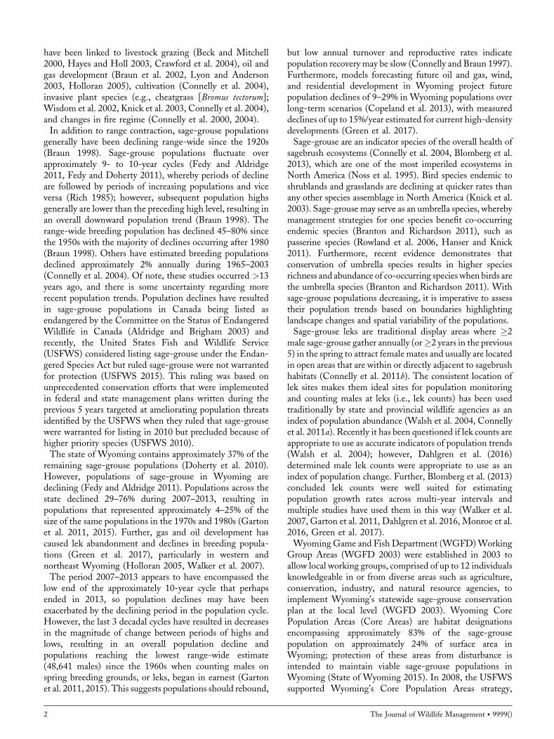
25 Apr 2016) to perform all modeling; the exponential modelstructure was based on the popbio package code (Version2.4.3, https://cran.r-project.org/web/packages/popbio/index.html, accessed 25 Apr 2016) following methods previouslydescribed (Monroe et al. 2016). The Ricker and Gompertzmodel structureswere based onRcode providedbyD.F.Doak(University of Colorado, personal communication) and tookthe model forms as shown above. We then transformed rinto l based on the conversion l ¼ er (Case 2000, Mills2013).Sage-grouse populations inWyoming cycle every 6–9 years

(Fedy and Aldridge 2011, Fedy and Doherty 2011); toaccount for these cycles, we attempted to de-trend the databy adding 2 different interval effect terms (see below)separately to each of the 3 models (exponential, Ricker, andGompertz). We evaluated 9 models for every populationwith adequate data by applying the 3 base models and the 3models with each of the 2 interval effects separately. The 2interval effect terms were based on the cycles present in ourreduced lek count data (1993–2015).We defined cycles usinga generalized additive model (GAM; Hastie and Tibshirani1990, Fewster et al. 2000, Wood 2006, Fedy and Aldridge2011) employed with the gam function of the mgcv package(Version 1.8-9, https://cran.r-project.org/web/packages/mgcv/index.html, accessed 03 Mar 2016) in program R.We determined years when the annual rate of change in theabundance index (Fewster et al. 2000) experienced astatistically significant upturn or downturn, defined aschange points, with the GAM analysis following methodspreviously described (Fig. 2; Fedy and Aldridge 2011). Weselected the years that marked the end of a trend in the cycle(top of peaks and bottom of valleys) from the change points(inflection points) to define intervals. The years 2000 and2006 marked the start of declining and the end of increasingintervals (peaks) and the years 1996, 2003, and 2013 markedthe start of increasing and the end of declining intervals(valleys; Fig. 2). We categorized years into numberedintervals (1–6) with the inflection point years marking thestart of the numbered intervals; we added the interval effectto models as a categorical covariate termed numberedinterval. Similarly, we categorized each year into increasingor decreasing intervals based on trends in the abundanceindex between inflection points; we added this interval effectas a covariate termed trend interval. We set the inflectionpoint years as the intercept (reference condition) in the glmto facilitate comparison of increasing and decreasing intervalsto the inflection points. For both interval effects models(numbered and trend), we calculated the overall growth rate(r) by averaging growth rates across all intervals (Mills 2013).Non-consecutive years of average peak male counts were

not permissible with the interval effect models because wecould not include a transformation to account for the unequalvariances associated with varying interval lengths, whichviolates the assumption of equal variances required forregression analysis (Morris and Doak 2002, Stubben andMilligan 2007). Furthermore, >1 year of data per intervalwas required to run the glm function and model selection

analysis (details below). After calculating Ntþ1

Nt

� �, we

removed values that were based on years (t) separated bytime lengths >1 to ensure equal length of time betweenconsecutive years; afterwards, we removed intervals (specifictrend or numbered intervals) that contained <2 years ofchange in population size data. If the removal criteriaresulted in <2 levels for the trend interval or numberedinterval effects, then we did not perform that specificanalysis. If processing resulted in <2 levels for the trendinterval and number interval effects, then we removed theinterval effect models from analysis for that population andanalyzed only the 3 base models with the original datasetprior to processing to maximize the number of years of dataused in analysis.We used Akaike’s Information Criterion (AIC) corrected

for small sample sizes (AICc) to select the top model for eachpopulation (Working Group Areas, Core Areas, Core Areasby Working Group Area, and Core Area Status by WorkingGroup Area; Burnham and Anderson 2010); we calculatedAICc values with the AICcmodavg R package (Version 2.0-4, https://cran.r-project.org/web/packages/AICcmodavg/index.html, accessed 13 Apr 2016). For populations with>1 supported model based on the difference in AICc valuefrom the lowest AICc value (DAICc < 2.0; Burnham andAnderson 2010), we used 10-fold cross-validation folded tothe maximum number of years of annual change inpopulation size data up to 10 years to calculate the bias-corrected prediction error for each model (James et al. 2013).We calculated the 10-fold cross-validation bias correctedprediction error with the boot R package (Version 1.3-18,

Figure 2. Overall lek trend model estimating abundance index fromgeneralized additive modeling of lek count data used in population viabilityanalyses for greater sage-grouse, Wyoming, USA, 1993–2015. We used thelek trend to define years where there were significant upturns (hollow circles)or downturns (black circles) in population cycles, defined as change points.Then we selected the years that marked the end of a trend in the cycle(inflection points) from the change points to define intervals. Peak years(black arrows) marked the start of declining and the end of increasingintervals and valley years (gray arrows) marked the start of increasing and theend of declining intervals. Dashed lines represent the 95% confidenceinterval.

Edmunds et al. � WY Sage-Grouse Population Viability Analysis 5

https://cran.r-project.org/web/packages/boot/index.html,accessed 25 Apr 2016). We selected the top models with thelowest prediction error using the competing models withDAICc< 2.0. We included our R code used to perform PVAin the supplemental material (Table S2, available online inSupporting Information).

RESULTS

We analyzed data from 1,556 of Wyoming’s 2,418documented leks after narrowing the lek count database toappropriate records (Fig. 1). We used 33,078 count recordsafter excluding counts conducted under unsuitable con-ditions. Two Core Areas, Bear River located within theSouthwest Working Group Area and Thermopolis locatedwithin the Bighorn Basin Working Group Area, lackedsufficient data to analyze Core Area-specific trends. Wecombined lek count data for the Thermopolis Core Areawith other Core Areas for analysis based on Core Status byWorking Group Area.Seven of the 8 Working Group Area top models included

the trend interval covariate. The Ricker and Gompertz trendinterval models were identified as the top model of 3different Working Group Areas each, whereas the exponen-tial trend interval model was identified as a top model for theseventh population (Table S3, available online in SupportingInformation). The exponential model was the top model forthe eighth population (Table S3). Population trend analysesfor the Working Group Areas showed that l< 1.0 for 6 outof 8 populations and l was different from 1.0 based on 95%confidence intervals for 5 of those 6 areas (Table 1). The 2populations with an increasing trend, but with confidenceintervals overlapping 1.0, were in the northwest part of thestate (Upper Snake River Basin and Bighorn Basin), whereasthe 2 populations in the southeast part of the state (BatesHole-Shirley Basin and South Central) declined at a smallbut significant rate (0.7% annual decline each; 95%CI¼ 0.986 to <1.000; Fig. 3). The remaining populationsdeclined between 4.5% and 29.6% annually (Fig. 3).For the Core Area populations, the 3 basic models without

interval covariates comprised the top models for 19 out of 32populations; the 3 trend interval models comprised the topmodels for 11 of the populations, and the top model for theSage Core Area population was the Gompertz numberedinterval model (Table S4, available online in SupportingInformation). Analyses for 24 of 31 Core Area populations

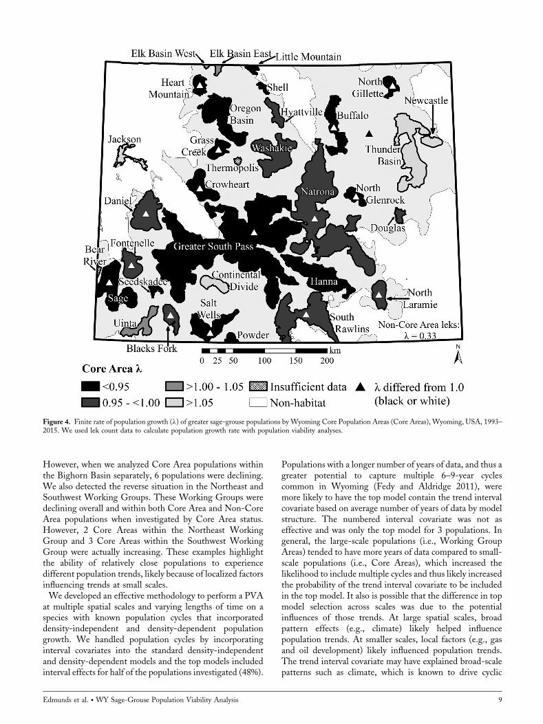
and the statewide Non-Core Area population showed thatl< 1.0 and of those, l differed from 1.0 for 15 Core Areapopulations and the Non-Core Area population based on95% confidence intervals (Table 2). The remaining 7 CoreArea population trends were increasing (l> 1.0), but 95%confidence intervals overlapped 1.0. These increasingpopulations were scattered throughout the northeast,northwest, and southwest portions of the state (Fig. 4).The most severely declining Core Areas (l< 0.95) werelocated in the western half of the state (Fig. 4), including thelargest, Greater South Pass. The next 2 largest Core Areaslocated in central and south-central Wyoming, Natrona, andSouth Rawlins, were declining as well (l¼ 0.990 and 0.987,respectively; Fig. 4), with 95% confidence intervals that didnot overlap 1.0 (Table 2), albeit at a less severe rate.The 3 basic models without interval effects encompassed

the top model for 27 of 46 Core Area and Non-Core Areapopulations grouped by Working Group Areas (Table S5,available online in Supporting Information). The 3 trendinterval models comprised the top models for 17 of theremaining populations and the exponential numberedinterval and Gompertz numbered interval models were thetop model for one population each (Table S5). Thirty-threepopulations were declining (l< 1.0), including 21 for whichl differed from 1.0 (Table 3). The remaining 13 populationswere increasing; however, l differed from 1.0 for only 1population (Table 3). At least 1 Core Area populationdeclined severely (l< 0.95) within each Working GroupArea except for the Upper Snake River Basin WorkingGroup Area (Fig. 5). The Non-Core Area populations weredeclining in 6 of the remaining 7 Working Group Areas(Fig. 5). There was �1 Core Area population that increasedin 6 of 8 Working Group Areas as well (Fig. 5). Allpopulations in the Bates Hole-Shirley Basin WorkingGroup (5) and the Upper Green River Basin (3) weredeclining, whereas both populations in the Upper SnakeRiver Basin (Non-Core Areas and Jackson Core Area) wereincreasing (Fig. 5). The remaining Working Groups(Bighorn Basin, Northeast, South Central, and Southwest)contained increasing and decreasing Core Area populations(Fig. 5).The top model for 10 of the Core Area Status populations

(Core Area vs. Non-Core Area) grouped byWorking GroupAreas was one of the 3 trend interval effects models, whereasone of the basic models was the top model for the remaining

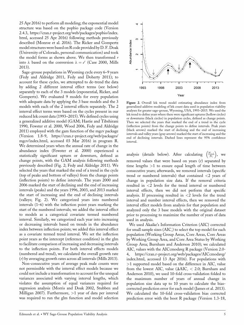
Table 1. Top models selected for population viability analyses of lek count data for greater sage-grouse populations, Wyoming, USA, 1993–2015, groupedbased onWorking Group Areas. Not all populations contained data from the full range of years investigated; we present the range and total number of years oflek count data analyzed. For each population, we present the finite rate of population growth (l) and 95% confidence intervals.

Population Years No. years Model l l 95% CI

Bates Hole–Shirley Basin 1997–2015 18 Ricker trend interval 0.993 0.986–<1.000Bighorn Basin 2003–2015 12 Exponential trend interval 1.061 0.823–1.368Northeast 1998–2015 17 Ricker trend interval 0.955 0.933–0.978South Central 1996–2015 19 Ricker trend interval 0.993 0.986–<1.000Southwest 1993–2015 22 Gompertz trend interval 0.704 0.560–0.883Upper Green River Basin 1997–2015 18 Gompertz trend interval 0.741 0.524–1.047Upper Snake River Basin 2003–2015 8 Exponential 1.078 0.853–1.360Wind River–Sweetwater River Basin 1993–2015 22 Gompertz trend interval 0.771 0.628–0.947

6 The Journal of Wildlife Management � 9999()

6 populations (Table S6, available online in SupportingInformation). Eleven of the Core Area Status populationswere declining, of which l differed from 1.0 for 7populations, and the remaining 5 populations were increas-ing (Table 4). The trend in l was similar between Core Areaand Non-Core Area populations for 7 of 8 Working GroupAreas (i.e., Core Area and Non-Core Area populations bothincreased or decreased); populations declined in 5 of those 7Working Group Areas (Fig. 6). The Core Area populationwas declining and the Non-Core Area population wasincreasing in the remainingWorking Group Area, theWindRiver-Sweetwater River Basin (Fig. 6). Similar to theWorking Group Area analysis, the Core Area and Non-CoreArea populations in the northwest (Bighorn Basin andUpper Snake River Basin) were increasing, and the mostseverely declining populations (l< 0.95) occurred in thesouthwest, central (except for Non-Core Areas in WindRiver-Sweetwater River Basin, which were increasing), andnortheast regions (Fig. 6). The Bates Hole-Shirley Basin

population declined at a slow rate (0.993) when analyzed as awhole (Table 1), but when analyzed separately by Core Areastatus, both the Core Area and Non-Core Areas weredeclining rapidly (0.828 and 0.731, respectively; Table 4),though the 95% confidence intervals for the l estimate of theNon-Core Area population overlapped 1.0, likely because ofsmall sample of leks counted per year. This discrepancy waslikely due to the Ricker trend interval being the top model forthe Working Group Area, whereas the Gompertz trendinterval and Gompertz were the top models for the CoreArea and Non-Core Areas. We provide further details belowwhy the Gompertz model results in lower l estimates, butbriefly it is due to the stronger density-dependent effect (thusmore extreme l estimates) with the Gompertz modelcompared to the Ricker model. Similar to the South CentralWorking Group Area results (0.993; Table 1), the SouthCentral Core Area population declined very slightly (0.995),but the Non-Core Area population was declining morerapidly (0.966; Table 4, Fig. 6).

Figure 3. Finite rate of population growth (l) of greater sage-grouse populations by Wyoming Game and Fish Department Working Group Area (labeled),Wyoming, USA, 1993–2015. We used lek count data to calculate population growth rate with population viability analyses.

Edmunds et al. � WY Sage-Grouse Population Viability Analysis 7

The average number of years of data for populations forwhich the exponential model was the top model was 7.650years (95% CI¼ 6.015–9.285), which was shorter than allother models, including the other 2 basic models (Gompertz:�x¼ 13.391, 95% CI¼ 11.562–15.221; Ricker: �x¼ 14.000,95% CI¼ 13.031–14.969). In all cases, the average numberof years for populations where the basic model was the topmodel were shorter than for populations where theequivalent model included the trend interval covariate(exponential trend interval: �x¼ 15.000, 95% CI¼ 13.654–16.346; Gompertz trend interval: �x¼ 18.684, 95% CI¼ 17.630–19.738; Ricker trend interval: �x¼ 17.111, 95%CI¼ 16.474–17.748). Within populations for which trendinterval models were the top selected, the average number ofyears analyzed was significantly shorter for exponential trendintervals compared to Gompertz trend interval populationsand nearly significantly shorter than Ricker trend intervalpopulations. We found that 12 years was the shortest lekcount data timeframe that resulted in l values that differedfrom 1.0 across all models. The Gompertz model resulted inthe lowest l estimates of the 3 model forms, ranging from0.207–0.731 for top selected models. The exponential modelresulted in the widest range in l estimates (0.753–1.509),whereas the Ricker model was the narrowest (0.948–0.984).The exponential model was the most common model form

for populations with<10 years of data and was the top modelfor 16 of such populations and the Gompertz model was thetop model for the remaining 2 populations.

DISCUSSION

We found that in general when we investigated Core Areastatus (Core Area vs. Non-Core Area) by Working GroupArea, the 2 populations tended to trend in the same directionand agreed with the overall trend of the Working GroupArea. However, at the finer scale where we analyzed CoreAreas separately within Working Group Areas, in mostinstances, Core Areas within the sameWorking Group Areatrended differently (5 out of 8 Working Groups). Forexample, the overall trend of the Bates Hole-Shirley BasinWorking Group Area was stable (l¼ 0.993), as was thelargest Core Area within its boundary, Natrona (l¼ 0.992).However, the remaining 3 Core Areas were all declining (lrange: 0.570–0.970) as was the Non-Core Area population(l¼ 0.970). In this Working Group Area, the Natrona CoreArea was driving the overall population trend and maskingthe population declines occurring in other Core Areas.Furthermore, the Bighorn Basin Working Group overalltrend was increasing slightly (l¼ 1.061) and the overall CoreArea population trend was increasing slightly as well(l¼ 1.059) when we investigated by Core Area status.

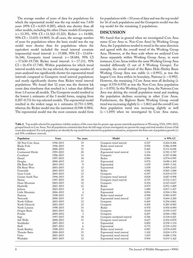
Table 2. Top models selected for population viability analyses of lek count data for greater sage-grouse statewide populations in Wyoming, USA, 1993–2015,grouped based on Core Areas. Not all populations contained data from the full range of years investigated; we present the range and total number of years of lekcount data analyzed. For each population, we identify the topmodel form selected for population estimation, and present the finite rate of population growth (l)and 95% confidence intervals.

Population Years No. years Model l l 95% CI

All Non-Core Areas 1996–2015 19 Gompertz trend interval 0.327 0.264–0.406Blacks Fork 1996–2015 19 Ricker trend interval 0.992 0.986–0.998Buffalo 2000–2015 15 Gompertz 0.465 0.311–0.696Continental Divide 1993–2015 20 Exponential trend interval 1.156 0.783–1.707Crowheart 1996–2015 14 Gompertz 0.384 0.307–0.480Daniel 1997–2015 18 Ricker 0.984 0.974–0.995Douglas 2000–2015 15 Exponential 0.972 0.690–1.369Elk Basin East 2003–2013 8 Exponential 1.039 0.805–1.341Elk Basin West 2003–2015 12 Exponential 1.038 0.409–2.633Fontenelle 2003–2015 12 Ricker 0.982 0.965–1.000Grass Creek 2003–2015 12 Gompertz 0.397 0.219–0.719Greater South Pass 1994–2015 21 Gompertz trend interval 0.828 0.687–0.998Hanna 1997–2015 18 Gompertz trend interval 0.735 0.531–1.017Heart Mountain 2003–2015 12 Gompertz 0.324 0.167–0.627Hyattville 2003–2015 12 Ricker 0.979 0.951–1.009Jackson 2003–2015 8 Exponential 1.080 0.817–1.427Little Mountain 2006–2015 4 Exponential 0.894 0.504–1.584Natrona 1998–2015 17 Ricker trend interval 0.990 0.983–0.997Newcastle 2000–2015 15 Exponential trend interval 1.225 0.664–2.260North Gillette 2003–2015 12 Gompertz 0.469 0.256–0.861North Glenrock 2003–2015 12 Gompertz 0.505 0.283–0.902North Laramie 1998–2015 15 Ricker 0.970 0.956–0.984Oregon Basin 2003–2015 12 Gompertz 0.610 0.359–1.037Powder 2009–2012 3 Gompertz 0.207 0.040–1.082Sage 1997–2015 18 Gompertz numbered interval 0.366 0.318–0.421Salt Wells 2000–2015 15 Gompertz trend interval 0.627 0.452–0.870Seedskadee 2007–2013 6 Exponential 0.802 0.558–1.154Shell 2007–2013 6 Exponential 0.753 0.539–1.052South Rawlins 1998–2015 15 Ricker trend interval 0.987 0.979–0.995Thunder Basin 2000–2015 15 Exponential trend interval 1.102 0.824–1.474Uinta 2003–2015 12 Exponential trend interval 1.035 0.688–1.556Washakie 2003–2015 12 Exponential trend interval 0.964 0.653–1.422

8 The Journal of Wildlife Management � 9999()

However, when we analyzed Core Area populations withinthe Bighorn Basin separately, 6 populations were declining.We also detected the reverse situation in the Northeast andSouthwest Working Groups. These Working Groups weredeclining overall and within both Core Area and Non-CoreArea populations when investigated by Core Area status.However, 2 Core Areas within the Northeast WorkingGroup and 3 Core Areas within the Southwest WorkingGroup were actually increasing. These examples highlightthe ability of relatively close populations to experiencedifferent population trends, likely because of localized factorsinfluencing trends at small scales.We developed an effective methodology to perform a PVA

at multiple spatial scales and varying lengths of time on aspecies with known population cycles that incorporateddensity-independent and density-dependent populationgrowth. We handled population cycles by incorporatinginterval covariates into the standard density-independentand density-dependent models and the top models includedinterval effects for half of the populations investigated (48%).

Populations with a longer number of years of data, and thus agreater potential to capture multiple 6–9-year cyclescommon in Wyoming (Fedy and Aldridge 2011), weremore likely to have the top model contain the trend intervalcovariate based on average number of years of data by modelstructure. The numbered interval covariate was not aseffective and was only the top model for 3 populations. Ingeneral, the large-scale populations (i.e., Working GroupAreas) tended to have more years of data compared to small-scale populations (i.e., Core Areas), which increased thelikelihood to include multiple cycles and thus likely increasedthe probability of the trend interval covariate to be includedin the top model. It also is possible that the difference in topmodel selection across scales was due to the potentialinfluences of those trends. At large spatial scales, broadpattern effects (e.g., climate) likely helped influencepopulation trends. At smaller scales, local factors (e.g., gasand oil development) likely influenced population trends.The trend interval covariate may have explained broad-scalepatterns such as climate, which is known to drive cyclic

Figure 4. Finite rate of population growth (l) of greater sage-grouse populations by Wyoming Core Population Areas (Core Areas), Wyoming, USA, 1993–2015. We used lek count data to calculate population growth rate with population viability analyses.

Edmunds et al. � WY Sage-Grouse Population Viability Analysis 9

patterns (Kausrud et al. 2008), better than local factors.Certain caveats should be clear when comparing l estimatesacross populations: 1) the model structure can affect themagnitude of l (e.g., at the broadest scale [Working GroupAreas] l estimates were most similar by model structure, notpopulation investigated; Table S7, available online inSupporting Information); 2) the number of years of datacan affect which model was the top selected; and 3) manypopulations did not contain data for the whole study period,so comparisons are most appropriate to populations withsimilar time periods assessed. However, we think that ourmodel selection methods (AICc followed by10-fold cross-validation) selected the best model structure that recoveredthe actual dynamics for each population as reflected in the

count data. Therefore, l estimates reflect population-specificdynamics occurring on the landscape and are not just theresult of a model structure that happened to be selected as thetop model. We think our methodologies are sound, andvariation in models selected (model structure) acrosspopulations represent true variation in biological processesthat are regulating individual populations.As mentioned above, model structure also affected the

magnitude of l values (Table S7). The Gompertz modelresulted in the lowest l values, whereas the exponential andRicker values were similar in range. This was true forcomparing top model results across populations and withinpopulation results. Pellet et al. (2006) used exponential,Gompertz, and Ricker models to model population growth

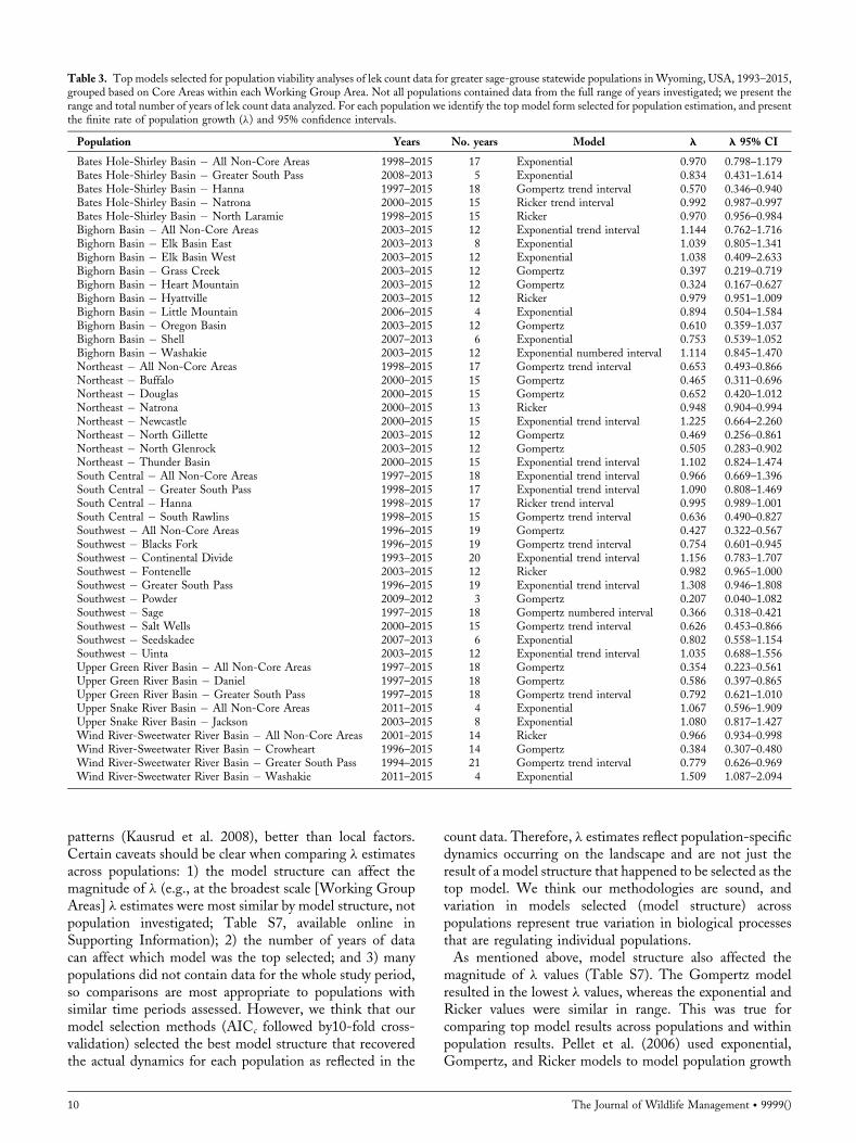
Table 3. Top models selected for population viability analyses of lek count data for greater sage-grouse statewide populations in Wyoming, USA, 1993–2015,grouped based on Core Areas within each Working Group Area. Not all populations contained data from the full range of years investigated; we present therange and total number of years of lek count data analyzed. For each population we identify the top model form selected for population estimation, and presentthe finite rate of population growth (l) and 95% confidence intervals.

Population Years No. years Model l l 95% CI

Bates Hole-Shirley Basin � All Non-Core Areas 1998–2015 17 Exponential 0.970 0.798–1.179Bates Hole-Shirley Basin � Greater South Pass 2008–2013 5 Exponential 0.834 0.431–1.614Bates Hole-Shirley Basin � Hanna 1997–2015 18 Gompertz trend interval 0.570 0.346–0.940Bates Hole-Shirley Basin � Natrona 2000–2015 15 Ricker trend interval 0.992 0.987–0.997Bates Hole-Shirley Basin � North Laramie 1998–2015 15 Ricker 0.970 0.956–0.984Bighorn Basin � All Non-Core Areas 2003–2015 12 Exponential trend interval 1.144 0.762–1.716Bighorn Basin � Elk Basin East 2003–2013 8 Exponential 1.039 0.805–1.341Bighorn Basin � Elk Basin West 2003–2015 12 Exponential 1.038 0.409–2.633Bighorn Basin � Grass Creek 2003–2015 12 Gompertz 0.397 0.219–0.719Bighorn Basin � Heart Mountain 2003–2015 12 Gompertz 0.324 0.167–0.627Bighorn Basin � Hyattville 2003–2015 12 Ricker 0.979 0.951–1.009Bighorn Basin � Little Mountain 2006–2015 4 Exponential 0.894 0.504–1.584Bighorn Basin � Oregon Basin 2003–2015 12 Gompertz 0.610 0.359–1.037Bighorn Basin � Shell 2007–2013 6 Exponential 0.753 0.539–1.052Bighorn Basin � Washakie 2003–2015 12 Exponential numbered interval 1.114 0.845–1.470Northeast � All Non-Core Areas 1998–2015 17 Gompertz trend interval 0.653 0.493–0.866Northeast � Buffalo 2000–2015 15 Gompertz 0.465 0.311–0.696Northeast � Douglas 2000–2015 15 Gompertz 0.652 0.420–1.012Northeast � Natrona 2000–2015 13 Ricker 0.948 0.904–0.994Northeast � Newcastle 2000–2015 15 Exponential trend interval 1.225 0.664–2.260Northeast � North Gillette 2003–2015 12 Gompertz 0.469 0.256–0.861Northeast � North Glenrock 2003–2015 12 Gompertz 0.505 0.283–0.902Northeast � Thunder Basin 2000–2015 15 Exponential trend interval 1.102 0.824–1.474South Central � All Non-Core Areas 1997–2015 18 Exponential trend interval 0.966 0.669–1.396South Central � Greater South Pass 1998–2015 17 Exponential trend interval 1.090 0.808–1.469South Central � Hanna 1998–2015 17 Ricker trend interval 0.995 0.989–1.001South Central � South Rawlins 1998–2015 15 Gompertz trend interval 0.636 0.490–0.827Southwest � All Non-Core Areas 1996–2015 19 Gompertz 0.427 0.322–0.567Southwest � Blacks Fork 1996–2015 19 Gompertz trend interval 0.754 0.601–0.945Southwest � Continental Divide 1993–2015 20 Exponential trend interval 1.156 0.783–1.707Southwest � Fontenelle 2003–2015 12 Ricker 0.982 0.965–1.000Southwest � Greater South Pass 1996–2015 19 Exponential trend interval 1.308 0.946–1.808Southwest � Powder 2009–2012 3 Gompertz 0.207 0.040–1.082Southwest � Sage 1997–2015 18 Gompertz numbered interval 0.366 0.318–0.421Southwest � Salt Wells 2000–2015 15 Gompertz trend interval 0.626 0.453–0.866Southwest � Seedskadee 2007–2013 6 Exponential 0.802 0.558–1.154Southwest � Uinta 2003–2015 12 Exponential trend interval 1.035 0.688–1.556Upper Green River Basin � All Non-Core Areas 1997–2015 18 Gompertz 0.354 0.223–0.561Upper Green River Basin � Daniel 1997–2015 18 Gompertz 0.586 0.397–0.865Upper Green River Basin � Greater South Pass 1997–2015 18 Gompertz trend interval 0.792 0.621–1.010Upper Snake River Basin � All Non-Core Areas 2011–2015 4 Exponential 1.067 0.596–1.909Upper Snake River Basin � Jackson 2003–2015 8 Exponential 1.080 0.817–1.427Wind River-Sweetwater River Basin � All Non-Core Areas 2001–2015 14 Ricker 0.966 0.934–0.998Wind River-Sweetwater River Basin � Crowheart 1996–2015 14 Gompertz 0.384 0.307–0.480Wind River-Sweetwater River Basin � Greater South Pass 1994–2015 21 Gompertz trend interval 0.779 0.626–0.969Wind River-Sweetwater River Basin � Washakie 2011–2015 4 Exponential 1.509 1.087–2.094

10 The Journal of Wildlife Management � 9999()

Figure 5. Finite rate of population growth (l) of greater sage-grouse populations by Wyoming Core Population Areas (Core Areas) grouped by WyomingGame and Fish Department Working Group Areas (labeled), Wyoming, USA, 1993–2015. We used lek count data to calculate population growth rate withpopulation viability analyses.

Table 4. Top models selected for population viability analyses of lek count data for greater sage-grouse statewide populations in Wyoming, USA, 1993–2015,grouped based onCore Areas status (Core Area vs. Non-CoreArea) within eachWorkingGroupArea. Not all populations contained data from the full range ofyears investigated; we present the range and total number of years of lek count data analyzed. For each population we identify the top model form selected forpopulation estimation, and present the finite rate of population growth (l) and 95% confidence intervals.

Population Years No. years Model l l 95% CI

Bates Hole-Shirley Basin � Core Areas 1997–2015 18 Gompertz trend interval 0.828 0.687–0.997Bates Hole-Shirley Basin � Non-Core Areas 1998–2015 17 Gompertz 0.731 0.504–1.059Bighorn Basin � Core Areas 2003–2015 12 Exponential trend interval 1.059 0.814–1.378Bighorn Basin � Non-Core Areas 2003–2015 12 Exponential trend interval 1.144 0.762–1.716Northeast � Core Areas 1998–2015 17 Ricker 0.953 0.929–0.978Northeast � Non-Core Areas 1998–2015 17 Gompertz trend interval 0.653 0.493–0.866South Central � Core Areas 1998–2015 17 Ricker trend interval 0.995 0.988–1.002South Central � Non-Core Areas 1997–2015 18 Exponential trend interval 0.966 0.669–1.396Southwest � Core Areas 1993–2015 22 Gompertz trend interval 0.708 0.563–0.890Southwest � Non-Core Areas 1996–2015 19 Gompertz 0.427 0.322–0.567Upper Green River Basin � Core Areas 1997–2015 18 Gompertz trend interval 0.787 0.576–1.074Upper Green River Basin � Non-Core Areas 1997–2015 18 Gompertz 0.354 0.223–0.561Upper Snake River Basin � Core Areas 2003–2015 8 Exponential 1.080 0.817–1.427Upper Snake River Basin � Non-Core Areas 2011–2015 4 Exponential 1.067 0.596–1.909Wind River-Sweetwater River Basin � Core Areas 1993–2015 22 Gompertz trend interval 0.770 0.624–0.950Wind River-Sweetwater River Basin � Non-Core Areas 2001–2015 14 Exponential trend interval 1.340 0.667–2.692

Edmunds et al. � WY Sage-Grouse Population Viability Analysis 11

in European tree frogs (Hyla arborea) and growth rates werelowest for the Gompertz model as well; the growth ratescalculated with the exponential and Ricker models weremore similar with the exponential growth rate being higher.All growth rates of tree frogs showed declining populationtrends. However, Colchero et al. (2009) modeled populationgrowth of an isolated desert bighorn sheep (Ovis canadensis)population with the same 3 models and reported that theGompertz model resulted in the highest growth rate by far,whereas the exponential and Ricker models resulted in moresimilar growth rates once again, with the exponential growthrate being the lowest. In this case study on bighorn sheep,populations had increasing growth rates. It appears that theRicker and exponential models tend to attenuate growthestimates toward stable growth, whereas the Gompertzmodel tends to estimate more extreme population growthrates. This is likely due to the stronger density-dependenteffect at small population sizes caused by the way in whichthe model is implemented. There is a constant linear decrease

in r as the natural logarithm of population size increases;therefore, the density-dependent effect becomes lesspronounced as population sizes increase.We are not able to make direct comparisons between our

population trends and previous studies because we useddifferent population delineations; however, we can formulategeneral comparisons. The Northeast Working Group Areaoverlapped most of the Powder River Basin populationanalyzed by Garton et al. (2011, 2015), who reported a 0.3%annual decline from 1965–2013. Our l estimate of 0.955 forthe Northeast population corresponded to a much largerannual decline of 4.5% from 1998–2015. The Powder RiverBasin population included leks in southeastMontana and therange of years analyzed differed between the studies;however, both studies indicate that this population hasdeclined over the past several decades. Based on the weightedaverage of Working Group Area l estimates, we indicated a9.9% statewide annual decline. Three additional studiesinvestigated Wyoming statewide trends based on lek count

Figure 6. Finite rate of population growth (l) of greater sage-grouse populations by Wyoming Core Population Area status (Core Area vs. Non-Core Area)grouped by Wyoming Game and Fish Department Working Group Areas (labeled), Wyoming, USA, 1993–2015. We used lek count data to calculatepopulation growth rate with population viability analyses.

12 The Journal of Wildlife Management � 9999()

data. Green et al. (2017) documented annual statewidedeclines of 2.5% during 1984–2008, Monroe et al. (2017)reported annual statewide declines of 6.0% during 2004–2014, and Fedy and Aldridge (2011) reported an overallstatewide population decline of 54% during 1968–2006,which averaged a 1.4% annual decline. All of these studiesused different leks, time periods, and models in analyses,which partly explains the varying population growthestimates; however, taken together it is clear statewidesage-grouse populations in Wyoming have declined over thepast several decades.Walker et al. (2007) also investigated sage-grouse

population trends in the Powder River Basin during2001–2005. Leks were divided into those located withincoal bed natural gas fields and those located outside gas fields.Again, comparisons are not direct because we investigated alonger time frame and we did not divide leks into groupsbased on gas fields. However, our 4.5% estimated annualdecline closely resembled the non-gas field annual popula-tion decline of 3.0%; the gas field population declined 35%per year (Walker et al. 2007). Perhaps a better evaluationwould be to compare non-gas field populations to Core Areapopulations within the Northeast Working Group becauseCore Area boundaries were developed to represent suitablehabitat, from which disturbed lands were excluded (State ofWyoming 2015). Core Area populations within theNortheast Working Group declined similarly to the wholeWorking Group Area population at an annual decline of4.7%, which again was similar to non-gas field populationsreported by Walker et al. (2007).Annual population trends also were estimated for gas field

and non-gas field populations in western Wyoming withinthe Upper Green River Basin Working Group Area during1998–2004 (Holloran 2005). Holloran (2005) documented a21.3% annual decline for the gas field population and a 13.4%annual decline for the non-gas field population. Weestimated a more drastic annual decline of 25.9% for theWorking Group Area population, albeit over a longer period(1997–2015) and the 95% confidence intervals overlapped1.0 slightly. We also estimated a 21.3% annual decline forCore Area populations within the Upper Green River Basin(presumably non-gas field populations) and a 64.6% annualdecline for the Non-Core Area population; in this case the lestimate comparisons do not match well. These populationdeclines occurred during a rise in active gas and oil wells (by4.4 times) located within the Upper Green River BasinWorking Group Area over the same time period (WyomingOil and Gas Conservation Coalition, http://wogcc.state.wy.us, accessed 15 Oct 2015). Notably, the Core Areas and theirassociated protections were not developed until 2008 (Stateof Wyoming 2008), and our study period went back to 1997for this population.The general trend in l was similar between Core Area and

Non-Core Area populations for 7 out of 8 Working GroupAreas (Fig. 6). Core Area and Non-Core Area populationswere both increasing in the Bighorn Basin (l¼ 1.059and 1.144, respectively). For the Upper Green RiverBasin, Southwest, Bates Hole-Shirley Basin, and Northeast

Working Group Areas, both Core Area and Non-Core Areapopulations were declining, with the Northeast Core Areapopulation having the highest l value of 0.955. The CoreArea population in the South Central Working Group wasstable (l¼ 0.995), while the Non-Core Area population wasdeclining more substantially (l¼ 0.966); however, the 95%confidence intervals overlapped 1.0 for both populations.The one case where the 2 population trends diverged was intheWind River-Sweetwater River BasinWorking Group, inwhich the Core Area population was declining (l¼ 0.770)and the Non-Core Area population was increasing(l¼ 1.340). Although it is interesting to compare CoreArea versus Non-Core Area trends, we did not intend thisanalysis to be an evaluation of the Core Area strategy asevidenced by our choice to investigate trends dating back to1993. Also, by the nature of how Core Areas wereestablished, in which approximately 83% of the sage-grousepopulation was encompassed in approximately 24% of thesurface areas of the state (State of Wyoming 2015), theycontained a larger sample size of leks counted compared toNon-Core Areas in all but the Northeast Working GroupArea. The number of leks counted were still comparablebetween Core and Non-Core Areas in all but the BatesHole-Shirley Basin, Bighorn Basin, and Upper Snake RiverBasin Working Groups, which contained <10 leks annuallyin Non-Core Areas. The Core Area delineations were aconvenient scale at which to investigate population trends ata finer resolution than the Working Group Areas andmanagement decisions are applied at both scales. Movingforward, using Core Areas will be an important approach tomonitor sage-grouse population trends because Core Areapopulations are managed in a much more conservativemanner than Non-Core Area populations to ensure theprotection of this species in Wyoming (State of Wyoming2015). Furthermore, it is concerning for sage-grousemanagement that the Core Area delineations were selectedfor protections because they were presumably the best andmost stable populations in Wyoming even prior to theincreased protections in 2008, and yet 77% of the Core Areapopulations were declining and 4 out of 7 of the remainingpopulations were merely stable.When managing a species of concern, we should evaluate

the possibility that adjacent populations could be experienc-ing different population trends to determine what localfactors are influencing small-scale population trends and notassume that large-scale trends entirely account for what isoccurring across the landscape. For example, a localpopulation affected by a gas and oil field may be decliningannually, but the larger-scale trend may mask the declinebecause the larger population, which is located in a regionexperiencing increased spring precipitation and thus higherchick survival, is increasing. To assist with determiningpopulation trends and influences on those trends acrossmultiple spatial scales and how small-scale trends may beaffecting large-scale populations, clustering leks based onbiologically relevant landscape features and climatic con-ditions in a hierarchical, nested approach could be used tobetter define population boundaries.

Edmunds et al. � WY Sage-Grouse Population Viability Analysis 13

MANAGEMENT IMPLICATIONS

Core Area and Working Group Area population delin-eations are relevant to Wyoming sage-grouse managementbecause both are important in helping WGFD manage thisspecies. Our approach of monitoring populations at differentspatial scales using these boundaries will allow managers tofocus efforts on small-scale populations (Core Areas orportions of Core Areas located within specific WorkingGroup Areas) that are doing the poorest and influencing thelarger-scale population trends downward. Focusing man-agement efforts toward smaller-scale populations should be amore efficient use of time and resources to better assist withspecies protections and also could support further inves-tigations into factors influencing population change.Conversely, determining the fine-scale populations thatare stable or increasing through this analysis could assistmanagers with identifying which management strategieshave been most effective. Those strategies could then beapplied more broadly in other populations that are declining,where appropriate.

ACKNOWLEDGMENTS

Any use of trade, firm, or product names is for descriptivepurposes only and does not imply endorsement by the U.S.Government. We thank T. J. Christiansen for allowingaccess to lek count data and providing helpful revisions toearlier drafts that improved our manuscript. We areincredibly grateful to B. R. Noon for assistance with modelstructures for the PVA and with statistical consultation. Wethank B. S. Cade and B. C. Fedy for statistical consultationregarding model selection. We also thank D. F. Doak forsharing program R code on which we based the Ricker andGompertz model structures. We are indebted to T. E.Fulbright, P. R. Krausman, and 2 anonymous reviewers formaking suggestions that improved the final manuscript.Finally, we thank J. A. Heinrichs and A. W. Green for theirhelpful input during analysis. The United States GeologicalSurvey and theWyoming Landscape Conservation Initiativeprovided support for this work.

LITERATURE CITEDAldridge, C. L., and R. M. Brigham. 2003. Distribution, abundance, andstatus of the greater sage-grouse, Centrocercus urophasianus, in Canada.Canadian Field-Naturalist 117:25–34.

Beck, J. L., and D. L. Mitchell. 2000. Influences of livestock grazing on sagegrouse habitat. Wildlife Society Bulletin:993–1002.

Beetle, A. A., and K. L. Johnson. 1982. Sagebrush ofWyoming. Report 779.Agricultural Experiment Station, University ofWyoming, Laramie, USA.

Beever, E. A., and C. L. Aldridge. 2011. Influences of free-roaming equidson sagebrush ecosystems, with a focus on greater sage-grouse. Studies inAvian Biology 38:273–290.

Bissonette, J. A. 1997. Scale-sensitive ecological properties: historicalcontext, current meaning. Pages 3–31 in J. A. Bissonette, editor. Wildlifeand landscape ecology: effects of pattern and scale. Springer-Verlag, NewYork, New York, USA.

Bissonette, J. A. 2017. Avoiding the scale sampling problem: a consilientsolution. Journal of Wildlife Management 81:192–205.

Blomberg, E. J., J. S. Sedinger, D. V. Nonne, and M. T. Atamian. 2013.Annual male lek attendance influences count-based population indices ofgreater sage-grouse. Journal of Wildlife Management 77:1583–1592.

Branton, M., and J. S. Richardson. 2011. Assessing the value of theumbrella-species concept for conservation planning with meta-analysis.Conservation Biology 25:9–20.

Braun, C. E. 1998. Sage grouse declines in western North America: what arethe problems? Proceedings of the Western Association of State Fish andWildlife Agencies 78:139–156.

Braun, C. E., O. O. Oedekoven, and C. L. Aldridge. 2002. Oil and gasdevelopment in western North America: effects on sagebrush steppeavifauna with particular emphasis on sage-grouse. Transactions of theNorth AmericanWildlife and Natural Resources Conference 67:337–349.

Burnham, K. P., and D. R. Anderson. 2010. Model selection andmultimodel inference: a practical information-theoretic approach. Secondedition. Springer-Verlag, New York, New York, USA.

Cagney, J., E. Bainter, B. Budd, T. J. Christiansen, V. Herren, M. J.Holloran, B. Rashford, M. Smith, and J. Williams. 2010. Grazinginfluence, objective development, and management in Wyoming Greatersage-grouse habitat: with emphasis on besting and early brood rearing.University of Wyoming Extension, Laramie, USA.

Case, T. J. 2000. An illustrated guide to theoretical ecology. OxfordUniversity Press, New York, New York, USA.

Christiansen, T. J. 2012. Sage-grouse (Centrocercus urophasianus). Pages 12-1–12-55 in S. A. Tessman and J. R. Bohne, editors. Handbook ofbiological techniques. Third edition. Wyoming Game and FishDepartment, Cheyenne, USA.

Christiansen, T. J., and N. Whitford. 2015. Wyoming greater sage-grousecurrent range 2015. Wyoming Game and Fish Department. https://wgfd.wyo.gov/Habitat/Sage-Grouse-Management. Accessed 7 Aug 2015.

Colchero, F., R. A. Medellin, J. S. Clark, R. Lee, and G. G. Katul. 2009.Predicting population survival under future climate change: densitydependence, drought and extraction in an insular bighorn sheep. Journal ofAnimal Ecology 78:666–673.

Collins, B. T. 1990. Using rerandomizing tests in route-regression analysisof avian population trends. Pages 63–70 in J. R. Sauer and S. Droege,editors. Survey designs and statistical methods for the estimation of avianpopulation trends. U.S. Fish andWildlife Service Biological Report 90(1),Laurel, Maryland, USA.

Connelly, J. W., and C. E. Braun. 1997. Long-term changes in sage grouseCentrocercus urophasianus populations in western North America.Wildlife Biology 3:229–234.

Connelly, J. W., C. A. Hagen, and M. A. Schroeder. 2011a. Characteristicsand dynamics of greater sage-grouse populations. Studies in Avian Biology38:53–67.

Connelly, J. W., S. T. Knick, M. A. Schroeder, and S. J. Stiver. 2004.Conservation assessment of greater sage-grouse and sagebrush habitats.Western Association of Fish andWildlife Agencies Cheyenne,Wyoming,USA.

Connelly, J. W., K. P. Reese, R. A. Fischer, and W. L. Wakkinen. 2000.Response of a sage grouse breeding population to fire in southeasternIdaho. Wildlife Society Bulletin 28:90–96.

Connelly, J. W., E. T. Rinkes, and C. E. Braun. 2011b. Characteristics ofgreater sage-grouse habitats. Studies in Avian Biology 38:69–83.

Copeland, H. E., A. Pocewicz, D. E. Naugle, T. Griffiths, D. Keinath, J.Evans, and J. Platt. 2013. Measuring the effectiveness of conservation: anovel framework to quantify the benefits of sage-grouse conservationpolicy and easements in Wyoming. PLoS ONE 8:e67261.

Crawford, J. A., R. A. Olson, N. E. West, J. C. Mosley, M. A. Schroeder,T. D.Whitson, R. F. Miller, M. A. Gregg, and C. S. Boyd. 2004. Ecologyandmanagement of sage-grouse and sage-grouse habitat. Journal of RangeManagement 57:2–19.

Dahlgren, D. K., M. R. Guttery, T. A. Messmer, D. Caudill, R. DwayneElmore, R. Chi, and D. N. Koons. 2016. Evaluating vital ratecontributions to greater sage-grouse population dynamics to informconservation. Ecosphere 7:e01249.

Dennis, B., P. L. Munholland, and J. M. Scott. 1991. Estimation of growthand extinction parameters for endangered species. Ecological Monographs61:115–143.

Dennis, B., and M. L. Taper. 1994. Density dependence in time seriesobservations of natural populations: estimation and testing. EcologicalMonographs 64:205–224.

DeSante, D. F., M. P. Nott, and D. R. O’Grady. 2001. Identifying theproximate demographic cause (s) of population change by modelling

14 The Journal of Wildlife Management � 9999()

spatial variation in productivity, survivorship, and population trends.Ardea 89:185–208.

Doherty, K. E., J. D. Tack, J. S. Evans, and D. E. Naugle. 2010. Mappingbreeding densities of greater sage-grouse: a tool for range-wideconservation planning. Completion report to the Bureau of LandManagement for Interagency Agreement # L10PG00911, Washington,D.C., USA.

Fedy, B. C., and C. L. Aldridge. 2011. The importance of within-yearrepeated counts and the influence of scale on long-term monitoring ofsage-grouse. Journal of Wildlife Management 75:1022–1033.

Fedy, B. C., and K. E. Doherty. 2011. Population cycles are highly correlatedover long time series and large spatial scales in two unrelated species:greater sage-grouse and cottontail rabbits. Oecologia 165:915–924.

Fewster, R. M., S. T. Buckland, G. M. Siriwardena, S. R. Baillie, and J. D.Wilson. 2000. Analysis of population trends for farmland birds usinggeneralized additive models. Ecology 81:1970–1984.

Fieberg, J., and S. P. Ellner. 2000. When is it meaningful to estimate anextinction probability? Ecology 81:2040–2047.

Fuhlendorf, S. D., A. J. W. Woodward, D. M. Leslie, and J. S. Shackford.2002. Multi-scale effects of habitat loss and fragmentation on lesserprairie-chicken populations of the US Southern Great Plains. LandscapeEcology 17:617–628.

Garton, E. O., J. W. Connelly, J. S. Horne, C. A. Hagen, A. Moser, andM. A. Schroeder. 2011. Greater sage-grouse population dynamics andprobability of persistence. Studies in Avian Biology 38:293–382.

Garton, E. O., A. G. Wells, J. A. Baumgardt, and J. W. Connelly. 2015.Greater sage-grouse population dynamics and probability of persistence.Pew Charitable Trusts, Philadelphia, Pennsylvania, USA. http://www.pewtrusts.org/~/media/assets/2015/04/garton-et-al-2015-greater-sagegrouse-population-dynamics-and-persistence-31815.pdf.

Geissler, P. H., and B. R. Noon. 1981. Estimates of avian population trendsfrom the North American Breeding Bird Survey. Studies in Avian Biology6:42–51.

Gerber, L. R., D. P. Demaster, and P. M. Kareiva. 1999. Gray whales andthe value of monitoring data in implementing the US Endangered SpeciesAct. Conservation Biology 13:1215–1219.

Green, A. W., C. L. Aldridge, and M. S. O’Donnell. 2017. Investigatingimpacts of oil and gas development on greater sage-grouse. Journal ofWildlife Management 81:46–57.

Hanser, S. E., and S. T. Knick. 2011. Greater sage-grouse as an umbrellaspecies for shrubland passerine birds. Studies in Avian Biology38:473–487.

Hastie, T. J., and R. J. Tibshirani. 1990. Generalized additive models.Volume 43. Chapman & Hall, New York, New York, USA.

Hayes, G. F., and K. D. Holl. 2003. Cattle grazing impacts on annual forbsand vegetation composition of mesic grasslands in California. Conserva-tion Biology 17:1694–1702.

Holloran, M. J. 2005. Greater sage-grouse (Centrocercus urophasianus)population response to natural gas field development in westernWyoming. Dissertation, University of Wyoming, Laramie, USA.

Holmes, E. E. 2001. Estimating risks in declining populations with poordata. Proceedings of the National Academy of Sciences 98:5072–5077.

Jacobson, A. R., A. Provenzale, A. von Hardenberg, B. Bassano, and M.Festa-Bianchet. 2004. Climate forcing and density dependence in amountain ungulate population. Ecology 85:1598–1610.

James, G., D. Witten, T. Hastie, and R. Tibshirani. 2013. An introduction tostatistical learningwith applications inR.Springer,NewYork,NewYork,USA.

Kausrud, K. L., A. Mysterud, H. Steen, J. O. Vik, E.Østbye, B. Cazelles, E.Framstad, A. M. Eikeset, I. Mysterud, and T. Solhøy. 2008. Linkingclimate change to lemming cycles. Nature 456:93–97.

Knick, S. T., D. S. Dobkin, J. T. Rotenberry, M. A. Schroeder, W. M.Vander Haegen, and C. van Ripper III. 2003. Teetering on the edge or toolate? Conervation and research issues for avifauna of sagebrush habitats.Condor 105:611–634.

Ludwig, D. 1999. Is it meaningful to estimate a probability of extinction?Ecology 80:298–310.

Lyon, A. G., and S. H. Anderson. 2003. Potential gas development impactson sage grouse nest initiation and movement. Wildlife Society Bulletin31:486–491.

Mills, L. S. 2013. Conservation of wildlife populations: demography,genetics, and management. Second edition. John Wiley & Sons,Chichester, West Sussex, United Kingdom.

Monroe, A. P., C. L. Aldridge, T. J. Assal, K. E. Veblen, D. A. Pyke, andM. L. Casazza. 2017. Patterns in greater sage-grouse population dynamicscorrespond with public grazing records at broad scales. EcologicalApplications 27:1096–1107.

Monroe, A. P., D. R. Edmunds, and C. L. Aldridge. 2016. Effects of lekcount protocols on greater sage-grouse population trend estimates. Journalof Wildlife Management 80:667–678.

Morris, W., D. Doak, M. Groom, P. Kareiva, J. Fieberg, L. Gerber, P.Murphy, and D. Thomson. 1999. A practical handbook for populationviability analysis. The Nature Conservancy, Arlington, Virginia, USA.

Morris, W. F., and D. F. Doak. 2002. Quantitative conservation biology:theory and practice of population viability analysis. Sinauer, Sunderland,Massachusetts, USA.

Nicholls, A., P. Viljoen, M. Knight, and A. Van Jaarsveld. 1996. Evaluatingpopulation persistence of censused and unmanaged herbivore populationsfrom the Kruger National Park, South Africa. Biological Conservation76:57–67.

Noss, R. F., E.T.LaRoe III, and J.M. Scott. 1995. Endangered ecosystemsofthe United States: a preliminary assessment of loss and degradation. USDINational Biological Service Biological Report 28,Washington,D.C., USA.

Pellet, J., B. R. Schmidt, F. Fivaz, N. Perrin, and K. Grossenbacher. 2006.Density, climate and varying returnpoints: an analysis of long-termpopulationfluctuations in the threatened European tree frog. Oecologia 149:65–71.

Reed, J. M., L. S. Mills, J. B. Dunning, E. S. Menges, K. S. McKelvey, R.Frye, S. R. Beissinger, M. C. Anstett, and P. Miller. 2002. Emergingissues in population viability analysis. Conservation Biology 16:7–19.

Rich, T. 1985. Sage grouse population fluctuations: evidence for a 10-yearcycle. U.S. Department of Interior, Bureau of Land Management, IdahoState Office, Technical Bulletin 85-1, Boise, Idaho, USA.

Ricker,W. E. 1954. Stock and recruitment. Journal of the Fisheries Board ofCanada 11:559–623.

Rowland, M. M., M. J. Wisdom, L. H. Suring, and C. W. Meinke. 2006.Greater sage-grouse as an umbrella species for sagebrush-associatedvertebrates. Biological Conservation 129:323–335.

Sadoul, N. 1997. The Importance of spatial scales in long-term monitoring ofcolonial Charadriiformes in Southern France.ColonialWaterbirds 20:330–338.

Schroeder, M. A., C. L. Aldridge, A. D. Apa, J. R. Bohne, C. E. Braun,S. D. Bunnell, J. W. Connelly, P. A. Deibert, S. C. Gardner, M. A.Hilliard, G. D. Kobriger, S. M. McAdam, C. W. McCarthy, J. J.McCarthy, D. L. Mitchell, E. V. Rickerson, and S. J. Stiver. 2004.Distribution of sage-grouse in North America. Condor 106:363–376.

Schultz, C. B., and P. C. Hammond. 2003. Using population viabilityanalysis to develop recovery criteria for endangered insects: case study ofthe Fender’s blue butterfly. Conservation Biology 17:1372–1385.

State ofWyoming. 2008. Greater sage-grouse core area protection. Office ofthe Governor, Executive Order 2008-2, Cheyenne, Wyoming, USA.

State ofWyoming. 2015. Greater sage-grouse core area protection. Office ofthe Governor, Executive Order 2015-4, Cheyenne, Wyoming, USA.

Stubben, C. J., and B. G. Milligan. 2007. Estimating and analyzingdemographic models using the popbio package in R. Journal of StatisticalSoftware 22:1–23.

U.S. Fish andWildlife Service [USFWS]. 2010. Endangered and threatenedwildlife and plants; 12-month findings for petitions to list the greater sage-grouse (Centrocercus urophasianus) as threatend or endangered; proposedrule. Federal Register 75:13910–14014.

U.S. Fish andWildlife Service [USFWS]. 2015. Endangered and threatnedwildlife and plants; 12-month finding on a petition to list greater sage-grouse (Centrocercus urophasianus) as an endangered or threatened species.Federal Register 80:59858–59942.

Walker, B. L., D. E. Naugle, and K. E. Doherty. 2007. Greater sage-grousepopulation response to energy development and habitat loss. Journal ofWildlife Management 71:2644–2654.

Wallace, B. P., A. D. DiMatteo, B. J. Hurley, E. M. Finkbeiner, A. B.Bolten, M. Y. Chaloupka, B. J. Hutchinson, F. A. Abreu-Grobois, D.Amorocho, K. A. Bjorndal, J. Bourjea, B. W. Bowen, R. B. Due~nas, P.Casale, B. C. Choudhury, A. Costa, P. H. Dutton, A. Fallabrino, A.Girard, M. Girondot, M. H. Godfrey, M. Hamann, M. L�opez-Mendilaharsu, M. A. Marcovaldi, J. A. Mortimer, J. A. Musick, R.Nel, N. J. Pilcher, J. A. Seminoff, S. Troëng, B. Witherington, and R. B.Mast. 2010. Regional management units for marine turtles: a novelframework for prioritizing conservation and research across multiplescales. PLoS ONE 5:e15465.

Edmunds et al. � WY Sage-Grouse Population Viability Analysis 15

Walsh, D. P., G. C. White, T. E. Remington, and D. C. Bowden. 2004.Evaluation of the lek-count index for greater sage-grouse.Wildlife SocietyBulletin 32:56–68.

Western Regional Climate Center [WRCC]. 2016. Climate of Wyoming.http://www.wrcc.dri.edu/narratives/WYOMING.htm. Accessed 13 Aug2015.

Wilcox, C., and H. Possingham. 2002. Do life history traits affect theaccuracy of diffusion approximations for mean time to extinction?Ecological Applications 12:1163–1179.

Wisdom, M. J., M. M. Rowland, B. C. Wales, M. A. Hemstrom, W. J.Hann, M. G. Raphael, R. S. Holthausen, R. A. Gravenmier, and T. D.Rich. 2002. Modeled effects of sagebrush-steppe restoration on greatersage-grouse in the Interior Columbia Basin, USA. Conservation Biology16:1223–1231.

Wood, S. N. 2006. Generalized additive models: an introduction with R.Chapman & Hall, New York, New York, USA.

Wyoming Game and Fish Department [WGFD]. 2003. Wyoming greatersage-grouse conservation plan. Wyoming Game and Fish Department,Cheyenne, USA.

Associate Editor: Timothy Fulbright.

SUPPORTING INFORMATION

Additional supporting information may be found in theonline version of this article at the publisher’s website.

16 The Journal of Wildlife Management � 9999()