GRD 2.0: An extended SPSS extension command for generating ... · ¦2015 Vol. 11 no. 3 GRD 2.0: An...

¦ 2015 Vol. 11 no. 3

GRD 2.0: An extended SPSS extension command forgenerating random data

Bradley Hardinga and Denis Cousineaua,�

aÉcole de psychologie, Université d’Ottawa

Abstract The GRD extension command for SPSS (Harding & Cousineau, 2014) has been used in a variety of applicationssince its inception. Ranging from a teaching tool to demonstrate statistical analyses, to an inferential tool used to findcritical values instead of looking into a z-table, GRD has been very well received. However, some users have requestedother data generation components that would make GRD a more complete extension command: the possibility to addcontaminants to the generated dataset as well as the ability to generate correlated variables. Another component weadded is a graphical user interface (or GUI) that makes GRD accessible through the drop-down menus in the SPSS DataEditor window. This GUI allows users to generate a simple dataset by entering parameters in dedicated fields rather thanwriting out the full script. Finally, we devised a small series of exercises to help users get acquainted with the new sub-commands and GUI.

Keywords GRD, Graphical User Interface, Contaminants, Correlation, Sampling

� [email protected]

Introduction

Statistics are often seen as the black sheep of an under-graduate degree in Psychology with students sometimesdeveloping anxiety towards the subject matter. For thisreason, teachers often give students a series of datasetsto practice concepts learnt in class on their own time.However, once the available datasets have been exhausted,novelty is thwarted as the students already know the an-swers. It is for this reason that we have developed an ex-tension command for SPSS that generates random data,GRD (standing for Generator of Random Data; Harding andCousineau (2014)). This extension command uses simplesub-commands and parameters written directly in SPSSSyntax and generates a completely different dataset everytime the command is run. We have used this commandextensively as a teaching tool in an introductory under-graduate statistics class, eliciting a strong positive recep-tion. Some students even used the command to generatedata similar to their homework’s dataset to infer whetheror not their answer could be correct. However, there aresome limitations to the command as pointed out by sev-eral students and other users. GRD has no option to simu-late multimodality and outliers short of inserting/modify-ing the data manually. In addition, GRD could not generatevariables that are correlated with one another. We thereforeadded these options in this new version of GRD.

Another aspect on which we have received many com-

ments on is the fact that the syntax language of SPSS canhave a steep learning curve. In addition to learning a largeamount of statistical concepts, learning the syntax of it allcan be overwhelming for students - especially if all that isrequired is a simple generated dataset. Therefore we haveadded a graphical user interface (GUI hereafter) that makesthe command more accessible to users that are not wellversed in SPSS syntax. While syntax allows one to save thescript and gives more control to the user, a GUI allows fora quick generation of a simple dataset. This new GUI is ac-cessible through the drop-down menus.

The following tutorial is organized in three main sec-tions. The first section shows how to use the two newoptions using SPSS syntax, as introduced in (Harding &Cousineau, 2014). The second section is an overview ofthe GUI for GRD, describing the input fields. The thirdsection shows three examples of classroom-ready exercisespromoting the teaching of sampling and the importanceof random data to understand certain statistical concepts.Following the body of the tutorial, we give in Appendix Ainformation on the /PRINT sub-commands of GRD. Thisoptional sub-command allows the user to delve deeper inthe GRD command and see its inner workings firsthand; itis also accessible via the GRD GUI.

Except for minor changes to the /PRINT sub-command, GRD 2.0 expands on the first version and is fullybackwards compatible; any command written for the firstversion of GRD also works with GRD 2.0. For installation

The Quantitative Methods for Psychology 1272

mailto:[email protected]

Tous

Stamp

http://dx.doi.org/10.20982/tqmp.11.3.p127

¦ 2015 Vol. 11 no. 3

details of the GRD command as well as a review of the pos-sible sub-commands, see Harding and Cousineau (2014).Finally the graphs presented here were all generated usingrandom seed 473 with the syntax command:

SET MTINDEX = 473.

Execute this command immediately prior to the GRDcommand if you want to exactly duplicate the figures pre-sented here.

The two new options

Generating Contaminated Data

The teaching of contaminated data such as outliers andmultimodality allows students to have a better understand-ing of inferential statistics and the normality assumption.However, in the previous version of the GRD command,multimodal distributions were only possible by copyingpreviously saved data into a newly generated dataset. Inaddition, the only possible way to simulate outliers was byinserting or modifying the dataset manually. These meth-ods are inefficient as they are not automatized. We there-fore developed the /CONTAMINANTS sub-command.

In GRD, a theoretical population is used to sample data.This population could be called the regular population.With the new /CONTAMINANTS sub-command, it is possi-ble to define an alternate population, that can be called theabnormal population, the outlier population, or more neu-trally, the contaminant population. The proportion of con-taminants should logically be smaller than 50%, althoughit is possible to sample more contaminants than observa-tions from the regular population.

There are two methods for generating contaminateddata with GRD, one being slightly simpler. In both of theseapproaches, one must specify the proportion of contami-nants that are desired in relation to the entire sample size.This is done by writing the proportion parameter. Thisparameter is required and must be written following the/CONTAMINANTS sub-command. The number of con-taminant is set by writing a proportion between 0 and 1 ofthe generated sample’s size. For example, a generated sam-ple size of 200 with a /CONTAMINANTS proportion of 0.1will have 180 simulated subjects generated as usual and 20simulated subjects that are generated using the parametersof the /CONTAMINANTS sub-command (10% of 200 is 20).When the proportion parameter is written with no other/CONTAMINANTS parameter, the contaminated data aregenerated using the default values noted below.

The simple method revolves around sampling contam-inant subjects from a normal distribution specifying valuesfor its parameters. These parameters are:

• Mean - sets the mean of the contaminants’ population.

If this parameter is not written, the default value is 0;• stddev - sets the standard deviation of the contami-

nants’ population. If this parameter is not written, thedefault value is 1;

• rho - sets the correlation between variables of the con-taminants’ population. This parameter will be ex-plained in more detail in the next section. If this pa-rameter is not written, the default value is 0.For example, consider a sample of n = 200 in which the

regular population has a mean of 100 and a standard devi-ation of 15. 10% of this dataset is contaminated by obser-vations from a contaminant population having a mean of180 and a standard deviation of 5. This sample could rep-resent a normal classroom’s result to an IQ test in which asmall group of students are exceptionally gifted. Using thesimple method, the command should look like:

GRD/SUBJECTSPERGROUP equal = 200/OVERALL mean = 100 stddev = 15/CONTAMINANTS mean = 180 stddev = 5

proportion = 0.1.

The more complex, but more flexible, way of generat-ing contaminated data is by using the population param-eter. This parameter allows users to define the popula-tion’s distribution and population parameters. This pa-rameter works exactly the same as the population parame-ter from the /SCORES sub-command described in Hardingand Cousineau (2014). This comes in handy when a dis-tribution other than the normal distribution, /CONTAM-INANTS’s default distribution, is desired. This parameteroverrides the mean, stddev, and rho parameters. To gener-ate data that follow the same example as above using themore complex method, the command should look like:

GRD/SUBJECTSPERGROUP equal = 200/OVERALL mean = 100 stddev = 15/CONTAMINANTS population = "RV.NORMAL

(180,5)" proportion = 0.1.

To plot the distribution of the simulated dataset, exe-cute the following command:

GRAPH/HISTOGRAM dv.

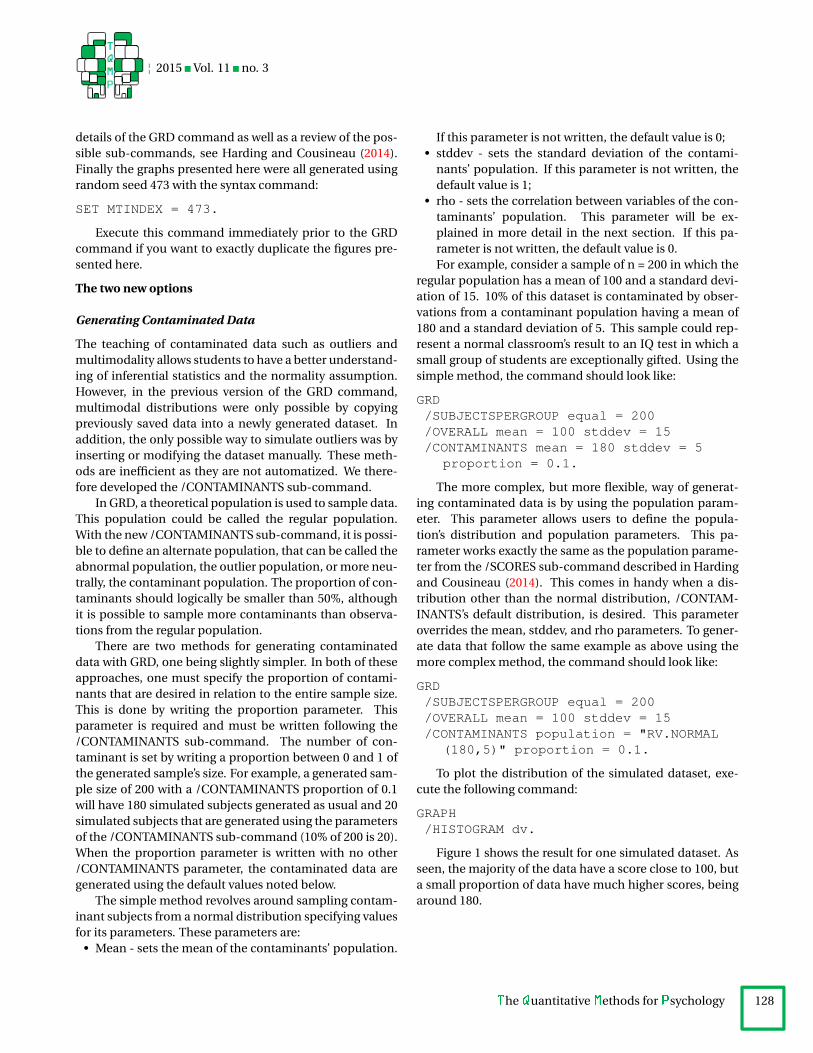
Figure 1 shows the result for one simulated dataset. Asseen, the majority of the data have a score close to 100, buta small proportion of data have much higher scores, beingaround 180.


¦ 2015 Vol. 11 no. 3

Figure 1 Histogram of a dataset with contaminated data as generated by the GRD command. The dataset was generatedwith a mean of 100, a standard deviation of 15, and a sample size of 200. The contaminated data is generated with a meanof 180, a standard deviation of 5 and represent a proportion of 10% of the full dataset (20 subjects generated with thecontaminants sub-command and 180 subjects generated as usual)

Generating Correlated Variables

Another aspect of GRD that was deemed missing is the abil-ity to simulate correlated variables. A correlation is definedas the proportion of data from one variable that follows thesame trend as another variable (Coladarci, Cobb, Minium,& Clarke, 2010) where the strength is interpreted by a num-ber between 1 and -1 with 0 being a null correlation. Tovisualize the strength of a correlation when there are twovariables, use a scatterplot in which the score of each vari-able is a coordinate on a grid. When all of the scores areplotted, the result is called a data cloud. This data cloud iswhat allows users to visualize correlation and estimate itsstrength and sign. Variables that are highly correlated havea data cloud that resembles a line. An upward-sloped linemeans that the variables are positively correlated and vice-versa. The data cloud of variables that are weakly corre-lated resembles a balloon with no clear trend. When thereare more than two variables, it is possible to generate scat-terplots for pairs of variables.

Correlated data can be sampled from multivariate dis-tributions in which the strength of the correlation is onepopulation parameter. Such multivariate distributions canbe symmetrical or not, have thick or thin surroundings(equivalent to a high or small kurtosis in a univariate dis-tribution), etc. However, as there is no multivariate distri-bution available in SPSS, we implemented one specificallyfor GRD. The parameters of this distribution are describedbelow.

There are two ways to implement correlated data inGRD. The simple way is to specify the rho parameter in the/OVERALL sub-command. This approach generates corre-lated data in a multivariate normal distribution where bothvariables have the same mean and standard deviation.

For example, consider the following syntax which gen-erates two variables with a mean of 100, a standard devi-ation of 15 that are correlated together with a rho of 0.9;note that the two correlated variables must be generated ina within-subject design:

GRD/SUBJECTSPERGROUP equal = 200/WSFACTORS Time (2)/OVERALL mean = 100 stddev = 15 rho =

0.9.

To plot the simulated dataset in a scatterplot, write thefollowing command:

GRAPH/SCATTERPLOT dv.1 with dv.2.

The scatterplot in Figure 2 shows a sample composedof two variables with an observed correlation of 0.907. Cor-relations can be measured with the CORRELATIONS com-mand, written as:

CORRELATIONS dv.1 dv.2.

The more complex way of simulating correlated dataallows for more control of the simulated dataset by using


¦ 2015 Vol. 11 no. 3

Figure 2 Scatterplot of correlated data with identical axes using the simple method of generating correlation, the rhoparameter. Both variables are generated with means of 100 and standard deviations of 15. The measured correlation iswritten in the top-left corner of the plot.

distinct means and distinct standard deviations for eachvariable. As was seen in the first version of the GRD com-mand (Harding & Cousineau, 2014), the population param-eter of the /SCORES sub-command allows users to sampledata from a specific population. In GRD 2.0, it is possi-ble to specify a multivariate normal distribution (this sub-command overrides the /OVERALL sub-command if it ispresent in the script) that will generate correlated variables.The multivariate normal distribution, noted RV.MVN, iswritten as

RV.MVN({means}, {covariance matrix})

in GRD syntax, where commas separate entries and semi-colons separate lines in the matrix.

To explain this distribution with more details, we con-centrate on the case with only two variables (a bivariatenormal distribution). This distribution is written as

RV.MVN({X,Y}, {s2X,covXY;covXY, s2

Y})

where we use X to denote the first variable and Y to denotethe second variable. This notation allows users to specifythe mean for each variable in the first set of brackets (notedas and for the means of X and Y respectively). The standarddeviations and correlation is found in the second set ofbrackets (a variance/covariance matrix). Although the vari-ance/covariance matrix allows for more complex datasetsthan simply writing rho, the notation is more complex aswell. The covariance matrix is equivalent to where is thevariance of X, is the variance of Y and is the covariance be-tween both variables. The correlation is found by dividing

the covariance by the product of both variables’ standarddeviation as shown in Equation 1:

rXY = covXY

sXsY(1)

where rX Y is the coefficient of correlation between bothvariables, is the covariance between X and Y and , are thestandard deviations of X and Y respectively. If we isolatethe covariance in (1) we get:

covXY = rXYsXsY (2)

Therefore, the variance/covariance matrix is equivalentto

{sX∗∗2,rXY

∗sX∗sY;rXY

∗sX∗sY, sY

∗∗2} (3)

The bivariate normal distribution then becomes:

RV.MVN({X,Y}, {sX∗∗2,rXY

∗sX∗sY;rXY

∗sX∗sY, sY

∗∗2}).

Negative correlations are generated by using a negativecovariance. In addition, in bivariate situations, it is imper-ative that the covariances in the matrix be equal to one an-other.

For example, to generate data where X has a mean of100, a standard deviation of 15, and Y has a mean of 200,a standard deviation of 20, with both variables correlatedwith r = 0.9, one would write 100, 200 for the means and asthe covariance matrix. The complete GRD script is thus:

GRD/SUBJECTSPERGROUP equal = 200/WSFACTORS Time (2)/SCORES population =


¦ 2015 Vol. 11 no. 3

"RV.MVN({100,200},{15**2,0.9*15*20;0.9*15*20,20**2})".

GRAPH/SCATTERPLOT dv.1 with dv.2.CORRELATIONS dv.1 dv.2.

Note that everything within quotes must appear on a singleline in the SPSS syntax editor.

One sample is shown in Figure 3. As seen, both vari-ables have different means as well as different standard de-viations. The measured correlation (r = 0.907) is shown inthe top-left corner of the plot.

Contaminants can also follow a multivariate normaldistribution. As aforementioned, /CONTAMINANTS hasthe rho parameter. When this parameter is present, thecorrelated contaminated data have the same proportion ofoutliers, the same mean, and the same standard deviationfor both variables. /CONTAMINANTS can also be sampledwith the population parameter. When the population pa-rameter is written, the notation is the same as that of the/SCORES population parameter written above. For exam-ple, if one were to contaminate 20% of the data presentedin Figure 3 with cases having a mean of 50 for X and 300 forY, a standard deviation of 10 and 5 for X and Y respectively,and a correlation of rho = 0.5 between both variables, onewould write the following:

GRD/SUBJECTSPERGROUP equal = 200/WSFACTORS Time (2)/SCORES population ="RV.MVN({100,200},{15**2,.9*15*20;.9*15*20,20**2})"

/CONTAMINANTS proportion = .2population ="RV.MVN({50,300},{10**2,.5*10*5;.5*10*5,5**2})".

GRAPH/SCATTERPLOT dv.1 with dv.2.


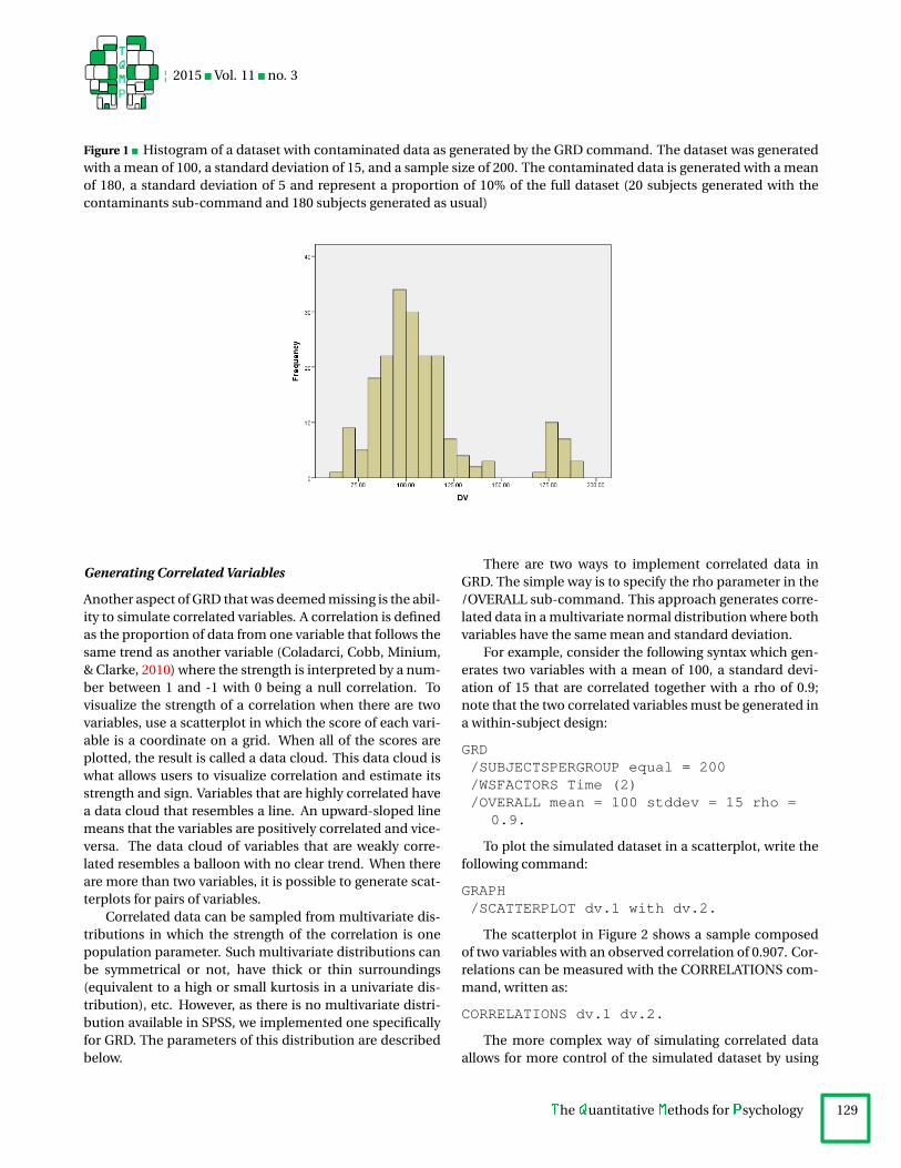
As seen in Figure 4, the majority of the data follows apositive correlation with a small set of data (the contami-nants) present in the top-left corner of the plot. Althoughthe data and contaminants have a strongly positive rela-tion on X and Y, the presence of the outliers makes for anoverall negative correlation (r = -0.516, noted in the top-right corner of the plot). This correlation is therefore un-interpretable as the whole dataset do not satisfy the nor-mality assumption.

Easier access to the GRD command

Syntax can be an overwhelming endeavor to learn for newstudents in statistics, especially when it is the student’s

first contact with SPSS. Therefore, we added a GUI to GRDto facilitate the use of random number generators in theclassroom. The new GUI for GRD is an intuitive alterna-tive to the written command that allows students to gen-erate a dataset by filling input fields rather than writingout a code. While we argue that syntax remains a toolworth learning for undergraduate students, occasional useof GRD might benefit from a more user-friendly interface (agraphical user interface, abbreviated GUI). All of the GRDsub-commands presented in this article as well as the onespresented in Harding and Cousineau (2014) are presentand accessible in this GUI.

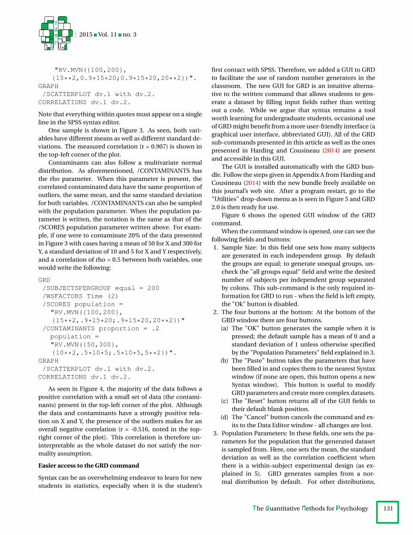
The GUI is installed automatically with the GRD bun-dle. Follow the steps given in Appendix A from Harding andCousineau (2014) with the new bundle freely available onthis journal’s web site. After a program restart, go to the"Utilities" drop-down menu as is seen in Figure 5 and GRD2.0 is then ready for use.

Figure 6 shows the opened GUI window of the GRDcommand.

When the command window is opened, one can see thefollowing fields and buttons:1. Sample Size: In this field one sets how many subjects

are generated in each independent group. By defaultthe groups are equal; to generate unequal groups, un-check the "all groups equal" field and write the desirednumber of subjects per independent group separatedby colons. This sub-command is the only required in-formation for GRD to run - when the field is left empty,the "Ok" button is disabled.

2. The four buttons at the bottom: At the bottom of theGRD window there are four buttons.(a) The "OK" button generates the sample when it is

pressed; the default sample has a mean of 0 and astandard deviation of 1 unless otherwise specifiedby the "Population Parameters" field explained in 3.

(b) The "Paste" button takes the parameters that havebeen filled in and copies them to the nearest Syntaxwindow (if none are open, this button opens a newSyntax window). This button is useful to modifyGRD parameters and create more complex datasets.

(c) The "Reset" button returns all of the GUI fields totheir default blank position.

(d) The "Cancel" button cancels the command and ex-its to the Data Editor window - all changes are lost.

3. Population Parameters: In these fields, one sets the pa-rameters for the population that the generated datasetis sampled from. Here, one sets the mean, the standarddeviation as well as the correlation coefficient whenthere is a within-subject experimental design (as ex-plained in 5). GRD generates samples from a nor-mal distribution by default. For other distributions,


¦ 2015 Vol. 11 no. 3

Figure 3 Scatterplot of correlated data with identical axes using the more complex method of generating correlation, thepopulation parameter. Variable 1 is generated with a mean of 100 and a standard deviation of 15 and variable 2 is gener-ated with a mean of 200 and a standard deviation of 20. The measured correlation is shown in the top-left corner of theplot.

press the "Optional" button explained in 6 or press the"Paste" button in the bottom of the window and adjustmanually in the syntax.

4. Between-Subject Factors: This field allows users to gen-erate a between-subject experimental design. Userscan specify a name as well as how many groups eachfactor has. In the GUI, users can create up to two differ-ent between-subject factors. If more factors are needed,press the "Paste" button and add more manually in thesyntax. However, GRD can only generate a maximum of4 different factors (regardless of if they are between- orwithin-subject factors)

5. Within-Subject Factors: This field allows users to gen-erate a within-subject experimental design. Users canspecify a name as well as how many repeated measureseach factor has. In the GUI, users can create up totwo different within-subject factors. If more factors areneeded, likewise use the "Paste" button. Again, GRDcan only generate a maximum of 4 different factors (re-gardless of if they are between- or within-subject fac-tors)

6. Optional Buttons on the right: In this dialog window,users have access to:(a) The "Random Seed" field where one can choose a

specific seed to be generated.(b) The "Population Function" field allows users to

manually change the population’s shape. When thisfield is filled, it overrides the "Population Parame-ters" fields from 3.

(c) The "Print Information" checkboxes allow users to

get information on the "Debug information", the"GRD version", and the "Full Instruction Gener-ated". These technical commands are new in GRD2.0 and are explained further in Appendix A. There isalso the option to print the "Effect Size Table" whichallows users to print the population effect size wheneffects are defined (see 8).

7. Contaminants Button: This button on the main win-dow brings users to a dialog window where one can addcontaminants do the data. Here one sets the proportionof contaminants, the mean, the standard deviation, andthe correlation coefficient for the contaminant popula-tion. Again, when the rho field is filled out, there needsto be a within-subject experimental design. There isalso the option to set the contaminants’ population’sdistribution. When this parameter is filled out, it over-rides the other three contaminants’ population shapeparameters.

8. Define Effects: This button on the main window bringsusers to a dialog window where it is possible to addan effect to a factor. In the "Factor Name" field, onewrites the name of the between- or within-subject fac-tor where an effect is desired. The factor’s name mustbe written exactly the same as it is in GRD’s main win-dow. In the "Effect-Type" drop down menu one setswhat type of effect is desired. In the "Value" entry field,one sets the value of the factor’s effect. It is possibleto add a total of two effects on the four possible gener-ated factors. To add more than two effects, modify theGRD syntax manually. For more information on the ef-


¦ 2015 Vol. 11 no. 3

Figure 4 Scatterplot of a dataset generated with contaminated data. In the top-left of the data cloud, there is contami-nated data that was generated using the population parameter. As is seen, the presence of the contaminated data heavilyskews the correlation (in the top-left corner of the plot) of an otherwise well-correlated dataset.

Figure 5 Where GRD is nested in the drop-down menu.


¦ 2015 Vol. 11 no. 3

Figure 6 GRD GUI window as well as the dialog windows associated with each button.

fect types and their characteristics, consult Harding andCousineau (2014).

Exercises

In this section we present a series of exercises for GRD thatcan be implemented in a classroom setting. We first pro-vide context to why the exercise is important followed bythe Syntax and GUI inputs for each (both options can besimply copied and pasted into their respective SPSS win-dow). In these exercises, the parameters we propose areguidelines and there exist a variety of strategies to imple-ment each. In addition, we encourage teachers to createtheir own exercises and encourage an active learning class-room, as is recommended by the GAISE College Report(American Statistical Association et al., 2005, recommen-dation 4).

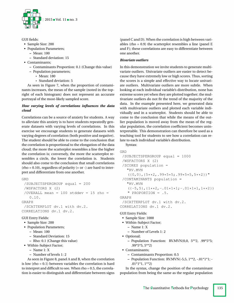
How contaminated data affect descriptive statistics

An exercise to show how contaminants affect the descrip-tive statistics of a dataset is to have students generatedatasets with varying levels of imperfection; encouragingstudents to see that every decision made on a sample mustbe made with a critical eye. For example, samples thatdo not respect the normality assumption cannot be stud-ied with standard descriptive statistics. In this exercise,we encourage students to generate datasets with varying

proportions of contaminants (10%, 25%, and 50%) andnote the mean of the sample. The mean is supposed toshow the representative score of a dataset, the score that ismost likely to be sampled (Watier, Lamontagne, & Chartier,2011). When outliers are present, the measured mean doesnot reflect the score that is most likely to be sampled asthe mean is not a robust statistic (Harding, Tremblay, &Cousineau, 2014); especially when the outliers are far awayfrom the central peak of the distribution. Students shouldbe able to see the change in the mean as the proportion ofcontaminants increases and come to the conclusion thatthe mean is not accurately portraying the central tendency.Students should also be able to come to the conclusion thatthe normality assumption is essential for the interpretationof descriptive statistics.

GRD/SUBJECTSPERGROUP equal = 200/OVERALL mean = 100 stddev = 15/CONTAMINANTS mean = 180 stddev = 5

proportion = 0.1.GRAPH/HISTOGRAM dv.

where the mean is measured with:

MEANS dv.


¦ 2015 Vol. 11 no. 3

GUI fields:• Sample Size: 200• Population Parameters;

– Mean: 100– Standard deviation: 15

• Contaminants;– Contaminants Proportion: 0.1 (Change this value)– Population parameters;

* Mean: 180

* Standard deviation: 5As seen in Figure 7, when the proportion of contami-

nants increases, the mean of the sample (noted in the top-right of each histogram) does not represent an accurateportrayal of the most-likely sampled score.

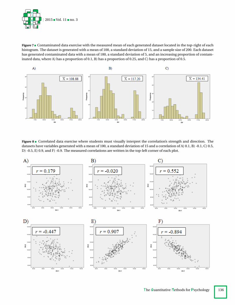
How varying levels of correlations influences the datacloud

Correlations can be a source of anxiety for students. A wayto alleviate this anxiety is to have students repeatedly gen-erate datasets with varying levels of correlations. In thisexercise we encourage students to generate datasets withvarying degrees of correlation (both positive and negative).The student should be able to come to the conclusion thatthe correlation is proportional to the elongation of the datacloud; the more the scatterplot resembles a line the higherthe correlation is; conversely, the more the scatterplot re-sembles a circle, the lower the correlation is. Studentsshould also come to the conclusion that small correlations(rho = 0.10), regardless of polarity (+ or -) are hard to inter-pret and differentiate from one another.

GRD/SUBJECTSPERGROUP equal = 200/WSFACTORS X (2)/OVERALL mean = 100 stddev = 15 rho =

0.10.GRAPH/SCATTERPLOT dv.1 with dv.2.


GUI Entry Fields:• Sample Size: 200• Population Parameters;

– Mean: 100– Standard Deviation: 15– Rho: 0.1 (Change this value)

• Within-Subject Factor;– Name 1: X– Number of levels 1: 2

As seen in Figure 8, panel A and B, when the correlationis low (rho = 0.1) between variables the correlation is hardto interpret and difficult to see. When rho = 0.5, the correla-tion is easier to distinguish and differentiate between signs

(panel C and D). When the correlation is high between vari-ables (rho = 0.9) the scatterplot resembles a line (panel Eand F); these correlations are easy to differentiate betweenone another.

Bivariate outliers

In this demonstration we invite students to generate multi-variate outliers. Univariate outliers are easier to detect be-cause they have extremely low or high scores. Thus, sortingthe scores is a simple and effective way to locate univari-ate outliers. Multivariate outliers are more subtle. Whenlooking at each individual variable’s distribution, none hasextreme scores yet when they are plotted together; the mul-tivariate outliers do not fit the trend of the majority of thedata. In the example presented here, we generated datawith multivariate outliers and plotted each variable indi-vidually and in a scatterplot. Students should be able tocome to the conclusion that while the means of the out-lier population is moved away from the mean of the reg-ular population, the correlation coefficient becomes unin-terpretable. This demonstration can therefore be used as ateaching tool for students to see how a correlation can re-late to each individual variable’s distribution.

Syntax:

GRD/SUBJECTSPERGROUP equal = 1000/WSFACTORS X (2)/SCORES population =

"RV.MVN({0,0},{5**2,.99*5*5;.99*5*5,5**2})"

/CONTAMINANTS population ="RV.MVN({-5,5},{1**2,-.01*1*1;-.01*1*1,1**2})" PROPORTION = .5.

GRAPH/SCATTERPLOT dv.1 with dv.2.CORRELATIONS dv.1 dv.2.

GUI Entry Fields:• Sample Size: 1000• Within-Subject Factor;

– Name 1: X– Number of Levels 1: 2

• Optional;– Population Function: RV.MVN(0,0, 5**2, .99*5*5;

.99*5*5, 5**2)• Contaminants;

– Contaminants Proportion: 0.5– Population Function: RV.MVN(-5,5, 1**2, -.01*1*1; -

.01*1*1, 1**2)In the syntax, change the position of the contaminant

population from being the same as the regular population


¦ 2015 Vol. 11 no. 3

Figure 7 Contaminated data exercise with the measured mean of each generated dataset located in the top-right of eachhistogram. The dataset is generated with a mean of 100, a standard deviation of 15, and a sample size of 200. Each datasethas generated contaminated data with a mean of 180, a standard deviation of 5, and an increasing proportion of contam-inated data, where A) has a proportion of 0.1, B) has a proportion of 0.25, and C) has a proportion of 0.5.

Figure 8 Correlated data exercise where students must visually interpret the correlation’s strength and direction. Thedatasets have variables generated with a mean of 100, a standard deviation of 15 and a correlation of A) 0.1, B) -0.1, C) 0.5,D) -0.5, E) 0.9, and F) -0.9. The measured correlations are written in the top-left corner of each plot.


¦ 2015 Vol. 11 no. 3

Figure 9 Figure 9. Example of multivariate outliers where each individual variable respects the normality assumption yetgo against the homogeneity of variance assumption when paired. Panel A shows the histogram for the first variable, B) thehistogram for the second variable, and C) the scatterplot for both.

0,0 to much different -5,5 by increment of 1 (i.e., 0,0, -1,1,-2,2, etc.). At what point do the multivariate outliers influ-ence markedly the correlation? Are they easily detected ona scatter plot?

Conclusion

Here we presented two new options to GRD as well as anoverview of a GUI. This update to the GRD command ad-dresses comments made by users of the first version of GRD(Harding & Cousineau, 2014). We also provided a series ofexercises that aim to inspire teachers and students alike tothink of statistics as a series of constructs rather than sim-ply as equations written on a page.

References

American Statistical Association, Aliaga, M., Cobb, G., Cuff,C., Garfield, J., Gould, R., . . . Witmer, J. (2005). Guide-

lines for assessment and instruction in statistics edu-cation [gaise] college report. Alexandria, VA.: Ameri-can Statistical Association.

Coladarci, T., Cobb, C. D., Minium, E. W., & Clarke, R. C.(2010). Fundamentals of statistical reasoning in edu-cation (3rd ed.). Hoboken, NJ: John Wiley & Sons.

Harding, B. & Cousineau, D. (2014). GRD: an SPSS ex-tension command for generating random data. TheQuantitative Methods for Psychology, 10(2), 80–94.

Harding, B., Tremblay, C., & Cousineau, D. (2014). Standarderrors: a review and evaluation of standard error es-timators using monte carlo simulations. The Quanti-tative Methods for Psychology, 10(2), 107–123.

Watier, N., Lamontagne, C., & Chartier, S. (2011). Whatdoes the mean mean? Journal of Statistics Education,19(2), 1–20.

Appendix A: Technical sub-command for GRD

Here we show how to use technical sub-commands for GRD that allow users to delve deeper in the command’s innerworkings. In this section we give a short description of these sub-commands as well as their Syntax - they are all nestedunder the /PRINT sub-command. These commands are also available in the "Optional Sub-commands" side window ofthe GUI as checkboxes as explained in the second section of this tutorial.

PRINT version

Here one can check which version of GRD is installed. This command comes in handy when one wants to verify thatthe command is installed properly. For users of the first version of GRD, this command is useful to make sure that thenew version of GRD is installed. It also displays copyright information and how to cite the command if necessary. Thesub-command should be added in SPSS Syntax like this:

.../PRINT version...


¦ 2015 Vol. 11 no. 3

PRINT debug

Here one can check if the sub-commands are running properly. When this command is present, the Output window forSPSS shows each of the individual sub-commands and if they have successfully parsed. This command could be useful ifone has made a mistake in generation of a complex dataset and cannot find where the error has occurred.

.../PRINT debug...

PRINT fullinstructions

Here one can see the steps that GRD goes through to generate a dataset. When this command is written, the SPSS Outputfile shows a series of code that is the backbone of GRD. This sub-command is useful for users who wish to see the innerworkings of the command and be inspired to create extension commands of their own.

.../PRINT fullinstructions...

PRINT es

Here one can see the effect size table of a dataset generated by GRD. For this sub-command to run, it is imperative that aneffect has been requested on at least one of the experimental design’s factors; if no effects are requested, this commanddoes not return any results. When an effect is specified, the generated table shows the synopsis of each group’s change inmean in relation the population parameters set in the command. For example, a factor generated with a mean of 100 andan effect size of 10 signifies that that factor’s group has a generated mean of 110 (100+10). All factors are noted in the tablealong with each factor’s group’s effect size is separated by a comma.

.../PRINT es...

Citation

Harding, B., & Cousineau, D. (2015) GRD 2.0: An extended SPSS extension command for generating random data. TheQuantitative Methods for Psychology, 11(3), 127-138.

Copyright © 2015 Harding & Cousineau. This is an open-access article distributed under the terms of the Creative Commons Attribution License (CC

BY). The use, distribution or reproduction in other forums is permitted, provided the original author(s) or licensor are credited and that the original

publication in this journal is cited, in accordance with accepted academic practice. No use, distribution or reproduction is permitted which does not

comply with these terms.

Received: 20/07/2015


GRD 2.0: An extended SPSS extension command for generating ... · ¦2015 Vol. 11 no. 3 GRD 2.0: An...

Documents

Transcript of GRD 2.0: An extended SPSS extension command for generating ... · ¦2015 Vol. 11 no. 3 GRD 2.0: An...