gravity method

Tom Wilson, Department of Geology and Geography

Environmental and Exploration Geophysics II

tom.h. wilson

[email protected]

Department of Geology and Geography

West Virginia University

Morgantown, WV

Gravity Methods (II)

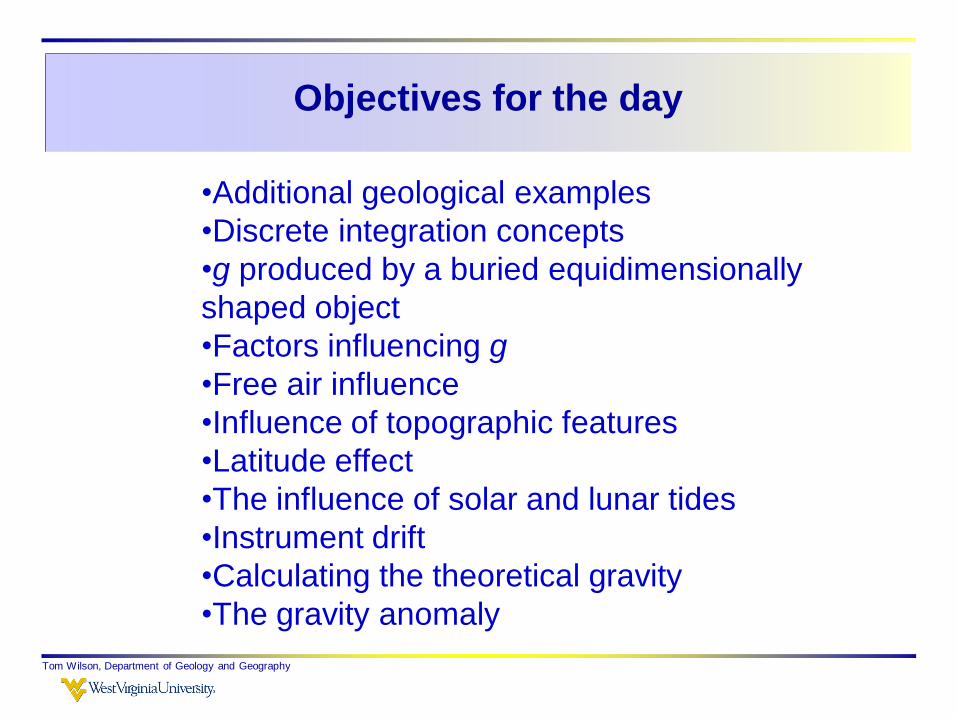
Objectives for the day


•Additional geological examples

•Discrete integration concepts

•g produced by a buried equidimensionally

shaped object

•Factors influencing g

•Free air influence

•Influence of topographic features

•Latitude effect

•The influence of solar and lunar tides

•Instrument drift

•Calculating the theoretical gravity

•The gravity anomaly


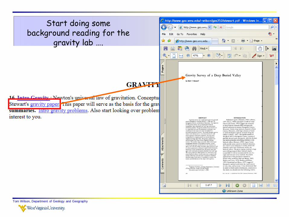
Start doing some background reading for the

gravity lab ….


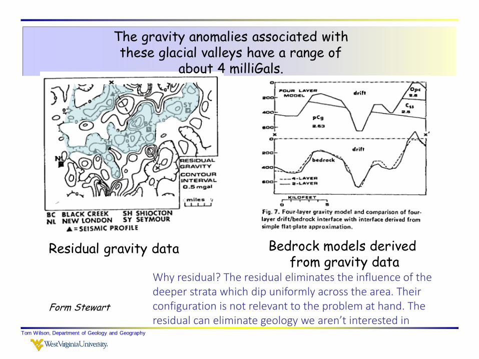
Form Stewart

Bedrock models derived from gravity data

Residual gravity data

The gravity anomalies associated with these glacial valleys have a range of

about 4 milliGals.

Why residual? The residual eliminates the influence of the deeper strata which dip uniformly across the area. Their configuration is not relevant to the problem at hand. The residual can eliminate geology we aren’t interested in

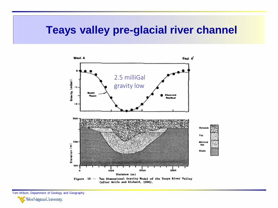
Teays valley pre-glacial river channel


2.5 milliGal gravity low


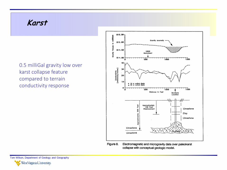
Karst

0.5 milliGal gravity low over karst collapse feature compared to terrain conductivity response


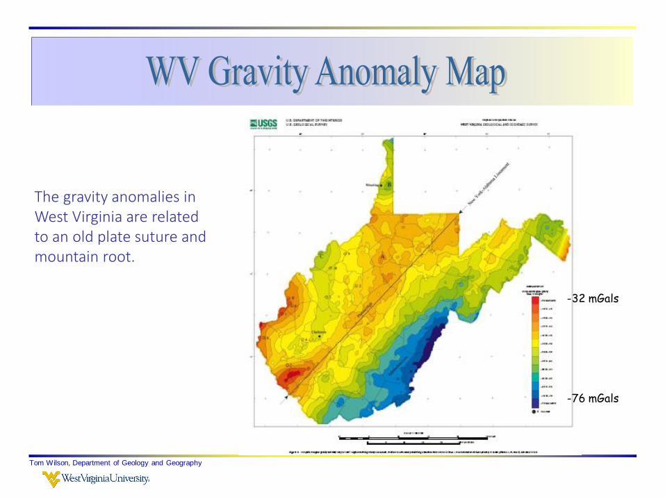
-76 mGals

-32 mGals

The gravity anomalies in West Virginia are related to an old plate suture and mountain root.

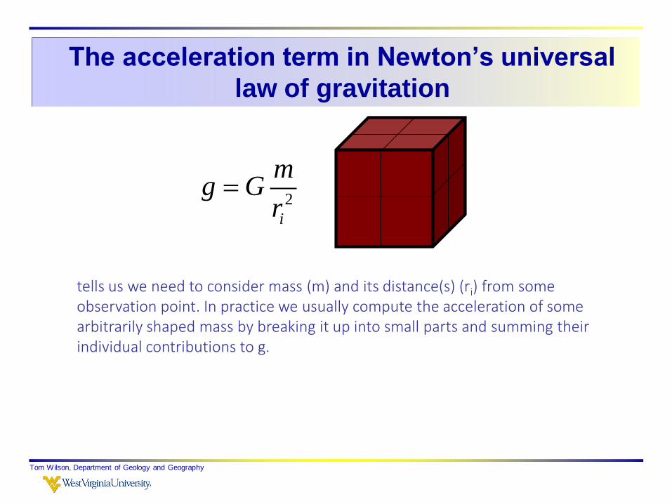
The acceleration term in Newton’s universal

law of gravitation


2

i

mg G

r

tells us we need to consider mass (m) and its distance(s) (ri) from some observation point. In practice we usually compute the acceleration of some arbitrarily shaped mass by breaking it up into small parts and summing their individual contributions to g.


2, , or L S V

Gdmg

r

Integral form of Newton’s law of gravitation

Line, surface or volume

Depending on symmetry

2

G dVg

r

2

G dxdydzg

r

dz

dy

dx

dV


Just as a footnote, Newton had to develop the mathematical methods of calculus to show that spherically symmetrical objects gravitate as though all their mass is concentrated at their center.


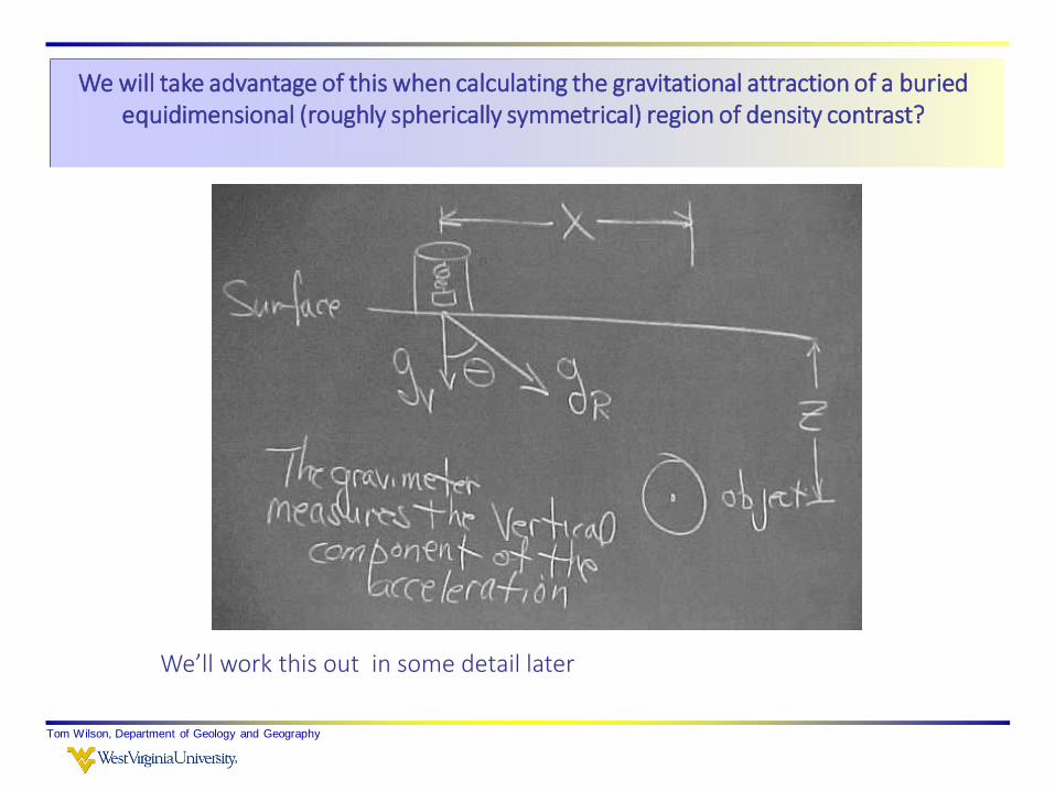
We will take advantage of this when calculating the gravitational attraction of a buried equidimensional (roughly spherically symmetrical) region of density contrast?

We’ll work this out in some detail later

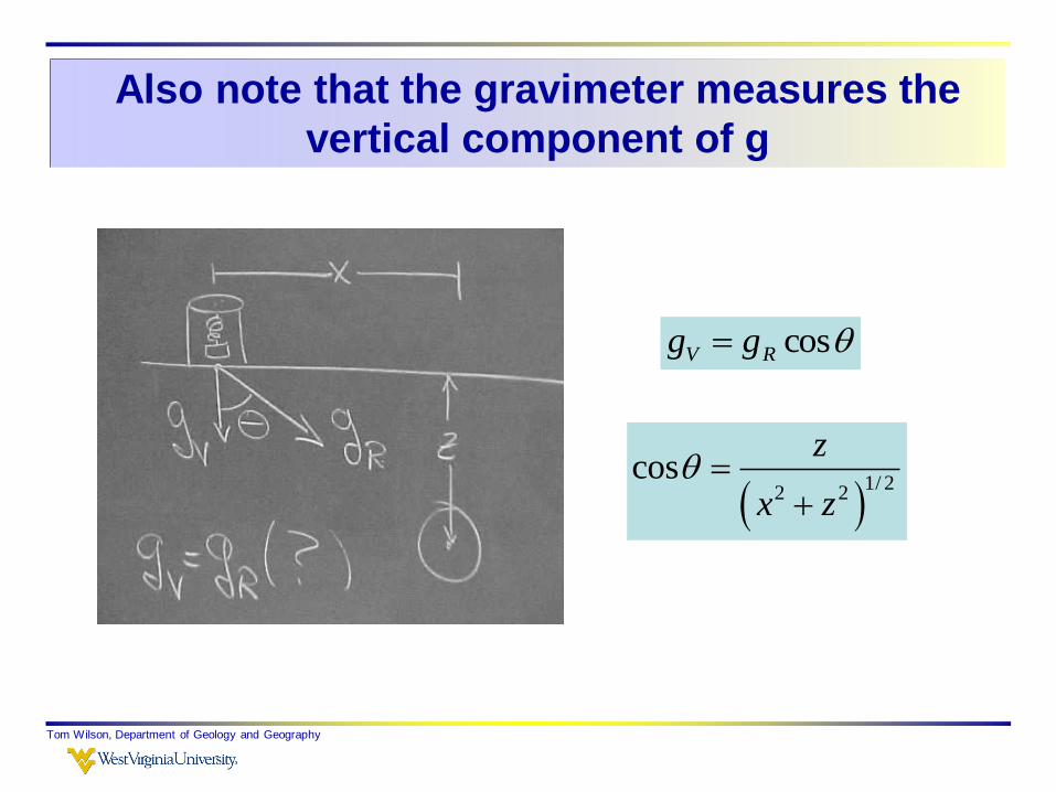
Also note that the gravimeter measures the

vertical component of g


cosRV gg

1/ 2

2 2cos

z

x z

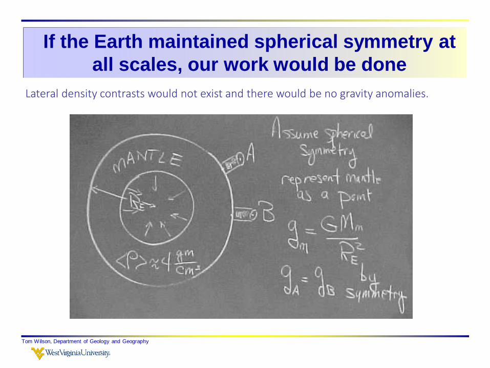
If the Earth maintained spherical symmetry at

all scales, our work would be done


Lateral density contrasts would not exist and there would be no gravity anomalies.


How thick is the landfill?

Gravity methods thrive on heterogeneity. In general the objects we are interested in are not so symmetrical and provide us with considerable lateral density contrast and thus gravity anomalies.

How does g vary from point A to E across the

landfill?


We might expect that the average density of materials in the landfill would be less than that of the surrounding bedrock and thus be an area of lower g, where g

would vary in proportion to


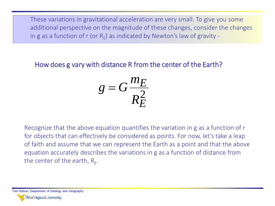
These variations in gravitational acceleration are very small. To give you some additional perspective on the magnitude of these changes, consider the changes in g as a function of r (or RE) as indicated by Newton’s law of gravity -

2E

E

R

mGg

Recognize that the above equation quantifies the variation in g as a function of r for objects that can effectively be considered as points. For now, let’s take a leap of faith and assume that we can represent the Earth as a point and that the above equation accurately describes the variations in g as a function of distance from the center of the earth, RE.

How does g vary with distance R from the center of the Earth?


2E

Esl

R

mGg Given this relationship -

RE

hWhat is g at a distance RE+h from the center of the earth?

sl=sea level

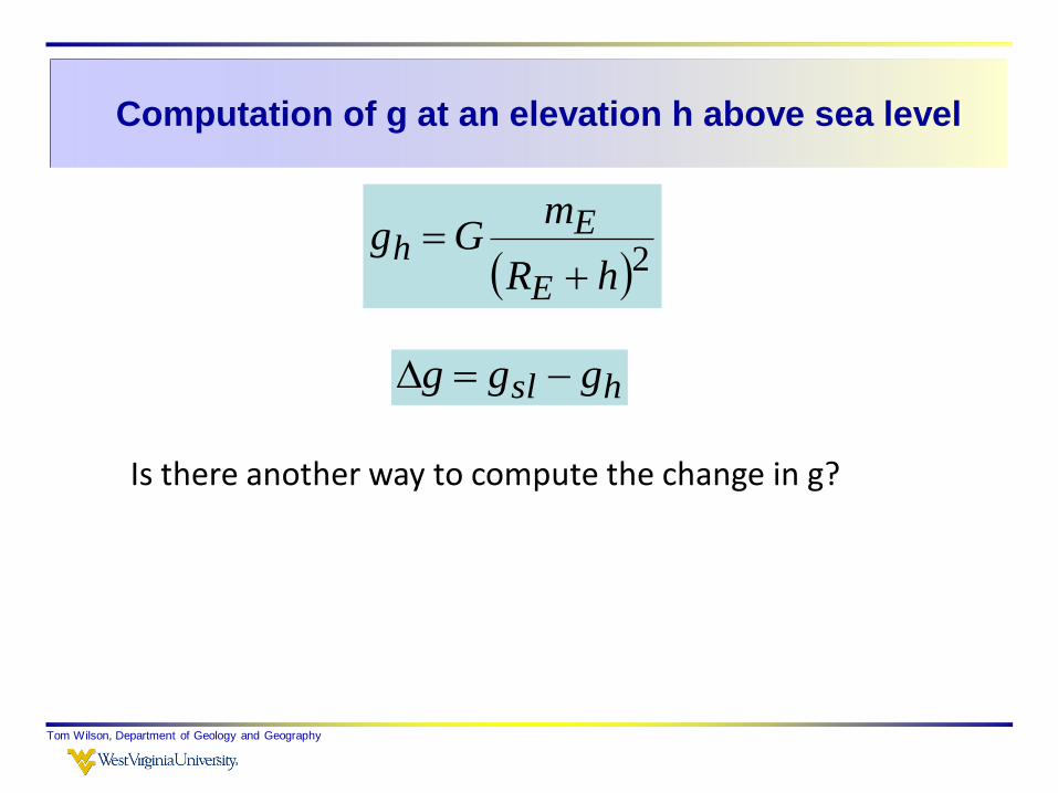
Computation of g at an elevation h above sea level


2hR

mGg

E

Eh

hsl ggg

Is there another way to compute the change in g?


2E

E

R

mGg What does the derivative of

g with respect to R provide?

2E

E

R

mG

dR

d

dR

dg

2 EE RdR

dGm

dR

dg

g/h - in Morgantown


At Morgantown latitudes, the variation of g with elevation is approximately 0.3086 milligals/m or approximately 0.09406 milligals/foot.

As you might expect, knowing and correcting for elevation differences between gravity observation points is critical to the interpretation and modeling of gravity data.

The anomalies associated with the karst collapse feature were of the order of 1/2 milligal so an error in elevation of 2 meters would yield a difference in g greater than that associated with the density contrasts around the collapsed area.


•How do we compensate for the influence of matter between the observation point (A) and sea level?

•How do we compensate for the irregularities in the earth’s surface - its topography?

A hill will take us down the gravity ladder, but as we walk uphill, the mass beneath our feet adds to g.


What other effects do we need to consider?

Latitude effect

463 meters/sec

~1000 mph

Centrifugal acceleration carries you around the Earth with velocity

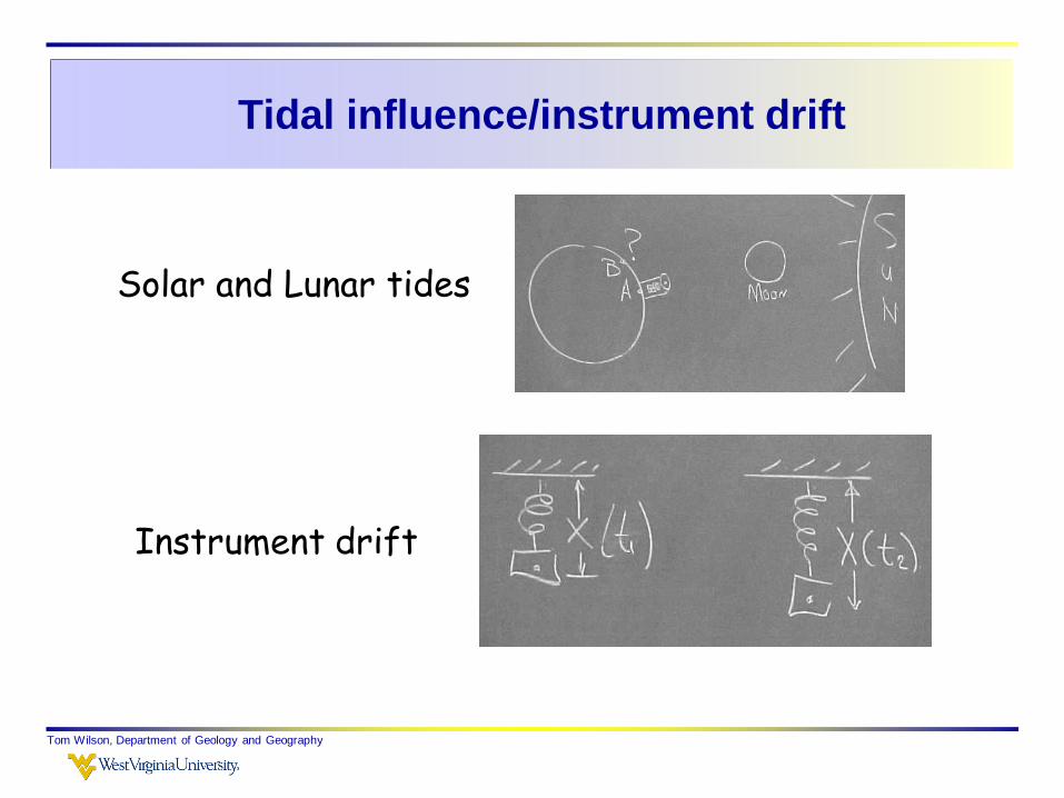
Tidal influence/instrument drift


Solar and Lunar tides

Instrument drift

Making a prediction of g at any location on Earth


To conceptualize the dependence of gravitational acceleration on various factors, we usually write g as a sum of different influences or contributions.

These are -

Terms in the predicted or theoretical g at a

given location.


Terms include:

gn the normal gravity of the gravitational acceleration on the reference

ellipsoid

gFA the elevation or free air effect

gB the Bouguer plate effect or the contribution to measured or observed g

of the material between sea-level and the elevation of the observation

point

gT the effect of terrain on the observed g

gTide and Drift the effects of tide and drift (often combined)

These different terms can be combined into an expression which is

equivalent to the prediction of what the acceleration should be at any

particular observation point on the surface of a homogeneous earth.

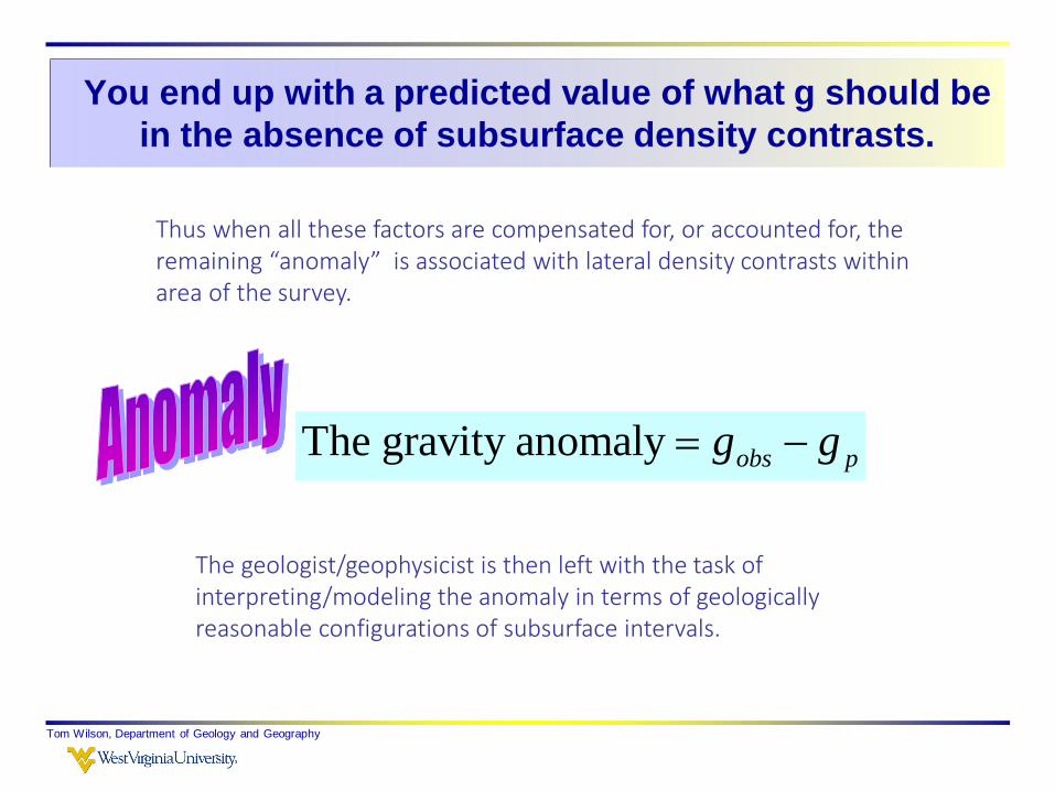
You end up with a predicted value of what g should be

in the absence of subsurface density contrasts.


Thus when all these factors are compensated for, or accounted for, the remaining “anomaly” is associated with lateral density contrasts within area of the survey.

The geologist/geophysicist is then left with the task of interpreting/modeling the anomaly in terms of geologically reasonable configurations of subsurface intervals.

The gravity anomaly obs pg g

The theoretical or predicted

acceleration as a formula


That predicted, estimated or theoretical value of g, gt, (or predicted value, gp, they are the same) is expressed as follows:

If the observed values of g behave according to this ideal model (i.e. if go=gp) then there is no complexity in the geology! - i.e. no lateral density contrasts. The geology would be fairly uninteresting - a layer cake ...

Let’s look at the individual terms in this expression.

( )p n FA B t Tide Driftg g g g g g


What is the centrifugal acceleration at the equator?

460sec

eq

mv

2

20.033

sec

v ma

R

3300 milligals

21distance = 2

at

Although that acceleration is small, if you were subjected only to that acceleration, you would fall 0.4 meters in 5 seconds

1.65 meters in 10 seconds

The centrifugal acceleration alone is about 6 times the acceleration of gravity on Phobos.

with


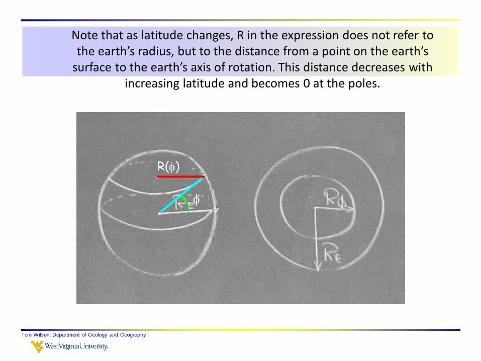
Note that as latitude changes, R in the expression does not refer to the earth’s radius, but to the distance from a point on the earth’s

surface to the earth’s axis of rotation. This distance decreases with increasing latitude and becomes 0 at the poles.

R()


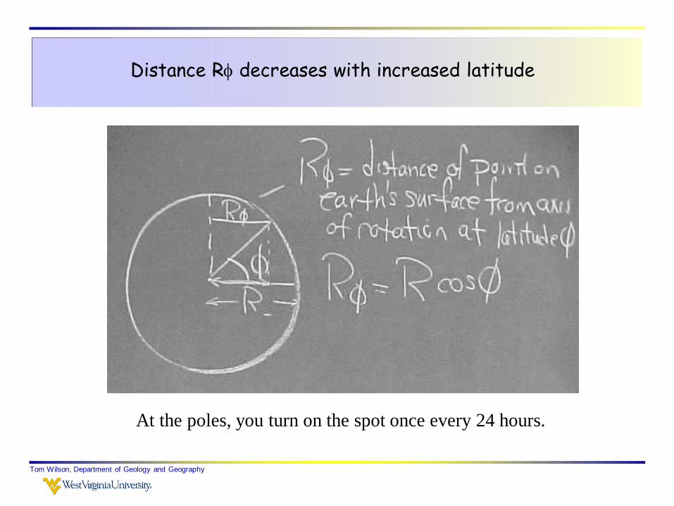
Distance R decreases with increased latitude

At the poles, you turn on the spot once every 24 hours.


The combined effects of the earth’s shape and centrifugal acceleration are represented as a function of latitude (). The formula below was adopted as a standard by the International Association of Geodesy in 1967. The formula is referred to as the Geodetic Reference System formula of 1967 or GRS67

2 421 sin sinn e

cmg g A Bs

2 42978.03185 1 0.005278895sin 0.000023462sinn

cmg gs

gn() incorporates latitude effects

See page 357, eqn. 6.12 -Burger et al. 2006

2 421 sin sino

cmg gs

Familiarize yourself with the units discussed

earlier


Remember the gravity unit (otherwise known as gu)?

Recall that the milliGals represent 10-5 m/sec2

The milliGal is referenced to the Gal. In

recent years, the gravity unit (gu) has

become popular, largely because

instruments have become more sensitive and

it’s reference is to meters/sec2 i.e. 10-6

m/sec2 or 1 micrometer/sec2.


mile

milligalgn

2sin307.1

The gradient of this effect is

This is a useful expression, since you need only go through the calculation of GRS67 once in a particular survey area. All other estimates of gn can be made by adjusting the value according to the above formula.

The accuracy of your survey can be affected by an imprecise knowledge of one’s actual latitude. The above formula reveals that an error of 1 mile in latitude translates into an error of 1.31 milliGals (13.1 gu) at a latitude of 45o (in Morgantown (about 40oN, this gradient is 12.84 gu/mile).

The accuracy you need in your position latitude depends in a practical sense on the change in acceleration you are trying to detect.

2 42978.03185 1 0.005278895sin 0.000023462sinn

cmg gs


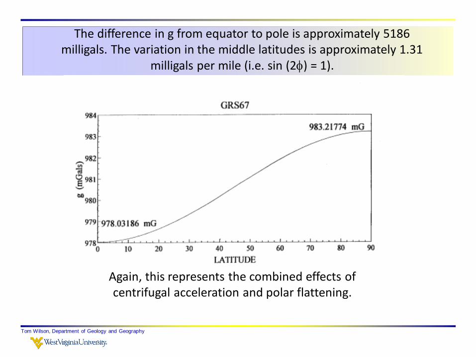
The difference in g from equator to pole is approximately 5186 milligals. The variation in the middle latitudes is approximately 1.31

milligals per mile (i.e. sin (2) = 1).

Again, this represents the combined effects of centrifugal acceleration and polar flattening.


The next term in our expression of the theoretical gravity is gFA - the free air term.

In our earlier discussion we showed that dg/dR could be approximated as -2g/R.

Using an average radius for the earth this turned out to be about 0.3081 milligals/m (about 3 gu).

( )t n B t Tide DFA riftg g g gg g

gFA - Free air term

Ignore the last two terms and multiply both

sides by R (or h) to get g


zR

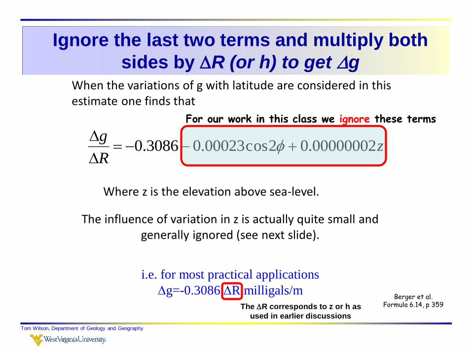
g00000002.02cos00023.03086.0

When the variations of g with latitude are considered in this estimate one finds that

Where z is the elevation above sea-level.

The influence of variation in z is actually quite small and generally ignored (see next slide).

i.e. for most practical applications

g=-0.3086 R milligals/mBerger et al.

Formula 6.14, p 359

For our work in this class we ignore these terms

The R corresponds to z or h as

used in earlier discussions


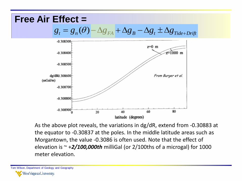
As the above plot reveals, the variations in dg/dR, extend from -0.30883 at the equator to -0.30837 at the poles. In the middle latitude areas such as Morgantown, the value -0.3086 is often used. Note that the effect of elevation is ~ +2/100,000th milliGal (or 2/100ths of a microgal) for 1000 meter elevation.

Free Air Effect =

From Burger et al.

( )t n FA B t Tide Driftg g g g g g


The variation of dg/dR with elevation - as you can see in the above graph - is quite small.

From Burger et al.

0.3086 where z = Rg z

So, again, for our work in class, we will ignore the second and third terms and calculate the change in acceleration with change in elevation as

Compensating for matter between your

observation point and sea level


This is a two-step process that involves treating the influence of materials beneath the surface as resulting from a featureless flat blanket of material having a thickness equal to the elevation above sea level, with the influence of topographic features introduced in a second step.

Two corrections are required: the plate correction and the topographic correction.


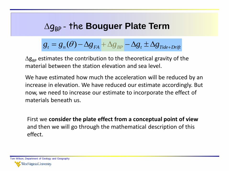
gBP estimates the contribution to the theoretical gravity of the material between the station elevation and sea level.

We have estimated how much the acceleration will be reduced by an increase in elevation. We have reduced our estimate accordingly. But now, we need to increase our estimate to incorporate the effect of materials beneath us.

First we consider the plate effect from a conceptual point of viewand then we will go through the mathematical description of this effect.

( )t n FA BP t Tide Driftg g g g g g

gBP – the Bouguer Plate Term

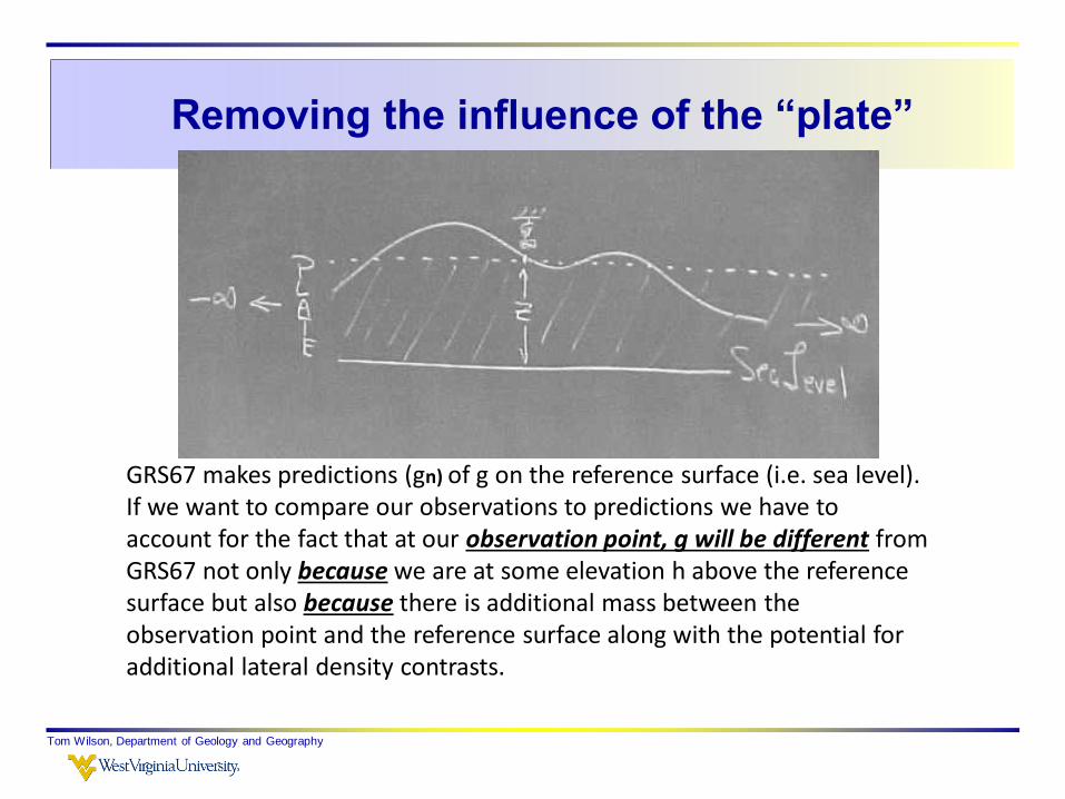
Removing the influence of the “plate”


GRS67 makes predictions (gn) of g on the reference surface (i.e. sea level). If we want to compare our observations to predictions we have to account for the fact that at our observation point, g will be different from GRS67 not only because we are at some elevation h above the reference surface but also because there is additional mass between the observation point and the reference surface along with the potential for additional lateral density contrasts.

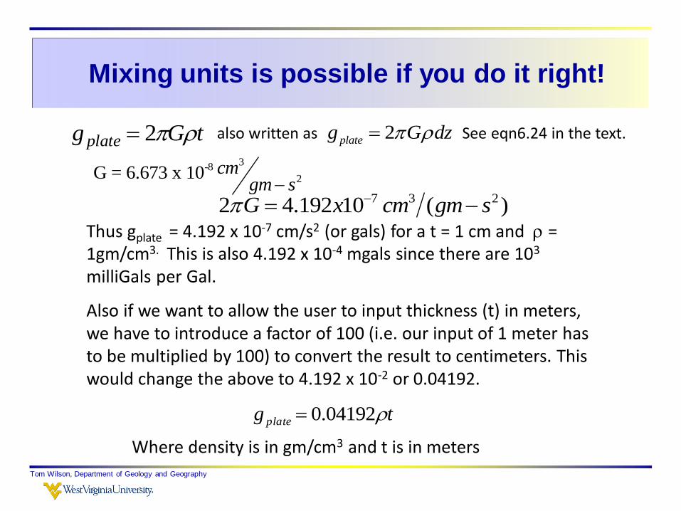
Mixing units is possible if you do it right!


2plateg G dz

3-8

2G = 6.673 x 10 cmgm s

7 3 22 4.192 10 ( )G x cm gm s Thus gplate = 4.192 x 10-7 cm/s2 (or gals) for a t = 1 cm and = 1gm/cm3. This is also 4.192 x 10-4 mgals since there are 103

milliGals per Gal.

Also if we want to allow the user to input thickness (t) in meters, we have to introduce a factor of 100 (i.e. our input of 1 meter has to be multiplied by 100) to convert the result to centimeters. This would change the above to 4.192 x 10-2 or 0.04192.

tg plate 04192.0

Where density is in gm/cm3 and t is in meters

tGg plate 2 also written as See eqn6.24 in the text.


gB may seem like a pretty unrealistic approximation of the topographic

surface. It is! You had to scrape off all mountain tops above the observation

elevation and fill in all the valleys when you made the plate correction.

( )t n FA B t Tide Driftg g g g g g

Topographic effects

See figure 6.3


So - now we have to carve out those valleys and put the hills back.

We compute their influence on gt ….

to compensate for the effect of topography on the plate.

Valleys and Hills

What is the effect of a topographic feature

such as a hill or valley


In either case, the influence is to decrease the local

acceleration due to gravity

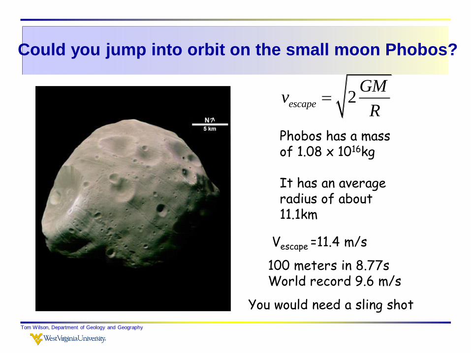
Could you jump into orbit on the small moon Phobos?


2escape

GMv

R

Phobos has a mass of 1.08 x 1016kg

It has an average radius of about 11.1km

Vescape =11.4 m/s

100 meters in 8.77sWorld record 9.6 m/s

You would need a sling shot


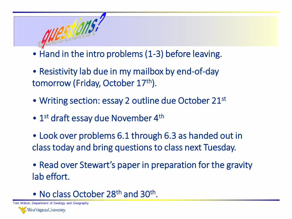
• Hand in the intro problems (1-3) before leaving.

• Resistivity lab due in my mailbox by end-of-day tomorrow (Friday, October 17th).

• Writing section: essay 2 outline due October 21st

• 1st draft essay due November 4th

• Look over problems 6.1 through 6.3 as handed out in class today and bring questions to class next Tuesday.

• Read over Stewart’s paper in preparation for the gravity lab effort.

• No class October 28th and 30th.

gravity method

Documents

Transcript of gravity method