sid.inpe.br/mtc-m19/2012/04.17.15.03-MAN

GRAVITATIONAL WAVE ANTENNA MARIO

SCHENBERG: MANUAL OF THE DATA ACQUISITION

SYSTEM

Carlos Filipe da Silva Costa

Cesar Strauss

Cesar Augusto Costa

Technical manual: instructions of

use and installation of the data ac-

quisition system.

URL of the original document:

<http://urlib.net/8JMKD3MGP7W/3BNEMBL>

INPE

Sao Jose dos Campos

2012

PUBLISHED BY:

Instituto Nacional de Pesquisas Espaciais - INPE

Gabinete do Diretor (GB)

Servico de Informacao e Documentacao (SID)

Caixa Postal 515 - CEP 12.245-970

Sao Jose dos Campos - SP - Brasil

Tel.:(012) 3208-6923/6921

Fax: (012) 3208-6919

E-mail: pubtc@sid.inpe.br

BOARD OF PUBLISHING AND PRESERVATION OF INPE INTEL-

LECTUAL PRODUCTION (RE/DIR-204):

Chairperson:

Marciana Leite Ribeiro - Servico de Informacao e Documentacao (SID)

Members:

Dr. Antonio Fernando Bertachini de Almeida Prado - Coordenacao Engenharia e

Tecnologia Espacial (ETE)

Dra Inez Staciarini Batista - Coordenacao Ciencias Espaciais e Atmosfericas (CEA)

Dr. Gerald Jean Francis Banon - Coordenacao Observacao da Terra (OBT)

Dr. Germano de Souza Kienbaum - Centro de Tecnologias Especiais (CTE)

Dr. Manoel Alonso Gan - Centro de Previsao de Tempo e Estudos Climaticos

(CPT)

Dra Maria do Carmo de Andrade Nono - Conselho de Pos-Graduacao

Dr. Plınio Carlos Alvala - Centro de Ciencia do Sistema Terrestre (CST)

DIGITAL LIBRARY:

Dr. Gerald Jean Francis Banon - Coordenacao de Observacao da Terra (OBT)

DOCUMENT REVIEW:

Marciana Leite Ribeiro - Servico de Informacao e Documentacao (SID)

Yolanda Ribeiro da Silva Souza - Servico de Informacao e Documentacao (SID)

ELECTRONIC EDITING:

Viveca Sant´Ana Lemos - Servico de Informacao e Documentacao (SID)

sid.inpe.br/mtc-m19/2012/04.17.15.03-MAN

GRAVITATIONAL WAVE ANTENNA MARIO

SCHENBERG: MANUAL OF THE DATA ACQUISITION

SYSTEM

Carlos Filipe da Silva Costa

Cesar Strauss

Cesar Augusto Costa

Technical manual: instructions of

use and installation of the data ac-

quisition system.

URL of the original document:

<http://urlib.net/8JMKD3MGP7W/3BNEMBL>

INPE

Sao Jose dos Campos

2012

ACKNOWLEDGEMENTS

This work has been supported by FAPESP (under grants No. 2010/09101-6 and

project grants 2006/56041-3).

iii

ABSTRACT

The main goal of this document is to give a quick introduction to main function-alities of the Data Acquisition System of the Gravitational Wave detector MarioSchenberg. The reader will find information about the installation of the electronicsand its configuration. He will also find information about the configuration of thePCs and the specific program of acquisition.

v

ANTENA DE ONDAS GRAVITACIONAIS MARIO SCHENBERG:MANUAL DO SISTEMA DE AQUISICAO DE DADOS

RESUMO

Neste texto se descreve de modo geral todo o sistema de aquisicao de dados daantena gravitacional Mario Schenberg. O objectivo e ter um documento com asinformacoes cruciais sobre o funcionamento dos programas e montagem de todo osistema electronico e dos computadores.

vii

LIST OF FIGURES

Pag.

2.1 Schema of the complete setup. . . . . . . . . . . . . . . . . . . . . . . . . 4

2.2 The complete setup, the two PCs and the C-400 chassis containing the

three boards. In the middle we can observe a test mass with six Piezo-

electric resonators. . . . . . . . . . . . . . . . . . . . . . . . . . . . . . . 4

2.3 The C-400 chassis and the three boards. From left to right: the E8491b,

the BC537gps and VT1436. Above we can observe a function generator

used for tests. . . . . . . . . . . . . . . . . . . . . . . . . . . . . . . . . . 5

2.4 Extract of the BC537gps manual. . . . . . . . . . . . . . . . . . . . . . . 10

2.5 Close view of the three boards. In the middle, on the BC537gps, we can

see the 15-pin connector (still free). Above we have the connector and

cable of the GPS antenna. . . . . . . . . . . . . . . . . . . . . . . . . . . 10

2.6 Cable adaptation: 15-pin to SMB. . . . . . . . . . . . . . . . . . . . . . . 11

4.1 Front panel of the SDAQ9 program. . . . . . . . . . . . . . . . . . . . . . 17

5.1 Front panel of the GPSmgr program. . . . . . . . . . . . . . . . . . . . . 21

A.1 Schema of the RAID 5 parity. . . . . . . . . . . . . . . . . . . . . . . . . 33

A.2 schenbi-daq IP configuration . . . . . . . . . . . . . . . . . . . . . . . . . 35

A.3 Configuration to use a proxy. (Proxy defined in the server.) . . . . . . . . 35

A.4 Configuration of the Firewall. We authorize only connections to the server

(192.168.1.1 or the Licence server of the USP 200.144.188.41. . . . . . . . 36

A.5 To avoid configuration problems, we use the “ifup” method. The Net-

workManager does not recognize one plate. . . . . . . . . . . . . . . . . . 38

A.6 We set the internal IP (eth0) as 192.168.1.1 and the external as

143.107.133.6 (eth1). As we can see the server name is schenbi-s. For

the external IP, we configure the usual DNS of the USP. . . . . . . . . . 39

A.7 The Gateway (or router) is 143.107.133.1 . . . . . . . . . . . . . . . . . . 40

A.8 We should enable the service to get the maskering. The firewall has two

configurations. For internal connection (between the two PC’s), we apply

no special rules. For external connections, we allow only a few programs,

see below. . . . . . . . . . . . . . . . . . . . . . . . . . . . . . . . . . . . 41

ix

A.9 We allows access with “ssh” (port 22), VNC (port 5901, websharing VNC

143.107.133.6:5801. We apply a masquerade (or port forwarding) for Re-

mote Desktop (3389). All accesses on this port are redirected to schenbi-

daq 192.168.1.1. . . . . . . . . . . . . . . . . . . . . . . . . . . . . . . . . 42

A.10 The exception of VNC is automatically added in the firewall. . . . . . . . 43

A.11 Views of the YAST manager and the Server mail configuration. . . . . . 44

A.12 Views of the YAST manager: general settings and outgoing mail server

settings. . . . . . . . . . . . . . . . . . . . . . . . . . . . . . . . . . . . . 45

A.13 Views of the YAST manager and the Server mail configuration (2). . . . 46

A.14 Views of the YAST manager and the Server mail configuration. . . . . . 47

B.1 Opening “APC PowerChute Business Edition Deluxe”. Use Schenberg

and the defined password. . . . . . . . . . . . . . . . . . . . . . . . . . . 51

B.2 View of the “APC PowerChute Business Edition Deluxe” program. . . . 51

B.3 SMTP configuration of the APC. . . . . . . . . . . . . . . . . . . . . . . 52

B.4 SMTP configuration of the APC. . . . . . . . . . . . . . . . . . . . . . . 52

C.1 Voltage of the TFP periodic signal. The number of bins is not relevant

for this measure. . . . . . . . . . . . . . . . . . . . . . . . . . . . . . . . 55

C.2 The PPS signal is the green line (long peak, T2). The periodic signal is

the blue line (shorter peaks, T1). The frequency used for the test is 25Hz.

Remark: one peak is cut. This is due to the “block mode” of the acquisition. 56

C.3 The PPS signal is the green line (long peak, T2). The periodic signal is

the blue line (shorter peak, T1). The frequency used for the test is 25Hz. 56

C.4 Data loss due to the block mode. . . . . . . . . . . . . . . . . . . . . . . 57

C.5 Histogram of PPS time interval. One bin represents 39µs. . . . . . . . . . 58

C.6 Histogram of PPS time interval for 18h of tests using the PPS synchro-

nization. . . . . . . . . . . . . . . . . . . . . . . . . . . . . . . . . . . . . 59

C.7 Histogram of PPS time intervals for 65s using the PPS synchronization:

clock 62500, sampling 15625Hz. . . . . . . . . . . . . . . . . . . . . . . . 59

C.8 Phase shift in function of the time. . . . . . . . . . . . . . . . . . . . . . 61

C.9 Number of bins per period. The sampling was 25kHz and the signal

frequency 100Hz. . . . . . . . . . . . . . . . . . . . . . . . . . . . . . . . 62

C.10 Value of the first bin of 80 periods. . . . . . . . . . . . . . . . . . . . . . 62

C.11 Time delays of the GPS reading for 7200 files. . . . . . . . . . . . . . . . 64

C.12 Consecutive time intervals between 7200 files. . . . . . . . . . . . . . . . 64

D.1 Shape of the PPS signal. The sampling is 25kHz. . . . . . . . . . . . . . 65

x

D.2 Histogram of the PPS tension. We see clearly two peaks corresponding

to the low and hight state of the pulse. The average vales are 0,5V for

the low state and 4V for the high state. . . . . . . . . . . . . . . . . . . . 66

D.3 Close view of the rising edge of one PPS signal. This edge has only one

point in the middle. . . . . . . . . . . . . . . . . . . . . . . . . . . . . . . 67

xi

LIST OF ABBREVIATIONS

DAQ – Data AcquisitionADC – Analogue to Digital ConverterGPS – Global Positioning SystemPPS – Pulse Per SecondUTC – Coordinated Universal TimeGMT – Greenwich Mean TimePC – Personal ComputerGUI – Graphical User InterfaceFFT – Fast Fourier TransformTFP – Time Frequency ProcessorSMB – SubMiniature version B) connectorsRAID – Redundant Array of Independent DrivesVNC – Virtual Network ComputingDNS – Domain Name SystemYAST – Yet Another Setup Tool (OpenSuse)SSH – Secure ShellTTL – Transistor-Transistor Logic

xiii

CONTENTS

Pag.

1 INTRODUCTION . . . . . . . . . . . . . . . . . . . . . . . . . . . 1

2 THE DAQ SYSTEM . . . . . . . . . . . . . . . . . . . . . . . . . . 3

2.1 The CT-400 chassis . . . . . . . . . . . . . . . . . . . . . . . . . . . . . . 5

2.2 The E8491B . . . . . . . . . . . . . . . . . . . . . . . . . . . . . . . . . . 5

2.3 The VT1436 . . . . . . . . . . . . . . . . . . . . . . . . . . . . . . . . . . 5

2.4 The GPS . . . . . . . . . . . . . . . . . . . . . . . . . . . . . . . . . . . 6

2.5 The Scintillator Veto . . . . . . . . . . . . . . . . . . . . . . . . . . . . . 6

2.6 Actual configuration of the VXI instruments . . . . . . . . . . . . . . . . 6

2.6.1 VT1436 . . . . . . . . . . . . . . . . . . . . . . . . . . . . . . . . . . . 6

2.6.2 BC537gps . . . . . . . . . . . . . . . . . . . . . . . . . . . . . . . . . . 8

2.6.3 Parameter summary: . . . . . . . . . . . . . . . . . . . . . . . . . . . . 8

2.7 How to connect the TFP BC537gps and the VT1436. . . . . . . . . . . . 9

3 MINIMAL INSTALLATION FOR THE DATA ACQUISITION

AND ANALYSIS . . . . . . . . . . . . . . . . . . . . . . . . . . . . 13

3.1 The data acquisition PC: schenbi-daq . . . . . . . . . . . . . . . . . . . . 13

3.2 The server: schenbi-s . . . . . . . . . . . . . . . . . . . . . . . . . . . . . 14

4 SDAQ UTILISATION . . . . . . . . . . . . . . . . . . . . . . . . . 17

4.1 Session management . . . . . . . . . . . . . . . . . . . . . . . . . . . . . 17

4.2 ADC configuration . . . . . . . . . . . . . . . . . . . . . . . . . . . . . . 18

4.3 Type . . . . . . . . . . . . . . . . . . . . . . . . . . . . . . . . . . . . . . 18

4.4 Status . . . . . . . . . . . . . . . . . . . . . . . . . . . . . . . . . . . . . 19

4.5 Acquisition . . . . . . . . . . . . . . . . . . . . . . . . . . . . . . . . . . 19

5 GPSmrg UTILISATION . . . . . . . . . . . . . . . . . . . . . . . . 21

5.1 Panel . . . . . . . . . . . . . . . . . . . . . . . . . . . . . . . . . . . . . 21

5.2 Time . . . . . . . . . . . . . . . . . . . . . . . . . . . . . . . . . . . . . . 21

5.3 TFP mode (called GPS mode) . . . . . . . . . . . . . . . . . . . . . . . . 22

5.4 Settings (could be Time Settings) . . . . . . . . . . . . . . . . . . . . . . 22

5.5 Others Packets . . . . . . . . . . . . . . . . . . . . . . . . . . . . . . . . 23

5.6 Resets . . . . . . . . . . . . . . . . . . . . . . . . . . . . . . . . . . . . . 23

xv

5.7 Status . . . . . . . . . . . . . . . . . . . . . . . . . . . . . . . . . . . . . 23

6 FILE STRUCTURE CONVECTION . . . . . . . . . . . . . . . . 25

6.1 File names: . . . . . . . . . . . . . . . . . . . . . . . . . . . . . . . . . . 25

6.2 File header . . . . . . . . . . . . . . . . . . . . . . . . . . . . . . . . . . 25

6.2.1 Notice about time definitions! . . . . . . . . . . . . . . . . . . . . . . . 26

6.2.2 Configuration of GPS time (number of seconds) . . . . . . . . . . . . . 27

REFERENCES . . . . . . . . . . . . . . . . . . . . . . . . . . . . . . . 29

APPENDIX A- PC CONFIGURATION AND INSTALLATIONS. 31

A.1 Hardware . . . . . . . . . . . . . . . . . . . . . . . . . . . . . . . . . . . 31

A.1.1 DAQ PC, shenbi-daq . . . . . . . . . . . . . . . . . . . . . . . . . . . . 31

A.1.2 Server, shenbi-s . . . . . . . . . . . . . . . . . . . . . . . . . . . . . . . 31

A.1.3 Hard disks . . . . . . . . . . . . . . . . . . . . . . . . . . . . . . . . . . 32

A.2 Internet and ethernet connections. . . . . . . . . . . . . . . . . . . . . . 34

A.2.1 schenbi-daq . . . . . . . . . . . . . . . . . . . . . . . . . . . . . . . . . 34

A.2.2 schenbi-s . . . . . . . . . . . . . . . . . . . . . . . . . . . . . . . . . . 37

APPENDIX B- APPLICATIONS USED BY DAQ PC . . . . . . . 49

B.1 Cygwin . . . . . . . . . . . . . . . . . . . . . . . . . . . . . . . . . . . . 49

B.1.1 How to install it: . . . . . . . . . . . . . . . . . . . . . . . . . . . . . . 49

B.1.2 How to configure SSH . . . . . . . . . . . . . . . . . . . . . . . . . . . 49

B.2 How to use APC program . . . . . . . . . . . . . . . . . . . . . . . . . . 50

B.2.1 To configure the APC . . . . . . . . . . . . . . . . . . . . . . . . . . . 50

B.3 C++ compiler . . . . . . . . . . . . . . . . . . . . . . . . . . . . . . . . . 53

B.4 Drivers 32bit . . . . . . . . . . . . . . . . . . . . . . . . . . . . . . . . . 53

APPENDIX C- TESTS OF THE DAQ . . . . . . . . . . . . . . . . . 55

C.1 External clock tension . . . . . . . . . . . . . . . . . . . . . . . . . . . . 55

C.2 TFP periodic signal and PPS synchronization . . . . . . . . . . . . . . . 55

C.3 Block mode . . . . . . . . . . . . . . . . . . . . . . . . . . . . . . . . . . 57

C.4 Numbers of bins per second. . . . . . . . . . . . . . . . . . . . . . . . . . 57

C.5 Continuity of data acquisition . . . . . . . . . . . . . . . . . . . . . . . . 58

C.5.1 PPS as a continuity test . . . . . . . . . . . . . . . . . . . . . . . . . . 58

C.5.2 Phase shift of two sine signals . . . . . . . . . . . . . . . . . . . . . . . 60

C.5.3 Test of ramp signal . . . . . . . . . . . . . . . . . . . . . . . . . . . . . 63

C.6 Test of the GPS failure . . . . . . . . . . . . . . . . . . . . . . . . . . . . 63

C.7 Test of the SDAQ time performances . . . . . . . . . . . . . . . . . . . . 63

xvi

C.8 Checking the delay of the GPS reading . . . . . . . . . . . . . . . . . . . 63

C.9 Electronic delay of the signals . . . . . . . . . . . . . . . . . . . . . . . . 64

APPENDIX D- SYNCHRONISATION OF THE DATA . . . . . . 65

D.1 Algorithm . . . . . . . . . . . . . . . . . . . . . . . . . . . . . . . . . . . 65

APPENDIX E- CHANGING THE SDAQ PROGRAM . . . . . . . 69

E.1 VXI boards logical addresses (LA): . . . . . . . . . . . . . . . . . . . . . 69

E.2 Functions . . . . . . . . . . . . . . . . . . . . . . . . . . . . . . . . . . . 69

E.3 List of functions . . . . . . . . . . . . . . . . . . . . . . . . . . . . . . . . 69

APPENDIX F- CHANGING THE BC537GPS PROGRAM . . . . 73

F.1 List of functions . . . . . . . . . . . . . . . . . . . . . . . . . . . . . . . . 73

APPENDIX G- COMMUNICATION BETWEEN THE SDAQ

AND THE LOW LATENCY ANALYSIS . . . . . . . . . . . . . . . 75

xvii

1 INTRODUCTION

Mario Schenberg is spherical gravitational waves detector. It uses a spherical reso-

nant mass made of CuAl(6%) alloy which provides a high mechanical Q. Its mass is

1150kg for 65cm diameter.

Gravitational waves couple with the five quadrupolar modes of the sphere (ZHOU;

MICHELSON, 1995; COSTA et al., 2003). These quadrupolar modes have frequencies

of 3200Hz with a bandwidth of ∼80Hz. Sphere surface oscillations due to GW in-

teractions are converted into (EM) signals by six transducers disposed in the TIGA

configuration (JOHNSON; MERKOWITZ, 1993; MERKOWITZ; JOHNSON, 1997). Trans-

ducers signals are converted into the quadrupolar mode channels hm

hm(ω) = Tmk(ω)Vk(ω) m = 1, .., 5 and k = 1, .., 6 , (1.1)

where TNK is the transfer function containing the equations of our system and Vk

are the tensions provided by the transducers.

Using a basis for quadrupolar tensor Y mij , the quadrupolar mode are directly re-

lated to the GW tensor hij = hmYmij (MAGGIORE, 2008; ZHOU; MICHELSON, 1995).

Thus with the five quadrupolar modes we have the complete information about the

gravitational waves: direction and polarisation. All the analysis is done with the

quadrupolar modes channels hm.

The detector Mario Schenberg is the first spherical detector to use parametric trans-

ducers of the klystron type (PIMENTEL O D AGUIAR; TOBAR, 2008). The EM cavity

of the transducer is pumped with a frequency of 10GHz. Frequency modulations

due to oscillations of the transducer membrane closing the cavity are measured

(df/dx ∼ 80MHz/µm) (AGUIAR et al., 2006).

Signals of the six transducers are amplified and digitalised. Here we present the sys-

tem of data acquisition and digitalisation. We have written our softwares to manage

the acquisition (ADC, GPS, VXI-PC plates). We tested the synchronisation between

the Pulse Per Second (PPS) of the GPS and the data acquisition. We get a tim-

ing error of 1/sampling. Scintillators are also being installed to veto astroparticle

shower’s.

1

2 THE DAQ SYSTEM

The data acquisition (DAQ) system is composed by the following devices, see Figures

2.1 and 2.2:

- A VXI mainframe containing three boards (see Figure 2.3):

• The bridge between the VXI mainframe (CT-400 chassis) and a PC

(Firewire) is done by the Agilent board E8491B (Agilent Technologies, 2006).

• The data acquisition (DAQ) and the analog to digital conversion ADC is

done by the VT1436 from VT1436 Instruments (VXI Technology, 2010).

• The reference time is given by the Time Frequency Processor BC537gps

(SYMMETRICOM, 2004) from Symmetricom.

(A small description of the plates is available below and full manuals are in the

folder: C:\SDAQ\Manuals.)

- Two PC:

• The Dell Optiplex 780 is dedicated to the DAQ, therefore this PC is called

“schenbi-daq”.

• The Dell Power Edge 1900 is used as a server and to perform the real time

analysis. His name is “schenbi-s” (this is also its DNS).

Two programs have been developed to manage the DAQ system. These programs

are installed in the DAQ PC.

• GPSmgr.exe to control the GPS.s The GPS control is done sending pre-

defined command package (package of bits). Some commands are described

below. This program is written in C++ with a GUI (Graphical User In-

terface). The GUI is provided by the free library wxWidget.

• SDAQ9.m to perform the data acquisition.

This is a Matlab program composed by two files (SDAQ9.m and

SDAQ9.fig). A more detailed description follows below.

(Both programs are located in the C\DAQ\SDAQprg\SDAQ64\.)

3

Figure 2.1 - Schema of the complete setup.

Figure 2.2 - The complete setup, the two PCs and the C-400 chassis containing the threeboards. In the middle we can observe a test mass with six Piezoelectric res-onators.

The hardware and a part of the DAQ system are also described in the Cesar Costa’s

report (COSTA, 2008).

4

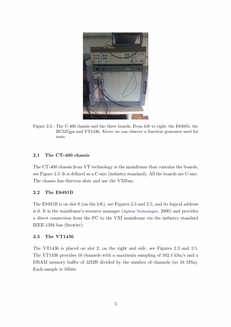
Figure 2.3 - The C-400 chassis and the three boards. From left to right: the E8491b, theBC537gps and VT1436. Above we can observe a function generator used fortests.

2.1 The CT-400 chassis

The CT-400 chassis from VT technology is the mainframe that contains the boards,

see Figure 2.3. It is defined as a C-size (industry standard). All the boards are C-size.

The chassis has thirteen slots and use the VXIbus.

2.2 The E8491B

The E8491B is on slot 0 (on the left), see Figures 2.3 and 2.5, and its logical address

is 0. It is the mainframe’s resource manager (Agilent Technologies, 2006) and provides

a direct connection from the PC to the VXI mainframe via the industry standard

IEEE-1394 bus (firewire).

2.3 The VT1436

The VT1436 is placed on slot 2, on the right and side, see Figures 2.3 and 2.5.

The VT1436 provides 16 channels with a maximum sampling of 102.4 kSa/s and a

DRAM memory buffer of 32MB divided by the number of channels (so 16 MSa).

Each sample is 16bits.

5

2.4 The GPS

The Time Frequency processor (TFP) BC537gps is on slot 1, middle, see Figure 2.3.

It has an internal clock and provides the time with a precision of 0.1 microseconds.

Nevertheless, our precision is not 0.1µs. Accessing the memory of the GPS takes

a few milliseconds. We correct this delay using the PPS. But our precision is then

limited to 1/sampling, see Sections C.8 and D.

The GPS antenna is placed on the building roof. The signal in this case is given by

the GPS, but in case of communication lost, the BC537gps will run in the “flying”

mode. It means using its own clock. Presently, we use the BC537gps to get the

GPS time and the PPS. We use it also to generate a external sampling frequency

synchronized with the pulse per second (PPS) signal. For both functions, we need

to configure the TFP using the GPSmgr program or the SDAQ.

2.5 The Scintillator Veto

Moreover, a scintillator veto was added to the system. This is a veto composed by

three plates and 9 ADC channels. The acquisition of the cosmic rays is independent

of the Mario Schenberg signal acquisition. For the moment these vetoes are going to

be used for offline analysis. A possible adaptation could be done to add a channel to

the real time data acquisition. This is under study. The complete scintillator vetoes

is described in report written by prof. Anderson Fauth of Unicamp (FAUTH, 2011).

2.6 Actual configuration of the VXI instruments

2.6.1 VT1436

Considerations on the clock and sampling frequency:

We can use an internal clock or an external clock that serves as reference for the

sampling. When using the internal clock, the following frequencies [Hz] are available:

40960, 41938.6, 44122.1, 48000, 49152, 50000, 51200, 52400.9, 61440, 62500, 64000,

65536, 66666.6, 76800, 78125, 80000, 81920, 96000, 98304, 100000, 102400

The sampling frequencies are defined as the clock frequencies divided or not by 5

and divided by any multiple of 2. If you program a clock frequency (then a sampling

frequency) that does not match this list above, the VT1436 will use the closest one

on the list.

Remark: For our application, we are interested in the sampling frequency. But the

logic applied inside the VT1436 is not to configure the sampling frequency but the

span frequency. The span frequency is the sampling frequency divided by 2.56. This

6

frequency is in fact currently used in data acquisition. When doing a FFT, the

maximum frequency of our spectra is the sampling frequency divided by two. But

we have artifacts due to the FFT of finite transformation. So dividing by 2.56, we

define a “safer” bandwidth without these artifacts.

To avoid variations of the number of bins per second, we use the external clock, the

clock of the GPS. This problem is described in Section C.1.

The external clock should be within the range of 40960Hz to 102400Hz. Presently,

the given frequency is chosen to match an internal one. This allows us to avoid

radical changes of sampling in case of system failure.

The resonant frequency of Mario Schenberg detector is around 3200Hz. In theory, a

frequency a bit higher than the frequency of our signal (resonant frequency) allows

to reconstruct the signal. Practically, we define a Nyquist frequency as twice as the

minimum required bandwidth, so: 6400Hz. The maximum frequency of FFT space

is:

fmax =sampling

2,

we should use such a sampling that our fmax is above or equal to 6400Hz. But not

too high to generate an excess of useless data.

Frequencies generated by the Time Frequency Processor BC537gps that match

the VT1436 internal frequencies and between the admissible range (40960Hz to

102400Hz) are [Hz]: 57 = 78125, 22 × 56 = 62500, 24 × 55 = 50000, 25 × 55 =

100000, 27 × 54 = 80000.

The second point that we have to take into account is the time resolution dt =

1/(sampling frequency).

Thus we define a set of sampling frequencies (see below) compatible with the defined

criteria, sampling high enough to fulfill the Nyquist condition and a reasonable time

resolution (tens of microseconds) but not too high to generate useless data.

Consideration on others parameters:

The VT1436 allows different acquisition modes.

• The trigger is set to manual. This allows us to control the beginning of the

acquisition.

• The acquisition is set to “continuous mode”. The “block mode” send the

data after each acquisition and wait till it finish sending the data. We lose

7

data in this mode, this problem is shown in Section C.3. The “continuous

mode” continue getting data during the sending process. It keeps data

temporally on the buffer. Thus cuts could appear if we saturate the buffer.

• The transmission to the PC is done per block of data. We have differ-

ent block sizes programed, they are powers of two: 1024, 2048 and 4096

samples. Each sample is 2 bytes. As we will see bellow, we can set in our

program the number of block per file. The function “Repeat ... times” cor-

responds to the numbers of blocks that we save in one file (repeat the block

acquisition).

2.6.2 BC537gps

The TFP could generate a driving clock. This is the “External clock” used by

the VT1436. It is a 10MHz clock. Subdivision frequencies could be obtained do-

ing 10MHz/n1 × n2 where n1 and n2 are two programmable parameters. When we

use the PPS (peak per second) synchronous option, n1 and n2 should be defined

as the desired value minus one unit. For example, to get 100KHz, we set n1 = 1

and n2 = 49 instead of 2 and 50 (Remark: the n2 division is applied first so to get

square signal we should keep n1 = 2). The GPSmgr program allows us to set these

parameters.

In the latest version of the SDAQ, the initialization of the TFP is done automatically.

2.6.3 Parameter summary:

• We program the following list of sampling frequencies [Hz]: 10000, 12500,

15625, 20000. For our measures we will use 15625Hz.

• We use the external clock given by the GPS. This clock is synchronous

with the PPS signal.

• The acquisition is done in continuous mode.

• We have the following block sizes on buffer: 1024, 2048, 4096,

• The size of the file should be of 256 blocks of 1024 (128 of 2048, etc). A

power of 2 optimize the FFT. This number of data corresponds to ∼ 10s.

• The VT1436 channel connections are summarized in the table below. The

PPS is connected at the channel 16.

8

Table 2.1 - Table of correspondences between the position of the transducers on the sphereand the channels used on the DAQ and in the analysis.

Channel Positions on sphere VT1436 channelanalysis φ θ

1 240 79,2 12 120 79,2 23 0 79,2 34 300 37,4 45 180 37,4 96 60 37,4 10

(Notice: To have a determination of the GW arrival, the right orientation of the

sphere should be given respectively to the north).

2.7 How to connect the TFP BC537gps and the VT1436.

The VT1436 entries are SMB connectors also called mini-BNC. The system use SMB

connectors which are not 50Ω terminated.

To connect an external clock, we use the “External Sample SMB” connector on front

panel of the VT1436. The voltage of the external clock signal should be compatible

with the TTL standard (0 to 5V).

On the BC537gps the output connector is a 15-pin connector visible on Figure 2.5.

Both boards are connected trough a 15-pin to SMB adapter cables, see Figure 2.6.

The used pins are:

• Pin 4: PPS

• Pin 15: Periodic Output (the external clock for the VT1436)

• Pin 2 and 12: grounds

The description of pins is defined on Table 6.1 of the BC537gps manual, see Figure

2.4.

9

!"#$%&'()*+

!"# $%!&'()*+$%&',(-./0123/456/7839:35%;/<8=%3>>=8/?@3AB/*C D;223E81%=2/.5%

%,-./(012)345/6(72(,89($.:;(<()=;8,.>

)=;8,.>(?8(72(2@($=8(AB)C )=;8,.>(?8(7<(2@($=8(AB$C$=8 )=;8,. $=8 )=;8,.F G*HE3854I/F,)JK/.5L:E/=8

MA351K36/M>%1II4E=8/M:EL:EF @D"N##/@H?OC

# P8=:56 # @D"N##/@H?"C

& DE8=$3/M:EL:E & @D"N##/0H?OC

N F/<<D/M:EL:E N @D"N##/0H?"C

' 0123/Q=63/M:EL:E/?R)C ' P8=:56

! *HE3854I/*A35E/.5L:E ! S=E/T>36

U 0123/Q=63/.5L:E U P<D/F<<D

V 0123/Q=63/@3E:85 V P<D/@D"N##/F<<DO

W M>%1II4E=8/Q=5E8=I/M:EL:E W P<D/@D"N##/F<<D"

F, S=E/T>36 F, P8=:56

FF 0123/Q=63/M:EL:E/?XQYDC FF P<D/@D"N##/0H?"C

F# P8=:56 F# P<D/@D"N##/0H?OC

F& FZ'ZF,/)JK/M:EL:E F& S=E/T>36

FN *HE3854I/F<<D/.5L:E FN P8=:56

F' <381=61%>/M:EL:E F' P<D/OF#/(XQ

G//<15/F/1>/45/=:EL:E/[\35/E\3/=LE1=54I/=A351K36/=>%1II4E=8/1>/15>E4II36B

Figure 2.4 - Extract of the BC537gps manual.

Figure 2.5 - Close view of the three boards. In the middle, on the BC537gps, we can seethe 15-pin connector (still free). Above we have the connector and cable ofthe GPS antenna.

10

Figure 2.6 - Cable adaptation: 15-pin to SMB.

11

3 MINIMAL INSTALLATION FOR THE DATA ACQUISITION AND

ANALYSIS

3.1 The data acquisition PC: schenbi-daq

The Optiplex 780 runs Windows 7 (64 bits). The hardware configuration is in Annex

A.1.1. This PC is dedicated to run the SDAQ program and in background it monitors

the no-break system from “APC”.

• The connection with the VXI mainframe is done trough the Firewire port.

This port was added with a PCI card. This is a 5V card and has no proper

power supply. Thus we have to connect it in parallel to the floppy disk

power supply cable. A special connector was made for this purpose.

• This PC also monitors the no-break status. It uses a program given by

APC. In case of electricity cut, the no-break has a battery that last a few

hours. After this delay the system is shut down. The APC was programed

to send warning e-mails in case of electricity cut, low battery and other

situations.

The following programs are installed on the DAQ PC :

• Matlab R2009 which runs the SDAQ program. Presently, we are using an

USP license. All the installation indications are available online USP/CCE.

The following tool package are used:

Data acquisition, Statistics, Curve fitting, Control system and Signal pro-

cessing.

• Codeblocks, this is a free C++ compiler, it serves to compile the GPSmgr

program. We use wxWidget to create the GUI. Both could be get free from

the Internet. We need to install a GCC compiler.

• Cygwin allows us to use Linux applications. When installing Cygwin, one

should install the “ssh” tools that allow our remote connections.

• “PowerChute Business Edition” is the APC management program. A

description is available in Annex B.2.

The SDAQ program and GPSmgr need the following drivers:

13

• IOlibrary suite from Agilent (v16.1 64bits, for windows 7). It installs the

application “Agilent Connection Expert.exe”. This last program allows us

to manage the connection to the boards. The IOlibrary suite installation

also includes the VISA libraries which are the interface between the code

machine and the programming code. More indications about the Agilent

program could be found in (COSTA, 2008; Agilent Technologies, 2006). The

help is located in the VISA file.

• VXIplug&play library (64bits), this is the VT1436 plate driver. We

have an installation file that installs this library“hpe1432 64.dll”and other

things. A copy of the library is directly installed in the path of our SDAQ

application.

• Mex-file: hpe1432.mexw64, this is a library used by Matlab. This li-

brary allows Matlab to use the C functions of the“hpe1432 64.dll” libraries.

This file must be placed in the path of the SDAQ.

• “mwagilentvisa.dll”, this library is installed in

C:\Program Files\MATLAB\R2009a\toolbox\instrument\instrumentadaptors.

Our MATLAB program uses it to send commands to the TFP. This is the

VISA interface. This library comes with the version R2010a or superior

versions of Matlab.

The installations files are stored in C:\DAQ \Drivers new

3.2 The server: schenbi-s

The Dell PowerEdge 1900 runs openSUSE 11.4 (64 bits). The hardware configuration

is in Annex A.1.2. This PC is used for real time analysis. It also serves as the interface

between the DAQ PC and Internet.

The Sever needs the following programs :

• Root, the data analysis application from CERN.

The data analysis programs need the following libraries:

• GSL libraries

14

• mG Libraries

• mS Libraries

• Frame Libraries from Ligo-Virgo

• Wavelet Analysis Tool

15

4 SDAQ UTILISATION

Figure 4.1 - Front panel of the SDAQ9 program.

The DAQ system program is written with MATLAB. MATLAB is compatible with

C++ and allows to create graphical interface (GUIDE, see (MATHWORKS, 2002)).

In Figure 4.1 is shown the front panel of the SDAQ program.

The SDAQ9.m could be found in C\DAQ\SDAQprg\SDAQ64\).

The program is divided in five sections. They are described in the order by which

they should be used. The buttons are automatically enabled or disabled when they

can be used or not. To follow the description below, please, refer to Figure 4.1.

4.1 Session management

The first section is the Session management. You will be asked to initiate the

session. No controls are allowed before it.

a) Initiate Session: when pressing this button the program sets all internal

variables to default values. It also sends the commands to initialize the

17

channels of acquisition. The initialization of the BC537gps is done at the

same time (to control the external clock).

b) Set: this button is used when you have selected the kind of data acquisition

you wish. It sends your data acquisition configuration to the board.

c) Reset: cancels the set function.

4.2 ADC configuration

The ADC configuration section is dedicated to measurement settings. It is com-

posed by:

a) Channels: selection of the measured channels.

b) Sampling rate: we have programmed a list of different samplings, see

2.6.3.

c) Range: of the input voltage (peak to peak).

d) Block size: number of samplings acquired from the VT1436 memory.

4.3 Type

In the Type section you will choose how the data are displayed or saved. You have

the choice between:

a) Spectrum: measures the frequency spectrum of the signal.

b) Oscilloscope: measures the signal (voltage).

c) Record to file: the data are not displayed but directly saved to files. First

you can choose the path where to save files. Then you define the file names.

Three options are available:

– MSdata20101107185446 (see filename convention below, Section 6.1).

– Test20101107185446 (see filename convention below).

– You can create your base name and the files are numerated from 1 to

the maximum measurements allowed.

d) Inf loop: is marked when a continuous data acquisition is wanted. If not,

you can choose the number of acquisition.

18

e) Repeat: it defines the number of block that are stored before write to the

file.

4.4 Status

This section is reserved for status information. When the program is initiated, it

shows the date. If not, an error message will be displayed, the communication be-

tween the PC and the boards, including the Agilent board, should be checked.

During measurements it indicates the actual operation done and when needed the

next operation to be done.

4.5 Acquisition

This is the last section to be done before starting acquisition.

a) Start: this button calls the “VT1436 initMeasure” (VXI Technology, 2010).

which serves to define the group channels (and cancel old ones). At this

level parameters of the data acquisition are transmitted to the VT1436.

When possible, parameters are written to the hardware as soon as they

are received. Sometimes, the parameter cannot be written to the hardware

until starting a measurement. In this case, the value of the parameter

is saved in the RAM of the VT1436B module until the measurement is

started with “VT1436 initMeasure.” Finally, the “triggerMeasure” function

is called and the measurement initiates.

b) Stop: stops the data acquisition.

19

5 GPSmrg UTILISATION

The latest version of SDAQ initiate the BC537gps. Nevertheless, other tests could

be done. The GPSmgr (GPS manager) contains predefined command (bit package)

that are used to set the GPS. The description of the “command package” is available

in (SYMMETRICOM, 2004). The front panel of the program in Figure 5.1 is shown.

Figure 5.1 - Front panel of the GPSmgr program.

5.1 Panel

a) The Menu Bar contains all the commands. They will be listed below.

b) The GPS Time window displays the TFP time and the date. In principle

this time is give by the GPS. The configuration could be change.

c) The UTC shift window displays the number of hour that the TFP time

differ from the UTC time.

d) The Control register window display the last status of the register (The

TFP is controlled by registers written and read by the host).

e) The Ack register (Acknowledge register) window shows if the packet was

received or ready to be sent.

f) The Operation Mode displays operation modes)

g) The Status bar display the status of sent command.

5.2 Time

This menu allows us to enable or disable the TFP time acquisition. It is recom-

mended to disable the time when taking data. We can suspect a slowing in the

communication.

21

5.3 TFP mode (called GPS mode)

a) Set Frequency Clock Mode (TIME SYNC MODE): The TFP could

use different clock (its one clock or external clocks), see the section 1.5 of

the manual (SYMMETRICOM, 2004). We can choose between:

– Time code: this function allows the user to select the format and

modulation types associated with an input timing signal.

– Free Running: the TFP runs at the last known oscillator frequency.

– Real Time Clock Mode: the TFP synchronizes to the onboard real

time clock (RTC) IC, and the major time is also derived from the

clock IC.

– GPS Mode: our GPS receiver is located in one antenna. The internal

clock is controlled by the GPS.

b) Set Position mode: this function is specific of the GPS: If the position

is known and static, then time can be determined by measuring the time

of arrival of a single satellite signal. Each satellite broadcasts information

which allows the GPS to calculate the position. Presently, our position is

fixed and we need only time, so one satellite. Three satellites are needed

to get position and four to determine the position and the time. We can

choose to use 4, 3 or only one satellite. The option automatic switch from

one, three or four satellites in function of the reception. It is better to get

our position from the GPS.

5.4 Settings (could be Time Settings)

When we use the GPS, the date and time are set automatically but in other modes

we have to set them manually.

a) Set UTC shift: UTC (coordinated universal time) refers to the old GMT

(Greenwich Meridian Time). The GPS gives the UTC time. We can set the

TFP to display and record our local time by giving the shift hours of the

local position. Remark: When taking scientific data, it is recommended

to use the UTC time so UTC shift 0.

b) Set year: We should set the year if we are not using the GPS.

c) Set Time: the same as above.

22

d) Set GPS or UTC time. The TFP could give the the UTC time (GMT,

date and time) or the number of seconds since 6 January 1980.

5.5 Others Packets

a) “C” Command input: This packet sets machine parameters. As an ex-

ample, we can do a “Software Reset”.

b) “D”Load D/A converter: The TFP reference crystal oscillator is voltage

controlled using the buffered output of a 16 bits D/A converter as the

controlling voltage.

c) “F”Heartbeat control: This packet establishes the frequency of the TFP

output periodic. This is the mode to generate the clock used to drive the

VT1436. For more detail, please refer to (SYMMETRICOM, 2004).

d) “G” Propagation Offset control: This mode is used if we have a delay

in the transmission of the time from GPS to the TFP.

e) “I” Clock Source select: The 10Mhz frequency of the TFP could be

driven from the internal or an external clock.

f) Send packet: Allows you to send any undefined packet.

5.6 Resets

We can reset the receiver (GPS) or the TFP.

a) Reset TFP/Board

b) Reset Receiver

5.7 Status

It prints in a separate windows the TFP configuration and a list of errors.

23

6 FILE STRUCTURE CONVECTION

Files generated by the SDAQ.m program are defined by the following conventions.

Each file contains an header and data are save as floats.

6.1 File names:

The name of the file is defined in the following way:

• The file starts with:

- MSdata when the data are scientific data.

- Test when data belong to tests.

- A name could be specify for special tests.

• When using the MSdata or Test conventions, the name of the file contains

automatically the date in the following format: MSdata20101107185446

- 4 digits for the year

- 2 digits for the month

- 2 digits for the day

- 2 digits for the hour (UTC)

- 2 digits for minutes

- 2 digits for seconds

6.2 File header

The header has the following format:

Total number of bytes 1 byte (Including this byte)

Program version 1-byte

Header version 1-byte

Date of GPS (seconds) 4-bytes

Date of GPS (fraction of seconds) 4-bytes

Date of the file begin (seconds) 4-bytes

Date of the file begin (fraction of seconds) 4-bytes

Number of blocks 2-bytes, unsigned integer type

Size of a block 2-bytes, unsigned integer type

Number of channels 1-byte, unsigned integer type

Sample rate 4-bytes, single

Range 1 byte, unsigned integer type

25

The header format will change according to the evolution of our data. The evolution

is show in the table 6.1.

Table 6.1 - Evolution of the header.

Versionsof program: of header: changes applied:

1-7 n/d - No changes.8 1 - Program version and header

version were added.9 2 - UTC Time was changed

to GPS Time.

6.2.1 Notice about time definitions!

The GPS works with the UTC time or with seconds since 6 January 1980. The date

is given until 10−7s. In the UTC convention, the time was given in the following

format8 bits empty

4 bits for the status

12 bits day of the year (4 bits per day)

8 bits for hours (4 per digit)

8 bits for minutes (4 per digit)

8 bits for seconds (4 per digit)

28 bits for the fraction of seconds (4 per digit till 10−7s)

4 bits empty

The time was saved in this format until the version 9 of the program SDAQ. In

version 9, we opted for the number seconds since 6 January 1980. There are two

reasons for that. First it is more simple to handle and to do time corrections. Second,

this is also the format used in the “Frame” defined by Ligo-Virgo. If we exchange

data with them, we will already have the same format and reference.

Remark: now the time displayed on the GPS card is the GPS time which has 15s

in advance respectively to UTC time.

The UTC time presents corrections of seconds called leap seconds 1. At certain dates,

seconds are subtract to keep the UTC time synchronous with solar time (one second

1see http://en.wikipedia.org/wiki/Leap second

26

each date). These corrections do not allow a simple conversion from UTC time to the

number of seconds from a defined epoch. It is easier to apply the opposite conversion.

6.2.2 Configuration of GPS time (number of seconds)

To read this time the function “init gps.m” was changed to “init gps 2.m” which

include a new packet to send:

“gps send packet(vv,‘PA0’); to Use GPS Time format”

“gps send packet(vv,‘M+00’); to Set time zone, GMT”

At the same time when defining the GPS time, we have to select the option: “ignore

leap second” bit 3=1, see (SYMMETRICOM, 2004) Section 4.1.14. This gives a GPS

time including all the seconds since 6 January 1980.

27

REFERENCES

Agilent Technologies. Agilent e8491b ieee-1394 pc link to vxi, c-size data sheet.

User’s manual, 2006. 3, 5, 14, 53

AGUIAR, O. D.; ANDRADE, L. A.; BARROSO, J. J. et al. The brazilian

gravitational wave detector mario schenberg: status report. Class. Quantum

Grav., v. 23, p. S239–S244, 2006. 1

COSTA, C. A. Sistem de aquisicao de dados do derector de ondas gravitacionais

mario schenberg. Relatorio Tecnico USP, February 2008. 4, 14, 53, 65

COSTA, C. A.; AGUIAR, O. D.; MAGALHAES, N. S. The mario schenberg

gravitational wave detector: A mathematical model for its quadrupolar oscilations.

arXiv:gr-qc/0312035v1, 2003. 1

FAUTH, A. C. Veto de raios cosmicos da antena gravitacional mario schenberg.

Unicamp Internal publication, Sep. 2011. 6

JOHNSON, W. W.; MERKOWITZ, S. M. Truncated icosahedral gravitational

wave antenna. Phys. Rev. Lett., v. 70, n. 16, p. 2367–2370, 1993. 1

MAGGIORE, M. Gravitational Waves, Vol. 1 Theory And Experiments. Oxford

University Press., 2008. 1

MATHWORKS. Matlab help files. Cambridge MA, 2002. 17

MERKOWITZ, S. M.; JOHNSON, W. W. Techniques for detecting gravitational

waves with a spherical antenna. Phys. Rev. D, v. 56, n. 12, p. 7513–7528, 1997. 1

PIMENTEL O D AGUIAR, J. J. B. G. L.; TOBAR, M. E. Investigation of

ultra-high sensitivity klystron cavity transducers for broadband resonant-mass

gravitational wave detectors. In: SCIENCE, I. (Ed.). J. Phys.: Conf. Ser. [S.l.:

s.n.], 2008. v. 122, n. 012028. 1

SYMMETRICOM. bc637VME/bc357VXI GPS Satellite Receiver Addendum.

Online: www.symmetricom.com. 65

. bc635VME/bc350VXI Time and Frequency Processor. Online:

www.symmetricom.com, January 2004. 3, 21, 22, 23, 27, 65

VXI Technology. Vt1432b 4-/8-/16-channel, 102.4 ksa/s digitizer plus dsp. User’s

manual, July 2010. 3, 19, 69, 70

29

ZHOU, C. Z.; MICHELSON, P. F. Spherical resonant-mass gravitational wave

detectors. Phys. Rev. D, American Physical Society, v. 51, p. 2517–2545, Mar

1995. 1

30

APPENDIX A- PC CONFIGURATION AND INSTALLATIONS

A.1 Hardware

A.1.1 DAQ PC, shenbi-daq

This is an Dell OptiPlex 780.

• Processador Intel¨ CoreT2 Quad Q9650 (3.00GHZ, 12M, 1333MHZ FSB)

• RAM 16GB

• HD 500GB SATA, 7200RPM

• 2× HD 2TB SATA

• DVD 16X DVD+/-RW SATA

• Warranty: “4 anos de Garantia Pro Support com atendimento telefonico

24x7”, TAG 50TJNQ1

Presently, it is running Windows7 professional.

A.1.2 Server, shenbi-s

The server is a DELL computer “PowerEdge 1900”.

• Two Dual-Core Intel Xeon Processors 5000

• RAM 16GB

• 4 HD of 250G mounted in RAID 5

• DVD 16X DVD+/-RW SATA

• Various PCI (one full-height, half-length 3.3-V, 64-bit, 133-MHz (slot 1);

one full-height, full-length 3.3-V, 64-bit, 133-MHz (slot 2); one x8 lane,

3.3-V (slot 3); three x4 lanes, 3.3-V (slots 4 through 6).

• Warranty: TAG 9T7FMC1

31

More informations about the hardware could be obtain in the terminal using the

command: hwinfo –short.

Presently, it is running openSuse 11.4. In parallel we keep an installation of windows

2008. This version is not supported yet by the IOlibraries. Then this system could

not be used for the DAQ.

A.1.3 Hard disks

Our system uses HD installed in RAID (Redundant Array of Independent Drives).

HD manipulations should be cared.

We use the following configuration:

- schenbi-daq:

We installed internally one disk of 500GB and 4TB (2 disks of 2TB each,

mounted in one logical volume). Externally, we keep a copy of the data in

“schenbi-data 1” a logical volume of 4TB (2 samsung disks mounted in one

case MTEK). The HD extern is connected with via e-SATA.

Attention: there is no plug&play function for the e-SATA. So always shut

down the PC before unmount the disk.

- schenbi-s:

We have internally 4disks of 250GB (mounted in RAID 5). Our total mem-

ory is 860GB, due to RAID5 mirroring we loose 25%. Externally, we have

a Iomega case with 2 disks of 2TB each mounted in RAID 1 (“schenbi-

data 2” and “schenbi-data 3”). We have then a copy of the analyzed data

in each disk. The Iomega is connected via e-sata.

Details on the RAID:

“It is a technology that provides increased storage functions and reliability through

redundancy. This is achieved by combining multiple disk drive components into a

logical unit, where data is distributed across the drives in one of several ways called

RAID levels.” (Wikipedia)

“RAID 0 (block-level striping without parity or mirroring) has no (or zero) redun-

dancy. It provides improved performance and additional storage but no fault toler-

ance. Hence simple stripe sets are normally referred to as RAID 0. Data written to

a RAID 0 volume are broken into fragments called blocks. Blocks are written in par-

allel to different disks. Any drive failure destroys the array, and the likelihood

32

of failure increases with more drives in the array (at a minimum, catastrophic data

loss is almost twice as likely compared to single drives without RAID).” (Wikipedia)

“RAID 1 (mirroring without parity or striping), data is written identically to multiple

drives.” (Wikipedia)

“RAID 5 is a cluster-level implementation of data with “distributed parity or mir-

roring”. Clusters can vary in size and are user-definable but they are typically blocks

of 64 thousand bytes. The clusters and parity are evenly distributed across multiple

hard drives, as shown in Figure A.1 and this provides better performance than us-

ing a single drive for parity. Out of an array with ONO number of drives, the total

capacity is equal to the sum of ON-1? hard drives. For example, an array with 4

equal sized hard drives will have the combined capacity of 3 hard drives. This is the

most common implementation of data striping with parity. In this example 25% of

the storage purchased is used for duplication (internet sources).” (Wikipedia)

Never unmount two disk at the same time! We get problems with it. It corrupts

the disks. In raid 5, a copy of the missing part is done in remanning disks. So if two

disk fail at the same time, the raid 5 could not managed it.

Figure A.1 - Schema of the RAID 5 parity.

Configuration of the RAID on the Iomega case

Behind the Iomega HD, are located two switches. Four different configurations are

possible. We can pass from an extended logical disk, RAID 0 and RAID1, see the

manual. RAID1 is mirroring of the two disks. In this case we have only 2TB.

33

Configuration of the RAID on the server

The raid could be configured during the BIOS initialization. At a certain moment you

will be call to change RAID pressing the CTRL+R command. You will enter in the

RAID configuration. The are 3 pages. The first pages presents you the configuration

(we have only one ”configuration 0”). If you press F2 when this configuration is

selected you will reset it and creates a new one.

A.2 Internet and ethernet connections.

The two PCs (Server and DAQ PC) are connected via ethernet. They use two

gigabit cards. The server has another gigabit connexion for Internet.

Their DNS and names were set as:

• DAQ PC: schenbi-daq

• Server: shenbi-s

A.2.1 schenbi-daq

This computer should perform the following tasks:

• Connect to the server.

• Access internet (port 80).

• Send email alerts.

• Allows ssh connections (“ssh” which was installed with Cygwin, port 22).

• It should access the Licence server of the USP (for MATLAB).

• We want to have a Remote Desktop access (port 3389).

For this purpose it is configured as follow:

First, we assign it the IP 192.168.1.2 and as a gateway the IP of the server 192.168.1.1

see Figure A.2. We do not give the DNS to avoid direct connection with the exterior.

34

Figure A.2 - schenbi-daq IP configuration

Figure A.3 - Configuration to use a proxy. (Proxy defined in the server.)

To connect to the Internet, we use a proxy, see Figure A.3.

Finally, we use a Firewall to protect the USP net, see Figure A.4. If the the DAQ

computer is contaminated by a virus it could not spread its virus. In the opposite

way, it is itself protected by the server firewall.

35

Figure A.4 - Configuration of the Firewall. We authorize only connections to the server(192.168.1.1 or the Licence server of the USP 200.144.188.41.

36

A.2.2 schenbi-s

This computer should perform the following tasks:

• Connect to the DAQ PC

• Access internet (port 80) and serves as proxy for the DAQ PC.

• Forward the DAQ emails (It use a mail server “postfix”, see below.).

• Allows ssh connections (port 22).

Remarks: The port 22 is open by USP on our demand. If it fails one

should ask the USP CCE service.

• It allows VNC connections.

• It make an IP maskering for Remote Desktop (port 3389).

• We close the firewall except for the application above.

Most of the command panel for the configuration are in the Yast2 manager.

First lets configure the IP, gateway and DNS, see Figures A.5, A.6 and A.7.

37

Figure A.5 - To avoid configuration problems, we use the “ifup” method. The Network-Manager does not recognize one plate.

38

Figure A.6 - We set the internal IP (eth0) as 192.168.1.1 and the external as 143.107.133.6(eth1). As we can see the server name is schenbi-s. For the external IP, weconfigure the usual DNS of the USP.

39

Figure A.7 - The Gateway (or router) is 143.107.133.1

40

Then we set the firewall and the maskering for Remote Desktop connections, see

Figures A.8 and A.9:

Figure A.8 - We should enable the service to get the maskering. The firewall has twoconfigurations. For internal connection (between the two PC’s), we apply nospecial rules. For external connections, we allow only a few programs, seebelow.

41

Figure A.9 - We allows access with “ssh” (port 22), VNC (port 5901, websharing VNC143.107.133.6:5801. We apply a masquerade (or port forwarding) for Re-mote Desktop (3389). All accesses on this port are redirected to schenbi-daq192.168.1.1.

42

Finally, we enable VNC connections in Remote administration, see Figure A.10

Figure A.10 - The exception of VNC is automatically added in the firewall.

43

Configuring the email server

We will use a dedicate gmail account for the project as outgoing mail server. First,search for the mail server in YAST manager. Open it, then we select a standardconfiguration, see Figure A.11.

Figure A.11 - Views of the YAST manager and the Server mail configuration.

44

We select the permanent connection, see Figure A.12 and enter the smpt server ofgmail (smpt.gmail.com port 587).

Figure A.12 - Views of the YAST manager: general settings and outgoing mail server set-tings.

45

We define a masquerade, the user “schenberg” will be define by the email“schenbi.m@gmail.com”. This is not compulsory. For connections to gmail server,we will use authentication method (user, password), see Figure A.13.

Figure A.13 - Views of the YAST manager and the Server mail configuration (2).

46

The incoming email is not useful except for mails received from the daq pc (schenbi-daq). We need only to open the port in the firewall from the schenbi-daq, see FigureA.14. Schenbi-daq is connected to the ethernet board 0.

Figure A.14 - Views of the YAST manager and the Server mail configuration.

At this level all mails receive from schenbi-daq are sent trough the gmail account.

47

APPENDIX B- APPLICATIONS USED BY DAQ PC

B.1 Cygwin

Cygwin emulates a UNIX environment. We can use all the tools of UNIX including

“ssh”.

B.1.1 How to install it:

• Download Cygwin from internet.

• Follow the setup. Install the following packages:

Net: choose all the applications related to ssh, ftp and tunneling.

Editors: vi, emacs

shell: all the bash

Documenting:

Install gcc

• When installed, start the application Cygwin. A terminal will open. Launch

it as an administrator.

• Now we will configure openSSH.

B.1.2 How to configure SSH

0 The read-me is in: usr/share/doc/.

1 In usr/bin: configure the openssh.readme

2 Then execute the ssh-host-config (you need to start Cygwin as admin, right

click on Windows OS)

3 Basically check yes all options.

4 Set ssh-user-config, choose a simple user name. We choose the same as

windows.

5 To finish launch the openssh: net start sshd

49

B.2 How to use APC program

The APC no-break is connected to the schenbi-daq pc. A special cable USB- RJ45

make the connection between the APC and the PC.

The APC no-break comes with two installation CDs containing 3 applications. You

should install: “PowerChute Business Edition”. The server is used only when many

PC are connected to different APC systems.

The monitoring application is a web interface application (User Schenberg, password

see list of passwords). The program is located in:

C:\Users\Schenberg\AppData\Roaming\Microsoft\Windows\Start

Menu\Programs. Or you could start it from the browser: https://schenbi-

daq:6547/main and from the start menu: “APC PowerShut Business Agent/Agent

web Interface”. Remark: it does not work with Mozilla, you should use Explorer.

It could send mails or execute specific scripts. The command scripts are in a reserved

repertory. Presently we use only the email function. The program is configured

with an email dedicated to the detector Schenberg (schenbi.m@gmail.com) and the

smtp server is the schenbi-s pc (192.168.1.1), see below. The server is configured as

a mail server, see the schenbi-s configuration.

Remark: To add a new script the easiest way is to modify an existing one and to

save it with a new name. An example could be already found in the dedicate file:

c:\Programs (x86)\APC\PowerChuteBusiness\agent\cmdfiles.

B.2.1 To configure the APC

First step, open the program: “APC PowerChute Business Edition Deluxe”, see Fig-

ure B.1.

50

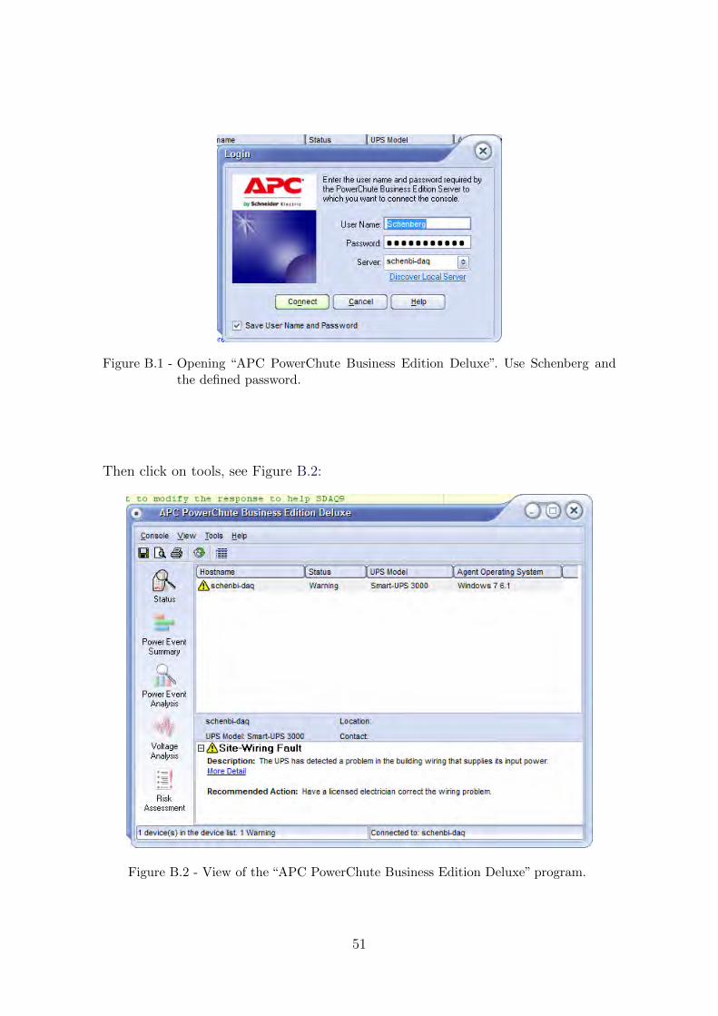
Figure B.1 - Opening “APC PowerChute Business Edition Deluxe”. Use Schenberg andthe defined password.

Then click on tools, see Figure B.2:

Figure B.2 - View of the “APC PowerChute Business Edition Deluxe” program.

51

Configure the smtp server, see Figure B.3 and click in SMTP settings, see Figure B.4.

Figure B.3 - SMTP configuration of the APC.

Figure B.4 - SMTP configuration of the APC.

52

B.3 C++ compiler

We have installed an open source compiler: Codeblocks. It installs with it the mingw

”Minimal GNU for Windows” which contains a gcc. There is no special setup.

Then we have installed a library wxWidgets.org (wxMSW - installer for Windows,

with manual (other formats: zip)) to implement GUI (visual interface).

Once installed, we will found the following repertory: build/msw/config.gcc. We

should add gcc to the path (command prompt): PATH=%PATH%; Next command:

mingw32-make -f makefile.gcc

That’s all folks!

B.4 Drivers 32bit

The DAQ PC could run a 32bits version of our DAQ (the server could also run

the system in 32bits using the windows system “server 2003 service pack 2”). The

configuration is almost the same as for 64bits.

• The IOlibrary suite from Agilent (v15): This suit install the application

Agilent Connection Expert.exe. This last programs allows us to manage

the connection to the boards. The IOlibrary suite installation includes the

VISA libraries which are the interface between the code machine and the

programming code. More indications about the Agilent program could be

found in (COSTA, 2008; Agilent Technologies, 2006). The help is located in

the VISA file.

• The VXIplug&play library: It installs the vt1432.dll1 library that could

be used with Matlab and C programs. The help is in the VXIpnp file.

• The Mex-file, this is a library used by Matlab. This library allows us to

use the C vt1432 libraries. This file must be place in the path of your

Matlab application. The Library is called: ”vt432.dll”, in future version the

mex file will not have the same name as the library.

• We also need the: ”mwagilentvisa.dll” which is included in the toolbox of

Matlab. This library contains functions used to control the GPS.

1The name vt1432 is misleading, in fact this is the driver for the plate versions 1432-36, notonly 1432.

53

APPENDIX C- TESTS OF THE DAQ

All the data of the tests described below are stored in schenbi-daq:

C\DAQ\TestsDAQ.

C.1 External clock tension

The tension of the TFP periodic signal (used for the sampling) should be TTL

compatible. It means at least 3V, preferably 5V. The measured tension is ∼ 4V, see

Figure C.1.

0 500 1000 1500 2000 2500−0.5

0

0.5

1

1.5

2

2.5

3

3.5

4

4.5

Vol

ts

Sample Number

T1

Figure C.1 - Voltage of the TFP periodic signal. The number of bins is not relevant forthis measure.

C.2 TFP periodic signal and PPS synchronization

The TFP BC357GPS generate a signal that could be synchronous or asynchronous

with the PPS. We want it to be synchronous to have a complete control on the

number of bins in a second. In asynchronous mode, the two signals start at different

times, as shown in Figure C.2. So we will not have a bin starting exactly at the

beginning of the of the PPS.

55

7000 7500 8000 8500 9000 9500 10000−0.5

0

0.5

1

1.5

2

2.5

3

3.5

4

4.5

Vol

ts

Sample Number

X: 8123Y: 0.05113

T1T2

Figure C.2 - The PPS signal is the green line (long peak, T2). The periodic signal is theblue line (shorter peaks, T1). The frequency used for the test is 25Hz. Remark:one peak is cut. This is due to the “block mode” of the acquisition.

In Figure C.3, we see the case when the BC357GPS is in mode synchronous. The

two peaks are perfectly synchronized. The two rising edges are in coincidence.

1.05 1.055 1.06 1.065 1.07 1.075 1.08 1.085 1.09 1.095 1.1

x 104

−0.5

0

0.5

1

1.5

2

2.5

3

3.5

4

4.5

Vol

ts

Sample Number

T1T2

Figure C.3 - The PPS signal is the green line (long peak, T2). The periodic signal is theblue line (shorter peak, T1). The frequency used for the test is 25Hz.

56

C.3 Block mode

In Figure C.4 is shown the effect of the acquisition “block mode”. When the system

is in block mode, it waits until the data are sent before continuing the acquisition.

For this reason, we use only continuos mode. The option block mode was suppressed

from the SDAQ program.

1 1.01 1.02 1.03 1.04 1.05 1.06 1.07 1.08 1.09 1.1

x 104

−0.5

−0.4

−0.3

−0.2

−0.1

0

0.1

0.2

0.3

0.4

0.5

Vol

ts

Sample Number

X: 1.024e+004Y: −0.2326

T1

Figure C.4 - Data loss due to the block mode.

We used a signal generator with a sinusoid of 60Hz to check the continuity of our

data acquisition. The sampling is 25600Hz 1.

C.4 Numbers of bins per second.

When using the internal clock we get a shift between the PPS and the internal clock

of the VT1436. The number of bins is not constant, see Figure C.5. This was tested

with 40s of data. Approximately one over two PPS intervals is lower than 25600 bins

(the chosen sampling). The lost bin represents 3.3s per day.

The number of bins was also tested with other sampling frequencies. If the sampling

was higher we loose one or two bins with a frequency of approximately every 6 PPS.

1The parameters of the sinusoid frequency and sampling are not indicated. Nevertheless, theinterest is to show the effect of the loose of data due to the block mode.

57

With a lower frequency we loose less bin.

Figure C.5 - Histogram of PPS time interval. One bin represents 39µs.

We proceed at the same test with the external clock. This clock is synchronous with

the PPS signal. We can choose to synchronize the clock on the rising or lowering

edge of the PPS. Here we tested with the option down. The continuities was tested

for more than 18h (66144s). The sampling was 25000Hz which is more convenient

to set the external clock. We get over 18hours the right number of bin per second,

see Figure C.6.

This test was repeated two more times with the same sampling 25000Hz for 12hours

and the results were the same, see Section C.5.1 for more details. The data are stored

in the files “Test continuity 19 3”, “Sinus 100hz 18 8 11” and “rampa 5s 18 8 11”.

To finish, we also tested another sampling frequency 15600Hz, still using the syn-

chronous mode (but in the up mode). All the PPS intervals have the same binning,

see Figure C.7.

C.5 Continuity of data acquisition

C.5.1 PPS as a continuity test

Actually a simple way to test the continuity of the data is to count the number

of PPS and to check as above if the binning remains constant. It was tested with

the following data: “Sinus 100hz 18 8 11” and “rampa 5s 18 8 11” where we have

58

2.4998 2.4999 2.5 2.5001 2.5002

x 104

0

1

2

3

4

5

6

7x 104

Number of bin

Num

ber

of in

terv

al

Figure C.6 - Histogram of PPS time interval for 18h of tests using the PPS synchroniza-tion.

1.5623 1.5624 1.5625 1.5626 1.5627

x 104

0

10

20

30

40

50

60

70

Figure C.7 - Histogram of PPS time intervals for 65s using the PPS synchronization: clock62500, sampling 15625Hz.

register in canal 1 a specific signal and in canal 16 the PPS.

Both tests have exactly the same amount of PPS which correspond at the number

of seconds of acquisition. The binning remains also constant: 25000bins. This test

shows that in 12h, we do not loose any data.

59

Table C.1 - Number of PPS found across the 2110 files for each test.

Sinus 100hz rampa 5sSampling 25kHz 25kHzBlocksize 1024 1024nb of blocks per file 500 500nb of files 2110 2110seconds 43212,8 43212,8nb of PPS 43213 43213

C.5.2 Phase shift of two sine signals

A way to test the continuity is to measure a sinusoid signal with our DAQ and to

compare it with an ideal signal. The signal was generated by function generator.

We test phase shift difference between the two sinusoids. If the phase shift remains

constant (except normal errors due to the signal) it will indicate no data lost.

First we try to apply this method bin per bin. This test is not suitable for the

following reasons:

• An amplitude variation simulates change in the phase.

• A variation of the injected signal frequency also mimic a phase shift. If the

two frequencies are constant we get a constant ramp, see Picture C.8. The

frequency of the injected signal is not at 1000Hz, it has a difference of:

∆f =| − 1, 341 + 0.786|2π102400/25000

= 0.021Hz

A FFT gives the signal frequency, but to get enough resolution we have

to examine many seconds of data. The limit of the resolution is given by

sampling/(2 ∗ number of data). In the opposite way if we are confront to

quick change in the frequency we have to check small time periods.

• Last point, the method to get the phase shift is not simple and the method

show some artifacts. The large zone in Figure C.8 is due to a few points

between others points that have a jump of phase.

Another option:

We have measured another sinusoidal with a frequency of 100Hz and amplitude 5V

pp. We took 2110 files of 1024 × 500 data each, the equivalent of 12h. We have

60

0 5 10 15 20 25 30 35 40 45−8

−6

−4

−2

0

2

4

Time [S]

Pha

se R

adia

n

Figure C.8 - Phase shift in function of the time.

examined simultaneously the time period, the frequency and the phase of the signal

over many periods.

As we can see in Figure C.9, the number of bins is practically constant. The expected

number was given by the sampling/signal frequency = 25000/100 = 250. We get

4249025× 250bins, 29100× 249bins and 43100× 251bins. The expected number of

periods is number of data/250 = 4321280. The number of periods registered was

4321225. The difference is not due to data lost but to the variations of bins per

period. If we take the number of period with 251 less the number of period with

249, we get 43100− 29100 = 14000bins. This number of bins 14000 corresponds to

56 periods of 250bins, the missing number of periods. We can conclude that we lose

no data.

The variation is due to a slight difference in the frequency of the signal. We perform

a FFT of the signal over 211 files and get a frequency of 99.9986Hz. We can observe

this phase shift by monitoring the first value of each sinus period, the first non zero

value. In Figure C.10, values of 80 periods are shown. Values slightly decrease. It

means that a period 250bins cuts each time a bit earlier the real period. Then the

61

235 240 245 250 255 260 2650

0.5

1

1.5

2

2.5

3

3.5

4

4.5x 106

Bin Count: 4.25e+06

Bin Center: 250Bin Edges: [250, 251]

Bins per period

Num

ber

of b

ins

Figure C.9 - Number of bins per period. The sampling was 25kHz and the signal frequency100Hz.

0 10 20 30 40 50 60 70 80

0.075

0.08

0.085

0.09

0.095

0.1

0.105

0.11

0.115

Tension [V]

Inde

x of

inte

rsec

tion

Figure C.10 - Value of the first bin of 80 periods.

period is slightly higher than 250bins. Actually, if we divide the the number of data

by the number of periods that we get, the period should last 250.003bins. From the

FFT test, the period is 250.0035bins. This confirm our suppositions.

62

Remarks: I have done a few programs that could be used to tests signals. My

programs give the frequency and the phase shift phase of two continuous sinusoids.

The phase is given by the difference of the two complex number phases of the signal

frequency bin.

C.5.3 Test of ramp signal

The main goal of this test is to test the continuity of the data. Actually, if we have

a discontinuity it should happen between blocks. So we have apply a signal with a

slow ramp, a period of 30s. No lost bin was observed.

C.6 Test of the GPS failure

The TFP behavior was tested. We simulated a loss of GPS reception. We take 350

files of 500 blocks. The size of one block is 1024 samples. During the file number 97,

we switched the TFP clock to use the internal clock instead of the GPS. During the

file 230, we switched back the situation. The clock was still synchronous with the

GPS:

- The time of the test: 350× 500× 1024/25000 = 7168

- We found exactly 7168 PPS. All intervals are 25000bins.

The cut last 2867,2s so 47’ 47”. It means that in such laps of time no delay was

registered. We should perform a longer test.

C.7 Test of the SDAQ time performances

To be performed: to check the time that each operation takes including the correction

of the “time of acquisition” .

C.8 Checking the delay of the GPS reading

The header of the files was changed to contain the GPS reading time and the time

of the begin of the file. 7200 files of data were measured, which corresponds to ∼8h

of data. We compare the two times to get the delay that the system takes to read

the time (access the GPS memory), see the algorithm Section D.

It takes: in average 0.012[s] with a standard deviation 0.004[s], see Figure C.11

To confirm that our measure was right and that the correction was also right, we

tested starting times interval for each two consecutive files. Over 7199 intervals,

we get: in average 4.096[s] and standard deviation of 0[s], see Figure C.12. All the

files presents exactly the right starting time. The correction is correct. The used

63

Figure C.11 - Time delays of the GPS reading for 7200 files.

Figure C.12 - Consecutive time intervals between 7200 files.

algorithm is described in section D.

C.9 Electronic delay of the signals

The electronic delay of the circuit should be tested. First the electronic delay of the

veto is computed. Showers of astroparticles will be seen by the detector as events

with hight energy. Then astroparticle event times will serve as a reference to calibrate

the electronic delay of our system. We have to check if this delay is bigger or smaller

than the bin precision of our samplings ∼64µs?

64

APPENDIX D- SYNCHRONISATION OF THE DATA

When acquiring data we register the starting time of acquisition (GPS reading).

This time is saved in the header of the data file. The problem is that this time is

collected with a delay (tested by Cesar Costa, see (COSTA, 2008)). This is due to

the mapping time of the TFP memory.

With our data, we record an extra channel containing the Pulse Per Second signal

(PPS) of the GPS. This channel is synchronised with the data acquisition channels.

To correct our starting time, we use this PPS. The PPS is a rectangular pulse signal

of 200ms, see Figure D.1 and Reference (SYMMETRICOM, 2004). It starts exactly at

full seconds with a precision of 1µs, see (SYMMETRICOM, ).

1 2 3 4 5 6 7 8 9

x 104

−0.5

0

0.5

1

1.5

2

2.5

3

3.5

4

Number of bins

Ten

sion

[V]

Figure D.1 - Shape of the PPS signal. The sampling is 25kHz.

D.1 Algorithm

To know the right starting time of the data we proceed as follow:

• The time of the GPS could be read during an incomplete pulse or before

a complete pulse. It depends only when we start acquiring data.

• We first find the position of the first complete pulse on the data.

65

• We know that this pulse is gave at a complete second.

• Then we compute, knowing the number of bin to the beginning of the file,

the time before this pulse: nb of Bin/sampling.

• To finish we cross check the information of the GPS and the position of

the pulse to find the real starting time of the file.

• We can have two cases:

1) If the time to the beginning is less than one second. In this case we just

change the fraction of the seconds that the GPS gave.

2) If the time to the beginning is negative, it means that we are considering

the wrong second as reference, we have to subtract 1s to the GPS second.

It happens when the PPS starts just before the GPS time reading.

To find the pulse we use the following parameters of the PPS. As we can see in

Figure D.2, the distribution of the tension is clearly separated between the low level

(0.5V) and the high level (4V).

−2 −1 0 1 2 3 4 5 60

5

10

15x 106

Tension [V]

Num

ber

of b

ins

Figure D.2 - Histogram of the PPS tension. We see clearly two peaks corresponding to thelow and hight state of the pulse. The average vales are 0,5V for the low stateand 4V for the high state.

The rising edge of the of the PPS is sharp, only 1 to 3 points, see Figure D.3.

66

29.39 29.3905 29.391 29.3915−0.5

0

0.5

1

1.5

2

2.5

3

3.5

4

X: 29.39Y: 1.769

Time [s]

Ten

sion

[V]

Figure D.3 - Close view of the rising edge of one PPS signal. This edge has only one pointin the middle.

Then our algorithm search only for the rising edge. We test two points, if the first

point is below and the second above a fix threshold of 3.5V. This simple test guar-

antees us to select the rising edge. We select always the second point.

Remark:To spare some computing time we do not test the points of the high voltage.

Once we find the edge we skip the following point (number of bins equivalent to

0.19s).

As example program: “Test correction GPS time” is located in:

C\DAQ\SDAQprg\Examples\.

67

APPENDIX E- CHANGING THE SDAQ PROGRAM

“The VXIplug&play Library “hpe1432.dll” communicates with the hardware using

VISA (Virtual Instrument Software Architecture). VISA is the input/output stan-

dard upon which all the VXIplug&play software components are based” (VXI Tech-

nology, 2010).

The SDAQ, in MATLAB, uses the MEX file hpe1432.mexw64 as interface to use the

library “hpe1432.dll”. This file must be placed in the same directory as the SDAQ.

E.1 VXI boards logical addresses (LA):

To send commands to the boards we need to access them by their logical addresses.

The logical addresses could be find using the Agilent Connection Expert program.

Presently we have the following configuration:

• Agilent E8491B: slot 0: LA 0

• Symetricom BC537gps: slot 1: LA 253

• VXITech VT1436: slot 2: LA 8

E.2 Functions

In MATLAB all functions have the same structures (in the version 64bit their name

start by “hpe” and in 32bit it is “vt”):

[status] = hpe1432(’deleteAllChanGroups’,session);

They are overloads of the same function hpe1432(). The function is defined by the

string which specify the action of the function. So each function returns and gets as

entries one or more parameters in function of the defined action.

E.3 List of functions

This list is not exhaustive:

• hpe1432(‘find’)

“This function searches the VXI mainframe and returns the VXI Logical

Address for every VT1432B found.”

• hpe1432(’getHWConfig’)

“This function returns additional information about the hardware.”

69

• [config.status, config.session ]= hpe1432(’init’,’VXI0::8::INSTR’,1,1);

“This function initializes the VXIplug&play library and registers all

VT1432B modules. It also checks the existence of a VT1432B module

at each of the logical addresses given in the resource list and allocates

logical channel identifiers for each channel in all of the VT1432Bs. Input

channels, source channels, and tachometer/trigger channels are kept

logically separated. (VXI Technology, 2010)” The two function before could

be used before ’init’.

• hpe1432(’getNumChans’)

This function get the total count of inputs, sources, and tachs for all

VT1432B modules named in the hpe1432(’init’) call.

• [status] = hpe1432(’deleteAllChanGroups’,session);

This function delete the groups of channel. It used before the creation of

groups to ensure that no group exist before creating one. Conflicts may

appear if this precaution is not taken.

• [status,gid] = hpe1432(’createChannelGroup’,session,length(OLDCHANNELS),OLDCHANNELS);

To control a channel, this channel must be included in a group. A channel

group is unite base for the VXI.

• [status] = hpe1432(’setActive’,session,gid,’CHANNEL_OFF’);

When deleting a group, some channels could remain active saturating the

buffer. Channels must be explicitly deactivated before deleting the group.

This is done withe the ’setActive’ command.

• vt1432_check_status(session, status);

This is function actually is a function wrote in MATLAB which calls two

functions from the library. The file “vt1432 check status.m” should be ex-

plicitly in the MATLAB repertory. The two functions are ’error message’

and ’errorDetails’. It is recommended to check the status after all com-

mands. The status is a return value of all functions.

• [status] = hpe1432(’setBlocksize’,session,gid,BLOCKSIZE);

The block size is the number of sample points in a block of data. All the

active channels have the same block size.

• [status, actual_blocksize] = hpe1432(’getBlocksize’,session,gid);

Get the block size of all active channels.

70

• [status] = hpe1432(’setRange’,session,gid,RANGE);

Set the full scale voltage range of all active channels.

• [status, actual_range] = hpe1432(’getRange’,session,gid);

Get the full scale voltage range of all active.

channels.

• [status] = hpe1432(’setSpan’,session,gid,SPAN);

The rate at which the measurement data is sampled. For the VT1432B,

the sample rate is 2.56 times the frequency span (2.56 × span= sample

rate) . Sample rate is abbreviated OfsO (for Osample frequencyO).

• [status, actual_span] = hpe1432(’getSpan’,session,gid);

Get the SPAN (sample rate/2.56).

• [status] = hpe1432(’setDataMode’,session,gid,’BLOCK_MODE’);

Put module in block acquisition mode. “In block mode, the input hardware

acquires one block after getting an arm and trigger. It does not allow the

system to trigger until it is ready to process the trigger and it acquires

pre-trigger data if necessary. The hardware does not accept a new arm and

trigger until the acquired block is sent to the host. There is no provision

for overlap or queuing up more than one block when in block mode. There

is also no way for a FIFO overflow to occur.”

• [status] = hpe1432(’setAutoTrigger’,session,gid,’MANUAL_TRIG-

GER’);

Set the trigger mode. They are 8 trigger modes. “Triggering is defined as

the transition from the ARMED state to the TRIGGER state.”

• [status] = hpe1432(’initMeasure’,session,gid);

Start measurement.

71

APPENDIX F- CHANGING THE BC537GPS PROGRAM

F.1 List of functions

The new version is written with“Codeblocks”and the GUI is done using the wxWid-

get libraries.

All the function to communicated with the TFP board are in the files “sym lib.h”

and “.cpp”. It use the VISA functions. The program is written in c++.

We can give just as an example the two basic function ton sen and get bytes.

• To send:

void poke( ViSession seg, ViAddr off, unsigned short word )

viPoke16( seg, off, word ); \\ VISA function see the VISA help.

return;

• To receive:

unsigned short peek( ViSession seg, ViAddr off )

unsigned short word;

viPeek16( seg, off, & word ); \\ VISA function see the VISA help.

return word;

73

APPENDIX G- COMMUNICATION BETWEEN THE SDAQ AND

THE LOW LATENCY ANALYSIS

The basic code is the following:

com=tcpip(192.168.1.1, 4000); (IP and port)

fopen(com);

fwrite(com, ‘A’);

fprintf(com, ‘texto...’) fclose(com):

For more help, see the MATLAB function “tcpip” and example other examples are

available at:

http://www.mathworks.com/products/instrument/hardware/tcpip.html

75

PUBLICACOES TECNICO-CIENTIFICAS EDITADAS PELO INPE

Teses e Dissertacoes (TDI) Manuais Tecnicos (MAN)

Teses e Dissertacoes apresentadas nosCursos de Pos-Graduacao do INPE.

Sao publicacoes de carater tecnico queincluem normas, procedimentos, in-strucoes e orientacoes.

Notas Tecnico-Cientıficas (NTC) Relatorios de Pesquisa (RPQ)

Incluem resultados preliminares depesquisa, descricao de equipamentos,descricao e ou documentacao de progra-mas de computador, descricao de sis-temas e experimentos, apresentacao detestes, dados, atlas, e documentacao deprojetos de engenharia.

Reportam resultados ou progressos depesquisas tanto de natureza tecnicaquanto cientıfica, cujo nıvel seja com-patıvel com o de uma publicacao emperiodico nacional ou internacional.

Propostas e Relatorios de Projetos(PRP)

Publicacoes Didaticas (PUD)

Sao propostas de projetos tecnico-cientıficos e relatorios de acompan-hamento de projetos, atividades e con-venios.

Incluem apostilas, notas de aula e man-uais didaticos.

Publicacoes Seriadas Programas de Computador (PDC)

Sao os seriados tecnico-cientıficos: bo-letins, periodicos, anuarios e anais deeventos (simposios e congressos). Con-stam destas publicacoes o InternacionalStandard Serial Number (ISSN), que eum codigo unico e definitivo para iden-tificacao de tıtulos de seriados.

Sao a sequencia de instrucoes ou codi-gos, expressos em uma linguagem deprogramacao compilada ou interpre-tada, a ser executada por um computa-dor para alcancar um determinado obje-tivo. Aceitam-se tanto programas fontequanto os executaveis.

Pre-publicacoes (PRE)

Todos os artigos publicados em periodi-cos, anais e como capıtulos de livros.