arX

iv:g

r-qc

/000

7008

v2 6

Nov

200

0

Gravitational collapse in 2+1 dimensional AdS

spacetime

Frans Pretorius1∗ and Matthew W. Choptuik1,2,3 †

1 Department of Physics and Astronomy, University of British Columbia,

Vancouver BC, V6T 1Z1 Canada2 CIAR Gravity and Cosmology Program

3 Center for Relativity, University of Texas at Austin, TX 78712-1081 USA

February 7, 2008

Abstract

We present results of numerical simulations of the formation of black holes from the gravitationalcollapse of a massless, minimally-coupled scalar field in 2+1 dimensional, axially-symmetric, anti de-Sitter(AdS) spacetime. The geometry exterior to the event horizon approaches the BTZ solution, showing noevidence of scalar ‘hair’. To study the interior structure we implement a variant of black-hole excision,which we call singularity excision. We find that interior to the event horizon a strong, spacelike curvaturesingularity develops. We study the critical behavior at the threshold of black hole formation, and finda continuously self-similar solution and corresponding mass-scaling exponent of approximately 1.2. Thecritical solution is universal to within a phase that is related to the angle deficit of the spacetime.

1 Introduction

The past several years has seen growing interest in the properties and dynamics of asymptotically anti de-Sitter (AdS) spacetimes, predominantly due to the discovery of black hole solutions in 2+1 dimensional AdSspacetime [1] and the AdS/CFT conjecture [2]. The existence of vacuum 1 black holes (also called BTZblack holes) is surprising because the local solution to the field equations is isometric to AdS, and hencehas constant curvature. What makes a BTZ spacetime different from AdS is its global structure, whichcan be obtained by making appropriate identifications within the universal covering space of AdS [3]. Thenatural question that such a construction poses is: how similar are these black holes to their more familiar3+1 dimensional (4D) counter-parts? In particular, do these black holes have thermodynamic propertieswhen considered within the framework of a quantum theory, and can they form through dynamical collapseprocesses? It turns out that BTZ black holes do bear striking resemblance to 4D black holes in many respects(see [4] for review articles). In this paper we present the results of a numerical study of the collapse andformation of non-rotating BTZ black holes from a massless scalar field in 2+1D AdS spacetime. Of particularinterest is whether critical phenomena [5] are present at the threshold of black hole formation—namely ifby fine-tuning of initial data, we can make the system asymptote (at “intermediate times”) to a solutionwhich is universal in the sense of not depending on details of the initial data. Furthermore, if the black holetransition is “Type II”, so that there is no smallest mass of black hole which can be formed, then we expecttheir to be a scaling relation for the black hole mass of the form M = K(p − p⋆)2γ . Here p is a parameterin a family of initial data such that p = p⋆ is the critical solution, K is a family dependent constant and γ

∗Electronic address: fransp@physics.ubc.ca†Electronic address: choptuik@physics.ubc.ca1with a negative cosmological constant

1

2 THE EINSTEIN KLEIN-GORDON SYSTEM IN ADS SPACETIME 2

is a universal exponent (see [6] for a recent review). The ‘extra’ factor of 2 in the exponent is expected forBTZ black holes—see section 3.2. As we will show, it turns out that the system does exhibit a continuouslyself-similar (CSS) solution in the critical limit, with a scaling exponent γ = 1.2 ± 0.05.

Earlier works on black hole formation in AdS considered disks of dust [7], null radiation [8], thin dustrings [9], and the collision of point-particles [10]. In the case of dust-ring collapse Peleg and Steif found ascaling exponent of 1/2 at the transition between black hole and naked singularity formation. Birminghamand Sen found the same exponent at the threshold of formation in the case of colliding particles. Husainand Olivier have also studied the massless scalar field in 2+1 dimensions using a double null formalism, andhave formed black holes with their code [11].

Our paper is organized as follows. In section 2 we describe the system of coordinates and numericalscheme we have chosen to use, and the resultant field equations and boundary conditions. An interestingconsequence of our analysis is that we are unable to derive boundary conditions for the scalar field at theedge of the universe that are analogous to the out-going radiation conditions often employed in numericalrelativity. In AdS spacetime the scalar field reaches time-like infinity I in finite proper time as measuredby a central observer, and the only consistent boundary conditions we can place on the scalar field confineit to the universe. This is reassuring from the standpoint of global energy conservation, but complicatesthe search for the universal scaling relation between black hole mass and parameter-space distance to thecritical solution. The system behaves as if the scalar field is within a finite sized box, and so when a blackhole forms all of the scalar field initially present eventually falls into the hole. M(p) is therefore trivially afunction of how the initial energy distribution scales with p.

In section 3 we present results from the evolution of several families of initial data, focusing on criticalbehavior. To obtain γ, we follow the work of Garfinkle and Duncan[12], and examine the scaling of themaximum value attained by the curvature scalar R in the sub-critical regime. We also study the effect thata central point particle (characterized by the angle deficit of the spacetime) has on the critical solution. Asexpected, we find that the more massive the point particle, the smaller the initial amplitude of the scalarfield that gives rise to the critical solution. One might thus expect to have a one-parameter family of criticalsolutions with an overall scale related to the particle mass. It is surprising, therefore, that the scalar fieldalways grows to the same amplitude in a near-critical evolution. A phase shift in central proper time is theonly qualitative difference attributable to the mass of the particle. At the end of section 3 we study theinterior structure of black holes that form, giving evidence that a ‘crushing’ spacelike curvature singularityforms within the event horizon. Thus the interior structure is significantly different from the BTZ solution,which has constant curvature (though the BTZ singularity is still crushing for extended objects falling intoit).

2 The Einstein Klein-Gordon system in AdS spacetime

We solve the Einstein field equations in 3 spacetime dimensions with cosmological constant Λ ≡ −1/ℓ2,coupled to a massless Klein-Gordon (KG) field

Rab −1

2Rgab + Λgab = κTab, (1)

where the stress-energy-momentum tensor for the KG field φ is [13]

Tab = φ;aφ;b −1

2gabφ;cφ

;c. (2)

Covariant differentiation is denoted by a semi-colon, while a comma denotes partial differentiation. Weonly consider circularly symmetric configurations of a minimally-coupled scalar field in this paper. Hence, φsatisfies the wave equation

2φ = φ a;a = 0, (3)

and in coordinates (t, r, θ) adapted to the symmetry, characterized by the Killing vector ∂/∂θ, φ(r, t) is onlya function of the radial coordinate, r, and time coordinate, t.

2 THE EINSTEIN KLEIN-GORDON SYSTEM IN ADS SPACETIME 3

One of the many peculiar features of AdS spacetime is its causal structure. In particular, null infinityI is time-like, and any observer living in AdS spacetime can send and receive light-like signals to and fromI in finite proper time [14]. These properties of AdS make it challenging to deal with numerically, as thescalar field traverses the entire universe on a local dynamical time-scale. Also, as we will show in section 2.1,the only regular boundary conditions on the field φ at I are Dirichlet conditions, so we cannot ignore theunusual causal structure of the spacetime by, for instance, placing out-going radiation boundary conditionson φ at a finite proper distance from the origin. For these reasons, we adopt a coordinate system in whichthe metric takes the form:

ds2 =e2A(r,t)

cos2(r/ℓ)

(

dr2 − dt2)

+ ℓ2 tan2(r/ℓ)e2B(r,t)dθ2. (4)

A(r, t) and B(r, t) are arbitrary functions of (r, t), and it is straight-forward to show that when A = B = 0the above metric describes AdS spacetime; i.e. it is a solution to (1) with Tab = 0. Notice that, in this metric,radial null geodesics travel with constant coordinate speed dr/dt = ±1, and I is at r = πℓ/2. The metricis singular at I, but we can place regular boundary conditions on A and B there, so that the spacetimeis asymptotically AdS. Also, if we interpret θ as a periodic angular variable then the above metric has thecorrect topology to represent a BTZ black hole, as the topological censorship theorems require that theboundary at infinity share the topology of any event horizon that may exist in the interior of the spacetime[15]. However, for the non-rotating collapse described in this paper, θ has no dynamical significance.

Defining

Φ(r, t) = φ,r , Π(r, t) = φ,t (5)

and using units where κ = 4π, we get the following set of equations upon expanding (1)–(3) with the metric(4):

A,rr − A,tt +(1 − e2A)

ℓ2 cos2(r/ℓ)+ 2π(Φ2 − Π2) = 0, (6)

B,rr − B,tt + B,r

(

B,r +2

ℓ cos(r/ℓ) sin(r/ℓ)

)

− (B,t)2 +

2(1 − e2A)

ℓ2cos2(r/ℓ)= 0, (7)

B,rr + B,r

(

B,r − A,r +1 + cos2(r/ℓ)

ℓ cos(r/ℓ) sin(r/ℓ)

)

−

A,r

ℓ cos(r/ℓ) sin(r/ℓ)− A,tB,t +

(1 − e2A)

ℓ2cos2(r/ℓ)+ 2π(Φ2 + Π2) = 0, (8)

B,rt + B,t

(

B,r − A,r +cot(r/ℓ)

ℓ

)

− A,t

(

B,r +1

ℓ sin(r/ℓ) cos(r/ℓ)

)

+ 4πΦΠ = 0 (9)

and

[

tan(r/ℓ)eBΦ]

,r− tan(r/ℓ)

[

eBΠ]

t= 0. (10)

Within the context of the 3+1, or ADM, formalism, equations (8) and (9) are the Hamiltonian andmomentum constraints respectively, while equations (6) and (7) are combinations of the evolution andconstraint equations. Equation (10) is the wave equation for the scalar field. There are two unknowngeometric variables—A(r, t) and B(r, t); hence one needs to use at least two of the four equations (6) - (9) todynamically determine the geometry. In this work, we have chosen to use equations (6) and (7) to update Aand B. As is common practice in such a “free evolution scheme”, we can then use residuals of the constraints(8) and (9) as one way of estimating the level of error in our solution.

With regards to initial conditions, we choose to freely specify Φ(r, 0) and Π(r, 0) (we have to specify twoscalar-field degrees of freedom at each r), as well as B(r, 0) and B,t(r, 0). A(r, 0) and A,t(r, 0) are then fixed

2 THE EINSTEIN KLEIN-GORDON SYSTEM IN ADS SPACETIME 4

from the constraint equations (see sec. 2.2 for more details). This procedure is clearly somewhat ad hoc, buthas worked very well in our study.

The Ricci scalar of this spacetime is

R =4π cos(r/ℓ)2

e2Aℓ2

(

Φ2 − Π2)

− 6

ℓ2. (11)

The Weyl tensor is zero, and other non-zero curvature scalars can be expressed as polynomial functions ofR.

2.1 Regularity conditions

We require that the solution for our dynamical variables A(r, t), B(r, t), Φ(r, t) and Π(r, t) be regular atthe origin, r = 0, and at I, r = πℓ/2. The field equations then essentially dictate the allowed boundaryconditions on these variables. By inspection of (6)–(10) we obtain the following conditions. At r = 0

A,t(0, t) = B,t(0, t) (12)

A,r(0, t) = 0 (13)

B,r(0, t) = 0 (14)

Φ(0, t) = 0 (15)

Π,r(0, t) = 0 (16)

and at r = πℓ/2

A(πℓ/2, t) = A,r(πℓ/2, t) = A,t(πℓ/2, t) = 0 (17)

B,r(πℓ/2, t) = 0 (18)

Φ(πℓ/2, t) = 0 (19)

Π(πℓ/2, t) = 0. (20)

Note that condition (16) on Π(0, t) is a direct consequence of the defining relation for Π(r, t) (5), and theregularity condition for Φ(0, t) (15). Also note that we have multiple conditions for B at the outer boundary,and for A and B at the origin. We have chosen to implement the Neumann conditions for A and B at theorigin and the Dirichlet condition for A at I, and then to monitor the other conditions as a consistencycheck during evolution. Conditions (17)–(20) ensure that the spacetime is asymptotically AdS.

It is interesting that the field equations enforce Dirichlet boundary conditions on Φ and Π, effectivelypreventing us from implementing out-going radiation boundary conditions at I (if we wanted to let the field“leak out of the universe” when it reaches I). To see this more clearly, consider the energy fluxes Tabη

aηb

and Tabℓaℓb along outgoing and ingoing null vectors, ℓa and ηa, respectively, normalized so that ℓaηa = −1

ℓa =cos(r/ℓ)√

2eA

[

∂

∂t+

∂

∂r

]a

(21)

ηa =cos(r/ℓ)√

2eA

[

∂

∂t− ∂

∂r

]a

(22)

A straight forward calculation using (2) gives

E± =cos(r/ℓ)2(Φ ± Π)2

2e2A, (23)

where E+ is the influx and E− the outflux. Thus no- outflux/influx boundary conditions can be obtainedin the usual way by differentiating Φ ± Π with respect to r and t in turn, and utilizing the fact that, from(5), Φ,t = Π,r:

Φ,r ± Φ,t = 0 (24)

Π,r ± Π,t = 0 . (25)

(26)

2 THE EINSTEIN KLEIN-GORDON SYSTEM IN ADS SPACETIME 5

Here, the plus sign corresponds to no-influx, and the minus sign to no-outflux. However, at the outerboundary, regularity forces Φ(πℓ/2, t) = Π(πℓ/2, t) = 0, and hence Φ,t(πℓ/2, t) = Π,t(πℓ/2, t) = 0, so thereis no distinction between the no-influx and no-outflux condition. The only situation consistent with bothconditions is that no flux crosses the outer boundary in either direction. Even when we try to derive no-outflux/influx conditions with the asymptotic behavior of φ factored out, namely letting φ = cos2(r/ℓ)φ

and placing boundary conditions on φ, we find that the wave equation on I cannot distinguish betweenno-outflux and no-influx conditions. Also, in early experiments we were unable to obtain stable numericalevolution with the no-influx boundary conditions (24) and (25) applied at a finite proper circumference,corresponding to r < πℓ/2. The Dirichlet boundary condition at I is also consistent with the behavior ofa massive scalar field in an AdS background, where an infinite effective-potential barrier prevents any ofthe field from reaching I, regardless of how small the mass is. Of course, all of this does not mean that aneffective outgoing radiation condition can not be implemented for the massless field in asympotically AdSspacetimes. In any case, in the context of the current study, we would be apt to view such a condition as anumerical convenience, rather than being of any intrinsic physical interest.

2.2 Initial conditions

For initial conditions at t = 0, we are free to specify the scalar field gradients Φ(r, 0) and Π(r, 0), the metricfunction B(r, 0) and its time derivative B,t(r, 0). We then numerically solve for A(r, 0) and A,t(r, 0) using thehamiltonian and momentum constraints (8) and (9). The freedom that we have to specify B(r, 0) amountsto a choice of what the proper circumference, (ℓ tan(r/ℓ)eB), and its initial time derivative are, as a functionof the radial coordinate r. That we do not have the freedom to choose B for all time is a consequence ofthe gauge condition that radial light-like signals travel with unit coordinate velocity. For simplicity we setB(r, 0) = B,t(r, 0) = 0.

We believe (though are unable to prove so), that the set of conditions just described is capable ofgenerating all possible initial data, which is regular and free of trapped surfaces, for the minimally-coupledscalar field in asymptotically AdS spacetime (in 2+1 dimensions). The presence of trapped surfaces at t = 0is incompatible with the conditions on B(r, 0) and B,t(r, 0)— in our coordinate system dr/dt = 1 alongan outgoing null curve, and hence a non-zero B(r, 0) and/or B,t(r, 0) is required to describe non-positiveoutward null-expansion. However, in this study we are only interested in initial data that is free of trappedsurfaces, so the conditions on B(r, 0) and B,t(r, 0) are not restrictive.

For the initial scalar field profile, φ(r, 0), we consider three families of functions—a gaussian curve raisedto the nth power

φ(r, 0) = Pe((r−r0)/σ)2n

, (27)

a ‘kink’ (based on an arctan function) for which Φ = ∂φ/∂r is

Φ(r, 0) =−2P

√σ cos(r/ℓ) sin(r/ℓ)

[

−ℓ sin(r/ℓ) cos(r/ℓ) + 2(r − r0)(1 − 2 sin(r/ℓ)2)]

e−(r−r0)2/σ2

πℓ [σ sin(r/ℓ)4 cos(r/ℓ)4 + (r − r0)2](28)

and a family of harmonic functions 2

φ(r, 0) = P cos2(rn/ℓ), (29)

where P, r0, σ and n are constant parameters. Then, depending upon whether we want to model initiallyingoing, outgoing or static fields, we set Π(r, 0) = Φ(r, 0), Π(r, 0) = −Φ(r, 0) or Π(r, 0) = 0 respectively.Note that this method cannot give purely ingoing or outgoing pulses—Π(r, t) = ±Φ(r, t) is not an exactsolution to the wave equation, and a little bit of energy always propagates in the opposite direction to thatdesired.

As noted previously, we set B(r, 0) = B,t(r, 0) = 0. The remaining geometric variables, A(r, 0) andA,t(r, 0) are then computed from the Hamiltonian and momentum constraints (8) and (9). We integrate theconstraints outwards from r = 0, setting A,t(0, 0) = 0. For the most part we will consider the collapse of

2we call these functions ‘harmonic’ because without back-reaction and for initially static configurations (Π(r, 0) = 0) theexact solution to the wave equation is periodic in time.

2 THE EINSTEIN KLEIN-GORDON SYSTEM IN ADS SPACETIME 6

a scalar field initially exterior to empty AdS space. This corresponds to setting A(0, 0) = 0. However, insection 3.2.2, we will briefly consider the effect of collapsing the field in the presence of a point particle atthe origin, the calculation of which involves introducing an angle deficit into the spacetime. From the metric(or by examining the parallel transport of a vector about r = 0 in an infinitesimal loop), the angle deficit ωat t = 0 is related to A(0, 0) as follows:

ω = 2π(1 − eA(0,0)). (30)

Of more interest is the relationship between A(0, 0) and the mass of the point-particle, Mpp. The remainderof this section is devoted to finding this relationship, and in the process we will define a general mass aspectfunction M(r, t) for the spacetime.

When the scalar field gradients identically vanish (which they do at I, and, to an excellent approximation,at r = 0 for the initial data that we consider), the Hamiltonian constraint has the simple solution

e2A =k

k − cos2(r/ℓ), (31)

where k is a constant of integration. We can relate k to the BTZ mass parameter M of the spacetime byappealing to the usual form in which the BTZ solution is expressed:

ds2 = −(−M + r2/ℓ2)dt2 +1

−M + r2/ℓ2dr2 + r2dθ2. (32)

M = −1 is AdS spacetime, M ≥ 0 are black hole solutions and M < 0, M 6= −1 are spacetimes with conicalsingularities, or point particles at the origin (the range of r is from 0 to ∞). For general (non-vacuum)solutions let us define the mass aspect M(r, t) as follows

|∇r|2 ≡ −M(r, t) + r2/ℓ2. (33)

Then, in our coordinate system (4), M(r, t) takes the following form

M(r, t) = e2(B−A)[

e2A tan2(r/ℓ) + ℓ2 sin2(r/ℓ)((B,t)2 − (B,r)

2) − 2ℓ tan(r/ℓ)B,r − sec2(r/ℓ)]

. (34)

Using the field equations (6)-(9) it is straightforward to show that M is a conserved quantity in regions ofthe spacetime where Φ and Π are zero (in particular at I). At t = 0, where B = B,t = 0, we can substitute(31) into (34) to find k:

k =1

1 + M. (35)

When M ≥ 0 our metric (4) with the chosen initial conditions is singular at the horizon of an empty BTZspacetime, but the metric turns out to be well behaved at t = 0 for initial data that does not contain trappedsurfaces 3.

Finally, from (31) and (35) the contribution, MPP, of the point particle to the mass of the spacetime is

MPP = 1 − e−2A(0,0) (36)

2.3 Numerical Scheme

We solve the set of equations (6),(7) and (10) by converting them to a system of finite difference equationson a uniform coordinate grid using a two-time level Crank-Nicholson scheme. We also add Kreiss-Oligerstyle dissipation [16] to control high-frequency solution components; this is crucial for the stability of ourmethod.

At first, we used standard 2nd order accurate 3-point finite difference stencils for the spatial derivativesat each time level—centered-difference operators at interior points, a forward-difference operator at the inner

3however, because of our choice of gauge, we know that the coordinate system must become singular within one light-crossingtime (LCT) of the formation of a black hole. The event horizon is a null hypersurface travelling outward with unit coordinatevelocity, thus the coordinate distance between the event horizon and I will go to zero within a time t = πℓ/2.

2 THE EINSTEIN KLEIN-GORDON SYSTEM IN ADS SPACETIME 7

boundary and a backward-difference operator at the outer boundary. However, we found that these operatorsexcited a small instability in the metric variables in the vicinity of the outer boundary. The resultant rippleswould propagate inwards and cause problems in situations where black hole formation was imminent. Theprimary source of these ripples was truncation error in the solution A exciting small oscillations in B.Specifically, A acts as a source term in the evolution equation for B (7), and B happens to be very sensitiveto small errors in A near the outer boundary (essentially since the leading term of A, when considered as apower series in cos2(r/ℓ), cancels with the spatial derivatives of B in (7) initially, and so higher order, lessaccurately known terms of A are responsible for B’s “acceleration”). To reduce these problems we now use a5-point, 4th order accurate spatial derivative operator at interior grid points, and 6-point 4th order backwardand forward operators near boundaries that have the same truncation error as the interior operator. Also,we find that using the momentum constraint (9) to solve for A at the next to last grid point is necessary toobtain convergence of the solution as we go to finer spatial resolution (for some as yet unknown reason theevolution equation was exciting a growing mode on finer grids at that point). The program to perform theevolution was written in Fortran 77 and RNPL (Rapid Numerical Prototyping Language [17]); animationsand pictures from several evolutions can be obtained from our website [18].

2.4 Detecting black holes and excising singularities

To detect black hole formation we search for trapped surfaces, defined to be surfaces where the expansion ofoutgoing null curves normal to the surface is negative. If cosmic censorship holds, then trapped surfaces arealways found within the event horizon of a black hole, though at the end of the simulation we can trace nullrays backwards from I to confirm this. In our coordinate system the condition for a surface to be trapped is

1 + ℓ cos(r/ℓ) sin(r/ℓ)(B,r + B,t) < 0. (37)

We estimate the mass of the black hole by monitoring the proper circumference 2πℓ tan(rAH/ℓ)eB(rAH,t) ofthe apparent horizon (the outer-most trapped surface), and use the relationship between BTZ black holemass and event horizon circumference ((32)—the horizon is at r =

√Mℓ)):

M ≈ tan2(rAH/ℓ)e2B(rAH,t). (38)

If all of the scalar field is absorbed by the black hole during evolution, then the estimated mass shouldeventually become equal to the initial, asymptotic mass of the spacetime as given by (34) in the limitr → πℓ/2.

As we will show in section 3.3, shortly after an apparent horizon(AH) forms, we find what appears tobe a spacelike curvature singularity forming within the AH. If we use a straightforward evolution scheme,the metric and scalar field variables quickly diverge, and any given simulation just as quickly breaks down.At the same time, we would like to probe the structure of the spacetime approaching the singularity, aswell as to continue to following the evolution outside the AH as long as our coordinate system allows(approximately 1 light-crossing time). To accomplish this, we have implemented singularity excision, atechnique fundamentally motivated by the black-hole-excision strategy first proposed by Unruh [19].

Our excision strategy is as follows. We monitor the magnitude of the metric variables, and when theygrow beyond a certain threshold 4 at any point we excise that point plus a small buffer zone (of 4 to 6 gridpoints) on either side of it. (Note that the non-excised region of the grid will no longer be contiguous if theexcised point is further away from the original grid boundaries than the size of the buffer zone). At the newgrid boundaries exterior to the excised region, we continue to solve for the metric and field variables usingthe evolution equations, but replace all centered-difference operators with forward and backward-differenceoperators, as appropriate, so that the solution is not “numerically influenced” by the excised grid points.Physically, the solution that one would obtain within the causal future of the excised zone is meaningless,so we also remove this region of the grid during subsequent evolution. In our coordinate system this is easyto implement, as radial null curves travel at constant, unit coordinate velocity. Thus, if our grid-spacing is∆r, after an amount of time ∆t = ∆r we expand the excised region by 1 grid point on either side. Also,we continue to monitor the metric variables on the remainder of the grid, and when they grow beyond the

4for a threshold we choose a number that is sufficiently large so we are fairly certain (from past experiments) that if anyvariable grows beyond the threshold then a crash is imminent

3 RESULTS 8

threshold at any other points we expand the excised region to include those points (and a buffer). Thus theexcised piece of the grid is always contiguous. In principle, it would not be difficult to keep track of multipleexcised zones, though we did not find it necessary to do so for the interior solution shown in sec. 3.3—asingle zone is sufficient to obtain a good view of all of the interior up to the putative spacetime singularity.

We have tested the singularity excision scheme by excising a light cone from a solution that remainsregular, and verifying that the excised solution does converge to the regular solution as ∆r decreases.

In summary, we briefly clarify the difference between singularity and black hole excision. First, notice thatwe never use trapped surfaces to trigger the excision of a region of the grid. Thus, our code could, withoutmodification, excise naked and coordinate singularities. The boundary of the excised region is always null orspacelike, so the scheme might not be able to distinguish between timelike and null curvature singularities.However, if a timelike singularity was encountered, it may still be possible to deduce its nature by examiningthe curvature invariants just exterior to the excised surface. For example, suppose during evolution a light-like region was excised, and curvature invariants started diverging as one approached the initial excised point,yet remained relatively “small” and finite just outside the future light-cone of the excised point, then onewould have reasonable evidence for a timelike singularity. Second, with the singularity excision scheme, weexcise only the region of the grid to the causal future of the singularity. In the case of a black hole spacetime,this results in a more complete view of the spacetime than what one would obtain with the standard blackhole excision strategy (which would have in Fig. 19, for example, excised the region of the spacetime labeled“region of trapped surfaces”, and everything to the left of it).

3 Results

In this section we discuss results from the evolution of several sets of initial data, focusing on the thresholdof black hole formation. For convenience we set ℓ = 2/π so that I is at r = 1, though the results presentedhere are valid for any non-zero, finite ℓ, through an appropriate rescaling of the metric variables and scalarfield gradients. Specifically, consider the following coordinate transformation

r =r

ℓ, t =

t

ℓ, (39)

with r defined on the range [0, π/2]. Then it is easy to see that the ℓ dependence cancels from all equations(6)-(10) when expressed in terms of r and t. So, given a solution A(r, t), B(r, t), Φ(r, t) and Π(r, t) to therescaled field equations we can find a corresponding solution for any ℓ by inverting the transformation (39)(see also (5)):

A(r, t) → A(r/ℓ, t/ℓ) (40)

B(r, t) → B(r/ℓ, t/ℓ)

Φ(r, t) → ℓΦ(r/ℓ, t/ℓ)

Π(r, t) → ℓΠ(r/ℓ, t/ℓ),

with r ranging from 0 to πℓ/2. Notice that the initial energy density, being proportional to (Φ2 +Π2), scaleslike ℓ2, so there is no straight-forward method to extrapolate a solution to the limit of zero cosmologicalconstant, where ℓ → ∞.

We present results from 4 families of initial data: an ingoing gaussian ((27) with n = 1), an ingoingsquared gaussian ((27) with n = 2), an ingoing kink (28), and a time-symmetric, n = 1, harmonic function(29). In each case we vary the amplitude P when tuning to the black hole threshold5, and for the first threefamilies we have chosen σ = 0.05 and r0 = 0.2. Except in section 3.2.2, where we briefly study collapse ontoa point-particle, we have set A(0, 0) = 0 in all cases, corresponding to angle deficit-free spacetimes. The 3ingoing families were simulated using a finest numerical grid of size 4096 points, with a Courant factor of0.1; thus 40960 time steps are required per light-crossing time (for some of the critical solutions presentedin the next section a grid size of 8192 points was used with a Courant factor of 0.2) For the time-symmetriccos2 function we do not need as many points to get good convergence results (because of the milder field

5though we did check (for the gaussian) that we get the same critical solution when tuning the width, keeping the amplitudefixed

3 RESULTS 9

gradients), so that the highest resolution required for that family was a 1024-point grid. In fact, we getacceptable results even after 50 light-crossing times with 1024 points for the cos2 data, whereas the morecompact ingoing families start having noticeable errors (estimated from convergence tests) in near-criticalevolution after 3-4 LCT’s with 4096 points.

Fig. 1 shows the initial scalar field gradient, Φ(r, 0), of typical amplitude for each of the families. Fig.2 shows the metric function A(r, 0) for a gaussian (the other families have similar shapes for A), and forlater reference we show how A(r, t) and B(r, t) have evolved at t = 0.6. In order to provide the reader withsome feeling for the dynamics of a “typical” evolution, Fig. 3 shows a “space-time” plot of the evolution ofa sample gaussian with P = 0.1302 that does not form a black hole within 4 LCT’s (and it should not, asthe asymptotic mass of the spacetime is −1.062x10−2).

3.1 Parameter space survey, varying P

Figs. 4 and 5 show plots of the asymptotic mass, M(P ), of the spacetime, as a function of the amplitude P ,about the region M = 0 of parameter space, for the guassian and harmonic families. The second curve oneach plot shows the initial mass estimate of a black hole (if one formed during the 2 LCTs of the gaussianevolution, or 50 LCTs of the harmonic evolution) at the time an apparent horizon is first detected. Forthese amplitudes, Figs. 6 and 7 show the time t and coordinate position r of apparent horizon formation.Qualitatively, the features of corresponding plots for the kink and squared guassian (also evolved for 2 LCT’s)are very similar to those for the gaussian, so for brevity we do not show them. To within the resolution ofour simulation, the final black hole mass always approaches the asymptotic mass—in other words, we do not

detect any remnant scalar field (black hole ‘hair’). See Fig. 8 for typical examples. Due to the “reflecting”boundary conditions at time-like I, this is not too surprising, although one might have expected somethinglike a low amplitude, long wave-length, periodic scalar remnant. The scalar field also tends to zero at latetimes along the event horizon, though in that region of the spacetime our results are not good enough toobtain useful decay exponents.

Fig. 7 for the harmonic family shows almost chaotic dependence of the time of AH formation as a functionof amplitude, as M(P ) decreases towards M = 0. There is evidence that this behavior is also present forthe other families of initial data, but we have not run those simulations at the necessary resolution to giveconvincing evidence. What appears to be happening is the following. First of all, it is more “difficult” for adistribution of the scalar field corresponding to M & 0 to form a black hole—the distribution needs to becompact and centrally condensed. Thus, when we implode a relatively “space-filling” distribution with Msmall (and positive) a black hole will not form on the first bounce through the origin. However, because ofthe boundary conditions at infinity, the scalar field will reflect off I, and, as the field has evolved through astrong field (non-linear) regime in the interior, the distribution of energy will be different on the subsequentimplosion. Moreover, because of the strong gravitational field, the scalar field has a tendency to spend moretime in the vicinity of the origin on average, preventing it from dispersing throughout the spacetime . So, onemay expect that if the asymptotic mass M is positive, a region of phase space will eventually be traversedduring evolution, where it is favorable for a black hole to form, no matter how near-zero is M . However, dueto the chaotic nature of the curve in Fig. 7, we cannot extrapolate t0(M) to t0 = ∞ in order to directly testthis conjecture.

3.2 The critical regime

To search for critical behavior in the gravitational collapse of the four families of initial data introduced inthe previous section, we vary the amplitude P in each case to find the threshold of black hole formation.Ideally, we would simply seek the amplitude P ⋆ where a black hole forms for P > P ⋆, while for P < P ⋆

the scalar field bounces around forever without collapse. Unfortunately, such a search is not practical; asmentioned in the previous section we do not have the computational resources to follow compact initial datafor numerous LCT’s, and, even with the cos2 data, we do not see any trends that would allow us to concludethat if a black hole has not formed after, say, n LCT’s, then it probably will not form at all. Thus, whatwe do instead is tune to the threshold of black hole formation on the initial implosion; i.e. we base oursearch on whether or not a black hole forms before any initially out-going radiation reflects off I and thenfalls in, contributing to the collapse. This point of parameter space is labeled as P ⋆ in Figs. 4 and 5, and

3 RESULTS 10

Figure 1: Φ(r, 0) = φ,r(r, 0) for each family of initial data studied. The three compact families are initiallyingoing, thus Π(r, 0) = Φ(r, 0), while the harmonic function is time-symmetric with Π(r, 0) = 0 (ℓ = 2/π, soI is at r = 1).

3 RESULTS 11

Figure 2: A(r, 0) (left-most figure) for a gaussian with P = 0.133051, as obtained by solving the Hamiltonianconstraint with B(r, 0) = 0. This amplitude is used as an example in section 3.3 when we discuss thesingularity structure, so for reference we also show A(r, 0.6) and B(r, 0.6). Notice in particular how largeand negative B is towards the origin, indicating that in this region of the grid we are looking at very smallscales in the problem (the proper circumference element is r = ℓ tan(r/ℓ)eB).

coincides with the place where the initial mass estimate dips to near zero (though for the harmonic data—asmentioned in the caption of Fig. 5—for amplitudes a little larger than P ⋆ an apparent horizon first formsfurther out, engulfing the one that is about to form at the smaller radius; see also Fig. 7).

Near this threshold, it turns out that shortly after the initial implosion, the scalar field and geometryclose to the origin evolve towards a universal, continuously self-similar (CSS) form. We remind the readerthat a function which is CSS depends only on a single scale-invariant variable x. Now, the coordinates(r, t) in which we solve the equations of motion are not well-adapted to self-similarity. However, after someexperimentation we found that a natural scale-invariant independent variable in our system is

x =r

tc, (41)

where r = ℓ tan(r/ℓ)eB is proportional to the proper circumference of an r = constant ring, and tc isproper time as measured by the central (r = 0) observer. By convention, tc is negative and increases tothe accumulation point t⋆c ≡ 0. To better visualize the CSS behavior, we also transform to logarithmiccoordinates:

Z ≡ ln(r), T ≡ − ln(tc). (42)

A CSS function, f(x) = f(eZ+T ), then looks like a wave propagating to the left with unit velocity as Tincreases to ∞.

Figs. 9–12 show scale-invariant functions φ,Z(Z, T ), φ,ZZ(Z, T ) (the second derivative better demon-strates the “wave nature” of the critical solution), the mass aspect M(Z, T ), and (r2R)(Z, T ), for a gaussianevolution with P = 0.133059219, which is ‘close’ to the critical solution (ln(P − P ⋆) = −17.5; see sec.3.2.1). In principle, the closer to criticality we tune the initial pulse, the longer the scale-invariant behaviorshould persist in logarithmic space. In practice, of course, finite computational precision and grid resolutionprohibits fine-tuning to arbitrary accuracy—the figures plotted here show data which is about as close tocriticality as we can get with 8192 grid points. In terms of the mass aspect in Fig. 11, one can surmisethat the critical solution is (locally) a kink-like transition from the AdS value M = −1 to a zero mass state;though, interestingly enough, the value of the curvature scalar R at the origin diverges like 1/t2c as oneapproaches the accumulation point (we will discuss this in more detail below; also, bear in mind that in Fig.12 we are plotting r2R, not R itself). This behavior of the mass aspect suggests that the the transition at

3 RESULTS 12

t

r

t=0.5

t=1.5

t=2.5

t=3.5

scale (linear)−8.9

0.0

12.9

Φ

0,0 1

Figure 3: A plot of Φ(r, t), the spatial gradient of the scalar field, for sample gaussian initial data withP = 0.1302. In this case, a black hole is not formed. This plot clearly demonstrates the nature of the Dirichletboundary conditions on φ at I (r = 1 in these coordinates). Even though a black hole does not form, backreaction is significant here—notice the non-linear interaction between ingoing and outgoing components ofthe field: when the ingoing and outgoing pulses cross, the ingoing component is amplified, while at the sametime the outgoing component is surpressed. The effect is most apparent on this plot at around t = 3 nearthe outer boundary; and note that the initial outgoing component of the field is quite small and not visiblein the picture.

3 RESULTS 13

Figure 4: Asymptotic mass as a function of pulse amplitude for an initially ingoing gaussian (27) of width0.05, centered at r = 0.2 in a cosmology with ℓ = 2/π. For the amplitudes that formed an apparent horizonwithin the simulation time of t = 2, the mass estimate at time of AH formation is also shown (it is not clearin the figure but this curve does not touch the asymptotic mass curve). The dashed vertical line, labeled byP ⋆, is the critical amplitude—see sec. 3.2.

3 RESULTS 14

Figure 5: Asymptotic mass as a function of pulse amplitude for the time-symmetric n = 1 harmonic function(29). For the amplitudes that formed an apparent horizon within the simulation time of t = 50, the massestimate at time of AH formation is also shown. The dashed vertical line, labeled by P ⋆, is the criticalamplitude as discussed in sec. 3.2. Notice the discontinuity of the initial mass estimate curve just to theright of P ⋆, and compare the gaussian case in Fig. 4. The reason for the sudden jump, and difference fromthe gaussian case, is that around t = 1 for those amplitudes near P ⋆ an apparent horizon is close to formingin two locations; to the left of the discontinuity it first forms at larger radii, to the right at smaller (see Fig.7).

3 RESULTS 15

Figure 6: The initial coordinate position (r) and time (t) of AH formation for the same set of amplitudesas in Fig. 4 for the gaussian family (if an AH formed within t = 2).

3 RESULTS 16

Figure 7: The initial coordinate position (r) and time (t) of AH formation for the same set of amplitudesas in Fig. 5 for the harmonic familty (if an AH formed within t = 50).

3 RESULTS 17

Figure 8: Black hole mass estimates as a function of time for gaussians with P = 0.133051 (left) andP = 0.1340 (right). The horizontal dashed lines denote the asymptotic masses of the spacetimes. For theless massive pulse on the left, the apparent horizon forms after the initial implosion when the field is mostlyoutgoing, and the energy gradually accretes onto the black hole. The more massive pulse on the right formsa black hole on the initial implosion, capturing almost all of the scalar field energy except for a small piecethat initially traveled outwards from t = 0. This piece eventually bounces off I then falls into the black hole.Note that the smaller amplitude is less than the critical value, P ⋆, as defined in sec. 3.2, while the largeramplitude is super-critical.

the critical point is Type II—in other words, there is no lower, positive bound on the mass of black holesthat can be formed by the scalar field.

Fig. 13 demonstrates the universality of the solution in the critical regime. Here we plot φ,ZZ (as inFig. 10 for the gaussian) at the same time T for each family in a near-critical evolution. The harmonicfunction appears to have a slightly larger amplitude, but, as we shall now argue, this is apparently just aslicing effect. As mentioned in sec. 2.2, because of the gauge that we use, and since we choose to solve forA(r, 0) and A,t(r, 0) using the constraint equations (8) and (9), the only slicing freedom we have remaining isin the initial conditions for B(r, 0) and B,t(r, 0). Once B(r, 0) and B,t(r, 0) are specified, we have no controlover the manner in which the slice evolves. For the three compact, ingoing families, the critical behaviordevelops at times ranging from t = 0.25 to t = 0.30, and because of the similar initial spatial distribution ofthe energy densities, the evolution has proceeded along very similar slices. On the other hand, the harmonicdata approaches the critical solution at about t = 1.25, at which point the slice has evolved quite differentlyfrom the other three families near their respective critical times (we note, however, that by plotting as afunction of T we do “match” the slices at the origin). To demonstrate that the slices evolve differently, weplot in Fig. 14 the normalized inner product between ∂/∂tc (in an r, tc coordinate basis) and ∇tc for the 4families, at the same time used in Fig. 13. This inner product is the Lorentz gamma factor, W (assumingthe vectors are time-like), between r = constant observers, and those moving normal to the hypersurfacetc = constant:

W =|(∂/∂tc)

α∇αtc||∂/∂tc||∇tc|

. (43)

This quantity will be the same along identical slices of a spacetime (since such slices will have the same normalvectors); thus the harmonic solution slice is clearly different as one moves away from the origin. Anotherinteresting feature of this plot for the harmonic data is that it shows gravitational collapse occurring ashort distance away from the unfolding critical behavior, since, to the right of the peak, the vector ∂/∂tchas become space-like (equivalently the surface r = constant has become space-like—see the discussion onthe singularity structure in sec. 3.3, and in particular Fig. 20). At this point in parameter space for theharmonic function there is a lot more mass in the spacetime than that involved in the critical evolution, andthis is causing an apparent horizon to form at a larger radius (see Figs. 5 and 7). Presumably, for smaller

3 RESULTS 18

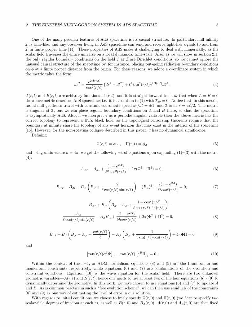
Figure 9: φ,Z(Z, T ) (see (42) for the definition of Z and T coordinates), for gaussian initial (27) data withP = 0.133059219, σ = 0.05, n = 1 and r0 = 0.2 in an ℓ = 2/π cosmology. This function of φ is scale-invariant in the critical regime, which unfolds roughly between T ≈ 8 and T ≈ 19 (though, interestingly, thescale-invariance seems to persist for longer in the scalar field than the geometric quantities—see Figs. 11and 12).

Figure 10: φ,ZZ(Z, T ), i.e. the derivative of the function plotted in Fig. 9.

3 RESULTS 19

Figure 11: The mass aspect, M(Z, T ), for the same solution shown in Fig. 9. That M becomes slightlynon-monotonic at late times is probably due to numerical error—this is a super-critical evolution, and themetric variables are already growing rapidly around T = 19.

Figure 12: The Ricci scalar multiplied by r2 (a scale-invariant combination in the critical regime) for thesame solution shown in Fig. 9.

3 RESULTS 20

Figure 13: A composite of the scale-invariant function φ,ZZ(Z, T ) for the near critical solutions of the fourfamilies of initial data considered, demonstrating universality of the solution in the critical limit. The datais plotted at T = 13 (compare Fig. 10). The harmonic profile appears somewhat different than the othersdue to a slicing effect, as explained in the text (also see Figs. 14 and 15). See Fig. 16 for the values of P ⋆

for each family.

amplitudes one could tune to a threshold solution after several light-crossing times, and perhaps then onewould more cleanly uncover the critical solution.

To give more evidence that all the solutions are indeed approaching a universal one in the critical regime,we need to compare them on a common spacetime slice. In Fig. 15 we show the same function of the scalarfield as in Fig. 13 transformed to a Christodoulou type coordinate system (r, v), where a v = constant curveis an ingoing null geodesic [20]. We normalized v so that dv = dtc at the origin; i.e. v also measures centralproper time. Thus comparing solutions on the same v = constant surface removes any slicing ambiguity 6.As can be seen from the figure, the transformed solutions are all quite similar, though we lose some accuracyin the transformation (which is why we have elected not to use these coordinates in all of the plots in Figs.9 - 13).

3.2.1 The scaling exponent γ

Another characteristic feature of Type II critical behavior in gravitational collapse is the universal scalingexponent γ in the relation M = K(p− p⋆)2γ . To measure this relationship in the current context, one needsto wait for the system to settle down to a steady-state to ensure that the apparent horizon is coincidentwith the event horizon, and hence that the mass estimate (38) gives the correct mass. In AdS, the boundaryconditions at I prevent us from performing this measurement—initially outgoing radiation that did notcontribute to the near-critical black hole formation will eventually reflect off I and pollute our measurement.However, as discussed by Garfinkle and Duncan [12], in the near-critical regime (above or below p⋆) anyquantity with dimension Lq, where L is a length scale, should exhibit a scaling relation with an exponentof qγ. Thus, following those authors, we find the maximum value attained by the Ricci scalar R at r = 0in sub-critical evolution for tc < 0. Plots of maxt<tc

ln |R(0, t)| vs. ln(P ⋆ − P ) for the four families studied

6we are grateful to David Garfinkle for suggesting this procedure to us

3 RESULTS 21

Figure 14: The Lorentz gamma factor W (43) between r = constant observer world-lines and those travellingnormal to the hypersurface tc = constant, at T = 13 for the 4 near-critical solutions as in Fig. 13. Thedifference between the three initially ingoing families and the harmonic one indicates that we are lookingat differing slices of spacetime as we move away from r = 0. In fact, the discontinuous peak in γ for theharmonic solution at around Z = −10.2 shows that the r = constant surface has become space-like to theright of this point, indicating a region undergoing gravitational collapse.

3 RESULTS 22

Figure 15: The function φ,ZZ(Z, v) for the same solutions shown in Fig. 13. v = constant is an ingoingnull geodesic, chosen here to intersect the origin at T = − ln tc = 13 in all cases, and along this hypersurfacewe plot as a function of Z = ln r. This coordinate system completely fixes the spacetime slice along whichwe are comparing solutions (at the expense of some loss of accuracy during the transformation), and givesadditional evidence that there is a universal critical solution.

3 RESULTS 23

is shown in Fig. 16. Since R ∝ L−2, these figures show that the scaling exponent γ of the 2+1D AdSKlein-Gordon system is about 1.2 ± 0.05.

Notice that the mass aspect M as defined in (33) is dimensionless (which is consistent with the scale-invariance of M as plotted in Fig. 11). On the other hand, when we keep ℓ fixed and vary P , the resultingblack hole mass (being proportional to r2

ah) has a length scale of 2, so one would expect the mass-parameterscaling relationship for BTZ black holes to go like M = K(P −P ⋆)2γ , where γ is the same value 1.15− 1.25found above for the scaling of R. The initial-mass estimate curves as shown in Figs. 4 and 5 do roughlyexhibit this scaling behavior for P > P ⋆.

3.2.2 Critical behavior in the presence of a point particle

Here we briefly show how the presence of a point particle (angle deficit) alters the critical solution. Theparticle contributes to the mass of the spacetime (36), so the more massive the particle (up to the maximumMPP = 1 in our units) the less scalar field energy is needed to form a black hole, and consequently we havesmaller amplitudes, P ⋆, at threshold. Interestingly, we find the same critical solution in all cases (see Fig.17 for 3 examples), the only noticeable differences being a systematic phase shift in T related to the mass ofthe particle. The kink-like transition in the mass aspect has the same shape as well, but it ranges from theparticle mass at r = 0 to M = 0. To within the resolution of our simulations (which was at 2048 grid-pointsin this case) the critical exponent is also the same, namely within the range γ = 1.15 to 1.25.

3.2.3 The critical solution from a CSS ansatz?

Given that we have self-similar behavior in the critical regime, it would be useful to find the exact solutionassuming a CSS ansatz. Traditionally this is done by assuming the existence of a homothetic Killing vector.ξ (see [6])

Lξgab = 2gab. (44)

This implies that in coordinates adapted to the homotheticity, so that ξ = ∂/∂τ , each component of gab hasthe form e2τf , for some function f independent of τ . Furthermore, LξRab = 0, so that Rab and hence theEinstein tensor Gab are independent of τ . This ansatz is not consistent with the field equations (1) in thepresence of the cosmological constant if we assume that the scalar field is self-similar (see [25]), as we observein the collapse simulations. Essentially, the scalar field stress-energy tensor (2) would need to decouple intoa piece that exactly cancels the cosmological constant term plus a scale-invariant term, but we do not thinkthat this is possible for a minimally-coupled scalar field.

It may be that in the 2+1D AdS system a different symmetry, such as a conformal Killing vector, wouldbe needed to generate the critical solution. Or perhaps the critical solution is only approximately homotheticover a limited region of the spacetime. Nevertheless, we have not yet found a symmetry-reduced system thatreproduces the observed critical behavior.7

3.3 Singularity structure

In all of the solutions that we have studied so far we find that after an apparent horizon forms what appearsto be a spacelike curvature singularity develops within the horizon. Specifically, the surface of excisionalong which the metric variables A and B and, consequently, the curvature invariants begin to diverge,is spacelike. By itself, demonstrating a spacelike surface of arbitrarily large curvature is not sufficient toprove that the singularity is spacelike—a counter-example would be the mass-inflation null singularity [22]8. However, if we extrapolate to the surface of infinite curvature, based upon the growth of the Ricci scalarprior to excision, we still find a spacelike surface (in fact, R grows so rapidly prior to excision —roughly like1/t4 along an r = constant surface if we translate t to zero at the singularity—that the surface of infinitecurvature essentially coincides with the excision surface at the resolution of Fig 19 below). In addition,

7Note added in preparation: David Garfinkle has very recently found a CSS solution in the limit where the cosmologicalconstant vanishes that appears to quite accurately describe the critical solution that we have found [21]. His result is quiteintriguing—the cosmological constant is essential for black holes to form, yet apparently it plays very little role in the solutionat the threshold of formation!

8We are grateful to Lior Burko for pointing this out to us

3 RESULTS 24

Figure 16: The maximum of ln |R(0, t < tc)| as a function of ln(P ⋆−P ) for sub-critical (P < P ⋆) evolutionsof the 4 families of initial data considered. These plots indicate that the maximum of R(0, t < tc) attainedduring evolution is proportional to (P ⋆ − P )−2γ , with γ ≈ 1.15 − 1.25.

3 RESULTS 25

Figure 17: A composite of the scale-invariant function φ,ZZ(Z, T ) at T = 13 for the near critical solutions ofthe gaussian family (σ = 0.05, r0 = 0.2) with 4 different initial values for A(0, 0)—0, 1, 2 and 3, correspondingto the presence of point particles at the origin with masses 0, 0.864665, 0.981684 and 0.997521 respectively(36). It is striking that these solutions only differ by a phase in T related to the particle masses; theyhave evolved to the same amplitude after starting with quite different initial amplitudes (namely, P ≈0.13, 0.078, 0.034, 0.013 from A = 0 to 3).

4 CONCLUDING REMARKS 26

B(t, r) → −∞ along this surface, indicating that the proper circumference measure ℓ tan(r/ℓ)eB goes tozero there (see Fig. 20 below). Thus, as with vacuum BTZ black holes, this singularity is crushing9: anyextended object reaching the singularity is forced to zero proper circumference, regardless of any angularmomentum or internal pressures that the object might have.

Figs. 18 and 19 are spacetime plots (essentially Penrose diagrams) of Φ(r, t) and the Ricci scalar R(r, t),respectively, for a gaussian initial pulse with P = 0.133051. On the pictures we have superimposed the regionof trapped surfaces and the inferred event horizon of the space time, found by tracing a null ray backwardsin time from the place where the AH meets I on the coordinate grid. Fig. 20 show contours of propercircumference for the same solution. The point P = 0.133051 in parameter space is slightly sub-critical (aswe have defined criticality, see Sec. 3.2)—a black hole forms because the bit of outgoing energy present att = 0 bounces off I and falls back onto the nearly collapsed scalar field, pushing it over the limit. This givesus a very clear view of the interior structure; for a more massive pulse the singularity forms shortly after theinitial implosion, resulting in a thin sliver of an interior in (r, t) coordinates.

From Fig. 19 one can see a striking peak that forms in R after the scalar field has bounced through theorigin and is travelling outwards. In this particular case R has a value of order −1010 in the interior, it thengrows to order +108 over a very short distance before decreasing to the AdS value of −6/ℓ2 ≈ −15. Thisnear-discontinuous behavior in R is characteristic of sub-critical evolutions, and becomes more extreme asone nears the critical solution.

As one approaches the excised space-like surface in Fig. 19, R starts to grow very rapidly, reaching valuesup to |1028| before excision (this may not be clear on the figure—we chose the gray scale to highlight thenear-discontinuous behavior in R). R actually oscillates between large positive and negative values alongthis surface, but our calculations are not sufficiently accurate to conclude that the oscillation is genuine. Inparticular, R is extremely sensitive to the difference Π2 − Φ2 (see (11)), and Π2 is usually around the sameorder of magnitude as Φ2 there. We also note that the maximum value attained by R along the excisedsurface becomes smaller towards I. This is to be expected, since in the 2+1D system, some scalar field isnecessary to produce a value of R differing from the AdS value (again, see (11)), and as we move towards Ialong the excised surface there is progressively less scalar field energy remaining.

4 Concluding remarks

We have studied black hole formation from the collapse of a minimally-coupled massless scalar field in 2+1dimensional AdS spacetime. Outside of the event horizon the spacetime settles down to a BTZ form; inthe interior a central, spacelike curvature singularity develops. At the threshold of black hole formation wefind that the scalar field and spacetime geometry evolve towards a universal, continuously self-similar form.When a point particle is present at the origin the critical solution is shifted in central proper time by anamount related to the mass of the particle.

By examining the behavior of the curvature scalar during sub-critical evolution we deduced that theuniversal scaling exponent γ for this system is roughly 1.2 ± 0.05. This value is quite different from thescaling exponent 1/2 derived by Peleg and Steif [9] for the collapse of thin rings of dust and by Birminghamand Sen [10] for particle collisions. However, those works considered different forms of matter, and the phasetransition was between black hole and naked singularity formation. Thus one would not expect the sameexponent. Also, the local spacetime geometry about a dust ring or point-particles is necessarily (empty)AdS, hence such systems cannot exhibit any of the features, other than mass scaling, that are characteristicof critical gravitational collapse.

Some questions remain unanswered in this work. First, what is the exact nature of the critical solution?In other words, what is the character of the symmetry (if any) responsible for the self-similar behaviour, asthe system does not appear to admit a global homothetic Killing vector 10. Second, will any distribution

9or deformationally strong, see [23]. It is straight-forward (though tedious) to see that r = 0 in the non-rotating BTZ blackhole is a strong singularity as defined by Tipler (though it is not a curvature singularity!). We have not repeated the formalcalculations in terms of Jacobi fields in our collapse simulations, but because of the central, space-like nature of the singularityback-reaction is not likely to weakening it. Note added in revision: shortly after this paper was first published, Lior Burkostudied the structure of the singularity in 2+1D AdS spacetime using a ‘qausi-homogenious’ approximation, and did find thesingularity to be strong and spacelike [24].

10though, as mentioned in the footnote of sec. 3.2.3, David Garfinkle has found a CSS solution that is apparently relevant to

4 CONCLUDING REMARKS 27

rscale (log)

0.0

1.2 x 10 4Φ

t

1.25

0

even

t hor

izon

region of trapped surfaces

excised region

−2.2 x 10 3

1

Figure 18: The gradient of the scalar field Φ(r, t) on the entire solution domain for a gaussian withP = 0.133051. On this picture we have also outlined the region of spacetime containing trapped surfaces,and drawn in the event horizon with a dashed line (found by tracing a null ray backwards in time fromthe place where the AH reaches r = 1—which is also I, so our coordinate system breaks down there). Westop the simulation at points where the metric variables begin to diverge (the lower boundary of the excisedregion), which presumably is just before a spacetime singularity forms (see Fig 19 for a similar plot of thecurvature scalar).

4 CONCLUDING REMARKS 28

rscale (log)

0.0

1.6 x 10 25Ricci scalar

t

1.25

0

even

t hor

izon

region of trapped surfaces

excised region

−1.1 x 10 28

1

1.0 x 10 13

−1.0 x 10 13

Figure 19: A plot of the Ricci scalar R(r, t) for the same solution as shown in Fig. 18. During most ofthe evolution |R| is bounded above by ≈ 1013, but shortly before reaching the excision boundary R startsto diverge rapidly, signaling the formation of a spacelike singularity.

4 CONCLUDING REMARKS 29

r

10−7

Contours of constant proper circumference

t

1.25

0

surface of excision

1

10−6

3x10−6

10−5

2x10−3

0.03

0.15

0.37

0.76

1.72

4.0 14

infinity

Figure 20: A contour plot of proper circumference (divided by 2π) r = ℓ tan(r/ℓ)eB for the same solutionas shown in Fig. 18 (the thickness of each contour line is constant in units of proper circumference). Thisplot demonstrates the central nature of the singularity. Along the excised surface approaching I r alsotends towards zero, though it is not clear with the limited resolution of this figure there. The event horizonasymptotes to r = 0.037, i.e. just outside the r = 0.03 contour.

REFERENCES 30

of energy that could conceivably form a black hole (i.e. with asymptotic mass M > 0) eventually do so ifone waits long enough (because of the Dirichlet boundary conditions imposed on the scalar field at I)? Athird question, related to the first two, is whether the critical solution we have found is a true black-hole-formation threshold solution. In other words, that we have a found a universal, CSS solution via a fine-tuningprocess indicates that this critical solution is one-mode unstable; so, does perturbing the critical solution“one way” result in a black hole, and perturbing it the “other way” cause the scalar field to remain regular,never forming a black hole? The asymptotic nature of AdS spacetime, which is ultimately responsible forthe boundary conditions of the scalar field at I, prevent us from answering this question in our collapsesimulations.

With regards to future work, it would be useful to extend these results to different scalar-field/geometrycouplings, include a mass and potential terms in the Lagrangian, and to add angular momentum to theinitial data to study the formation of rotating black holes. It would also be interesting to understand thecritical behavior in light of the AdS/CFT correspondence. Even though our calculation is purely classical,there should be a regime where the classical evolution is a good approximation to the full bulk theory, andconsequently there should be a dual CFT description of the critical phenomena.

Acknowledgements We would like to thank David Garfinkle, Viqar Husain, Lior Burko, Inaki Olabarrieta,Michel Olivier, Bill Unruh, Jason Ventrella, and Don Witt for many stimulating discussions. We are gratefulto David Garfinkle for suggesting to us the method we used to obtain γ, as well as the use of the ingoing nullcoordinate system to compare near-critical solutions. MWC would particularly like to thank Robert Mannfor many early discussions about this problem during the 1999 Classical and Quantum Physics of Strong

Gravitational Fields program held at the Institute for Theoretical Physics, UC Santa Barbara. This workwas supported by NSERC and by NSF PHY97-22068 and PHY94-07194. Most calculations were carried outon the vn.physics.ubc.ca Beofwulf cluster which was funded by the Canadian Foundation for Innovation.

References

[1] M. Banados, C. Teitelboim and J. Zanelli, Phys. Rev. Lett. 69, 1849 (1992)

[2] J. M. Maldacena, Adv. Theor. Math. Phys. 2, 231 (1998), hep-th/9711200.

[3] M. Banados, M. Henneaux, C. Teitelboim and J. Zanelli, Phys. Rev. D. 48, 1506 (1993),for generalizations to higher dimensions and multi-black holes seeD. Brill, Phys. Rev. D53, R4133 (1996),A. Steif, Phys. Rev. D53, 5527 (1996),S. Aminneborg, I. Bengtsson, S. Holst and P. Peldan, Class. Quant. Grav. 13, 2707 (1996), gr-qc/9604005

[4] S. Carlip, Class. Quant. Grav. 12, 2853 (1995),R.B. Mann, “Topological Black Holes—Outside Looking In”, gr-qc/9709039.

[5] M. Choptuik, Phys. Rev. Lett. 70, 9 (1993).

[6] C. Gundlach, “Critical phenomena in gravitational collapse”, Living Reviews 1999-4

[7] R. Mann and S. Ross, Phys. Rev. D47, 3319 (1993),W.L. Smith and R.B. Mann, Phys.Rev. D56, 4942 (1997)

[8] V. Husain, Phys. Rev. D50, 2361 (1994)K. S. Virbhadra Pramana 44, 317 (1995)

[9] Y. Peleg and A. R. Steif, Phys. Rev. D51, 3992 (1995), gr-qc/9412023.U. Danielsson, E. Keski-Vakkuri and M. Kruczenski, JHEP 0002, 039 (2000), hep-th/9912209U. Danielsson, E. Keski-Vakkuri and M. Kruczenski, Nucl. Phys. B563, 279 (1999)

the AdS critical solution [21]

REFERENCES 31

[10] H. Matschull, Class. Quant. Grav. 16, 1069 (1999),D. Birmingham and S. Sen, Phys.Rev.Lett. 84, 1074 (2000), hep-th/9908150

[11] V. Husain and M. Olivier, “Scalar field collapse in three-dimensional AdS spacetime”, gr-qc/0008060(2000).

[12] D. Garfinkle and G.C. Duncan, Phys.Rev. D58, 064024 (1998)

[13] R.M. Wald General Relativity, Chicago IL, University of Chicago Press 1984

[14] S.W. Hawking and G.F.R. Ellis, The Large Scale Structure of Space-Time (Cambridge: CambridgeUniversity Press)

[15] G.J. Galloway, K. Schleich, D.M. Witt and E. Woolgar, Phys. Rev. D60,104039 (1999)

[16] H. Kreiss and J. Oliger, “Methods for the Approximate Solution of Time Dependent Problems”, Global

Atmospheric Research Programme, Publications Series No. 10. (1973)

[17] R.L. Marsa and M.W. Choptuik, “The RNPL User’s Guide”,http://laplace.physics.ubc.ca/Members/marsa/rnpl/users guide/users guide.html (1995)

[18] http://laplace.physics.ubc.ca/People/fransp/index.html

[19] W.G. Unruh (1984), private communication

[20] see D. Christodoulou, Class. Quant. Grav. 16, A23 (1999), and references therein

[21] D. Garfinkle, “An exact solution for 2+1 dimensional critical collapse”, gr-qc/0008023 (2000)

[22] E. Poisson and W. Israel, Phys. Rev. D 41, 1796 (1990)

[23] F.J. Tipler, Phys. Lett. A 64A, 8 (1977),A. Ori Phys. Rev. D61, 064016 (2000),B.C. Nolan, Phys.Rev. D62, 044015 (2000), gr-qc/0001026

[24] L.M. Burko, “Singularity in 2+1 dimensional AdS-scalar black hole”, gr-qc/0008043 (2000).

[25] P.R. Brady, Phys.Rev. D51,4168 (1995).