Graphs, Principal Minors, and Eigenvalue Problemsby

John C. Urschel

Submitted to the Department of Mathematicsin partial fulfillment of the requirements for the degree of

Doctor of Philosophy in Mathematics

at the

MASSACHUSETTS INSTITUTE OF TECHNOLOGY

September 2021

© John C. Urschel, MMXXI. All rights reserved.

The author hereby grants to MIT permission to reproduce and to distributepublicly paper and electronic copies of this thesis document in whole or in

part in any medium now known or hereafter created.

Author . . . . . . . . . . . . . . . . . . . . . . . . . . . . . . . . . . . . . . . . . . . . . . . . . . . . . . . . . . . . . .Department of Mathematics

August 6, 2021

Certified by . . . . . . . . . . . . . . . . . . . . . . . . . . . . . . . . . . . . . . . . . . . . . . . . . . . . . . . . .Michel X. Goemans

RSA Professor of Mathematics and Department HeadThesis Supervisor

Accepted by . . . . . . . . . . . . . . . . . . . . . . . . . . . . . . . . . . . . . . . . . . . . . . . . . . . . . . . . .Jonathan Kelner

Chairman, Department Committee on Graduate Theses

2

Graphs, Principal Minors, and Eigenvalue Problems

by

John C. Urschel

Submitted to the Department of Mathematicson August 6, 2021, in partial fulfillment of the

requirements for the degree ofDoctor of Philosophy in Mathematics

AbstractThis thesis considers four independent topics within linear algebra: determinantal pointprocesses, extremal problems in spectral graph theory, force-directed layouts, and eigenvaluealgorithms. For determinantal point processes (DPPs), we consider the classes of symmetricand signed DPPs, respectively, and in both cases connect the problem of learning theparameters of a DPP to a related matrix recovery problem. Next, we consider two conjecturesin spectral graph theory regarding the spread of a graph, and resolve both. For force-directedlayouts of graphs, we connect the layout of the boundary of a Tutte spring embedding totrace theorems from the theory of elliptic PDEs, and we provide a rigorous theoreticalanalysis of the popular Kamada-Kawai objective, proving hardness of approximation andstructural results regarding optimal layouts, and providing a polynomial time randomizedapproximation scheme for low diameter graphs. Finally, we consider the Lanczos methodfor computing extremal eigenvalues of a symmetric matrix and produce new error estimatesfor this algorithm.

Thesis Supervisor: Michel X. GoemansTitle: RSA Professor of Mathematics and Department Head

3

4

Acknowledgments

I would like to thank my advisor, Michel Goemans. From the moment I met him, I was

impressed and inspired by the way he thinks about mathematics. Despite his busy schedule

as head of the math department, he always made time when I needed him. He has been the

most supportive advisor a student could possibly ask for. He’s the type of mathematician

I aspire to be. I would also like to thank the other members of my thesis committee,

Alan Edelman and Philippe Rigollet. They have been generous with their time and their

mathematical knowledge. In my later years as a PhD candidate, Alan has served as a

secondary advisor of sorts, and I’m thankful for our weekly Saturday meetings.

I’ve also been lucky to work with a number of great collaborators during my time at

MIT. This thesis would not have been possible without my mathematical collaborations and

conversations with Jane Breen, Victor-Emmanuel Brunel, Erik Demaine, Adam Hesterberg,

Fred Koehler, Jayson Lynch, Ankur Moitra, Alex Riasanovksy, Michael Tait, and Ludmil

Zikatanov. And, though the associated work does not appear in this thesis, I am also grateful

for collaborations with Xiaozhe Hu, Dhruv Rohatgi, and Jake Wellens during my PhD.

I’ve been the beneficiary of a good deal of advice, mentorship, and support from the larger

mathematics community. This group is too long to list, but I’m especially grateful to Rediet

Abebe, Michael Brenner, David Mordecai, Jelani Nelson, Peter Sarnak, Steven Strogatz,

and Alex Townsend, among many others, for always being willing to give me some much

needed advice during my time at MIT.

I would like to thank my office mates, Fred Koehler and Jake Wellens (and Megan Fu),

for making my time in office 2-342 so enjoyable. With Jake’s wall mural and very large

and dusty rug, our office felt lived in and was a comfortable place to do math. I’ve had

countless interesting conversations with fellow grad students, including Michael Cohen,

Younhun Kim, Meehtab Sawhney, and Jonathan Tidor, to name a few. My interactions with

MIT undergrads constantly reminded me just how fulfilling and rewarding mentorship can

be. I’m thankful to all the support staff members at MIT math, and have particularly fond

memories of grabbing drinks with André at the Muddy, constantly bothering Michele with

5

whatever random MIT problem I could not solve, and making frequent visits to Rosalee for

more espresso pods. More generally, I have to thank the entire math department for fostering

such a warm and welcoming environment to do math. MIT math really does feel like home.

I’d be remiss if I did not thank my friends and family for their non-academic contributions.

I have to thank Ty Howle for supporting me every step of the way, and trying to claim

responsibility for nearly all of my mathematical work. This is a hard claim to refute, as it

was often only once I took a step back and looked at things from a different perspective that

breakthroughs were made. I’d like to thank Robert Hess for constantly encouraging and

believing in me, despite knowing absolutely no math. I’d like to thank my father and mother

for instilling a love of math in me from a young age. My fondest childhood memories of

math were of going through puzzle books at the kitchen table with my mother, and leafing

through the math section in the local Chapters in St. Catherines while my father worked

in the cafe. I’d like to thank Louisa for putting up with me, moving with me (eight times

during this PhD), and proofreading nearly all of my academic papers. I would thank Joanna,

but, frankly, she was of little to no help.

This research was supported in part by ONR Research Contract N00014-17-1-2177.

During my time at MIT, I was previously supported by a Dean of Science Fellowship and

am currently supported by a Mathworks Fellowship, both of which have allowed me to place

a greater emphasis on research, and without which this thesis, in its current form, would not

have been possible.

6

For John and Venita

7

8

Contents

1 Introduction 11

2 Determinantal Point Processes and Principal Minor Assignment Problems 17

2.1 Introduction . . . . . . . . . . . . . . . . . . . . . . . . . . . . . . . . . . 17

2.1.1 Symmetric Matrices . . . . . . . . . . . . . . . . . . . . . . . . . 18

2.1.2 Magnitude-Symmetric Matrices . . . . . . . . . . . . . . . . . . . 20

2.2 Learning Symmetric Determinantal Point Processes . . . . . . . . . . . . . 22

2.2.1 An Associated Principal Minor Assignment Problem . . . . . . . . 22

2.2.2 Definition of the Estimator . . . . . . . . . . . . . . . . . . . . . . 25

2.2.3 Information Theoretic Lower Bounds . . . . . . . . . . . . . . . . 29

2.2.4 Algorithmic Aspects and Experiments . . . . . . . . . . . . . . . . 32

2.3 Recovering a Magnitude-Symmetric Matrix from its Principal Minors . . . 38

2.3.1 Principal Minors and Magnitude-Symmetric Matrices . . . . . . . . 40

2.3.2 Efficiently Recovering a Matrix from its Principal Minors . . . . . 60

2.3.3 An Algorithm for Principal Minors with Noise . . . . . . . . . . . 66

3 The Spread and Bipartite Spread Conjecture 75

3.1 Introduction . . . . . . . . . . . . . . . . . . . . . . . . . . . . . . . . . . 75

3.2 The Bipartite Spread Conjecture . . . . . . . . . . . . . . . . . . . . . . . 78

3.3 A Sketch for the Spread Conjecture . . . . . . . . . . . . . . . . . . . . . 85

3.3.1 Properties of Spread-Extremal Graphs . . . . . . . . . . . . . . . . 88

9

4 Force-Directed Layouts 95

4.1 Introduction . . . . . . . . . . . . . . . . . . . . . . . . . . . . . . . . . . 95

4.2 Tutte’s Spring Embedding and a Trace Theorem . . . . . . . . . . . . . . . 98

4.2.1 Spring Embeddings and a Schur Complement . . . . . . . . . . . . 101

4.2.2 A Discrete Trace Theorem and Spectral Equivalence . . . . . . . . 109

4.3 The Kamada-Kawai Objective and Optimal Layouts . . . . . . . . . . . . . 127

4.3.1 Structural Results for Optimal Embeddings . . . . . . . . . . . . . 131

4.3.2 Algorithmic Lower Bounds . . . . . . . . . . . . . . . . . . . . . 138

4.3.3 An Approximation Algorithm . . . . . . . . . . . . . . . . . . . . 147

5 Error Estimates for the Lanczos Method 151

5.1 Introduction . . . . . . . . . . . . . . . . . . . . . . . . . . . . . . . . . . 151

5.1.1 Related Work . . . . . . . . . . . . . . . . . . . . . . . . . . . . . 155

5.1.2 Contributions and Remainder of Chapter . . . . . . . . . . . . . . 157

5.2 Preliminary Results . . . . . . . . . . . . . . . . . . . . . . . . . . . . . . 159

5.3 Asymptotic Lower Bounds and Improved Upper Bounds . . . . . . . . . . 161

5.4 Distribution Dependent Bounds . . . . . . . . . . . . . . . . . . . . . . . 175

5.5 Estimates for Arbitrary Eigenvalues and Condition Number . . . . . . . . . 181

5.6 Experimental Results . . . . . . . . . . . . . . . . . . . . . . . . . . . . . 187

10

Chapter 1

Introduction

In this thesis, we consider a number of different mathematical topics in linear algebra, with

a focus on determinantal point processes and eigenvalue problems. Below we provide a

brief non-technical summary of each topic in this thesis, as well as a short summary of other

interesting projects that I had the pleasure of working on during my PhD that do not appear

in this thesis.

Determinantal Point Processes and Principal Minor Assignment Problems

A determinantal point process is a probability distribution over the subsets of a finite

ground set where the distribution is characterized by the principal minors of some fixed

matrix. Given a finite set, say, [𝑁 ] = 1, . . . , 𝑁 where 𝑁 is a positive integer, a DPP

is a random subset 𝑌 ⊆ [𝑁 ] such that 𝑃 (𝐽 ⊆ 𝑌 ) = det(𝐾𝐽), for all fixed 𝐽 ⊆ [𝑁 ],

where 𝐾 ∈ R𝑁×𝑁 is a given matrix called the kernel of the DPP and 𝐾𝐽 = (𝐾𝑖,𝑗)𝑖,𝑗∈𝐽 is

the principal submatrix of 𝐾 associated with the set 𝐽 . In Chapter 2, we focus on DPPs

with kernels that have two different types of structure. First, we restrict ourselves to DPPs

with symmetric kernels, and produce an algorithm that learns the kernel of a DPP from

its samples. Then, we consider the slightly broader class of DPPs with kernels that have

corresponding off-diagonal entries equal in magnitude, i.e., 𝐾 satisfies |𝐾𝑖,𝑗| = |𝐾𝑗,𝑖| for all

𝑖, 𝑗 ∈ [𝑁 ], and produce an algorithm to recover such a matrix 𝐾 from (possibly perturbed

versions of) its principal minors. Sections 2.2 and 2.3 are written so that they may be read

11

independently of each other. This chapter is joint work with Victor-Emmanuel Brunel,

Michel Goemans, Ankur Moitra, and Philippe Rigollet, and based on [119, 15].

The Spread and Bipartite Spread Conjecture

Given a graph 𝐺 = ([𝑛], 𝐸), [𝑛] = 1, ..., 𝑛, the adjacency matrix 𝐴 ∈ R𝑛×𝑛 of 𝐺

is defined as the matrix with 𝐴𝑖,𝑗 = 1 if 𝑖, 𝑗 ∈ 𝐸 and 𝐴𝑖,𝑗 = 0 otherwise. 𝐴 is a real

symmetric matrix, and so has real eigenvalues 𝜆1 ≥ ... ≥ 𝜆𝑛. One interesting quantity is

the difference between extreme eigenvalues 𝜆1 − 𝜆𝑛, commonly referred to as the spread of

the graph 𝐺. In [48], the authors proposed two conjectures. First, the authors conjectured

that if a graph 𝐺 of size |𝐸| ≤ 𝑛2/4 maximizes the spread over all graphs of order 𝑛

and size |𝐸|, then the graph is bipartite. The authors also conjectured that if a graph 𝐺

maximizes the spread over all graphs of order 𝑛, then the graph is the join (i.e., with all

edges in between) 𝐾⌊2𝑛/3⌋ ∨ 𝑒𝑛⌈𝑛/3⌉ of a clique of order ⌊2𝑛/3⌋ and an independent set

of order ⌈𝑛/3⌉. We refer to these conjectures as the bipartite spread and spread conjectures,

respectively. In Chapter 3, we consider both of these conjectures. We provide an infinite

class of counterexamples to the bipartite spread conjecture, and prove an asymptotic version

of the bipartite spread conjecture that is as tight as possible. In addition, for the spread

conjecture, we make a number of observations regarding any spread-optimal graph, and use

these observations to sketch a proof of the spread conjecture for all 𝑛 sufficiently large. The

full proof of the spread conjecture for all 𝑛 sufficiently large is rather long and technical,

and can be found in [12]. This chapter is joint work with Jane Breen, Alex Riasanovsky,

and Michael Tait, and based on [12].

Force-Directed Layouts

A force-directed layout, broadly speaking, is a technique for drawing a graph in a low-

dimensional Euclidean space (usually dimension ≤ 3) by applying “forces” between the

set of vertices and/or edges. In a force-directed layout, vertices connected by an edge (or

at a small graph distance from each other) tend to be close to each other in the resulting

layout. Two well-known examples of a force-directed layout are Tutte’s spring embedding

12

and metric multidimensional scaling. In his 1963 work titled “How to Draw a Graph,”

Tutte found an elegant technique to produce planar embeddings of planar graphs that also

minimize the sum of squared edge lengths in some sense. In particular, for a three-connected

planar graph, he showed that if the outer face of the graph is fixed as the complement of

some convex region in the plane, and every other point is located at the mass center of its

neighbors, then the resulting embedding is planar. This result is now known as Tutte’s spring

embedding theorem, and is considered by many to be the first example of a force-directed

layout [117]. One of the major questions that this result does not treat is how to best embed

the outer face. In Chapter 4, we investigate this question, consider connections to a Schur

complement, and provide some theoretical results for this Schur complement using a discrete

energy-only trace theorem. In addition, we also consider the later proposed Kamada-Kawai

objective, which can provide a force-directed layout of an arbitrary graph. In particular, we

prove a number of structural results regarding layouts that minimize this objective, provide

algorithmic lower bounds for the optimization problem, and propose a polynomial time

approximation scheme for drawing low diameter graphs. Sections 4.2 and 4.3 are written

so that they may be read independently of each other. This chapter is joint work with Erik

Demaine, Adam Hesterberg, Fred Koehler, Jayson Lynch, and Ludmil Zikatanov, and is

based on [124, 31].

Error Estimates for the Lanczos Method

The Lanczos method is one of the most powerful and fundamental techniques for solving

an extremal symmetric eigenvalue problem. Convergence-based error estimates depend

heavily on the eigenvalue gap, but in practice, this gap is often relatively small, resulting

in significant overestimates of error. One way to avoid this issue is through the use of

uniform error estimates, namely, bounds that depend only on the dimension of the matrix

and the number of iterations. In Chapter 5, we prove upper uniform error estimates for

the Lanczos method, and provide a number of lower bounds through the use of orthogonal

polynomials. In addition, we prove more specific results for matrices that possess some level

of eigenvalue regularity or whose eigenvalues converge to some limiting empirical spectral

13

distribution. Through numerical experiments, we show that the theoretical estimates of this

chapter do apply to practical computations for reasonably sized matrices. This chapter has

no collaborators, and is based on [122].

Topics not in this Thesis

During my PhD, I have had the chance to work on a number of interesting topics that

do not appear in this thesis. Below I briefly describe some of these projects. In [52] (joint

with X. Hu and L. Zikatanov), we consider graph disaggregation, a technique to break

high degree nodes of a graph into multiple smaller degree nodes, and prove a number of

results regarding the spectral approximation of a graph by a disaggregated version of it.

In [17] (joint with V.E. Brunel, A. Moitra, and P. Rigollet), we analyze the curvature of

the expected log-likelihood around its maximum and characterize of when the maximum

likelihood estimator converges at a parametric rate. In [120], we study centroidal Voronoi

tessellations from a variational perspective and show that, for any density function, there

does not exist a unique two generator centroidal Voronoi tessellation for dimensions greater

than one. In [121], we prove a generalization of Courant’s theorem for discrete graphs,

namely, that for the 𝑘𝑡ℎ eigenvalue of a generalized Laplacian of a discrete graph, there

exists a set of corresponding eigenvectors such that each eigenvector can be decomposed

into at most k nodal domains, and that this set is of co-dimension zero with respect to the

entire eigenspace. In [123] (joint with J. Wellens), we show that, given a graph with local

crossing number either at most 𝑘 or at least 2𝑘, it is NP-complete to decide whether the local

crossing number is at most 𝑘 or at least 2𝑘. In [97] (joint with D. Rohatgi and J. Wellens),

we treat two conjectures – one regarding the maximum possible value of 𝑐𝑝(𝐺) + 𝑐𝑝()

(where 𝑐𝑝(𝐺) is the minimum number of cliques needed to cover the edges of 𝐺 exactly

once), due to de Caen, Erdos, Pullman and Wormald, and the other regarding 𝑏𝑝𝑘(𝐾𝑛)

(where 𝑏𝑝𝑘(𝐺) is the minimum number of bicliques needed to cover each edge of 𝐺 exactly

𝑘 times), due to de Caen, Gregory and Pritikin. We disprove the first, obtaining improved

lower and upper bounds on 𝑚𝑎𝑥𝐺 𝑐𝑝(𝐺) + 𝑐𝑝(), and we prove an asymptotic version

of the second, showing that 𝑏𝑝𝑘(𝐾𝑛) = (1 + 𝑜(1))𝑛. If any of the topics (very briefly)

14

described here interest you, I encourage you to take a look at the associated paper. This

thesis was constructed to center around a topic and to be of a manageable length, and I am

no less proud of some of the results described here that do not appear in this thesis.

15

16

Chapter 2

Determinantal Point Processes and

Principal Minor Assignment Problems

2.1 Introduction

A determinantal point process (DPP) is a probability distribution over the subsets of a finite

ground set where the distribution is characterized by the principal minors of some fixed

matrix. DPPs emerge naturally in many probabilistic setups such as random matrices and

integrable systems [10]. They also have attracted interest in machine learning in the past

years for their ability to model random choices while being tractable and mathematically

elegant [71]. Given a finite set, say, [𝑁 ] = 1, . . . , 𝑁 where 𝑁 is a positive integer, a

DPP is a random subset 𝑌 ⊆ [𝑁 ] such that 𝑃 (𝐽 ⊆ 𝑌 ) = det(𝐾𝐽), for all fixed 𝐽 ⊆ [𝑁 ],

where 𝐾 ∈ R𝑁×𝑁 is a given matrix called the kernel of the DPP and 𝐾𝐽 = (𝐾𝑖,𝑗)𝑖,𝑗∈𝐽

is the principal submatrix of 𝐾 associated with the set 𝐽 . Assumptions on 𝐾 that yield

the existence of a DPP can be found in [14] and it is easily seen that uniqueness of the

DPP is then automatically guaranteed. For instance, if 𝐼 − 𝐾 is invertible (𝐼 being the

identity matrix), then 𝐾 is the kernel of a DPP if and only if 𝐾(𝐼 −𝐾)−1 is a 𝑃0-matrix,

i.e., all its principal minors are nonnegative. We refer to [54] for further definitions and

properties of 𝑃0 matrices. Note that in that case, the DPP is also an 𝐿-ensemble, with

probability mass function given by 𝑃 (𝑌 = 𝐽) = det(𝐿𝐽)/ det(𝐼 + 𝐿), for all 𝐽 ⊆ [𝑁 ],

17

where 𝐿 = 𝐾(𝐼 −𝐾)−1.

DPPs with a symmetric kernel have attracted a lot of interest in machine learning because

they satisfy a property called negative association, which models repulsive interactions

between items [8]. Following the seminal work of Kulesza and Taskar [72], discrete

symmetric DPPs have found numerous applications in machine learning, including in

document and timeline summarization [76, 132], image search [70, 1] and segmentation

[73], audio signal processing [131], bioinformatics [6] and neuroscience [106]. What makes

such models appealing is that they exhibit repulsive behavior and lend themselves naturally

to tasks where returning a diverse set of objects is important. For instance, when applied to

recommender systems, DPPs enforce diversity in the items within one basket [45].

From a statistical point of view, DPPs raise two essential questions. First, what are the

families of kernels that give rise to one and the same DPP? Second, given observations

of independent copies of a DPP, how to recover its kernel (which, as foreseen by the first

question, is not necessarily unique)? These two questions are directly related to the principal

minor assignment problem (PMA). Given a class of matrices, (1) describe the set of all

matrices in this class that have a prescribed list of principal minors (this set may be empty),

(2) find one such matrix. While the first task is theoretical in nature, the second one is

algorithmic and should be solved using as few queries of the prescribed principal minors as

possible. In this work, we focus on the question of recovering a kernel from observations,

which is closely related to the problem of recovering a matrix with given principal minors.

In this chapter, we focus on symmetric DPPs (which, when clear from context, we simply

refer to as DPPs) and signed DPPs, a slightly larger class of kernels that only require

corresponding off-diagonal entries be symmetric in magnitude.

2.1.1 Symmetric Matrices

In the symmetric case, there are fast algorithms for sampling (or approximately sampling)

from a DPP [32, 94, 74, 75]. Marginalizing the distribution on a subset 𝐼 ⊆ [𝑁 ] and

conditioning on the event that 𝐽 ⊆ 𝑌 both result in new DPPs and closed form expressions

for their kernels are known [11]. All of this work pertains to how to use a DPP once we

18

have learned its parameters. However, there has been much less work on the problem of

learning the parameters of a symmetric DPP. A variety of heuristics have been proposed,

including Expectation-Maximization [46], MCMC [1], and fixed point algorithms [80]. All

of these attempt to solve a non-convex optimization problem, and no guarantees on their

statistical performance are known. Recently, Brunel et al. [16] studied the rate of estimation

achieved by the maximum likelihood estimator, but the question of efficient computation

remains open. Apart from positive results on sampling, marginalization and conditioning,

most provable results about DPPs are actually negative. It is conjectured that the maximum

likelihood estimator is NP-hard to compute [69]. Actually, approximating the mode of size

𝑘 of a DPP to within a 𝑐𝑘 factor is known to be NP-hard for some 𝑐 > 1 [22, 108]. The best

known algorithms currently obtain a 𝑒𝑘 + 𝑜(𝑘) approximation factor [88, 89].

In Section 2.2, we bypass the difficulties associated with maximum likelihood estimation

by using the method of moments to achieve optimal sample complexity. In the setting

of DPPs, the method of moments has a close connection to a principal minor assignment

problem, which asks, given some set of principal minors of a matrix, to recover the original

matrix, up to some equivalence class. We introduce a parameter ℓ, called the cycle sparsity

of the graph induced by the kernel 𝐾, which governs the number of moments that need to

be considered and, thus, the sample complexity. The cycle sparsity of a graph is the smallest

integer ℓ so that the cycles of length at most ℓ yield a basis for the cycle space of the graph.

We use a refined version of Horton’s algorithm [51, 2] to implement the method of moments

in polynomial time. Even though there are in general exponentially many cycles in a graph

to consider, Horton’s algorithm constructs a minimum weight cycle basis and, in doing so,

also reveals the parameter ℓ together with a collection of at most ℓ induced cycles spanning

the cycle space. We use such cycles in order to construct our method of moments estimator.

For any fixed ℓ ≥ 2 and kernel 𝐾 satisfying either |𝐾𝑖,𝑗| ≥ 𝛼 or 𝐾𝑖,𝑗 = 0 for all 𝑖, 𝑗 ∈ [𝑁 ],

our algorithm has sample complexity

𝑛 = 𝑂

((𝐶

𝛼

)2ℓ

+log𝑁

𝛼2𝜀2

)

19

for some constant 𝐶 > 1, runs in time polynomial in 𝑛 and 𝑁 , and learns the parameters

up to an additive 𝜀 with high probability. The (𝐶/𝛼)2ℓ term corresponds to the number of

samples needed to recover the signs of the entries in 𝐾. We complement this result with

a minimax lower bound (Theorem 2) to show that this sample complexity is in fact near

optimal. In particular, we show that there is an infinite family of graphs with cycle sparsity

ℓ (namely length ℓ cycles) on which any algorithm requires at least (𝐶 ′𝛼)−2ℓ samples to

recover the signs of the entries of 𝐾 for some constant 𝐶 ′ > 1. We also provide experimental

results that confirm many quantitative aspects of our theoretical predictions. Together, our

upper bounds, lower bounds, and experiments present a nuanced understanding of which

symmetric DPPs can be learned provably and efficiently.

2.1.2 Magnitude-Symmetric Matrices

Recently, DPPs with non-symmetric kernels have gained interest in the machine learning

community [14, 44, 3, 93]. However, for these classes, questions of recovery are significantly

harder in general. In [14], Brunel proposes DPPs with kernels that are symmetric in

magnitudes, i.e., |𝐾𝑖,𝑗| = |𝐾𝑗,𝑖|, for all 𝑖, 𝑗 = 1, . . . , 𝑁 . This class is referred to as signed

DPPs. A signed DPP is a generalization of DPPs which allows for both attractive and

repulsive behavior. Such matrices are relevant in machine learning applications, because

they increase the modeling power of DPPs. An essential assumption made in [14] is

that 𝐾 is dense, which simplifies the combinatorial analysis. We consider magnitude-

symmetric matrices, but without any density assumption. The problem becomes significantly

harder because it requires a fine analysis of the combinatorial properties of a graphical

representation of the sparsity of the matrix and the products of corresponding off-diagonal

entries. In Section 2.3, we treat both theoretical and algorithmic questions around recovering

a magnitude-symmetric matrix from its principal minors. First, in Subsection 2.3.1, we

show that, for a given magnitude-symmetric matrix 𝐾, the principal minors of length at

most ℓ, for some graph invariant ℓ depending only on principal minors of order one and

two, uniquely determine principal minors of all orders. Next, in Subsection 2.3.2, we

describe an efficient algorithm that, given the principal minors of a magnitude-symmetric

20

matrix, computes a matrix with those principal minors. This algorithm queries only 𝑂(𝑛2)

principal minors, all of a bounded order that depends solely on the sparsity of the matrix.

Finally, in Subsection 2.3.3, we consider the question of recovery when principal minors

are only known approximately, and construct an algorithm that, for magnitude-symmetric

matrices that are sufficiently generic in a sense, recovers the matrix almost exactly. This

algorithm immediately implies an procedure for learning a signed DPP from its samples, as

basic probabilistic techniques (e.g., a union bound, etc.) can be used to show that with high

probability all estimators are sufficiently close to the principal minor they are approximating.

21

2.2 Learning Symmetric Determinantal Point Processes

Let 𝑌1, . . . , 𝑌𝑛 be 𝑛 independent copies of 𝑌 ∼ DPP(𝐾), for some unknown kernel 𝐾 such

that 0 ⪯ 𝐾 ⪯ 𝐼𝑁 . It is well known that 𝐾 is identified by DPP(𝐾) only up to flips of the

signs of its rows and columns: If 𝐾 ′ is another symmetric matrix with 0 ⪯ 𝐾 ′ ⪯ 𝐼𝑁 , then

DPP(𝐾 ′)=DPP(𝐾) if and only if 𝐾 ′ = 𝐷𝐾𝐷 for some 𝐷 ∈ 𝒟𝑁 , where 𝒟𝑁 denotes the

class of all 𝑁 ×𝑁 diagonal matrices with only 1 and −1 on their diagonals [69, Theorem

4.1]. We call such a transform a 𝒟𝑁 -similarity of 𝐾.

In view of this equivalence class, we define the following pseudo-distance between

kernels 𝐾 and 𝐾 ′:

𝜌(𝐾,𝐾 ′) = inf𝐷∈𝒟𝑁

|𝐷𝐾𝐷 −𝐾 ′|∞ ,

where for any matrix 𝐾, |𝐾|∞ = max𝑖,𝑗∈[𝑁 ] |𝐾𝑖,𝑗| denotes the entrywise sup-norm.

For any 𝑆 ⊂ [𝑁 ], we write ∆𝑆 = det(𝐾𝑆), where 𝐾𝑆 denotes the |𝑆| × |𝑆| sub-matrix

of 𝐾 obtained by keeping rows and columns with indices in 𝑆. Note that for 1 ≤ 𝑖 = 𝑗 ≤ 𝑁 ,

we have the following relations:

𝐾𝑖,𝑖 = P[𝑖 ∈ 𝑌 ], ∆𝑖,𝑗 = P[𝑖, 𝑗 ⊆ 𝑌 ],

and |𝐾𝑖,𝑗| =√

𝐾𝑖,𝑖𝐾𝑗,𝑗 −∆𝑖,𝑗. Therefore, the principal minors of size one and two of

𝐾 determine 𝐾 up to the sign of its off-diagonal entries. What remains is to compute the

signs of the off-diagonal entries. In fact, for any 𝐾, there exists an ℓ depending only on the

graph 𝐺𝐾 induced by 𝐾, such that 𝐾 can be recovered up to a 𝒟𝑁 -similarity with only the

knowledge of its principal minors of size at most ℓ. We will show that this ℓ is exactly the

cycle sparsity.

2.2.1 An Associated Principal Minor Assignment Problem

In this subsection, we consider the following related principal minor assignment problem:

Given a symmetric matrix 𝐾 ∈ R𝑁×𝑁 , what is the minimal ℓ such that 𝐾 can be

recovered (up to 𝒟𝑁 -similarity), using principal minors ∆𝑆 , of size at most ℓ?

22

This problem has a clear relation to learning DPPs, as, in our setting, we can approximate

the principal minors of 𝐾 by empirical averages. However the accuracy of our estimator

deteriorates with the size of the principal minor, and we must therefore estimate the smallest

possible principal minors in order to achieve optimal sample complexity. Answering the

above question tells us how small of principal minors we can consider. The relationship

between the principal minors of 𝐾 and recovery of DPP(𝐾) has also been considered

elsewhere. There has been work regarding the symmetric principal minor assignment

problem, namely the problem of computing a matrix given an oracle that gives any principal

minor in constant time [96]. Here, we prove that the smallest ℓ such that all the principal

minors of 𝐾 are uniquely determined by those of size at most ℓ is exactly the cycle sparsity

of the graph induced by 𝐾.

We begin by recalling some standard graph theoretic notions. Let 𝐺 = ([𝑁 ], 𝐸),

|𝐸| = 𝑚. A cycle 𝐶 of 𝐺 is any connected subgraph in which each vertex has even degree.

Each cycle 𝐶 is associated with an incidence vector 𝑥 ∈ 𝐺𝐹 (2)𝑚 such that 𝑥𝑒 = 1 if 𝑒 is

an edge in 𝐶 and 𝑥𝑒 = 0 otherwise. The cycle space 𝒞 of 𝐺 is the subspace of 𝐺𝐹 (2)𝑚

spanned by the incidence vectors of the cycles in 𝐺. The dimension 𝜈𝐺 of the cycle space is

called the cyclomatic number, and it is well known that 𝜈𝐺 := 𝑚−𝑁 + 𝜅(𝐺), where 𝜅(𝐺)

denotes the number of connected components of 𝐺. Recall that a simple cycle is a graph

where every vertex has either degree two or zero and the set of vertices with degree two

form a connected set. A cycle basis is a basis of 𝒞 ⊂ 𝐺𝐹 (2)𝑚 such that every element is a

simple cycle. It is well known that every cycle space has a cycle basis of induced cycles.

Definition 1. The cycle sparsity of a graph 𝐺 is the minimal ℓ for which 𝐺 admits a cycle

basis of induced cycles of length at most ℓ, with the convention that ℓ = 2 whenever the

cycle space is empty. A corresponding cycle basis is called a shortest maximal cycle basis.

A shortest maximal cycle basis of the cycle space was also studied for other reasons by

[21]. We defer a discussion of computing such a basis to a later subsection. For any subset

𝑆 ⊆ [𝑁 ], denote by 𝐺𝐾(𝑆) = (𝑆,𝐸(𝑆)) the subgraph of 𝐺𝐾 induced by 𝑆. A matching

of 𝐺𝐾(𝑆) is a subset 𝑀 ⊆ 𝐸(𝑆) such that any two distinct edges in 𝑀 are not adjacent in

𝐺(𝑆). The set of vertices incident to some edge in 𝑀 is denoted by 𝑉 (𝑀). We denote by

23

ℳ(𝑆) the collection of all matchings of 𝐺𝐾(𝑆). Then, if 𝐺𝐾(𝑆) is an induced cycle, we

can write the principal minor ∆𝑆 = det(𝐾𝑆) as follows:

∆𝑆 =∑

𝑀∈ℳ(𝑆)

(−1)|𝑀 |∏

𝑖,𝑗∈𝑀

𝐾2𝑖,𝑗

∏𝑖 ∈𝑉 (𝑀)

𝐾𝑖,𝑖 + 2× (−1)|𝑆|+1∏

𝑖,𝑗∈𝐸(𝑆)

𝐾𝑖,𝑗. (2.1)

Proposition 1. Let 𝐾 ∈ R𝑁×𝑁 be a symmetric matrix, 𝐺𝐾 be the graph induced by 𝐾, and

ℓ ≥ 3 be some integer. The kernel 𝐾 is completely determined up to 𝒟𝑁 -similarity by its

principal minors of size at most ℓ if and only if the cycle sparsity of 𝐺𝐾 is at most ℓ.

Proof. Note first that all the principal minors of 𝐾 completely determine 𝐾 up to a 𝒟𝑁 -

similarity [96, Theorem 3.14]. Moreover, recall that principal minors of degree at most 2

determine the diagonal entries of 𝐾 as well as the magnitude of its off-diagonal entries.

In particular, given these principal minors, one only needs to recover the signs of the off-

diagonal entries of 𝐾. Let the sign of cycle 𝐶 in 𝐾 be the product of the signs of the entries

of 𝐾 corresponding to the edges of 𝐶.

Suppose 𝐺𝐾 has cycle sparsity ℓ and let (𝐶1, . . . , 𝐶𝜈) be a cycle basis of 𝐺𝐾 where each

𝐶𝑖, 𝑖 ∈ [𝜈] is an induced cycle of length at most ℓ. By (2.1), the sign of any 𝐶𝑖, 𝑖 ∈ [𝜈] is

completely determined by the principal minor ∆𝑆 , where 𝑆 is the set of vertices of 𝐶𝑖 and is

such that |𝑆| ≤ ℓ. Moreover, for 𝑖 ∈ [𝜈], let 𝑥𝑖 ∈ 𝐺𝐹 (2)𝑚 denote the incidence vector of 𝐶𝑖.

By definition, the incidence vector 𝑥 of any cycle 𝐶 is given by∑

𝑖∈ℐ 𝑥𝑖 for some subset

ℐ ⊂ [𝜈]. The sign of 𝐶 is then given by the product of the signs of 𝐶𝑖, 𝑖 ∈ ℐ and thus by

corresponding principal minors. In particular, the signs of all cycles are determined by the

principal minors ∆𝑆 with |𝑆| ≤ ℓ. In turn, by Theorem 3.12 in [96], the signs of all cycles

completely determine 𝐾, up to a 𝒟𝑁 -similarity.

Next, suppose the cycle sparsity of 𝐺𝐾 is at least ℓ + 1, and let 𝒞ℓ be the subspace of

𝐺𝐹 (2)𝑚 spanned by the induced cycles of length at most ℓ in 𝐺𝐾 . Let 𝑥1, . . . , 𝑥𝜈 be a basis

of 𝒞ℓ made of the incidence column vectors of induced cycles of length at most ℓ in 𝐺𝐾 and

form the matrix 𝐴 ∈ 𝐺𝐹 (2)𝑚×𝜈 by concatenating the 𝑥𝑖’s. Since 𝒞ℓ does not span the cycle

space of 𝐺𝐾 , 𝜈 < 𝜈𝐺𝐾≤ 𝑚. Hence, the rank of 𝐴 is less than 𝑚, so the null space of 𝐴⊤ is

non trivial. Let be the incidence column vector of an induced cycle 𝐶 that is not in 𝒞ℓ, and

24

let ℎ ∈ 𝐺𝐿(2)𝑚 with 𝐴⊤ℎ = 0, ℎ = 0 and ⊤ℎ = 1. These three conditions are compatible

because 𝐶 /∈ 𝒞ℓ. We are now in a position to define an alternate kernel 𝐾 ′ as follows: Let

𝐾 ′𝑖,𝑖 = 𝐾𝑖,𝑖 and |𝐾 ′

𝑖,𝑗| = |𝐾𝑖,𝑗| for all 𝑖, 𝑗 ∈ [𝑁 ]. We define the signs of the off-diagonal

entries of 𝐾 ′ as follows: For all edges 𝑒 = 𝑖, 𝑗, 𝑖 = 𝑗, sgn(𝐾 ′𝑒) = sgn(𝐾𝑒) if ℎ𝑒 = 0 and

sgn(𝐾 ′𝑒) = − sgn(𝐾𝑒) otherwise. We now check that 𝐾 and 𝐾 ′ have the same principal

minors of size at most ℓ but differ on a principal minor of size larger than ℓ. To that end, let

𝑥 be the incidence vector of a cycle 𝐶 in 𝒞ℓ so that 𝑥 = 𝐴𝑤 for some 𝑤 ∈ 𝐺𝐿(2)𝜈 . Thus

the sign of 𝐶 in 𝐾 is given by

∏𝑒 :𝑥𝑒=1

𝐾𝑒 = (−1)𝑥⊤ℎ

∏𝑒 :𝑥𝑒=1

𝐾 ′𝑒 = (−1)𝑤

⊤𝐴⊤ℎ∏

𝑒 :𝑥𝑒=1

𝐾 ′𝑒 =

∏𝑒 :𝑥𝑒=1

𝐾 ′𝑒

because 𝐴⊤ℎ = 0. Therefore, the sign of any 𝐶 ∈ 𝒞ℓ is the same in 𝐾 and 𝐾 ′. Now, let

𝑆 ⊆ [𝑁 ] with |𝑆| ≤ ℓ, and let 𝐺 = 𝐺𝐾𝑆= 𝐺𝐾′

𝑆be the graph corresponding to 𝐾𝑆 (or,

equivalently, to 𝐾 ′𝑆). For any induced cycle 𝐶 in 𝐺, 𝐶 is also an induced cycle in 𝐺𝐾 and

its length is at most ℓ. Hence, 𝐶 ∈ 𝒞ℓ and the sign of 𝐶 is the same in 𝐾 and 𝐾 ′. By [96,

Theorem 3.12], det(𝐾𝑆) = det(𝐾 ′𝑆). Next observe that the sign of 𝐶 in 𝐾 is given by

∏𝑒 : 𝑒=1

𝐾𝑒 = (−1)⊤ℎ

∏𝑒 : 𝑒=1

𝐾 ′𝑒 = −

∏𝑒 :𝑥𝑒=1

𝐾 ′𝑒.

Note also that since 𝐶 is an induced cycle of 𝐺𝐾 = 𝐺𝐾′ , the above quantity is nonzero. Let

𝑆 be the set of vertices in 𝐶. By (2.1) and the above display, we have det(𝐾𝑆) = det(𝐾 ′𝑆).

Together with [96, Theorem 3.14], it yields 𝐾 = 𝐷𝐾 ′𝐷 for all 𝐷 ∈ 𝒟𝑁 .

2.2.2 Definition of the Estimator

Our procedure is based on the previous result and can be summarized as follows. We first

estimate the diagonal entries (i.e., the principal minors of size one) of 𝐾 by the method of

moments. By the same method, we estimate the principal minors of size two of 𝐾, and we

deduce estimates of the magnitude of the off-diagonal entries. To use these estimates to

25

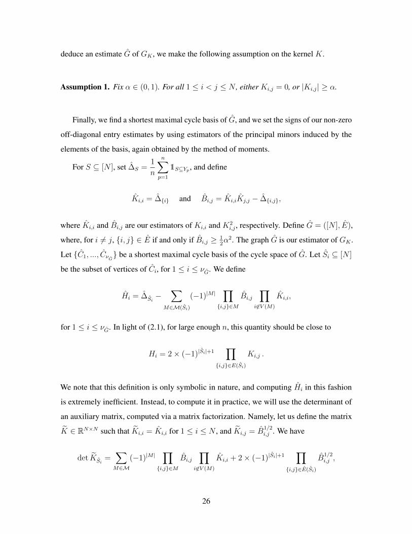
deduce an estimate of 𝐺𝐾 , we make the following assumption on the kernel 𝐾.

Assumption 1. Fix 𝛼 ∈ (0, 1). For all 1 ≤ 𝑖 < 𝑗 ≤ 𝑁 , either 𝐾𝑖,𝑗 = 0, or |𝐾𝑖,𝑗| ≥ 𝛼.

Finally, we find a shortest maximal cycle basis of , and we set the signs of our non-zero

off-diagonal entry estimates by using estimators of the principal minors induced by the

elements of the basis, again obtained by the method of moments.

For 𝑆 ⊆ [𝑁 ], set ∆𝑆 =1

𝑛

𝑛∑𝑝=1

1𝑆⊆𝑌𝑝 , and define

𝑖,𝑖 = ∆𝑖 and 𝑖,𝑗 = 𝑖,𝑖𝑗,𝑗 − ∆𝑖,𝑗,

where 𝑖,𝑖 and 𝑖,𝑗 are our estimators of 𝐾𝑖,𝑖 and 𝐾2𝑖,𝑗 , respectively. Define = ([𝑁 ], ),

where, for 𝑖 = 𝑗, 𝑖, 𝑗 ∈ if and only if 𝑖,𝑗 ≥ 12𝛼2. The graph is our estimator of 𝐺𝐾 .

Let 𝐶1, ..., 𝐶𝜈 be a shortest maximal cycle basis of the cycle space of . Let 𝑆𝑖 ⊆ [𝑁 ]

be the subset of vertices of 𝐶𝑖, for 1 ≤ 𝑖 ≤ 𝜈. We define

𝑖 = ∆𝑆𝑖−

∑𝑀∈ℳ(𝑆𝑖)

(−1)|𝑀 |∏

𝑖,𝑗∈𝑀

𝑖,𝑗

∏𝑖 ∈𝑉 (𝑀)

𝑖,𝑖,

for 1 ≤ 𝑖 ≤ 𝜈. In light of (2.1), for large enough 𝑛, this quantity should be close to

𝐻𝑖 = 2× (−1)|𝑆𝑖|+1∏

𝑖,𝑗∈𝐸(𝑆𝑖)

𝐾𝑖,𝑗 .

We note that this definition is only symbolic in nature, and computing 𝑖 in this fashion

is extremely inefficient. Instead, to compute it in practice, we will use the determinant of

an auxiliary matrix, computed via a matrix factorization. Namely, let us define the matrix𝐾 ∈ R𝑁×𝑁 such that 𝐾𝑖,𝑖 = 𝑖,𝑖 for 1 ≤ 𝑖 ≤ 𝑁 , and 𝐾𝑖,𝑗 = 1/2𝑖,𝑗 . We have

det 𝐾𝑆𝑖=∑𝑀∈ℳ

(−1)|𝑀 |∏

𝑖,𝑗∈𝑀

𝑖,𝑗

∏𝑖 ∈𝑉 (𝑀)

𝑖,𝑖 + 2× (−1)|𝑆𝑖|+1∏

𝑖,𝑗∈(𝑆𝑖)

1/2𝑖,𝑗 ,

26

so that we may equivalently write

𝑖 = ∆𝑆𝑖− det( 𝐾𝑆𝑖

) + 2× (−1)|𝑆𝑖|+1∏

𝑖,𝑗∈(𝑆𝑖)

1/2𝑖,𝑗 .

Finally, let = ||. Set the matrix 𝐴 ∈ 𝐺𝐹 (2)𝜈× with 𝑖-th row representing 𝐶𝑖 in

𝐺𝐹 (2)𝑚, 1 ≤ 𝑖 ≤ 𝜈, 𝑏 = (𝑏1, . . . , 𝑏𝜈) ∈ 𝐺𝐹 (2)𝜈 with 𝑏𝑖 = 12[sgn(𝑖) + 1], 1 ≤ 𝑖 ≤ 𝜈,

and let 𝑥 ∈ 𝐺𝐹 (2)𝑚 be a solution to the linear system 𝐴𝑥 = 𝑏 if a solution exists, 𝑥 = 1𝑚

otherwise. We define 𝑖,𝑗 = 0 if 𝑖, 𝑗 /∈ and 𝑖,𝑗 = 𝑗,𝑖 = (2𝑥𝑖,𝑗 − 1)1/2𝑖,𝑗 for all

𝑖, 𝑗 ∈ .

Next, we prove the following lemma which relates the quality of estimation of 𝐾 in

terms of 𝜌 to the quality of estimation of the principal minors ∆𝑆 .

Lemma 1. Let 𝐾 satisfy Assumption 1, and let ℓ be the cycle sparsity of 𝐺𝐾 . Let 𝜀 > 0. If

|∆𝑆 −∆𝑆| ≤ 𝜀 for all 𝑆 ⊆ [𝑁 ] with |𝑆| ≤ 2 and if |∆𝑆 −∆𝑆| ≤ (𝛼/4)|𝑆| for all 𝑆 ⊆ [𝑁 ]

with 3 ≤ |𝑆| ≤ ℓ, then

𝜌(,𝐾) < 4𝜀/𝛼 .

Proof. We can bound |𝑖,𝑗 −𝐾2𝑖,𝑗|, namely,

𝑖,𝑗 ≤ (𝐾𝑖,𝑖 + 𝛼2/16)(𝐾𝑗,𝑗 + 𝛼2/16)− (∆𝑖,𝑗 − 𝛼2/16)

≤ 𝐾2𝑖,𝑗 + 𝛼2/4

and

𝑖,𝑗 ≥ (𝐾𝑖,𝑖 − 𝛼2/16)(𝐾𝑗,𝑗 − 𝛼2/16)− (∆𝑖,𝑗 + 𝛼2/16)

≥ 𝐾2𝑖,𝑗 − 3𝛼2/16,

giving |𝑖,𝑗 −𝐾2𝑖,𝑗| < 𝛼2/4. Thus, we can correctly determine whether 𝐾𝑖,𝑗 = 0 or |𝐾𝑖,𝑗| ≥

𝛼, yielding = 𝐺𝐾 . In particular, the cycle basis 𝐶1, . . . , 𝐶𝜈of is a cycle basis of 𝐺𝐾 .

27

Let 1 ≤ 𝑖 ≤ 𝜈. Denote by 𝑡 = (𝛼/4)|𝑆𝑖|. We have

𝑖 −𝐻𝑖

≤ |∆𝑆𝑖

−∆𝑆𝑖|+ |ℳ(𝑆𝑖)|max

𝑥∈±1

[(1 + 4𝑡𝑥)|𝑆𝑖| − 1

]≤ (𝛼/4)|𝑆𝑖| + |ℳ(𝑆𝑖)|

[(1 + 4𝑡)|𝑆𝑖| − 1

]≤ (𝛼/4)|𝑆𝑖| + 𝑇

(|𝑆𝑖|,

⌊|𝑆𝑖|2

⌋)4𝑡 𝑇 (|𝑆𝑖|, |𝑆𝑖|)

≤ (𝛼/4)|𝑆𝑖| + 4𝑡 (2|𝑆𝑖|2 − 1)(2|𝑆𝑖| − 1)

≤ (𝛼/4)|𝑆𝑖| + 𝑡22|𝑆𝑖|

< 2𝛼|𝑆𝑖| ≤ |𝐻𝑖|,

where, for positive integers 𝑝 < 𝑞, we denote by 𝑇 (𝑞, 𝑝) =∑𝑝

𝑖=1

(𝑞𝑖

). Therefore, we can

determine the sign of the product∏

𝑖,𝑗∈𝐸(𝑆𝑖)𝐾𝑖,𝑗 for every element in the cycle basis and

recover the signs of the non-zero off-diagonal entries of 𝐾𝑖,𝑗 . Hence,

𝜌(,𝐾) = max1≤𝑖,𝑗≤𝑁

|𝑖,𝑗| − |𝐾𝑖,𝑗|

.

For 𝑖 = 𝑗,|𝑖,𝑗| − |𝐾𝑖,𝑗|

= |𝑖,𝑖 −𝐾𝑖,𝑖| ≤ 𝜀. For 𝑖 = 𝑗 with 𝑖, 𝑗 ∈ = 𝐸, one can

easily show that𝑖,𝑗 −𝐾2

𝑖,𝑗

≤ 4𝜀, yielding

|1/2𝑖,𝑗 − |𝐾𝑖,𝑗|| ≤

4𝜀

1/2𝑖,𝑗 + |𝐾𝑖,𝑗|

≤ 4𝜀

𝛼,

which completes the proof.

We are now in a position to establish a sufficient sample size to estimate 𝐾 within

distance 𝜀.

Theorem 1. Let 𝐾 satisfy Assumption 1, and let ℓ be the cycle sparsity of 𝐺𝐾 . Let 𝜀 > 0.

For any 𝐴 > 0, there exists 𝐶 > 0 such that

𝑛 ≥ 𝐶( 1

𝛼2𝜀2+ ℓ( 4

𝛼

)2ℓ)log𝑁 ,

28

yields 𝜌(,𝐾) ≤ 𝜀 with probability at least 1−𝑁−𝐴.

Proof. Using the previous lemma, and applying a union bound,

P[𝜌(,𝐾) > 𝜀

]≤∑|𝑆|≤2

P[|∆𝑆 −∆𝑆| > 𝛼𝜀/4

]+∑

2≤|𝑆|≤ℓ

P[|∆𝑆 −∆𝑆| > (𝛼/4)|𝑆|

]≤ 2𝑁2𝑒−𝑛𝛼2𝜀2/8 + 2𝑁 ℓ+1𝑒−2𝑛(𝛼/4)2ℓ , (2.2)

where we used Hoeffding’s inequality.

2.2.3 Information Theoretic Lower Bounds

We prove an information-theoretic lower bound that holds already if 𝐺𝐾 is an ℓ-cycle.

Let 𝐷(𝐾‖𝐾 ′) and H(𝐾,𝐾 ′) denote respectively the Kullback-Leibler divergence and the

Hellinger distance between DPP(𝐾) and DPP(𝐾 ′).

Lemma 2. For 𝜂 ∈ −,+, let 𝐾𝜂 be the ℓ× ℓ matrix with elements given by

𝐾𝑖,𝑗 =

⎧⎪⎪⎪⎪⎪⎪⎨⎪⎪⎪⎪⎪⎪⎩

1/2 if 𝑗 = 𝑖

𝛼 if 𝑗 = 𝑖± 1

𝜂𝛼 if (𝑖, 𝑗) ∈ (1, ℓ), (ℓ, 1)

0 otherwise

.

Then, for any 𝛼 ≤ 1/8, it holds

𝐷(𝐾‖𝐾 ′) ≤ 4(6𝛼)ℓ, and H(𝐾,𝐾 ′) ≤ (8𝛼2)ℓ .

Proof. It is straightforward to see that

det(𝐾+𝐽 )− det(𝐾−

𝐽 ) =

⎧⎪⎨⎪⎩2𝛼ℓ if 𝐽 = [ℓ]

0 else.

If 𝑌 is sampled from DPP(𝐾𝜂), we denote by 𝑝𝜂(𝑆) = P[𝑌 = 𝑆], for 𝑆 ⊆ [ℓ]. It follows

29

from the inclusion-exclusion principle that for all 𝑆 ⊆ [ℓ],

𝑝+(𝑆)− 𝑝−(𝑆) =∑

𝐽⊆[ℓ]∖𝑆

(−1)|𝐽 |(det𝐾+𝑆∪𝐽 − det𝐾−

𝑆∪𝐽)

= (−1)ℓ−|𝑆|(det𝐾+ − det𝐾−) = ±2𝛼ℓ , (2.3)

where |𝐽 | denotes the cardinality of 𝐽 . The inclusion-exclusion principle also yields that

𝑝𝜂(𝑆) = | det(𝐾𝜂 − 𝐼𝑆)| for all 𝑆 ⊆ [𝑙], where 𝐼𝑆 stands for the ℓ× ℓ diagonal matrix with

ones on its entries (𝑖, 𝑖) for 𝑖 /∈ 𝑆, zeros elsewhere.

We denote by 𝐷(𝐾+‖𝐾−) the Kullback Leibler divergence between DPP(𝐾+) and

DPP(𝐾−):

𝐷(𝐾+‖𝐾−) =∑𝑆⊆[ℓ]

𝑝+(𝑆) log

(𝑝+(𝑆)

𝑝−(𝑆)

)≤∑𝑆⊆[ℓ]

𝑝+(𝑆)

𝑝−(𝑆)(𝑝+(𝑆)− 𝑝−(𝑆))

≤ 2𝛼ℓ∑𝑆⊆[ℓ]

| det(𝐾+ − 𝐼𝑆)|| det(𝐾− − 𝐼𝑆)|

, (2.4)

by (2.3). Using the fact that 0 < 𝛼 ≤ 1/8 and the Gershgorin circle theorem, we conclude

that the absolute value of all eigenvalues of 𝐾𝜂 − 𝐼𝑆 are between 1/4 and 3/4. Thus we

obtain from (2.4) the bound 𝐷(𝐾+‖𝐾−) ≤ 4(6𝛼)ℓ.

Using the same arguments as above, the Hellinger distance H(𝐾+, 𝐾−) between

DPP(𝐾+) and DPP(𝐾−) satisfies

H(𝐾+, 𝐾−) =∑𝐽⊆[ℓ]

(𝑝+(𝐽)− 𝑝−(𝐽)√𝑝+(𝐽) +

√𝑝−(𝐽)

)2

≤∑𝐽⊆[ℓ]

4𝛼2ℓ

2 · 4−ℓ= (8𝛼2)ℓ

which completes the proof.

The sample complexity lower bound now follows from standard arguments.

30

Theorem 2. Let 0 < 𝜀 ≤ 𝛼 ≤ 1/8 and 3 ≤ ℓ ≤ 𝑁 . There exists a constant 𝐶 > 0 such

that if

𝑛 ≤ 𝐶( 8ℓ

𝛼2ℓ+

log(𝑁/ℓ)

(6𝛼)ℓ+

log𝑁

𝜀2

),

then the following holds: for any estimator based on 𝑛 samples, there exists a kernel

𝐾 that satisfies Assumption 1 and such that the cycle sparsity of 𝐺𝐾 is ℓ and for which

𝜌(,𝐾) ≥ 𝜀 with probability at least 1/3.

Proof. Recall the notation of Lemma 2. First consider the 𝑁 ×𝑁 block diagonal matrix 𝐾

(resp. 𝐾 ′) where its first block is 𝐾+ (resp. 𝐾−) and its second block is 𝐼𝑁−ℓ. By a standard

argument, the Hellinger distance H𝑛(𝐾,𝐾 ′) between the product measures DPP(𝐾)⊗𝑛 and

DPP(𝐾 ′)⊗𝑛 satisfies

1− H2𝑛(𝐾,𝐾 ′)

2=(1− H2(𝐾,𝐾 ′)

2

)𝑛 ≥ (1− 𝛼2ℓ

2× 8ℓ

)𝑛,

which yields the first term in the desired lower bound.

Next, by padding with zeros, we can assume that 𝐿 = 𝑁/ℓ is an integer. Let 𝐾(0) be

a block diagonal matrix where each block is 𝐾+ (using the notation of Lemma 2). For

𝑗 = 1, . . . , 𝐿, define the 𝑁 × 𝑁 block diagonal matrix 𝐾(𝑗) as the matrix obtained from

𝐾(0) by replacing its 𝑗th block with 𝐾− (again using the notation of Lemma 2).

Since DPP(𝐾(𝑗)) is the product measure of 𝐿 lower dimensional DPPs that are each

independent of each other, using Lemma 2 we have 𝐷(𝐾(𝑗)‖𝐾(0)) ≤ 4(6𝛼)ℓ. Hence, by

Fano’s lemma (see, e.g., Corollary 2.6 in [115]), the sample complexity to learn the kernel

of a DPP within a distance 𝜀 ≤ 𝛼 is

Ω

(log(𝑁/ℓ)

(6𝛼)ℓ

)

which yields the second term.

The third term follows from considering 𝐾0 = (1/2)𝐼𝑁 and letting 𝐾𝑗 be obtained from

𝐾0 by adding 𝜀 to the 𝑗th entry along the diagonal. It is easy to see that 𝐷(𝐾𝑗‖𝐾0) ≤ 8𝜀2.

Hence, a second application of Fano’s lemma yields that the sample complexity to learn the

31

kernel of a DPP within a distance 𝜀 is Ω( log𝑁𝜀2

).

The third term in the lower bound is the standard parametric term and is unavoidable

in order to estimate the magnitude of the coefficients of 𝐾. The other terms are more

interesting. They reveal that the cycle sparsity of 𝐺𝐾 , namely, ℓ, plays a key role in the task

of recovering the sign pattern of 𝐾. Moreover the theorem shows that the sample complexity

of our method of moments estimator is near optimal.

2.2.4 Algorithmic Aspects and Experiments

We first give an algorithm to compute the estimator defined in Subsection 2.2.2. A

well-known algorithm of Horton [51] computes a cycle basis of minimum total length in

time 𝑂(𝑚3𝑁). Subsequently, the running time was improved to 𝑂(𝑚2𝑁/ log𝑁) time [2].

Also, it is known that a cycle basis of minimum total length is a shortest maximal cycle

basis [21]. Together, these results imply the following.

Lemma 3. Let 𝐺 = ([𝑁 ], 𝐸), |𝐸| = 𝑚. There is an algorithm to compute a shortest

maximal cycle basis in 𝑂(𝑚2𝑁/ log𝑁) time.

In addition, we recall the following standard result regarding the complexity of Gaussian

elimination [47].

Lemma 4. Let 𝐴 ∈ 𝐺𝐹 (2)𝜈×𝑚, 𝑏 ∈ 𝐺𝐹 (2)𝜈 . Then Gaussian elimination will find a vector

𝑥 ∈ 𝐺𝐹 (2)𝑚 such that 𝐴𝑥 = 𝑏 or conclude that none exists in 𝑂(𝜈2𝑚) time.

We give our procedure for computing the estimator in Algorithm 1. In the following

theorem, we bound the running time of Algorithm 1 and establish an upper bound on the

sample complexity needed to solve the recovery problem as well as the sample complexity

needed to compute an estimate that is close to 𝐾.

Theorem 3. Let 𝐾 ∈ R𝑁×𝑁 be a symmetric matrix satisfying 0 ⪯ 𝐾 ⪯ 𝐼 , and satisfying

Assumption 1. Let 𝐺𝐾 be the graph induced by 𝐾 and ℓ be the cycle sparsity of 𝐺𝐾 . Let

32

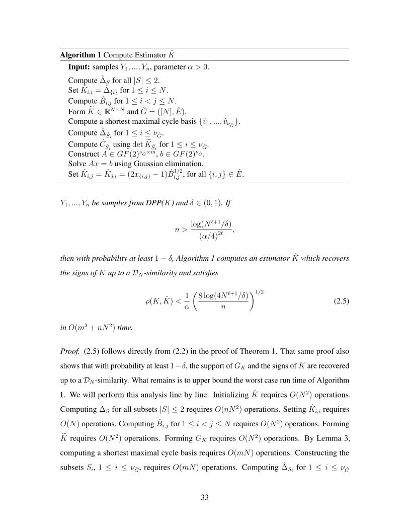
Algorithm 1 Compute Estimator Input: samples 𝑌1, ..., 𝑌𝑛, parameter 𝛼 > 0.

Compute ∆𝑆 for all |𝑆| ≤ 2.Set 𝑖,𝑖 = ∆𝑖 for 1 ≤ 𝑖 ≤ 𝑁 .Compute 𝑖,𝑗 for 1 ≤ 𝑖 < 𝑗 ≤ 𝑁 .Form 𝐾 ∈ R𝑁×𝑁 and = ([𝑁 ], ).Compute a shortest maximal cycle basis 𝑣1, ..., 𝑣𝜈.Compute ∆𝑆𝑖

for 1 ≤ 𝑖 ≤ 𝜈.Compute 𝐶𝑆𝑖

using det 𝐾𝑆𝑖for 1 ≤ 𝑖 ≤ 𝜈.

Construct 𝐴 ∈ 𝐺𝐹 (2)𝜈×𝑚, 𝑏 ∈ 𝐺𝐹 (2)𝜈 .Solve 𝐴𝑥 = 𝑏 using Gaussian elimination.Set 𝑖,𝑗 = 𝑗,𝑖 = (2𝑥𝑖,𝑗 − 1)

1/2𝑖,𝑗 , for all 𝑖, 𝑗 ∈ .

𝑌1, ..., 𝑌𝑛 be samples from DPP(𝐾) and 𝛿 ∈ (0, 1). If

𝑛 >log(𝑁 ℓ+1/𝛿)

(𝛼/4)2ℓ,

then with probability at least 1− 𝛿, Algorithm 1 computes an estimator which recovers

the signs of 𝐾 up to a 𝒟𝑁 -similarity and satisfies

𝜌(𝐾, ) <1

𝛼

(8 log(4𝑁 ℓ+1/𝛿)

𝑛

)1/2

(2.5)

in 𝑂(𝑚3 + 𝑛𝑁2) time.

Proof. (2.5) follows directly from (2.2) in the proof of Theorem 1. That same proof also

shows that with probability at least 1−𝛿, the support of 𝐺𝐾 and the signs of 𝐾 are recovered

up to a 𝒟𝑁 -similarity. What remains is to upper bound the worst case run time of Algorithm

1. We will perform this analysis line by line. Initializing requires 𝑂(𝑁2) operations.

Computing ∆𝑆 for all subsets |𝑆| ≤ 2 requires 𝑂(𝑛𝑁2) operations. Setting 𝑖,𝑖 requires

𝑂(𝑁) operations. Computing 𝑖,𝑗 for 1 ≤ 𝑖 < 𝑗 ≤ 𝑁 requires 𝑂(𝑁2) operations. Forming𝐾 requires 𝑂(𝑁2) operations. Forming 𝐺𝐾 requires 𝑂(𝑁2) operations. By Lemma 3,

computing a shortest maximal cycle basis requires 𝑂(𝑚𝑁) operations. Constructing the

subsets 𝑆𝑖, 1 ≤ 𝑖 ≤ 𝜈, requires 𝑂(𝑚𝑁) operations. Computing ∆𝑆𝑖for 1 ≤ 𝑖 ≤ 𝜈

33

requires 𝑂(𝑛𝑚) operations. Computing 𝐶𝑆𝑖using det( 𝐾[𝑆𝑖]) for 1 ≤ 𝑖 ≤ 𝜈 requires

𝑂(𝑚ℓ3) operations, where a factorization of each 𝐾[𝑆𝑖] is used to compute each determinant

in 𝑂(ℓ3) operations. Constructing 𝐴 and 𝑏 requires 𝑂(𝑚ℓ) operations. By Lemma 4, finding

a solution 𝑥 using Gaussian elimination requires 𝑂(𝑚3) operations. Setting 𝑖,𝑗 for all

edges 𝑖, 𝑗 ∈ 𝐸 requires 𝑂(𝑚) operations. Put this all together, Algorithm 1 runs in

𝑂(𝑚3 + 𝑛𝑁2) time.

Chordal Graphs

Here we show that it is possible to obtain faster algorithms by exploiting the structure

of 𝐺𝐾 . Specifically, in the case where 𝐺𝐾 chordal, we give an 𝑂(𝑚) time algorithm to

determine the signs of the off-diagonal entries of the estimator , resulting in an improved

overall runtime of 𝑂(𝑚 + 𝑛𝑁2). Recall that a graph 𝐺 = ([𝑁 ], 𝐸) is said to be chordal if

every induced cycle in 𝐺 is of length three. Moreover, a graph 𝐺 = ([𝑁 ], 𝐸) has a perfect

elimination ordering (PEO) if there exists an ordering of the vertex set 𝑣1, ..., 𝑣𝑁 such that,

for all 𝑖, the graph induced by 𝑣𝑖 ∪ 𝑣𝑗|𝑖, 𝑗 ∈ 𝐸, 𝑗 > 𝑖 is a clique. It is well known

that a graph is chordal if and only if it has a PEO. A PEO of a chordal graph with 𝑚 edges

can be computed in 𝑂(𝑚) operations using lexicographic breadth-first search [98].

Lemma 5. Let 𝐺 = ([𝑁 ], 𝐸), be a chordal graph and 𝑣1, ..., 𝑣𝑛 be a PEO. Given 𝑖,

let 𝑖* := min𝑗|𝑗 > 𝑖, 𝑣𝑖, 𝑣𝑗 ∈ 𝐸. Then the graph 𝐺′ = ([𝑁 ], 𝐸 ′), where 𝐸 ′ =

𝑣𝑖, 𝑣𝑖*𝑁−𝜅(𝐺)𝑖=1 , is a spanning forest of 𝐺.

Proof. We first show that there are no cycles in 𝐺′. Suppose to the contrary, that there is

an induced cycle 𝐶 of length 𝑘 on the vertices 𝑣𝑗1 , ..., 𝑣𝑗𝑘. Let 𝑣 be the vertex of smallest

index. Then 𝑣 is connected to two other vertices in the cycle of larger index. This is a

contradiction to the construction.

What remains is to show that |𝐸 ′| = 𝑁 − 𝜅(𝐺). It suffices to prove the case 𝜅(𝐺) = 1.

Suppose to the contrary, that there exists a vertex 𝑣𝑖, 𝑖 < 𝑁 , with no neighbors of larger

index. Let 𝑃 be the shortest path in 𝐺 from 𝑣𝑖 to 𝑣𝑁 . By connectivity, such a path exists.

Let 𝑣𝑘 be the vertex of smallest index in the path. However, it has two neighbors in the path

of larger index, which must be adjacent to each other. Therefore, there is a shorter path.

34

Algorithm 2 Compute Signs of Edges in Chordal Graph

Input: 𝐺𝐾 = ([𝑁 ], 𝐸) chordal, ∆𝑆 for |𝑆| ≤ 3.

Compute a perfect elimination ordering 𝑣1, ..., 𝑣𝑁.Compute the spanning forest 𝐺′ = ([𝑁 ], 𝐸 ′).Set all edges in 𝐸 ′ to have positive sign.Compute 𝐶𝑖,𝑗,𝑖* for all 𝑖, 𝑗 ∈ 𝐸 ∖ 𝐸 ′, 𝑗 < 𝑖.Order edges 𝐸 ∖ 𝐸 ′ = 𝑒1, ..., 𝑒𝜈 such that 𝑖 > 𝑗 if max 𝑒𝑖 < max 𝑒𝑗 .Visit edges in sorted order and for 𝑒 = 𝑖, 𝑗, 𝑗 > 𝑖, set

sgn(𝑖, 𝑗) = sgn(𝐶𝑖,𝑗,𝑖*) sgn(𝑖, 𝑖*) sgn(𝑗, 𝑖*).

Now, given the chordal graph 𝐺𝐾 induced by 𝐾 and the estimates of principal minors

of size at most three, we provide an algorithm to determine the signs of the edges of 𝐺𝐾 , or,

equivalently, the off-diagonal entries of 𝐾.

Theorem 4. If 𝐺𝐾 is chordal, Algorithm 2 correctly determines the signs of the edges of

𝐺𝐾 in 𝑂(𝑚) time.

Proof. We will simultaneously perform a count of the operations and a proof of the cor-

rectness of the algorithm. Computing a PEO requires 𝑂(𝑚) operations. Computing the

spanning forest requires 𝑂(𝑚) operations. The edges of the spanning tree can be given

arbitrary sign, because it is a cycle-free graph. This assigns a sign to two edges of each

3-cycle. Computing each 𝐶𝑖,𝑗,𝑖* requires a constant number of operations because ℓ = 3,

requiring a total of 𝑂(𝑚−𝑁) operations. Ordering the edges requires 𝑂(𝑚) operations.

Setting the signs of each remaining edge requires 𝑂(𝑚) operations.

Therefore, when 𝐺𝐾 is chordal, the overall complexity required by our algorithm to

compute is reduced to 𝑂(𝑚 + 𝑛𝑁2).

Experiments

Here we present experiments to supplement the theoretical results of the section. We test

our algorithm on two types of random matrices. First, we consider the matrix 𝐾 ∈ R𝑁×𝑁

35

(a) graph recovery, cycle (b) graph and sign recovery, cycle

(c) graph recovery, clique (d) graph and sign recovery, clique

Figure 2-1: Plots of the proportion of successive graph recovery, and graph and sign recovery,for random matrices with cycle and clique graph structure, respectively. The darker the box,the higher the proportion of trials that were recovered successfully.

corresponding to the cycle on 𝑁 vertices,

𝐾 =1

2𝐼 +

1

4𝐴,

where 𝐴 is symmetric and has non-zero entries only on the edges of the cycle, either +1 or

−1, each with probability 1/2. By the Gershgorin circle theorem, 0 ⪯ 𝐾 ⪯ 𝐼 . Next, we

consider the matrix 𝐾 ∈ R𝑁×𝑁 corresponding to the clique on 𝑁 vertices,

𝐾 =1

2𝐼 +

1

4√𝑁𝐴,

where 𝐴 is symmetric and has all entries either +1 or −1, each with probability 1/2. It is

well known that −2√𝑁 ⪯ 𝐴 ⪯ 2

√𝑁 with high probability, implying 0 ⪯ 𝐾 ⪯ 𝐼 .

For both cases and for a range of values of matrix dimension 𝑁 and samples 𝑛, we

run our algorithm on 50 randomly generated instances. We record the proportion of trials

where we recover the graph induced by 𝐾, and the proportion of the trials where we recover

36

both the graph and correctly determine the signs of the entries. In Figure 2-1, the shade of

each box represents the proportion of trials where recovery was successful for a given pair

𝑁, 𝑛. A completely white box corresponds to zero success rate, black to a perfect success

rate. The plots corresponding to the cycle and the clique are telling. We note that for the

clique, recovering the sparsity pattern and recovering the signs of the off-diagonal entries

come hand-in-hand. However, for the cycle, there is a noticeable gap between the number

of samples required to recover the sparsity pattern and the number of samples required to

recover the signs of the off-diagonal entries. This empirically confirms the central role that

cycle sparsity plays in parameter estimation, and further corroborates our theoretical results.

37

2.3 Recovering a Magnitude-Symmetric Matrix from its

Principal Minors

In this section, we consider matrices 𝐾 ∈ R𝑁×𝑁 satisfying |𝐾𝑖,𝑗| = |𝐾𝑗,𝑖| for 𝑖, 𝑗 ∈ [𝑁 ],

which we refer to as magnitude-symmetric matrices, and investigate the algorithmic question

of recovering such a matrix from its principal minors. First, we require a number of key

definitions and notation. For completeness (and to allow independent reading), we are

including terms and notations that we have defined in Section 2.2. If 𝐾 ∈ R𝑁×𝑁 and

𝑆 ⊆ [𝑁 ], 𝐾𝑆 := (𝐾𝑖,𝑗)𝑖,𝑗∈𝑆 and ∆𝑆(𝐾) := det𝐾𝑆 is the principal minor of 𝐾 associated

with the set 𝑆 (∆∅(𝐾) = 1 by convention). When it is clear from the context, we simply

write ∆𝑆 instead of ∆𝑆(𝐾), and for sets of order at most four, we replace the set itself by

its elements, i.e., write ∆1,2,3 as ∆1,2,3.

In addition, we recall a number of relevant graph-theoretic definitions. In this work, all

graphs 𝐺 are simple, undirected graphs. An articulation point or cut vertex of a graph 𝐺 is a

vertex whose removal disconnects the graph. A graph 𝐺 is said to be two-connected if it has

at least two vertices and has no articulation points. A maximal two-connected subgraph 𝐻

of 𝐺 is called a block of 𝐺. Given a graph 𝐺, a cycle 𝐶 is a subgraph of 𝐺 in which every

vertex of 𝐶 has even degree (within 𝐶). A simple cycle 𝐶 is a connected subgraph of 𝐺 in

which every vertex of 𝐶 has degree two. For simplicity, we may sometimes describe 𝐶 by a

traversal of its vertices along its edges, i.e., 𝐶 = 𝑖1 𝑖2 ... 𝑖𝑘 𝑖1; notice we have the choice of

the start vertex and the orientation of the cycle in this description. We denote the subgraph

induced by a vertex subset 𝑆 ⊂ 𝑉 by 𝐺[𝑆]. A simple cycle 𝐶 of a graph 𝐺 on vertex set

𝑉 (𝐶) is not necessarily induced, and while the cycle itself has all vertices of degree two,

this cycle may contain some number of chords in the original graph 𝐺, and we denote this

set 𝐸(𝐺[𝑆])∖𝐸(𝐶) of chords by 𝛾(𝐶).

Given any subgraph 𝐻 of 𝐺, we can associate with 𝐻 an incidence vector 𝜒𝐻 ∈ 𝐺𝐹 (2)𝑚,

𝑚 = |𝐸|, where 𝜒𝐻(𝑒) = 1 if and only if 𝑒 ∈ 𝐻 , and 𝜒𝐻(𝑒) = 0 otherwise. Given two

subgraphs 𝐻1, 𝐻2 ⊂ 𝐺 of 𝐺, we define their sum 𝐻1 + 𝐻2 as the graph containing all

edges in exactly one of 𝐸(𝐻1) and 𝐸(𝐻2) (i.e., their symmetric difference) and no isolated

38

vertices. This corresponds to the graph resulting from the sum of their incidence vectors.

The cycle space of 𝐺 is given by

𝒞(𝐺) = span𝜒𝐶 |𝐶 is a cycle of 𝐺 ⊂ 𝐺𝐹 (2)𝑚,

and has dimension 𝜈 = 𝑚 − 𝑁 + 𝜅(𝐺), where 𝜅(𝐺) denotes the number of connected

components of 𝐺. The quantity 𝜈 is commonly referred to as the cyclomatic number. The

cycle sparsity ℓ of the graph 𝐺 is the smallest number for which the set of incidence vectors

𝜒𝐶 of cycles of edge length at most ℓ spans 𝒞(𝐺).

In this section, we require the use and analysis of graphs 𝐺 = ([𝑁 ], 𝐸) endowed with a

linear Boolean function 𝜖 that maps subgraphs of 𝐺 to −1,+1, i.e., 𝜖(𝑒) ∈ −1,+1 for

all 𝑒 ∈ 𝐸(𝐺) and

𝜖(𝐻) =∏

𝑒∈𝐸(𝐻)

𝜖(𝑒)

for all subgraphs 𝐻 . The graph 𝐺 combined with a linear Boolean function 𝜖 is denoted

by 𝐺 = ([𝑁 ], 𝐸, 𝜖) and referred to as a charged graph. If 𝜖(𝐻) = +1 (resp. 𝜖(𝐻) = −1),

then we say the subgraph 𝐻 is positive (resp. negative). For the sake of space, we often

denote 𝜖(𝑖, 𝑗), 𝑖, 𝑗 ∈ 𝐸(𝐺), by 𝜖𝑖,𝑗 . Given a magnitude-symmetric matrix 𝐾 ∈ R𝑁×𝑁 ,

|𝐾𝑖,𝑗| = |𝐾𝑗,𝑖| for 𝑖, 𝑗 ∈ [𝑁 ], we define the charged sparsity graph 𝐺𝐾 as 𝐺𝐾 = ([𝑁 ], 𝐸, 𝜖),

𝐸 := 𝑖, 𝑗 ∈ [𝑁 ] | 𝑖 = 𝑗, |𝐾𝑖,𝑗| = 0, 𝜖(𝑖, 𝑗) := sgn(𝐾𝑖,𝑗𝐾𝑗,𝑖), and when clear from

context, we simply write 𝐺 instead of 𝐺𝐾 .

We define the span of the incidence vectors of positive cycles as

𝒞+(𝐺) = span𝜒𝐶 |𝐶 is a cycle of 𝐺, 𝜖(𝐶) = +1.

As we will see, when 𝐻 is a block, the space 𝒞+(𝐻) is spanned by positive simple cycles

(Proposition 3). We define the simple cycle sparsity ℓ+ of 𝒞+(𝐺) to be the smallest number

for which the set of incidence vectors 𝜒𝐶 of positive simple cycles of edge length at most

ℓ+ spans 𝒞+(𝐺) (or, equivalently, the set 𝒞+(𝐻) for every block 𝐻 of 𝐺). Unlike 𝒞(𝐺), for

𝒞+(𝐺) this quantity ℓ+ depends on whether we consider a basis of cycles or of only simple

39

cycles. The study of bases of 𝒞+(𝐻), for blocks 𝐻 , consisting of incidence vectors of simple

cycles constitutes the major graph-theoretic subject of this work, and has connections to the

recovery of a magnitude-symmetric matrix from its principal minors.

2.3.1 Principal Minors and Magnitude-Symmetric Matrices

In this subsection, we are primarily concerned with recovering a magnitude-symmetric

matrix 𝐾 from its principal minors. Using only principal minors of order one and two,

the quantities 𝐾𝑖,𝑖, 𝐾𝑖,𝑗𝐾𝑗,𝑖, and the charged graph 𝐺𝐾 can be computed immediately, as

𝐾𝑖,𝑖 = ∆𝑖 and 𝐾𝑖,𝑗𝐾𝑗,𝑖 = ∆𝑖∆𝑗 −∆𝑖,𝑗 for all 𝑖 = 𝑗. The main focus of this subsection is

to obtain further information on 𝐾 using principal minors of order greater than two, and

to quantify the extent to which 𝐾 can be identified from its principal minors. To avoid the

unintended cancellation of terms in a principal minor, in what follows we assume that 𝐾 is

generic in the sense that

If 𝐾𝑖,𝑗𝐾𝑗,𝑘𝐾𝑘,ℓ𝐾ℓ,𝑖 = 0 for 𝑖, 𝑗, 𝑘, ℓ ∈ [𝑁 ] distinct, then |𝐾𝑖,𝑗𝐾𝑘,ℓ| = |𝐾𝑗,𝑘𝐾ℓ,𝑖|, (2.6)

and 𝜑1𝐾𝑖,𝑗𝐾𝑗,𝑘𝐾𝑘,ℓ𝐾ℓ,𝑖 + 𝜑2𝐾𝑖,𝑗𝐾𝑗,ℓ𝐾ℓ,𝑘𝐾𝑘,𝑖 + 𝜑3𝐾𝑖,𝑘𝐾𝑘,𝑗𝐾𝑗,ℓ𝐾ℓ,𝑖 = 0

for all 𝜑1, 𝜑2, 𝜑3 ∈ −1, 1.

The first part of the condition in (2.6) implies that the three terms (corresponding to the three

distinct cycles on 4 vertices) in the second part are all distinct in magnitude; the second

part strengthens this requirement. Condition (2.6) can be thought of as a no-cancellation

requirement for four-cycles of principal minors of order four. As we will see, this condition

is quite important for the recovery of a magnitude-symmetric matrix from its principal

minors. Though, the results of this section, slightly modified, hold under slightly weaker

conditions than (2.6), albeit at the cost of simplicity. This condition rules out dense matrices

with a high degree of symmetry, as well as the large majority of rank one matrices, but this

condition is satisfied for almost all matrices.

We denote the set of 𝑁 ×𝑁 magnitude-symmetric matrices satisfying Property (2.6)

by 𝒦𝑁 , and, when the dimension is clear from context, we often simply write 𝒦. We note

40

that if 𝐾 ∈ 𝒦, then any matrix 𝐾 ′ satisfying |𝐾 ′𝑖,𝑗| = |𝐾𝑖,𝑗|, 𝑖, 𝑗 ∈ [𝑁 ], is also in 𝒦. In this

subsection, we answer the following question:

Given 𝐾 ∈ 𝒦, what is the minimal ℓ+ such that any 𝐾 ′ ∈ 𝒦 with (2.7)

∆𝑆(𝐾) = ∆𝑆(𝐾 ′) for all |𝑆| ≤ ℓ+ also satisfies ∆𝑆(𝐾) = ∆𝑆(𝐾 ′)

for all 𝑆 ⊂ [𝑁 ]?

Question (2.7) asks for the smallest ℓ such that the principal minors of order at most ℓ

uniquely determines principal minors of all orders. In Theorem 5, we show that the answer

is the simple cycle sparsity of 𝒞+(𝐺). In Subsections 2.3.2 and 2.3.3, we build on the

analysis of this subsection, and produce a polynomial-time algorithm for recovering a matrix

𝐾 with prescribed principal minors (possibly given up to some error term). The polynomial-

time algorithm (of Subsection 2.3.3) for recovery given perturbed principal minors has key

connections to learning signed DPPs.

In addition, it is also reasonable to ask:

Given 𝐾 ∈ 𝒦, what is the set of 𝐾 ′ ∈ 𝒦 that satisfy ∆𝑆(𝐾) = ∆𝑆(𝐾 ′) (2.8)

for all 𝑆 ⊂ [𝑁 ]?

Question (2.8) treats the extent to which we can hope to recover a matrix from its principal

minors. For instance, the transpose operation 𝐾𝑇 and the similarity transformation 𝐷𝐾𝐷,

where 𝐷 is a diagonal matrix with entries −1,+1 on the diagonal, both clearly preserve

principal minors. In fact, these two operations suitably combined completely define this

set. This result follows fairly quickly from a more general result of Loewy [79, Theorem 1]

regarding matrices with all principal minors equal. In particular, Loewy shows that if two

𝑛× 𝑛, 𝑛 ≥ 4, matrices 𝐴 and 𝐵 have all principal minors equal, and 𝐴 is irreducible and

rank(𝐴𝑆,𝑇 ) ≥ 2 or rank(𝐴𝑇,𝑆) ≥ 2 (where 𝐴𝑆,𝑇 is the submatrix of 𝐴 containing the rows

in 𝑆 and the columns in 𝑇 ) for all partitions 𝑆 ∪ 𝑇 = [𝑛], 𝑆 ∩ 𝑇 = ∅, |𝑆|, |𝑇 | ≥ 2, then

either 𝐵 or 𝐵𝑇 is diagonally similar to 𝐴. In Proposition 4, we include an alternate proof

41

answering Question (2.8), as Loewy’s result and proof, though more general and quite nice,

is more involved and not as illuminating for the specific case that we consider here.

To answer Question (2.7), we study properties of certain bases of the space 𝒞+(𝐺). We

recall that, given a matrix 𝐾 ∈ 𝒦, we can define the charged sparsity graph 𝐺 = ([𝑁 ], 𝐸, 𝜖)

of 𝐾, where 𝐺 is the simple graph on vertex set [𝑁 ] with an edge 𝑖, 𝑗 ∈ 𝐸, 𝑖 = 𝑗, if

𝐾𝑖,𝑗 = 0 and endowed with a function 𝜖 mapping subgraphs of 𝐺 to −1,+1. Viewing the

possible values ±1 for 𝜖 as the two elements of 𝐺𝐹 (2), we note that 𝜖(𝐻) is additive over

𝐺𝐹 (2), i.e. 𝜖(𝐻1 + 𝐻2) = 𝜖(𝐻1)𝜖(𝐻2). We can make a number of observations regarding

the connectivity of 𝐺. If 𝐺 is disconnected, with connected components given by vertex

sets 𝑉1, ..., 𝑉𝑘, then any principal minor ∆𝑆 satisfies

∆𝑆 =𝑘∏

𝑗=1

∆𝑆∩𝑉𝑗. (2.9)

In addition, if 𝐺 has a cut vertex 𝑖, whose removal results in connected components with

vertex sets 𝑉1, ..., 𝑉𝑘, then the principal minor ∆𝑆 satisfies

∆𝑆 =𝑘∑

𝑗1=1

∆[𝑖∪𝑉𝑗1]∩𝑆

∏𝑗2 =𝑗1

∆𝑉𝑗2∩𝑆 − (𝑘 − 1)∆𝑖∩𝑆

𝑘∏𝑗=1

∆𝑉𝑗∩𝑆. (2.10)

This implies that the principal minors of 𝐾 are uniquely determined by principal minors

corresponding to subsets of blocks of 𝐺. Given this property, we focus on matrices 𝐾

without an articulation point, i.e. 𝐺 is two-connected. Given results for matrices without an

articulation point and Equations (2.9) and (2.10), we can then answer Question (2.7) in the

more general case.

Next, we make an important observation regarding the contribution of certain terms

in the Laplace expansion of a principal minor. Recall that the Laplace expansion of the

determinant is given by

det(𝐾) =∑𝜎∈𝒮𝑁

sgn(𝜎)𝑁∏𝑖=1

𝐾𝑖,𝜎(𝑖),

42

where sgn(𝜎) is multiplicative over the (disjoint) cycles forming the permutation, and is

preserved when taking the inverse of the permutation, or of any cycle therein. Consider

now an arbitrary, possibly non-induced, simple cycle 𝐶 (in the graph-theoretic sense) of

the sparsity graph 𝐺, without loss of generality given by 𝐶 = 1 2 ... 𝑘 1, that satisfies

𝜖(𝐶) = −1. Consider the sum of all terms in the Laplace expansion that contains either

the cycle (1 2 ... 𝑘) or its inverse (𝑘 𝑘 − 1 ... 1) in the associated permutation. Because

𝜖(𝐶) = −1,

𝐾𝑘,1

𝑘−1∏𝑖=1

𝐾𝑖,𝑖+1 + 𝐾1,𝑘

𝑘∏𝑖=2

𝐾𝑖,𝑖−1 = 0,

and the sum over all permutations containing the cyclic permutations (𝑘 𝑘 − 1 ... 1) or

(1 2 ... 𝑘) is zero. Therefore, terms associated with permutations containing negative cycles

(𝜖(𝐶) = −1) do not contribute to principal minors.

To illustrate the additional information contained in higher order principal minors ∆𝑆 ,

|𝑆| > 2, we first consider principal minors of order three and four. Consider the principal

minor ∆1,2,3, given by

∆1,2,3 = 𝐾1,1𝐾2,2𝐾3,3 −𝐾1,1𝐾2,3𝐾3,2 −𝐾2,2𝐾1,3𝐾3,1 −𝐾3,3𝐾1,2𝐾2,1

+ 𝐾1,2𝐾2,3𝐾3,1 + 𝐾3,2𝐾2,1𝐾1,3

= ∆1∆2∆3 −∆1

[∆2∆3 −∆2,3

]−∆2

[∆1∆3 −∆1,3

]−∆3

[∆1∆2 −∆1,2

]+[1 + 𝜖1,2𝜖2,3𝜖3,1

]𝐾1,2𝐾2,3𝐾3,1.

If the corresponding graph 𝐺[1, 2, 3] is not a cycle, or if the cycle is negative (𝜖1,2𝜖2,3𝜖3,1 =

−1), then ∆1,2,3 can be written in terms of principal minors of order at most two, and contains

no additional information about 𝐾. If 𝐺[1, 2, 3] is a positive cycle, then we can write

𝐾1,2𝐾2,3𝐾3,1 as a function of principal minors of order at most three,

𝐾1,2𝐾2,3𝐾3,1 = ∆1∆2∆3 −1

2

[∆1∆2,3 + ∆2∆1,3 + ∆3∆1,2

]+

1

2∆1,2,3,

which allows us to compute sgn(𝐾1,2𝐾2,3𝐾3,1). This same procedure holds for any posi-

tively charged induced simple cycle in 𝐺. However, when a simple cycle is not induced,

43

further analysis is required. To illustrate some of the potential issues for a non-induced

positive simple cycle, we consider principal minors of order four.

Consider the principal minor ∆1,2,3,4. By our previous analysis, all terms in the Laplace

expansion of ∆1,2,3,4 corresponding to permutations with cycles of length at most three can

be written in terms of principal minors of size at most three. What remains is to consider

the sum of the terms in the Laplace expansion corresponding to permutations containing

a cycle of length four (which there are three pairs of, each pair corresponding to the two

orientations of a cycle of length four in the graph sense), which we denote by 𝑍, given by

𝑍 = −𝐾1,2𝐾2,3𝐾3,4𝐾4,1 −𝐾1,2𝐾2,4𝐾4,3𝐾3,1 −𝐾1,3𝐾3,2𝐾2,4𝐾4,1

−𝐾4,3𝐾3,2𝐾2,1𝐾1,4 −𝐾4,2𝐾2,1𝐾1,3𝐾3,4 −𝐾4,2𝐾2,3𝐾3,1𝐾1,4.

If 𝐺[1, 2, 3, 4] does not contain a positive simple cycle of length four, then 𝑍 = 0 and

∆1,2,3,4 can be written in terms of principal minors of order at most three. If 𝐺[1, 2, 3, 4]

has exactly one positive cycle of length four, without loss of generality given by 𝐶 :=

1 2 3 4 1, then

𝑍 = −[1 + 𝜖(𝐶)

]𝐾1,2𝐾2,3𝐾3,4𝐾4,1 = −2𝐾1,2𝐾2,3𝐾3,4𝐾4,1,

and we can write 𝐾1,2𝐾2,3𝐾3,4𝐾4,1 as a function of principal minors of order at most four,

which allows us to compute sgn(𝐾1,2𝐾2,3𝐾3,4𝐾4,1). Finally, we treat the case in which

there is more than one positive simple cycle of length four. This implies that all simple

cycles of length four are positive and 𝑍 is given by

𝑍 = −2[𝐾1,2𝐾2,3𝐾3,4𝐾4,1 + 𝐾1,2𝐾2,4𝐾4,3𝐾3,1 + 𝐾1,3𝐾3,2𝐾2,4𝐾4,1

]. (2.11)

By Condition (2.6), the magnitude of each of these three terms is distinct, 𝑍 = 0, and we can

compute the sign of each of these terms, as there is a unique choice of 𝜑1, 𝜑2, 𝜑3 ∈ −1,+1

44

satisfying

𝜑1|𝐾1,2𝐾2,3𝐾3,4𝐾4,1|+ 𝜑2|𝐾1,2𝐾2,4𝐾4,3𝐾3,1|+ 𝜑3|𝐾1,3𝐾3,2𝐾2,4𝐾4,1| = −𝑍

2.

In order to better understand the behavior of principal minors of order greater than four, we

investigate the set of positive simple cycles (i.e., simple cycles 𝐶 satisfying 𝜖(𝐶) = +1). In

the following two propositions, we compute the dimension of 𝒞+(𝐺), and note that when

𝐺 is two-connected, this space is spanned by incidence vectors corresponding to positive

simple cycles.

Proposition 2. Let 𝐺 = ([𝑁 ], 𝐸, 𝜖) be a charged graph. Then dim(𝒞+(𝐺)) = 𝜈 − 1 if 𝐺

contains at least one negative cycle, and equals 𝜈 otherwise.

Proof. Consider a basis 𝑥1, ..., 𝑥𝜈 for 𝒞(𝐺). If all associated cycles are positive, then

dim(𝒞+(𝐺)) = 𝜈 and we are done. If 𝐺 has a negative cycle, then, by the linearity of 𝜖, at

least one element of 𝑥1, ..., 𝑥𝜈 must be the incidence vector of a negative cycle. Without

loss of generality, suppose that 𝑥1, ..., 𝑥𝑖 are incidence vectors of negative cycles. Then

𝑥1 + 𝑥2, ..., 𝑥1 + 𝑥𝑖, 𝑥𝑖+1, ..., 𝑥𝜈 is a linearly independent set of incidence vectors of positive

cycles. Therefore, dim(𝒞+(𝐺)) ≥ 𝜈 − 1. However, 𝑥1 is the incidence vector of a negative

cycle, and so cannot be in the span of 𝑥1 + 𝑥2, ..., 𝑥1 + 𝑥𝑖, 𝑥𝑖+1, ..., 𝑥𝜈 .

Proposition 3. Let 𝐺 = ([𝑁 ], 𝐸, 𝜖) be a two-connected charged graph. Then

𝒞+(𝐺) = span𝜒𝐶 |𝐶 is a simple cycle of 𝐺, 𝜖(𝐶) = +1.

Proof. If 𝐺 does not contain a negative cycle, then the result follows immediately, as then

𝒞+(𝐺) = 𝒞(𝐺). Suppose then that 𝐺 has at least one negative cycle. Decomposing this

negative cycle into the union of edge-disjoint simple cycles, we note that 𝐺 must also have

at least one negative simple cycle.

Since 𝐺 is a two-connected graph, it admits a proper (also called open) ear decomposition

with 𝜈 − 1 proper ears (Whitney [128], see also [63]) starting from any simple cycle. We

choose our initial simple cycle to be a negative simple cycle denoted by 𝐺0. Whitney’s proper

45

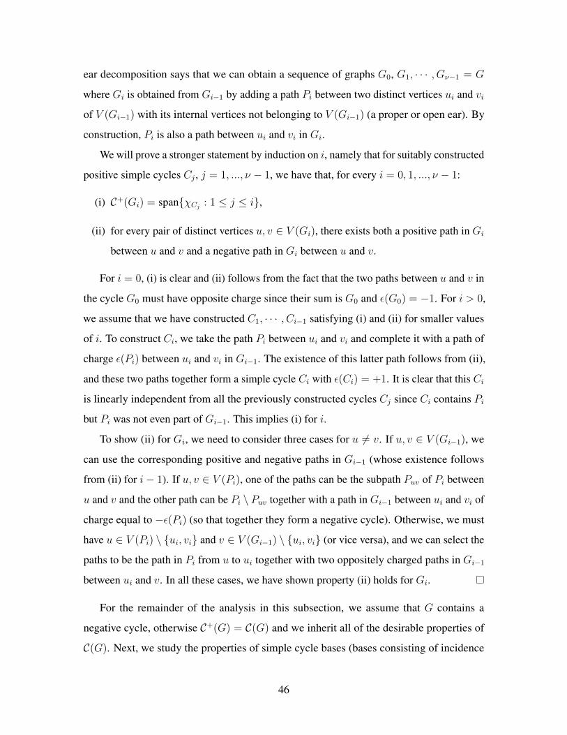
ear decomposition says that we can obtain a sequence of graphs 𝐺0, 𝐺1, · · · , 𝐺𝜈−1 = 𝐺

where 𝐺𝑖 is obtained from 𝐺𝑖−1 by adding a path 𝑃𝑖 between two distinct vertices 𝑢𝑖 and 𝑣𝑖

of 𝑉 (𝐺𝑖−1) with its internal vertices not belonging to 𝑉 (𝐺𝑖−1) (a proper or open ear). By

construction, 𝑃𝑖 is also a path between 𝑢𝑖 and 𝑣𝑖 in 𝐺𝑖.

We will prove a stronger statement by induction on 𝑖, namely that for suitably constructed

positive simple cycles 𝐶𝑗 , 𝑗 = 1, ..., 𝜈 − 1, we have that, for every 𝑖 = 0, 1, ..., 𝜈 − 1:

(i) 𝒞+(𝐺𝑖) = span𝜒𝐶𝑗: 1 ≤ 𝑗 ≤ 𝑖,

(ii) for every pair of distinct vertices 𝑢, 𝑣 ∈ 𝑉 (𝐺𝑖), there exists both a positive path in 𝐺𝑖

between 𝑢 and 𝑣 and a negative path in 𝐺𝑖 between 𝑢 and 𝑣.

For 𝑖 = 0, (i) is clear and (ii) follows from the fact that the two paths between 𝑢 and 𝑣 in

the cycle 𝐺0 must have opposite charge since their sum is 𝐺0 and 𝜖(𝐺0) = −1. For 𝑖 > 0,

we assume that we have constructed 𝐶1, · · · , 𝐶𝑖−1 satisfying (i) and (ii) for smaller values

of 𝑖. To construct 𝐶𝑖, we take the path 𝑃𝑖 between 𝑢𝑖 and 𝑣𝑖 and complete it with a path of

charge 𝜖(𝑃𝑖) between 𝑢𝑖 and 𝑣𝑖 in 𝐺𝑖−1. The existence of this latter path follows from (ii),

and these two paths together form a simple cycle 𝐶𝑖 with 𝜖(𝐶𝑖) = +1. It is clear that this 𝐶𝑖

is linearly independent from all the previously constructed cycles 𝐶𝑗 since 𝐶𝑖 contains 𝑃𝑖

but 𝑃𝑖 was not even part of 𝐺𝑖−1. This implies (i) for 𝑖.

To show (ii) for 𝐺𝑖, we need to consider three cases for 𝑢 = 𝑣. If 𝑢, 𝑣 ∈ 𝑉 (𝐺𝑖−1), we

can use the corresponding positive and negative paths in 𝐺𝑖−1 (whose existence follows

from (ii) for 𝑖− 1). If 𝑢, 𝑣 ∈ 𝑉 (𝑃𝑖), one of the paths can be the subpath 𝑃𝑢𝑣 of 𝑃𝑖 between

𝑢 and 𝑣 and the other path can be 𝑃𝑖 ∖ 𝑃𝑢𝑣 together with a path in 𝐺𝑖−1 between 𝑢𝑖 and 𝑣𝑖 of

charge equal to −𝜖(𝑃𝑖) (so that together they form a negative cycle). Otherwise, we must

have 𝑢 ∈ 𝑉 (𝑃𝑖) ∖ 𝑢𝑖, 𝑣𝑖 and 𝑣 ∈ 𝑉 (𝐺𝑖−1) ∖ 𝑢𝑖, 𝑣𝑖 (or vice versa), and we can select the

paths to be the path in 𝑃𝑖 from 𝑢 to 𝑢𝑖 together with two oppositely charged paths in 𝐺𝑖−1

between 𝑢𝑖 and 𝑣. In all these cases, we have shown property (ii) holds for 𝐺𝑖.

For the remainder of the analysis in this subsection, we assume that 𝐺 contains a

negative cycle, otherwise 𝒞+(𝐺) = 𝒞(𝐺) and we inherit all of the desirable properties of

𝒞(𝐺). Next, we study the properties of simple cycle bases (bases consisting of incidence

46

vectors of simple cycles) of 𝒞+(𝐺) that are minimal in some sense. We say that a simple

cycle basis 𝜒𝐶1 , ..., 𝜒𝐶𝜈−1 for 𝒞+(𝐺) is lexicographically minimal if it lexicographically

minimizes (|𝐶1|, |𝐶2|, ..., |𝐶𝜈−1|), i.e., minimizes |𝐶1|, minimizes |𝐶2| conditional on |𝐶1|

being minimal, etc. Any lexicographical minimal basis also minimizes∑|𝐶𝑖| and max |𝐶𝑖|

(by optimality of the greedy algorithm for (linear) matroids). For brevity, we will simply

refer to such a basis as “minimal." One complicating issue is that, while a minimal cycle

basis for 𝒞(𝐺) always consists of induced simple cycles, this is no longer the case for 𝒞+(𝐺).

This for example can happen for an appropriately constructed graph with only two negative,

short simple cycles, far away from each other; a minimal cycle basis for 𝒞+(𝐺) then contains

a cycle consisting of the union of these 2 negative simple cycles.

However, we can make a number of statements regarding chords of simple cycles

corresponding to elements of a minimal simple cycle basis of 𝒞+(𝐺). In the following

lemma, we show that a minimal simple cycle basis satisfies a number of desirable properties.

However, before we do so, we introduce some useful notation. Given a simple cycle 𝐶, it is

convenient to fix an orientation say 𝐶 = 𝑖1 𝑖2 ... 𝑖𝑘 𝑖1. Now for any chord 𝑖𝑘1 , 𝑖𝑘2 ∈ 𝛾(𝐶),

𝑘1 < 𝑘2, we denote the two cycles created by this chord by

𝐶(𝑘1, 𝑘2) = 𝑖𝑘1 𝑖𝑘1+1 ... 𝑖𝑘2 𝑖𝑘1 and 𝐶(𝑘2, 𝑘1) = 𝑖𝑘2 𝑖𝑘2+1 ... 𝑖𝑘 𝑖1 ... 𝑖𝑘1 𝑖𝑘2 .

We have the following result.

Lemma 6. Let 𝐺 = ([𝑁 ], 𝐸, 𝜖) be a two-connected charged graph, and 𝐶 := 𝑖1 𝑖2 ... 𝑖𝑘 𝑖1

be a cycle corresponding to an incidence vector of a minimal simple cycle basis 𝑥1, ..., 𝑥𝜈−1

of 𝒞+(𝐺). Then

(i) 𝜖(𝐶(𝑘1, 𝑘2)

)= 𝜖(𝐶(𝑘2, 𝑘1)

)= −1 for all 𝑖𝑘1 , 𝑖𝑘2 ∈ 𝛾(𝐶),

(ii) if 𝑖𝑘1 , 𝑖𝑘2, 𝑖𝑘3 , 𝑖𝑘4 ∈ 𝛾(𝐶) satisfy 𝑘1 < 𝑘3 < 𝑘2 < 𝑘4 (crossing chords), then either

𝑘3 − 𝑘1 = 𝑘4 − 𝑘2 = 1 or 𝑘1 = 1, 𝑘2 − 𝑘3 = 1, 𝑘4 = 𝑘, i.e. these two chords form a

four-cycle with two edges of the cycle,

(iii) there does not exist 𝑖𝑘1 , 𝑖𝑘2, 𝑖𝑘3 , 𝑖𝑘4, 𝑖𝑘5 , 𝑖𝑘6 ∈ 𝛾(𝐶) satisfying either 𝑘1 < 𝑘2 ≤

47

𝑘3 < 𝑘4 ≤ 𝑘5 < 𝑘6 or 𝑘6 ≤ 𝑘1 < 𝑘2 ≤ 𝑘3 < 𝑘4 ≤ 𝑘5.

Proof. Without loss of generality, suppose that 𝐶 = 1 2 ... 𝑘. Given a chord 𝑘1, 𝑘2,

𝐶(𝑘1, 𝑘2) + 𝐶(𝑘2, 𝑘1) = 𝐶, and so 𝜖(𝐶) = +1 implies that 𝜖(𝐶(𝑘1, 𝑘2)

)= 𝜖(𝐶(𝑘2, 𝑘1)

).

If both these cycles were positive, then this would contradict the minimality of the basis, as

|𝐶(𝑘1, 𝑘2)|, |𝐶(𝑘2, 𝑘1)| < 𝑘. This completes the proof of Property (i).

Given two chords 𝑘1, 𝑘2 and 𝑘3, 𝑘4 satisfying 𝑘1 < 𝑘3 < 𝑘2 < 𝑘4, we consider the

cycles

𝐶1 := 𝐶(𝑘1, 𝑘2) + 𝐶(𝑘3, 𝑘4),

𝐶2 := 𝐶(𝑘1, 𝑘2) + 𝐶(𝑘4, 𝑘3).

By Property (i), 𝜖(𝐶1) = 𝜖(𝐶2) = +1. In addition, 𝐶1 + 𝐶2 = 𝐶, and |𝐶1|, |𝐶2| ≤ |𝐶|.

By the minimality of the basis, either |𝐶1| = |𝐶| or |𝐶2| = |𝐶|, which implies that either

|𝐶1| = 4 or |𝐶2| = 4 (or both). This completes the proof of Property (ii).

Given three non-crossing chords 𝑘1, 𝑘2, 𝑘3, 𝑘4, and 𝑘5, 𝑘6, with 𝑘1 < 𝑘2 ≤ 𝑘3 <

𝑘4 ≤ 𝑘5 < 𝑘6 (the other case is identical, up to rotation), we consider the cycles

𝐶1 := 𝐶(𝑘3, 𝑘4) + 𝐶(𝑘5, 𝑘6) + 𝐶,

𝐶2 := 𝐶(𝑘1, 𝑘2) + 𝐶(𝑘5, 𝑘6) + 𝐶,

𝐶3 := 𝐶(𝑘1, 𝑘2) + 𝐶(𝑘3, 𝑘4) + 𝐶.

By Property (i), 𝜖(𝐶1) = 𝜖(𝐶2) = 𝜖(𝐶3) = +1. In addition, 𝐶1 + 𝐶2 + 𝐶3 = 𝐶 and

|𝐶1|, |𝐶2|, |𝐶3| < |𝐶|, a contradiction to the minimality of the basis. This completes the

proof of Property (iii).

The above lemma tells us that in a minimal simple cycle basis for 𝒞+(𝐺), in each cycle

two crossing chords always form a positive cycle of length four (and thus any chord has at

most one other crossing chord), and there doesn’t exist three non-crossing chords without

one chord in between the other two. Using a simple cycle basis of 𝒞+(𝐺) that satisfies the

three properties of the above lemma, we aim to show that the principal minors of order at

48

most the length of the longest cycle in the basis uniquely determine the principal minors of

all orders. To do so, we prove a series of three lemmas that show that from the principal

minor corresponding to a cycle 𝐶 = 𝑖1 ... 𝑖𝑘 𝑖1 in our basis and 𝑂(1) principal minors of

subsets of 𝑉 (𝐶), we can compute the quantity

𝑠(𝐶) :=∏

𝑖,𝑗∈𝐸(𝐶),𝑖<𝑗

sgn(𝐾𝑖,𝑗

).

Once we have computed 𝑠(𝐶𝑖) for every simple cycle in our basis, we can compute 𝑠(𝐶)

for any simple positive cycle by writing 𝐶 as a sum of some subset of the simple cycles

𝐶1, ..., 𝐶𝜈−1 corresponding to incidence vectors in our basis, and taking the product of 𝑠(𝐶𝑖)

for all indices 𝑖 in the aforementioned sum. To this end, we prove the following three

lemmas.

Lemma 7. Let 𝐶 be a positive simple cycle of 𝐺 = ([𝑁 ], 𝐸, 𝜖) with 𝑉 (𝐶) = 𝑖1, 𝑖2, · · · , 𝑖𝑘

whose chords 𝛾(𝐶) satisfy Properties (i)-(iii) of Lemma 6. Then there exist two edges of 𝐶,

say, 𝑖1, 𝑖𝑘 and 𝑖ℓ, 𝑖ℓ+1, where 𝐶 := 𝑖1 𝑖2 ... 𝑖𝑘 𝑖1 such that

(i) all chords 𝑖𝑝, 𝑖𝑞 ∈ 𝛾(𝐶), 𝑝 < 𝑞, satisfy 𝑝 ≤ ℓ < 𝑞,

(ii) any positive simple cycle in 𝐺[𝑉 (𝐶)] containing 𝑖1, 𝑖𝑘 spans 𝑉 (𝐶) and contains

only edges in 𝐸(𝐶) and pairs of crossed chords.

Proof. We first note that Property (i) of Lemma 6 implies that the charge of a cycle 𝐶 ′ ⊂

𝐺[𝑉 (𝐶)] corresponds to the parity of 𝐸(𝐶 ′) ∩ 𝛾(𝐶), i.e., if 𝐶 ′ contains an even number of

chords then 𝜖(𝐶 ′) = +1, otherwise 𝜖(𝐶 ′) = −1. This follows from constructing a cycle

basis for 𝐺[𝑉 (𝐶)] consisting of incidence vectors corresponding to 𝐶 and 𝐶(𝑢, 𝑣) for every

chord 𝑢, 𝑣 ∈ 𝛾(𝐶).

Let the cycle 𝐶(𝑖, 𝑗) be a shortest cycle in 𝐺[𝑉 (𝐶)] containing exactly one chord of

𝐶. If this is a non-crossed chord, then we take an arbitrary edge in 𝐸(𝐶(𝑖, 𝑗))∖𝑖, 𝑗 to be

𝑖1, 𝑖𝑘. If this chord crosses another, denoted by 𝑖′, 𝑗′, then either 𝐶(𝑖′, 𝑗′) or 𝐶(𝑗′, 𝑖′) is

also a shortest cycle, and we take an arbitrary edge in the intersection of these two shortest

49

cycles. Without loss of generality, let 1, 𝑘 denote this edge and let the cycle be 1 2 ... 𝑘 1,

where for simplicity we have assumed that 𝑉 (𝐶) = [𝑘]. Because of Property (iii) of Lemma

6, there exists ℓ such that all chords 𝑖, 𝑗 ∈ 𝛾(𝐶) satisfy 𝑖 ≤ ℓ and 𝑗 > ℓ. This completes

the proof of Property (i).

Next, consider an arbitrary positive simple cycle 𝐶 ′ in 𝐺[𝑉 (𝐶)] containing 1, 𝑘.

We aim to show that this cycle contains only edges in 𝐸(𝐺) and pairs of crossed chords,

from which the equality 𝑉 (𝐶 ′) = 𝑉 (𝐶) immediately follows. Since 𝐶 ′ is positive, it

contains an even number of chords 𝛾(𝐶), and either all the chords 𝛾(𝐶) ∩ 𝐸(𝐶 ′) are pairs

of crossed chords or there exist two chords 𝑝1, 𝑞1, 𝑝2, 𝑞2 ∈ 𝛾(𝐶) ∩ 𝐸(𝐶 ′), w.l.o.g.

𝑝1 ≤ 𝑝2 ≤ ℓ < 𝑞2 < 𝑞1 (we can simply reverse the orientation if 𝑞1 = 𝑞2), that do not cross

any other chord in 𝛾(𝐶) ∩ 𝐸(𝐶 ′). In this case, there would be a 1− 𝑞2 path in 𝐶 ′ neither

containing 𝑝1 nor 𝑞1 (as 𝑝1, 𝑞1 would be along the other path between 1 and 𝑞2 in 𝐶 ′ and

𝑞1 = 𝑞2). However, this is a contradiction as no such path exists in 𝐶 ′, since 𝑝1, 𝑞1 does

not cross any chord in 𝛾(𝐶) ∩ 𝐸(𝐶 ′). Therefore, the chords 𝛾(𝐶) ∩ 𝐸(𝐶 ′) are all pairs of

crossed chords. Furthermore, since all pairs of crossed chords must define cycles of length

4, we have 𝑉 (𝐶 ′) = 𝑉 (𝐶). This completes the proof of Property (ii).

Although this is not needed in what follows, observe that, in the above Lemma 7,

𝑖ℓ, 𝑖ℓ+1 also plays the same role as 𝑖1, 𝑖𝑘 in the sense that any positive simple cycle

containing 𝑖ℓ, 𝑖ℓ+1 also spans 𝑉 (𝐶) and contains only pairs of crossed chords and edges

in 𝐸(𝐶).

Lemma 8. Let 𝐾 ∈ 𝒦 have charged sparsity graph 𝐺 = ([𝑁 ], 𝐸, 𝜖), and 𝐶 = 𝑖1 ... 𝑖𝑘 𝑖1

be a positive simple cycle of 𝐺 whose chords 𝛾(𝐶) satisfy Properties (i)-(iii) of Lemma

6, and with vertices ordered as in Lemma 7. Then the principal minor corresponding to

50

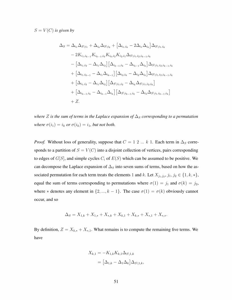
𝑆 = 𝑉 (𝐶) is given by

∆𝑆 = ∆𝑖1∆𝑆∖𝑖1 + ∆𝑖𝑘∆𝑆∖𝑖𝑘 +[∆𝑖1,𝑖𝑘 − 2∆𝑖1∆𝑖𝑘

]∆𝑆∖𝑖1,𝑖𝑘

− 2𝐾𝑖1,𝑖𝑘−1𝐾𝑖𝑘−1,𝑖𝑘𝐾𝑖𝑘,𝑖2𝐾𝑖2,𝑖1∆𝑆∖𝑖1,𝑖2,𝑖𝑘−1,𝑖𝑘

−[∆𝑖1,𝑖2 −∆𝑖1∆𝑖2

][∆𝑖𝑘−1,𝑖𝑘 −∆𝑖𝑘−1

∆𝑖𝑘

]∆𝑆∖𝑖1,𝑖2,𝑖𝑘−1,𝑖𝑘

+[∆𝑖1,𝑖𝑘−1

−∆𝑖1∆𝑖𝑘−1

][∆𝑖2,𝑖𝑘 −∆𝑖2∆𝑖𝑘

]∆𝑆∖𝑖1,𝑖2,𝑖𝑘−1,𝑖𝑘

+[∆𝑖1,𝑖2 −∆𝑖1∆𝑖2

][∆𝑆∖𝑖1,𝑖2 −∆𝑖𝑘∆𝑆∖𝑖1,𝑖2,𝑖𝑘

]+[∆𝑖𝑘−1,𝑖𝑘 −∆𝑖𝑘−1

∆𝑖𝑘

][∆𝑆∖𝑖𝑘−1,𝑖𝑘 −∆𝑖2∆𝑆∖𝑖1,𝑖𝑘−1,𝑖𝑘

]+ 𝑍.

where 𝑍 is the sum of terms in the Laplace expansion of ∆𝑆 corresponding to a permutation

where 𝜎(𝑖1) = 𝑖𝑘 or 𝜎(𝑖𝑘) = 𝑖1, but not both.

Proof. Without loss of generality, suppose that 𝐶 = 1 2 ... 𝑘 1. Each term in ∆𝑆 corre-

sponds to a partition of 𝑆 = 𝑉 (𝐶) into a disjoint collection of vertices, pairs corresponding

to edges of 𝐺[𝑆], and simple cycles 𝐶𝑖 of 𝐸(𝑆) which can be assumed to be positive. We

can decompose the Laplace expansion of ∆𝑆 into seven sums of terms, based on how the as-

sociated permutation for each term treats the elements 1 and 𝑘. Let 𝑋𝑗1,𝑗2 , 𝑗1, 𝑗2 ∈ 1, 𝑘, *,

equal the sum of terms corresponding to permutations where 𝜎(1) = 𝑗1 and 𝜎(𝑘) = 𝑗2,

where * denotes any element in 2, ..., 𝑘 − 1. The case 𝜎(1) = 𝜎(𝑘) obviously cannot

occur, and so

∆𝑆 = 𝑋1,𝑘 + 𝑋1,* + 𝑋*,𝑘 + 𝑋𝑘,1 + 𝑋𝑘,* + 𝑋*,1 + 𝑋*,*.

By definition, 𝑍 = 𝑋𝑘,* + 𝑋*,1. What remains is to compute the remaining five terms. We

have

𝑋𝑘,1 = −𝐾1,𝑘𝐾𝑘,1∆𝑆∖1,𝑘

=[∆1,𝑘 −∆1∆𝑘

]∆𝑆∖1,𝑘,

51

𝑋1,𝑘 = ∆1∆𝑘∆𝑆∖1,𝑘,

𝑋1,𝑘 + 𝑋1,* = ∆1∆𝑆∖1,

𝑋1,𝑘 + 𝑋*,𝑘 = ∆𝑘∆𝑆∖𝑘,

and so

∆𝑆 = ∆1∆𝑆∖1 + ∆𝑘∆𝑆∖𝑘 +[∆1,𝑘 − 2∆1∆𝑘

]∆𝑆∖1,𝑘 + 𝑋*,* + 𝑍.

The sum 𝑋*,* corresponds to permutations where 𝜎(1) /∈ 1, 𝑘 and 𝜎(𝑘) /∈ 1, 𝑘.

We first show that the only permutations that satisfy these two properties take the form

𝜎2(1) = 1 or 𝜎2(𝑘) = 𝑘 (or both), or contain both 1 and 𝑘 in the same cycle. Suppose to

the contrary, that there exists some permutation where 1 and 𝑘 are not in the same cycle,

and both are in cycles of length at least three. Then in 𝐺[𝑆] both vertices 1 and 𝑘 contain

a chord emanating from them. By Property (ii) of Lemma 6, each has exactly one chord

and these chords are 1, 𝑘 − 1 and 2, 𝑘. The cycle containing 1 must also contain 2 and

𝑘 − 1, and the cycle containing 𝑘 must also contain 2 and 𝑘 − 1, a contradiction.

In addition, we note that, also by the above analysis, the only cycles (of a permutation)

that can contain both 1 and 𝑘 without having 𝜎(1) = 𝑘 or 𝜎(𝑘) = 1 are given by (1 2 𝑘 𝑘−1)

and (1 𝑘− 1 𝑘 2). Therefore, we can decompose 𝑋*,* further into the sum of five terms. Let

• 𝑌1 = the sum of terms corresponding to permutations containing either (1 2 𝑘 𝑘 − 1)

or (1 𝑘 − 1 𝑘 2),

• 𝑌2 = the sum of terms corresponding to permutations containing (1 2) and (𝑘 − 1 𝑘),

• 𝑌3 = the sum of terms corresponding to permutations containing (1 𝑘 − 1) and (2 𝑘),

• 𝑌4 = the sum of terms corresponding to permutations containing (1 2) and where

𝜎(𝑘) = 𝑘 − 1, 𝑘,

• 𝑌5 = the sum of terms corresponding to permutations containing (𝑘− 1 𝑘) and where

𝜎(1) = 1, 2.

52

𝑌1 and 𝑌3 are only non-zero if 1, 𝑘 − 1 and 2, 𝑘 are both chords of 𝐶. 𝑌4 is only

non-zero if there is a chord incident to 𝑘, and 𝑌5 is only non-zero if there is a chord incident

to 1. We have 𝑋*,* = 𝑌1 + 𝑌2 + 𝑌3 + 𝑌4 + 𝑌5, and

𝑌1 = −2𝐾1,𝑘−1𝐾𝑘−1,𝑘𝐾𝑘,2𝐾2,1∆𝑆∖1,2,𝑘−1,𝑘,

𝑌2 = 𝐾1,2𝐾2,1𝐾𝑘−1,𝑘𝐾𝑘,𝑘−1∆𝑆∖1,2,𝑘−1,𝑘

=[∆1,2 −∆1∆2

][∆𝑘−1,𝑘 −∆𝑘−1∆𝑘

]∆𝑆∖1,2,𝑘−1,𝑘,

𝑌3 = 𝐾1,𝑘−1𝐾𝑘−1,1𝐾2,𝑘𝐾𝑘,2∆𝑆∖1,2,𝑘−1,𝑘

=[∆1,𝑘−1 −∆1∆𝑘−1

][∆2,𝑘 −∆2∆𝑘

]∆𝑆∖1,2,𝑘−1,𝑘,

𝑌2 + 𝑌4 = −𝐾1,2𝐾2,1

[∆𝑆∖1,2 −∆𝑘∆𝑆∖1,2,𝑘

]=[∆1,2 −∆1∆2

][∆𝑆∖1,2 −∆𝑘∆𝑆∖1,2,𝑘

],

𝑌2 + 𝑌5 = −𝐾𝑘−1,𝑘𝐾𝑘,𝑘−1

[∆𝑆∖𝑘−1,𝑘 −∆1∆𝑆∖1,𝑘−1,𝑘

]=[∆𝑘−1,𝑘 −∆𝑘−1∆𝑘

][∆𝑆∖𝑘−1,𝑘 −∆2∆𝑆∖1,𝑘−1,𝑘

].

Combining all of these terms gives us

𝑋*,* = −2𝐾1,𝑘−1𝐾𝑘−1,𝑘𝐾𝑘,2𝐾2,1∆𝑆∖1,2,𝑘−1,𝑘

−[∆1,2 −∆1∆2

][∆𝑘−1,𝑘 −∆𝑘−1∆𝑘

]∆𝑆∖1,2,𝑘−1,𝑘

+[∆1,𝑘−1 −∆1∆𝑘−1

][∆2,𝑘 −∆2∆𝑘

]∆𝑆∖1,2,𝑘−1,𝑘

+[∆1,2 −∆1∆2

][∆𝑆∖1,2 −∆𝑘∆𝑆∖1,2,𝑘

]+[∆𝑘−1,𝑘 −∆𝑘−1∆𝑘

][∆𝑆∖𝑘−1,𝑘 −∆2∆𝑆∖1,𝑘−1,𝑘

].

53

Combining our formula for 𝑋*,* with our formula for ∆𝑆 leads to the desired result

∆𝑆 = ∆1∆𝑆∖1 + ∆𝑘∆𝑆∖𝑘 +[∆1,𝑘 − 2∆1∆𝑘

]∆𝑆∖1,𝑘

− 2𝐾1,𝑘−1𝐾𝑘−1,𝑘𝐾𝑘,2𝐾2,1∆𝑆∖1,2,𝑘−1,𝑘

−[∆1,2 −∆1∆2

][∆𝑘−1,𝑘 −∆𝑘−1∆𝑘

]∆𝑆∖1,2,𝑘−1,𝑘

+[∆1,𝑘−1 −∆1∆𝑘−1

][∆2,𝑘 −∆2∆𝑘

]∆𝑆∖1,2,𝑘−1,𝑘

+[∆1,2 −∆1∆2

][∆𝑆∖1,2 −∆𝑘∆𝑆∖1,2,𝑘

]+[∆𝑘−1,𝑘 −∆𝑘−1∆𝑘

][∆𝑆∖𝑘−1,𝑘 −∆2∆𝑆∖1,𝑘−1,𝑘

]+ 𝑍.

Lemma 9. Let 𝐾 ∈ 𝒦 have two-connected charged sparsity graph 𝐺 = ([𝑁 ], 𝐸, 𝜖), and

𝐶 = 𝑖1 ... 𝑖𝑘 𝑖1 be a positive simple cycle of 𝐺 whose chords 𝛾(𝐶) satisfy Properties (i)-(iii)

of Lemma 6, with vertices ordered as in Lemma 7. Let 𝑍 equal the sum of terms in the

Laplace expansion of ∆𝑆 , 𝑆 = 𝑉 (𝐶), corresponding to a permutation where 𝜎(𝑖1) = 𝑖𝑘

or 𝜎(𝑖𝑘) = 𝑖1, but not both. Let 𝑈 ⊂ 𝑆2 be the set of pairs (𝑎, 𝑏), 𝑎 < 𝑏, for which

𝑖𝑎, 𝑖𝑏−1, 𝑖𝑎+1, 𝑖𝑏 ∈ 𝛾(𝐶), i.e., cycle edges 𝑖𝑎, 𝑖𝑎+1 and 𝑖𝑏−1, 𝑖𝑏) have a pair of

crossed chords between them. Then 𝑍 is equal to

2 (−1)𝑘+1𝐾𝑖𝑘,𝑖1

𝑘−1∏𝑗=1

𝐾𝑖𝑗 ,𝑖𝑗+1

∏(𝑎,𝑏)∈𝑈

[1−

𝜖𝑖𝑎,𝑖𝑎+1𝐾𝑖𝑏−1,𝑖𝑎𝐾𝑖𝑎+1,𝑖𝑏

𝐾𝑖𝑎,𝑖𝑎+1𝐾𝑖𝑏−1,𝑖𝑏

].

Proof. Without loss of generality, suppose that 𝐺 is labelled so that 𝐶 = 1 2 ... 𝑘 1.

Edge 1, 𝑘 satisfies Property (ii) of Lemma 7, and so every positive simple cycle of 𝐺[𝑆]

containing 1, 𝑘 spans 𝑆 and contains only edges in 𝐸(𝐶) and pairs of crossing chords.

Therefore, we may assume without loss of generality that 𝐺[𝑆] contains 𝑝 pairs of crossing

chords, and no other chords. If 𝑝 = 0, then 𝐶 is an induced cycle and the result follows

immediately.

There are 2𝑝 Hamiltonian 1 − 𝑘 paths in 𝐺[𝑆] not containing 1, 𝑘, corresponding

to the 𝑝 binary choices of whether to use each pair of crossing chords or not. Let us

54

denote these paths from 1 to 𝑘 by 𝑃 1,𝑘𝜃 , where 𝜃 ∈ Z𝑝

2, and 𝜃𝑖 equals one if the 𝑖𝑡ℎ crossing

is used in the path (ordered based on increasing distance to 1, 𝑘), and zero otherwise.

In particular, 𝑃 1,𝑘0 corresponds to the path = 1 2 ... 𝑘. We only consider paths with

the orientation 1 → 𝑘, as all cycles under consideration are positive, and the opposite

orientation has the same sum. Denoting the product of the terms of 𝐾 corresponding to the

path 𝑃 1,𝑘𝜃 = 1 = ℓ1 ℓ2 ... ℓ𝑘 = 𝑘, by

𝐾(𝑃 1,𝑘𝜃

)=

𝑘−1∏𝑗=1

𝐾ℓ𝑗 ,ℓ𝑗+1,

we have

𝑍 = 2 (−1)𝑘+1𝐾𝑘,1𝐾(𝑃 1,𝑘0

)∑𝜃∈Z𝑝

2

𝐾(𝑃 1,𝑘𝜃

)𝐾(𝑃 1,𝑘0

) ,where

𝐾(𝑃 1,𝑘0

)=

𝑘−1∏𝑗=1

𝐾𝑗,𝑗+1.

Suppose that the first possible crossing occurs at cycle edges 𝑎, 𝑎 + 1 and 𝑏 − 1, 𝑏,

𝑎 < 𝑏, i.e., 𝑎, 𝑏− 1 and 𝑎 + 1, 𝑏 are crossing chords. Then

𝑍 = 2 (−1)𝑘+1 𝐾𝑘,1

𝑘−1∏𝑗=1

𝐾𝑗,𝑗+1

∑𝜃∈Z𝑝

2

𝐾(𝑃 𝑎,𝑏𝜃

)𝐾(𝑃 𝑎,𝑏0

) .We have ∑

𝜃∈Z𝑝2

𝐾(𝑃 𝑎,𝑏𝜃

)=∑𝜃1=0

𝐾(𝑃 𝑎,𝑏𝜃

)+∑𝜃1=1

𝐾(𝑃 𝑎,𝑏𝜃

),

and

∑𝜃1=0

𝐾(𝑃 𝑎,𝑏𝜃

)= 𝐾𝑎,𝑎+1𝐾𝑏−1,𝑏

∑𝜃′∈Z𝑝−1

2

𝐾(𝑃 𝑎+1,𝑏−1𝜃′

),

55

∑𝜃1=1

𝐾(𝑃 𝑎,𝑏𝜃

)= 𝐾𝑎,𝑏−1𝐾𝑎+1,𝑏

∑𝜃′∈Z𝑝−1

2

𝐾(𝑃 𝑏−1,𝑎+1𝜃′

)= 𝐾𝑎,𝑏−1𝐾𝑎+1,𝑏

∑𝜃′∈Z𝑝−1

2

𝐾(𝑃 𝑎+1,𝑏−1𝜃′

)𝜖(𝑃 𝑎+1,𝑏−1𝜃′

).

By Property (i) of Lemma 6, 𝜖(𝐶(𝑎, 𝑏− 1)

)= −1, and so

𝜖(𝑃 𝑎+1,𝑏−1𝜃′

)= −𝜖𝑏−1,𝑎𝜖𝑎,𝑎+1 and 𝐾𝑎,𝑏−1𝜖

(𝑃 𝑎+1,𝑏−1𝜃′

)= −𝜖𝑎,𝑎+1𝐾𝑏−1,𝑎.

This implies that

∑𝜃∈Z𝑝

2

𝐾(𝑃 𝑎,𝑏𝜃

)=(𝐾𝑎,𝑎+1𝐾𝑏−1,𝑏 − 𝜖𝑎,𝑎+1𝐾𝑏−1,𝑎𝐾𝑎+1,𝑏

) ∑𝜃′∈Z𝑝−1

2

𝐾(𝑃 𝑎+1,𝑏−1𝜃′

),

and that

∑𝜃∈Z𝑝

2

𝐾(𝑃 𝑎,𝑏𝜃

)𝐾(𝑃 𝑎,𝑏0

) =

(1− 𝜖𝑎,𝑎+1𝐾𝑏−1,𝑎𝐾𝑎+1,𝑏

𝐾𝑎,𝑎+1𝐾𝑏−1,𝑏

) ∑𝜃′∈Z𝑝−1

2

𝐾(𝑃 𝑎+1,𝑏−1𝜃′

)𝐾(𝑃 𝑎+1,𝑏−10

) .Repeating the above procedure for the remaining 𝑝− 1 crossings completes the proof.

Equipped with Lemmas 6, 7, 8, and 9, we can now make a key observation. Suppose that

we have a simple cycle basis 𝑥1, ..., 𝑥𝜈−1 for 𝒞+(𝐺) whose corresponding cycles all satisfy

Properties (i)-(iii) of Lemma 6. Of course, a minimal simple cycle basis satisfies this, but in

Subsections 2.3.2 and 2.3.3 we will consider alternate bases that also satisfy these conditions

and may be easier to compute in practice. For cycles 𝐶 of length at most four, we have

already detailed how to compute 𝑠(𝐶), and this computation requires only principal minors

corresponding to subsets of 𝑉 (𝐶). When 𝐶 is of length greater than four, by Lemmas 8

and 9, we can also compute 𝑠(𝐶), using only principal minors corresponding to subsets

of 𝑉 (𝐶), as the quantity sgn(𝐾𝑖1,𝑖𝑘−1𝐾𝑖𝑘−1,𝑖𝑘𝐾𝑖𝑘,𝑖2𝐾𝑖2,𝑖1) in Lemma 8 corresponds to a

positive four-cycle, and in Lemma 9 the quantity

sgn(

1−𝜖𝑖𝑎,𝑖𝑎+1𝐾𝑖𝑏−1,𝑖𝑎𝐾𝑖𝑎+1,𝑖𝑏

𝐾𝑖𝑎,𝑖𝑎+1𝐾𝑖𝑏−1,𝑖𝑏

)

56

equals +1 if |𝐾𝑖𝑎,𝑖𝑎+1𝐾𝑖𝑏−1,𝑖𝑏| > |𝐾𝑖𝑏−1,𝑖𝑎𝐾𝑖𝑎+1,𝑖𝑏| and equals

−𝜖𝑖𝑎,𝑖𝑎+1𝜖𝑖𝑏−1,𝑖𝑏 sgn(𝐾𝑖𝑎,𝑖𝑎+1𝐾𝑖𝑎+1,𝑖𝑏𝐾𝑖𝑏,𝑖𝑏−1

𝐾𝑖𝑏−1,𝑖𝑎

)if |𝐾𝑖𝑎,𝑖𝑎+1𝐾𝑖𝑏−1,𝑖𝑏| < |𝐾𝑖𝑏−1,𝑖𝑎𝐾𝑖𝑎+1,𝑖𝑏|. By Condition (2.6), we have |𝐾𝑖𝑎,𝑖𝑎+1𝐾𝑖𝑏−1,𝑖𝑏| =

|𝐾𝑖𝑏−1,𝑖𝑎𝐾𝑖𝑎+1,𝑖𝑏|. Therefore, given a simple cycle basis 𝑥1, ..., 𝑥𝜈−1 whose corresponding

cycles satisfy Properties (i)-(iii) of Lemma 6, we can compute 𝑠(𝐶) for every such cycle

in the basis using only principal minors of size at most the length of the longest cycle in

the basis. Given this fact, we are now prepared to answer Question (2.7) and provide an

alternate proof for Question (2.8) through the following proposition and theorem.

Proposition 4. Let 𝐾 ∈ 𝒦, with charged sparsity graph 𝐺 = ([𝑁 ], 𝐸, 𝜖). The set of 𝐾 ′ ∈ 𝒦

that satisfy ∆𝑆(𝐾) = ∆𝑆(𝐾 ′) for all 𝑆 ⊂ [𝑁 ] is exactly the set generated by 𝐾 and the

operations

𝒟𝑁 -similarity: 𝐾 → 𝐷𝐾𝐷, where 𝐷 ∈ R𝑁×𝑁 is an arbitrary involutory diagonal

matrix, i.e., 𝐷 has entries ±1 on the diagonal, and

block transpose: 𝐾 → 𝐾 ′, where 𝐾 ′𝑖,𝑗 = 𝐾𝑗,𝑖 for all 𝑖, 𝑗 ∈ 𝑉 (𝐻) for some block 𝐻 , and

𝐾 ′𝑖,𝑗 = 𝐾𝑖,𝑗 otherwise.

Proof. We first verify that the 𝒟𝑁 -similarity and block transpose operations both preserve

principal minors. The determinant is multiplicative, and so principal minors are immediately

preserved under 𝒟𝑁 -similarity, as the principal submatrix of 𝐷𝐾𝐷 corresponding to 𝑆 is

equal to the product of the principal submatrices corresponding to 𝑆 of the three matrices 𝐷,

𝐾, 𝐷, and so

∆𝑆(𝐷𝐾𝐷) = ∆𝑆(𝐷)∆𝑆(𝐾)∆𝑆(𝐷) = ∆𝑆(𝐾).

For the block transpose operation, we note that the transpose leaves the determinant un-

changed. By equation (2.10), the principal minors of a matrix are uniquely determined by the

principal minors of the matrices corresponding to the blocks of 𝐺. As the transpose of any

block also leaves the principal minors corresponding to subsets of other blocks unchanged,

principal minors are preserved under 𝒟𝑁 -similarity.

57

What remains is to show that if 𝐾 ′ satisfies ∆𝑆(𝐾) = ∆𝑆(𝐾 ′) for all 𝑆 ⊂ [𝑁 ], then 𝐾 ′

is generated by 𝐾 and the above two operations. Without loss of generality, we may suppose

that the shared charged sparsity graph 𝐺 = ([𝑁 ], 𝐸, 𝜖) of 𝐾 and 𝐾 ′ is two-connected, as the

general case follows from this one. We will transform 𝐾 ′ to 𝐾 by first making them agree

for entries corresponding to a spanning tree and a negative edge of 𝐺, and then observing

that by Lemmas 8 and 9, this property implies that all entries agree.

Let 𝐶 ′ be an arbitrary negative simple cycle of 𝐺, 𝑒 ∈ 𝐸(𝐶 ′) be a negative edge in 𝐶 ′,

and 𝑇 be a spanning tree of 𝐺 containing the edges 𝐸(𝐶 ′) ∖ 𝑒. By applying 𝒟𝑁 -similarity

and block transpose to 𝐾 ′, we can produce a matrix that agrees with 𝐾 for all entries

corresponding to edges in 𝐸(𝑇 ) ∪ 𝑒. We perform this procedure in three steps, first by

making 𝐾 ′ agree with 𝐾 for edges in 𝐸(𝑇 ), then for edge 𝑒, and then finally fixing any

edges in 𝐸(𝑇 ) for which the matrices no longer agree.

First, we make 𝐾 ′ and 𝐾 agree for edges in 𝐸(𝑇 ). Suppose that 𝐾 ′𝑝,𝑞 = −𝐾𝑝,𝑞 for some

𝑝, 𝑞 ∈ 𝐸(𝑇 ). Let 𝑈 ⊂ [𝑁 ] be the set of vertices connected to 𝑝 in the forest 𝑇 ∖ 𝑝, 𝑞

(the removal of edge 𝑝, 𝑞 from 𝑇 ), and be the diagonal matrix with 𝑖,𝑖 = +1 if 𝑖 ∈ 𝑈

and 𝑖,𝑖 = −1 if 𝑖 ∈ 𝑈 . The matrix 𝐾 ′ satisfies

[𝐾 ′

]𝑝,𝑞

= 𝑝,𝑝𝐾′𝑝,𝑞𝑞,𝑞 = −𝐾 ′

𝑝,𝑞 = 𝐾𝑝,𝑞,

and[𝐾 ′

]𝑖,𝑗

= 𝐾 ′𝑖,𝑗 for any 𝑖, 𝑗 either both in 𝑈 or neither in 𝑈 (and therefore for all

edges 𝑖, 𝑗 ∈ 𝐸(𝑇 ) ∖ 𝑝, 𝑞). Repeating this procedure for every edge 𝑝, 𝑞 ∈ 𝐸(𝑇 ) for

which 𝐾 ′𝑝,𝑞 = −𝐾𝑝,𝑞 results in a matrix that agrees with 𝐾 for all entries corresponding to

edges in 𝐸(𝑇 ).

Next, we make our matrix and 𝐾 agree for the edge 𝑒. If our matrix already agrees for

edge 𝑒, then we are done with this part of the proof, and we denote the resulting matrix by

. If our resulting matrix does not agree, then, by taking the transpose of this matrix, we

have a new matrix that now agrees with 𝐾 for all edges 𝐸(𝑇 )∪ 𝑒, except for negative edges

in 𝐸(𝑇 ). By repeating the 𝒟𝑁 -similarity operation again on negative edges of 𝐸(𝑇 ), we

again obtain a matrix that agrees with 𝐾 on the edges of 𝐸(𝑇 ), but now also agrees on the

58

edge 𝑒, as there is an even number of negative edges in the path between the vertices of 𝑒 in

the tree 𝑇 . We now have a matrix that agrees with 𝐾 for all entries corresponding to edges

in 𝐸(𝑇 ) ∪ 𝑒, and we denote this matrix by .

Finally, we aim to show that agreement on the edges 𝐸(𝑇 ) ∪ 𝑒 already implies that

= 𝐾. Let 𝑖, 𝑗 be an arbitrary edge not in 𝐸(𝑇 ) ∪ 𝑒, and 𝐶 be the simple cycle

containing edge 𝑖, 𝑗 and the unique 𝑖− 𝑗 path in the tree 𝑇 . By Lemmas 8 and 9, the value

of 𝑠𝐾(𝐶) can be computed for every cycle corresponding to an incidence vector in a minimal

simple cycle basis of 𝒞+(𝐺) using only principal minors. Then 𝑠𝐾(𝐶) can be computed

using principal minors and 𝑠𝐾(𝐶 ′), as the incidence vector for 𝐶 ′ combined with a minimal

positive simple cycle basis forms a basis for 𝒞(𝐺). By assumption, ∆𝑆(𝐾) = ∆𝑆() for

all 𝑆 ⊂ [𝑁 ], and, by construction, 𝑠𝐾(𝐶 ′) = 𝑠(𝐶 ′). Therefore, 𝑠𝐾(𝐶) = 𝑠(𝐶) for all

𝑖, 𝑗 not in 𝐸(𝑇 ) ∪ 𝑒, and so = 𝐾.

Theorem 5. Let 𝐾 ∈ 𝒦, with charged sparsity graph 𝐺 = ([𝑁 ], 𝐸, 𝜖). Let ℓ+ ≥ 3 be the

simple cycle sparsity of 𝒞+(𝐺). Then any matrix 𝐾 ′ ∈ 𝒦 with ∆𝑆(𝐾) = ∆𝑆(𝐾 ′) for all

|𝑆| ≤ ℓ+ also satisfies ∆𝑆(𝐾) = ∆𝑆(𝐾 ′) for all 𝑆 ⊂ [𝑁 ], and there exists a matrix ∈ 𝒦

with ∆𝑆() = ∆𝑆(𝐾) for all |𝑆| < ℓ+ but ∆𝑆() = ∆𝑆(𝐾) for some 𝑆.

Proof. The first part of theorem follows almost immediately from Lemmas 8 and 9. It

suffices to consider a matrix 𝐾 ∈ 𝒦 with a two-connected charged sparsity graph 𝐺 =

([𝑁 ], 𝐸, 𝜖), as the more general case follows from this one. By Lemmas 8, and 9, the

quantity 𝑠(𝐶) is computable for all simple cycles 𝐶 in a minimal cycle basis for 𝒞+(𝐺)

(and therefore for all positive simple cycles), using only principal minors of size at most

the length of the longest cycle in the basis, which in this case is the simple cycle sparsity

ℓ+ of 𝒞+(𝐺). The values 𝑠(𝐶) for positive simple cycles combined with the magnitude of

the entries of 𝐾 and the charge function 𝜖 uniquely determines all principal minors, as each

term in the Laplace expansion of some ∆𝑆(𝐾) corresponds to a partitioning of 𝑆 into a

disjoint collection of vertices, pairs corresponding to edges, and oriented versions of positive

simple cycles of 𝐸(𝑆). This completes the first portion of the proof.

Next, we explicitly construct a matrix that agrees with 𝐾 in the first ℓ+ − 1 principal

minors (ℓ+ ≥ 3), but disagrees on a principal minor of order ℓ+. To do so, we consider a

59

minimal simple cycle basis𝜒𝐶1 , ..., 𝜒𝐶𝜈−1

of 𝒞+(𝐺), ordered so that |𝐶1| ≥ |𝐶2| ≥ ... ≥

|𝐶𝜈−1|. By definition, ℓ+ = |𝐶1|. Let be a matrix satisfying

𝑖,𝑖 = 𝐾𝑖,𝑖 for 𝑖 ∈ [𝑁 ], 𝑖,𝑗𝑗,𝑖 = 𝐾𝑖,𝑗𝐾𝑗,𝑖 for 𝑖, 𝑗 ∈ [𝑁 ],

and

𝑠(𝐶𝑖) =

⎧⎪⎨⎪⎩ 𝑠𝐾(𝐶𝑖) if 𝑖 > 1

−𝑠𝐾(𝐶𝑖) if 𝑖 = 1

.

The matrix and 𝐾 agree on all principal minors of order at most ℓ+ − 1, for if there was

a principal minor where they disagreed, this would imply that there is a positive simple

cycle of length less than ℓ+ whose incidence vector is not in the span of 𝜒𝐶2 , ..., 𝜒𝐶𝜈−1, a

contradiction. To complete the proof, it suffices to show that ∆𝑉 (𝐶1)() = ∆𝑉 (𝐶1)(𝐾).

To do so, we consider three different cases, depending on the length of 𝐶1. If 𝐶1 is

a three-cycle, then 𝐶1 is an induced cycle and the result follows immediately. If 𝐶1 is a

four-cycle, 𝐺[𝑉 (𝐶1)] may possibly have multiple positive four-cycles. However, in this

case the quantity 𝑍 from Equation (2.11) is distinct for and 𝐾, as 𝐾 ∈ 𝒦. Finally,

we consider the general case when |𝐶1| > 4. By Lemma 8, all terms of ∆𝑉 (𝐶)(𝐾) (and

∆𝑉 (𝐶)()) except for 𝑍 depend only on principal minors of order at most ℓ+ − 1. We

denote the quantity 𝑍 from Lemma 8 for 𝐾 and by 𝑍 and 𝑍 respectively. By Lemma 9,

the magnitude of 𝑍 and 𝑍 depend only on principal minors of order at most four, and so

|𝑍| = |𝑍|. In addition, because 𝐾 ∈ 𝒦, 𝑍 = 0. The quantities 𝑍 and 𝑍 are equal in sign if

and only if 𝑠(𝐶1) = 𝑠𝐾(𝐶1), and therefore ∆𝑉 (𝐶1)() = ∆𝑉 (𝐶1)(𝐾).

2.3.2 Efficiently Recovering a Matrix from its Principal Minors

In Subsection 2.3.1, we characterized both the set of magnitude-symmetric matrices in 𝒦

that share a given set of principal minors, and noted that principal minors of order ≤ ℓ+

uniquely determine principal minors of all orders, where ℓ+ is the simple cycle sparsity of

𝒞+(𝐺) and is computable using principal minors of order one and two. In this subsection,

we make use of a number of theoretical results of Subsection 2.3.1 to formally describe a

60

polynomial time algorithm to produce a magnitude-symmetric matrix 𝐾 with prescribed

principal minors. We provide a high-level description and discussion of this algorithm below,

and save the description of a key subroutine for computing a positive simple cycle basis for

after the overall description and proof.

An Efficient Algorithm

Our formal algorithm proceeds by completing a number of high-level tasks, which we

describe below. This procedure is very similar in nature to the algorithm implicitly described

and used in the proofs of Proposition 4 and Theorem 5. The main difference between the

algorithmic procedure alluded to in Subsection 2.3.1 and this algorithm is the computation

of a positive simple cycle basis. Unlike 𝒞(𝐺), there is no known polynomial time algorithm

to compute a minimal simple cycle basis for 𝒞+(𝐺), and a decision version of this problem

may indeed be NP-hard. Our algorithm, which we denote by RECOVERK(∆𝑆𝑆⊂[𝑁 ]

),

proceeds in five main steps:

Step 1: Compute |𝐾𝑖,𝑗|, 𝑖, 𝑗 ∈ [𝑁 ], and the charged sparsity graph 𝐺 = ([𝑁 ], 𝐸, 𝜖).

We recall that 𝐾𝑖,𝑖 = ∆𝑖 and |𝐾𝑖,𝑗| = |𝐾𝑗,𝑖| =√|∆𝑖∆𝑗 −∆𝑖,𝑗|. The edges 𝑖, 𝑗 ∈

𝐸(𝐺) correspond to non-zero off-diagonal entries |𝐾𝑖,𝑗| = 0, and the function 𝜖 is given

by 𝜖𝑖,𝑗 = sgn(∆𝑖∆𝑗 −∆𝑖,𝑗).

Step 2: For every block 𝐻 of 𝐺, compute a simple cycle basis 𝑥1, ..., 𝑥𝑘 of 𝒞+(𝐻).

In the proof of Proposition 3, we defined an efficient algorithm to compute a simple

cycle basis of 𝒞+(𝐻) for any two-connected graph 𝐻 . This algorithm makes use of the

property that every two-connected graph has an open ear decomposition. Unfortunately,

this algorithm has no provable guarantees on the length of the longest cycle in the basis.

For this reason, we introduce an alternate efficient algorithm below that computes a

simple cycle basis of 𝒞+(𝐻) consisting of cycles all of length at most 3𝜑𝐻 , where 𝜑𝐻 is

61

the maximum length of a shortest cycle between any two edges in 𝐻 , i.e.,

𝜑𝐻 := max𝑒,𝑒′∈𝐸(𝐻)

minsimple cycle 𝐶𝑠.𝑡. 𝑒,𝑒′∈𝐸(𝐶)

|𝐶|

with 𝜑𝐻 := 2 if 𝐻 is acyclic. The existence of a simple cycle through any two edges

of a 2-connected graph can be deduced from the existence of two vertex-disjoint paths

between newly added midpoints of these two edges. The resulting simple cycle basis

also maximizes the number of three- and four-cycles it contains. This is a key property

which allows us to limit the number of principal minors that we query.

Step 3: For every block 𝐻 of 𝐺, convert 𝑥1, ..., 𝑥𝑘 into a simple cycle basis satisfying

Properties (i)-(iii) of Lemma 6.

If there was an efficient algorithm for computing a minimal simple cycle basis for

𝒞+(𝐻), by Lemma 6, we would be done (and there would be no need for the previous

step). However, there is currently no known algorithm for this, and a decision version of

this problem may be NP-hard. By using the simple cycle basis from Step 2 and iteratively

removing chords, we can create a basis that satisfies the same three key properties (in

Lemma 6) that a minimal simple cycle basis does. In addition, the lengths of the cycles

in this basis are no larger than those of Step 2, i.e., no procedure in Step 3 ever increases

the length of a cycle.

The procedure for this is quite intuitive. Given a cycle 𝐶 in the basis, we efficiently

check that 𝛾(𝐶) satisfies Properties (i)-(iii) of Lemma 6. If all properties hold, we are

done, and check another cycle in the basis, until all cycles satisfy the desired properties.

In each case, if a given property does not hold, then, by the proof of Lemma 6, we can

efficiently compute an alternate cycle 𝐶 ′, |𝐶 ′| < |𝐶|, that can replace 𝐶 in the simple

cycle basis for 𝒞+(𝐻), decreasing the sum of cycle lengths in the basis by at least one.

Because of this, the described procedure is a polynomial time algorithm.

62

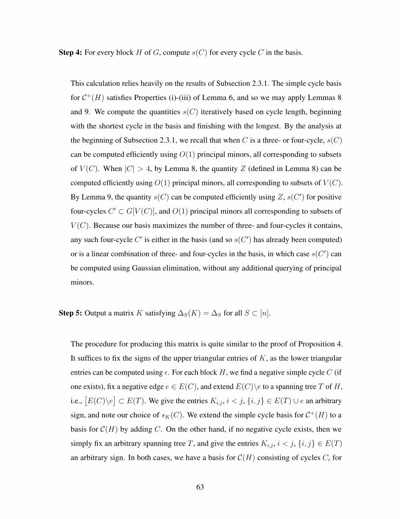
Step 4: For every block 𝐻 of 𝐺, compute 𝑠(𝐶) for every cycle 𝐶 in the basis.

This calculation relies heavily on the results of Subsection 2.3.1. The simple cycle basis

for 𝒞+(𝐻) satisfies Properties (i)-(iii) of Lemma 6, and so we may apply Lemmas 8

and 9. We compute the quantities 𝑠(𝐶) iteratively based on cycle length, beginning

with the shortest cycle in the basis and finishing with the longest. By the analysis at

the beginning of Subsection 2.3.1, we recall that when 𝐶 is a three- or four-cycle, 𝑠(𝐶)

can be computed efficiently using 𝑂(1) principal minors, all corresponding to subsets

of 𝑉 (𝐶). When |𝐶| > 4, by Lemma 8, the quantity 𝑍 (defined in Lemma 8) can be

computed efficiently using 𝑂(1) principal minors, all corresponding to subsets of 𝑉 (𝐶).

By Lemma 9, the quantity 𝑠(𝐶) can be computed efficiently using 𝑍, 𝑠(𝐶 ′) for positive

four-cycles 𝐶 ′ ⊂ 𝐺[𝑉 (𝐶)], and 𝑂(1) principal minors all corresponding to subsets of

𝑉 (𝐶). Because our basis maximizes the number of three- and four-cycles it contains,

any such four-cycle 𝐶 ′ is either in the basis (and so 𝑠(𝐶 ′) has already been computed)

or is a linear combination of three- and four-cycles in the basis, in which case 𝑠(𝐶 ′) can

be computed using Gaussian elimination, without any additional querying of principal

minors.

Step 5: Output a matrix 𝐾 satisfying ∆𝑆(𝐾) = ∆𝑆 for all 𝑆 ⊂ [𝑛].

The procedure for producing this matrix is quite similar to the proof of Proposition 4.

It suffices to fix the signs of the upper triangular entries of 𝐾, as the lower triangular

entries can be computed using 𝜖. For each block 𝐻 , we find a negative simple cycle 𝐶 (if

one exists), fix a negative edge 𝑒 ∈ 𝐸(𝐶), and extend 𝐸(𝐶)∖𝑒 to a spanning tree 𝑇 of 𝐻 ,

i.e.,[𝐸(𝐶)∖𝑒

]⊂ 𝐸(𝑇 ). We give the entries 𝐾𝑖,𝑗 , 𝑖 < 𝑗, 𝑖, 𝑗 ∈ 𝐸(𝑇 ) ∪ 𝑒 an arbitrary

sign, and note our choice of 𝑠𝐾(𝐶). We extend the simple cycle basis for 𝒞+(𝐻) to a

basis for 𝒞(𝐻) by adding 𝐶. On the other hand, if no negative cycle exists, then we

simply fix an arbitrary spanning tree 𝑇 , and give the entries 𝐾𝑖,𝑗 , 𝑖 < 𝑗, 𝑖, 𝑗 ∈ 𝐸(𝑇 )

an arbitrary sign. In both cases, we have a basis for 𝒞(𝐻) consisting of cycles 𝐶𝑖 for

63

which we have computed 𝑠(𝐶𝑖). For each edge 𝑖, 𝑗 ∈ 𝐸(𝐻) corresponding to an entry

𝐾𝑖,𝑗 for which we have not fixed the sign of, we consider the cycle 𝐶 ′ consisting of the

edge 𝑖, 𝑗 and the unique 𝑖− 𝑗 path in 𝑇 . Using Gaussian elimination, we can write 𝐶 ′

as a sum of a subset of the cycles in our basis. As noted in Subsection 2.3.1, the quantity

𝑠(𝐶 ′) is simply the product of the quantities 𝑠(𝐶𝑖) for cycles 𝐶𝑖 in this sum.

A few comments are in order. Conditional on the analysis of Step 2, the above algorithm

runs in time polynomial in 𝑁 . Of course, the set ∆𝑆𝑆⊂[𝑁 ] is not polynomial in 𝑁 , but

rather than take the entire set as input, we assume the existence of some querying operation,

in which the value of any principal minor can be queried in polynomial time. Combining the

analysis of each step, we can give the following guarantee for the RECOVERK(∆𝑆𝑆⊂[𝑁 ]

)algorithm.

Theorem 6. Let ∆𝑆𝑆⊂[𝑁 ] be the principal minors of some matrix in 𝒦. The algorithm

RECOVERK(∆𝑆𝑆⊂[𝑁 ]

)computes a matrix 𝐾 ∈ 𝒦 satisfying ∆𝑆(𝐾) = ∆𝑆 for all

𝑆 ⊂ [𝑁 ]. This algorithm runs in time polynomial in 𝑁 , and queries at most 𝑂(𝑁2)

principal minors, all of order at most 3𝜑𝐺, where 𝐺 is the sparsity graph of ∆𝑆|𝑆|≤2 and

𝜑𝐺 is the maximum of 𝜑𝐻 over all blocks 𝐻 of 𝐺. In addition, there exists a matrix 𝐾 ′ ∈ 𝒦,

|𝐾 ′𝑖,𝑗| = |𝐾𝑖,𝑗|, 𝑖, 𝑗 ∈ [𝑁 ], such that any algorithm that computes a matrix with principal

minors ∆𝑆(𝐾 ′)𝑆⊂[𝑁 ] must query a principal minor of order at least 𝜑𝐺.

Proof. Conditional on the existence of the algorithm described in Step 2, i.e., an efficient

algorithm to compute a simple cycle basis for 𝒞+(𝐻) consisting of cycles of length at most

3𝜑𝐻 that maximizes the number of three- and four-cycles it contains, by the above analysis

we already have shown that the RECOVERK(∆𝑆𝑆⊂[𝑁 ]

)algorithm runs in time polynomial

in 𝑛 and queries at most 𝑂(𝑁2) principal minors.

To construct 𝐾 ′, we first consider the uncharged sparsity graph 𝐺 = ([𝑁 ], 𝐸) of 𝐾, and

let 𝑒, 𝑒′ ∈ 𝐸(𝐺) be a pair of edges for which the quantity 𝜑𝐺 is achieved (if 𝜑𝐺 = 2, we

are done). We aim to define an alternate charge function for 𝐺, show that the simple cycle

sparsity of 𝒞+(𝐺) is at least 𝜑𝐺, find a matrix 𝐾 ′ that has this charged sparsity graph, and

64

then make use of Theorem 5. Consider the charge function 𝜖 satisfying 𝜖(𝑒) = 𝜖(𝑒′) = −1,

and equal to +1 otherwise. Any simple cycle basis for the block containing 𝑒, 𝑒′ must have

a simple cycle containing both edges 𝑒, 𝑒′. By definition, the length of this cycle is at least

𝜑𝐺, and so the simple cycle sparsity of 𝒞+(𝐺) is at least 𝜑𝐺. Next, let 𝐾 ′ be an arbitrary

matrix with |𝐾 ′𝑖,𝑗| = |𝐾𝑖,𝑗|, 𝑖, 𝑗 ∈ [𝑁 ], and charged sparsity graph 𝐺 = ([𝑁 ], 𝐸, 𝜖), with 𝜖

as defined above. 𝐾 ∈ 𝒦, and so 𝐾 ′ ∈ 𝒦, and therefore, by Theorem 5, any algorithm that

computes a matrix with principal minors ∆𝑆(𝐾 ′)𝑆⊂[𝑁 ] must query a principal minor of

order at least ℓ+ ≥ 𝜑𝐺.

Computing a Simple Cycle Basis with Provable Guarantees

Next, we describe an efficient algorithm to compute a simple cycle basis for 𝒞+(𝐻)

consisting of cycles of length at most 3𝜑𝐻 . Suppose we have a two-connected graph

𝐻 = ([𝑁 ], 𝐸, 𝜖). We first compute a minimal cycle basis 𝜒𝐶1 , ..., 𝜒𝐶𝜈 of 𝒞(𝐻), where

each 𝐶𝑖 is an induced simple cycle (as argued previously, any lexicographically minimal

basis for 𝒞(𝐻) consists only of induced simple cycles). Without loss of generality, sup-

pose that 𝐶1 is the shortest negative cycle in the basis (if no negative cycle exists, we are

done). The set of incidence vectors 𝜒𝐶1 + 𝜒𝐶𝑖, 𝜖(𝐶𝑖) = −1, combined with vectors 𝜒𝐶𝑗

,

𝜖(𝐶𝑗) = +1, forms a basis for 𝒞+(𝐻), which we denote by ℬ. We will build a simple

cycle basis for 𝒞+(𝐻) by iteratively choosing incidence vectors of the form 𝜒𝐶1 + 𝜒𝐶𝑖,

𝜖(𝐶𝑖) = −1, replacing each with an incidence vector 𝜒 𝐶𝑖corresponding to a positive simple

cycle 𝐶𝑖, and iteratively updating ℬ.

Let 𝐶 := 𝐶1 + 𝐶𝑖 be a positive cycle in our basis ℬ. If 𝐶 is a simple cycle, we are done,

otherwise 𝐶 is the union of edge-disjoint simple cycles 𝐹1, ..., 𝐹𝑝 for some 𝑝 > 1. If one of

these simple cycles is positive and satisfies

𝜒𝐹𝑗∈ span

ℬ∖𝜒𝐶1 + 𝜒𝐶𝑖

,

we are done. Otherwise there is a negative simple cycle, without loss of generality given by

𝐹1. We can construct a set of 𝑝 − 1 positive cycles by adding 𝐹1 to each negative simple

65

cycle, and at least one of these cycles is not in spanℬ∖𝜒𝐶1 + 𝜒𝐶𝑖

. We now have a

positive cycle not in this span, given by the sum of two edge-disjoint negative simple cycles

𝐹1 and 𝐹𝑗 . These two cycles satisfy, by construction, |𝐹1| + |𝐹𝑗| ≤ |𝐶| ≤ 2ℓ, where ℓ is

the cycle sparsity of 𝒞(𝐻). If |𝑉 (𝐹1) ∩ 𝑉 (𝐹𝑗)| > 1, then 𝐹1 ∪ 𝐹𝑗 is two-connected, and we

may compute a simple cycle basis for 𝒞+(𝐹1 ∪ 𝐹𝑗) using the ear decomposition approach of

Proposition 3. At least one positive simple cycle in this basis satisfies our desired condition,

and the length of this positive simple cycle is at most |𝐸(𝐹1 ∪ 𝐹𝑗)| ≤ 2ℓ. If 𝐹1 ∪ 𝐹𝑗 is not

two-connected, then we compute a shortest cycle 𝐶 in 𝐸(𝐻) containing both an edge in

𝐸(𝐹1) and 𝐸(𝐹𝑗) (computed using Suurballe’s algorithm, see [109] for details). The graph

𝐻 ′ =(𝑉 (𝐹1) ∪ 𝑉 (𝐹𝑗) ∪ 𝑉 ( 𝐶), 𝐸(𝐹1) ∪ 𝐸(𝐹𝑗) ∪ 𝐸( 𝐶)

)is two-connected, and we can repeat the same procedure as above for 𝐻 ′, where, in this case,

the resulting cycle is of length at most |𝐸(𝐻 ′)| ≤ 2ℓ + 𝜑𝐻 . The additional guarantee for

maximizing the number of three- and four-cycles can be obtained easily by simply listing

all positive cycles of length three and four, combining them with the computed basis, and

performing a greedy algorithm. What remains is to note that ℓ ≤ 𝜑𝐻 . This follows quickly

from the observation that for any vertex 𝑢 in any simple cycle 𝐶 of a minimal cycle basis

for 𝒞(𝐻), there exists an edge 𝑣, 𝑤 ∈ 𝐸(𝐶) such that 𝐶 is the disjoint union of a shortest

𝑢− 𝑣 path, shortest 𝑢− 𝑤 path, and 𝑣, 𝑤 [51, Theorem 3].

2.3.3 An Algorithm for Principal Minors with Noise

So far, we have exclusively considered the situation in which principal minors are known (or

can be queried) exactly. In applications related to this work, this is often not the case. The

key application of a large part of this work is signed determinantal point processes, and the

algorithmic question of learning the kernel of a signed DPP from some set of samples. Here,

for the sake of readability, we focus on the non-probabilistic setting in which, given some

matrix 𝐾 with spectral radius 𝜌(𝐾) ≤ 1, each principal minor ∆𝑆 can be queried/estimated

66

up to some absolute error term 0 < 𝛿 < 1, i.e., we are given a set ∆𝑆𝑆⊂[𝑁 ], satisfying

∆𝑆 −∆𝑆

< 𝛿 for all 𝑆 ⊂ [𝑁 ],

where ∆𝑆𝑆⊂[𝑁 ] are the principal minors of some magnitude-symmetric matrix 𝐾, and

asked to compute a matrix 𝐾 ′ minimizing

𝜌(𝐾,𝐾 ′) := min s.t.

Δ𝑆()=Δ𝑆(𝐾),𝑆⊂[𝑁 ]

| −𝐾 ′|∞,

where |𝐾 −𝐾 ′|∞ = max𝑖,𝑗 |𝐾𝑖,𝑗 −𝐾 ′𝑖,𝑗|.

In this setting, we require both a separation condition for the entries of 𝐾 and a stronger

version of Condition (2.6). Let 𝒦𝑁(𝛼, 𝛽) be the set of matrices 𝐾 ∈ R𝑁×𝑁 , 𝜌(𝐾) ≤ 1,

satisfying: |𝐾𝑖,𝑗| = |𝐾𝑗,𝑖| for 𝑖, 𝑗 ∈ [𝐾], |𝐾𝑖,𝑗| > 𝛼 or |𝐾𝑖,𝑗| = 0 for all 𝑖, 𝑗 ∈ [𝑁 ], and

If 𝐾𝑖,𝑗𝐾𝑗,𝑘𝐾𝑘,ℓ𝐾ℓ,𝑖 = 0 for 𝑖, 𝑗, 𝑘, ℓ ∈ [𝑁 ] distinct, (2.12)

then|𝐾𝑖,𝑗𝐾𝑘,ℓ| − |𝐾𝑗,𝑘𝐾ℓ,𝑖|

> 𝛽, and the sum

𝜑1𝐾𝑖,𝑗𝐾𝑗,𝑘𝐾𝑘,ℓ𝐾ℓ,𝑖 + 𝜑2𝐾𝑖,𝑗𝐾𝑗,ℓ𝐾ℓ,𝑘𝐾𝑘,𝑖

+ 𝜑3𝐾𝑖,𝑘𝐾𝑘,𝑗𝐾𝑗,ℓ𝐾ℓ,𝑖

> 𝛽 ∀𝜑 ∈ −1, 13.

The algorithm RECOVERK(∆𝑆𝑆⊂[𝑁 ]

), slightly modified, performs well for this more

general problem. Here, we briefly describe a variant of the above algorithm that performs

nearly optimally on any 𝐾 ∈ 𝒦(𝛼, 𝛽), 𝛼, 𝛽 > 0, for 𝛿 sufficiently small, and quantify the

relationship between 𝛼 and 𝛽. The algorithm to compute a 𝐾 ′ sufficiently close to 𝐾, which

we denote by RECOVERNOISYK(∆𝑆𝑆⊂[𝑁 ]; 𝛿

), proceeds in three main steps:

Step 1: Define |𝐾 ′𝑖,𝑗|, 𝑖, 𝑗 ∈ [𝑁 ], and the charged sparsity graph 𝐺 = ([𝑁 ], 𝐸, 𝜖).

67

We define

𝐾 ′𝑖,𝑖 =

⎧⎪⎨⎪⎩∆𝑖 if |∆𝑖| > 𝛿

0 otherwise,

and

𝐾 ′𝑖,𝑗𝐾

′𝑗,𝑖 =

⎧⎪⎨⎪⎩∆𝑖∆𝑗 − ∆𝑖,𝑗 if |∆𝑖∆𝑗 − ∆𝑖,𝑗| > 3𝛿 + 𝛿2

0 otherwise.

The edges 𝑖, 𝑗 ∈ 𝐸(𝐺) correspond to non-zero off-diagonal entries |𝐾 ′𝑖,𝑗| = 0, and

the function 𝜖 is given by 𝜖𝑖,𝑗 = sgn(𝐾 ′𝑖,𝑗𝐾

′𝑗,𝑖).

Step 2: For every block 𝐻 of 𝐺, compute a simple cycle basis 𝑥1, ..., 𝑥𝑘 of 𝒞+(𝐻) satis-

fying Properties (i)-(iii) of Lemma 6, and define 𝑠𝐾′(𝐶) for every cycle 𝐶 in the basis.

The computation of the simple cycle basis depends only on the graph 𝐺, and so is identi-

cal to Steps 1 and 2 of the RECOVERK algorithm. The simple cycle basis for 𝒞+(𝐻)

satisfies Properties (i)-(iii) of Lemma 6, and so we can apply Lemmas 8 and 9. We

define the quantities 𝑠𝐾′(𝐶) iteratively based on cycle length, beginning with the shortest

cycle. We begin by detailing the cases of |𝐶| = 3, then |𝐶| = 4, and then finally |𝐶| > 4.

Case I: |𝐶| = 3.

Suppose that the three-cycle 𝐶 = 𝑖 𝑗 𝑘 𝑖, 𝑖 < 𝑗 < 𝑘, is in our basis. If 𝐺 was the charged

sparsity graph of 𝐾, then the equation

𝐾𝑖,𝑗𝐾𝑗,𝑘𝐾𝑘,𝑖 = ∆𝑖∆𝑗∆𝑘 −1

2

[∆𝑖∆𝑗,𝑘 + ∆𝑗∆𝑖,𝑘 + ∆𝑘∆𝑖,𝑗

]+

1

2∆𝑖,𝑗,𝑘

would hold. For this reason, we define 𝑠𝐾′(𝐶) as

𝑠𝐾′(𝐶) = 𝜖𝑖,𝑘 sgn(2∆𝑖∆𝑗∆𝑘 −

[∆𝑖∆𝑗,𝑘 + ∆𝑗∆𝑖,𝑘 + ∆𝑘∆𝑖,𝑗

]+ ∆𝑖,𝑗,𝑘

).

68

Case II: |𝐶| = 4.

Suppose that the four-cycle 𝐶 = 𝑖 𝑗 𝑘 ℓ 𝑖, with (without loss of generality) 𝑖 < 𝑗 < 𝑘 < ℓ,

is in our basis. We note that

∆𝑖,𝑗,𝑘,ℓ = ∆𝑖,𝑗∆𝑘,ℓ + ∆𝑖,𝑘∆𝑗,ℓ + ∆𝑖,ℓ∆𝑗,𝑘 + ∆𝑖∆𝑗,𝑘,ℓ + ∆𝑗∆𝑖,𝑘,ℓ + ∆𝑘∆𝑖,𝑗,ℓ

+ ∆ℓ∆𝑖,𝑗,𝑘 − 2∆𝑖∆𝑗∆𝑘,ℓ − 2∆𝑖∆𝑘∆𝑗,ℓ − 2∆𝑖∆ℓ∆𝑗,𝑘 − 2∆𝑗∆𝑘∆𝑖,ℓ

− 2∆𝑗∆ℓ∆𝑖,𝑘 − 2∆𝑘∆ℓ∆𝑖,𝑗 + 6∆𝑖∆𝑗∆𝑘∆ℓ + 𝑍,

where 𝑍 is the sum of the terms in the Laplace expansion of ∆𝑖,𝑗,𝑘,ℓ corresponding to a

four-cycle of 𝐺[𝑖, 𝑗, 𝑘, ℓ], and define the quantity 𝑍 analogously:

𝑍 = ∆𝑖,𝑗,𝑘,ℓ − ∆𝑖,𝑗∆𝑘,ℓ − ∆𝑖,𝑘∆𝑗,ℓ − ∆𝑖,ℓ∆𝑗,𝑘 − ∆𝑖∆𝑗,𝑘,ℓ − ∆𝑗∆𝑖,𝑘,ℓ

− ∆𝑘∆𝑖,𝑗,ℓ − ∆ℓ∆𝑖,𝑗,𝑘 + 2∆𝑖∆𝑗∆𝑘,ℓ + 2∆𝑖∆𝑘∆𝑗,ℓ + 2∆𝑖∆ℓ∆𝑗,𝑘

+ 2∆𝑗∆𝑘∆𝑖,ℓ + 2∆𝑗∆ℓ∆𝑖,𝑘 + 2∆𝑘∆ℓ∆𝑖,𝑗 − 6∆𝑖∆𝑗∆𝑘∆ℓ.

We consider two cases, depending on the number of positive four-cycles in 𝐺[𝑖, 𝑗, 𝑘, ℓ].

First, suppose that 𝐶 is the only positive four-cycle in 𝐺[𝑖, 𝑗, 𝑘, ℓ]. If 𝐺 was the charged

sparsity graph of 𝐾, then 𝑍 would equal−2𝐾𝑖,𝑗𝐾𝑗,𝑘𝐾𝑘,ℓ𝐾ℓ,𝑖. For this reason, we define

𝑠𝐾′(𝐶) as

𝑠𝐾′(𝐶) = 𝜖𝑖,ℓ sgn(− 𝑍

)in this case. Next, we consider the second case, in which there is more than one

positive four-cycle in 𝐺[𝑖, 𝑗, 𝑘, ℓ], which actually implies that all three four-cycles in

𝐺[𝑖, 𝑗, 𝑘, ℓ] are positive. If 𝐺 was the charged sparsity graph of 𝐾 then 𝑍 would be

69

given by

𝑍 = −2(𝐾𝑖,𝑗𝐾𝑗,𝑘𝐾𝑘,ℓ𝐾ℓ,𝑖 + 𝐾𝑖,𝑗𝐾𝑗,ℓ𝐾ℓ,𝑘𝐾𝑘,𝑖 + 𝐾𝑖,𝑘𝐾𝑘,𝑗𝐾𝑗,ℓ𝐾ℓ,𝑖

).

For this reason, we compute an assignment of values 𝜑1, 𝜑2, 𝜑3 ∈ −1,+1 that mini-

mizes (not necessarily uniquely) the quantity𝑍/2 + 𝜑1

𝑖,𝑗𝑗,𝑘𝑘,ℓℓ,𝑖

+ 𝜑2

𝑖,𝑗𝑗,ℓℓ,𝑘𝑘,𝑖

+ 𝜑3

𝑖,𝑘𝑘,𝑗𝑗,ℓℓ,𝑖

,

and define 𝑠𝐾′(𝐶) = 𝜖𝑖,ℓ 𝜑1 in this case.

Case III: |𝐶| > 4.

Suppose that the cycle 𝐶 = 𝑖1 ... 𝑖𝑘 𝑖1, 𝑘 > 4, is in our basis, with vertices ordered to

match the ordering of Lemma 8, and define 𝑆 = 𝑖1, ..., 𝑖𝑘. Based on the equation in

Lemma 8, we define 𝑍 to equal

𝑍 = ∆𝑆 − ∆𝑖1∆𝑆∖𝑖1 − ∆𝑖𝑘∆𝑆∖𝑖𝑘 −[∆𝑖1,𝑖𝑘 − 2∆𝑖1∆𝑖𝑘

]∆𝑆∖𝑖1,𝑖𝑘

+ 2𝐾 ′𝑖1,𝑖𝑘−1

𝐾 ′𝑖𝑘−1,𝑖𝑘

𝐾 ′𝑖𝑘,𝑖2

𝐾 ′𝑖2,𝑖1

∆𝑆∖𝑖1,𝑖2,𝑖𝑘−1,𝑖𝑘

+[∆𝑖1,𝑖2 − ∆𝑖1∆𝑖2

][∆𝑖𝑘−1,𝑖𝑘 − ∆𝑖𝑘−1

∆𝑖𝑘

]∆𝑆∖𝑖1,𝑖2,𝑖𝑘−1,𝑖𝑘

−[∆𝑖1,𝑖𝑘−1

− ∆𝑖1∆𝑖𝑘−1

][∆𝑖2,𝑖𝑘 − ∆𝑖2∆𝑖𝑘

]∆𝑆∖𝑖1,𝑖2,𝑖𝑘−1,𝑖𝑘

−[∆𝑖1,𝑖2 − ∆𝑖1∆𝑖2

][∆𝑆∖𝑖1,𝑖2 − ∆𝑖𝑘∆𝑆∖𝑖1,𝑖2,𝑖𝑘

]−[∆𝑖𝑘−1,𝑖𝑘 − ∆𝑖𝑘−1

∆𝑖𝑘

][∆𝑆∖𝑖𝑘−1,𝑖𝑘 − ∆𝑖2∆𝑆∖𝑖1,𝑖𝑘−1,𝑖𝑘

],

and note that the quantity

sgn(𝐾 ′𝑖1,𝑖𝑘−1

𝐾 ′𝑖𝑘−1,𝑖𝑘

𝐾 ′𝑖𝑘,𝑖2

𝐾 ′𝑖2,𝑖1

)

is, by construction, computable using the signs of three- and four-cycles in our basis.

70

Based on the equation in Lemma 9, we set

sgn(

2 (−1)𝑘+1𝐾 ′𝑖𝑘,𝑖1

𝑘−1∏𝑗=1

𝐾 ′𝑖𝑗 ,𝑖𝑗+1

∏(𝑎,𝑏)∈𝑈

[1−

𝜖𝑖𝑎,𝑖𝑎+1𝐾′𝑖𝑏−1,𝑖𝑎

𝐾 ′𝑖𝑎+1,𝑖𝑏

𝐾 ′𝑖𝑎,𝑖𝑎+1

𝐾 ′𝑖𝑏−1,𝑖𝑏

])= sgn(𝑍),

with the set 𝑈 defined as in Lemma 9. From this equation, we can compute 𝑠𝐾′(𝐶), as

the quantity

sgn

[1−

𝜖𝑖𝑎,𝑖𝑎+1𝐾′𝑖𝑏−1,𝑖𝑎

𝐾 ′𝑖𝑎+1,𝑖𝑏

𝐾 ′𝑖𝑎,𝑖𝑎+1

𝐾 ′𝑖𝑏−1,𝑖𝑏

]is computable using the signs of three- and four-cycles in our basis (see Subsection 2.3.1

for details). In the case of |𝐶| > 4, we note that 𝑠𝐾′(𝐶) was defined using 𝑂(1) principal

minors, all corresponding to subsets of 𝑉 (𝐶), and previously computed information

regarding three- and four-cycles (which requires no additional querying).

Step 3: Define 𝐾 ′.

We have already defined 𝐾 ′𝑖,𝑖, 𝑖 ∈ [𝑁 ], |𝐾 ′

𝑖,𝑗|, 𝑖, 𝑗 ∈ [𝑁 ], and 𝑠𝐾′(𝐶) for every cycle in

a simple cycle basis. The procedure for producing this matrix is identical to Step 5 of

the RECOVERK algorithm.

The RECOVERNOISYK(∆𝑆𝑆⊂[𝑁 ], 𝛿

)algorithm relies quite heavily on 𝛿 being small

enough so that the sparsity graph of 𝐾 can be recovered. In fact, we can quantify the size of

𝛿 required so that the complete signed structure of 𝐾 can be recovered, and only uncertainty

in the magnitude of entries remains. In the following theorem, we show that, in this regime,

the RECOVERNOISYK algorithm is nearly optimal.

Theorem 7. Let 𝐾 ∈ 𝒦𝑁(𝛼, 𝛽) and ∆𝑆𝑆⊂[𝑁 ] satisfy |∆𝑆 − ∆𝑆(𝐾)| < 𝛿 < 1 for all

𝑆 ⊂ [𝑁 ], for some

𝛿 < min𝛼3𝜑𝐺 , 𝛽3𝜑𝐺/2, 𝛼2/400,

where 𝐺 is the sparsity graph of ∆𝑆|𝑆|≤2 and 𝜑𝐺 is the maximum of 𝜑𝐻 over all blocks 𝐻

71

of 𝐺. The RECOVERNOISYK(∆𝑆𝑆⊂[𝑁 ], 𝛿

)algorithm outputs a matrix 𝐾 ′ satisfying

𝜌(𝐾,𝐾 ′) < 2𝛿/𝛼.

This algorithm runs in time polynomial in 𝑁 , and queries at most 𝑂(𝑁2) principal minors,

all of order at most 3𝜑𝐺.

Proof. This proof consists primarily of showing that, for 𝛿 sufficiently small, the charged

sparsity graph 𝐺 = ([𝑁 ], 𝐸, 𝜖) and the cycle signs 𝑠(𝐶) of 𝐾 ′ and 𝐾 agree, and quantifying

the size of 𝛿 required to achieve this. If this holds, then the quantity 𝜌(𝐾,𝐾 ′) is simply

given by max𝑖,𝑗

|𝐾𝑖,𝑗| − |𝐾 ′

𝑖,𝑗|. We note that, because 𝜌(𝐾) ≤ 1 and 𝛿 < 1,

∆𝑆1 ...∆𝑆𝑘

− ∆𝑆1 ...∆𝑆𝑘

< (1 + 𝛿)𝑘 − 1 < (2𝑘 − 1)𝛿 (2.13)

for any 𝑆1, ..., 𝑆𝑘 ⊂ [𝑁 ], 𝑘 ∈ N. This is the key error estimate we will use throughout the

proof.

We first consider error estimates for the magnitudes of the entries of 𝐾 and 𝐾 ′. We

have |𝐾𝑖,𝑖 − ∆𝑖| < 𝛿 and either |𝐾𝑖,𝑖| > 𝛼 or 𝐾𝑖,𝑖 = 0. If 𝐾𝑖,𝑖 = 0, then |∆𝑖| < 𝛿, and

𝐾𝑖,𝑖 = 𝐾 ′𝑖,𝑖. If |𝐾𝑖,𝑖| > 𝛼, then |∆𝑖| > 𝛿, as 𝛼 > 2𝛿, and 𝐾𝑖,𝑖 = ∆𝑖. Combining these two

cases, we have

|𝐾𝑖,𝑖 −𝐾 ′𝑖,𝑖| < 𝛿 for all 𝑖 ∈ [𝑁 ].

Next, we consider off-diagonal entries 𝐾 ′𝑖,𝑗 . By Equation (2.13),

(∆𝑖∆𝑗 − ∆𝑖,𝑗)−𝐾𝑖,𝑗𝐾𝑗,𝑖

≤ [(1 + 𝛿)2 − 1] + 𝛿 < 4𝛿.

Therefore, if 𝐾𝑖,𝑗 = 0, then 𝐾 ′𝑖,𝑗 = 0. If |𝐾𝑖,𝑗| > 𝛼, then |𝐾 ′

𝑖,𝑗| =√|∆𝑖∆𝑗 − ∆𝑖,𝑗|, as

𝛼2 > 8𝛿. Combining these two cases, we have

|𝐾𝑖,𝑗𝐾𝑗,𝑖 −𝐾 ′𝑖,𝑗𝐾

′𝑗,𝑖| < 4𝛿 for all 𝑖, 𝑗 ∈ [𝑁 ],

72

and therefore

|𝐾𝑖,𝑗| − |𝐾 ′

𝑖,𝑗|< 2𝛿/𝛼 for all 𝑖, 𝑗 ∈ [𝑁 ], 𝑖 = 𝑗. (2.14)

Our above analysis implies that 𝐾 and 𝐾 ′ share the same charged sparsity graph 𝐺 =

([𝑁 ], 𝐸, 𝜖). What remains is to show that the cycle signs 𝑠(𝐶) of 𝐾 and 𝐾 ′ agree for

the positive simple cycle basis of our algorithm. Similar to the structure in Step 2 of the

description of the RECOVERNOISYK algorithm, we will treat the cases of |𝐶| = 3, |𝐶| = 4,

and |𝐶| > 4 separately, and rely heavily on the associated notation defined above.

Case I: |𝐶| = 3.

We have |𝐾𝑖,𝑗𝐾𝑗,𝑘𝐾𝑘,𝑖| > 𝛼3, and, by Equation (2.13), the difference between 𝐾𝑖,𝑗𝐾𝑗,𝑘𝐾𝑘,𝑖

and its estimated value

∆𝑖∆𝑗∆𝑘 −1

2

[∆𝑖∆𝑗,𝑘 + ∆𝑗∆𝑖,𝑘 + ∆𝑘∆𝑖,𝑗

]+

1

2∆𝑖,𝑗,𝑘

is at most

[(1 + 𝛿)3 − 1] +3

2[(1 + 𝛿)2 − 1] +

1

2[(1 + 𝛿)− 1] < 12𝛿 < 𝛼3.

Therefore, 𝑠𝐾(𝐶) equals 𝑠𝐾′(𝐶).

Case II: |𝐶| = 4.

By repeated application of Equation (2.13),

|𝑍 − 𝑍| < 6[(1 + 𝛿)4 − 1] + 12[(1 + 𝛿)3 − 1] + 7[(1 + 𝛿)2 − 1] + [(1 + 𝛿)− 1] < 196 𝛿.

If 𝐶 is the only positive four-cycle of 𝐺[𝑖, 𝑗, 𝑘, ℓ], then 𝑠𝐾(𝐶) equals 𝑠𝐾′(𝐶), as 2𝛽 >

73

196𝛿. If 𝐺[𝑖, 𝑗, 𝑘, ℓ] has three positive four-cycles, then

𝑍 = −2(𝐾𝑖,𝑗𝐾𝑗,𝑘𝐾𝑘,ℓ𝐾ℓ,𝑖 + 𝐾𝑖,𝑗𝐾𝑗,ℓ𝐾ℓ,𝑘𝐾𝑘,𝑖 + 𝐾𝑖,𝑘𝐾𝑘,𝑗𝐾𝑗,ℓ𝐾ℓ,𝑖

),

and, by Condition (2.12), any two signings of the three terms of the above equation for 𝑍

are at distance at least 4𝛽 from each other. As 2𝛽 > 196𝛿, 𝑠𝐾(𝐶) equals 𝑠𝐾′(𝐶) in this case

as well.

Case III: |𝐶| > 4.

Using equations (2.13) and (2.14), and noting that 𝜌(𝐾) < 1 implies |𝐾𝑖,𝑗| <√

2, we can

bound the difference between 𝑍 and 𝑍 by

|𝑍 − 𝑍| < [(1 + 𝛿)− 1] + 5[(1 + 𝛿)2 − 1] + 8[(1 + 𝛿)3 − 1] + 6[(1 + 𝛿)4 − 1]

+ 2[(1 + 𝛿)5 − 1] + 2[(√

2 + 2𝛿/𝛼)4 − 4][(1 + 𝛿)− 1]

≤ (224 + 120𝛿/𝛼)𝛿 ≤ 344𝛿.

Based on the equation of Lemma 9 for 𝑍, the quantity 𝑍 is at least

min𝛼|𝐶|, 𝛽|𝐶|/2 > 344𝛿,

and so 𝑠𝐾(𝐶) equals 𝑠𝐾′(𝐶). This completes the analysis of the final case.

This implies that 𝜌(𝐾,𝐾 ′) is given by max𝑖,𝑗

|𝐾𝑖,𝑗| − |𝐾 ′

𝑖,𝑗|< 2𝛿/𝛼.

74

Chapter 3

The Spread and Bipartite Spread

Conjecture

3.1 Introduction

The spread 𝑠(𝑀) of an arbitrary 𝑛× 𝑛 complex matrix 𝑀 is the diameter of its spectrum;

that is,

𝑠(𝑀) := max𝑖,𝑗|𝜆𝑖 − 𝜆𝑗|,

where the maximum is taken over all pairs of eigenvalues of 𝑀 . This quantity has been

well-studied in general, see [33, 53, 83, 129] for details and additional references. Most

notably, Johnson, Kumar, and Wolkowicz produced the lower bound

𝑠(𝑀) ≥∑

𝑖 =𝑗 𝑚𝑖,𝑗

/(𝑛− 1)

for normal matrices 𝑀 = (𝑚𝑖,𝑗) [53, Theorem 2.1], and Mirsky produced the upper bound

𝑠(𝑀) ≤√

2∑

𝑖,𝑗 |𝑚𝑖,𝑗|2 − (2/𝑛)∑

𝑖 𝑚𝑖,𝑖

2for any 𝑛× 𝑛 matrix 𝑀 , which is tight for normal matrices with 𝑛− 2 of its eigenvalues all

equal and equal to the arithmetic mean of the other two [83, Theorem 2].

75

The spread of a matrix has also received interest in certain particular cases. Consider a

simple undirected graph 𝐺 = (𝑉,𝐸) of order 𝑛. The adjacency matrix 𝐴 of a graph 𝐺 is

the 𝑛 × 𝑛 matrix whose rows and columns are indexed by the vertices of 𝐺, with entries

satisfying

𝐴𝑢,𝑣 =

⎧⎪⎨⎪⎩ 1 if 𝑢, 𝑣 ∈ 𝐸(𝐺)

0 otherwise.

This matrix is real and symmetric, and so its eigenvalues are real, and can be ordered

𝜆1(𝐺) ≥ 𝜆2(𝐺) ≥ · · · ≥ 𝜆𝑛(𝐺). When considering the spread of the adjacency matrix 𝐴

of some graph 𝐺, the spread is simply the distance between 𝜆1(𝐺) and 𝜆𝑛(𝐺), denoted by

𝑠(𝐺) := 𝜆1(𝐺)− 𝜆𝑛(𝐺).

In this instance, 𝑠(𝐺) is referred to as the spread of the graph. The spectrum of a bipartite

graph is symmetric with respect to the origin, and, in particular, 𝜆𝑛(𝐺) = −𝜆1(𝐺) and so

𝑠(𝐺) = 2𝜆1(𝐺).

In [48], the authors investigated a number of properties regarding the spread of a

graph, determining upper and lower bounds on 𝑠(𝐺). Furthermore, they made two key

conjectures. Let us denote the maximum spread over all 𝑛 vertex graphs by 𝑠(𝑛), the

maximum spread over all 𝑛 vertex graphs of size 𝑚 by 𝑠(𝑛,𝑚), and the maximum spread

over all 𝑛 vertex bipartite graphs of size 𝑚 by 𝑠𝑏(𝑛,𝑚). Let 𝐾𝑘 be the clique of order 𝑘 and

𝐺(𝑛, 𝑘) := 𝐾𝑘 ∨𝐾𝑛−𝑘 be the join of the clique 𝐾𝑘 and the independent set 𝐾𝑛−𝑘 (i.e., the

disjoint union of 𝐾𝑘 and 𝐾𝑛−𝑘, with all possible edges between the two graphs added). The

conjectures addressed in this article are as follows.

Conjecture 1 ([48], Conjecture 1.3). For any positive integer 𝑛, the graph of order 𝑛 with

maximum spread is 𝐺(𝑛, ⌊2𝑛/3⌋); that is, 𝑠(𝑛) is attained only by 𝐺(𝑛, ⌊2𝑛/3⌋).

Conjecture 2 ([48], Conjecture 1.4). If 𝐺 is a graph with 𝑛 vertices and 𝑚 edges attaining

the maximum spread 𝑠(𝑛,𝑚), and if 𝑚 ≤ ⌊𝑛2/4⌋, then 𝐺 must be bipartite. That is,

𝑠𝑏(𝑛,𝑚) = 𝑠(𝑛,𝑚) for all 𝑚 ≤ ⌊𝑛2/4⌋.

76

Conjecture 1 is referred to as the Spread Conjecture, and Conjecture 2 is referred to as

the Bipartite Spread Conjecture. In this chapter, we investigate both conjectures. In Section

3.2, we prove an asymptotic version of the Bipartite Spread Conjecture, and provide an

infinite family of counterexamples to illustrate that our asymptotic version is as tight as

possible, up to lower order terms. In Section 3.3, we provide a high-level sketch of a proof

that the Spread Conjecture holds for all 𝑛 sufficiently large (the full proof can be found in

[12]). The exact associated results are given by Theorems 8 and 9.

Theorem 8. There exists a constant 𝑁 so that the following holds: Suppose 𝐺 is a graph

on 𝑛 ≥ 𝑁 vertices with maximum spread; then 𝐺 is the join of a clique on ⌊2𝑛/3⌋ vertices

and an independent set on ⌈𝑛/3⌉ vertices.

Theorem 9.

𝑠(𝑛,𝑚)− 𝑠𝑏(𝑛,𝑚) ≤ 1 + 16𝑚−3/4

𝑚3/4𝑠(𝑛,𝑚)

for all 𝑛,𝑚 ∈ N satisfying 𝑚 ≤ ⌊𝑛2/4⌋. In addition, for any 𝜀 > 0, there exists some 𝑛𝜀

such that

𝑠(𝑛,𝑚)− 𝑠𝑏(𝑛,𝑚) ≥ 1− 𝜀

𝑚3/4𝑠(𝑛,𝑚)

for all 𝑛 ≥ 𝑛𝜀 and some 𝑚 ≤ ⌊𝑛2/4⌋ depending on 𝑛.

The proof of Theorem 8 is quite involved, and for this reason we provide only a sketch,

illustrating the key high-level details involved in the proof, and referring some of the exact

details to the main paper [12]. The general technique consists of showing that a spread-

extremal graph has certain desirable properties, considering and solving an analogous

problem for graph limits, and then using this result to say something about the Spread

Conjecture for sufficiently large 𝑛. In comparison, the proof of Theorem 9 is surprisingly

short, making use of the theory of equitable decompositions and a well-chosen class of

counterexamples.

77

3.2 The Bipartite Spread Conjecture

In [48], the authors investigated the structure of graphs which maximize the spread over all

graphs with a fixed number of vertices 𝑛 and edges 𝑚, denoted by 𝑠(𝑛,𝑚). In particular,

they proved the upper bound

𝑠(𝐺) ≤ 𝜆1 +√

2𝑚− 𝜆21 ≤ 2

√𝑚, (3.1)

and noted that equality holds throughout if and only if 𝐺 is the union of isolated vertices

and 𝐾𝑝,𝑞, for some 𝑝 + 𝑞 ≤ 𝑛 satisfying 𝑚 = 𝑝𝑞 [48, Thm. 1.5]. This led the authors

to conjecture that if 𝐺 has 𝑛 vertices, 𝑚 ≤ ⌊𝑛2/4⌋ edges, and spread 𝑠(𝑛,𝑚), then 𝐺 is

bipartite [48, Conj. 1.4]. In this section, we prove a weak asymptotic form of this conjecture

and provide an infinite family of counterexamples to the exact conjecture which verifies that

the error in the aforementioned asymptotic result is of the correct order of magnitude. Recall

that 𝑠𝑏(𝑛,𝑚), 𝑚 ≤ ⌊𝑛2/4⌋, is the maximum spread over all bipartite graphs with 𝑛 vertices

and 𝑚 edges. To explicitly compute the spread of certain graphs, we make use of the theory

of equitable partitions. In particular, we note that if 𝜑 is an automorphism of 𝐺, then the

quotient matrix of 𝐴(𝐺) with respect to 𝜑, denoted by 𝐴𝜑, satisfies Λ(𝐴𝜑) ⊂ Λ(𝐴), and

therefore 𝑠(𝐺) is at least the spread of 𝐴𝜑 (for details, see [13, Section 2.3]). Additionally,

we require two propositions, one regarding the largest spectral radius of subgraphs of 𝐾𝑝,𝑞

of a given size, and another regarding the largest gap between sizes which correspond to a

complete bipartite graph of order at most 𝑛.

Let 𝐾𝑚𝑝,𝑞, 0 ≤ 𝑝𝑞 −𝑚 < min𝑝, 𝑞, be the subgraph of 𝐾𝑝,𝑞 resulting from removing

𝑝𝑞 −𝑚 edges all incident to some vertex in the larger side of the bipartition (if 𝑝 = 𝑞, the

vertex can be from either set). In [78], the authors proved the following result.

Proposition 5. If 0 ≤ 𝑝𝑞 −𝑚 < min𝑝, 𝑞, then 𝐾𝑚𝑝,𝑞 maximizes 𝜆1 over all subgraphs of

𝐾𝑝,𝑞 of size 𝑚.

We also require estimates regarding the longest sequence of consecutive sizes 𝑚 <

⌊𝑛2/4⌋ for which there does not exist a complete bipartite graph on at most 𝑛 vertices and

78

exactly 𝑒 edges. As pointed out by [4], the result follows quickly by induction. However,

for completeness, we include a brief proof.

Proposition 6. The length of the longest sequence of consecutive sizes 𝑚 < ⌊𝑛2/4⌋ for

which there does not exist a complete bipartite graph on at most 𝑛 vertices and exactly 𝑚

edges is zero for 𝑛 ≤ 4 and at most√

2𝑛− 1− 1 for 𝑛 ≥ 5.

Proof. We proceed by induction. By inspection, for every 𝑛 ≤ 4, 𝑚 ≤ ⌊𝑛2/4⌋, there exists

a complete bipartite graph of size 𝑚 and order at most 𝑛, and so the length of the longest

sequence is trivially zero for 𝑛 ≤ 4. When 𝑛 = 𝑚 = 5, there is no complete bipartite graph

of order at most five with exactly five edges. This is the only such instance for 𝑛 = 5, and

so the length of the longest sequence for 𝑛 = 5 is one.

Now, suppose that the statement holds for graphs of order at most 𝑛− 1, for some 𝑛 > 5.

We aim to show the statement for graphs of order at most 𝑛. By our inductive hypothesis,

it suffices to consider only sizes 𝑚 ≥ ⌊(𝑛 − 1)2/4⌋ and complete bipartite graphs on 𝑛

vertices. We have

(𝑛2

+ 𝑘)(𝑛

2− 𝑘)≥ (𝑛− 1)2

4for |𝑘| ≤

√2𝑛− 1

2.

When 1 ≤ 𝑘 ≤√

2𝑛− 1/2, the difference between the sizes of 𝐾𝑛/2+𝑘−1,𝑛/2−𝑘+1 and

𝐾𝑛/2+𝑘,𝑛/2−𝑘 is at most

𝐸(𝐾𝑛

2+𝑘−1,𝑛

2−𝑘+1

)−𝐸(𝐾𝑛/2+𝑘,𝑛/2−𝑘

)= 2𝑘 − 1 ≤

√2𝑛− 1− 1.

Let 𝑘* be the largest value of 𝑘 satisfying 𝑘 ≤√

2𝑛− 1/2 and 𝑛/2 + 𝑘 ∈ N. Then

𝐸(𝐾𝑛

2+𝑘*,𝑛

2−𝑘*)

<

(𝑛

2+

√2𝑛− 1

2− 1

)(𝑛

2−√

2𝑛− 1

2+ 1

)=√

2𝑛− 1 +(𝑛− 1)2

4− 1,

79

and the difference between the sizes of 𝐾𝑛/2+𝑘*,𝑛/2−𝑘* and 𝐾⌈𝑛−12

⌉,⌊𝑛−12

⌋ is at most

𝐸(𝐾𝑛

2+𝑘*,𝑛

2−𝑘*)−𝐸(𝐾⌈𝑛−1

2⌉,⌊𝑛−1

2⌋)

<√

2𝑛− 1 +(𝑛− 1)2

4−⌊

(𝑛− 1)2

4

⌋− 1

<√

2𝑛− 1.

Combining these two estimates completes our inductive step, and the proof.

We are now prepared to prove an asymptotic version of [48, Conjecture 1.4], and

provide an infinite class of counterexamples that illustrates that the asymptotic version under

consideration is the tightest version of this conjecture possible.

Theorem 10.

𝑠(𝑛,𝑚)− 𝑠𝑏(𝑛,𝑚) ≤ 1 + 16𝑚−3/4

𝑚3/4𝑠(𝑛,𝑚)

for all 𝑛,𝑚 ∈ N satisfying 𝑚 ≤ ⌊𝑛2/4⌋. In addition, for any 𝜖 > 0, there exists some 𝑛𝜖

such that

𝑠(𝑛,𝑚)− 𝑠𝑏(𝑛,𝑚) ≥ 1− 𝜖

𝑚3/4𝑠(𝑛,𝑚)

for all 𝑛 ≥ 𝑛𝜖 and some 𝑚 ≤ ⌊𝑛2/4⌋ depending on 𝑛.

Proof. The main idea of the proof is as follows. To obtain an upper bound on 𝑠(𝑛,𝑚) −

𝑠𝑏(𝑛,𝑚), we upper bound 𝑠(𝑛,𝑚) by 2√𝑚 (using Inequality 3.1) and lower bound 𝑠𝑏(𝑛,𝑚)

by the spread of some specific bipartite graph. To obtain a lower bound on 𝑠(𝑛,𝑚)−𝑠𝑏(𝑛,𝑚)

for a specific 𝑛 and 𝑚, we explicitly compute 𝑠𝑏(𝑛,𝑚) using Proposition 5, and lower bound

𝑠(𝑛,𝑚) by the spread of some specific non-bipartite graph.

First, we analyze the spread of 𝐾𝑚𝑝,𝑞, 0 < 𝑝𝑞 −𝑚 < 𝑞 ≤ 𝑝, a quantity that will be used

in the proof of both the upper and lower bound. Let us denote the vertices in the bipartition

of 𝐾𝑚𝑝,𝑞 by 𝑢1, ..., 𝑢𝑝 and 𝑣1, ..., 𝑣𝑞, and suppose without loss of generality that 𝑢1 is not

adjacent to 𝑣1, ..., 𝑣𝑝𝑞−𝑚. Then

𝜑 = (𝑢1)(𝑢2, ..., 𝑢𝑝)(𝑣1, ..., 𝑣𝑝𝑞−𝑚)(𝑣𝑝𝑞−𝑚+1, ..., 𝑣𝑞)

80

is an automorphism of 𝐾𝑚𝑝,𝑞. The corresponding quotient matrix is given by

𝐴𝜑 =

⎛⎜⎜⎜⎜⎜⎜⎝0 0 0 𝑚− (𝑝− 1)𝑞

0 0 𝑝𝑞 −𝑚 𝑚− (𝑝− 1)𝑞

0 𝑝− 1 0 0

1 𝑝− 1 0 0

⎞⎟⎟⎟⎟⎟⎟⎠ ,

has characteristic polynomial

𝑄(𝑝, 𝑞,𝑚) = det[𝐴𝜑 − 𝜆𝐼] = 𝜆4 −𝑚𝜆2 + (𝑝− 1)(𝑚− (𝑝− 1)𝑞)(𝑝𝑞 −𝑚),

and, therefore,

𝑠(𝐾𝑚

𝑝,𝑞

)≥ 2

(𝑚 +

√𝑚2 − 4(𝑝− 1)(𝑚− (𝑝− 1)𝑞)(𝑝𝑞 −𝑚)

2

)1/2

. (3.2)

For 𝑝𝑞 = Ω(𝑛2) and 𝑛 sufficiently large, this upper bound is actually an equality, as 𝐴(𝐾𝑚𝑝,𝑞)

is a perturbation of the adjacency matrix of a complete bipartite graph with Ω(𝑛) bipartite

sets by an 𝑂(√𝑛) norm matrix. For the upper bound, we only require the inequality, but for

the lower bound, we assume 𝑛 is large enough so that this is indeed an equality.

Next, we prove the upper bound. For some fixed 𝑛 and 𝑚 ≤ ⌊𝑛2/4⌋, let 𝑚 = 𝑝𝑞 − 𝑟,

where 𝑝, 𝑞, 𝑟 ∈ N, 𝑝 + 𝑞 ≤ 𝑛, and 𝑟 is as small as possible. If 𝑟 = 0, then by [48,

Thm. 1.5] (described above), 𝑠(𝑛,𝑚) = 𝑠𝑏(𝑛,𝑚) and we are done. Otherwise, we note

that 0 < 𝑟 < min𝑝, 𝑞, and so Inequality 3.2 is applicable (in fact, by Proposition 6,

𝑟 = 𝑂(√𝑛)). Using the upper bound 𝑠(𝑛,𝑚) ≤ 2

√𝑚 and Inequality 3.2, we have

𝑠(𝑛, 𝑝𝑞 − 𝑟)− 𝑠(𝐾𝑚

𝑝,𝑞

)𝑠(𝑛, 𝑝𝑞 − 𝑟)

≤ 1−

(1

2+

1

2

√1− 4(𝑝− 1)(𝑞 − 𝑟)𝑟

(𝑝𝑞 − 𝑟)2

)1/2

. (3.3)

To upper bound 𝑟, we use Proposition 6 with 𝑛′ = ⌈2√𝑚⌉ ≤ 𝑛 and 𝑚. This implies that

𝑟 ≤√

2⌈2√𝑚⌉ − 1− 1 <

√2(2√𝑚 + 1)− 1− 1 =

√4√𝑚 + 1− 1 ≤ 2𝑚1/4.

81

Recall that√

1− 𝑥 ≥ 1− 𝑥/2− 𝑥2/2 for all 𝑥 ∈ [0, 1], and so

1−(12

+ 12

√1− 𝑥

)1/2 ≤ 1−(12

+ 12(1− 1

2𝑥− 1

2𝑥2))1/2

= 1−(1− 1

4(𝑥 + 𝑥2)

)≤ 1−

(1− 1

8(𝑥 + 𝑥2)− 1

32(𝑥 + 𝑥2)2

)≤ 1

8𝑥 + 1

4𝑥2

for 𝑥 ∈ [0, 1]. To simplify Inequality 3.3, we observe that

4(𝑝− 1)(𝑞 − 𝑟)𝑟

(𝑝𝑞 − 𝑟)2≤ 4𝑟

𝑚≤ 8

𝑚3/4.

Therefore,𝑠(𝑛, 𝑝𝑞 − 𝑟)− 𝑠

(𝐾𝑚

𝑝,𝑞

)𝑠(𝑛, 𝑝𝑞 − 𝑟)

≤ 1

𝑚3/4+

16

𝑚3/2.

This completes the proof of the upper bound.

Finally, we proceed with the proof of the lower bound. Let us fix some 0 < 𝜖 < 1, and

consider some arbitrarily large 𝑛. Let 𝑚 = (𝑛/2 + 𝑘)(𝑛/2− 𝑘) + 1, where 𝑘 is the smallest

number satisfying 𝑛/2 + 𝑘 ∈ N and 𝜖 := 1− 2𝑘2/𝑛 < 𝜖/2 (here we require 𝑛 = Ω(1/𝜖2)).

Denote the vertices in the bipartition of 𝐾𝑛/2+𝑘,𝑛/2−𝑘 by 𝑢1, ..., 𝑢𝑛/2+𝑘 and 𝑣1, ..., 𝑣𝑛/2−𝑘,

and consider the graph 𝐾+𝑛/2+𝑘,𝑛/2−𝑘 := 𝐾𝑛/2+𝑘,𝑛/2−𝑘 ∪ (𝑣1, 𝑣2) resulting from adding

one edge to 𝐾𝑛/2+𝑘,𝑛/2−𝑘 between two vertices in the smaller side of the bipartition. Then

𝜑 = (𝑢1, ..., 𝑢𝑛/2+𝑘)(𝑣1, 𝑣2)(𝑣3, ..., 𝑣𝑛/2−𝑘)

is an automorphism of 𝐾+𝑛/2+𝑘,𝑛/2−𝑘, and

𝐴𝜑 =

⎛⎜⎜⎜⎝0 2 𝑛/2− 𝑘 − 2

𝑛/2 + 𝑘 1 0

𝑛/2 + 𝑘 0 0

⎞⎟⎟⎟⎠

82

has characteristic polynomial

det[𝐴𝜑 − 𝜆𝐼] = −𝜆3 + 𝜆2 +(𝑛2/4− 𝑘2

)𝜆− (𝑛/2 + 𝑘)(𝑛/2− 𝑘 − 2)

= −𝜆3 + 𝜆2 +

(𝑛2

4− (1− 𝜖)𝑛

2

)𝜆−

(𝑛2

4− (3− 𝜖)𝑛

2−√

2(1− 𝜖)𝑛

).

By matching higher order terms, we obtain

𝜆𝑚𝑎𝑥(𝐴𝜑) =𝑛

2− 1− 𝜖

2+

(8− (1− 𝜖)2)

4𝑛+ 𝑜(1/𝑛),

𝜆𝑚𝑖𝑛(𝐴𝜑) = −𝑛

2+

1− 𝜖

2+

(8 + (1− 𝜖)2)

4𝑛+ 𝑜(1/𝑛),

and

𝑠(𝐾+𝑛/2+𝑘,𝑛/2−𝑘) ≥ 𝑛− (1− 𝜖)− (1− 𝜖)2

2𝑛+ 𝑜(1/𝑛).

Next, we aim to compute 𝑠𝑏(𝑛,𝑚), 𝑚 = (𝑛/2 + 𝑘)(𝑛/2 − 𝑘) + 1. By Proposition 5,

𝑠𝑏(𝑛,𝑚) is equal to the maximum of 𝑠(𝐾𝑚𝑛/2+ℓ,𝑛/2−ℓ) over all ℓ ∈ [0, 𝑘 − 1], 𝑘 − ℓ ∈ N. As

previously noted, for 𝑛 sufficiently large, the quantity 𝑠(𝐾𝑚𝑛/2+ℓ,𝑛/2−ℓ) is given exactly by

Equation (3.2), and so the optimal choice of ℓ minimizes

𝑓(ℓ) := (𝑛/2 + ℓ− 1)(𝑘2 − ℓ2 − 1)(𝑛/2− ℓ− (𝑘2 − ℓ2 − 1))

= (𝑛/2 + ℓ)((1− 𝜖)𝑛/2− ℓ2

)(𝜖𝑛/2 + ℓ2 − ℓ

)+ 𝑂(𝑛2).

We have

𝑓(𝑘 − 1) = (𝑛/2 + 𝑘 − 2)(2𝑘 − 2)(𝑛/2− 3𝑘 + 3),

and if ℓ ≤ 45𝑘, then 𝑓(ℓ) = Ω(𝑛3). Therefore the minimizing ℓ is in [4

5𝑘, 𝑘]. The derivative

of 𝑓(ℓ) is given by

𝑓 ′(ℓ) = (𝑘2 − ℓ2 − 1)(𝑛/2− ℓ− 𝑘2 + ℓ2 + 1)

− 2ℓ(𝑛/2 + ℓ− 1)(𝑛/2− ℓ− 𝑘2 + ℓ2 + 1)

+ (2ℓ− 1)(𝑛/2 + ℓ− 1)(𝑘2 − ℓ2 − 1).

83

For ℓ ∈ [45𝑘, 𝑘],

𝑓 ′(ℓ) ≤ 𝑛(𝑘2 − ℓ2)

2− ℓ𝑛(𝑛/2− ℓ− 𝑘2 + ℓ2) + 2ℓ(𝑛/2 + ℓ)(𝑘2 − ℓ2)

≤ 9𝑘2𝑛

50− 4

5𝑘𝑛(𝑛/2− 𝑘 − 9

25𝑘2) + 18

25(𝑛/2 + 𝑘)𝑘3

=81𝑘3𝑛

125− 2𝑘𝑛2

5+ 𝑂(𝑛2)

= 𝑘𝑛2

(81(1− 𝜖)

250− 2

5

)+ 𝑂(𝑛2) < 0

for sufficiently large 𝑛. This implies that the optimal choice is ℓ = 𝑘 − 1, and 𝑠𝑏(𝑛,𝑚) =

𝑠(𝐾𝑚𝑛/2+𝑘−1,𝑛/2−𝑘+1). The characteristic polynomial 𝑄(𝑛/2+𝑘−1, 𝑛/2−𝑘+1, 𝑛2/4−𝑘2+1)

equals

𝜆4 −(𝑛2/4− 𝑘2 + 1

)𝜆2 + 2(𝑛/2 + 𝑘 − 2)(𝑛/2− 3𝑘 + 3)(𝑘 − 1).

By matching higher order terms, the extreme root of 𝑄 is given by

𝜆 =𝑛

2− 1− 𝜖

2−√

2(1− 𝜖)

𝑛+

27− 14𝜖− 𝜖2

4𝑛+ 𝑜(1/𝑛),

and so

𝑠𝑏(𝑛,𝑚) = 𝑛− (1− 𝜖)− 2

√2(1− 𝜖)

𝑛+

27− 14𝜖− 𝜖2

2𝑛+ 𝑜(1/𝑛),

and

𝑠(𝑛,𝑚)− 𝑠𝑏(𝑛,𝑚)

𝑠(𝑛,𝑚)≥ 23/2(1− 𝜖)1/2

𝑛3/2− 14− 8𝜖

𝑛2+ 𝑜(1/𝑛2)

=(1− 𝜖)1/2

𝑚3/4+

(1− 𝜖)1/2

(𝑛/2)3/2

[1− (𝑛/2)3/2

𝑚3/4

]− 14− 8𝜖

𝑛2+ 𝑜(1/𝑛2)

≥ 1− 𝜖/2

𝑚3/4+ 𝑜(1/𝑚3/4).

This completes the proof.

84

3.3 A Sketch for the Spread Conjecture

Here, we provide a concise, high-level description of an asymptotic proof of the Spread

Conjecture, proving only the key graph-theoretic structural results for spread-extremal

graphs. The full proof itself is quite involved (and long), making use of interval arith-

metic and a number of fairly complicated symbolic calculations, but conceptually, is quite

intuitive. For the full proof, we refer the reader to [12]. The proof consists of four main steps:

Step 1: Graph-Theoretic Results

In Subsection 3.3.1, we observe a number of important structural properties of any graph

that maximizes the spread for a given order 𝑛. In particular, in Theorem 11, we show that

• any graph that maximizes spread is be the join of two threshold graphs, each with

order linear in 𝑛,

• the unit eigenvectors x and z corresponding to 𝜆1(𝐺) and 𝜆𝑛(𝐺) have infinity

norms of order 𝑛−1/2 ,

• the quantities 𝜆1x2𝑢 − 𝜆𝑛z

2𝑢, 𝑢 ∈ 𝑉 , are all nearly equal, up to a term of order 𝑛−1.

This last structural property serves as the key backbone of our proof. In addition, we

note that, by a tensor argument (replacing vertices by independent sets 𝐾𝑡 and edges by

bicliques 𝐾𝑡,𝑡), an asymptotic upper bound for 𝑠(𝑛) implies a bound for all 𝑛.

Step 2: Graph Limits, Averaging, and a Finite-Dimensional Eigenvalue Problem

For this step, we provide only a brief overview, and refer the reader to [12] for additional

details. In this step, we can make use of graph limits to understand how spread-extremal

graphs behave as 𝑛 tends to infinity. By proving a continuous version of Theorem 11

for graphons, and using an averaging argument inspired by [112], we can show that

85

the spread-extremal graphon takes the form of a step-graphon with a fixed structure of

symmetric seven by seven blocks, illustrated below.

The lengths 𝛼 = (𝛼1, ..., 𝛼7), 𝛼𝑇1 = 1, of each row/column in the spread-optimal

step-graphon is unknown. For any choice of lengths 𝛼, we can associate a seven by

seven matrix whose spread is identical to that of the associated step-graphon pictured

above. Let 𝐵 be the seven by seven matrix with 𝐵𝑖,𝑗 equal to the value of the above

step-graphon on block 𝑖, 𝑗, and 𝐷 = diag(𝛼1, ..., 𝛼7) be a diagonal matrix with 𝛼 on the

diagonal. Then the matrix 𝐷1/2𝐵𝐷1/2, given by

diag(𝛼1, ..., 𝛼7)1/2

⎛⎜⎜⎜⎜⎜⎜⎜⎜⎜⎜⎜⎜⎜⎜⎜⎝

1 1 1 1 1 1 1

1 1 1 0 1 1 1

1 1 0 0 1 1 1

1 0 0 0 1 1 1

1 1 1 1 1 1 0

1 1 1 1 1 0 0

1 1 1 1 0 0 0

⎞⎟⎟⎟⎟⎟⎟⎟⎟⎟⎟⎟⎟⎟⎟⎟⎠diag(𝛼1, ..., 𝛼7)

1/2

has spread equal to the spread of the associated step-graphon. This process has reduced

the graph limit version of our problem to a finite-dimensional eigenvalue optimization

problem, which we can endow with additional structural constraints resulting from the

graphon version of Theorem 11.

86

(a) 𝛼𝑖 = 0 for all 𝑖 (b) 𝛼2 = 𝛼3 = 𝛼4 = 0

Figure 3-1: Contour plots of the spread for some choices of 𝛼. Each point (𝑥, 𝑦) of Plot (a)illustrates the maximum spread over all choices of 𝛼 satisfying 𝛼3+𝛼4 = 𝑥 and 𝛼6+𝛼7 = 𝑦(and therefore, 𝛼1 +𝛼2 +𝛼5 = 1− 𝑥− 𝑦) on a grid of step size 1/100. Each point (𝑥, 𝑦) ofPlot (b) illustrates the maximum spread over all choices of 𝛼 satisfying 𝛼2 = 𝛼3 = 𝛼4 = 0,𝛼5 = 𝑦, and 𝛼7 = 𝑥 on a grid of step size 1/100. The maximum spread of Plot (a) isachieved at the black x, and implies that, without loss of generality, 𝛼3 + 𝛼4 = 0, andtherefore 𝛼2 = 0 (indices 𝛼1 and 𝛼2 can be combined when 𝛼3 + 𝛼4 = 0). Plot (b) treatsthis case when 𝛼2 = 𝛼3 = 𝛼4 = 0, and the maximum spread is achieved on the black line.This implies that either 𝛼5 = 0 or 𝛼7 = 0. In both cases, this reduces to the block two bytwo case 𝛼1, 𝛼7 = 0 (or, if 𝛼7 = 0, then 𝛼1, 𝛼6 = 0).

Step 3: Computer-Assisted Proof of a Finite-Dimensional Eigenvalue Problem

Using a computer-assisted proof, we can show that the optimizing choice of 𝛼𝑖, 𝑖 =

1, ..., 7, is, without loss of generality, given by 𝛼1 = 2/3, 𝛼6 = 1/3, and all other 𝛼𝑖 = 0.

This is exactly the limit of the conjectured spread optimal graph as 𝑛 tends to infinity.

The proof of this fact is extremely technical. Though not a proof, in Figure 1 we provide

intuitive visual justification that this result is true. In this figure, we provide contour

plots resulting from numerical computations of the spread of the above matrix for var-

ious values of 𝛼. The numerical results suggest that the 2/3 − 1/3 two by two block

step-graphon is indeed optimal. See Figure 1 and the associated caption for details. The

87

actual proof of this fact consists of three parts. First, we can reduce the possible choices

of non-zero 𝛼𝑖 from 27 to 17 different cases by removing different representations of the

same matrix. Second, using eigenvalue equations, the graph limit version of 𝜆1x2𝑢−𝜆𝑛z

2𝑢

all nearly equal, and interval arithmetic, we can prove that, of the 17 cases, only the

cases 𝛼1, 𝛼7 = 0 or 𝛼4, 𝛼5, 𝛼7 = 0 need to be considered. Finally, using basic results

from the theory of cubic polynomials and computer-assisted symbolic calculations, we

can restrict ourselves to the case 𝛼1, 𝛼7 = 0. This case corresponds to a quadratic

polynomial and can easily be shown to be maximized by 𝛼1 = 2/3, 𝛼7 = 1/3. We refer

the reader to [118] for the code (based on [95]) and output of the interval arithmetic

algorithm (the key portion of this step), and [12] for additional details regarding this step.

Step 4: From Graph Limits to an Asymptotic Proof of the Spread Conjecture

We can convert our result for the spread-optimal graph limit to a statement for graphs.

This process consists of showing that any spread optimal graph takes the form (𝐾𝑛1 ∪

𝐾𝑛2) ∨ 𝐾𝑛3 for 𝑛1 = (2/3 + 𝑜(1))𝑛, 𝑛2 = 𝑜(𝑛), and 𝑛3 = (1/3 + 𝑜(1))𝑛, i.e. any

spread optimal graph is equal up to a set of 𝑜(𝑛) vertices to the conjectured optimal

graph 𝐾⌊2𝑛/3⌋ ∨𝐾⌈𝑛/3⌉, and then showing that, for 𝑛 sufficiently large, the spread of

(𝐾𝑛1 ∪𝐾𝑛2) ∨𝐾𝑛3 , 𝑛1 + 𝑛2 + 𝑛3 = 𝑛, is maximized when 𝑛2 = 0. This step is fairly

straightforward, and we refer the reader to [12] for details.

3.3.1 Properties of Spread-Extremal Graphs

In this subsection, we consider properties of graphs that maximize the quantity 𝜆1(𝐺) −

𝑐 𝜆𝑛(𝐺) over all graphs of order 𝑛, for some fixed 𝑐 > 0. When 𝑐 = 1, this is exactly

the class of spread-extremal graphs. Let x be the unit eigenvector of 𝜆1 and z be the unit

eigenvector of 𝜆𝑛. As noted in [48] (for the case of 𝑐 = 1), we have

𝜆1 − 𝑐 𝜆𝑛 =∑𝑢∼𝑣

x𝑢x𝑣 − 𝑐 z𝑢z𝑣,

88

and if a graph 𝐺 maximizes 𝜆1 − 𝑐 𝜆𝑛 over all 𝑛 vertex graphs, then 𝑢 ∼ 𝑣, 𝑢 = 𝑣, if

x𝑢x𝑣 − 𝑐 z𝑢z𝑣 > 0 and 𝑢 ∼ 𝑣 if x𝑢x𝑣 − 𝑐 z𝑢z𝑣 < 0. We first produce some weak lower

bounds for the maximum of 𝜆1 − 𝑐 𝜆𝑛 over all 𝑛 vertex graphs.

Proposition 7.

max𝐺

𝜆1(𝐺)− 𝑐 𝜆𝑛(𝐺) ≥ 𝑛[1 + min1, 𝑐2/50

]for all 𝑐 > 0 and 𝑛 ≥ 100 max1, 𝑐−2.

Proof. We consider two different graphs, depending on the choice of 𝑐. When 𝑐 ≥ 5/4,

𝑛 ≥ 100, we consider the bicliques 𝐾⌊𝑛/2⌋,⌈𝑛/2⌉ and note that

𝜆1(𝐾⌊𝑛/2⌋,⌈𝑛/2⌉)− 𝑐 𝜆𝑛(𝐾⌊𝑛/2⌋,⌈𝑛/2⌉) ≥(𝑐 + 1)(𝑛− 1)

2> 𝑛[1 + 1/50].

When 𝑐 ≤ 5/4, we consider the graph 𝐺(𝑛, 𝑘) = 𝐾𝑘 ∨𝐾𝑛−𝑘, 𝑘 > 0, with characteristic

polynomial 𝜆𝑛−𝑘−1(𝜆 + 1)𝑘−1(𝜆2 − (𝑘 − 1)𝜆− 𝑘(𝑛− 𝑘)

), and note that

𝜆1(𝐺(𝑛, 𝑘))− 𝑐 𝜆𝑛(𝐺(𝑛, 𝑘)) =(1− 𝑐)(𝑘 − 1)

2+

1 + 𝑐

2

√(𝑘 − 1)2 + 4(𝑛− 𝑘)𝑘.

Setting 𝑘 = ⌈(1−𝑐/3)𝑛⌉+1 and using the inequalities (1−𝑐/3)𝑛+1 ≤ 𝑘 < (1−𝑐/3)𝑛+2,

we have(1− 𝑐)(𝑘 − 1)

2≥

(1− 𝑐)(1− 𝑐3)𝑛

2= 𝑛

[1

2− 2𝑐

3+

𝑐2

6

],

and

(𝑘 − 1)2 + 4(𝑛− 𝑘)𝑘 ≥(

1− 𝑐

3

)2

𝑛2 + 4

(𝑐𝑛

3− 2

)(𝑛− 𝑐𝑛

3+ 1

)= 𝑛2

[1 +

2𝑐

3− 𝑐2

3+

4𝑐− 8

𝑛− 8

𝑛2

]≥ 1 +

2𝑐

3− 𝑐2

2

for 𝑛 ≥ 100/𝑐2. Therefore,

𝜆1(𝐺(𝑛, 𝑘))− 𝑐 𝜆𝑛(𝐺(𝑛, 𝑘)) ≥ 𝑛

[1

2− 2𝑐

3+

𝑐2

6+

1 + 𝑐

2

√1 +

2𝑐

3− 𝑐2

2

].

89

Using the inequality√

1 + 𝑥 ≥ 1 + 𝑥/2− 𝑥2/8 for all 𝑥 ∈ [0, 1],

√1 +

2𝑐

3− 𝑐2

2≥ 1 +

(𝑐

3− 𝑐2

4

)− 1

8

(2𝑐

3− 𝑐2

2

)2

,

and, after a lengthy calculation, we obtain

𝜆1(𝐺(𝑛, 𝑘))− 𝑐 𝜆𝑛(𝐺(𝑛, 𝑘)) ≥ 𝑛

[1 +

13𝑐2

72− 𝑐3

9+

5𝑐4

192− 𝑐5

64

]≥ 𝑛

[1 + 𝑐2/50

].

Combining these two estimates completes the proof.

This implies that for 𝑛 sufficiently large and 𝑐 fixed, any extremal graph must satisfy

|𝜆𝑛| = Ω(𝑛). In the following theorem, we make a number of additional observations

regarding the structure of these extremal graphs. Similar results for the specific case of 𝑐 = 1

can be found in the full paper [12].

Theorem 11. Let 𝐺 = (𝑉,𝐸), 𝑛 ≥ 3, maximize the quantity 𝜆1(𝐺) − 𝑐 𝜆𝑛(𝐺), for some

𝑐 > 0, over all 𝑛 vertex graphs, and x and z be unit eigenvectors corresponding to 𝜆1 and

𝜆𝑛, respectively. Then

1. 𝐺 = 𝐺[𝑃 ] ∨𝐺[𝑁 ], where 𝑃 = 𝑢 ∈ 𝑉 | z𝑢 ≥ 0 and 𝑁 = 𝑉 ∖𝑃 ,

2. x𝑢x𝑣 − 𝑐 z𝑢z𝑣 = 0 for all 𝑢 = 𝑣,

3. 𝐺[𝑃 ] and 𝐺[𝑁 ] are threshold graphs, i.e., there exists an ordering 𝑢1, ..., 𝑢|𝑃 | of the

vertices of 𝐺[𝑃 ] (and 𝐺[𝑁 ]) such that if 𝑢𝑖 ∼ 𝑢𝑗 , 𝑖 < 𝑗, then 𝑢𝑗 ∼ 𝑢𝑘, 𝑘 = 𝑖, implies

that 𝑢𝑖 ∼ 𝑢𝑘,

4. |𝑃 |, |𝑁 | > min1, 𝑐4𝑛/2500 for 𝑛 ≥ 100 max1, 𝑐−2,

5. ‖x‖∞ ≤ 6/𝑛1/2 and ‖z‖∞ ≤ 103 max1, 𝑐−3/𝑛1/2 for 𝑛 ≥ 100 max1, 𝑐−2,

6.𝑛(𝜆1x

2𝑢 − 𝑐 𝜆𝑛z

2𝑢) − (𝜆1 − 𝑐 𝜆𝑛)

≤ 5 · 1012 max𝑐, 𝑐−12 for all 𝑢 ∈ 𝑉 for 𝑛 ≥

4 · 106 max1, 𝑐−6.

90

Proof. Property 1 follows immediately, as x𝑢x𝑣 − 𝑐 z𝑢z𝑣 > 0 for all 𝑢 ∈ 𝑃 , 𝑣 ∈ 𝑁 . To

prove Property 2, we proceed by contradiction. Suppose that this is not the case, that

x𝑢1x𝑢2 − 𝑐 z𝑢1z𝑢2 = 0 for some 𝑢1 = 𝑢2. Let 𝐺′ be the graph resulting from either

adding edge 𝑢1, 𝑢2 to 𝐺 (if 𝑢1, 𝑢2 ∈ 𝐸(𝐺)) or removing edge 𝑢1, 𝑢2 from 𝐺 (if

𝑢1, 𝑢2 ∈ 𝐸(𝐺)). Then,

𝜆1(𝐺)− 𝑐 𝜆𝑛(𝐺) =∑

𝑢,𝑣∈𝐸(𝐺′)

x𝑢x𝑣 − 𝑐 z𝑢z𝑣 ≤ 𝜆1(𝐺′)− 𝑐 𝜆𝑛(𝐺′),

and so, by the optimality of 𝐺, x and z are also eigenvectors of the adjacency matrix of 𝐺′.

This implies that

(𝜆1(𝐺)− 𝜆1(𝐺

′))x𝑢1

=x𝑢2

and (𝜆1(𝐺)− 𝜆1(𝐺

′))x𝑣 = 0

for any 𝑣 = 𝑢1, 𝑢2. If 𝑛 ≥ 3, then there exists some 𝑣 such that x𝑣 = 0, and so, by the

Perron-Frobenius theorem, 𝐺 is disconnected. By Property 1, either 𝑃 = ∅ or 𝑁 = ∅, and

so 𝜆𝑛 ≥ 0, a contradiction, as the trace of 𝐴 is zero. This completes the proof of Property

2. To show Property 3, we simply order the vertices of 𝑃 so that the quantity z𝑢𝑖/x𝑢𝑖

is

non-decreasing in 𝑖. If 𝑢𝑖 ∼ 𝑢𝑗 , 𝑖 < 𝑗, and 𝑢𝑗 ∼ 𝑢𝑘, without loss of generality with 𝑖 < 𝑘,

then

x𝑢𝑖x𝑢𝑘− 𝑐 z𝑢𝑖

z𝑢𝑘≥ x𝑢𝑖

x𝑢𝑘− 𝑐

x𝑢𝑖

x𝑢𝑗

z𝑢𝑗z𝑢𝑘

=x𝑢𝑖

x𝑢𝑗

(x𝑢𝑗x𝑢𝑘− 𝑐 z𝑢𝑗

z𝑢𝑘) > 0.

To show Properties 4-6, we assume 𝑛 ≥ 100 max1, 𝑐−2, and so, by Proposition 7,

𝜆𝑛(𝐺) < −min1, 𝑐2𝑛/50. We begin with Property 4. Suppose, to the contrary, that

|𝑃 | ≤ min1, 𝑐4𝑛/2500, and let 𝑣 maximize |z𝑣|. If 𝑣 ∈ 𝑁 , then

𝜆𝑛 =∑𝑢∼𝑣

z𝑢z𝑣≥∑𝑢∈𝑃

z𝑢z𝑣≥ −|𝑃 | ≥ −min1, 𝑐4𝑛/2500,

91

a contradiction to 𝜆𝑛(𝐺) < −min1, 𝑐2𝑛/50. If 𝑣 ∈ 𝑃 , then

𝜆2𝑛 =

∑𝑢∼𝑣

𝜆𝑛z𝑢z𝑣

=∑𝑢∼𝑣

∑𝑤∼𝑢

z𝑤z𝑣≤∑𝑢∼𝑣

∑𝑤∈𝑃,𝑤∼𝑢

z𝑤z𝑣≤ 𝑛 |𝑃 | ≤ min1, 𝑐4𝑛2/2500,

again, a contradiction. This completes the proof of Property 4.

We now prove Property 5. Suppose that maximizes |x𝑢| and 𝑣 maximizes |z𝑣|, and,

without loss of generality, 𝑣 ∈ 𝑁 . Let

𝐴 =

𝑤

x𝑤 >

x

3

and 𝐵 =

𝑤

z𝑤 > min1, 𝑐2|z𝑣|

100

.

We have

𝜆1x =∑𝑣∼

x𝑣 ≤ x

(|𝐴|+ (𝑛− |𝐴|)/3

)and 𝜆1 ≥ 𝑛/2, and so |𝐴| ≥ 𝑛/4. In addition,

1 ≥∑𝑣∈𝐴

x2𝑣 ≥ |𝐴|

‖x‖2∞9≥ 𝑛 ‖x‖2∞

36,

so ‖x‖∞ ≤ 6/𝑛1/2. Similarly,

𝜆𝑛z𝑣 =∑𝑢∼𝑣

z𝑢 ≤ |z𝑣|(|𝐵|+ min1, 𝑐2

100(𝑛− |𝐵|)

)

and |𝜆𝑛(𝐺)| ≥ min1, 𝑐2𝑛/50, and so |𝐵| ≥ min1, 𝑐2𝑛/100. In addition,

1 ≥∑𝑢∈𝐵

z2𝑢 ≥ |𝐵|min1, 𝑐4‖z‖2∞

104≥ min1, 𝑐6𝑛 ‖z‖

2∞

106,

so ‖z‖∞ ≤ 103 max1, 𝑐−3/𝑛1/2. This completes the proof of Property 5.

Finally, we prove Property 6. Let = (𝑉 (), 𝐸()) be the graph resulting from

deleting 𝑢 from 𝐺 and cloning 𝑣, namely,

𝑉 () = 𝑣′ ∪[𝑉 (𝐺) ∖ 𝑢

]and 𝐸() = 𝐸(𝐺 ∖ 𝑢) ∪ 𝑣′, 𝑤 | 𝑣, 𝑤 ∈ 𝐸(𝐺).

92

Let 𝐴 be the adjacency matrix of , and x and z equal

x𝑤 =

⎧⎪⎨⎪⎩x𝑤 𝑤 = 𝑣′

x𝑣 𝑤 = 𝑣′,

and z𝑤 =

⎧⎪⎨⎪⎩z𝑤 𝑤 = 𝑣′

z𝑣 𝑤 = 𝑣′.

.

Then

x𝑇 x = 1− x2𝑢 + x2

𝑣,

z𝑇 z = 1− z2𝑢 + z2𝑣,

and

x𝑇𝐴x = 𝜆1 − 2𝜆1x2𝑢 + 2𝜆1x

2𝑣 − 2𝐴𝑢𝑣x𝑢x𝑣,

z𝑇𝐴z = 𝜆𝑛 − 2𝜆𝑛z2𝑢 + 2𝜆𝑛z

2𝑣 − 2𝐴𝑢𝑣z𝑢z𝑣.

By the optimality of 𝐺,

𝜆1(𝐺)− 𝑐 𝜆𝑛(𝐺)−

(x𝑇𝐴x

x𝑇 x− 𝑐

z𝑇𝐴z

z𝑇 z

)≥ 0.

Rearranging terms, we have

𝜆1x2𝑢 − 𝜆1x

2𝑣 + 2𝐴𝑢,𝑣x𝑢x𝑣

1− x2𝑢 + x2

𝑣

− 𝑐𝜆𝑛z

2𝑢 − 𝜆𝑛z

2𝑣 + 2𝐴𝑢,𝑣z𝑢z𝑣

1− z2𝑢 + z2𝑣≥ 0,

and so

(𝜆1x2𝑢 − 𝑐 𝜆𝑛z

2𝑢)− (𝜆1x

2𝑣 − 𝑐 𝜆𝑛z

2𝑣) ≥ −

[𝜆1(x

2𝑢 − x2

𝑣)2 + 2𝐴𝑢,𝑣x𝑢x𝑣

1− x2𝑢 + x2

𝑣

− 𝑐𝜆𝑛(z2𝑢 − z2𝑣)

2 + 2𝐴𝑢,𝑣z𝑢z𝑣1− z2𝑢 + z2𝑣

].

The infinity norms of x and z are at most 6/𝑛1/2 and 103 max1, 𝑐−3/𝑛1/2, respectively,

93

and so we can upper bound𝜆1(x

2𝑢 − x2

𝑣)2 + 2𝐴𝑢,𝑣x𝑢x𝑣

1− x2𝑢 + x2

𝑣

≤4𝑛‖x‖4∞ + 2‖x‖2∞

1− 2‖x‖2∞

≤ 4 · 64 + 2 · 62

𝑛/2,

and𝜆𝑛(z2𝑢 − z2𝑣)

2 + 2𝐴𝑢,𝑣z𝑢z𝑣1− z2𝑢 + z2𝑣

≤2𝑛‖z‖4∞ + 2‖z‖2∞

1− 2‖z‖2∞

≤ 2(1012 + 106) max1, 𝑐−12

𝑛/2

for 𝑛 ≥ 4 · 106 max1, 𝑐−6. Our choice of 𝑢 and 𝑣 was arbitrary, and so

(𝜆1x

2𝑢 − 𝑐 𝜆𝑛z

2𝑢)− (𝜆1x

2𝑣 − 𝑐 𝜆𝑛z

2𝑣)≤ 5 · 1012 max𝑐, 𝑐−12/𝑛

for all 𝑢, 𝑣 ∈ 𝑉 . Noting that∑

𝑢(𝜆1x2𝑢 − 𝑐 𝜆𝑛z

2𝑢) = 𝜆1 − 𝑐 𝜆𝑛 completes the proof.

The generality of this result implies that similar techniques to those used to prove the

spread conjecture could be used to understand the behavior of graphs that maximize 𝜆1−𝑐 𝜆𝑛

and how the graphs vary with the choice of 𝑐 ∈ (0,∞).

94

Chapter 4

Force-Directed Layouts

4.1 Introduction

Graph drawing is an area at the intersection of mathematics, computer science, and more

qualitative fields. Despite the extensive literature in the field, in many ways the concept

of what constitutes the optimal drawing of a graph is heuristic at best, and subjective at

worst. For a general review of the major areas of research in graph drawing, we refer the

reader to [7, 57]. In this chapter, we briefly introduce the broad class of force-directed

layouts of graphs and consider two prominent force-based techniques for drawing a graph in

low-dimensional Euclidean space: Tutte’s spring embedding and metric multidimensional

scaling.

The concept of a force-directed layout is somewhat ambiguous, but, loosely defined, it

is a technique for drawing a graph in a low-dimensional Euclidean space (usually dimension

≤ 3) by applying “forces” between the set of vertices and/or edges. In a force-directed

layout, vertices connected by an edge (or at a small graph distance from each other) tend

to be close to each other in the resulting layout. Below we briefly introduce a number of

prominent force-directed layouts, including Tutte’s spring embedding, Eades’ algorithm, the

Kamada-Kawai objective and algorithm, and the more recent UMAP algorithm.

In his 19631 work titled “How to Draw a Graph,” Tutte found an elegant technique

1The paper was received in May 1962, but was published in 1963. For this reason, in [124], the year is

95

to produce planar embeddings of planar graphs that also minimize “energy” (the sum of

squared edge lengths) in some sense [116]. In particular, for a three-connected planar graph,

he showed that if the outer face of the graph is fixed as the complement of some convex

region in the plane, and every other point is located at the mass center of its neighbors, then

the resulting embedding is planar. This result is now known as Tutte’s spring embedding

theorem, and is considered by many to be the first example of a force-directed layout. One

of the major questions that this result does not treat is how to best embed the outer face. In

Section 4.2, we investigate this question, consider connections to a Schur complement, and

provide some theoretical results for this Schur complement using a discrete energy-only

trace theorem.

An algorithm for general graphs was later proposed by Eades in 1984, in which vertices

are placed in a random initial position in the plane, a logarithmic spring force is applied

to each edge and a repulsive inverse square-root law force is applied to each pair of non-

adjacent vertices [38]. The algorithm proceeds by iteratively moving each vertex towards

its local equilibrium. Five years later, Kamada and Kawai proposed an objective function

corresponding to the situation in which each pair of vertices are connected by a spring with

equilibrium length given by their graph distance and spring constant given by the inverse

square of their graph distance [55]. Their algorithm for locally minimizing this objective

consists of choosing vertices iteratively based on the magnitude of the associated derivative

of the objective, and locally minimizing with respect to that vertex. The associated objective

function is a specific example of metric multidimensional scaling, and both the objective

function and the proposed algorithm are quite popular in practice (see, for instance, popular

packages such as GRAPHVIZ [39] and the SMACOF package in R). In Section 4.3, we provide

a theoretical analysis of the Kamada-Kawai objective function. In particular, we prove a

number of structural results regarding optimal layouts, provide algorithmic lower bounds

for the optimization problem, and propose a polynomial time randomized approximation

scheme for drawing low diameter graphs.

Most recently, a new force-based layout algorithm called UMAP was proposed as an

referred to as 1962.

96

alternative to the popular t-SNE algorithm [82]. The UMAP algorithm takes a data set as

input, constructs a weighted graph, and performs a fairly complex force-directed layout in

which attractive and repulsive forces governed by a number of hyper-parameters are applied.

For the exact details of this approach, we refer the reader to [82, Section 3.2]. Though

the UMAP algorithm is not specifically analyzed in this chapter, it is likely that some the

techniques proposed in this chapter can be applied (given a much more complicated analysis)

to more complicated force-directed layout objectives, such as that of the UMAP algorithm.

In addition, the popularity of the UMAP algorithm illustrates the continued importance and

relevance of force-based techniques and their analysis.

In the remainder of this chapter, we investigate both Tutte’s spring embedding and the

Kamada-Kawai objective function. In Section 4.2, we formally describe Tutte’s spring

embedding and consider theoretical questions regarding the best choice of boundary. In

particular, we consider connections to a Schur complement and, using a discrete version of

a trace theorem from the theory of elliptic PDEs, provide a spectral equivalence result for

this matrix. In Section 4.3, we formally define the Kamada-Kawai objective, and prove a

number of theoretical results for this optimization problem. We lower bound the objective

value and upper bound the diameter of any optimal layout, prove that a gap version of the

optimization problem is NP-hard even for bounded diameter graph metrics, and provide a

polynomial time randomized approximation scheme for low diameter graphs.

97

4.2 Tutte’s Spring Embedding and a Trace Theorem

The question of how to “best” draw a graph in the plane is not an easy one to answer, largely

due to the ambiguity in the objective. When energy (i.e. Hall’s energy, the sum of squared

distances between adjacent vertices) minimization is desired, the optimal embedding in

the plane is given by the two-dimensional diffusion map induced by the eigenvectors of

the two smallest non-zero eigenvalues of the graph Laplacian [60, 61, 62]. This general

class of graph drawing techniques is referred to as spectral layouts. When drawing a planar

graph, often a planar embedding (a drawing in which edges do not intersect) is desirable.

However, spectral layouts of planar graphs are not guaranteed to be planar. When looking

at a triangulation of a given domain, it is commonplace for the near-boundary points of

the spectral layout to “grow” out of the boundary, or lack any resemblance to a planar

embedding. For instance, see the spectral layout of a random triangulation of a disk in

Figure 4-1.

Tutte’s spring embedding is an elegant technique to produce planar embeddings of planar

graphs that also minimize energy in some sense [116]. In particular, for a three-connected

planar graph, if the outer face of the graph is fixed as the complement of some convex region

in the plane, and every other point is located at the mass center of its neighbors, then the

resulting embedding is planar. This embedding minimizes Hall’s energy, conditional on the

embedding of the boundary face. This result is now known as Tutte’s spring embedding

theorem. While this result is well known (see [59], for example), it is not so obvious how

to embed the outer face. This, of course, should vary from case to case, depending on the

dynamics of the interior.

In this section, we investigate how to embed the boundary face so that the resulting

drawing is planar and Hall’s energy is minimized (subject to some normalization). In what

follows, we produce an algorithm with theoretical guarantees for a large class of three-

connected planar graphs. Our analysis begins by observing that the Schur complement of

the graph Laplacian with respect to the interior vertices is, in some sense, the correct matrix

to consider when choosing an optimal embedding of boundary vertices. See Figure 4-2

98

(a) Circle (b) Spectral Layout (c) Schur Complement Layout

Figure 4-1: A Delaunay triangulation of 1250 points randomly generated on the disk (A), itsnon-planar spectral layout (B), and a planar layout using a spring embedding of the Schurcomplement of the graph Laplacian with respect to the interior vertices (C).

for a visual example of a spring embedding using the two minimal non-trivial eigenvectors

of the Schur complement. In order to theoretically understand the behavior of the Schur

complement, we prove a discrete trace theorem. Trace theorems are a class of results in

the theory of partial differential equations relating norms on the domain to norms on the

boundary, which are used to provide a priori estimates on the Dirichlet integral of functions

with given data on the boundary. We construct a discrete version of a trace theorem in the

plane for energy-only semi-norms. Using a discrete trace theorem, we show that this Schur

complement is spectrally equivalent to the boundary Laplacian to the one-half power. This

spectral equivalence proves the existence of low energy (w.r.t. the Schur complement) convex

and planar embeddings of the boundary, but is also of independent interest and applicability

in the study of spectral properties of planar graphs. These theoretical guarantees give rise to

a simple graph drawing algorithm with provable guarantees.

The remainder of this section is as follows. In Subsection 4.2.1, we formally introduce

Tutte’s spring embedding theorem, describe the optimization problem under consideration,

illustrate the connection to a Schur complement, and, conditional on a spectral equivalence,

describe a simple algorithm with provable guarantees. In Subsection 4.2.2, we prove the

aforementioned spectral equivalence for a large class of three-connected planar graphs. In

particular, we consider trace theorems for Lipschitz domains from the theory of elliptic

99

(a) Laplacian Embedding (b) Schur Complement Embedding

Figure 4-2: A visual example of embeddings of the 2D finite element discretization graph3elt, taken from the SuiteSparse Matrix Collection [27]. Figure (A) is the non-planar spectrallayout of this 2D mesh, and Figure (B) is a planar spring embedding of the mesh using theminimal non-trivial eigenvectors of the Schur complement to embed the boundary.

partial differential equations, prove discrete energy-only variants of these results for a large

class of graphs in the plane, and show that the Schur complement with respect to the interior

is spectrally equivalent to the boundary Laplacian to the one-half power.

Definitions and Notation

Let 𝐺 = (𝑉,𝐸), 𝑉 = 1, ..., 𝑛, 𝐸 ⊂ 𝑒 ⊂ 𝑉 | |𝑒| = 2, be a simple, connected, undirected

graph. A graph 𝐺 is 𝑘-connected if it remains connected upon the removal of any 𝑘 − 1

vertices, and is planar if it can be drawn in the plane such that no edges intersect (save for

adjacent edges at their mutual endpoint). A face of a planar embedding of a graph is a region

of the plane bounded by edges (including the outer infinite region, referred to as the outer

face). Let 𝒢𝑛 be the set of all ordered pairs (𝐺,Γ), where 𝐺 is a simple, undirected, planar,

three-connected graph of order 𝑛 > 4, and Γ ⊂ 𝑉 is the set of vertices of some face of

𝐺. Three-connectedness is an important property for planar graphs, which, by Steinitz’s

theorem, guarantees that the graph is the skeleton of a convex polyhedron [107]. This

characterization implies that, for three-connected graphs, the edges corresponding to each

face in a planar embedding are uniquely determined by the graph. In particular, the set of

100

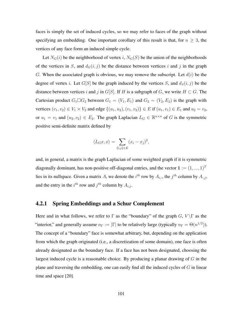
faces is simply the set of induced cycles, so we may refer to faces of the graph without

specifying an embedding. One important corollary of this result is that, for 𝑛 ≥ 3, the

vertices of any face form an induced simple cycle.

Let 𝑁𝐺(𝑖) be the neighborhood of vertex 𝑖, 𝑁𝐺(𝑆) be the union of the neighborhoods

of the vertices in 𝑆, and 𝑑𝐺(𝑖, 𝑗) be the distance between vertices 𝑖 and 𝑗 in the graph

𝐺. When the associated graph is obvious, we may remove the subscript. Let 𝑑(𝑖) be the

degree of vertex 𝑖. Let 𝐺[𝑆] be the graph induced by the vertices 𝑆, and 𝑑𝑆(𝑖, 𝑗) be the

distance between vertices 𝑖 and 𝑗 in 𝐺[𝑆]. If 𝐻 is a subgraph of 𝐺, we write 𝐻 ⊂ 𝐺. The

Cartesian product 𝐺1𝐺2 between 𝐺1 = (𝑉1, 𝐸1) and 𝐺2 = (𝑉2, 𝐸2) is the graph with

vertices (𝑣1, 𝑣2) ∈ 𝑉1 × 𝑉2 and edge (𝑢1, 𝑢2), (𝑣1, 𝑣2) ∈ 𝐸 if (𝑢1, 𝑣1) ∈ 𝐸1 and 𝑢2 = 𝑣2,

or 𝑢1 = 𝑣1 and (𝑢2, 𝑣2) ∈ 𝐸2. The graph Laplacian 𝐿𝐺 ∈ R𝑛×𝑛 of 𝐺 is the symmetric

positive semi-definite matrix defined by

⟨𝐿𝐺𝑥, 𝑥⟩ =∑

𝑖,𝑗∈𝐸

(𝑥𝑖 − 𝑥𝑗)2,

and, in general, a matrix is the graph Laplacian of some weighted graph if it is symmetric

diagonally dominant, has non-positive off-diagonal entries, and the vector 1 := (1, ..., 1)𝑇

lies in its nullspace. Given a matrix 𝐴, we denote the 𝑖𝑡ℎ row by 𝐴𝑖,·, the 𝑗𝑡ℎ column by 𝐴·,𝑗 ,

and the entry in the 𝑖𝑡ℎ row and 𝑗𝑡ℎ column by 𝐴𝑖,𝑗 .

4.2.1 Spring Embeddings and a Schur Complement

Here and in what follows, we refer to Γ as the “boundary” of the graph 𝐺, 𝑉 ∖Γ as the

“interior,” and generally assume 𝑛Γ := |Γ| to be relatively large (typically 𝑛Γ = Θ(𝑛1/2)).

The concept of a “boundary” face is somewhat arbitrary, but, depending on the application

from which the graph originated (i.e., a discretization of some domain), one face is often

already designated as the boundary face. If a face has not been designated, choosing the

largest induced cycle is a reasonable choice. By producing a planar drawing of 𝐺 in the

plane and traversing the embedding, one can easily find all the induced cycles of 𝐺 in linear

time and space [20].

101

Without loss of generality, suppose that Γ = 𝑛− 𝑛Γ + 1, ..., 𝑛. A matrix 𝑋 ∈ R𝑛×2 is

said to be a planar embedding of 𝐺 if the drawing of 𝐺 using straight lines and with vertex 𝑖

located at coordinates 𝑋𝑖,· for all 𝑖 ∈ 𝑉 is a planar drawing. A matrix 𝑋Γ ∈ R𝑛Γ×2 is said

to be a convex embedding of Γ if the embedding is planar and every point is an extreme

point of the convex hull conv([𝑋Γ]𝑖,·𝑛Γ𝑖=1). Tutte’s spring embedding theorem states that if

𝑋Γ is a convex embedding of Γ, then the system of equations

𝑋𝑖,· =

⎧⎪⎨⎪⎩1

𝑑(𝑖)

∑𝑗∈𝑁(𝑖) 𝑋𝑗,· 𝑖 = 1, ..., 𝑛− 𝑛Γ

[𝑋Γ]𝑖−(𝑛−𝑛Γ),· 𝑖 = 𝑛− 𝑛Γ + 1, ..., 𝑛

has a unique solution 𝑋 , and this solution is a planar embedding of 𝐺 [116].

We can write both the Laplacian and embedding of 𝐺 in block-notation, differentiating

between interior and boundary vertices as follows:

𝐿𝐺 =

⎛⎝𝐿𝑜 + 𝐷𝑜 −𝐴𝑜,Γ

−𝐴𝑇𝑜,Γ 𝐿Γ + 𝐷Γ

⎞⎠ ∈ R𝑛×𝑛, 𝑋 =

⎛⎝𝑋𝑜

𝑋Γ

⎞⎠ ∈ R𝑛×2,

where 𝐿𝑜, 𝐷𝑜 ∈ R(𝑛−𝑛Γ)×(𝑛−𝑛Γ), 𝐿Γ, 𝐷Γ ∈ R𝑛Γ×𝑛Γ , 𝐴𝑜,Γ ∈ R(𝑛−𝑛Γ)×𝑛Γ , 𝑋𝑜 ∈ R(𝑛−𝑛Γ)×2,

𝑋Γ ∈ R𝑛Γ×2, and 𝐿𝑜 and 𝐿Γ are the Laplacians of 𝐺[𝑉 ∖Γ] and 𝐺[Γ], respectively. Using

block notation, the system of equations for the Tutte spring embedding of some convex

embedding 𝑋Γ is given by

𝑋𝑜 = (𝐷𝑜 + 𝐷[𝐿𝑜])−1[(𝐷[𝐿𝑜]− 𝐿𝑜)𝑋𝑜 + 𝐴𝑜,Γ𝑋Γ],

where 𝐷[𝐴] is the diagonal matrix with diagonal entries given by the diagonal of 𝐴. The

unique solution to this system is

𝑋𝑜 = (𝐿𝑜 + 𝐷𝑜)−1𝐴𝑜,Γ𝑋Γ.

We note that this choice of 𝑋𝑜 not only guarantees a planar embedding of 𝐺, but also

102

minimizes Hall’s energy, namely,

arg min𝑋𝑜

ℎ(𝑋) = (𝐿𝑜 + 𝐷𝑜)−1𝐴𝑜,Γ𝑋Γ,

where ℎ(𝑋) := Tr(𝑋𝑇𝐿𝑋) (see [62] for more on Hall’s energy).

While Tutte’s theorem is a very powerful result, guaranteeing that, given a convex

embedding of any face, the energy minimizing embedding of the remaining vertices results

in a planar embedding, it gives no direction as to how this outer face should be embedded.

We consider embeddings of the boundary that minimize Hall’s energy, given some

normalization. We consider embeddings that satisfy 𝑋𝑇Γ𝑋Γ = 𝐼 and 𝑋𝑇

Γ 1 = 0, though

other normalizations, such as 𝑋𝑇𝑋 = 𝐼 and 𝑋𝑇1 = 0, would be equally appropriate. The

analysis that follows in this section can be readily applied to this alternate normalization,

but it does require the additional step of verifying a norm equivalence between 𝑉 and Γ

for the harmonic extension of low energy vectors, which can be produced relatively easily

for the class of graphs considered in Subsection 4.2.2. In addition, alternate normalization

techniques, such as the introduction of negative weights on the boundary cycle, can also

be considered. Let 𝒳 be the set of all planar embeddings 𝑋Γ that satisfy 𝑋𝑇Γ𝑋Γ = 𝐼 ,

𝑋𝑇Γ 1 = 0, and for which the spring embedding 𝑋 with 𝑋𝑜 = (𝐿𝑜 + 𝐷𝑜)

−1𝐴𝑜,Γ𝑋Γ is planar.

We consider the optimization problem

min ℎ(𝑋) 𝑠.𝑡. 𝑋Γ ∈ cl(𝒳 ), (4.1)

where cl(·) is the closure of a set. The set 𝒳 is not closed, and the minimizer of (4.1) may

be non-planar, but must be arbitrarily close to a planar embedding. The normalizations

𝑋𝑇Γ 1 = 0 and 𝑋𝑇

Γ𝑋Γ = 𝐼 ensure that the solution does not degenerate into a single

point or line. In what follows we are primarily concerned with approximately solving this

optimization problem and connecting this problem to the Schur complement of 𝐿𝐺 with

respect to 𝑉 ∖Γ. It is unclear whether there exists an efficient algorithm to solve (4.1) exactly

or if the associated decision problem is NP-hard. If (4.1) is NP-hard, it seems rather difficult

to verify that this is indeed the case.

103

A Schur Complement

Given some choice of 𝑋Γ, by Tutte’s theorem the minimum value of ℎ(𝑋) is attained when

𝑋𝑜 = (𝐿𝑜 + 𝐷𝑜)−1𝐴𝑜,Γ𝑋Γ, and given by

Tr

⎡⎣([(𝐿𝑜 + 𝐷𝑜)−1𝐴𝑜,Γ𝑋Γ]𝑇 𝑋𝑇

Γ

)⎛⎝𝐿𝑜 + 𝐷𝑜 −𝐴𝑜,Γ

−𝐴𝑇𝑜,Γ 𝐿Γ + 𝐷Γ

⎞⎠⎛⎝(𝐿𝑜 + 𝐷𝑜)−1𝐴𝑜,Γ𝑋Γ

𝑋Γ

⎞⎠⎤⎦= Tr

(𝑋𝑇

Γ

[𝐿Γ + 𝐷Γ − 𝐴𝑇

𝑜,Γ(𝐿𝑜 + 𝐷𝑜)−1𝐴𝑜,Γ

]𝑋Γ

)= Tr

(𝑋𝑇

Γ 𝑆Γ𝑋Γ

),

where 𝑆Γ is the Schur complement of 𝐿𝐺 with respect to 𝑉 ∖Γ,

𝑆Γ = 𝐿Γ + 𝐷Γ − 𝐴𝑇𝑜,Γ(𝐿𝑜 + 𝐷𝑜)

−1𝐴𝑜,Γ.

For this reason, we can instead consider the optimization problem

min ℎΓ(𝑋Γ) 𝑠.𝑡. 𝑋Γ ∈ cl(𝒳 ), (4.2)

where

ℎΓ(𝑋Γ) := Tr(𝑋𝑇

Γ 𝑆Γ𝑋Γ

).

Therefore, if the minimal two non-trivial eigenvectors of 𝑆Γ produce a planar spring

embedding, then this is the exact solution of (4.2). However, a priori, there is no reason to

think that this drawing would be planar. It turns out that, for a large class of graphs with

some macroscopic structure, this is often the case (see, for example, Figures 4-1 and 4-2),

and, in the rare instance that it is not, through a spectral equivalence result, a low energy

planar and convex embedding of the boundary always exists. This fact follows from the

spectral equivalence of 𝑆Γ and 𝐿1/2Γ , which is shown in Subsection 4.2.2.

First, we present a number of basic properties of the Schur complement of a graph

Laplacian. For more information on the Schur complement, we refer the reader to [18, 40,

134].

104

Proposition 8. Let 𝐺 = (𝑉,𝐸), 𝑛 = |𝑉 |, be a graph and 𝐿𝐺 ∈ R𝑛×𝑛 the associated graph

Laplacian. Let 𝐿𝐺 and vectors 𝑣 ∈ R𝑛 be written in block form

𝐿(𝐺) =

⎛⎝𝐿11 𝐿12

𝐿21 𝐿22

⎞⎠ , 𝑣 =

⎛⎝𝑣1

𝑣2

⎞⎠ ,

where 𝐿22 ∈ R𝑚×𝑚, 𝑣2 ∈ R𝑚, and 𝐿12 = 0. Then

(1) 𝑆 = 𝐿22 − 𝐿21𝐿−111 𝐿12 is a graph Laplacian,

(2)∑𝑚

𝑖=1(𝑒𝑇𝑖 𝐿221𝑚)𝑒𝑖𝑒

𝑇𝑖 − 𝐿21𝐿

−111 𝐿12 is a graph Laplacian,

(3) ⟨𝑆𝑤,𝑤⟩ = inf⟨𝐿𝑣, 𝑣⟩|𝑣2 = 𝑤.

Proof. Let 𝑃 =

⎛⎝−𝐿−111 𝐿12

𝐼

⎞⎠ ∈ R𝑛×𝑚. Then

𝑃 𝑇𝐿𝑃 =(−𝐿21𝐿

−111 𝐼

)⎛⎝𝐿11 𝐿12

𝐿21 𝐿22

⎞⎠⎛⎝−𝐿−111 𝐿12

𝐼

⎞⎠ = 𝐿22 − 𝐿21𝐿−111 𝐿12 = 𝑆.

Because 𝐿111𝑛−𝑚 +𝐿121𝑚 = 0, we have 1𝑛−𝑚 = −𝐿−111 𝐿121𝑚. Therefore 𝑃1𝑚 = 1𝑛, and,

as a result,

𝑆1𝑚 = 𝑃 𝑇𝐿𝑃1𝑚 = 𝑃 𝑇𝐿1𝑛 = 𝑃 𝑇0 = 0.

In addition,[𝑚∑𝑖=1

(𝑒𝑇𝑖 𝐿221𝑚)𝑒𝑖𝑒𝑇𝑖 − 𝐿21𝐿

−111 𝐿12

]1𝑚 =

[ 𝑚∑𝑖=1

(𝑒𝑇𝑖 𝐿221𝑚)𝑒𝑖𝑒𝑇𝑖 − 𝐿22

]1𝑚 + 𝑆1𝑚

=𝑚∑𝑖=1

(𝑒𝑇𝑖 𝐿221𝑚)𝑒𝑖 − 𝐿221𝑚

=

[ 𝑚∑𝑖=1

𝑒𝑖𝑒𝑇𝑖 − 𝐼𝑚

]𝐿221𝑚 = 0.

𝐿11 is an M-matrix, so 𝐿−111 is a non-negative matrix. 𝐿21𝐿

−111 𝐿12 is the product of three non-

negative matrices, and so must also be non-negative. Therefore, the off-diagonal entries of

105

𝑆 and∑𝑚

𝑖=1(𝑒𝑇𝑖 𝐿221)𝑒𝑖𝑒

𝑇𝑖 − 𝐿21𝐿

−111 𝐿12 are non-positive, and so both are graph Laplacians.

Consider

⟨𝐿𝑣, 𝑣⟩ = ⟨𝐿11𝑣1, 𝑣1⟩+ 2⟨𝐿12𝑣2, 𝑣1⟩+ ⟨𝐿22𝑣2, 𝑣2⟩,

with 𝑣2 fixed. Because 𝐿11 is symmetric positive definite, the minimum occurs when

𝜕

𝜕𝑣1⟨𝐿𝑣, 𝑣⟩ = 2𝐿11𝑣1 + 2𝐿12𝑣2 = 0.

Setting 𝑣1 = −𝐿−111 𝐿12𝑣2, the desired result follows.

The above result illustrates that the Schur complement Laplacian 𝑆Γ is the sum of two

Laplacians 𝐿Γ and 𝐷Γ−𝐴𝑇𝑜,Γ(𝐿𝑜 +𝐷𝑜)

−1𝐴𝑜,Γ, where the first is the Laplacian of 𝐺[Γ], and

the second is a Laplacian representing the dynamics of the interior.

An Algorithm

Given the above analysis for 𝑆Γ, and assuming a spectral equivalence result of the form

1

𝑐1⟨𝐿1/2

Γ 𝑥, 𝑥⟩ ≤ ⟨𝑆Γ𝑥, 𝑥⟩ ≤ 𝑐2 ⟨𝐿1/2Γ 𝑥, 𝑥⟩, (4.3)

for all 𝑥 ∈ R𝑛Γ and some constants 𝑐1 and 𝑐2 that are not too large, we can construct a simple

algorithm for producing a spring embedding. Constants 𝑐1 and 𝑐2 can be computed explicitly

using the results of Subsection 4.2.2, and are reasonably sized if the graph resembles a

discretization of some planar domain (i.e., a graph that satisfies the conditions of Theorem

15). Given these two facts, a very natural algorithm consists of the following steps. First we

compute the two eigenvectors corresponding to the two minimal non-trivial eigenvalues of

the Schur complement 𝑆Γ. If these two eigenvectors produce a planar embedding, we are

done, and have solved the optimization problem (4.2) exactly. Depending on the structure

of the graph, this may often be the case. For instance, this occurs for the graphs in Figures

4-1 and 4-2, and the numerical results of [124] confirm that this also occurs often for

discretizations of circular and rectangular domains. If this is not the case, then we consider

106

Algorithm 3 A Schur Complement-Based Spring Embedding Algorithm

function SchurSPRING(𝐺,Γ)Compute the two minimal non-trivial eigenpairs 𝑋𝑎𝑙𝑔 ∈ R𝑛Γ×2 of 𝑆Γ

if spring embedding of 𝑋𝑎𝑙𝑔 is non-planar then𝑋𝑛𝑒𝑤 ←

2𝑛Γ

(cos 2𝜋𝑗

𝑛Γ, sin 2𝜋𝑗

𝑛Γ

)𝑛Γ

𝑗=1; gap← 1

while spring embedding of 𝑋𝑛𝑒𝑤 is planar, gap > 0 do ← smooth(𝑋𝑛𝑒𝑤); 𝑋𝑎𝑙𝑔 ← 𝑋𝑛𝑒𝑤

← − 11𝑇 /𝑛Γ

Solve [𝑇 ]𝑄 = 𝑄Λ, 𝑄 orthogonal, Λ diagonal; set 𝑋𝑛𝑒𝑤 ← 𝑄Λ−1/2

gap← ℎΓ(𝑋𝑎𝑙𝑔)− ℎΓ(𝑋𝑛𝑒𝑤)end while

end ifReturn 𝑋𝑎𝑙𝑔

end function

the boundary embedding

[𝑋𝐶 ]𝑗,· =2

𝑛Γ

(cos

2𝜋𝑗

𝑛Γ

, sin2𝜋𝑗

𝑛Γ

), 𝑗 = 1, ..., 𝑛Γ,

namely, the embedding of the two minimal non-trivial eigenvectors of 𝐿1/2Γ . This choice

of boundary is convex and planar, and so the associated spring embedding is planar. By

spectral equivalence,

ℎΓ(𝑋𝐶) ≤ 4𝑐2 sin𝜋

𝑛Γ

≤ 𝑐1𝑐2 min𝑋Γ∈cl(𝒳 )

ℎΓ(𝑋Γ),

and therefore, this algorithm already produces a 𝑐1𝑐2 approximation guarantee for (4.2).

The choice of 𝑋𝐶 can often be improved, and a natural technique consists of smoothing

𝑋𝐶 using 𝑆Γ and renormalizing until either the resulting drawing is no longer planar or the

objective value no longer decreases. We describe this procedure in Algorithm 3.

We now discuss some of the finer details of the SchurSPRING(𝐺,Γ) algorithm (Algo-

rithm 3). Determining whether a drawing is planar can be done in near-linear time using

the sweep line algorithm [102]. Also, in practice, it is advisable to replace conditions of the

form gap > 0 in Algorithm 3 by gap > tol for some small value of tol, in order to ensure

that the algorithm terminates after some finite number of steps. For a reasonable choice of

107

smoother, a constant tolerance, and 𝑛Γ = Θ(𝑛1/2), the SchurSPRING(𝐺,Γ) algorithm has

complexity near-linear in 𝑛. The main cost of this procedure is due to the computations that

involve 𝑆Γ.

The SchurSPRING(𝐺,Γ) algorithm requires the repeated application of 𝑆Γ or 𝑆−1Γ in

order to compute the minimal eigenvectors of 𝑆Γ and also to perform smoothing. The Schur

complement 𝑆Γ is a dense matrix and requires the inversion of a (𝑛−𝑛Γ)× (𝑛−𝑛Γ) matrix,

but can be represented as the composition of functions of sparse matrices. In practice,

𝑆Γ should never be formed explicitly. Rather, the operation of applying 𝑆Γ to a vector 𝑥

should occur in two steps. First, the sparse Laplacian system (𝐿𝑜 + 𝐷𝑜)𝑦 = 𝐴𝑜,Γ𝑥 should

be solved for 𝑦, and then the product 𝑆𝑥 is given by 𝑆Γ𝑥 = (𝐿Γ + 𝐷Γ)𝑥 − 𝐴𝑇𝑜,Γ𝑦. Each

application of 𝑆Γ is therefore an (𝑛) procedure (using a nearly-linear time Laplacian

solver). The application of the inverse 𝑆−1Γ defined on the subspace 𝑥 | ⟨𝑥,1⟩ = 0 also

requires the solution of a Laplacian system. As noted in [130], the action of 𝑆−1Γ on a vector

𝑥 ∈ 𝑥 | ⟨𝑥,1⟩ = 0 is given by

𝑆−1Γ 𝑥 =

(0 𝐼

)⎛⎝𝐿𝑜 + 𝐷𝑜 −𝐴𝑜,Γ

−𝐴𝑇𝑜,Γ 𝐿Γ + 𝐷Γ

⎞⎠−1⎛⎝0

𝑥

⎞⎠ ,

as verified by the computation

𝑆Γ

[𝑆−1Γ 𝑥]

= 𝑆Γ

(0 𝐼

)⎡⎣⎛⎝ 𝐼 0

−𝐴𝑇𝑜,Γ(𝐿𝑜 + 𝐷𝑜)

−1 𝐼

⎞⎠⎛⎝𝐿𝑜 + 𝐷𝑜 −𝐴𝑜,Γ

0 𝑆Γ

⎞⎠⎤⎦−1⎛⎝0

𝑥

⎞⎠= 𝑆Γ

(0 𝐼

)⎛⎝𝐿𝑜 + 𝐷𝑜 −𝐴𝑜,Γ

0 𝑆Γ

⎞⎠−1⎛⎝ 𝐼 0

𝐴𝑇𝑜,Γ(𝐿𝑜 + 𝐷𝑜)

−1 𝐼

⎞⎠⎛⎝0

𝑥

⎞⎠= 𝑆Γ

(0 𝐼

)⎛⎝𝐿𝑜 + 𝐷𝑜 −𝐴𝑜,Γ

0 𝑆Γ

⎞⎠−1⎛⎝0

𝑥

⎞⎠ = 𝑥.

Given that the application of 𝑆−1Γ has the same complexity as an application 𝑆Γ, the inverse

power method is naturally preferred over the shifted power method for both smoothing and

the computation of low energy eigenvectors.

108

4.2.2 A Discrete Trace Theorem and Spectral Equivalence

The main result of this subsection takes classical trace theorems from the theory of partial

differential equations and extends them to a class of planar graphs. However, for our

purposes, we require a stronger form of trace theorem, one between energy semi-norms

(i.e., no ℓ2 term), which we refer to as “energy-only” trace theorems. These energy-only

trace theorems imply their classical variants with ℓ2 terms almost immediately. We then

use these new results to prove the spectral equivalence of 𝑆Γ and 𝐿1/2Γ for the class of

graphs under consideration. This class of graphs is rigorously defined below, but includes

planar three-connected graphs that have some regular structure (such as graphs of finite

element discretizations). For the sake of space and readibility, a number of the results of

this subsection are stated for arbitrary constants, or constants larger than necessary. More

complicated proofs with explicit constants (or, in some cases, improved constants) can be

found in [124]. We begin by formally describing a classical trace theorem.

Let Ω ⊂ R𝑑 be a domain with boundary Γ = 𝛿Ω that, locally, is a graph of a Lipschitz

function. 𝐻1(Ω) is the Sobolev space of square integrable functions with square integrable

weak gradient, with norm

‖𝑢‖21,Ω = ‖∇𝑢‖2𝐿2(Ω) + ‖𝑢‖2𝐿2(Ω), where ‖𝑢‖2𝐿2(Ω) =

∫Ω

𝑢2 𝑑𝑥.

Let

‖𝜙‖21/2,Γ = ‖𝜙‖2𝐿2(Γ)+

∫∫Γ×Γ

(𝜙(𝑥)− 𝜙(𝑦))2

|𝑥− 𝑦|𝑑𝑑𝑥 𝑑𝑦

for functions defined on Γ, and denote by 𝐻1/2(Γ) the Sobolev space of functions defined on

the boundary Γ for which ‖ · ‖1/2,Γ is finite. The trace theorem for functions in 𝐻1(Ω) is one

of the most important and frequently used trace theorems in the theory of partial differential

equations. More general results for traces on boundaries of Lipschitz domains, which

involve 𝐿𝑝 norms and fractional derivatives, are due to E. Gagliardo [42] (see also [24]).

Gagliardo’s theorem, when applied to the case of 𝐻1(Ω) and 𝐻1/2(Γ), states that if Ω ⊂ R𝑑

109

is a Lipschitz domain, then the norm equivalence

‖𝜙‖1/2,Γ h inf‖𝑢‖1,Ω𝑢|Γ = 𝜙

holds (the right hand side is indeed a norm on 𝐻1/2(Γ)). These results are key tools in

proving a priori estimates on the Dirichlet integral of functions with given data on the

boundary of a domain Ω. Roughly speaking, a trace theorem gives a bound on the energy

of a harmonic function via norm of the trace of the function on Γ = 𝜕Ω. In addition to

the classical references given above, further details on trace theorems and their role in the

analysis of PDEs (including the case of Lipschitz domains) can be found in [77, 87]. There

are several analogues of this theorem for finite element spaces (finite dimensional subspaces

of 𝐻1(Ω)). For instance, in [86] it is shown that the finite element discretization of the

Laplace-Beltrami operator on the boundary to the one-half power provides a norm which is

equivalent to the 𝐻1/2(Γ)-norm. Here we prove energy-only analogues of the classical trace

theorem for graphs (𝐺,Γ) ∈ 𝒢𝑛, using energy semi-norms

|𝑢|2𝐺 = ⟨𝐿𝐺𝑢, 𝑢⟩ and |𝜙|2Γ =∑𝑝,𝑞∈Γ,𝑝<𝑞

(𝜙(𝑝)− 𝜙(𝑞))2

𝑑2𝐺(𝑝, 𝑞).

The energy semi-norm | · |𝐺 is a discrete analogue of ‖∇𝑢‖𝐿2(Ω), and the boundary

semi-norm | · |Γ is a discrete analogue of the quantity∫∫

Γ×Γ(𝜙(𝑥)−𝜙(𝑦))2

|𝑥−𝑦|2 𝑑𝑥 𝑑𝑦. In addition,

by connectivity, | · |𝐺 and | · |Γ are norms on the quotient space orthogonal to 1. We aim to

prove that for any 𝜙 ∈ R𝑛Γ ,

1

𝑐1|𝜙|Γ ≤ min

𝑢|Γ=𝜙|𝑢|𝐺 ≤ 𝑐2 |𝜙|Γ

for some constants 𝑐1, 𝑐2 that do not depend on 𝑛Γ, 𝑛. We begin by proving these results for

a simple class of graphs, and then extend our analysis to more general graphs. Some of the

proofs of the below results are rather technical, and are omitted for the sake of readibility

and space.

110

Trace Theorems for a Simple Class of Graphs

Let 𝐺𝑘,ℓ = 𝐶𝑘𝑃ℓ be the Cartesian product of the 𝑘 vertex cycle 𝐶𝑘 and the ℓ vertex path 𝑃ℓ,

where 4ℓ < 𝑘 < 2𝑐ℓ for some constant 𝑐 ∈ N. The lower bound 4ℓ < 𝑘 is arbitrary in some

sense, but is natural, given that the ratio of boundary length to in-radius of a convex region is

at least 2𝜋. Vertex (𝑖, 𝑗) in 𝐺𝑘,ℓ corresponds to the product of 𝑖 ∈ 𝐶𝑘 and 𝑗 ∈ 𝑃ℓ, 𝑖 = 1, ..., 𝑘,

𝑗 = 1, ..., ℓ. The boundary of 𝐺𝑘,ℓ is defined to be Γ = (𝑖, 1)𝑘𝑖=1. Let 𝑢 ∈ R𝑘×ℓ and

𝜙 ∈ R𝑘 be functions on 𝐺𝑘,ℓ and Γ, respectively, with 𝑢[(𝑖, 𝑗)] denoted by 𝑢𝑖,𝑗 and 𝜙[(𝑖, 1)]

denoted by 𝜙𝑖. For the remainder of the section, we consider the natural periodic extension

of the vertices (𝑖, 𝑗) and the functions 𝑢𝑖,𝑗 and 𝜙𝑖 to the indices 𝑖 ∈ Z. In particular, if

𝑖 ∈ 1, ..., 𝑘, then (𝑖, 𝑗) := (𝑖*, 𝑗), 𝜙𝑖 := 𝜙𝑖* , and 𝑢𝑖,𝑗 := 𝑢𝑖*,𝑗 , where 𝑖* ∈ 1, ..., 𝑘 and

𝑖* = 𝑖 mod 𝑘. Let 𝐺*𝑘,ℓ be the graph resulting from adding to 𝐺𝑘,ℓ all edges of the form

(𝑖, 𝑗), (𝑖− 1, 𝑗 + 1) and (𝑖, 𝑗), (𝑖 + 1, 𝑗 + 1), 𝑖 = 1, ..., 𝑘, 𝑗 = 1, ..., ℓ− 1. We provide

a visual example of 𝐺𝑘,ℓ and 𝐺*𝑘,ℓ in Figure 4-3. First, we prove a trace theorem for 𝐺𝑘,ℓ.

The proof of the trace theorem consists of two lemmas. Lemma 10 shows that the discrete

trace operator is bounded, and Lemma 11 shows that it has a continuous right inverse. Taken

together, these lemmas imply our desired result for 𝐺𝑘,ℓ. We then extend this result to all

graphs 𝐻 satisfying 𝐺𝑘,ℓ ⊂ 𝐻 ⊂ 𝐺*𝑘,ℓ.

Lemma 10. Let 𝐺 = 𝐺𝑘,ℓ, 4ℓ < 𝑘 < 2𝑐ℓ, 𝑐 ∈ N, with boundary Γ = (𝑖, 1)𝑘𝑖=1. For any

𝑢 ∈ R𝑘×ℓ, the vector 𝜙 = 𝑢|Γ satisfies |𝜙|Γ ≤ 4√𝑐 |𝑢|𝐺.

Proof. We can decompose 𝜙𝑝+ℎ − 𝜙ℎ into a sum of differences, given by

𝜙𝑝+ℎ − 𝜙𝑝 =𝑠−1∑𝑖=1

𝑢𝑝+ℎ,𝑖 − 𝑢𝑝+ℎ,𝑖+1 +ℎ∑

𝑖=1

𝑢𝑝+𝑖,𝑠 − 𝑢𝑝+𝑖−1,𝑠 +𝑠−1∑𝑖=1

𝑢𝑝,𝑠−𝑖+1 − 𝑢𝑝,𝑠−𝑖,

111

where 𝑠 =⌈ℎ𝑐

⌉is a function of ℎ. By Cauchy-Schwarz,

𝑘∑𝑝=1

⌊𝑘/2⌋∑ℎ=1

(𝜙𝑝+ℎ − 𝜙𝑝

ℎ

)2

≤ 3𝑘∑

𝑝=1

⌊𝑘/2⌋∑ℎ=1

(1

ℎ

𝑠−1∑𝑖=1

𝑢𝑝+ℎ,𝑖 − 𝑢𝑝+ℎ,𝑖+1

)2

+ 3𝑘∑

𝑝=1

⌊𝑘/2⌋∑ℎ=1

(1

ℎ

ℎ∑𝑖=1

𝑢𝑝+𝑖,𝑠 − 𝑢𝑝+𝑖−1,𝑠

)2

+ 3𝑘∑

𝑝=1

⌊𝑘/2⌋∑ℎ=1

(1

ℎ

𝑠−1∑𝑖=1

𝑢𝑝,𝑠−𝑖+1 − 𝑢𝑝,𝑠−𝑖

)2

.

We bound the first and the second term separately. The third term is identical to the first.

Using Hardy’s inequality [50, Theorem 326], we can bound the first term by

𝑘∑𝑝=1

⌊𝑘/2⌋∑ℎ=1

(1

ℎ

𝑠−1∑𝑖=1

𝑢𝑝,𝑖 − 𝑢𝑝,𝑖+1

)2

=𝑘∑

𝑝=1

ℓ∑𝑠=1

(1

𝑠

𝑠−1∑𝑖=1

𝑢𝑝,𝑖 − 𝑢𝑝,𝑖+1

)2 ∑ℎ:⌈ℎ/𝑐⌉=𝑠1≤ℎ≤⌊𝑘/2⌋

𝑠2

ℎ2

≤ 4𝑘∑

𝑝=1

ℓ−1∑𝑠=1

(𝑢𝑝,𝑠 − 𝑢𝑝,𝑠+1

)2 ∑ℎ:⌈ℎ/𝑐⌉=𝑠1≤ℎ≤⌊𝑘/2⌋

𝑠2

ℎ2.

We have

∑ℎ:⌈ℎ/𝑐⌉=𝑠1≤ℎ≤⌊𝑘/2⌋

𝑠2

ℎ2≤ 𝑠2

𝑐𝑠∑𝑖=𝑐(𝑠−1)+1

1

𝑖2≤ 𝑠2(𝑐− 1)

(𝑐(𝑠− 1) + 1)2≤ 4(𝑐− 1)

(𝑐 + 1)2≤ 1

2

for 𝑠 ≥ 2 (𝑐 ≥ 3, by definition), and for 𝑠 = 1,

∑ℎ:⌈ℎ/𝑐⌉=11≤ℎ≤⌊𝑘/2⌋

1

ℎ2≤

∞∑𝑖=1

1

𝑖2=

𝜋2

6.

112

(a) 𝐺16,3 = 𝐶16𝑃3 (b) 𝐺*16,3

Figure 4-3: A visual example of 𝐺𝑘,ℓ and 𝐺*𝑘,ℓ for 𝑘 = 16, ℓ = 3. The boundary Γ is given

by the outer (or, by symmetry, inner) cycle.

Therefore, we can bound the first term by

𝑘∑𝑝=1

⌊𝑘/2⌋∑ℎ=1

(1

ℎ

𝑠−1∑𝑖=1

𝑢𝑝,𝑖 − 𝑢𝑝,𝑖+1

)2

≤ 2𝜋2

3

𝑘∑𝑝=1

ℓ−1∑𝑠=1

(𝑢𝑝,𝑠 − 𝑢𝑝,𝑠+1

)2.

For the second term, we have

𝑘∑𝑝=1

⌊𝑘/2⌋∑ℎ=1

(1

ℎ

ℎ∑𝑖=1

𝑢𝑝+𝑖,𝑠 − 𝑢𝑝+𝑖−1,𝑠

)2

≤𝑘∑

𝑝=1

⌊𝑘/2⌋∑ℎ=1

1

ℎ

ℎ∑𝑖=1

(𝑢𝑝+𝑖,𝑠 − 𝑢𝑝+𝑖−1,𝑠

)2≤ 𝑐

𝑘∑𝑝=1

ℓ∑𝑠=1

(𝑢𝑝+1,𝑠 − 𝑢𝑝,𝑠

)2.

Combining these bounds produces the result |𝜙|2Γ ≤ max4𝜋2, 3𝑐 |𝑢|2𝐺. Noting that 𝑐 ≥ 3

gives the desired result.

In order to show that the discrete trace operator has a continuous right inverse, we need

to produce a provably low-energy extension of an arbitrary function on Γ. Let

𝑎 =1

𝑘

𝑘∑𝑝=1

𝜙𝑝 and 𝑎𝑖,𝑗 =1

2𝑗 − 1

𝑗−1∑ℎ=1−𝑗

𝜙𝑖+ℎ.

113

We consider the extension

𝑢𝑖,𝑗 =𝑗 − 1

ℓ− 1𝑎 +

(1− 𝑗 − 1

ℓ− 1

)𝑎𝑖,𝑗. (4.4)

The proof of following inverse result for the discrete trace operator is similar in technique

to that of Lemma 10, but significantly more involved.

Lemma 11. Let 𝐺 = 𝐺𝑘,ℓ, 4ℓ < 𝑘 < 2𝑐ℓ, 𝑐 ∈ N, with boundary Γ = (𝑖, 1)𝑘𝑖=1. For any

𝜙 ∈ R𝑘, the vector 𝑢 defined by (4.4) satisfies |𝑢|𝐺 ≤ 5√𝑐 |𝜙|Γ.

Proof. We can decompose |𝑢|2𝐺 into two parts, namely,

|𝑢|2𝐺 =𝑘∑

𝑖=1

ℓ∑𝑗=1

(𝑢𝑖+1,𝑗 − 𝑢𝑖,𝑗)2 +

𝑘∑𝑖=1

ℓ−1∑𝑗=1

(𝑢𝑖,𝑗+1 − 𝑢𝑖,𝑗)2.

We bound each sum separately, beginning with the first. We have

𝑢𝑖+1,𝑗 − 𝑢𝑖,𝑗 =

(1− 𝑗 − 1

ℓ− 1

)(𝑎𝑖+1,𝑗 − 𝑎𝑖,𝑗) =

(1− 𝑗 − 1

ℓ− 1

)𝜙𝑖+𝑗 − 𝜙𝑖+1−𝑗

2𝑗 − 1.

Squaring both sides and noting that 4ℓ < 𝑘, we have

𝑘∑𝑖=1

ℓ∑𝑗=1

(𝑢𝑖+1,𝑗 − 𝑢𝑖,𝑗)2 ≤

𝑘∑𝑖=1

ℓ∑𝑗=1

[𝜙𝑖+𝑗 − 𝜙𝑖+1−𝑗

2𝑗 − 1

]2≤

𝑘∑𝑝=1

2ℓ−1∑ℎ=1

[𝜙𝑝+ℎ − 𝜙𝑝

ℎ

]2≤ |𝜙|2Γ.

We now consider the second sum. Each term can be decomposed as

𝑢𝑖,𝑗+1 − 𝑢𝑖,𝑗 =𝑎− 𝑎𝑖,𝑗ℓ− 1

+

(1− 𝑗

ℓ− 1

)[𝑎𝑖,𝑗+1 − 𝑎𝑖,𝑗],

which leads to the upper bound

𝑘∑𝑖=1

ℓ−1∑𝑗=1

(𝑢𝑖,𝑗+1 − 𝑢𝑖,𝑗)2 ≤ 2

𝑘∑𝑖=1

ℓ−1∑𝑗=1

[𝑎− 𝑎𝑖,𝑗ℓ− 1

]2+ 2

𝑘∑𝑖=1

ℓ−1∑𝑗=1

(𝑎𝑖,𝑗+1 − 𝑎𝑖,𝑗)2.

We estimate the two terms in the previous equation separately, beginning with the first. The

114

difference 𝑎− 𝑎𝑖,𝑗 can be written as

𝑎− 𝑎𝑖,𝑗 =1

𝑘

𝑘∑𝑝=1

𝜙𝑝 −1

2𝑗 − 1

𝑗−1∑ℎ=1−𝑗

𝜙𝑖+ℎ =1

𝑘(2𝑗 − 1)

𝑘∑𝑝=1

𝑗−1∑ℎ=1−𝑗

𝜙𝑝 − 𝜙𝑖+ℎ.

Squaring both sides,

(𝑎− 𝑎𝑖,𝑗)2 =

1

𝑘2(2𝑗 − 1)2

(𝑘∑

𝑝=1

𝑗−1∑ℎ=1−𝑗

𝜙𝑝 − 𝜙𝑖+ℎ

)2

≤ 1

𝑘(2𝑗 − 1)

𝑘∑𝑝=1

𝑗−1∑ℎ=1−𝑗

(𝜙𝑝 − 𝜙𝑖+ℎ)2.

Summing over all 𝑖 and 𝑗 gives

𝑘∑𝑖=1

ℓ−1∑𝑗=1

[𝑎− 𝑎𝑖,𝑗ℓ− 1

]2≤ 1

(ℓ− 1)2

𝑘∑𝑖=1

ℓ−1∑𝑗=1

1

𝑘(2𝑗 − 1)

𝑘∑𝑝=1

𝑗−1∑ℎ=1−𝑗

(𝜙𝑝 − 𝜙𝑖+ℎ)2

=𝑘

4(ℓ− 1)2

ℓ−1∑𝑗=1

1

2𝑗 − 1

𝑗−1∑ℎ=1−𝑗

𝑘∑𝑖,𝑝=1

(𝜙𝑝 − 𝜙𝑖+ℎ)2

𝑘2/4

≤ 𝑘

4(ℓ− 1)|𝜙|2Γ ≤ 𝑐|𝜙|2Γ.

This completes the analysis of the first term. For the second term, we have

𝑎𝑖,𝑗+1 − 𝑎𝑖,𝑗 =1

2𝑗 + 1

[𝜙𝑖+𝑗 + 𝜙𝑖−𝑗 −

2

2𝑗 − 1

𝑗−1∑ℎ=1−𝑗

𝜙𝑖+ℎ

].

Next, we note that𝜙𝑖+𝑗 −

𝜙𝑖

2𝑗 − 1− 2

2𝑗 − 1

𝑗−1∑ℎ=1

𝜙𝑖+ℎ

=

𝜙𝑖+𝑗 − 𝜙𝑖

2𝑗 − 1+ 2

𝑗−1∑ℎ=1

𝜙𝑖+𝑗 − 𝜙𝑖+ℎ

2𝑗 − 1

≤ 2

𝑗−1∑ℎ=0

|𝜙𝑖+𝑗 − 𝜙𝑖+ℎ|2𝑗 − 1

,

115

and, similarly,

𝜙𝑖−𝑗 −

𝜙𝑖

2𝑗 − 1− 2

2𝑗 − 1

𝑗−1∑ℎ=1

𝜙𝑖−ℎ

=

𝜙𝑖−𝑗 − 𝜙𝑖

2𝑗 − 1+ 2

𝑗−1∑ℎ=1

𝜙𝑖−𝑗 − 𝜙𝑖−ℎ

2𝑗 − 1

≤ 2

𝑗−1∑ℎ=0

|𝜙𝑖−𝑗 − 𝜙𝑖−ℎ|2𝑗 − 1

.

Hence,

𝑙−1∑𝑗=1

(𝑎𝑖,𝑗+1 − 𝑎𝑖,𝑗)2 ≤

𝑙−1∑𝑗=1

8

(2𝑗 + 1)2

⎡⎣( 𝑗−1∑ℎ=0

|𝜙𝑖+𝑗 − 𝜙𝑖+ℎ|2𝑗 − 1

)2

+

(𝑗−1∑ℎ=0

|𝜙𝑖−𝑗 − 𝜙𝑖−ℎ|2𝑗 − 1

)2⎤⎦ .

Once we sum over all 𝑖, the sum of the first and second term are identical, and therefore

𝑘∑𝑖=1

𝑙−1∑𝑗=1

(𝑎𝑖,𝑗+1 − 𝑎𝑖,𝑗)2 ≤ 16

𝑘∑𝑖=1

𝑙−1∑𝑗=1

(𝑗−1∑ℎ=0

|𝜙𝑖+𝑗 − 𝜙𝑖+ℎ|(2𝑗 − 1)(2𝑗 + 1)

)2

.

We have

𝑗−1∑ℎ=0

|𝜙𝑖+𝑗 − 𝜙𝑖+ℎ|(2𝑗 − 1)(2𝑗 + 1)

≤ 1

3𝑗

𝑖+𝑗−1∑𝑝=𝑖

|𝜙𝑖+𝑗 − 𝜙𝑝|𝑗

≤ 1

3𝑗

𝑖+𝑗−1∑𝑝=𝑖

|𝜙𝑖+𝑗 − 𝜙𝑝|𝑖 + 𝑗 − 𝑝

,

which implies that

16𝑘∑

𝑖=1

𝑙−1∑𝑗=1

(𝑗−1∑ℎ=0

|𝜙𝑖+𝑗 − 𝜙𝑖+ℎ|(2𝑗 − 1)(2𝑗 + 1)

)2

≤ 16

9

𝑘∑𝑖=1

𝑙−1∑𝑗=1

(1

𝑗

𝑖+𝑗−1∑𝑝=𝑖

|𝜙𝑖+𝑗 − 𝜙𝑝|𝑖 + 𝑗 − 𝑝

)2

≤ 16

9

𝑘+ℓ−1∑𝑞=1

𝑞−1∑𝑚=1

(1

𝑞 −𝑚

𝑞−1∑𝑝=𝑚

|𝜙𝑞 − 𝜙𝑝|𝑞 − 𝑝

)2

,

where 𝑞 = 𝑖+ 𝑗 and 𝑚 = 𝑖. Letting 𝑟 = 𝑞−𝑚, 𝑠 = 𝑞− 𝑝, and using Hardy’s inequality [50,

116

Theorem 326], we obtain

16

9

𝑘+ℓ−1∑𝑞=1

𝑞−1∑𝑚=1

(1

𝑞 −𝑚

𝑞−1∑𝑝=𝑚

|𝜙𝑞 − 𝜙𝑝|𝑞 − 𝑝

)2

=16

9

𝑘+ℓ−1∑𝑞=1

𝑞−1∑𝑟=1

(1

𝑟

𝑟∑𝑠=1

|𝜙𝑞 − 𝜙𝑞−𝑠|𝑠

)2

≤ 64

9

𝑘+ℓ−1∑𝑞=1

𝑞−1∑𝑟=1

[𝜙𝑞 − 𝜙𝑞−𝑟

𝑟

]2

≤ 64

9

𝑘+ℓ−1∑𝑞=1

𝑞−1∑𝑟=1

[𝜙𝑞 − 𝜙𝑞−𝑟

𝑑𝐺((𝑞, 1), (𝑞 − 𝑟, 1)

)]2≤ 256

9|𝜙|2Γ,

where we note that the sum over the indices 𝑞 and 𝑟 consists of some amount of over-

counting, with some terms (𝜙(𝑞) − 𝜙(𝑞 − 𝑟))2 appearing up to four times. Improved

estimates can be obtained by noting that the choice of indexing for Γ is arbitrary (see [124]

for details), but, for the sake of readability, we focus on simplicity over tight constants.

Combining our estimates and noting that 𝑐 ≥ 3, we obtain the desired result

|𝑢|𝐺 ≤

√1 + 2

(𝑐 +

256

9

)|𝜙|Γ =

√2𝑐 +

521

9|𝜙|Γ ≤ 5

√𝑐 |𝜙|Γ.

Combining Lemmas 10 and 11, we obtain our desired trace theorem.

Theorem 12. Let 𝐺 = 𝐺𝑘,ℓ, 4ℓ < 𝑘 < 2𝑐ℓ, 𝑐 ∈ N, with boundary Γ = (𝑖, 1)𝑘𝑖=1. For any

𝜙 ∈ R𝑘,1

4√𝑐|𝜙|Γ ≤ min

𝑢|Γ=𝜙|𝑢|𝐺 ≤ 5

√𝑐 |𝜙|Γ.

With a little more work, we can prove a similar result for a slightly more general class

of graphs. Using Theorem 12, we can almost immediately prove a trace theorem for any

graph 𝐻 satisfying 𝐺𝑘,ℓ ⊂ 𝐻 ⊂ 𝐺*𝑘,ℓ. In fact, Lemma 10 carries over immediately. In order

to prove a new version of Lemma 11, it suffices to bound the energy of 𝑢 on the edges in

117

𝐺*𝑘,ℓ not contained in 𝐺𝑘,ℓ. By Cauchy-Schwarz,

|𝑢|2𝐺* = |𝑢|2𝐺 +𝑘∑

𝑖=1

ℓ−1∑𝑗=1

[(𝑢𝑖,𝑗+1 − 𝑢𝑖−1,𝑗)

2 + (𝑢𝑖,𝑗+1 − 𝑢𝑖+1,𝑗)2

]

≤ 3𝑘∑

𝑖=1

ℓ∑𝑗=1

(𝑢𝑖+1,𝑗 − 𝑢𝑖,𝑗)2 + 2

𝑘∑𝑖=1

ℓ−1∑𝑗=1

(𝑢𝑖,𝑗+1 − 𝑢𝑖,𝑗)2 ≤ 3 |𝑢|2𝐺,

and therefore Corollary 1 follows immediately from Lemmas 10 and 11.

Corollary 1. Let 𝐻 satisfy 𝐺𝑘,ℓ ⊂ 𝐻 ⊂ 𝐺*𝑘,ℓ, 4ℓ < 𝑘 < 2𝑐ℓ, 𝑐 ∈ N, with boundary

Γ = (𝑖, 1)𝑘𝑖=1. For any 𝜙 ∈ R𝑘,

1

4√𝑐|𝜙|Γ ≤ min

𝑢|Γ=𝜙|𝑢|𝐻 ≤ 5

√3𝑐 |𝜙|Γ.

Trace Theorems for General Graphs

In order to extend Corollary 1 to more general graphs, we introduce a graph operation which

is similar in concept to an aggregation (a partition of 𝑉 into connected subsets) in which the

size of aggregates is bounded. In particular, we give the following definition.

Definition 2. The graph 𝐻 , 𝐺𝑘,ℓ ⊂ 𝐻 ⊂ 𝐺*𝑘,ℓ, is said to be an 𝑀 -aggregation of (𝐺,Γ) ∈

𝒢𝑛 if there exists a partition 𝒜 = 𝑎* ∪ 𝑎𝑖,𝑗𝑗=1,...,ℓ𝑖=1,...,𝑘 of 𝑉 (𝐺) satisfying

1. 𝐺[𝑎𝑖,𝑗] is connected and |𝑎𝑖,𝑗| ≤𝑀 for all 𝑖 = 1, ..., 𝑘, 𝑗 = 1, ..., ℓ,

2. Γ ⊂⋃𝑘

𝑖=1 𝑎𝑖,1, and Γ ∩ 𝑎𝑖,1 = ∅ for all 𝑖 = 1, ..., 𝑘,

3. 𝑁𝐺(𝑎*) ⊂ 𝑎* ∪⋃𝑘

𝑖=1 𝑎𝑖,ℓ,

4. the aggregation graph of 𝒜∖𝑎*, given by

(𝒜∖𝑎*, (𝑎𝑖1,𝑗1 , 𝑎𝑖2,𝑗2) |𝑁𝐺(𝑎𝑖1,𝑗1) ∩ 𝑎𝑖2,𝑗2 = 0),

is isomorphic to 𝐻 .

118

(a) graph (𝐺,Γ) (b) partition 𝒜 (c) 𝐺6,2 ⊂ 𝐻 ⊂ 𝐺*6,2

Figure 4-4: An example of an 𝑀 -aggregation. Figure (A) provides a visual representationof a graph 𝐺, with boundary vertices Γ enlarged. Figure (B) shows a partition 𝒜 of 𝐺, inwhich each aggregate (enclosed by dotted lines) has order at most four. The set 𝑎* is denotedby a shaded region. Figure (C) shows the aggregation graph 𝐻 of 𝒜∖𝑎*. The graph 𝐻satisfies 𝐺6,2 ⊂ 𝐻 ⊂ 𝐺*

6,2, and is therefore a 4-aggregation of (𝐺,Γ).

We provide a visual example in Figure 4-4, and later show that this operation applies

to a fairly large class of graphs. However, the 𝑀 -aggregation procedure is not the only

operation for which we can control the behavior of the energy and boundary semi-norms. For

instance, the behavior of our semi-norms under the deletion of some number of edges can be

bounded easily if each edge can be replaced by a path of constant length, and no remaining

edge is contained in more than a constant number of such paths. In addition, the behavior

of these semi-norms under the disaggregation of large degree vertices is also relatively

well-behaved (see [52] for details). Here, we focus on the 𝑀 -aggregation procedure. We

give the following result regarding graphs (𝐺,Γ) for which some 𝐻 , 𝐺𝑘,ℓ ⊂ 𝐻 ⊂ 𝐺*𝑘,ℓ, is

an 𝑀 -aggregation of (𝐺,Γ), but note that a large number of minor refinements are possible,

such as the two briefly mentioned above.

Theorem 13. If 𝐻 , 𝐺𝑘,ℓ ⊂ 𝐻 ⊂ 𝐺*𝑘,ℓ, 4ℓ < 𝑘 < 2𝑐ℓ, 𝑐 ∈ N, is an 𝑀 -aggregation of

(𝐺,Γ) ∈ 𝒢𝑛, then for any 𝜙 ∈ R𝑛Γ ,

1

𝐶1

|𝜙|Γ ≤ min𝑢|Γ=𝜙

|𝑢|𝐺 ≤ 𝐶2 |𝜙|Γ

for some fixed constants 𝐶1, 𝐶2 > 0 that depend only on 𝑐 and 𝑀 .

119

Proof. We first prove that there is an extension 𝑢 of 𝜙 which satisfies |𝑢|𝐺 ≤ 𝐶2|𝜙|Γ for

some 𝐶2 > 0 that depends only on 𝑐 and 𝑀 . To do so, we define auxiliary functions 𝑢 and𝜙 on (𝐺*2𝑘,ℓ,Γ2𝑘,ℓ). Let

𝜙(𝑝) =

⎧⎪⎨⎪⎩max𝑞∈Γ∩𝑎(𝑝+1)/2,1𝜙(𝑞) if 𝑝 is odd,

min𝑞∈Γ∩𝑎𝑝/2,1 𝜙(𝑞) if 𝑝 is even,

and 𝑢 be extension (4.4) of 𝜙. The idea is to upper bound the semi-norm for 𝑢 by 𝑢, for 𝑢by 𝜙 (using Corollary 1), and for 𝜙 by 𝜙. On each aggregate 𝑎𝑖,𝑗 , let 𝑢 take values between𝑢(2𝑖− 1, 𝑗) and 𝑢(2𝑖, 𝑗), and let 𝑢 equal 𝑎 on 𝑎*. We can decompose |𝑢|2𝐺 into

|𝑢|2𝐺 =𝑘∑

𝑖=1

ℓ∑𝑗=1

∑𝑝,𝑞∈𝑎𝑖,𝑗 ,

𝑝∼𝑞

(𝑢(𝑝)− 𝑢(𝑞))2 +𝑘∑

𝑖=1

ℓ∑𝑗=1

∑𝑝∈𝑎𝑖,𝑗 ,

𝑞∈𝑎𝑖+1,𝑗 ,𝑝∼𝑞

(𝑢(𝑝)− 𝑢(𝑞))2

+𝑘∑

𝑖=1

ℓ−1∑𝑗=1

∑𝑝∈𝑎𝑖,𝑗 ,

𝑞∈𝑎𝑖−1,𝑗+1,𝑝∼𝑞

(𝑢(𝑝)− 𝑢(𝑞))2 +𝑘∑

𝑖=1

ℓ−1∑𝑗=1

∑𝑝∈𝑎𝑖,𝑗 ,

𝑞∈𝑎𝑖+1,𝑗+1,𝑝∼𝑞

(𝑢(𝑝)− 𝑢(𝑞))2

+𝑘∑

𝑖=1

ℓ−1∑𝑗=1

∑𝑝∈𝑎𝑖,𝑗 ,

𝑞∈𝑎𝑖,𝑗+1,𝑝∼𝑞

(𝑢(𝑝)− 𝑢(𝑞))2,

and bound each term of |𝑢|2𝐺 separately, beginning with the first. The maximum energy

semi-norm of an 𝑚 vertex graph that takes values in the range [𝑎, 𝑏] is bounded above by

(𝑚/2)2(𝑏− 𝑎)2. Therefore,

∑𝑝,𝑞∈𝑎𝑖,𝑗 ,

𝑝∼𝑞

(𝑢(𝑝)− 𝑢(𝑞))2 ≤ 𝑀2

4(𝑢(2𝑖− 1, 𝑗)− 𝑢(2𝑖, 𝑗))2 .

120

For the second term,

∑𝑝∈𝑎𝑖,𝑗 ,

𝑞∈𝑎𝑖+1,𝑗 ,𝑝∼𝑞

(𝑢(𝑝)− 𝑢(𝑞))2 ≤ 𝑀2 max𝑖1∈2𝑖−1,2𝑖,

𝑖2∈2𝑖+1,2𝑖+2

(𝑢(𝑖1, 𝑗)− 𝑢(𝑖2, 𝑗))2

≤ 3𝑀2[(𝑢(2𝑖− 1, 𝑗)− 𝑢(2𝑖, 𝑗))2 + (𝑢(2𝑖, 𝑗)− 𝑢(2𝑖 + 1, 𝑗))2

+(𝑢(2𝑖 + 1, 𝑗)− 𝑢(2𝑖 + 2, 𝑗))2].

The exact same type of bound holds for the third and fourth terms. For the fifth term,

∑𝑝∈𝑎𝑖,𝑗 ,

𝑞∈𝑎𝑖,𝑗+1,𝑝∼𝑞

(𝑢(𝑝)− 𝑢(𝑞))2 ≤𝑀2 max𝑖1∈2𝑖−1,2𝑖,𝑖2∈2𝑖−1,2𝑖

(𝑢(𝑖1, 𝑗)− 𝑢(𝑖2, 𝑗 + 1))2,

and, unlike terms two, three, and four, this maximum appears in |𝑢|2𝐺*2𝑘,ℓ

. Combining these

three estimates, we obtain the upper bound |𝑢|2𝐺 ≤ (6× 3 + 14)𝑀2 |𝑢|2𝐺*

2𝑘,ℓ= 73

4𝑀2 |𝑢|2𝐺*

2𝑘,ℓ.

Next, we lower bound |𝜙|Γ by a constant times |𝜙|Γ2𝑘,ℓ. By definition, in Γ∩ 𝑎𝑖,1 there is

a vertex that takes value 𝜙(2𝑖−1) and a vertex that takes value 𝜙(2𝑖). This implies that every

term in |𝜙|Γ2𝑘,ℓis a term in |𝜙|Γ, with a possibly different denominator. Distances between

vertices on Γ can be decreased by at most a factor of 2𝑀 on Γ2𝑘,ℓ. In addition, it may be the

case that an aggregate contains only one vertex of Γ, which results in 𝜙(2𝑖− 1) = 𝜙(2𝑖).

Therefore, a given term in |𝜙|2Γ could appear four times in |𝜙|2Γ2𝑘,ℓ. Combining these

two facts, we immediately obtain the bound |𝜙|2Γ2𝑘,ℓ≤ 16𝑀2|𝜙|2Γ. Combining these two

estimates with Corollary 1 completes the first half of the proof.

All that remains is to show that for any 𝑢, |𝜙|Γ ≤ 𝐶1|𝑢|𝐺 for some 𝐶1 > 0 that depends

only on 𝑐 and 𝑀 . To do so, we define auxiliary functions 𝑢 and 𝜙 on (𝐺2𝑘,2ℓ,Γ2𝑘,2ℓ). Let

𝑢(𝑖, 𝑗) =

⎧⎪⎨⎪⎩max𝑝∈𝑎⌈𝑖/2⌉,⌈𝑗/2⌉ 𝑢(𝑝) if 𝑖 = 𝑗 mod 2,

min𝑝∈𝑎⌈𝑖/2⌉,⌈𝑗/2⌉ 𝑢(𝑝) if 𝑖 = 𝑗 mod 2.

Here, the idea is to lower bound the semi-norm for 𝑢 by 𝑢, for 𝑢 by 𝜙 (using Corollary 1),

121

and for 𝜙 by 𝜙. We can decompose |𝑢|2𝐺2𝑘,2ℓinto

|𝑢|2𝐺2𝑘,2ℓ= 4

𝑘∑𝑖=1

ℓ∑𝑗=1

(𝑢(2𝑖− 1, 2𝑗 − 1)− 𝑢(2𝑖, 2𝑗 − 1))2

+𝑘∑

𝑖=1

ℓ∑𝑗=1

(𝑢(2𝑖, 2𝑗 − 1)− 𝑢(2𝑖 + 1, 2𝑗 − 1))2 + (𝑢(2𝑖, 2𝑗)− 𝑢(2𝑖 + 1, 2𝑗))2

+𝑘∑

𝑖=1

ℓ−1∑𝑗=1

(𝑢(2𝑖− 1, 2𝑗)− 𝑢(2𝑖− 1, 2𝑗 + 1))2 + (𝑢(2𝑖, 2𝑗)− 𝑢(2𝑖, 2𝑗 + 1))2.

The minimum squared energy semi-norm of an 𝑚 vertex graph that takes value 𝑎 at some

vertex and value 𝑏 at some vertex is bounded below by (𝑏− 𝑎)2/𝑚. Therefore,

(𝑢(2𝑖− 1, 2𝑗 − 1)− 𝑢(2𝑖, 2𝑗 − 1))2 ≤𝑀∑

𝑝,𝑞∈𝑎𝑖,𝑗 ,𝑝∼𝑞

(𝑢(𝑝)− 𝑢(𝑞))2,

and

max𝑖1∈2𝑖−1,2𝑖,

𝑖2∈2𝑖+1,2𝑖+2

(𝑢(𝑖1, 2𝑗)− 𝑢(𝑖2, 2𝑗))2 ≤ 2𝑀

∑𝑝,𝑞∈𝑎𝑖,𝑗∪𝑎𝑖+1,𝑗 ,

𝑝∼𝑞

(𝑢(𝑝)− 𝑢(𝑞))2.

Repeating the above estimate for each term results in the desired bound.

Next, we upper bound |𝜙|Γ by a constant multiple of |𝜙|Γ2𝑘,2ℓ. We can write |𝜙|2Γ as

|𝜙|2Γ =𝑘∑

𝑖=1

∑𝑝,𝑞∈Γ∩𝑎𝑖,1

(𝜙(𝑝)− 𝜙(𝑞))2

𝑑2𝐺(𝑝, 𝑞)+

𝑘−1∑𝑖1=1

𝑘∑𝑖2=𝑖1+1

∑𝑝∈Γ∩𝑎𝑖1,1,𝑞∈Γ∩𝑎𝑖2,1

(𝜙(𝑝)− 𝜙(𝑞))2

𝑑2𝐺(𝑝, 𝑞),

and bound each term separately. The first term is bounded by

∑𝑝,𝑞∈Γ∩𝑎𝑖,1

(𝜙(𝑝)− 𝜙(𝑞))2

𝑑2𝐺(𝑝, 𝑞)≤ 𝑀2

4(𝜙(2𝑖− 1)− 𝜙(2𝑖))2.

For the second term, we first note that 𝑑𝐺(𝑝, 𝑞) ≥ 13𝑑Γ2𝑘,2ℓ

((𝑚1, 1), (𝑚2, 1)) for 𝑝 ∈ Γ∩𝑎𝑖1,1,

𝑞 ∈ Γ ∩ 𝑎𝑖2,1, 𝑚1 ∈ 2𝑖1 − 1, 2𝑖1, 𝑚2 ∈ 2𝑖2 − 1, 2𝑖2, which allows us to bound the

122

second term by

∑𝑝∈Γ∩𝑎𝑖1,1,𝑞∈Γ∩𝑎𝑖2,1

(𝜙(𝑝)− 𝜙(𝑞))2

𝑑2𝐺(𝑝, 𝑞)≤ 9𝑀2 max

𝑚1∈2𝑖1−1,2𝑖1,𝑚2∈2𝑖2−1,2𝑖2

(𝜙(𝑚1)− 𝜙(𝑚2))2

𝑑2Γ2𝑘,2ℓ(𝑚1,𝑚2)

.

Combining the lower bound for 𝑢 in terms of 𝑢, the upper bound for 𝜑 in terms of 𝜑, and

Corollary 1 completes the second half of the proof.

The proof of Theorem 13 also immediately implies a similar result. Let 𝐿 ∈ R𝑛Γ×𝑛Γ be

the Laplacian of the complete graph on Γ with weights 𝑤(𝑖, 𝑗) = 𝑑−2Γ (𝑖, 𝑗). The same proof

implies the following.

Corollary 2. If 𝐻 , 𝐺𝑘,ℓ ⊂ 𝐻 ⊂ 𝐺*𝑘,ℓ, 4ℓ < 𝑘 < 2𝑐ℓ, 𝑐 ∈ N, is an 𝑀 -aggregation of

(𝐺,Γ) ∈ 𝒢𝑛, then for any 𝜙 ∈ R𝑛Γ ,

1

𝐶1

⟨𝐿𝜙, 𝜙⟩1/2 ≤ min𝑢|Γ=𝜙

|𝑢|𝐺 ≤ 𝐶2 ⟨𝐿𝜙, 𝜙⟩1/2,for some fixed constants 𝐶1, 𝐶2 > 0 that depend only on 𝑐 and 𝑀 .

Spectral Equivalence of 𝑆Γ and 𝐿1/2Γ

By Corollary 2, and the property ⟨𝜙, 𝑆Γ𝜙⟩ = min𝑢|Γ=𝜙 |𝑢|2𝐺 (see Proposition 8), in order

to prove spectral equivalence between 𝑆Γ and 𝐿1/2Γ , it suffices to show that 𝐿1/2

Γ and 𝐿 are

spectrally equivalent. This can be done relatively easily, and leads to a proof of the main

result of the section.

Theorem 14. If 𝐻 , 𝐺𝑘,ℓ ⊂ 𝐻 ⊂ 𝐺*𝑘,ℓ, 4ℓ < 𝑘 < 2𝑐ℓ, 𝑐 ∈ N, is an 𝑀 -aggregation of

(𝐺,Γ) ∈ 𝒢𝑛, then for any 𝜙 ∈ R𝑛Γ ,

1

𝐶1

⟨𝐿1/2Γ 𝜙, 𝜙⟩ ≤ ⟨𝑆Γ𝜙, 𝜙⟩ ≤ 𝐶2 ⟨𝐿1/2

Γ 𝜙, 𝜙⟩,

for some fixed constants 𝐶1, 𝐶2 > 0 that depend only on 𝑐 and 𝑀 .

123

Proof. Let 𝜑(𝑖, 𝑗) = min𝑖 − 𝑗 mod 𝑛Γ, 𝑗 − 𝑖 mod 𝑛Γ. 𝐺[Γ] is a cycle, so 𝐿(𝑖, 𝑗) =

−𝜑(𝑖, 𝑗)−2 for 𝑖 = 𝑗. The spectral decomposition of 𝐿Γ is well known, namely,

𝐿Γ =

⌊𝑛Γ

2

⌋∑𝑘=1

𝜆𝑘(𝐿Γ)

[𝑥𝑘𝑥

𝑇𝑘

‖𝑥𝑘‖2+

𝑦𝑘𝑦𝑇𝑘

‖𝑦𝑘‖2

],

where 𝜆𝑘(𝐿Γ) = 2− 2 cos 2𝜋𝑘𝑛Γ

and 𝑥𝑘(𝑗) = sin 2𝜋𝑘𝑗𝑛Γ

, 𝑦𝑘(𝑗) = cos 2𝜋𝑘𝑗𝑛Γ

, 𝑗 = 1, ..., 𝑛Γ. If 𝑛Γ

is odd, then 𝜆(𝑛Γ−1)/2 has multiplicity two, but if 𝑛Γ is even, then 𝜆𝑛Γ/2 has only multiplicity

one, as 𝑥𝑛Γ/2 = 0. If 𝑘 = 𝑛Γ/2, we have

‖𝑥𝑘‖2 =

𝑛Γ∑𝑗=1

sin2

(2𝜋𝑘𝑗

𝑛Γ

)=

𝑛Γ

2− 1

2

𝑛Γ∑𝑗=1

cos

(4𝜋𝑘𝑗

𝑛Γ

)

=𝑛Γ

2− 1

4

[sin(2𝜋𝑘(2 + 1

𝑛Γ))

sin 2𝜋𝑘𝑛Γ

− 1

]=

𝑛Γ

2,

and so ‖𝑦𝑘‖2 = 𝑛Γ

2as well. If 𝑘 = 𝑛Γ/2, then ‖𝑦𝑘‖2 = 𝑛Γ. If 𝑛Γ is odd,

𝐿1/2Γ (𝑖, 𝑗) =

2√

2

𝑛Γ

𝑛Γ−1

2∑𝑘=1

[1− cos

2𝑘𝜋

𝑛Γ

]1/2 [sin

2𝜋𝑘𝑖

𝑛Γ

sin2𝜋𝑘𝑗

𝑛Γ

− cos2𝜋𝑘𝑖

𝑛Γ

cos2𝜋𝑘𝑗

𝑛Γ

]

=4

𝑛Γ

𝑛Γ−1

2∑𝑘=1

sin

(𝜋

2

2𝑘

𝑛Γ

)cos

(𝜑(𝑖, 𝑗)𝜋

2𝑘

𝑛Γ

)

=2

𝑛Γ

𝑛Γ∑𝑘=0

sin

(𝜋

2

2𝑘

𝑛Γ

)cos

(𝜑(𝑖, 𝑗)𝜋

2𝑘

𝑛Γ

),

and if 𝑛Γ is even,

𝐿1/2Γ (𝑖, 𝑗) =

2

𝑛Γ

(−1)𝑖+𝑗 +4

𝑛Γ

𝑛Γ2−1∑

𝑘=1

sin

(𝜋

2

2𝑘

𝑛Γ

)cos

(𝜑(𝑖, 𝑗)𝜋

2𝑘

𝑛Γ

)

=2

𝑛Γ

𝑛Γ∑𝑘=0

sin

(𝜋

2

2𝑘

𝑛Γ

)cos

(𝜑(𝑖, 𝑗)𝜋

2𝑘

𝑛Γ

).

𝐿1/2Γ (𝑖, 𝑗) is simply the trapezoid rule applied to the integral of sin(𝜋

2𝑥) cos(𝜑(𝑖, 𝑗)𝜋𝑥) on

124

the interval [0, 2]. Therefore,𝐿1/2Γ (𝑖, 𝑗) +

2

𝜋(4𝜑(𝑖, 𝑗)2 − 1)

=

𝐿1/2Γ (𝑖, 𝑗)−

∫ 2

0

sin(𝜋

2𝑥)

cos (𝜑(𝑖, 𝑗)𝜋𝑥) 𝑑𝑥

≤ 2

3𝑛2Γ

,

where we have used the fact that if 𝑓 ∈ 𝐶2([𝑎, 𝑏]), then ∫ 𝑏

𝑎

𝑓(𝑥)𝑑𝑥− 𝑓(𝑎) + 𝑓(𝑏)

2(𝑏− 𝑎)

≤ (𝑏− 𝑎)3

12max𝜉∈[𝑎,𝑏]

|𝑓 ′′(𝜉)|.

Noting that 𝑛Γ ≥ 3, it quickly follows that

(1

2𝜋−√

2

12

)⟨𝜙, 𝜙⟩ ≤ ⟨𝐿1/2

Γ 𝜙, 𝜙⟩ ≤(

2

3𝜋+

√2

27

)⟨𝜙, 𝜙⟩.

Combining this result with Corollary 2, and noting that ⟨𝜙, 𝑆Γ𝜙⟩ = |𝑢|2𝐺, where 𝑢 is the

harmonic extension of 𝜙, we obtain the desired result.

An Illustrative Example

While the concept of a graph (𝐺,Γ) having some 𝐻 , 𝐺𝑘,ℓ ⊂ 𝐻 ⊂ 𝐺*𝑘,ℓ, as an 𝑀 -aggregation

seems somewhat abstract, this simple formulation in itself is quite powerful. As an example,

we illustrate that this implies a trace theorem (and, therefore, spectral equivalence) for all

three-connected planar graphs with bounded face degree (number of edges in the associated

induced cycle) and for which there exists a planar spring embedding with a convex hull

that is not too thin (a bounded distance to Hausdorff distance ratio for the boundary with

respect to some point in the convex hull) and satisfies bounded edge length and small angle

conditions. Let 𝒢𝑓≤𝑐𝑛 be the elements of (𝐺,Γ) ∈ 𝒢𝑛 for which every face other than the

outer face Γ has at most 𝑐 edges. The exact proof the following theorem is rather long, and

can be found in the Appendix of [124]. The intuition is that by taking the planar spring

embedding, rescaling it so that the vertices of the boundary face lie on the unit circle, and

overlaying a natural embedding of 𝐺*𝑘,ℓ on the unit disk, an intuitive 𝑀 -aggregation of the

graph 𝐺 can be formed.

Theorem 15. If there exists a planar spring embedding 𝑋 of (𝐺,Γ) ∈ 𝒢𝑓≤𝑐1𝑛 for which

125

(1) 𝐾 = conv ([𝑋Γ]𝑖,·𝑛Γ𝑖=1) satisfies

sup𝑢∈𝐾

inf𝑣∈𝜕𝐾

sup𝑤∈𝜕𝐾

‖𝑢− 𝑣‖‖𝑢− 𝑤‖

≥ 𝑐2 > 0,

(2) 𝑋 satisfies

max𝑖1,𝑖2∈𝐸𝑗1,𝑗2∈𝐸

‖𝑋𝑖1,· −𝑋𝑖2,·‖‖𝑋𝑗1,· −𝑋𝑗2,·‖

≤ 𝑐3 and min𝑖∈𝑉

𝑗1,𝑗2∈𝑁(𝑖)

∠𝑋𝑗1,· 𝑋𝑖,· 𝑋𝑗2,· ≥ 𝑐4 > 0,

then there exists an 𝐻 , 𝐺𝑘,ℓ ⊂ 𝐻 ⊂ 𝐺*𝑘,ℓ, ℓ ≤ 𝑘 < 2𝑐ℓ, 𝑐 ∈ N, such that 𝐻 is an

𝑀 -aggregation of (𝐺,Γ), where 𝑐 and 𝑀 are constants that depend on 𝑐1, 𝑐2, 𝑐3, and 𝑐4.

126

4.3 The Kamada-Kawai Objective and Optimal Layouts

Given the distances between data points in a high dimensional space, how can we meaning-

fully visualize their relationships? This is a fundamental task in exploratory data analysis,

for which a variety of different approaches have been proposed. Many of these techniques

seek to visualize high-dimensional data by embedding it into lower dimensional, e.g. two

or three-dimensional, space. Metric multidimensional scaling (MDS or mMDS) [64, 66]

is a classical approach that attempts to find a low-dimensional embedding that accurately

represents the distances between points. Originally motivated by applications in psychomet-

rics, MDS has now been recognized as a fundamental tool for data analysis across a broad

range of disciplines. See [66, 9] for more details, including a discussion of applications to

data from scientific, economic, political, and other domains. Compared to other classical

visualization tools like PCA2, metric multidimensional scaling has the advantage of not

being restricted to linear projections of the data, and of being applicable to data from an

arbitrary metric space, rather than just Euclidean space. Because of this versatility, MDS

has also become one of the most popular algorithms in the field of graph drawing, where the

goal is to visualize relationships between nodes (e.g. people in a social network). In this

context, MDS was independently proposed by Kamada and Kawai [55] as a force-directed

graph drawing method.

In this section, we consider the algorithmic problem of computing an optimal drawing

under the MDS/Kamada-Kawai objective, and structural properties of optimal drawings. The

Kamada-Kawai objective is to minimize the following energy/stress functional 𝐸 : R𝑟𝑛 → R

𝐸(1, . . . , 𝑛) =∑𝑖<𝑗

(‖𝑖 − 𝑗‖𝑑(𝑖, 𝑗)

− 1

)2

, (4.5)

which corresponds to the physical situation where 1, . . . , 𝑛 ∈ R𝑟 are particles and for each

𝑖 = 𝑗, particles 𝑖 and 𝑗 are connected by an idealized spring with equilibrium length 𝑑(𝑖, 𝑗)

following Hooke’s law with spring constant 𝑘𝑖𝑗 = 1𝑑(𝑖,𝑗)2

. In applications to visualization,

2In the literature, PCA is sometimes referred to as classical multidimensional scaling, in contrast to metricmultidimensional scaling, which we study in this work.

127

the choice of dimension is often small, i.e. 𝑟 ≤ 3. We also note that in (4.5) the terms in

the sum are sometimes re-weighted with vertex or edge weights, which we discuss in more

detail later.

In practice, the MDS/Kamada-Kawai objective (4.5) is optimized via a heuristic proce-

dure like gradient descent [65, 135] or stress majorization [29, 43]. Because the objective is

non-convex, these algorithms may not reach the global minimum, but instead may terminate

at approximate critical points of the objective function. Heuristics such as restarting an

algorithm from different initializations and using modified step size schedules have been

proposed to improve the quality of results. In practice, these heuristic methods do seem to

work well for the Kamada-Kawai objective and are implemented in popular packages like

GRAPHVIZ [39] and the SMACOF package in R.

We revisit this problem from an approximation algorithms perspective. First, we resolve

the computational complexity of minimizing (4.5) by proving that finding the global mini-

mum is NP-hard, even for graph metrics (where the metric is the shortest path distance on a

graph). Consider the gap decision version of stress minimization over graph metrics, which

we formally define below:

GAP STRESS MINIMIZATION

Input: Graph 𝐺 = ([𝑛], 𝐸), 𝑟 ∈ N, 𝐿 ≥ 0.

Output: TRUE if there exists = (1, . . . , 𝑛) ∈ R𝑛𝑟 such that 𝐸() ≤ 𝐿; FALSE if for

every , 𝐸() ≥ 𝐿 + 1.

Theorem 16. Gap Stress Minimization in dimension 𝑟 = 1 is NP-hard. Furthermore,

the problem is hard even restricted to input graphs with diameter bounded by an absolute

constant.

As a gap problem, the output is allowed to be arbitrary if neither case holds; the hardness

of the gap formulation shows that there cannot exist a Fully-Polynomial Randomized

Approximation Scheme (FPRAS) for this problem if P = NP, i.e. the runtime cannot be

polynomial in the desired approximation guarantee. Our reduction shows this problem is

128

hard even when the input graph has diameter bounded above by an absolute constant. This

is a natural setting to consider, since many real world graphs (for example, social networks

[35]) and random graph models [127] indeed have low diameter due to the “small-world

phenomena.” Other key aspects of this hardness proof are that we show the problem is

hard even when the input 𝑑 is a graph metric, and we show it is hard even in its canonical

unweighted formulation (4.5).

Given that computing the minimizer is NP-hard, a natural question is whether there

exist polynomial time approximation algorithms for minimizing (4.5). We show that if the

input graph has bounded diameter 𝐷 = 𝑂(1), then there indeed exists a Polynomial-Time

Approximation Scheme (PTAS) to minimize (4.5), i.e. for fixed 𝜖 > 0 and fixed 𝐷 there

exists an algorithm to approximate the global minimum of a 𝑛 vertex diameter 𝐷 graph up to

multiplicative error (1+ 𝜖) in time 𝑓(𝜖,𝐷) ·𝑝𝑜𝑙𝑦(𝑛). More generally, we show the following

result, where KKSCHEME is a simple greedy algorithm described in Subsection 4.3.3 below.

Theorem 17. For any input metric over [𝑛] with min𝑖,𝑗∈[𝑛] 𝑑(𝑖, 𝑗) = 1 and any 𝑅 > 𝜖 > 0,

Algorithm KKSCHEME with 𝜖1 = 𝑂(𝜖/𝑅) and 𝜖2 = 𝑂(𝜖/𝑅2) runs in time 𝑛2(𝑅/𝜖)𝑂(𝑟𝑅4/𝜖2)

and outputs 1, . . . , 𝑛 ∈ R𝑟 with ‖𝑖‖ ≤ 𝑅 such that

E [𝐸(1, . . . , 𝑛)] ≤ 𝐸(*1, . . . ,

*𝑛) + 𝜖𝑛2

for any *1, . . . ,

*𝑛 with ‖*

𝑖 ‖ ≤ 𝑅 for all 𝑖, where E is the expectation over the randomness

of the algorithm.

The fact that this result is a PTAS for bounded diameter graphs follows from combining

it with the two structural results regarding optimal Kamada-Kawai embeddings, which are

of independent interest. The first (Lemma 13) shows that the optimal objective value for low

diameter graphs must be of order Ω(𝑛2), and the second (Lemma 15) shows that the optimal

KK embedding is “contractive” in the sense that the diameter of the output is never much

larger than the diameter of the input. Both lemmas are proven in Subsection 4.3.1.

In the multidimensional scaling literature, there has been some study of the local

convergence of algorithms like stress majorization (for example [28]) which shows that

129

stress majorization will converge quickly if in a sufficiently small neighborhood of a local

minimum. This work seems to propose the first provable guarantees for global optimization.

The closest previous hardness result is the work of [19], where they showed that a similar

problem is hard. In their problem, the terms in (4.5) are weighted by 𝑑(𝑖, 𝑗), absolute

value loss replaces the squared loss, and the input is an arbitrary pseudometric where nodes

in the input are allowed to be at distance zero from each other. The second assumption

makes the diameter (ratio of max to min distance in the input) infinite, which is a major

obstruction to modifying their approach to show Theorem 16. See Remark 1 for further

discussion. In the approximation algorithms literature, there has been a great deal of interest

in optimizing the worst-case distortion of metric embeddings into various spaces, see e.g.

[5] for approximation algorithms for embeddings into one dimension, and [34, 85] for more

general surveys of low distortion metric embeddings. Though conceptually related, the

techniques used in this literature are not generally targeted for minimizing a measure of

average pairwise distortion like (4.5).

In what follows, we generally assume the input is given as an unweighted graph to

simplify notation. However, for the upper bound (Theorem 17) we do handle the general

case of arbitrary metrics with distances in [1, 𝐷] (the lower bound of 1 is without loss of

generality after re-scaling). In the lower bound (Theorem 16), we prove the (stronger) result

that the problem is hard when restricted to graph metrics, instead of just for arbitrary metrics.

Throughout this section, we use techniques involving estimating different components of

the objective function 𝐸(1, . . . , 𝑛) given by (4.5). For convenience, we use the notation

𝐸𝑖,𝑗() :=

(‖𝑖 − 𝑗‖𝑑(𝑖, 𝑗)

− 1

)2

, 𝐸𝑆() :=∑𝑖,𝑗∈𝑆𝑖<𝑗

𝐸𝑖,𝑗(), 𝐸𝑆,𝑇 () :=∑𝑖∈𝑆

∑𝑗∈𝑇

𝐸𝑖,𝑗().

The remainder of this section is as follows. In Subsection 4.3.1, we prove two structural

results regarding the objective value and diameter of an optimal layout. In Subsection 4.3.2,

we provide a proof of Theorem 16, the main algorithmic lower bound of the section. Finally,

in Subsection 4.3.3, we formally describe an approximation algorithm for low diameter

graphs and prove Theorem 17.

130

4.3.1 Structural Results for Optimal Embeddings

In this subsection, we present two results regarding optimal layouts of a given graph. In

particular, we provide a lower bound for the energy of a graph layout and an upper bound

for the diameter of an optimal layout. First, we recall the following standard 𝜖-net estimate.

Lemma 12 (Corollary 4.2.13 of [126]). Let 𝐵𝑅 = 𝑥 : ‖𝑥‖ ≤ 𝑅 ⊂ R𝑟 be the origin-

centered radius 𝑅 ball in 𝑟 dimensions. For any 𝜖 ∈ (0, 𝑅) there exists a subset 𝑆𝜖 ⊂ 𝐵𝑅

with |𝑆𝜖| ≤ (3𝑅/𝜖)𝑟 such that max‖𝑥‖≤𝑅

min𝑦∈𝑆𝜖

‖𝑥− 𝑦‖ ≤ 𝜖, i.e. 𝑆𝜖 is an 𝜖-net of 𝐵𝑅.

We use this result to prove a lower bound for the objective value of any layout of a

diameter 𝐷 graph in R𝑟.

Lemma 13. Let 𝐺 = ([𝑛], 𝐸) have diameter

𝐷 ≤ (𝑛/2)1/𝑟

10.

Then any layout ∈ R𝑟𝑛 has energy

𝐸() ≥ 𝑛2

81(10𝐷)𝑟.

Proof. Let 𝐺 = ([𝑛], 𝐸) have diameter 𝐷 ≤ (𝑛/2)1/𝑟/10, and suppose that there exists a

layout ⊂ R𝑟 of 𝐺 in dimension 𝑟 with energy 𝐸() = 𝑐𝑛2 for some 𝑐 ≤ 1/810. If no

such layout exists, then we are done. We aim to lower bound the possible values of 𝑐. For

each vertex 𝑖 ∈ [𝑛], we consider the quantity 𝐸𝑖,𝑉 ∖𝑖(). The sum

∑𝑖∈[𝑛]

𝐸𝑖,𝑉 ∖𝑖() = 2𝑐𝑛2,

and so there exists some 𝑖′ ∈ [𝑛] such that 𝐸𝑖′,𝑉 ∖𝑖′() ≤ 2𝑐𝑛. By Markov’s inequality,

𝑗 ∈ [𝑛] |𝐸𝑖′,𝑗() > 10𝑐

< 𝑛/5,

131

and so at least 4𝑛/5 vertices (including 𝑖′) in [𝑛] satisfy

(‖𝑖′ − 𝑗‖𝑑(𝑖′, 𝑗)

− 1

)2

≤ 10𝑐,

and also

‖𝑖′ − 𝑗‖ ≤ 𝑑(𝑖′, 𝑗)(1 +√

10𝑐) ≤ 10

9𝐷.

The remainder of the proof consists of taking the 𝑑-dimensional ball with center 𝑖′ and

radius 10𝐷/9 (which contains ≥ 4𝑛/5 vertices), partitioning it into smaller sub-regions,

and then lower bounding the energy resulting from the interactions between vertices within

each sub-region.

By applying Lemma 12 with 𝑅 := 10𝐷/9 and 𝜖 := 1/3, we may partition the 𝑟

dimensional ball with center 𝑖′ and radius 10𝐷/9 into (10𝐷)𝑟 disjoint regions, each of

diameter at most 2/3. For each of these regions, we denote by 𝑆𝑗 ⊂ [𝑛], 𝑗 ∈ [(10𝐷)𝑟], the

subset of vertices whose corresponding point lies in the corresponding region. As each

region is of diameter at most 2/3 and the graph distance between any two distinct vertices is

at least one, either

𝐸𝑆𝑗() ≥

(|𝑆𝑗|2

)(2/3− 1)2 =

|𝑆𝑗|(|𝑆𝑗| − 1)

18

or |𝑆𝑗| = 0. Empty intervals provide no benefit and can be safely ignored. A lower bound

on the total energy can be produced by the following optimization problem

minℓ∑

𝑘=1

𝑚𝑘(𝑚𝑘 − 1) s.t.ℓ∑

𝑘=1

𝑚𝑘 = 𝑚, 𝑚𝑘 ≥ 1, 𝑘 ∈ [ℓ],

where the 𝑚𝑘 have been relaxed to real values. This optimization problem has a non-empty

feasible region for 𝑚 ≥ ℓ, and the solution is given by 𝑚(𝑚/ℓ − 1) (achieved when

𝑚𝑘 = 𝑚/ℓ for all 𝑘). In our situation, 𝑚 := 4𝑛/5 and ℓ := (10𝐷)𝑟, and, by assumption,

132

𝑚 ≥ ℓ. This leads to the lower bound

𝑐𝑛2 = 𝐸() ≥ℓ∑

𝑗=1

𝐸𝑆𝑗() ≥ 4𝑛

90

[4𝑛

5(10𝐷)𝑟− 1

],

which implies that

𝑐 ≥ 16

450(10𝐷)𝑟

(1− 5(10𝐷)𝑟

4𝑛

)≥ 1

75(10𝐷)𝑟

for 𝐷 ≤ (𝑛/2)1/𝑟/10. This completes the proof.

The above estimate has the correct dependence for 𝑟 = 1. For instance, consider the

lexicographical product of a path 𝑃𝐷 and a clique 𝐾𝑛/𝐷 (i.e., a graph with 𝐷 cliques in a

line, and complete bipartite graphs between neighboring cliques). This graph has diameter

𝐷, and the layout in which the “vertices” (each corresponding to a copy of 𝐾𝑛/𝐷) of 𝑃𝐷 lie

exactly at the integer values [𝐷] has objective value 𝑛2(𝑛/𝐷 − 1). This estimate is almost

certainly not tight for dimensions 𝑟 > 1, as there is no higher dimensional analogue of the

path (i.e., a graph with 𝑂(𝐷𝑟) vertices and diameter 𝐷 that embeds isometrically in R𝑟).

Next, we provide a proof of Lemma 15, which upper bounds the diameter of any optimal

layout of a diameter 𝐷 graph. However, before we proceed with the proof, we first prove

an estimate for the concentration of points 𝑖 at some distance from the marginal median

in any optimal layout. The marginal median ∈ R𝑟 of a set of points 1, . . . , 𝑛 ∈ R𝑟 is

the vector whose 𝑖𝑡ℎ component (𝑖) is the univariate median of 1(𝑖), . . . , 𝑛(𝑖) (with the

convention that, if 𝑛 is even, the univariate median is given by the mean of the (𝑛/2)𝑡ℎ and

(𝑛/2 + 1)𝑡ℎ ordered values). The below result, by itself, is not strong enough to prove our

desired diameter estimate, but serves as a key ingredient in the proof of Lemma 15.

Lemma 14. Let 𝐺 = ([𝑛], 𝐸) have diameter 𝐷. Then, for any optimal layout ∈ R𝑟𝑛, i.e.,

such that 𝐸() ≤ 𝐸() for all ∈ R𝑟𝑛,

𝑖 ∈ [𝑛] | ‖− 𝑖‖∞ ≥ (𝐶 + 𝑘)𝐷

≤ 2𝑟𝑛𝐶−

√2𝑘

133

for all 𝐶 > 0 and 𝑘 ∈ N, where is the marginal median of 1, . . . , 𝑛.

Proof. Let 𝐺 = ([𝑛], 𝐸) have diameter 𝐷, and be an optimal layout. Without loss

of generality, we order the vertices so that 1(1) ≤ · · · ≤ 𝑛(1), and shift so that

⌊𝑛/2⌋(1) = 0. Next, we fix some 𝐶 > 0, and define the subsets 𝑆0 :=[⌊𝑛/2⌋

]and

𝑆𝑘 :=𝑖 ∈ [𝑛] | 𝑖(1) ∈

[(𝐶 + 𝑘)𝐷, (𝐶 + 𝑘 + 1)𝐷

),

𝑇𝑘 :=𝑖 ∈ [𝑛] | 𝑖(1) ≥ (𝐶 + 𝑘)𝐷

,

𝑘 ∈ N. Our primary goal is to estimate the quantity |𝑇𝑘|, for an arbitrary 𝑘, from which the

desired result will follow quickly.

The objective value 𝐸() is at most(𝑛2

); otherwise we could replace by a layout with

all 𝑖 equal. To obtain a first estimate on |𝑇𝑘|, we consider a crude lower bound on 𝐸𝑆0,𝑇𝑘().

We have

𝐸𝑆0,𝑇𝑘() ≥ |𝑆0||𝑇𝑘|

((𝐶 + 𝑘)𝐷

𝐷− 1

)2

= (𝐶 + 𝑘 − 1)2⌊𝑛/2⌋|𝑇𝑘|,

and therefore

|𝑇𝑘| ≤(𝑛

2

)1

(𝐶 + 𝑘 − 1)2⌊𝑛/2⌋≤ 𝑛

(𝐶 + 𝑘 − 1)2.

From here, we aim to prove the following claim

|𝑇𝑘| ≤𝑛(

𝐶 + 𝑘 − (2ℓ− 1))2ℓ , 𝑘, ℓ ∈ N, 𝑘 ≥ 2ℓ− 1, (4.6)

by induction on ℓ. The above estimate serves as the base case for ℓ = 1. Assuming the

above statement holds for some fixed ℓ, we aim to prove that this holds for ℓ + 1.

To do so, we consider the effect of collapsing the set of points in 𝑆𝑘, 𝑘 ≥ 2ℓ, into a

134

hyperplane with a fixed first value. In particular, consider the alternate layout ′ given by

′𝑖(𝑗) =

⎧⎪⎪⎪⎪⎪⎨⎪⎪⎪⎪⎪⎩(𝐶 + 𝑘)𝐷 𝑗 = 1, 𝑖 ∈ 𝑆𝑘

𝑖(𝑗)−𝐷 𝑗 = 1, 𝑖 ∈ 𝑇𝑘+1

𝑖(𝑗) otherwise

.

For this new layout, we have

𝐸𝑆𝑘−1∪𝑆𝑘∪𝑆𝑘+1(′) ≤ 𝐸𝑆𝑘−1∪𝑆𝑘∪𝑆𝑘+1

() +|𝑆𝑘|2

2+(|𝑆𝑘−1|+ |𝑆𝑘+1|

)|𝑆𝑘|

and

𝐸𝑆0,𝑇𝑘+1(′) ≤ 𝐸𝑆0,𝑇𝑘+1

()− |𝑆0||𝑇𝑘+1|((

(𝐶 + 𝑘 + 1)− 1)2 − ((𝐶 + 𝑘)− 1

)2)= 𝐸𝑆0,𝑇𝑘+1

()− (2𝐶 + 2𝑘 − 1)⌊𝑛/2⌋|𝑇𝑘+1|.

Combining these estimates, we note that this layout has objective value bounded above by

𝐸(′) ≤ 𝐸() +(|𝑆𝑘−1|+ |𝑆𝑘|/2 + |𝑆𝑘+1|

)|𝑆𝑘| − (2𝐶 + 2𝑘 − 1)⌊𝑛/2⌋|𝑇𝑘+1|

≤ 𝐸() + |𝑇𝑘−1||𝑇𝑘| − (2𝐶 + 2𝑘 − 1)⌊𝑛/2⌋|𝑇𝑘+1|,

and so

|𝑇𝑘+1| ≤|𝑇𝑘−1||𝑇𝑘|

(2𝐶 + 2𝑘 − 1)⌊𝑛/2⌋

≤ 𝑛2(𝐶 + (𝑘 − 1)− (2ℓ− 1)

)2ℓ(𝐶 + 𝑘 − (2ℓ− 1)

)2ℓ(2𝐶 + 2𝑘 − 1)⌊𝑛/2⌋

≤ 𝑛

2⌊𝑛/2⌋

(𝐶 + (𝑘 − 1)− (2ℓ− 1)

)2ℓ(𝐶 + 𝑘 − (2ℓ− 1)

)2ℓ 𝑛(𝐶 + (𝑘 − 1)− (2ℓ− 1)

)2ℓ+1

≤ 𝑛(𝐶 + (𝑘 + 1)− (2(ℓ + 1)− 1)

)2ℓ+1

135

for all 𝑘 + 1 ≥ 2(ℓ + 1)− 1 and 𝐶 + 𝑘 ≤ 𝑛 + 1. If 𝐶 + 𝑘 > 𝑛 + 1, then

|𝑇𝑘+1| ≤|𝑇𝑘−1||𝑇𝑘|

(2𝐶 + 2𝑘 − 1)⌊𝑛/2⌋≤ |𝑇𝑘−1||𝑇𝑘|

(2𝑛 + 1)⌊𝑛/2⌋< 1,

and so |𝑇𝑘+1| = 0. This completes the proof of claim (4.6), and implies that |𝑇𝑘| ≤ 𝑛𝐶−√2𝑘

.

Repeating this argument, with indices reversed, and also for the remaining dimensions

𝑗 = 2, . . . , 𝑟, leads to the desired result

𝑖 ∈ [𝑛] | ‖− 𝑖‖∞ ≥ (𝐶 + 𝑘)𝐷

≤ 2𝑟𝑛𝐶−

√2𝑘

for all 𝑘 ∈ N and 𝐶 > 0.

Using the estimates in the proof of Lemma 14 (in particular, the bound |𝑇𝑘| ≤ 𝑛𝐶−√2𝑘

),

we are now prepared to prove the following diameter bound.

Lemma 15. Let 𝐺 = ([𝑛], 𝐸) have diameter 𝐷. Then, for any optimal layout ∈ R𝑟𝑛, i.e.,

such that 𝐸() ≤ 𝐸() for all ∈ R𝑟𝑛,

‖𝑖 − 𝑗‖2 ≤ 8𝐷 + 4𝐷 log2 log2 2𝐷

for all 𝑖, 𝑗 ∈ [𝑛].

Proof. Let 𝐺 = ([𝑛], 𝐸), have diameter 𝐷, and be an optimal layout. Without loss of

generality, suppose that the largest distance between any two points of is realized between

two points lying in span𝑒1 (i.e., on the axis of the first dimension). In addition, we order

the vertices so that 1(1) ≤ · · · ≤ 𝑛(1) and translate so that ⌊𝑛/2⌋(1) = 0.

Let 𝑥1(1) = −𝛼𝑒1, and suppose that 𝛼 ≥ 5𝐷. If this is not the case, then we are done.

By differentiating 𝐸 with respect to 1(1), we obtain

𝜕𝐸

𝜕1(1)= −

𝑛∑𝑗=2

(‖𝑗 − 1‖𝑑(1, 𝑗)

− 1

)𝑗(1) + 𝛼

𝑑(1, 𝑗)‖𝑗 − 1‖= 0.

136

Let

𝑇1 := 𝑗 ∈ [𝑛] : ‖𝑗 − 1‖ ≥ 𝑑(1, 𝑗),

𝑇2 := 𝑗 ∈ [𝑛] : ‖𝑗 − 1‖ < 𝑑(1, 𝑗),

and compare the sum of the terms in the above equation corresponding to 𝑇1 and 𝑇2,

respectively. We begin with the former. Note that for all 𝑗 ≥ ⌊𝑛/2⌋ we must have 𝑗 ∈ 𝑇1,

because ‖𝑥𝑗 − 𝑥1‖ ≥ 𝛼 ≥ 5𝐷 > 𝑑(1, 𝑗). Therefore we have

∑𝑗∈𝑇1

(‖𝑗 − 1‖𝑑(1, 𝑗)

− 1

)𝑗(1) + 𝛼

𝑑(1, 𝑗)‖𝑗 − 1‖≥

𝑛∑𝑗=⌊𝑛/2⌋

(‖𝑗 − 1‖𝑑(1, 𝑗)

− 1

)𝑗(1) + 𝛼

𝑑(1, 𝑗)‖𝑗 − 1‖

≥ ⌈𝑛/2⌉(‖𝑗 − 1‖

𝐷− 1

)𝛼

𝐷‖𝑗 − 1‖

≥ ⌈𝑛/2⌉(𝛼−𝐷)

𝐷2.

where in the last inequality we used ‖𝑥𝑗 − 𝑥1‖ ≥ 𝛼 and ‖𝑥𝑗 − 𝑥1‖/𝐷 − 1 ≥ 𝛼/𝐷 − 1.

Next, we estimate the sum of terms corresponding to 𝑇2. Let

𝑇3 := 𝑖 ∈ [𝑛] : 𝑖(1) + 𝛼 ≤ 𝐷

and note that 𝑇2 ⊂ 𝑇3. We have

∑𝑗∈𝑇2

(1− ‖𝑗 − 1‖

𝑑(1, 𝑗)

)𝑗(1) + 𝛼

𝑑(1, 𝑗)‖𝑗 − 1‖=∑𝑗∈𝑇3

1− ‖𝑗 − 1‖

𝑑(1, 𝑗)

+

𝑗(1) + 𝛼

𝑑(1, 𝑗)‖𝑗 − 1‖

≤∑𝑗∈𝑇3

1− ‖𝑗 − 1‖

𝑑(1, 𝑗)

+

1

𝑑(1, 𝑗)

≤∑𝑗∈𝑇3

1

𝑑(1, 𝑗)≤ |𝑇3|,

where | · |+ := max·, 0. Combining these estimates, we have

|𝑇3| −⌈𝑛/2⌉(𝛼−𝐷)

𝐷2≥ 0,

137

or equivalently,

𝛼 ≤ 𝐷 +|𝑇3|𝐷2

⌈𝑛/2⌉.

By the estimate in the proof of Lemma 14, |𝑇3| ≤ 𝑛𝐶−√2𝑘

for any 𝑘 ∈ N and 𝐶 > 0

satisfying (𝐶 + 𝑘)𝐷 ≤ 𝛼 −𝐷. Taking 𝐶 = 2, and 𝑘 = ⌊𝛼/𝐷 − 3⌋ > 2𝐷 log2 log2(2𝐷),

we have

𝛼 ≤ 𝐷 + 2𝐷22−√2𝑘

≤ 𝐷 +2𝐷2

2𝐷= 2𝐷,

a contradiction. Therefore, 𝛼 is at most 4𝐷 + 2𝐷 log2 log2 2𝐷. Repeating this argument

with indices reversed completes the proof.

While the above estimate is sufficient for our purposes, we conjecture that it is not tight,

and that the diameter of an optimal layout of a diameter 𝐷 graph is always at most 2𝐷.

4.3.2 Algorithmic Lower Bounds

In this subsection, we provide a proof of Theorem 16, the algorithmic lower bound of this

section. Our proof is based on a reduction from a version of Max All-Equal 3SAT. The

Max All-Equal 3SAT decision problem asks whether, given variables 𝑡1, . . . , 𝑡ℓ, clauses

𝐶1, . . . , 𝐶𝑚 ⊂ 𝑡1, . . . , 𝑡ℓ, 𝑡1, . . . , 𝑡ℓ each consisting of at most three literals (variables or

their negation), and some value 𝐿, there exists an assignment of variables such that at least

𝐿 clauses have all literals equal. The Max All-Equal 3SAT decision problem is known to be

APX-hard, as it does not satisfy the conditions of the Max CSP classification theorem for a

polynomial time optimizable Max CSP [58] (setting all variables true or all variables false

does not satisfy all clauses, and all clauses cannot be written in disjunctive normal form as

two terms, one with all unnegated variables and one with all negated variables).

However, we require a much more restrictive version of this problem. In particular, we

require a version in which all clauses have exactly three literals, no literal appears in a clause

more than once, the number of copies of a clause is equal to the number of copies of its

complement (defined as the negation of all its elements), and each literal appears in exactly

138

𝑘 clauses. We refer to this restricted version as Balanced Max All-Equal EU3SAT-E𝑘. This

is indeed still APX-hard, even for 𝑘 = 6. The proof adds little to the understanding of the

hardness of the Kamada-Kawai objective, and for this reason is omitted. The proof can be

found in [31].

Lemma 16. Balanced Max All-Equal EU3SAT-E6 is APX-hard.

Reduction. Suppose we have an instance of Balanced Max All-Equal EU3SAT-E𝑘 with

variables 𝑡1, . . . , 𝑡ℓ, and clauses 𝐶1, . . . , 𝐶2𝑚. Let ℒ = 𝑡1, . . . , 𝑡ℓ, 𝑡1, . . . , 𝑡ℓ be the set of

literals and 𝒞 = 𝐶1, . . . , 𝐶2𝑚 be the multiset of clauses. Consider the graph 𝐺 = (𝑉,𝐸),

with

𝑉 = 𝑣𝑖𝑖∈[𝑁𝑣 ] ∪ 𝑡𝑖 𝑡∈ℒ𝑖∈[𝑁𝑡]

∪ 𝐶𝑖 𝐶∈𝒞𝑖∈[𝑁𝑐]

,

𝐸 = 𝑉 (2) ∖[(𝑡𝑖, 𝑡𝑗) 𝑡∈ℒ

𝑖,𝑗∈[𝑁𝑡]∪ (𝑡𝑖, 𝐶𝑗) 𝑡∈𝐶,𝐶∈𝒞

𝑖∈[𝑁𝑡],𝑗∈[𝑁𝑐]

],

where 𝑉 (2) := 𝑈 ⊂ 𝑉 | |𝑈 | = 2, 𝑁𝑣 = 𝑁20𝑐 , 𝑁𝑡 = 𝑁2

𝑐 , 𝑁𝑐 = 2000ℓ20𝑚20. The graph 𝐺

consists of a central clique of size 𝑁𝑣, a clique of size 𝑁𝑡 for each literal, and a clique of

size 𝑁𝑐 for each clause; the central clique is connected to all other cliques (via bicliques);

the clause cliques are connected to each other; each literal clique is connected to all other

literals, save for the clique corresponding to its negation; and each literal clique is connected

to the cliques of all clauses it does not appear in. Note that the distance between any two

nodes in this graph is at most two.

Our goal is to show that, for some fixed 𝐿 = 𝐿(ℓ,𝑚, 𝑛, 𝑝) ∈ N, if our instance of

Balanced Max All-Equal EU3SAT-E𝑘 can satisfy 2𝑝 clauses, then there exists a layout

with 𝐸() ≤ 𝐿, and if it can satisfy at most 2𝑝 − 2 clauses, then all layouts ′ have

objective value at least 𝐸(′) ≥ 𝐿 + 1. To this end, we propose a layout and calculate

its objective function up to lower-order terms. Later we will show that, for any layout of

an instance that satisfies at most 2𝑝− 2 clauses, the objective value is strictly higher than

our proposed construction for the previous case. The anticipated difference in objective

value is of order Θ(𝑁𝑡𝑁𝑐), and so we will attempt to correctly place each literal vertex up to

139

accuracy 𝑜(𝑁𝑐/(ℓ𝑛)

)and each clause vertex up to accuracy 𝑜

(𝑁𝑡/(𝑚𝑛)

).

The general idea of this reduction is that the clique 𝑣𝑖 serves as an “anchor" of sorts that

forces all other vertices to be almost exactly at the correct distance from its center. Without

loss of generality, assume this anchor clique is centered at 0. Roughly speaking, this forces

each literal clique to roughly be at either −1 or +1, and the distance between negations

forces negations to be on opposite sides, i.e., 𝑡𝑖 ≈ −𝑡𝑖 . Clause cliques are also roughly at

either −1 or +1, and the distance to literals forces clauses to be opposite the side with the

majority of its literals, i.e., clause 𝐶 = 𝑡1, 𝑡2, 𝑡3 lies at 𝐶𝑖 ≈ −𝜒𝑡𝑖1+ 𝑡𝑖2

+ 𝑡𝑖3≥ 0,

where 𝜒 is the indicator variable. The optimal embedding of 𝐺, i.e. the location of variable

cliques at either +1 or −1, corresponds to an optimal assignment for the Max All-Equal

3SAT instance.

Remark 1 (Comparison to [19]). As mentioned in the Introduction, the reduction here is

significantly more involved than the hardness proof for a related problem in [19]. At a high

level, the key difference is that in [19] they were able to use a large number of distance-zero

vertices to create a simple structure around the origin. This is no longer possible in our

setting (in particular, with bounded diameter graph metrics), which results in graph layouts

with much less structure. For this reason, we require a graph that exhibits as much structure

as possible. To this end, a reduction from Max All-Equal 3SAT using both literals and

clauses in the graph is a much more suitable technique than a reduction from Not All-Equal

3SAT using only literals. In fact, it is not at all obvious that the same approach in [19],

applied to unweighted graphs, would lead to a computationally hard instance.

Structure of optimal layout. Let be a globally optimal layout of 𝐺, and let us label the

vertices of 𝐺 based on their value in , i.e., such that 1 ≤ · · · ≤ 𝑛. In addition, we define

:= 𝑛−𝑁𝑣 = 2ℓ𝑁𝑡 + 2𝑚𝑁𝑐.

Without loss of generality, we assume that∑

𝑖 𝑖 = 0. We consider the first-order conditions

for an arbitrary vertex 𝑖. Let 𝑆 := (𝑖, 𝑗) | 𝑖 < 𝑗, 𝑑(𝑖, 𝑗) = 2, 𝑆𝑖 := 𝑗 ∈ [𝑛] | 𝑑(𝑖, 𝑗) = 2,

140

and

𝑆<𝑖 := 𝑗 < 𝑖 | 𝑑(𝑖, 𝑗) = 2, 𝑆>

𝑖 := 𝑗 > 𝑖 | 𝑑(𝑖, 𝑗) = 2,

𝑆<,+𝑖 := 𝑗 < 𝑖 | 𝑑(𝑖, 𝑗) = 2, 𝑗 ≥ 0, 𝑆>,+

𝑖 := 𝑗 > 𝑖 | 𝑑(𝑖, 𝑗) = 2, 𝑗 ≥ 0,

𝑆<,−𝑖 := 𝑗 < 𝑖 | 𝑑(𝑖, 𝑗) = 2, 𝑗 < 0, 𝑆>,−

𝑖 := 𝑗 > 𝑖 | 𝑑(𝑖, 𝑗) = 2, 𝑗 < 0.

We have

𝜕𝐸

𝜕𝑖

= 2∑𝑗<𝑖

(𝑖 − 𝑗 − 1)− 2∑𝑗>𝑖

(𝑗 − 𝑖 − 1)− 2∑𝑗∈𝑆<

𝑖

(𝑖 − 𝑗 − 1)

+ 2∑𝑗∈𝑆>

𝑖

(𝑗 − 𝑖 − 1) +1

2

∑𝑗∈𝑆<

𝑖

(𝑖 − 𝑗 − 2)− 1

2

∑𝑗∈𝑆>

𝑖

(𝑗 − 𝑖 − 2)

=(2𝑛− 3

2|𝑆𝑖|)𝑖 + 2(𝑛 + 1− 2𝑖) +

1

2

⎡⎣∑𝑗∈𝑆<

𝑖

(3𝑗 + 2) +∑𝑗∈𝑆>

𝑖

(3𝑗 − 2)

⎤⎦=(2𝑛− 3

2|𝑆𝑖|)𝑖 + 2(𝑛 + 1− 2𝑖) + 1

2

(|𝑆>,+

𝑖 | − 5|𝑆>,−𝑖 |+ 5|𝑆<,+

𝑖 | − |𝑆<,−𝑖 |

)+ 3

2𝐶𝑖

= 0,

where

𝐶𝑖 :=∑

𝑗∈𝑆<,−𝑖 ∪𝑆>,−

𝑖

(𝑗 + 1) +∑

𝑗∈𝑆<,+𝑖 ∪𝑆>,+

𝑖

(𝑗 − 1).

The 𝑖𝑡ℎ vertex has location

𝑖 =2𝑖− (𝑛 + 1)

𝑛− 34|𝑆𝑖|

− |𝑆>,+𝑖 | − 5|𝑆>,−

𝑖 |+ 5|𝑆<,+𝑖 | − |𝑆<,−

𝑖 |4𝑛− 3|𝑆𝑖|

− 3𝐶𝑖

4𝑛− 3|𝑆𝑖|. (4.7)

By Lemma 15,

|𝐶𝑖| ≤ |𝑆𝑖| max𝑗∈[𝑛]

max|𝑗 − 1|, |𝑗 + 1| ≤ 75𝑁𝑡,

which implies that |𝑖| ≤ 1 + 1/𝑁5𝑡 for all 𝑖 ∈ [𝑛].

141

Good layout for positive instances. Next, we will formally describe a layout that we

will then show to be nearly optimal (up to lower-order terms). Before giving the formal

description, we describe the layout’s structure at a high level first. Given some assignment

of variables that corresponds to 2𝑝 clauses being satisfied, for each literal 𝑡, we place the

clique 𝑡𝑖𝑖∈[𝑁𝑡] at roughly +1 if the corresponding literal 𝑡 is true; otherwise we place the

clique at roughly −1. For each clause 𝐶, we place the corresponding clique 𝐶𝑖𝑖∈[𝑁𝐶 ] at

roughly +1 if the majority of its literals are near −1; otherwise we place it at roughly −1.

The anchor clique 𝑣𝑖𝑖∈[𝑁𝑣 ] lies in the middle of the interval [−1,+1], separating the literal

and clause cliques on both sides.

The order of the vertices, from most negative to most positive, consists of

𝑇1, 𝑇2, 𝑇03 , . . . , 𝑇

𝑘3 , 𝑇4, 𝑇

𝑘5 , . . . , 𝑇

05 , 𝑇6, 𝑇7,

where

𝑇1 = clause cliques near −1 with all corresponding literal cliques near +1 ,

𝑇2 = clause cliques near −1 with two corresponding literal cliques near +1,

𝑇 𝜑3 = literal cliques near −1 with 𝜑 corresponding clauses near −1 , 𝜑 = 0, . . . , 𝑘,

𝑇4 = the anchor clique ,

𝑇 𝜑5 = literal cliques near +1 with 𝜑 corresponding clauses near +1 , 𝜑 = 0, . . . , 𝑘,

𝑇6 = clause cliques near +1 with two corresponding literal cliques near −1,

𝑇7 = clause cliques near +1 with all corresponding literal cliques near −1 ,

𝑇3 :=⋃𝑘

𝜑=0 𝑇𝜑3 , 𝑇6 :=

⋃𝑘𝜑=0 𝑇

𝜑6 , 𝑇𝑐 := 𝑇1 ∪ 𝑇2 ∪ 𝑇6 ∪ 𝑇7, and 𝑇𝑡 := 𝑇3 ∪ 𝑇5. Let us define

𝑖 := 2𝑖−(𝑛+1)𝑛

, i.e., the optimal layout of a clique 𝐾𝑛 in one dimension. We can write our

proposed optimal layout as a perturbation of 𝑖.

Using the above Equation 4.7 for 𝑖, we obtain 𝑖 = 𝑖 for 𝑖 ∈ 𝑇4, and, by ignoring both

142

the contribution of 𝐶𝑖 and 𝑜(1/𝑛) terms, we obtain

𝑖 = 𝑖 −3𝑁𝑡

𝑛, 𝑖 ∈ 𝑇1, 𝑖 = 𝑖 +

3𝑁𝑡

𝑛, 𝑖 ∈ 𝑇7,

𝑖 = 𝑖 −3𝑁𝑡

2𝑛, 𝑖 ∈ 𝑇2, 𝑖 = 𝑖 +

3𝑁𝑡

2𝑛, 𝑖 ∈ 𝑇6,

𝑖 = 𝑖 −𝑁𝑡 + (𝑘 − 𝜑/2)𝑁𝑐

𝑛, 𝑖 ∈ 𝑇3, 𝑖 = 𝑖 +

𝑁𝑡 + (𝑘 − 𝜑/2)𝑁𝑐

𝑛, 𝑖 ∈ 𝑇5.

Next, we upper bound the objective value of . We proceed in steps, estimating different

components up to 𝑜(𝑁𝑐𝑁𝑡). We recall the useful formulas

𝑟−1∑𝑖=1

𝑟∑𝑗=𝑖+1

(2(𝑗 − 𝑖)

𝑛− 1

)2

=(𝑟 − 1)𝑟

(3𝑛2 − 4𝑛(𝑟 + 1) + 2𝑟(𝑟 + 1)

)6𝑛2

, (4.8)

and

𝑟∑𝑖=1

𝑠∑𝑗=1

(2(𝑗 − 𝑖) + 𝑞

𝑛− 1

)2

=𝑟𝑠

3𝑛2

(3𝑛2 + 3𝑞2 + 4𝑟2 + 4𝑠2 − 6𝑛𝑞 + 6𝑛𝑟 − 6𝑛𝑠

− 6𝑞𝑟 + 6𝑞𝑠− 6𝑟𝑠− 2)

≤ 𝑟𝑠3

3𝑛2+

13𝑟𝑠

3𝑛2max(𝑛− 𝑠)2, (𝑟 − 𝑞)2, 𝑟2. (4.9)

For 𝑖 ∈ 𝑇𝑐, |1− |𝑖|| ≤ 4𝑁𝑡/𝑛, and so

𝐸𝑇𝑐() ≤ |𝑇𝑐|2 max𝑖,𝑗∈𝑇𝑐

(|𝑖 − 𝑗| − 1)2 ≤ 8𝑚2𝑁2𝑐 .

In addition, for 𝑖 ∈ 𝑇𝑡, |1− |𝑖|| ≤ 3ℓ𝑁𝑡/𝑛, and so

𝐸𝑇𝑡() ≤ |𝑖, 𝑗 ∈ 𝑇𝑡 | 𝑑(𝑖, 𝑗) = 1|(

1 +6ℓ𝑁𝑡

𝑛

)2

+ |𝑖, 𝑗 ∈ 𝑇𝑡 | 𝑑(𝑖, 𝑗) = 2| 1

4

(6ℓ𝑁𝑡

𝑛

)2

≤ (2ℓ− 1)ℓ𝑁2𝑡 + 40

ℓ3𝑁3𝑡

𝑛

143

and

𝐸𝑇𝑐,𝑇𝑡() ≤(

1 +6ℓ𝑁𝑡

𝑁

)2

|𝑖 ∈ 𝑇𝑐, 𝑗 ∈ 𝑇𝑡 | 𝑑(𝑖, 𝑗) = 1|

+ 2× 1

4

(2 +

6ℓ𝑁𝑡

𝑛

)2

|𝑖 ∈ 𝑇2, 𝑗 ∈ 𝑇3 | 𝑑(𝑖, 𝑗) = 2|

+ 2× 1

4

(6ℓ𝑁𝑡

𝑛

)2

|𝑖 ∈ 𝑇1 ∪ 𝑇2, 𝑗 ∈ 𝑇5 | 𝑑(𝑖, 𝑗) = 2|

≤(

1 +18ℓ𝑁𝑡

𝑛

)(2ℓ− 3)𝑁𝑡 2𝑚𝑁𝑐

+1

2

(4 +

30ℓ𝑁𝑡

𝑛

)(𝑚− 𝑝)𝑁𝑐𝑁𝑡

+1

2

6ℓ𝑁𝑡

𝑛(2𝑚 + 𝑝)𝑁𝑐𝑁𝑡

≤ (4ℓ− 6)𝑚𝑁𝑡𝑁𝑐 + 2(𝑚− 𝑝)𝑁𝑡𝑁𝑐 + 100𝑚ℓ2𝑁2

𝑡 𝑁𝑐

𝑛.

The quantity 𝐸𝑇4() is given by (4.8) with 𝑟 = 𝑁𝑣, and so

𝐸𝑇4() =𝑁𝑣(𝑁𝑣 − 1)(3𝑛2 − 4𝑛(𝑁𝑣 + 1) + 2𝑁𝑣(𝑁𝑣 + 1))

6𝑛2

≤ (𝑛− 1)(𝑛− 2)− 2𝑛 + 32 + 3

6.

The quantity 𝐸𝑇1,𝑇4() is given by (4.9) with

𝑞 = 3𝑁𝑡 + /2, 𝑟 = 𝑝𝑁𝑐, and 𝑠 = 𝑁𝑣,

and so

𝐸𝑇1,𝑇4() ≤ 𝑝𝑁𝑐𝑁3𝑣

3𝑛2+

13𝑝𝑁𝑐𝑁𝑣2

3𝑛2≤ 𝑝𝑁𝑐

3(𝑛− 3) +

16𝑝𝑁𝑐2

3𝑛.

Similarly, the quantity 𝐸𝑇2,𝑇4() is given by (4.9) with

𝑞 = 32𝑁𝑡 + /2− 𝑝𝑁𝑐, 𝑟 = (𝑚− 𝑝)𝑁𝑐, and 𝑠 = 𝑁𝑣,

144

and so

𝐸𝑇1,𝑇4() ≤ (𝑚− 𝑝)𝑁𝑐𝑁3𝑣

3𝑛2+

13(𝑚− 𝑝)𝑁𝑐𝑁𝑣2

3𝑛2

≤ (𝑚− 𝑝)𝑁𝑐

3(𝑛− 3) +

16(𝑚− 𝑝)𝑁𝑐2

3𝑛.

Next, we estimate 𝐸𝑇𝜑3 ,𝑇4

(). Using formula (4.9) with

𝑞 = 𝑁𝑡 + (𝑘 − 𝜑/2)𝑁𝑐 +𝑘∑

𝑗=𝜑

ℓ𝑗, 𝑟 = ℓ𝜑, and 𝑠 = 𝑁𝑣,

where ℓ𝜑 := |𝑇 𝜑3 |, we have

𝐸𝑇𝜑3 ,𝑇4≤ ℓ𝜑𝑁

3𝑣

3𝑛2+

13ℓ𝜑𝑁𝑣2

3𝑛2≤ ℓ𝜑

3(𝑛− 3) +

16ℓ𝜑2

3𝑛.

Combining the individual estimates for each 𝑇 𝜑3 gives us

𝐸𝑇3,𝑇4 ≤ℓ𝑁𝑡

3(𝑛− 3) +

16ℓ𝑁𝑡2

3𝑛.

Finally, we can combine all of our above estimates to obtain an upper bound on 𝐸().

We have

𝐸() ≤ (2ℓ− 1)ℓ𝑁2𝑡 + (4ℓ− 6)𝑚𝑁𝑡𝑁𝑐 + 2(𝑚− 𝑝)𝑁𝑡𝑁𝑐 +

(𝑛− 1)(𝑛− 2)

6− 1

3𝑛

+ 122 + 2

3𝑚𝑁𝑐(𝑛− 3) + 2

3ℓ𝑁𝑡(𝑛− 3) + 200𝑚2𝑁2

𝑐

=(𝑛− 1)(𝑛− 2)

6− 1

22 + (2ℓ− 1)ℓ𝑁2

𝑡

+[(4ℓ− 6)𝑚 + 2(𝑚− 𝑝)

]𝑁𝑡𝑁𝑐 + 200𝑚2𝑁2

𝑐

≤ (𝑛− 1)(𝑛− 2)

6− ℓ𝑁2

𝑡 − 2(2𝑚 + 𝑝)𝑁𝑡𝑁𝑐 + 200𝑚2𝑁2𝑐 .

We define the ceiling of this final upper bound to be the quantity 𝐿. The remainder of

the proof consists of showing that if our given instance satisfies at most 2𝑝− 2 clauses, then

any layout has objective value at least 𝐿 + 1.

145

Suppose, to the contrary, that there exists some layout ′ (shifted so that∑

𝑖 ′𝑖 = 0),

with 𝐸(′) < 𝐿 + 1.

From the analysis above, |′𝑖| ≤ 1 + 1/𝑁5

𝑡 for all 𝑖. Intuitively, an optimal layout should

have a large fraction of the vertices at distance two on opposite sides. To make this intuition

precise, we first note that

Lemma 17. Let ∈ R𝑛 be a layout of the clique 𝐾𝑛. Then 𝐸() ≥ (𝑛− 1)(𝑛− 2)/6.

Proof. The first order conditions (4.7) imply that the optimal layout (up to translation and

vertex reordering) is given by ′𝑖 =

(2𝑖−(𝑛+1)

)/𝑛. By (4.8), 𝐸(′) = (𝑛−1)(𝑛−2)/6.

Using Lemma 17, we can lower bound 𝐸(′) by

𝐸(′) =∑𝑖<𝑗

(′𝑗 − ′

𝑖 − 1)2 − ∑

(𝑖,𝑗)∈𝑆

(′𝑗 − ′

𝑖 − 1)2

+1

4

∑(𝑖,𝑗)∈𝑆

(′𝑗 − ′

𝑖 − 2)2

≥ (𝑛− 1)(𝑛− 2)

6−∑

(𝑖,𝑗)∈𝑆

[34(′

𝑗 − ′𝑖)2 − (′

𝑗 − ′𝑖)].

Therefore, by assumption,

∑(𝑖,𝑗)∈𝑆

[34(′

𝑗 − ′𝑖)2 − (′

𝑗 − ′𝑖)]≥ (𝑛− 1)(𝑛− 2)

6− (𝐿 + 1)

≥ ℓ𝑁2𝑡 + 2(2𝑚 + 𝑝)𝑁𝑡𝑁𝑐 − 200𝑚2𝑁2

𝑐 − 2.

We note that the function 34𝑥2 − 𝑥 equals one at 𝑥 = 2 and is negative for 𝑥 ∈

[0, 4

3

).

Because |′𝑖| ≤ 1 + 1/𝑁5

𝑡 for all 𝑖,

max(𝑖,𝑗)∈𝑆

[34(′

𝑗 − ′𝑖)2 − (′

𝑗 − ′𝑖)]≤ 3

4

(2 +

2

𝑁5𝑡

)2

−(

2 +2

𝑁5𝑡

)≤ 1 +

7

𝑁5𝑡

.

Let

𝑇 ′ := (𝑖, 𝑗) ∈ 𝑆 | ′𝑖 ≤ −1

6and ′

𝑗 ≥ 16.

By assumption, |𝑇 ′| is at most ℓ𝑁2𝑡 + 2(2𝑚 + 𝑝 − 1)𝑁𝑡𝑁𝑐, otherwise the corresponding

instance could satisfy at least 2𝑝 clauses, a contradiction.

146

However, the quantity[34(′

𝑗 − ′𝑖)2 − (′

𝑗 − ′𝑖)]

is negative for all (𝑖, 𝑗) ∈ 𝑆∖𝑇 ′.

Therefore,

(1 +

7

𝑁5𝑡

)|𝑇 ′| ≥ ℓ𝑁2

𝑡 + 2(2𝑚 + 𝑝)𝑁𝑡𝑁𝑐 − 200𝑚2𝑁2𝑐 − 2,

which implies that

|𝑇 ′| ≥(

1− 7

𝑁5𝑡

)(ℓ𝑁2

𝑡 + 2(2𝑚 + 𝑝)𝑁𝑡𝑁𝑐 − 200𝑚2𝑁2𝑐 − 2

)≥ ℓ𝑁2

𝑡 + 2(2𝑚 + 𝑝)𝑁𝑡𝑁𝑐 − 200𝑚2𝑁2𝑐 − 2000

> ℓ𝑁2𝑡 + 2(2𝑚 + 𝑝− 1)𝑁𝑡𝑁𝑐 + 𝑁𝑡𝑁𝑐,

a contradiction. This completes the proof, with a gap of one.

4.3.3 An Approximation Algorithm

In this subsection, we formally describe an approximation algorithm using tools from the

Dense CSP literature, and prove theoretical guarantees for the algorithm.

Preliminaries: Greedy Algorithms for Max-CSP

A long line of work studies the feasibility of solving the Max-CSP problem under various

related pseudorandomness and density assumptions. In our case, an algorithm with mild

dependence on the alphabet size is extremely important. A very simple greedy approach,

proposed and analyzed by Mathieu and Schudy [81, 101] (see also [133]), satisfies this

requirement.

Theorem 18 ([81, 101]). Suppose that Σ is a finite alphabet, 𝑛 ≥ 1 is a positive integer,

and for every 𝑖, 𝑗 ∈(𝑛2

)we have a function 𝑓𝑖𝑗 : Σ × Σ → [−𝑀,𝑀 ]. Then for any

𝜖 > 0, Algorithm GREEDYCSP with 𝑡0 = 𝑂(1/𝜖2) runs in time 𝑛2|Σ|𝑂(1/𝜖2) and returns

147

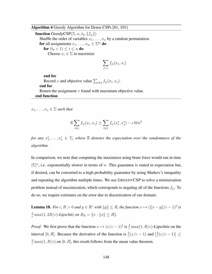
Algorithm 4 Greedy Algorithm for Dense CSPs [81, 101]

function GreedyCSP(Σ, 𝑛, 𝑡0, 𝑓𝑖𝑗)Shuffle the order of variables 𝑥1, . . . , 𝑥𝑛 by a random permutation.for all assignments 𝑥1, . . . , 𝑥𝑡0 ∈ Σ𝑡0 do

for (𝑡0 + 1) ≤ 𝑖 ≤ 𝑛 doChoose 𝑥𝑖 ∈ Σ to maximize ∑

𝑗<𝑖

𝑓𝑗𝑖(𝑥𝑗, 𝑥𝑖)

end forRecord 𝑥 and objective value

∑𝑖 =𝑗 𝑓𝑖𝑗(𝑥𝑖, 𝑥𝑗).

end forReturn the assignment 𝑥 found with maximum objective value.

end function

𝑥1, . . . , 𝑥𝑛 ∈ Σ such that

E∑𝑖 =𝑗

𝑓𝑖𝑗(𝑥𝑖, 𝑥𝑗) ≥∑𝑖 =𝑗

𝑓𝑖𝑗(𝑥*𝑖 , 𝑥

*𝑗)− 𝜖𝑀𝑛2

for any 𝑥*1, . . . , 𝑥

*𝑛 ∈ Σ, where E denotes the expectation over the randomness of the

algorithm.

In comparison, we note that computing the maximizer using brute force would run in time

|Σ|𝑛, i.e. exponentially slower in terms of 𝑛. This guarantee is stated in expectation but,

if desired, can be converted to a high probability guarantee by using Markov’s inequality

and repeating the algorithm multiple times. We use GREEDYCSP to solve a minimization

problem instead of maximization, which corresponds to negating all of the functions 𝑓𝑖𝑗 . To

do so, we require estimates on the error due to discretization of our domain.

Lemma 18. For 𝑐, 𝑅 > 0 and 𝑦 ∈ R𝑟 with ‖𝑦‖ ≤ 𝑅, the function 𝑥 ↦→ (‖𝑥− 𝑦‖/𝑐− 1)2 is2𝑐

max(1, 2𝑅/𝑐)-Lipschitz on 𝐵𝑅 = 𝑥 : ‖𝑥‖ ≤ 𝑅.

Proof. We first prove that the function 𝑥 ↦→ (𝑥/𝑐− 1)2 is 2𝑐

max(1, 𝑅/𝑐)-Lipschitz on the

interval [0, 𝑅]. Because the derivative of the function is 2𝑐(𝑥/𝑐 − 1) and

2𝑐(𝑥/𝑐− 1)

≤

2𝑐

max(1, 𝑅/𝑐) on [0, 𝑅], this result follows from the mean value theorem.

148

Algorithm 5 Approximation Algorithm KKSCHEME

function KKSCHEME(𝜖1, 𝜖2, 𝑅):Build an 𝜖1-net 𝑆𝜖1 of 𝐵𝑅 = 𝑥 : ‖𝑥‖ ≤ 𝑅 ⊂ R𝑟 as in Lemma 12.Apply the GREEDYCSP algorithm of Theorem 18 with 𝜖 = 𝜖2 to approximatelyminimize 𝐸(1, . . . , 𝑛) over 1, . . . , 𝑛 ∈ 𝑆𝑛

𝜖1.

Return 1, . . . , 𝑛.end function

Because the function ‖𝑥 − 𝑦‖ is 1-Lipschitz and ‖𝑥 − 𝑦‖ ≤ ‖𝑥‖ + ‖𝑦‖ ≤ 2𝑅 by the

triangle inequality, the result follows from the fact that 𝑥 ↦→ (𝑥/𝑐− 1)2 is 2𝑐

max(1, 𝑅/𝑐)-

Lipschitz and a composition of Lipschitz functions is Lipschitz.

Combining this result with Lemma 12 we can bound the loss in objective value due to

restricting to a well-chosen discretization.

Lemma 19. Let 1, . . . , 𝑛 ∈ R𝑟 be arbitrary vectors such that ‖𝑖‖ ≤ 𝑅 for all 𝑖 and

𝜖 > 0 be arbitrary. Define 𝑆𝜖 to be an 𝜖-net of 𝐵𝑅 as in Lemma 12, so |𝑆𝜖| ≤ (3𝑅/𝜖)𝑟. For

any input metric over [𝑛] with min𝑖,𝑗∈[𝑛] 𝑑(𝑖, 𝑗) = 1, there exists ′1, . . . ,

′𝑛 ∈ 𝑆𝜖 such that

𝐸(′1, . . . ,

′𝑛) ≤ 𝐸(1, . . . , 𝑛) + 4𝜖𝑅𝑛2

where 𝐸 is (4.5) defined with respect to an arbitrary graph with 𝑛 vertices.

Proof. By Lemma 18 the energy 𝐸(1, . . . , 𝑛) is the sum of(𝑛2

)≤ 𝑛2/2 many terms,

which, for each 𝑖 and 𝑗, are individually 4𝑅-Lipschitz in 𝑖 and 𝑗 . Therefore, defining ′𝑖

to be the closest point in 𝑆𝜖 for all 𝑖 gives the desired result.

This result motivates a straightforward algorithm for producing nearly-optimal layouts

of a graph. Given some graph, by Lemma 15, a sufficiently large radius can be chosen so

that there exists an optimal layout in a ball of that radius. By constructing an 𝜖-net of that

ball, and applying the GREEDYCSP algorithm to the resulting discretization, we obtain a

nearly-optimal layout with theoretical guarantees. This technique is formally described in

the algorithm KKSCHEME. We are now prepared to prove Theorem 17.

149

By combining Lemma 19 with Theorem 18 (used as a minimization instead of maxi-

mization algorithm), the output 1, . . . , 𝑛 of KKSCHEME satisfies

𝐸(1, . . . , 𝑛) ≤ 𝐸(*1, . . . ,

*𝑛) + 4𝜖1𝑅𝑛2 + 𝜖2𝑅

2𝑛2

and runs in time 𝑛22𝑂(1/𝜖22)𝑟 log(3𝑅/𝜖1). Taking 𝜖2 = 𝑂(𝜖/𝑅2) and 𝜖1 = 𝑂(𝜖/𝑅) completes

the proof of Theorem 17.

The runtime can be improved to 𝑛2 + (𝑅/𝜖)𝑂(𝑑𝑅4/𝜖2) using a slightly more complex

greedy CSP algorithm [81]. Also, by the usual argument, a high probability guarantee can

be derived by repeating the algorithm 𝑂(log(2/𝛿)) times, where 𝛿 > 0 is the desired failure

probability.

150

Chapter 5

Error Estimates for the Lanczos Method

5.1 Introduction

The computation of extremal eigenvalues of matrices is one of the most fundamental

problems in numerical linear algebra. When a matrix is large and sparse, methods such

as the Jacobi eigenvalue algorithm and QR algorithm become computationally infeasible,

and, therefore, techniques that take advantage of the sparsity of the matrix are required.

Krylov subspace methods are a powerful class of techniques for approximating extremal

eigenvalues, most notably the Arnoldi iteration for non-symmetric matrices and the Lanczos

method for symmetric matrices.

The Lanczos method is a technique that, given a symmetric matrix 𝐴 ∈ R𝑛×𝑛 and an

initial vector 𝑏 ∈ R𝑛, iteratively computes a tridiagonal matrix 𝑇𝑚 ∈ R𝑚×𝑚 that satisfies

𝑇𝑚 = 𝑄𝑇𝑚𝐴𝑄𝑚, where 𝑄𝑚 ∈ R𝑛×𝑚 is an orthonormal basis for the Krylov subspace

𝒦𝑚(𝐴, 𝑏) = span𝑏, 𝐴𝑏, ..., 𝐴𝑚−1𝑏.

The eigenvalues of 𝑇𝑚, denoted by 𝜆(𝑚)1 (𝐴, 𝑏) ≥ ... ≥ 𝜆

(𝑚)𝑚 (𝐴, 𝑏), are the Rayleigh-Ritz

approximations to the eigenvalues 𝜆1(𝐴) ≥ ... ≥ 𝜆𝑛(𝐴) of 𝐴 on 𝒦𝑚(𝐴, 𝑏), and, therefore,

151

are given by

𝜆(𝑚)𝑖 (𝐴, 𝑏) = min

𝑈⊂𝒦𝑚(𝐴,𝑏)dim(𝑈)=𝑚+1−𝑖

max𝑥∈𝑈𝑥 =0

𝑥𝑇𝐴𝑥

𝑥𝑇𝑥, 𝑖 = 1, ...,𝑚, (5.1)

or, equivalently,

𝜆(𝑚)𝑖 (𝐴, 𝑏) = max

𝑈⊂𝒦𝑚(𝐴,𝑏)dim(𝑈)=𝑖

min𝑥∈𝑈𝑥 =0

𝑥𝑇𝐴𝑥

𝑥𝑇𝑥, 𝑖 = 1, ...,𝑚. (5.2)

This description of the Lanczos method is sufficient for a theoretical analysis of error

(i.e., without round-off error), but, for completeness, we provide a short description of the

Lanczos method (when 𝒦𝑚(𝐴, 𝑏) is full-rank) in Algorithm 6 [113]. For a more detailed

discussion of the nuances of practical implementation and techniques to minimize the effects

of round-off error, we refer the reader to [47, Section 10.3]. If 𝐴 has 𝜈𝑛 non-zero entries,

then Algorithm 6 outputs 𝑇𝑚 after approximately (2𝜈 + 8)𝑚𝑛 floating point operations.

A number of different techniques, such as the divide-and-conquer algorithm with the fast

multipole method [23], can easily compute the eigenvalues of a tridiagonal matrix. The

complexity of this computation is negligible compared to the Lanczos algorithm, as, in

practice, 𝑚 is typically orders of magnitude less than 𝑛.

Equation (5.1) for the Ritz values 𝜆(𝑚)𝑖 illustrates the significant improvement that the

Lanczos method provides over the power method for extremal eigenvalues. Whereas the

power method uses only the iterate 𝐴𝑚𝑏 as an approximation of an eigenvector associated

with the largest magnitude eigenvalue, the Lanczos method uses the span of all of the iterates

of the power method (given by𝒦𝑚+1(𝐴, 𝑏)). However, the analysis of the Lanczos method is

significantly more complicated than that of the power method. Error estimates for extremal

eigenvalue approximation using the Lanczos method have been well studied, most notably

by Kaniel [56], Paige [91], Saad [99], and Kuczynski and Wozniakowski [67] (other notable

work includes [30, 36, 68, 84, 92, 104, 105, 125]). The work of Kaniel, Paige, and Saad

focused on the convergence of the Lanczos method as 𝑚 increases, and, therefore, their

results have strong dependence on the spectrum of the matrix 𝐴 and the choice of initial

152

vector 𝑏. For example, a standard result of this type is the estimate

𝜆1(𝐴)− 𝜆(𝑚)1 (𝐴, 𝑏)

𝜆1(𝐴)− 𝜆𝑛(𝐴)≤(

tan∠(𝑏, 𝜙1)

𝑇𝑚−1(1 + 2𝛾)

)2

, 𝛾 =𝜆1(𝐴)− 𝜆2(𝐴)

𝜆2(𝐴)− 𝜆𝑛(𝐴), (5.3)

where 𝜙1 is the eigenvector corresponding to 𝜆1, and 𝑇𝑚−1 is the (𝑚−1)𝑡ℎ degree Chebyshev

polynomial of the first kind [100, Theorem 6.4]. Kuczynski and Wozniakowski took a quite

different approach, and estimated the maximum expected relative error (𝜆1 − 𝜆(𝑚)1 )/𝜆1 over

all 𝑛× 𝑛 symmetric positive definite matrices, resulting in error estimates that depend only

on the dimension 𝑛 and the number of iterations 𝑚. They produced the estimate

sup𝐴∈𝒮𝑛

++

E𝑏∼𝒰(𝑆𝑛−1)

[𝜆1(𝐴)− 𝜆

(𝑚)1 (𝐴, 𝑏)

𝜆1(𝐴)

]≤ .103

ln2(𝑛(𝑚− 1)4)

(𝑚− 1)2, (5.4)

for all 𝑛 ≥ 8 and 𝑚 ≥ 4, where 𝒮𝑛++ is the set of all 𝑛 × 𝑛 symmetric positive definite

matrices, and the expectation is with respect to the uniform probability measure on the

hypersphere 𝑆𝑛−1 = 𝑥 ∈ R𝑛 | ‖𝑥‖ = 1 [67, Theorem 3.2]. One can quickly verify

that equation (5.4) also holds when the 𝜆1(𝐴) term in the denominator is replaced by

𝜆1(𝐴)− 𝜆𝑛(𝐴), and the supremum over 𝒮𝑛++ is replaced by the maximum over the set of all

𝑛× 𝑛 symmetric matrices, denoted by 𝒮𝑛.

Both of these approaches have benefits and drawbacks. If an extremal eigenvalue is

known to have a reasonably large eigenvalue gap (based on application or construction),

then a distribution dependent estimate provides a very good approximation of error, even for

small 𝑚. However, if the eigenvalue gap is not especially large, then distribution dependent

estimates can significantly overestimate error, and estimates that depend only on 𝑛 and 𝑚

are preferable. This is illustrated by the following elementary, yet enlightening, example.

Example 1. Let 𝐴 ∈ 𝑆𝑛++ be the tridiagonal matrix resulting from the discretization of the

Laplacian operator on an interval with Dirichlet boundary conditions, namely, 𝐴𝑖,𝑖 = 2

for 𝑖 = 1, ..., 𝑛 and 𝐴𝑖,𝑖+1 = 𝐴𝑖+1,𝑖 = −1 for 𝑖 = 1, ..., 𝑛 − 1. The eigenvalues of 𝐴

are given by 𝜆𝑖(𝐴) = 2 + 2 cos (𝑖𝜋/(𝑛 + 1)), 𝑖 = 1, ..., 𝑛. Consider the approximation

of 𝜆1(𝐴) by 𝑚 iterations of the Lanczos method. For a random choice of 𝑏, the expected

153

Algorithm 6 Lanczos Method

Input: symmetric matrix 𝐴 ∈ R𝑛×𝑛, vector 𝑏 ∈ R𝑛, number of iterations 𝑚.

Output: symmetric tridiagonal matrix 𝑇𝑚 ∈ R𝑚×𝑚, 𝑇𝑚(𝑖, 𝑖) = 𝛼𝑖,

𝑇𝑚(𝑖, 𝑖 + 1) = 𝛽𝑖, satisfying 𝑇𝑚 = 𝑄𝑇𝑚𝐴𝑄𝑚, where 𝑄𝑚 = [𝑞1 ... 𝑞𝑚].

Set 𝛽0 = 0, 𝑞0 = 0, 𝑞1 = 𝑏/‖𝑏‖

For 𝑖 = 1, ...,𝑚

𝑣 = 𝐴𝑞𝑖

𝛼𝑖 = 𝑞𝑇𝑖 𝑣

𝑣 = 𝑣 − 𝛼𝑖𝑞𝑖 − 𝛽𝑖−1𝑞𝑖−1

𝛽𝑖 = ‖𝑣‖𝑞𝑖+1 = 𝑣/𝛽𝑖

value of tan2∠(𝑏, 𝜙1) is (1+𝑜(1))𝑛. If tan2∠(𝑏, 𝜙1) = 𝐶𝑛 for some constant 𝐶, then (5.3)

produces the estimate

𝜆1(𝐴)− 𝜆(𝑚)1 (𝐴, 𝑏)

𝜆1(𝐴)− 𝜆𝑛(𝐴)≤ 𝐶𝑛𝑇𝑚−1

(1 + 2 tan

(𝜋

2(𝑛 + 1)

)tan

(3𝜋

2(𝑛 + 1)

))−2

≃ 𝑛(1 + 𝑂(𝑛−1))−𝑚 ≃ 𝑛.

In this instance, the estimate is a trivial one for all choices of 𝑚, which varies greatly from

the error estimate (5.4) of order ln2 𝑛/𝑚2. The exact same estimate holds for the smallest

eigenvalue 𝜆𝑛(𝐴) when the corresponding bounds are applied, since 4𝐼 −𝐴 is similar to 𝐴.

Now, consider the approximation of the largest eigenvalue of 𝐵 = 𝐴−1 by 𝑚 iterations

of the Lanczos method. The matrix 𝐵 possesses a large gap between the largest and second-

largest eigenvalue, which results in a value of 𝛾 for (5.3) that remains bounded below by a

constant independent of 𝑛, namely

𝛾 = (2 cos (𝜋/(𝑛 + 1)) + 1) / (2 cos (𝜋/(𝑛 + 1))− 1) .

154

Therefore, in this instance, the estimate (5.3) illustrates a constant convergence rate, pro-

duces non-trivial bounds (for typical 𝑏) for 𝑚 = Θ(ln𝑛), and is preferable to the error

estimate (5.4) of order ln2 𝑛/𝑚2.

More generally, if a matrix 𝐴 has eigenvalue gap 𝛾 . 𝑛−𝛼 and the initial vector 𝑏

satisfies tan2∠(𝑏, 𝜙1) & 𝑛, then the error estimate (5.3) is a trivial one for 𝑚 . 𝑛𝛼/2. This

implies that the estimate (5.3) is most useful when the eigenvalue gap is constant or tends to

zero very slowly as 𝑛 increases. When the gap is not especially large (say, 𝑛−𝛼, 𝛼 constant),

then uniform error estimates are preferable for small values of 𝑚. In this work, we focus

on uniform bounds, namely, error estimates that hold uniformly over some large set of

matrices (typically 𝒮𝑛++ or 𝒮𝑛). We begin by recalling some of the key existing uniform

error estimates for the Lanczos method.

5.1.1 Related Work

Uniform error estimates for the Lanczos method have been produced almost exclusively

for symmetric positive definite matrices, as error estimates for extremal eigenvalues of

symmetric matrices can be produced from estimates for 𝑆𝑛++ relatively easily. The majority

of results apply only to either 𝜆1(𝐴), 𝜆𝑛(𝐴), or some function of the two (i.e., condition

number). All estimates are probabilistic and take the initial vector 𝑏 to be uniformly

distributed on the hypersphere. Here we provide a brief description of some key uniform

error estimates previously produced for the Lanczos method.

In [67], Kuczynski and Wozniakowski produced a complete analysis of the power

method and provided a number of upper bounds for the Lanczos method. Most notably, they

produced error estimate (5.4) and provided the following upper bound for the probability

that the relative error (𝜆1 − 𝜆(𝑚)1 )/𝜆1 is greater than some value 𝜖:

sup𝐴∈𝒮𝑛

++

P𝑏∼𝒰(𝑆𝑛−1)

[𝜆1(𝐴)− 𝜆

(𝑚)1 (𝐴, 𝑏)

𝜆1(𝐴)> 𝜖

]≤ 1.648

√𝑛𝑒−

√𝜖(2𝑚−1). (5.5)

However, the authors were unable to produce any lower bounds for (5.4) or (5.5), and stated

that a more sophisticated analysis would most likely be required. In the same paper, they

155

performed numerical experiments for the Lanczos method that produced errors of the order

𝑚−2, which led the authors to suggest that the error estimate (5.4) may be an overestimate,

and that the ln2 𝑛 term may be unnecessary.

In [68], Kuczynski and Wozniakowski noted that the above estimates immediately

translate to relative error estimates for minimal eigenvalues when the error 𝜆(𝑚)𝑚 − 𝜆𝑛 is

considered relative to 𝜆1 or 𝜆1 − 𝜆𝑛 (both normalizations can be shown to produce the

same bound). However, we can quickly verify that there exist sequences in 𝒮𝑛++ for which

the quantity E[(𝜆

(𝑚)𝑚 − 𝜆𝑛)/𝜆𝑛

]is unbounded. These results for minimal eigenvalues,

combined with (5.4), led to error bounds for estimating the condition number of a matrix.

Unfortunately, error estimates for the condition number face the same issue as the quantity

(𝜆(𝑚)𝑚 − 𝜆𝑛)/𝜆𝑛, and therefore, only estimates that depend on the value of the condition

number can be produced.

The proof technique used to produce (5.4) works specifically for the quantity E[(𝜆1 −

𝜆(𝑚)1 )/𝜆1

](i.e., the 1-norm), and does not carry over to more general 𝑝-norms of the form

E[((𝜆1 − 𝜆

(𝑚)1 )/𝜆1)

𝑝]1/𝑝, 𝑝 ∈ (1,∞). Later, in [30, Theorem 5.2, 𝑟 = 1], Del Corso and

Manzini produced an upper bound of the order (√𝑛/𝑚)1/𝑝 for arbitrary 𝑝-norms, given by

sup𝐴∈𝒮𝑛

++

E𝑏∼𝒰(𝑆𝑛−1)

[(𝜆1(𝐴)− 𝜆

(𝑚)1 (𝐴, 𝑏)

𝜆1(𝐴)

)𝑝] 1𝑝

.1

𝑚1/𝑝

(Γ(𝑝− 1

2

)Γ(𝑛2

)Γ(𝑝)Γ

(𝑛−12

) ) 1𝑝

. (5.6)

This bound is clearly worse than (5.4), and better bounds can be produced for arbitrary 𝑝

simply by making use of (5.5). Again, the authors were unable to produce any lower bounds.

More recently, the machine learning and optimization community has become increas-

ingly interested in the problem of approximating the top singular vectors of a symmetric

matrix by randomized techniques (for a review, see [49]). This has led to a wealth of new

results in recent years regarding classical techniques, including the Lanczos method. In

[84], Musco and Musco considered a block Krylov subspace algorithm similar to the block

Lanczos method and showed that with high probability their algorithm achieves an error of

𝜖 in 𝑚 = 𝑂(𝜖−1/2 ln𝑛) iterations, matching the bound (5.5) for a block size of one. Very

recently, a number of lower bounds for a wide class of randomized algorithms were shown

156

in [104, 105], all of which can be applied to the Lanczos method as a corollary. First, the

authors showed that the dependence on 𝑛 in the above upper bounds was in fact necessary.

In particular, it follows from [105, Theorem A.1] that 𝑂(log 𝑛) iterations are necessary to

obtain a non-trivial error. In addition, as a corollary of their main theorem [105, Theorem

1], there exist 𝑐1, 𝑐2 > 0 such that for all 𝜖 ∈ (0, 1) there exists an 𝑛𝑜 = poly(𝜖−1) such that

for all 𝑛 ≥ 𝑛𝑜 there exists a random matrix 𝐴 ∈ 𝒮𝑛 such that

P[𝜌(𝐴)− 𝜌(𝑇 )

𝜌(𝐴)≥ 𝜖

12

]≥ 1− 𝑒−𝑛𝑐2 for all 𝑚 ≤ 𝑐1𝜖

−1/2 ln𝑛, (5.7)

where 𝜌(·) is the spectral radius of a matrix, and the randomness is over both the initial

vector and matrix.

5.1.2 Contributions and Remainder of Chapter

In what follows, we prove improved upper bounds for the maximum expected error of the

Lanczos method in the 𝑝-norm, 𝑝 ≥ 1, and combine this with nearly-matching asymptotic

lower bounds with explicit constants. These estimates can be found in Theorem 19. The

upper bounds result from using a slightly different proof technique than that of (5.4), which

is more robust to arbitrary 𝑝-norms. Comparing the lower bounds of Theorem 19 to the

estimate (5.7), we make a number of observations. Whereas (5.7) results from a statistical

analysis of random matrices, our estimates follow from taking an infinite sequence of non-

random matrices with explicit eigenvalues and using the theory of orthogonal polynomials.

Our estimate for 𝑚 = 𝑂(ln𝑛) (in Theorem 19) is slightly worse than (5.7) by a factor

of ln2 ln𝑛, but makes up for this in the form of an explicit constant. The estimate for

𝑚 = 𝑜(𝑛1/2 ln−1/2 𝑛) (also in Theorem 19) does not have 𝑛 dependence, but illustrates a

useful lower bound, as it has an explicit constant and the ln𝑛 term becomes negligible as

𝑚 increases. The results (5.7) do not fully apply to this regime, as the dependence of the

required lower bound on 𝑛 is at least cubic in the inverse of the eigenvalue gap (see [105,

Theorem 6.1] for details).

To complement these bounds, we also provide an error analysis for matrices that have a

157

certain structure. In Theorem 20, we produce improved dimension-free upper bounds for

matrices that have some level of eigenvalue “regularity" near 𝜆1. In addition, in Theorem 21,

we prove a powerful result that can be used to determine, for any fixed 𝑚, the asymptotic

relative error for any sequence of matrices 𝑋𝑛 ∈ 𝒮𝑛, 𝑛 = 1, 2, ..., that exhibits suitable

convergence of its empirical spectral distribution. Later, we perform numerical experiments

that illustrate the practical usefulness of this result. Theorem 21, combined with estimates

for Jacobi polynomials (see Proposition 13), illustrates that the inverse quadratic dependence

on the number of iterations 𝑚 in the estimates produced throughout this chapter does not

simply illustrate the worst case, but is actually indicative of the typical case in some sense.

In Corollary 3 and Theorem 22, we produce results similar to Theorem 19 for arbitrary

eigenvalues 𝜆𝑖. The lower bounds follow relatively quickly from the estimates for 𝜆1, but

the upper bounds require some mild assumptions on the eigenvalue gaps of the matrix.

These results mark the first uniform-type bounds for estimating arbitrary eigenvalues by

the Lanczos method. In addition, in Corollary 4, we translate our error estimates for the

extremal eigenvalues 𝜆1(𝐴) and 𝜆𝑛(𝐴) into error bounds for the condition number of a

symmetric positive definite matrix, but, as previously mentioned, the relative error of the

condition number of a matrix requires estimates that depend on the condition number itself.

Finally, we present numerical experiments that support the accuracy and practical usefulness

of the theoretical estimates detailed above.

The remainder of the chapter is as follows. In Section 5.2, we prove basic results

regarding relative error and make a number of fairly straightforward observations. In Section

5.3, we prove asymptotic lower bounds and improved upper bounds for the relative error

in an arbitrary 𝑝-norm. In Section 5.4, we produce a dimension-free error estimate for a

large class of matrices and prove a theorem that can be used to determine the asymptotic

relative error for any fixed 𝑚 and sequence of matrices 𝑋𝑛 ∈ 𝒮𝑛, 𝑛 = 1, 2, ..., with suitable

convergence of its empirical spectral distribution. In Section 5.5, under some mild additional

assumptions, we prove a version of Theorem 19 for arbitrary eigenvalues 𝜆𝑖, and extend

our results for 𝜆1 and 𝜆𝑛 to the condition number of a symmetric positive definite matrix.

Finally, in Section 5.6, we perform a number of experiments and discuss how the numerical

158

results compare to the theoretical estimates in this work.

5.2 Preliminary Results

Because the Lanczos method applies only to symmetric matrices, all matrices in this

chapter are assumed to belong to 𝒮𝑛. The Lanczos method and the quantity (𝜆1(𝐴) −

𝜆(𝑚)1 (𝐴, 𝑏))/(𝜆1(𝐴) − 𝜆𝑛(𝐴)) are both unaffected by shifting and scaling, and so any

maximum over 𝐴 ∈ 𝒮𝑛 can be replaced by a maximum over all 𝐴 ∈ 𝒮𝑛 with 𝜆1(𝐴) and

𝜆𝑛(𝐴) fixed. Often for producing upper bounds, it is convenient to choose 𝜆1(𝐴) = 1 and

𝜆𝑛(𝐴) = 0. For the sake of brevity, we will often write 𝜆𝑖(𝐴) and 𝜆(𝑚)𝑗 (𝐴, 𝑏) as 𝜆𝑖 and 𝜆

(𝑚)𝑗

when the associated matrix 𝐴 and vector 𝑏 are clear from context.

We begin by rewriting expression (5.2) for 𝜆(𝑚)1 in terms of polynomials. The Krylov

subspace 𝒦𝑚(𝐴, 𝑏) can be alternatively defined as

𝒦𝑚(𝐴, 𝑏) = 𝑃 (𝐴)𝑏 |𝑃 ∈ 𝒫𝑚−1,

where 𝒫𝑚−1 is the set of all real-valued polynomials of degree at most 𝑚 − 1. Suppose

𝐴 ∈ 𝒮𝑛 has eigendecomposition 𝐴 = 𝑄Λ𝑄𝑇 , where 𝑄 ∈ R𝑛×𝑛 is an orthogonal matrix and

Λ ∈ R𝑛×𝑛 is the diagonal matrix satisfying Λ(𝑖, 𝑖) = 𝜆𝑖(𝐴), 𝑖 = 1, ..., 𝑛. Then we have the

relation

𝜆(𝑚)1 (𝐴, 𝑏) = max

𝑥∈𝒦𝑚(𝐴,𝑏)𝑥 =0

𝑥𝑇𝐴𝑥

𝑥𝑇𝑥= max

𝑃∈𝒫𝑚−1𝑃 =0

𝑏𝑇𝑃 2(𝐴)𝐴𝑏

𝑏𝑇𝑃 2(𝐴)𝑏= max

𝑃∈𝒫𝑚−1𝑃 =0

𝑇𝑃 2(Λ)Λ

𝑇𝑃 2(Λ),

where = 𝑄𝑇 𝑏. The relative error is given by

𝜆1(𝐴)− 𝜆(𝑚)1 (𝐴, 𝑏)

𝜆1(𝐴)− 𝜆𝑛(𝐴)= min

𝑃∈𝒫𝑚−1𝑃 =0

∑𝑛𝑖=2

2𝑖𝑃

2(𝜆𝑖)(𝜆1 − 𝜆𝑖)

(𝜆1 − 𝜆𝑛)∑𝑛

𝑖=1 2𝑖𝑃

2(𝜆𝑖),

159

and the expected 𝑝𝑡ℎ moment of the relative error is given by

E𝑏∼𝒰(𝑆𝑛−1)

[(𝜆1 − 𝜆

(𝑚)1

𝜆1 − 𝜆𝑛

)𝑝]=

∫𝑆𝑛−1

min𝑃∈𝒫𝑚−1

𝑃 =0

[ ∑𝑛𝑖=2

2𝑖𝑃

2(𝜆𝑖)(𝜆1 − 𝜆𝑖)

(𝜆1 − 𝜆𝑛)∑𝑛

𝑖=1 2𝑖𝑃

2(𝜆𝑖)

]𝑝𝑑𝜎(),

where 𝜎 is the uniform probability measure on 𝑆𝑛−1. Because the relative error does not

depend on the norm of or the sign of any entry, we can replace the integral over 𝑆𝑛−1 by

an integral of 𝑦 = (𝑦1, ..., 𝑦𝑛) over [0,∞)𝑛 with respect to the joint chi-square probability

density function

𝑓𝑌 (𝑦) =1

(2𝜋)𝑛/2exp

−1

2

𝑛∑𝑖=1

𝑦𝑖

𝑛∏

𝑖=1

𝑦−12

𝑖 (5.8)

of 𝑛 independent chi-square random variables 𝑌1, ..., 𝑌𝑛 ∼ 𝜒21 with one degree of freedom

each. In particular, we have

E𝑏∼𝒰(𝑆𝑛−1)

[(𝜆1 − 𝜆

(𝑚)1

𝜆1 − 𝜆𝑛

)𝑝]=

∫[0,∞)𝑛

min𝑃∈𝒫𝑚−1

𝑃 =0

[ ∑𝑛𝑖=2 𝑦𝑖𝑃

2(𝜆𝑖)(𝜆1 − 𝜆𝑖)

(𝜆1 − 𝜆𝑛)∑𝑛

𝑖=1 𝑦𝑖𝑃2(𝜆𝑖)

]𝑝𝑓𝑌 (𝑦) 𝑑𝑦.

(5.9)

Similarly, probabilistic estimates with respect to 𝑏 ∼ 𝒰(𝑆𝑛−1) can be replaced by estimates

with respect to 𝑌1, ..., 𝑌𝑛 ∼ 𝜒21, as

P𝑏∼𝒰(𝑆𝑛−1)

[𝜆1 − 𝜆

(𝑚)1

𝜆1 − 𝜆𝑛

≥ 𝜖

]= P

𝑌𝑖∼𝜒21

⎡⎣ min𝑃∈𝒫𝑚−1

𝑃 =0

∑𝑛𝑖=2 𝑌𝑖𝑃

2(𝜆𝑖)(𝜆1 − 𝜆𝑖)

(𝜆1 − 𝜆𝑛)∑𝑛

𝑖=1 𝑌𝑖𝑃 2(𝜆𝑖)≥ 𝜖

⎤⎦ . (5.10)

For the remainder of the chapter, we almost exclusively use equation (5.9) for expected

relative error and equation (5.10) for probabilistic bounds for relative error. If 𝑃 minimizes

the expression in equation (5.9) or (5.10) for a given 𝑦 or 𝑌 , then any polynomial of the

form 𝛼𝑃 , 𝛼 ∈ R∖0, is also a minimizer. Therefore, without any loss of generality, we

can alternatively minimize over the set 𝒫𝑚−1(1) = 𝑄 ∈ 𝒫𝑚−1 |𝑄(1) = 1. For the sake

of brevity, we will omit the subscripts under E and P when the underlying distribution

is clear from context. In this work, we make use of asymptotic notation to express the

limiting behavior of a function with respect to 𝑛. A function 𝑓(𝑛) is 𝑂(𝑔(𝑛)) if there exists

𝑀,𝑛0 > 0 such that |𝑓(𝑛)| ≤𝑀𝑔(𝑛) for all 𝑛 ≥ 𝑛0, 𝑜(𝑔(𝑛)) if for every 𝜖 > 0 there exists

160

a 𝑛𝜖 such that |𝑓(𝑛)| ≤ 𝜖𝑔(𝑛) for all 𝑛 ≥ 𝑛0, 𝜔(𝑔(𝑛)) if |𝑔(𝑛)| = 𝑜(|𝑓(𝑛)|), and Θ(𝑔(𝑛)) if

𝑓(𝑛) = 𝑂(𝑔(𝑛)) and 𝑔(𝑛) = 𝑂(𝑓(𝑛)).

5.3 Asymptotic Lower Bounds and Improved Upper Bounds

In this section, we obtain improved upper bounds for E[((𝜆1 − 𝜆

(𝑚)1 )/𝜆1)

𝑝]1/𝑝, 𝑝 ≥ 1, and

produce nearly-matching lower bounds. In particular, we prove the following theorem for

the behavior of 𝑚 as a function of 𝑛 as 𝑛 tends to infinity.

Theorem 19.

max𝐴∈𝒮𝑛

P𝑏∼𝒰(𝑆𝑛−1)

[𝜆1(𝐴)− 𝜆

(𝑚)1 (𝐴, 𝑏)

𝜆1(𝐴)− 𝜆𝑛(𝐴)≥ 1− 𝑜(1)

]≥ 1− 𝑜(1/𝑛)

for 𝑚 = 𝑜(ln𝑛),

max𝐴∈𝒮𝑛

P𝑏∼𝒰(𝑆𝑛−1)

[𝜆1(𝐴)− 𝜆

(𝑚)1 (𝐴, 𝑏)

𝜆1(𝐴)− 𝜆𝑛(𝐴)≥ .015 ln2 𝑛

𝑚2 ln2 ln𝑛

]≥ 1− 𝑜(1/𝑛)

for 𝑚 = Θ(ln𝑛),

max𝐴∈𝒮𝑛

P𝑏∼𝒰(𝑆𝑛−1)

[𝜆1(𝐴)− 𝜆

(𝑚)1 (𝐴, 𝑏)

𝜆1(𝐴)− 𝜆𝑛(𝐴)≥ 1.08

𝑚2

]≥ 1− 𝑜(1/𝑛)

for 𝑚 = 𝑜(𝑛1/2 ln−1/2 𝑛

)and 𝜔(1), and

max𝐴∈𝒮𝑛

E𝑏∼𝒰(𝑆𝑛−1)

[(𝜆1(𝐴)− 𝜆

(𝑚)1 (𝐴, 𝑏)

𝜆1(𝐴)− 𝜆𝑛(𝐴)

)𝑝]1/𝑝≤ .068

ln2 (𝑛(𝑚− 1)8𝑝)

(𝑚− 1)2

for 𝑛 ≥ 100, 𝑚 ≥ 10, 𝑝 ≥ 1.

Proof. The first result is a corollary of [105, Theorem A.1], and the remaining results follow

from Lemmas 20, 21, and 22.

By Hölder’s inequality, the lower bounds in Theorem 19 also hold for arbitrary 𝑝-norms,

161

𝑝 ≥ 1. All results are equally applicable to 𝜆𝑛, as the Krylov subspace is unaffected by

shifting and scaling, namely 𝒦𝑚(𝐴, 𝑏) = 𝒦𝑚(𝛼𝐴 + 𝛽𝐼, 𝑏) for all 𝛼 = 0.

We begin by producing asymptotic lower bounds. The general technique is as follows.

We choose an infinite sequence of matrices 𝐴𝑛∞𝑛=1, 𝐴𝑛 ∈ 𝒮𝑛, treat 𝑚 as a function of 𝑛,

and show that, as 𝑛 tends to infinity, for “most" choices of an initial vector 𝑏, the relative error

of this sequence of matrices is well approximated by an integral polynomial minimization

problem for which bounds can be obtained. First, we recall a number of useful propositions

regarding Gauss-Legendre quadrature, orthogonal polynomials, and Chernoff bounds for

chi-square random variables.

Proposition 9. ([41],[114]) Let 𝑃 ∈ 𝒫2𝑘−1, 𝑥𝑖𝑘𝑖=1 be the zeros of the 𝑘𝑡ℎ degree Legendre

polynomial 𝑃𝑘(𝑥), 𝑃𝑘(1) = 1, in descending order (𝑥1 > ... > 𝑥𝑘), and 𝑤𝑖 = 2(1 −

𝑥2𝑖 )

−1[𝑃 ′𝑘(𝑥𝑖)]

−2, 𝑖 = 1, ..., 𝑘 be the corresponding weights. Then

1.∫ 1

−1

𝑃 (𝑥) 𝑑𝑥 =𝑘∑

𝑖=1

𝑤𝑖𝑃 (𝑥𝑖),

2. 𝑥𝑖 =(1− 1

8𝑘2

)cos(

(4𝑖−1)𝜋4𝑘+2

)+ 𝑂(𝑘−3), 𝑖 = 1, ..., 𝑘,

3.𝜋

𝑘 + 12

√1− 𝑥2

1

(1− 1

8(𝑘 + 12)2(1− 𝑥2

1)

)≤ 𝑤1 < ... < 𝑤⌊𝑘+1

2

⌋ ≤ 𝜋

𝑘 + 12

.

Proposition 10. ([110, Section 7.72], [111]) Let 𝜔(𝑥) 𝑑𝑥 be a measure on [−1, 1] with

infinitely many points of increase, with orthogonal polynomials 𝑝𝑘(𝑥)𝑘≥0, 𝑝𝑘 ∈ 𝒫𝑘. Then

max𝑃∈𝒫𝑘𝑃 =0

∫ 1

−1𝑥𝑃 2(𝑥)𝜔(𝑥) 𝑑𝑥∫ 1

−1𝑃 2(𝑥)𝜔(𝑥) 𝑑𝑥

= max𝑥 ∈ [−1, 1]

𝑝𝑘+1(𝑥) = 0

.

Proposition 11. Let 𝑍 ∼ 𝜒2𝑘. Then P[𝑍 ≤ 𝑥] ≤

[𝑥𝑘

exp

1− 𝑥𝑘

]𝑘2 for 𝑥 ≤ 𝑘 and

P[𝑍 ≥ 𝑥] ≤[𝑥𝑘

exp

1− 𝑥𝑘

]𝑘2 for 𝑥 ≥ 𝑘.

Proof. The result follows from taking [26, Lemma 2.2] and letting 𝑑→∞.

We are now prepared to prove a lower bound of order 𝑚−2.

162

Lemma 20. If 𝑚 = 𝑜(𝑛1/2 ln−1/2 𝑛

)and 𝜔(1), then

max𝐴∈𝒮𝑛

P𝑏∼𝒰(𝑆𝑛−1)

[𝜆1(𝐴)− 𝜆

(𝑚)1 (𝐴, 𝑏)

𝜆1(𝐴)− 𝜆𝑛(𝐴)≥ 1.08

𝑚2

]≥ 1− 𝑜(1/𝑛).

Proof. The structure of the proof is as follows. We choose a matrix with eigenvalues based

on the zeros of a Legendre polynomial, and show that a large subset of [0,∞)𝑛 (with

respect to 𝑓𝑌 (𝑦)) satisfies conditions that allow us to lower bound the relative error using an

integral minimization problem. The choice of Legendre polynomials is based on connections

to Gaussian quadrature, but, as we will later see (in Theorem 21 and experiments), the

1/𝑚2 dependence is indicative of a large class of matrices with connections to orthogonal

polynomials. Let 𝑥1 > ... > 𝑥2𝑚 be the zeros of the (2𝑚)𝑡ℎ degree Legendre polynomial.

Let 𝐴 ∈ 𝒮𝑛 have eigenvalue 𝑥1 with multiplicity one, and remaining eigenvalues given by

𝑥𝑗 , 𝑗 = 2, ..., 2𝑚, each with multiplicity at least ⌊(𝑛− 1)/(2𝑚− 1)⌋. By equation (5.10),

P

[𝜆1 − 𝜆

(𝑚)1

𝜆1 − 𝜆𝑛

≥ 𝜖

]= P

⎡⎣ min𝑃∈𝒫𝑚−1

𝑃 =0

∑𝑛𝑖=2 𝑌𝑖𝑃

2(𝜆𝑖)(𝜆1 − 𝜆𝑖)

(𝜆1 − 𝜆𝑛)∑𝑛

𝑖=1 𝑌𝑖𝑃 2(𝜆𝑖)≥ 𝜖

⎤⎦= P

⎡⎣ min𝑃∈𝒫𝑚−1

𝑃 =0

∑2𝑚𝑗=2 𝑌𝑗𝑃

2(𝑥𝑗) (𝑥1 − 𝑥𝑗)

(𝑥1 − 𝑥2𝑚)∑2𝑚

𝑗=1 𝑌𝑗𝑃 2 (𝑥𝑗)≥ 𝜖

⎤⎦ ,

where 𝑌1, ..., 𝑌𝑛 ∼ 𝜒21, and 𝑌𝑗 is the sum of the 𝑌𝑖 that satisfy 𝜆𝑖 = 𝑥𝑗 . 𝑌1 has one degree of

freedom, and 𝑌𝑗 , 𝑗 = 2, ..., 2𝑚, each have at least ⌊(𝑛− 1)/(2𝑚− 1)⌋ degrees of freedom.

Let 𝑤1, ..., 𝑤2𝑚 be the weights of Gaussian quadrature associated with 𝑥1, ..., 𝑥2𝑚. By

Proposition 9,

𝑥1 = 1− 4 + 9𝜋2

128𝑚2+ 𝑂(𝑚−3), 𝑥2 = 1− 4 + 49𝜋2

128𝑚2+ 𝑂(𝑚−3),

and, therefore, 1− 𝑥21 = 4+9𝜋2

64𝑚2 + 𝑂(𝑚−3). Again, by Proposition 9, we can lower bound

163

the smallest ratio between weights by

𝑤1

𝑤𝑚

≥√

1− 𝑥21

(1− 1

8(2𝑚 + 1/2)2(1− 𝑥21)

)=

(√4 + 9𝜋2

8𝑚+ 𝑂(𝑚−2)

)(1− 1

(4 + 9𝜋2)/2 + 𝑂(𝑚−1)

)=

2 + 9𝜋2

8√

4 + 9𝜋2𝑚+ 𝑂(𝑚−2).

Therefore, by Proposition 11,

P[min𝑗≥2

𝑌𝑗 ≥𝑤𝑚

𝑤1

𝑌1

]≥ P

[𝑌𝑗 ≥

1

3

⌊𝑛− 1

2𝑚− 1

⌋, 𝑗 ≥ 2

]× P

[𝑌1 ≤

𝑤1

3𝑤𝑚

⌊𝑛− 1

2𝑚− 1

⌋]

≥[1−

(𝑒2/3

3

)12

⌊𝑛−12𝑚−1

⌋ ]2𝑚−1[1−

(𝑤1

3𝑤𝑚

⌊𝑛−12𝑚−1

⌋𝑒1− 𝑤1

3𝑤𝑚

⌊𝑛−12𝑚−1

⌋)12]

= 1− 𝑜(1/𝑛).

We now restrict our attention to values of 𝑌 = (𝑌1, ..., 𝑌𝑛) ∈ [0,∞)𝑛 that satisfy the

inequality 𝑤1 min𝑗≥2 𝑌𝑗 ≥ 𝑤𝑚𝑌1. If, for some fixed choice of 𝑌 ,

min𝑃∈𝒫𝑚−1

𝑃 =0

∑2𝑚𝑗=2 𝑌𝑗𝑃

2(𝑥𝑗)(𝑥1 − 𝑥𝑗)∑2𝑚𝑗=1 𝑌𝑗𝑃 2(𝑥𝑗)

≤ 𝑥1 − 𝑥2, (5.11)

then, by Proposition 9 and Proposition 10 for 𝜔(𝑥) = 1,

min𝑃∈𝒫𝑚−1

𝑃 =0

∑2𝑚𝑗=2 𝑌𝑗𝑃

2(𝑥𝑗)(𝑥1 − 𝑥𝑗)∑2𝑚𝑗=1 𝑌𝑗𝑃 2(𝑥𝑗)

≥ min𝑃∈𝒫𝑚−1

𝑃 =0

∑2𝑚𝑗=2𝑤𝑗𝑃

2(𝑥𝑗)(𝑥1 − 𝑥𝑗)∑2𝑚𝑗=1𝑤𝑗𝑃 2(𝑥𝑗)

= min𝑃∈𝒫𝑚−1

𝑃 =0

∑2𝑚𝑗=1 𝑤𝑗𝑃

2(𝑥𝑗)(1− 𝑥𝑗)∑2𝑚𝑗=1𝑤𝑗𝑃 2(𝑥𝑗)

− (1− 𝑥1)

= min𝑃∈𝒫𝑚−1

𝑃 =0

∫ 1

−1

𝑃 2(𝑦)(1− 𝑦) 𝑑𝑦∫ 1

−1

𝑃 2(𝑦) 𝑑𝑦

− 4 + 9𝜋2

128𝑚2+ 𝑂(𝑚−3)

=4 + 9𝜋2

32𝑚2− 4 + 9𝜋2

128𝑚2+ 𝑂(𝑚−3) =

12 + 27𝜋2

128𝑚2+ 𝑂(𝑚−3).

164

Alternatively, if equation (5.11) does not hold, then we can lower bound the left hand side

of (5.11) by 𝑥1 − 𝑥2 = 5𝜋2

16𝑚2 + 𝑂(𝑚−3). Noting that 𝑥1 − 𝑥2𝑚 ≤ 2 completes the proof, as12+27𝜋2

256and 5𝜋2

32are both greater than 1.08.

The previous lemma illustrates that the inverse quadratic dependence of the relative

error on the number of iterations 𝑚 persists up to 𝑚 = 𝑜(𝑛1/2/ ln1/2 𝑛). As we will see

in Sections 4 and 6, this 𝑚−2 error is indicative of the behavior of the Lanczos method

for a wide range of typical matrices encountered in practice. Next, we aim to produce a

lower bound of the form ln2 𝑛/(𝑚2 ln2 ln𝑛). To do so, we will make use of more general

Jacobi polynomials instead of Legendre polynomials. In addition, in order to obtain a result

that contains some dependence on 𝑛, the choice of Jacobi polynomial must vary with 𝑛

(i.e., 𝛼 and 𝛽 are a function of 𝑛). However, due to the distribution of eigenvalues required

to produce this bound, Gaussian quadrature is no longer exact, and we must make use of

estimates for basic composite quadrature. We recall the following propositions regarding

composite quadrature and Jacobi polynomials.

Proposition 12. If 𝑓 ∈ 𝒞1[𝑎, 𝑏], then for 𝑎 = 𝑥0 < ... < 𝑥𝑛 = 𝑏,∫ 𝑏

𝑎

𝑓(𝑥) 𝑑𝑥−𝑛∑

𝑖=1

(𝑥𝑖 − 𝑥𝑖−1)𝑓(𝑥*𝑖 )

≤ 𝑏− 𝑎

2max𝑥∈[𝑎,𝑏]

|𝑓 ′(𝑥)| max𝑖=1,...,𝑛

(𝑥𝑖 − 𝑥𝑖−1),

where 𝑥*𝑖 ∈ [𝑥𝑖−1, 𝑥𝑖], 𝑖 = 1, ..., 𝑛.

Proposition 13. ([103, Chapter 3.2]) Let 𝑃 (𝛼,𝛽)𝑘 (𝑥)∞𝑘=0, 𝛼, 𝛽 > −1, be the orthogonal

system of Jacobi polynomials over [−1, 1] with respect to weight function 𝜔𝛼,𝛽(𝑥) = (1−

𝑥)𝛼(1 + 𝑥)𝛽 , namely,

𝑃(𝛼,𝛽)𝑘 (𝑥) =

Γ(𝑘 + 𝛼 + 1)

𝑘! Γ(𝑘 + 𝛼 + 𝛽 + 1)

𝑘∑𝑖=0

(𝑘

𝑖

)Γ(𝑘 + 𝑖 + 𝛼 + 𝛽 + 1)

Γ(𝑖 + 𝛼 + 1)

(𝑥− 1

2

)𝑖

.

Then

(i)∫ 1

−1

[𝑃

(𝛼,𝛽)𝑘 (𝑥)

]2𝜔𝛼,𝛽(𝑥) 𝑑𝑥 =

2𝛼+𝛽+1Γ(𝑘 + 𝛼 + 1)Γ(𝑘 + 𝛽 + 1)

(2𝑘 + 𝛼 + 𝛽 + 1)𝑘! Γ(𝑘 + 𝛼 + 𝛽 + 1),

165

(ii) max𝑥∈[−1,1]

𝑃

(𝛼,𝛽)𝑘 (𝑥)

= max

Γ(𝑘 + 𝛼 + 1)

𝑘! Γ(𝛼 + 1),Γ(𝑘 + 𝛽 + 1)

𝑘! Γ(𝛽 + 1)

for max𝛼, 𝛽 ≥ −1

2,

(iii)𝑑

𝑑𝑥𝑃

(𝛼,𝛽)𝑘 (𝑥) =

𝑘 + 𝛼 + 𝛽 + 1

2𝑃

(𝛼+1,𝛽+1)𝑘−1 (𝑥),

(iv) max 𝑥 ∈ [−1, 1] |𝑃 (𝛼,𝛽)𝑘 (𝑥) = 0 ≤

√1−

(𝛼 + 3/2

𝑘 + 𝛼 + 1/2

)2

for 𝛼 ≥ 𝛽 > −1112

and

𝑘 > 1.

Proof. Equations (i)-(iii) are standard results, and can be found in [103, Chapter 3.2] or

[110]. What remains is to prove (iv). By [90, Lemma 3.5], the largest zero 𝑥1 of the 𝑘𝑡ℎ

degree Gegenbauer polynomial (i.e., 𝑃 (𝜆−1/2,𝜆−1/2)𝑘 (𝑥)), with 𝜆 > −5/12, satisfies

𝑥21 ≤

(𝑘 − 1)(𝑘 + 2𝜆 + 1)

(𝑘 + 𝜆)2 + 3𝜆 + 54

+ 3(𝜆 + 12)2/(𝑘 − 1)

≤ (𝑘 − 1)(𝑘 + 2𝜆 + 1)

(𝑘 + 𝜆)2= 1−

(𝜆 + 1

𝑘 + 𝜆

)2

.

By [37, Theorem 2.1], the largest zero of 𝑃 (𝛼,𝛽+𝑡)𝑘 (𝑥) is strictly greater than the largest zero

of 𝑃 (𝛼,𝛽)𝑘 (𝑥) for any 𝑡 > 0. As 𝛼 ≥ 𝛽, combining these two facts provides our desired

result.

For the sake of brevity, the inner product and norm on [−1, 1] with respect to 𝜔𝛼,𝛽(𝑥) =

(1− 𝑥)𝛼(1 + 𝑥)𝛽 will be denoted by ⟨·, ·⟩𝛼,𝛽 and ‖ · ‖𝛼,𝛽 . We are now prepared to prove the

following lower bound.

Lemma 21. If 𝑚 = Θ (ln𝑛), then

max𝐴∈𝒮𝑛

P𝑏∼𝒰(𝑆𝑛−1)

[𝜆1(𝐴)− 𝜆

(𝑚)1 (𝐴, 𝑏)

𝜆1(𝐴)− 𝜆𝑛(𝐴)≥ .015 ln2 𝑛

𝑚2 ln2 ln𝑛

]≥ 1− 𝑜(1/𝑛).

Proof. The structure of the proof is similar in concept to that of Lemma 20. We choose

a matrix with eigenvalues based on a function corresponding to an integral minimization

problem, and show that a large subset of [0,∞)𝑛 (with respect to 𝑓𝑌 (𝑦)) satisfies conditions

that allow us to lower bound the relative error using the aforementioned integral minimization

problem. The main difficulty is that, to obtain improved bounds, we must use Proposition 10

166

with a weight function that requires quadrature for functions that are no longer polynomials,

and, therefore, cannot be represented exactly using Gaussian quadrature. In addition, the

required quadrature is for functions whose derivative has a singularity at 𝑥 = 1, and so

Proposition 12 is not immediately applicable. Instead, we perform a two-part error analysis.

In particular, if a function is 𝐶1[0, 𝑎], 𝑎 < 1, and monotonic on [𝑎, 1], then using Proposition

12 on [0, 𝑎] and a monotonicity argument on [𝑎, 1] results in an error bound for quadrature.

Let ℓ =⌊.2495 ln𝑛ln ln𝑛

⌋, 𝑘 =

⌊𝑚4.004ℓ

⌋, and 𝑚 = Θ(ln𝑛). We assume that 𝑛 is sufficiently

large, so that ℓ > 0. ℓ is quite small for practical values of 𝑛, but the growth of ℓ with

respect to 𝑛 is required for a result with dependence on 𝑛. Consider a matrix 𝐴 ∈ 𝒮𝑛

with eigenvalues given by 𝑓(𝑥𝑗), 𝑗 = 1, ..., 𝑘, each with multiplicity either ⌊𝑛/𝑘⌋ or ⌈𝑛/𝑘⌉,

where 𝑓(𝑥) = 1− 2(1− 𝑥)1ℓ , and 𝑥𝑗 = 𝑗/𝑘, 𝑗 = 1, ..., 𝑘. Then

P

[𝜆1 − 𝜆

(𝑚)1

𝜆1 − 𝜆𝑛

≥ 𝜖

]= P

⎡⎣ min𝑃∈𝒫𝑚−1

𝑃 =0

∑𝑛𝑖=2 𝑌𝑖𝑃

2 (𝜆𝑖) (𝜆1 − 𝜆𝑖)

(𝜆1 − 𝜆𝑛)∑𝑛

𝑖=1 𝑌𝑖𝑃 2 (𝜆𝑖)≥ 𝜖

⎤⎦≥ P

⎡⎣ min𝑃∈𝒫𝑚−1

𝑃 =0

∑𝑘𝑗=1 𝑌𝑗𝑃

2 (𝑓(𝑥𝑗)) (1− 𝑓(𝑥𝑗))

2∑𝑘

𝑗=1 𝑌𝑗𝑃 2 (𝑓(𝑥𝑗))≥ 𝜖

⎤⎦ ,

where 𝑌1, ..., 𝑌𝑛 ∼ 𝜒21, and 𝑌𝑗 is the sum of the 𝑌𝑖’s that satisfy 𝜆𝑖 = 𝑓(𝑥𝑗). Each 𝑌𝑗 ,

𝑗 = 1, ..., 𝑘, has either ⌊𝑛/𝑘⌋ or ⌈𝑛/𝑘⌉ degrees of freedom. Because 𝑚 = Θ(ln𝑛), we have

𝑘 = 𝑜(𝑛.999) and, by Proposition 11,

P[.999⌊𝑛

𝑘⌋ ≤ 𝑌𝑗 ≤ 1.001⌈𝑛

𝑘⌉, 𝑗 = 1, ..., 𝑘

]≥

(1−

(.999𝑒.001

)⌊𝑛𝑘⌋ −(1.001𝑒−.001

)⌈𝑛𝑘⌉)𝑘

= 1− 𝑜(1/𝑛).

Therefore, with probability 1− 𝑜(1/𝑛),

min𝑃∈𝒫𝑚−1

𝑃 =0

∑𝑘𝑗=1 𝑌𝑗𝑃

2 (𝑓(𝑥𝑗)) (1− 𝑓(𝑥𝑗))

2∑𝑘

𝑗=1 𝑌𝑗𝑃 2 (𝑓(𝑥𝑗))≥ .998

2min

𝑃∈𝒫𝑚−1𝑃 =0

∑𝑘𝑗=1 𝑃

2(𝑓(𝑥𝑗))(1− 𝑓(𝑥𝑗))∑𝑘𝑗=1 𝑃

2(𝑓(𝑥𝑗)).

167

Let 𝑃 (𝑦) =∑𝑚−1

𝑟=0 𝑐𝑟𝑃(ℓ,0)𝑟 (𝑦), 𝑐𝑟 ∈ R, 𝑟 = 0, ...,𝑚− 1, and define

𝑔𝑟,𝑠(𝑥) = 𝑃 (ℓ,0)𝑟 (𝑓(𝑥))𝑃 (ℓ,0)

𝑠 (𝑓(𝑥)) and 𝑔𝑟,𝑠(𝑥) = 𝑔𝑟,𝑠(𝑥)(1− 𝑓(𝑥)),

𝑟, 𝑠 = 0, ...,𝑚− 1. Then we have

∑𝑘𝑗=1 𝑃

2(𝑓(𝑥𝑗))(1− 𝑓(𝑥𝑗))∑𝑘𝑗=1 𝑃

2(𝑓(𝑥𝑗))=

∑𝑚−1𝑟,𝑠=0 𝑐𝑟𝑐𝑠

∑𝑘𝑗=1 𝑔𝑟,𝑠(𝑥𝑗)∑𝑚−1

𝑟,𝑠=0 𝑐𝑟𝑐𝑠∑𝑘

𝑗=1 𝑔𝑟,𝑠(𝑥𝑗).

We now replace each quadrature∑𝑘

𝑗=1 𝑔𝑟,𝑠(𝑥𝑗) or∑𝑘

𝑗=1 𝑔𝑟,𝑠(𝑥𝑗) in the previous expression

by its corresponding integral, plus a small error term. The functions 𝑔𝑟,𝑠 and 𝑔𝑟,𝑠 are not

elements of 𝒞1[0, 1], as 𝑓 ′(𝑥) has a singularity at 𝑥 = 1, and, therefore, we cannot use

Proposition 12 directly. Instead we break the error analysis of the quadrature into two

components. We have 𝑔𝑟,𝑠, 𝑔𝑟,𝑠 ∈ 𝒞1[0, 𝑎] for any 0 < 𝑎 < 1, and, if 𝑎 is chosen to be large

enough, both 𝑔𝑟,𝑠 and 𝑔𝑟,𝑠 will be monotonic on the interval [𝑎, 1]. In that case, we can apply

Proposition 12 to bound the error over the interval [0, 𝑎] and use basic properties of Riemann

sums of monotonic functions to bound the error over the interval [𝑎, 1].

The function 𝑓(𝑥) is increasing on [0, 1], and, by equations (iii) and (iv) of Proposition

13, the function 𝑃(ℓ,0)𝑟 (𝑦), 𝑟 = 2, ...,𝑚− 1, is increasing on the interval

⎡⎣√1−(

ℓ + 5/2

𝑚 + ℓ− 1/2

)2

, 1

⎤⎦ . (5.12)

The functions 𝑃(ℓ,0)0 (𝑦) = 1 and 𝑃

(ℓ,0)1 (𝑦) = ℓ + 1 + (ℓ + 2)(𝑦 − 1)/2 are clearly non-

decreasing over interval (5.12). By the inequality√

1− 𝑦 ≤ 1−𝑦/2, 𝑦 ∈ [0, 1], the function

𝑃(ℓ,0)𝑟 (𝑓(𝑥)), 𝑟 = 0, ...,𝑚− 1, is non-decreasing on the interval

[1−

(ℓ + 5/2

2𝑚 + 2ℓ− 1

)2ℓ

, 1

]. (5.13)

Therefore, the functions 𝑔𝑟,𝑠(𝑥) are non-decreasing and 𝑔𝑟,𝑠(𝑥) are non-increasing on the

interval (5.13) for all 𝑟, 𝑠 = 0, ...,𝑚 − 1. The term(

ℓ+5/22𝑚+2ℓ−1

)2ℓ= 𝜔(1/𝑘), and so, for

168

sufficiently large 𝑛, there exists an index 𝑗* ∈ 1, ..., 𝑘 − 2 such that

1−(

ℓ + 5/2

2𝑚 + 2ℓ− 1

)2ℓ

≤ 𝑥𝑗* < 1−(

ℓ + 5/2

2𝑚 + 2ℓ− 1

)2ℓ

+1

𝑘< 1.

We now upper bound the derivatives of 𝑔𝑟,𝑠 and 𝑔𝑟,𝑠 on the interval [0, 𝑥𝑗* ]. By equation

(iii) of Proposition 13, the first derivatives of 𝑔𝑟,𝑠 and 𝑔𝑟,𝑠 are given by

𝑔′𝑟,𝑠(𝑥) = 𝑓 ′(𝑥)

([𝑑

𝑑𝑦𝑃 (ℓ,0)𝑟 (𝑦)

]𝑦=𝑓(𝑥)

𝑃 (ℓ,0)𝑠 (𝑓(𝑥)) + 𝑃 (ℓ,0)

𝑟 (𝑓(𝑥))

[𝑑

𝑑𝑦𝑃 (ℓ,0)𝑠 (𝑦)

]𝑦=𝑓(𝑥)

)

=(1− 𝑥)−

ℓ−1ℓ

ℓ

((𝑟 + ℓ + 1)𝑃

(ℓ+1,1)𝑟−1 (𝑓(𝑥))𝑃 (ℓ,0)

𝑠 (𝑓(𝑥))

+(𝑠 + ℓ + 1)𝑃 (ℓ,0)𝑟 (𝑓(𝑥))𝑃

(ℓ+1,1)𝑠−1 (𝑓(𝑥))

),

and

𝑔′𝑟,𝑠(𝑥) = 𝑔′𝑟,𝑠(𝑥)(1− 𝑥)1ℓ − 2𝑔𝑟,𝑠(𝑥)

(1− 𝑥)−ℓ−1ℓ

ℓ.

By equation (ii) of Proposition 13, and the inequality(𝑥𝑦

)≤(

𝑒𝑥𝑦

)𝑦, 𝑥, 𝑦 ∈ N, 𝑦 ≤ 𝑥,

max𝑥∈[0,𝑥𝑗* ]

|𝑔′𝑟,𝑠(𝑥)| ≤ (1− 𝑥𝑗*)−ℓ−1ℓ

ℓ

((𝑟 + ℓ + 1)

(𝑟 + ℓ

ℓ + 1

)(𝑠 + ℓ

ℓ

)+(𝑠 + ℓ + 1)

(𝑟 + ℓ

ℓ

)(𝑠 + ℓ

ℓ + 1

))

≤ 2𝑚 + ℓ

ℓ

((ℓ + 5/2

2𝑚 + 2ℓ− 1

)2ℓ

− 1

𝑘

)− ℓ−1ℓ (

𝑒(𝑚 + ℓ− 1)

ℓ

)2ℓ+1

,

and

max𝑥∈[0,𝑥𝑗* ]

𝑔′𝑟,𝑠(𝑥)

≤ max

𝑥∈[0,𝑥𝑗* ]|𝑔′𝑟,𝑠(𝑥)|+ 2

(1− 𝑥𝑗*)−ℓ−1ℓ

ℓ

(𝑟 + ℓ

ℓ

)(𝑠 + ℓ

ℓ

)

≤ 4𝑚 + ℓ

ℓ

((ℓ + 5/2

2𝑚 + 2ℓ− 1

)2ℓ

− 1

𝑘

)− ℓ−1ℓ (

𝑒(𝑚 + ℓ− 1)

ℓ

)2ℓ+1

.

Therefore, both max𝑥∈[0,𝑥𝑗* ] |𝑔′𝑟,𝑠(𝑥)| and max𝑥∈[0,𝑥𝑗* ] |𝑔′𝑟,𝑠(𝑥)| are 𝑜(𝑚4.002ℓ). Then, by

169

Proposition 12, equation (ii) of Proposition 13 and monotonicity on the interval [𝑥𝑗* , 1], we

have 1𝑘

𝑘∑𝑗=1

𝑔𝑟,𝑠(𝑥𝑗)−∫ 1

0

𝑔𝑟,𝑠(𝑥) 𝑑𝑥

≤

1𝑘

𝑗*∑𝑗=1

𝑔𝑟,𝑠(𝑥𝑗)−∫ 𝑥𝑗*

0

𝑔𝑟,𝑠(𝑥) 𝑑𝑥

+

1𝑘

𝑘∑𝑗=𝑗*+1

𝑔𝑟,𝑠(𝑥𝑗)−∫ 1

𝑎

𝑔𝑟,𝑠(𝑥) 𝑑𝑥

≤ 1 + 𝑜(1)

2𝑘𝑚4.002ℓ+

𝑔𝑟,𝑠(1)

𝑘

≤ 1 + 𝑜(1)

2𝑚.002ℓ+

1

𝑘

(𝑒(𝑚 + ℓ + 1)

ℓ + 1

)2(ℓ+1)

≤ 1 + 𝑜(1)

2𝑚.002ℓ,

and, similarly,

1𝑘

𝑘∑𝑗=1

𝑔𝑟,𝑠(𝑥𝑗)−∫ 1

0

𝑔𝑟,𝑠(𝑥) 𝑑𝑥

≤

1𝑘

𝑗*∑𝑗=1

𝑔𝑟,𝑠(𝑥𝑗)−∫ 𝑥𝑗*

0

𝑔𝑟,𝑠(𝑥) 𝑑𝑥

+

1𝑘

𝑘∑𝑗=𝑗*+1

𝑔𝑟,𝑠(𝑥𝑗)−∫ 1

𝑥𝑗*

𝑔𝑟,𝑠(𝑥) 𝑑𝑥

≤ 1 + 𝑜(1)

2𝑚.002ℓ+

𝑔𝑟,𝑠(𝑥𝑗*)

𝑘

≤ 1 + 𝑜(1)

2𝑚.002ℓ+

𝑔𝑟,𝑠(1)

𝑘

≤ 1 + 𝑜(1)

2𝑚.002ℓ.

Let us denote this upper bound by 𝑀 = (1 + 𝑜(1))/(2𝑚.002ℓ). By using the substitution

𝑥 = 1− (1−𝑦2

)ℓ, we have

∫ 1

0

𝑔𝑟,𝑠(𝑥) 𝑑𝑥 =ℓ

2ℓ⟨𝑃 (ℓ,0)

𝑟 , 𝑃 (ℓ,0)𝑠 ⟩ℓ,0 and

∫ 1

0

𝑔𝑟,𝑠(𝑥) 𝑑𝑥 =ℓ

2ℓ⟨𝑃 (ℓ,0)

𝑟 , 𝑃 (ℓ,0)𝑠 ⟩ℓ−1,0.

170

Then

max𝑃∈𝒫𝑚−1

𝑃 =0

∑𝑘𝑗=1 𝑃

2(𝑓(𝑥𝑗))∑𝑘𝑗=1 𝑃

2(𝑓(𝑥𝑗))(1− 𝑓(𝑥𝑗))≤ max

𝑐∈R𝑚∖0|𝜖𝑟,𝑠|≤𝑀|𝜖𝑟,𝑠|≤𝑀

∑𝑚−1𝑟,𝑠=0 𝑐𝑟𝑐𝑠

[ℓ2ℓ⟨𝑃 (ℓ,0)

𝑟 , 𝑃(ℓ,0)𝑠 ⟩ℓ−1,0 + 𝜖𝑟,𝑠

]∑𝑚−1

𝑟,𝑠=0 𝑐𝑟𝑐𝑠

[ℓ2ℓ⟨𝑃 (ℓ,0)

𝑟 , 𝑃(ℓ,0)𝑠 ⟩ℓ,0 + 𝜖𝑟,𝑠

] .

Letting 𝑐𝑟 = 𝑐𝑟‖𝑃 (ℓ,0)𝑟 ‖ℓ,0, 𝑟 = 0, ...,𝑚−1, and noting that, by equation (i) of Proposition

13, ‖𝑃 (ℓ,0)𝑟 ‖ℓ,0 =

(2ℓ+1

2𝑟+ℓ+1

)1/2, we obtain the bound

max𝑃∈𝒫𝑚−1

𝑃 =0

∑𝑘𝑗=1 𝑃

2(𝑓(𝑥𝑗))∑𝑘𝑗=1 𝑃

2(𝑓(𝑥𝑗))(1− 𝑓(𝑥𝑗))≤ max

𝑐∈R𝑚∖0|𝜖𝑟,𝑠|≤𝜖|𝜖𝑟,𝑠|≤𝜖

∑𝑚−1𝑟,𝑠=0 𝑐𝑟𝑐𝑠

[⟨𝑃 (ℓ,0)

𝑟 ,𝑃(ℓ,0)𝑠 ⟩ℓ−1,0

‖𝑃 (ℓ,0)𝑟 ‖ℓ,0‖𝑃

(ℓ,0)𝑠 ‖ℓ,0

+ 𝜖𝑟,𝑠

]∑𝑚−1

𝑟=0 𝑐2𝑟 +∑𝑚−1

𝑟,𝑠=0 𝑐𝑟𝑐𝑠𝜖𝑟,𝑠,

where

𝜖 =𝑀(2𝑚 + ℓ− 1)

ℓ= (1 + 𝑜(1))

2𝑚 + ℓ− 1

2𝑚.002ℓℓ= 𝑜(1/𝑚).

Let 𝐵 ∈ R𝑚×𝑚 be given by 𝐵(𝑟, 𝑠) = ⟨𝑃 (ℓ,0)𝑟 , 𝑃

(ℓ,0)𝑠 ⟩ℓ−1,0‖𝑃 (ℓ,0)

𝑟 ‖−1ℓ,0‖𝑃

(ℓ,0)𝑠 ‖−1

ℓ,0 , 𝑟, 𝑠 =

0, ...,𝑚− 1. By Proposition 10 applied to 𝜔ℓ−1,0(𝑥) and equation (iv) of Proposition 13, we

have

max𝑐∈R𝑚∖0

𝑐𝑇𝐵𝑐

𝑐𝑇 𝑐≤ 1

1−√

1−(

ℓ+1/2𝑚+ℓ−1/2

)2 ≤ 2

(𝑚 + ℓ− 1/2

ℓ + 1/2

)2

.

This implies that

max𝑃∈𝒫𝑚−1

𝑃 =0

∑𝑘𝑗=1 𝑃

2(𝑓(𝑥𝑗))∑𝑘𝑗=1 𝑃

2(𝑓(𝑥𝑗))(1− 𝑓(𝑥𝑗))≤ max

𝑐∈R𝑚

=0

𝑐𝑇(𝐵 + 𝜖11𝑇

)𝑐

𝑐𝑇 (𝐼 − 𝜖11𝑇 ) 𝑐

≤ 1

1− 𝜖𝑚max𝑐∈R𝑚

𝑐 =0

[𝑐𝑇𝐵𝑐

𝑐𝑇 𝑐

]+

𝜖𝑚

1− 𝜖𝑚

≤ 2

1− 𝜖𝑚

(𝑚 + ℓ− 1/2

ℓ + 1/2

)2

+𝜖𝑚

1− 𝜖𝑚,

171

and that, with probability 1− 𝑜(1/𝑛),

min𝑃∈𝒫𝑚−1

𝑃 =0

∑𝑘𝑗=1 𝑌𝑗𝑃

2 (𝑓(𝑥𝑗)) (1− 𝑓(𝑥𝑗))∑𝑘𝑗=1 𝑌𝑗𝑃 2 (𝑓(𝑥𝑗))

≥ (1−𝑜(1)).998

4

(ℓ + 1/2

𝑚 + ℓ− 1/2

)2

≥ .015 ln2 𝑛

𝑚2 ln2 ln𝑛.

This completes the proof.

In the previous proof, a number of very small constants were used, exclusively for the

purpose of obtaining an estimate with constant as close to 1/64 as possible. The constants

used in the definition of ℓ and 𝑘 can be replaced by more practical numbers (that begin to

exhibit asymptotic convergence for reasonably sized 𝑛), at the cost of a constant worse than

.015. This completes the analysis of asymptotic lower bounds.

We now move to upper bounds for relative error in the 𝑝-norm. Our estimate for relative

error in the one-norm is of the same order as the estimate (5.4), but with an improved

constant. Our technique for obtaining these estimates differs from the technique of [67] in

one key way. Rather than integrating first by 𝑏1 and using properties of the arctan function,

we replace the ball 𝐵𝑛 by 𝑛 chi-square random variables on [0,∞)𝑛, and iteratively apply

Cauchy-Schwarz to our relative error until we obtain an exponent 𝑐 for which the inverse

chi-square distribution with one degree of freedom has a convergent 𝑐𝑡ℎ moment.

Lemma 22. Let 𝑛 ≥ 100, 𝑚 ≥ 10, and 𝑝 ≥ 1. Then

max𝐴∈𝒮𝑛

E𝑏∼𝒰(𝑆𝑛−1)

[(𝜆1(𝐴)− 𝜆

(𝑚)1 (𝐴, 𝑏)

𝜆1(𝐴)− 𝜆𝑛(𝐴)

)𝑝] 1𝑝

≤ .068ln2 (𝑛(𝑚− 1)8𝑝)

(𝑚− 1)2.

Proof. Without loss of generality, suppose 𝜆1(𝐴) = 1 and 𝜆𝑛(𝐴) = 0. By repeated

application of Cauchy Schwarz,

∑𝑛𝑖=1 𝑦𝑖𝑄

2(𝜆𝑖)(1− 𝜆𝑖)∑𝑛𝑖=1 𝑦𝑖𝑄

2(𝜆𝑖)≤[∑𝑛

𝑖=1 𝑦𝑖𝑄2(𝜆𝑖)(1− 𝜆𝑖)

2∑𝑛𝑖=1 𝑦𝑖𝑄

2(𝜆𝑖)

] 12

≤[∑𝑛

𝑖=1 𝑦𝑖𝑄2(𝜆𝑖)(1− 𝜆𝑖)

2𝑞∑𝑛𝑖=1 𝑦𝑖𝑄

2(𝜆𝑖)

] 12𝑞

for 𝑞 ∈ N. Choosing 𝑞 to satisfy 2𝑝 < 2𝑞 ≤ 4𝑝, and using equation (5.9) with polynomial

172

normalization 𝑄(1) = 1, we have

E

[(𝜆1 − 𝜆

(𝑚)1

𝜆1 − 𝜆𝑛

)𝑝] 1𝑝

≤ min𝑄∈𝒫𝑚−1(1)

[∫[0,∞)𝑛

(∑𝑛𝑖=2 𝑦𝑖𝑄

2(𝜆𝑖)(1− 𝜆𝑖)2𝑞∑𝑛

𝑖=1 𝑦𝑖𝑄2(𝜆𝑖)

) 𝑝2𝑞

𝑓𝑌 (𝑦) 𝑑𝑦

] 1𝑝

≤ min𝑄∈𝒫𝑚−1(1)

⎡⎣∫[0,∞)𝑛

(∑𝑖:𝜆𝑖<𝛽 𝑦𝑖𝑄

2(𝜆𝑖)(1− 𝜆𝑖)2𝑞∑𝑛

𝑖=1 𝑦𝑖𝑄2(𝜆𝑖)

) 𝑝2𝑞

𝑓𝑌 (𝑦) 𝑑𝑦

⎤⎦ 1𝑝

+

⎡⎣∫[0,∞)𝑛

(∑𝑖:𝜆𝑖≥𝛽 𝑦𝑖𝑄

2(𝜆𝑖)(1− 𝜆𝑖)2𝑞∑𝑛

𝑖=1 𝑦𝑖𝑄2(𝜆𝑖)

) 𝑝2𝑞

𝑓𝑌 (𝑦) 𝑑𝑦

⎤⎦ 1𝑝

for any 𝛽 ∈ (0, 1). The integrand of the first term satisfies

(∑𝑖:𝜆𝑖<𝛽 𝑦𝑖𝑄

2(𝜆𝑖)(1− 𝜆𝑖)2𝑞∑𝑛

𝑖=1 𝑦𝑖𝑄2(𝜆𝑖)

) 𝑝2𝑞

≤

(∑𝑖:𝜆𝑖<𝛽 𝑦𝑖𝑄

2(𝜆𝑖)(1− 𝜆𝑖)2𝑞∑𝑛

𝑖=1 𝑦𝑖𝑄2(𝜆𝑖)

) 14

≤ max𝑥∈[0,𝛽]

|𝑄(𝑥)|1/2(1− 𝑥)2𝑞−2

(∑𝑖:𝜆𝑖<𝛽 𝑦𝑖

𝑦1

) 14

,

and the second term is always bounded above by max𝜆∈[𝛽,1](1− 𝜆) = 1− 𝛽. We replace

the minimizing polynomial in 𝒫𝑚−1(1) by 𝑄(𝑥) =𝑇𝑚−1( 2

𝛽𝑥−1)

𝑇𝑚−1( 2𝛽−1)

, where 𝑇𝑚−1(·) is the

Chebyshev polynomial of the first kind. The Chebyshev polynomials 𝑇𝑚−1(·) are bounded by

one in magnitude on the interval [−1, 1], and this bound is tight at the endpoints. Therefore,

our maximum is achieved at 𝑥 = 0, and

max𝑥∈[0,𝛽]

| 𝑄(𝑥)|1/2(1− 𝑥)2𝑞−2

=

𝑇𝑚−1

(2

𝛽− 1

)−1/2

.

By the definition 𝑇𝑚−1(𝑥) = 1/2((

𝑥−√𝑥2 − 1

)𝑚−1+(𝑥 +√𝑥2 − 1

)𝑚−1)

, |𝑥| ≥ 1,

173

and the standard inequality 𝑒2𝑥 ≤ 1+𝑥1−𝑥

, 𝑥 ∈ [0, 1],

𝑇𝑚−1

(2

𝛽− 1

)≥ 1

2

⎛⎝ 2

𝛽− 1 +

√(2

𝛽− 1

)2

− 1

⎞⎠𝑚−1

=1

2

(1 +√

1− 𝛽

1−√

1− 𝛽

)𝑚−1

≥ 1

2exp

2√

1− 𝛽 (𝑚− 1).

In addition,

∫[0,∞)𝑛

(∑𝑛𝑖=2 𝑦𝑖𝑦1

)1/4

𝑓𝑌 (𝑦) 𝑑𝑦 =Γ (𝑛/2− 1/4) Γ(1/4)

Γ(𝑛/2− 1/2)Γ(1/2)≤ Γ(1/4)

21/4Γ(1/2)𝑛1/4,

which gives us

E

[(𝜆1 − 𝜆

(𝑚)1

𝜆1 − 𝜆𝑛

)𝑝]1𝑝

≤[

21/4Γ(1/4)

Γ(1/2)𝑛1/4

]1/𝑝𝑒−𝛾(𝑚−1)/𝑝 + 𝛾2,

where 𝛾 =√

1− 𝛽. Setting 𝛾 = 𝑝𝑚−1

ln(𝑛1/4𝑝(𝑚− 1)2

)(assuming 𝛾 < 1, otherwise our

bound is already greater than one, and trivially holds), we obtain

E

[(𝜆1 − 𝜆

(𝑚)1

𝜆1 − 𝜆𝑛

)𝑝]1/𝑝≤

(21/4Γ(1/4)Γ(1/2)

)1/𝑝+ 𝑝2 ln2(𝑛1/4𝑝(𝑚− 1)2)

(𝑚− 1)2

=

(21/4Γ(1/4)Γ(1/2)

)1/𝑝+ 1

16ln2 (𝑛(𝑚− 1)8𝑝)

(𝑚− 1)2

≤ .068ln2 (𝑛(𝑚− 1)8𝑝)

(𝑚− 1)2,

for 𝑚 ≥ 10, 𝑛 ≥ 100. The constant of .068 is produced by upper bounding 21/4Γ(1/4)Γ(1/2)

by a

constant1 times ln2[𝑛(𝑚− 1)8𝑝

]. This completes the proof.

A similar proof, paired with probabilistic bounds on the quantity∑𝑛

𝑖=2 𝑌𝑖/𝑌1, where

1The best constant in this case is given by the ratio of 21/4Γ(1/4)Γ(1/2) to the minimum value of ln2

[𝑛(𝑚−1)8𝑝

]over 𝑚 ≥ 10, 𝑛 ≥ 100.

174

𝑌1, ..., 𝑌𝑛 ∼ 𝜒21, gives a probabilistic upper estimate. Combining the lower bounds in

Lemmas 20 and 21 with the upper bound of Lemma 22 completes the proof of Theorem 19.

5.4 Distribution Dependent Bounds

In this section, we consider improved estimates for matrices with certain specific properties.

First, we show that if a matrix 𝐴 has a reasonable number of eigenvalues near 𝜆1(𝐴), then

we can produce an error estimate that depends only on the number of iterations 𝑚. The

intuition is that if there are not too few eigenvalues near the maximum eigenvalue, then the

initial vector has a large inner product with a vector with Rayleigh quotient close to the

maximum eigenvalue. In particular, we suppose that the eigenvalues of our matrix 𝐴 are

such that, once scaled, there are at least 𝑛/(𝑚− 1)𝛼 eigenvalues in the range [𝛽, 1], for a

specific value of 𝛽 satisfying 1− 𝛽 = 𝑂(𝑚−2 ln2𝑚

). For a large number of matrices for

which the Lanczos method is used, this assumption holds true. Under this assumption, we

prove the following error estimate.

Theorem 20. Let 𝐴 ∈ 𝒮𝑛, 𝑚 ≥ 10, 𝑝 ≥ 1, 𝛼 > 0, and 𝑛 ≥ 𝑚(𝑚− 1)𝛼. If

#

𝜆𝑖(𝐴)

𝜆1(𝐴)− 𝜆𝑖(𝐴)

𝜆1(𝐴)− 𝜆𝑛(𝐴)≤(

(2𝑝 + 𝛼/4) ln(𝑚− 1)

𝑚− 1

)2≥ 𝑛

(𝑚− 1)𝛼,

then

E𝑏∼𝒰(𝑆𝑛−1)

[(𝜆1(𝐴)− 𝜆

(𝑚)1 (𝐴, 𝑏)

𝜆1(𝐴)− 𝜆𝑛(𝐴)

)𝑝] 1𝑝

≤ .077(2𝑝 + 𝛼/4)2 ln2(𝑚− 1)

(𝑚− 1)2.

In addition, if

#

𝜆𝑖(𝐴)

𝜆1(𝐴)− 𝜆𝑖(𝐴)

𝜆1(𝐴)− 𝜆𝑛(𝐴)≤(

(𝛼 + 2) ln(𝑚− 1)

4(𝑚− 1)

)2≥ 𝑛

(𝑚− 1)𝛼,

175

then

P𝑏∼𝒰(𝑆𝑛−1)

[𝜆1(𝐴)− 𝜆

(𝑚)1 (𝐴, 𝑏)

𝜆1(𝐴)− 𝜆𝑛(𝐴)≤ .126

(𝛼 + 2)2 ln2(𝑚− 1)

(𝑚− 1)2

]≥ 1−𝑂(𝑒−𝑚).

Proof. We begin by bounding expected relative error. The main idea is to proceed as in

the proof of Lemma 22, but take advantage of the number of eigenvalues near 𝜆1. For

simplicity, let 𝜆1 = 1 and 𝜆𝑛 = 0. We consider eigenvalues in the ranges [0, 2𝛽 − 1) and

[2𝛽 − 1, 1] separately, 1/2 < 𝛽 < 1, and then make use of the lower bound for the number

of eigenvalues in [𝛽, 1]. From the proof of Lemma 22, we have

E

[(𝜆1 − 𝜆

(𝑚)1

𝜆1 − 𝜆𝑛

)𝑝]1𝑝

≤ min𝑄∈𝒫𝑚−1(1)

⎡⎣∫[0,∞)𝑛

(∑𝑖:𝜆𝑖<2𝛽−1 𝑦𝑖𝑄

2(𝜆𝑖)(1− 𝜆𝑖)2𝑞∑𝑛

𝑖=1 𝑦𝑖𝑄2(𝜆𝑖)

) 𝑝2𝑞

𝑓𝑌 (𝑦) 𝑑𝑦

⎤⎦ 1𝑝

+

⎡⎣∫[0,∞)𝑛

(∑𝑖:𝜆𝑖≥2𝛽−1 𝑦𝑖𝑄

2(𝜆𝑖)(1− 𝜆𝑖)2𝑞∑𝑛

𝑖=1 𝑦𝑖𝑄2(𝜆𝑖)

) 𝑝2𝑞

𝑓𝑌 (𝑦) 𝑑𝑦

⎤⎦ 1𝑝

,

where 𝑞 ∈ N, 2𝑝 < 2𝑞 ≤ 4𝑝, 𝑓𝑌 (𝑦) is given by (5.8), and 𝛽 ∈ (1/2, 1). The second term is

at most 2(1− 𝛽), and the integrand in the first term is bounded above by

(∑𝑖:𝜆𝑖<2𝛽−1 𝑦𝑖𝑄

2(𝜆𝑖)(1− 𝜆𝑖)2𝑞∑𝑛

𝑖=1 𝑦𝑖𝑄2(𝜆𝑖)

)𝑝/2𝑞

≤

(∑𝑖:𝜆𝑖<2𝛽−1 𝑦𝑖𝑄

2(𝜆𝑖)(1− 𝜆𝑖)2𝑞∑𝑛

𝑖=1 𝑦𝑖𝑄2(𝜆𝑖)

)1/4

≤

(∑𝑖:𝜆𝑖<2𝛽−1 𝑦𝑖𝑄

2(𝜆𝑖)(1− 𝜆𝑖)2𝑞∑

𝑖:𝜆𝑖≥𝛽 𝑦𝑖𝑄2(𝜆𝑖)

)1/4

≤max𝑥∈[0,2𝛽−1] |𝑄(𝑥)|1/2 (1− 𝑥)2

𝑞−2

min𝑥∈[𝛽,1] |𝑄(𝑥)|1/2

(∑𝑖:𝜆𝑖<2𝛽−1 𝑦𝑖∑𝑖:𝜆𝑖≥𝛽 𝑦𝑖

)1/4

.

Let√

1− 𝛽 = (2𝑝+𝛼/4) ln(𝑚−1)𝑚−1

< 1/4 (if 𝛽 ≤ 1/2, then our estimate is a trivial one, and we

are already done). By the condition of the theorem, there are at least 𝑛/(𝑚−1)𝛼 eigenvalues

176

in the interval [𝛽, 1]. Therefore,

∫[0,∞)𝑛

(∑𝑖:𝜆𝑖<2𝛽−1 𝑦𝑖∑𝑖:𝜆𝑖≥𝛽 𝑦𝑖

)1/4

𝑓𝑌 (𝑦) 𝑑𝑦 ≤ E𝑌∼𝜒2𝑛

[𝑌 1/4

]E𝑌∼𝜒2

⌈𝑛/(𝑚−1)𝛼⌉

[𝑌 −1/4

]=

Γ(𝑛/2 + 1/4)Γ(⌈𝑛/(𝑚− 1)𝛼⌉/2− 1/4)

Γ(𝑛/2)Γ(⌈𝑛/(𝑚− 1)𝛼⌉/2)

≤ Γ(𝑚(𝑚− 1)𝛼/2 + 1/4)Γ(𝑚/2− 1/4)

Γ(𝑚(𝑚− 1)𝛼/2)Γ(𝑚/2)

≤ 1.04 (𝑚− 1)𝛼/4

for 𝑛 ≥ 𝑚(𝑚 − 1)𝛼 and 𝑚 ≥ 10. Replacing the minimizing polynomial by 𝑄(𝑥) =𝑇𝑚−1( 2𝑥

2𝛽−1−1)

𝑇𝑚−1( 22𝛽−1

−1), we obtain

max𝑥∈[0,2𝛽−1]

𝑄(𝑥)12

(1− 𝑥)2𝑞−2

min𝑥∈[𝛽,1]

𝑄(𝑥)12

=1

𝑇1/2𝑚−1

(2𝛽

2𝛽−1− 1) ≤ 1

𝑇1/2𝑚−1

(2𝛽− 1) ≤ √2𝑒−

√1−𝛽(𝑚−1).

Combining our estimates results in the bound

E

[(𝜆1 − 𝜆

(𝑚)1

𝜆1 − 𝜆𝑛

)𝑝]1𝑝

≤(

1.04√

2(𝑚− 1)𝛼/4)1/𝑝

𝑒−√1−𝛽(𝑚−1)/𝑝 + 2(1− 𝛽)

=(1.04

√2)1/𝑝

(𝑚− 1)2+

(2𝑝 + 𝛼/4)2 ln2(𝑚− 1)

(𝑚− 1)2

≤ .077(2𝑝 + 𝛼/4)2 ln2(𝑚− 1)

(𝑚− 1)2

for 𝑚 ≥ 10, 𝑝 ≥ 1, and 𝛼 > 0. This completes the bound for expected relative error. We

177

now produce a probabilistic bound for relative error. Let√

1− 𝛽 = (𝛼+2) ln(𝑚−1)4(𝑚−1)

. We have

𝜆1 − 𝜆(𝑚)1

𝜆1 − 𝜆𝑛

= min𝑄∈𝒫𝑚−1(1)

∑𝑛𝑖=2 𝑌𝑖𝑄

2(𝜆𝑖)(1− 𝜆𝑖)∑𝑛𝑖=1 𝑌𝑖𝑄2(𝜆𝑖)

≤ min𝑄∈𝒫𝑚−1(1)

max𝑥∈[0,2𝛽−1]𝑄2(𝑥)(1− 𝑥)

min𝑥∈[𝛽,1]𝑄2(𝑥)

∑𝑖:𝜆𝑖<2𝛽−1 𝑌𝑖∑𝑖:𝜆𝑖≥𝛽 𝑌𝑖

+ 2(1− 𝛽)

≤ 𝑇−2𝑚−1

(2

𝛽− 1

)∑𝑖:𝜆𝑖<2𝛽−1 𝑌𝑖∑𝑖:𝜆𝑖≥𝛽 𝑌𝑖

+ 2(1− 𝛽)

≤ 4 exp−4√

1− 𝛽(𝑚− 1)∑

𝑖:𝜆𝑖<2𝛽−1 𝑌𝑖∑𝑖:𝜆𝑖≥𝛽 𝑌𝑖

+ 2(1− 𝛽).

By Proposition 11,

P

[∑𝑖:𝜆𝑖<2𝛽−1 𝑌𝑖∑𝑖:𝜆𝑖≥𝛽 𝑌𝑖

≥ 4(𝑚− 1)𝛼

]≤ P

[ ∑𝑖:𝜆𝑖<2𝛽−1

𝑌𝑖 ≥ 2𝑛

]+ P

[ ∑𝑖:𝜆𝑖≥𝛽

𝑌𝑖 ≤𝑛

2(𝑚− 1)𝛼

]≤ (2/𝑒)𝑛/2 +

(√𝑒/2)𝑛/2(𝑚−1)𝛼

= 𝑂(𝑒−𝑚).

Then, with probability 1−𝑂(𝑒−𝑚),

𝜆1 − 𝜆(𝑚)1

𝜆1 − 𝜆𝑛

≤ 16(𝑚− 1)𝛼𝑒−4√1−𝛽(𝑚−1) + 2(1− 𝛽) =

16

(𝑚− 1)2+

(𝛼 + 2)2 ln2(𝑚− 1)

8(𝑚− 1)2.

The 16/(𝑚 − 1)2 term is dominated by the log term as 𝑚 increases, and, therefore, with

probability 1−𝑂(𝑒−𝑚),

𝜆1 − 𝜆(𝑚)1

𝜆1 − 𝜆𝑛

≤ .126(𝛼 + 2)2 ln2(𝑚− 1)

(𝑚− 1)2.

This completes the proof.

The above theorem shows that, for matrices whose distribution of eigenvalues is inde-

pendent of 𝑛, we can obtain dimension-free estimates. For example, the above theorem

holds for the matrix from Example 1, for 𝛼 = 2.

When a matrix has eigenvalues known to converge to a limiting distribution as the

dimension increases, or a random matrix 𝑋𝑛 exhibits suitable convergence of its empirical

178

spectral distribution 𝐿𝑋𝑛 := 1/𝑛∑𝑛

𝑖=1 𝛿𝜆𝑖(𝑋𝑛), improved estimates can be obtained by

simply estimating the corresponding integral polynomial minimization problem. However,

to do so, we first require a law of large numbers for weighted sums of independent identically

distributed (i.i.d.) random variables. We recall the following result.

Proposition 14. ([25]) Let 𝑎1, 𝑎2, ... ∈ [𝑎, 𝑏] and 𝑋1, 𝑋2, ... be i.i.d. random variables, with

E[𝑋1] = 0 and E[𝑋21 ] <∞. Then 1

𝑛

∑𝑛𝑖=1 𝑎𝑖𝑋𝑖 → 0 almost surely.

We present the following theorem regarding the error of random matrices that exhibit

suitable convergence.

Theorem 21. Let 𝑋𝑛 ∈ 𝒮𝑛, Λ(𝑋𝑛) ∈ [𝑎, 𝑏], 𝑛 = 1, 2, ... be a sequence of random matrices,

such that 𝐿𝑋𝑛 converges in probability to 𝜎(𝑥) 𝑑𝑥 in 𝐿2([𝑎, 𝑏]), where 𝜎(𝑥) ∈ 𝐶([𝑎, 𝑏]),

𝑎, 𝑏 ∈ supp(𝜎). Then, for all 𝑚 ∈ N and 𝜖 > 0,

lim𝑛→∞

P(

𝜆1(𝑋𝑛)− 𝜆(𝑚)1 (𝑋𝑛, 𝑏)

𝜆1(𝑋𝑛)− 𝜆𝑛(𝑋𝑛)− 𝑏− 𝜉(𝑚)

𝑏− 𝑎

> 𝜖

)= 0,

where 𝜉(𝑚) is the largest zero of the 𝑚𝑡ℎ degree orthogonal polynomial of 𝜎(𝑥) in the

interval [𝑎, 𝑏].

Proof. The main idea of the proof is to use Proposition 14 to control the behavior of 𝑌 , and

the convergence of 𝐿𝑋𝑛 to 𝜎(𝑥) 𝑑𝑥 to show convergence to our integral minimization prob-

lem. We first write our polynomial 𝑃 ∈ 𝒫𝑚−1 as 𝑃 (𝑥) =∑𝑚−1

𝑗=0 𝑐𝑗𝑥𝑗 and our unnormalized

error as

𝜆1(𝑋𝑛)− 𝜆(𝑚)1 (𝑋𝑛, 𝑏) = min

𝑃∈𝒫𝑚−1𝑃 =0

∑𝑛𝑖=2 𝑌𝑖𝑃

2(𝜆𝑖)(𝜆1 − 𝜆𝑖)∑𝑛𝑖=1 𝑌𝑖𝑃 2(𝜆𝑖)

= min𝑐∈R𝑚

𝑐 =0

∑𝑚−1𝑗1,𝑗2=0 𝑐𝑗1𝑐𝑗2

∑𝑛𝑖=2 𝑌𝑖𝜆

𝑗1+𝑗2𝑖 (𝜆1 − 𝜆𝑖)∑𝑚−1

𝑗1,𝑗2=0 𝑐𝑗1𝑐𝑗2∑𝑛

𝑖=1 𝑌𝑖𝜆𝑗1+𝑗2𝑖

,

where 𝑌1, ..., 𝑌𝑛 are i.i.d. chi-square random variables with one degree of freedom each.

The functions 𝑥𝑗 , 𝑗 = 0, ..., 2𝑚 − 2, are bounded on [𝑎, 𝑏], and so, by Proposition 14, for

179

any 𝜖1, 𝜖2 > 0,

1

𝑛

𝑛∑𝑖=2

𝑌𝑖𝜆𝑗𝑖 (𝜆1 − 𝜆𝑖)−

1

𝑛

𝑛∑𝑖=2

𝜆𝑗𝑖 (𝜆1 − 𝜆𝑖)

< 𝜖1, 𝑗 = 0, ..., 2𝑚− 2,

and 1

𝑛

𝑛∑𝑖=1

𝑌𝑖𝜆𝑗𝑖 −

1

𝑛

𝑛∑𝑖=1

𝜆𝑗𝑖

< 𝜖2, 𝑗 = 0, ..., 2𝑚− 2,

with probability 1−𝑜(1). 𝐿𝑋𝑛 converges in probability to 𝜎(𝑥) 𝑑𝑥, and so, for any 𝜖3, 𝜖4 > 0,

1

𝑛

𝑛∑𝑖=2

𝜆𝑗𝑖 (𝜆1 − 𝜆𝑖)−

∫ 𝑏

𝑎

𝑥𝑗(𝑏− 𝑥)𝜎(𝑥) 𝑑𝑥

< 𝜖3, 𝑗 = 0, ..., 2𝑚− 2,

and 1

𝑛

𝑛∑𝑖=1

𝜆𝑗𝑖 −

∫ 𝑏

𝑎

𝑥𝑗𝜎(𝑥) 𝑑𝑥

< 𝜖4, 𝑗 = 0, ..., 2𝑚− 2,

with probability 1− 𝑜(1). This implies that

𝜆1(𝑋𝑛)− 𝜆(𝑚)1 (𝑋𝑛, 𝑏) = min

𝑐∈R𝑚

𝑐 =0

∑𝑚−1𝑗1,𝑗2=0 𝑐𝑗1𝑐𝑗2

[∫ 𝑏

𝑎𝑥𝑗1+𝑗2(𝑏− 𝑥)𝜎(𝑥) 𝑑𝑥 + (𝑗1, 𝑗2)

]∑𝑚−1

𝑗1,𝑗2=0 𝑐𝑗1𝑐𝑗2

[∫ 𝑏

𝑎𝑥𝑗1+𝑗2𝜎(𝑥) 𝑑𝑥 + 𝐸(𝑗1, 𝑗2)

] ,

where |(𝑗1, 𝑗2)| < 𝜖1 + 𝜖3 and |𝐸(𝑗1, 𝑗2)| < 𝜖2 + 𝜖4, 𝑗1, 𝑗2 = 0, ...,𝑚− 1, with probability

1− 𝑜(1).

By the linearity of integration, the minimization problem

min𝑃∈𝒫𝑚−1

𝑃 =0

∫ 𝑏

𝑎𝑃 2(𝑥)

(𝑏−𝑥𝑏−𝑎

)𝜎(𝑥) 𝑑𝑥∫ 𝑏

𝑎𝑃 2(𝑥)𝜎(𝑥) 𝑑𝑥

,

when rewritten in terms of the polynomial coefficients 𝑐𝑖, 𝑖 = 0, ...,𝑚 − 1, corresponds

to a generalized Rayleigh quotient 𝑐𝑇𝐴𝑐𝑐𝑇𝐵𝑐

, where 𝐴,𝐵 ∈ 𝒮𝑚++ and 𝜆𝑚𝑎𝑥(𝐴), 𝜆𝑚𝑎𝑥(𝐵),

and 𝜆𝑚𝑖𝑛(𝐵) are all constants independent of 𝑛, and 𝑐 = (𝑐0, ..., 𝑐𝑚−1)𝑇 . By choosing

180

𝜖1, 𝜖2, 𝜖3, 𝜖4 sufficiently small, 𝑐𝑇 (𝐴 + )𝑐

𝑐𝑇 (𝐵 + 𝐸)𝑐− 𝑐𝑇𝐴𝑐

𝑐𝑇𝐵𝑐

=

(𝑐𝑇 𝑐)𝑐𝑇𝐵𝑐− (𝑐𝑇𝐸𝑐)𝑐𝑇𝐴𝑐

(𝑐𝑇𝐵𝑐 + 𝑐𝑇𝐸𝑐)𝑐𝑇𝐵𝑐

≤ (𝜖1 + 𝜖3)𝑚𝜆𝑚𝑎𝑥(𝐵) + (𝜖2 + 𝜖4)𝑚𝜆𝑚𝑎𝑥(𝐴)

(𝜆𝑚𝑖𝑛(𝐵)− (𝜖2 + 𝜖4)𝑚)𝜆𝑚𝑖𝑛(𝐵)≤ 𝜖

for all 𝑐 ∈ R𝑚 with probability 1 − 𝑜(1). Applying Proposition 10 to the above integral

minimization problem completes the proof.

The above theorem is a powerful tool for explicitly computing the error in the Lanczos

method for certain types of matrices, as the computation of the extremal eigenvalue of an

𝑚×𝑚 matrix (corresponding to the largest zero) is a nominal computation compared to

one application of an 𝑛 dimensional matrix. In Section 6, we will see that this convergence

occurs quickly in practice. In addition, the above result provides strong evidence that the

inverse quadratic dependence on 𝑚 in the error estimates throughout this chapter is not so

much a worst case estimate, but actually indicative of error rates in practice. For instance,

if the eigenvalues of a matrix are sampled from a distribution bounded above and below

by some multiple of a Jacobi weight function, then, by equation (iv) Proposition 13 and

Theorem 21, it immediately follows that the error is of order 𝑚−2. Of course, we note that

Theorem 21 is equally applicable for estimating 𝜆𝑛.

5.5 Estimates for Arbitrary Eigenvalues and Condition Num-

ber

Up to this point, we have concerned ourselves almost exclusively with the extremal eigen-

values 𝜆1 and 𝜆𝑛 of a matrix. In this section, we extend the techniques of this chapter to

arbitrary eigenvalues, and also obtain bounds for the condition number of a positive definite

matrix. The results of this section provide the first uniform error estimates for arbitrary

eigenvalues and the first lower bounds for the relative error with respect to the condition

number. Lower bounds for arbitrary eigenvalues follow relatively quickly from our previous

181

work. However, our proof technique for upper bounds requires some mild assumptions

regarding the eigenvalue gaps of the matrix. We begin with asymptotic lower bounds for an

arbitrary eigenvalue, and present the following corollary of Theorem 19.

Corollary 3.

max𝐴∈𝒮𝑛

P𝑏∼𝒰(𝑆𝑛−1)

[𝜆𝑖(𝐴)− 𝜆

(𝑚)𝑖 (𝐴, 𝑏)

𝜆1(𝐴)− 𝜆𝑛(𝐴)≥ 1− 𝑜(1)

]≥ 1− 𝑜(1/𝑛)

for 𝑚 = 𝑜(ln𝑛),

max𝐴∈𝒮𝑛

P𝑏∼𝒰(𝑆𝑛−1)

[𝜆𝑖(𝐴)− 𝜆

(𝑚)𝑖 (𝐴, 𝑏)

𝜆1(𝐴)− 𝜆𝑛(𝐴)≥ .015 ln2 𝑛

𝑚2 ln2 ln𝑛

]≥ 1− 𝑜(1/𝑛)

for 𝑚 = Θ(ln𝑛), and

max𝐴∈𝒮𝑛

P𝑏∼𝒰(𝑆𝑛−1)

[𝜆𝑖(𝐴)− 𝜆

(𝑚)𝑖 (𝐴, 𝑏)

𝜆1(𝐴)− 𝜆𝑛(𝐴)≥ 1.08

𝑚2

]≥ 1− 𝑜(1/𝑛)

for 𝑚 = 𝑜(𝑛1/2 ln−1/2 𝑛

)and 𝜔(1).

Proof. Let 𝜙1, ..., 𝜙𝑛 be orthonormal eigenvectors corresponding to 𝜆1(𝐴) ≥ ... ≥ 𝜆𝑛(𝐴),

and = 𝑏−∑𝑖−1

𝑗=1(𝜙𝑇𝑗 𝑏)𝑏. By the inequalities

𝜆(𝑚)𝑖 (𝐴, 𝑏) ≤ max

𝑥∈𝒦𝑚(𝐴,𝑏)∖0𝑥𝑇𝜙𝑗=0,𝑗=1,...,𝑖−1

𝑥𝑇𝐴𝑥

𝑥𝑇𝑥≤ max

𝑥∈𝒦𝑚(𝐴,)∖0

𝑥𝑇𝐴𝑥

𝑥𝑇𝑥= 𝜆

(𝑚)1

(𝐴,

),

the relative error𝜆𝑖(𝐴)− 𝜆

(𝑚)𝑖 (𝐴, 𝑏)

𝜆1(𝐴)− 𝜆𝑛(𝐴)≥ 𝜆𝑖(𝐴)− 𝜆

(𝑚)1 (𝐴, )

𝜆1(𝐴)− 𝜆𝑛(𝐴).

The right-hand side corresponds to an extremal eigenvalue problem of dimension 𝑛− 𝑖 + 1.

Setting the largest eigenvalue of 𝐴 to have multiplicity 𝑖, and defining the eigenvalues

𝜆𝑖, ..., 𝜆𝑛 based on the eigenvalues (corresponding to dimension 𝑛− 𝑖+1) used in the proofs

of Lemmas 20 and 21 completes the proof.

182

Next, we provide an upper bound for the relative error in approximating 𝜆𝑖 under the

assumption of non-zero gaps between eigenvalues 𝜆1, ..., 𝜆𝑖.

Theorem 22. Let 𝑛 ≥ 100, 𝑚 ≥ 9 + 𝑖, 𝑝 ≥ 1, and 𝐴 ∈ 𝒮𝑛. Then

E𝑏∼𝒰(𝑆𝑛−1)

[(𝜆𝑖(𝐴)− 𝜆

(𝑚)𝑖 (𝐴, 𝑏)

𝜆𝑖(𝐴)− 𝜆𝑛(𝐴)

)𝑝]1/𝑝≤ .068

ln2(𝛿−2(𝑖−1)𝑛(𝑚− 𝑖)8𝑝

)(𝑚− 𝑖)2

and

P𝑏∼𝒰(𝑆𝑛−1)

[𝜆𝑖(𝐴)− 𝜆

(𝑚)𝑖 (𝐴, 𝑏)

𝜆𝑖(𝐴)− 𝜆𝑛(𝐴)≤ .571

ln2(𝛿−2(𝑖−1)/3𝑛(𝑚− 𝑖)2/3

)(𝑚− 𝑖)2

]≥ 1− 𝑜(1/𝑛),

where

𝛿 =1

2min

𝑘=2,...,𝑖

𝜆𝑘−1(𝐴)− 𝜆𝑘(𝐴)

𝜆1(𝐴)− 𝜆𝑛(𝐴).

Proof. As in previous cases, it suffices to prove the theorem for matrices 𝐴 with 𝜆𝑖(𝐴) = 1

and 𝜆𝑛(𝐴) = 0 (if 𝜆𝑖 = 𝜆𝑛, we are done). Similar to the polynomial representation of

𝜆(𝑚)1 (𝐴, 𝑏), the Ritz value 𝜆

(𝑚)𝑖 (𝐴, 𝑏) corresponds to finding the polynomial in 𝒫𝑚−1 with

zeros 𝜆(𝑚)𝑘 , 𝑘 = 1, ..., 𝑖− 1, that maximizes the corresponding Rayleigh quotient. For the

sake of brevity, let 𝜑𝑖(𝑥) =∏𝑖−1

𝑘=1(𝜆(𝑚)𝑘 − 𝑥)2. Then 𝜆

(𝑚)𝑖 (𝐴, 𝑏) can be written as

𝜆(𝑚)𝑖 (𝐴, 𝑏) = max

𝑃∈𝒫𝑚−𝑖

∑𝑛𝑗=1 𝑏

2𝑗𝑃

2(𝜆𝑗)𝜑𝑖(𝜆𝑗)𝜆𝑗∑𝑛𝑗=1 𝑏

2𝑗𝑃

2(𝜆𝑗)𝜑𝑖(𝜆𝑗),

and, therefore, the error is bounded above by

𝜆𝑖(𝐴)− 𝜆(𝑚)𝑖 (𝐴, 𝑏) ≤ max

𝑃∈𝒫𝑚−𝑖

∑𝑛𝑗=𝑖+1 𝑏

2𝑗𝑃

2(𝜆𝑗)𝜑𝑖(𝜆𝑗)(1− 𝜆𝑗)∑𝑛𝑗=1 𝑏

2𝑗𝑃

2(𝜆𝑗)𝜑𝑖(𝜆𝑗).

The main idea of the proof is very similar to that of Lemma 22, paired with a pigeonhole

principle. The intervals [𝜆𝑗(𝐴)− 𝛿𝜆1, 𝜆𝑗(𝐴) + 𝛿𝜆1], 𝑗 = 1, ..., 𝑖, are disjoint, and so there

exists some index 𝑗* such that the corresponding interval does not contain any of the Ritz

values 𝜆(𝑚)𝑘 (𝐴, 𝑏), 𝑘 = 1, ..., 𝑖 − 1. We begin by bounding expected relative error. As

in the proof of Lemma 22, by integrating over chi-square random variables and using

183

Cauchy-Schwarz, we have

E[(𝜆𝑖 − 𝜆

(𝑚)𝑖

)𝑝]1𝑝 ≤ min𝑃∈𝒫𝑚−𝑖

⎡⎣∫[0,∞)𝑛

(∑𝑛𝑗=𝑖+1 𝑦𝑗𝑃

2(𝜆𝑗)𝜑𝑖(𝜆𝑗)(1− 𝜆𝑗)2𝑞∑𝑛

𝑗=1 𝑦𝑗𝑃2(𝜆𝑗)𝜑𝑖(𝜆𝑗)

) 𝑝2𝑞

𝑓𝑌 (𝑦) 𝑑𝑦

⎤⎦ 1𝑝

≤ min𝑃∈𝒫𝑚−𝑖

⎡⎣∫[0,∞)𝑛

(∑𝑗:𝜆𝑗<𝛽 𝑦𝑗𝑃

2(𝜆𝑗)𝜑𝑖(𝜆𝑗)(1− 𝜆𝑗)2𝑞∑𝑛

𝑗=1 𝑦𝑗𝑃2(𝜆𝑗)𝜑𝑖(𝜆𝑗)

) 𝑝2𝑞

𝑓𝑌 (𝑦) 𝑑𝑦

⎤⎦ 1𝑝

+

⎡⎣∫[0,∞)𝑛

(∑𝑗:𝜆𝑗∈[𝛽,1] 𝑦𝑗𝑃

2(𝜆𝑗)𝜑𝑖(𝜆𝑗)(1− 𝜆𝑗)2𝑞∑𝑛

𝑗=1 𝑦𝑗𝑃2(𝜆𝑗)𝜑𝑖(𝜆𝑗)

) 𝑝2𝑞

𝑓𝑌 (𝑦) 𝑑𝑦

⎤⎦ 1𝑝

for 𝑞 ∈ N, 2𝑝 < 2𝑞 ≤ 4𝑝, and any 𝛽 ∈ (0, 1). The second term on the right-hand side

is bounded above by 1− 𝛽 (the integrand is at most max𝜆∈[𝛽,1](1− 𝜆) = 1− 𝛽), and the

integrand in the first term is bounded above by

(∑𝑗:𝜆𝑗<𝛽 𝑦𝑗𝑃

2(𝜆𝑗)𝜑𝑖(𝜆𝑗)(1− 𝜆𝑗)2𝑞∑𝑛

𝑗=1 𝑦𝑗𝑃2(𝜆𝑗)𝜑𝑖(𝜆𝑗)

) 𝑝2𝑞

≤

(∑𝑗:𝜆𝑗<𝛽 𝑦𝑗𝑃

2(𝜆𝑗)𝜑𝑖(𝜆𝑗)(1− 𝜆𝑗)2𝑞∑𝑛

𝑗=1 𝑦𝑗𝑃2(𝜆𝑗)𝜑𝑖(𝜆𝑗)

) 14

≤ max𝑥∈[0,𝛽]

|𝑃 (𝑥)| 12𝜑14𝑖 (𝑥)(1− 𝑥)2

𝑞−2

|𝑃 (𝜆𝑗*)| 12𝜑14𝑖 (𝜆𝑗*)

(∑𝑖:𝜆𝑖<𝛽 𝑦𝑖

𝑦𝑗*

) 14

.

By replacing the minimizing polynomial in 𝒫𝑚−𝑖 by 𝑇𝑚−𝑖

(2𝛽𝑥− 1

), the maximum is

achieved at 𝑥 = 0, and, by the monotonicity of 𝑇𝑚−𝑖 on [1,∞),

𝑇𝑚−𝑖

(2

𝛽𝜆𝑗* − 1

)≥ 𝑇𝑚−𝑖

(2

𝛽− 1

)≥ 1

2exp

2√

1− 𝛽 (𝑚− 𝑖).

In addition,

𝜑1/4𝑖 (0)

𝜑1/4𝑖 (𝜆𝑗*)

=𝑖−1∏𝑘=1

𝜆

(𝑚)𝑘

𝜆(𝑚)𝑘 − 𝜆𝑗*

1/2

≤ 𝛿−(𝑖−1)/2.

184

We can now bound the 𝑝-norm by

E[(

𝜆𝑖 − 𝜆(𝑚)𝑖

)𝑝]1𝑝 ≤ [21/4Γ(1/4)

Γ(1/2)

𝑛1/4

𝛿(𝑖−1)/2

]1/𝑝𝑒−𝛾(𝑚−𝑖)/𝑝 + 𝛾2,

where 𝛾 =√

1− 𝛽. Setting 𝛾 = 𝑝𝑚−𝑖

ln(𝛿−(𝑖−1)/2𝑝𝑛1/4𝑝(𝑚− 𝑖)2

)(assuming 𝛾 < 1,

otherwise our bound is already greater than one, and trivially holds), we obtain

E[(

𝜆𝑖 − 𝜆(𝑚)𝑖

)𝑝]1𝑝 ≤(

21/4Γ(1/4)Γ(1/2)

)1/𝑝+ 1

16ln2(𝛿−2(𝑖−1)𝑛(𝑚− 𝑖)8𝑝

)(𝑚− 𝑖)2

≤ .068ln2(𝛿−2(𝑖−1)𝑛(𝑚− 𝑖)8𝑝

)(𝑚− 𝑖)2

,

for 𝑚 ≥ 9 + 𝑖, 𝑛 ≥ 100. This completes the proof of the expected error estimate. We now

focus on the probabilistic estimate. We have

𝜆𝑖(𝐴)− 𝜆(𝑚)𝑖 (𝐴, 𝑏) ≤ min

𝑃∈𝒫𝑚−𝑖

∑𝑛𝑗=𝑖+1 𝑌𝑗𝑃

2(𝜆𝑗)𝜑𝑖(𝜆𝑗)(1− 𝜆𝑗)∑𝑛𝑗=1 𝑌𝑗𝑃 2(𝜆𝑗)𝜑𝑖(𝜆𝑗)

≤ min𝑃∈𝒫𝑚−𝑖

max𝑥∈[0,𝛽]

𝑃 2(𝑥)𝜑𝑖(𝑥)(1− 𝑥)

𝑃 2(𝜆𝑗*)𝜑𝑖(𝜆𝑗*)

∑𝑗:𝜆𝑗<𝛽 𝑌𝑗

𝑌𝑗*+ (1− 𝛽)

≤ 𝛿−2(𝑖−1) 𝑇−2𝑚−𝑖

(2

𝛽− 1

)∑𝑗:𝜆𝑗<𝛽 𝑌𝑗

𝑌𝑗*+ (1− 𝛽)

≤ 4 𝛿−2(𝑖−1) exp−4√

1− 𝛽(𝑚− 𝑖)∑

𝑗:𝜆𝑗<𝛽 𝑌𝑗

𝑌𝑗*+ (1− 𝛽).

By Proposition 11,

P

[∑𝑗:𝜆𝑗<𝛽 𝑌𝑗

𝑌𝑗*≥ 𝑛3.02

]≤ P

[𝑌𝑗* ≤ 𝑛−2.01

]+ P

[∑𝑗 =𝑗*

𝑌𝑗 ≥ 𝑛1.01

]

≤(𝑒/𝑛2.01

)1/2+(𝑛.01𝑒1−𝑛.01

)(𝑛−1)/2

= 𝑜(1/𝑛).

Let√

1− 𝛽 =ln(𝛿−2(𝑖−1)𝑛3.02(𝑚−𝑖)2)

4(𝑚−𝑖). Then, with probability 1− 𝑜(1/𝑛),

𝜆𝑖(𝐴)− 𝜆(𝑚)𝑖 (𝐴) ≤ 4

(𝑚− 𝑖)2+

ln2(𝛿−2(𝑖−1)𝑛3.02(𝑚− 𝑖)2

)16(𝑚− 𝑖)2

.

185

The 4/(𝑚 − 𝑖)2 term is dominated by the log term as 𝑛 increases, and, therefore, with

probability 1− 𝑜(1/𝑛),

𝜆𝑖(𝐴)− 𝜆(𝑚)𝑖 (𝐴) ≤ .571

ln2(𝛿−2(𝑖−1)/3𝑛(𝑚− 𝑖)2/3

)(𝑚− 𝑖)2

.

This completes the proof.

For typical matrices with no repeated eigenvalues, 𝛿 is usually a very low degree

polynomial in 𝑛, and, for 𝑖 constant, the estimates for 𝜆𝑖 are not much worse than that of

𝜆1. In addition, it seems likely that, given any matrix 𝐴, a small random perturbation of 𝐴

before the application of the Lanczos method will satisfy the condition of the theorem with

high probability, and change the eigenvalues by a negligible amount. Of course, the bounds

from Theorem 22 for maximal eigenvalues 𝜆𝑖 also apply to minimal eigenvalues 𝜆𝑛−𝑖.

Next, we make use of Theorem 19 to produce error estimates for the condition number

of a symmetric positive definite matrix. Let 𝜅(𝐴) = 𝜆1(𝐴)/𝜆𝑛(𝐴) denote the condition

number of a matrix 𝐴 ∈ 𝒮𝑛++ and 𝜅(𝑚)(𝐴, 𝑏) = 𝜆

(𝑚)1 (𝐴, 𝑏)/𝜆

(𝑚)𝑚 (𝐴, 𝑏) denote the condition

number of the tridiagonal matrix 𝑇𝑚 ∈ 𝒮𝑚++ resulting from 𝑚 iterations of the Lanczos

method applied to a matrix 𝐴 ∈ 𝒮𝑛++ with initial vector 𝑏. Their difference can be written as

𝜅(𝐴)− 𝜅(𝑚)(𝐴, 𝑏) =𝜆1

𝜆𝑛

− 𝜆(𝑚)1

𝜆(𝑚)𝑚

=𝜆1𝜆

(𝑚)𝑚 − 𝜆𝑛𝜆

(𝑚)1

𝜆𝑛𝜆(𝑚)𝑚

=𝜆(𝑚)𝑚

(𝜆1 − 𝜆

(𝑚)1

)+ 𝜆

(𝑚)1

(𝜆(𝑚)𝑚 − 𝜆𝑛

)𝜆𝑛𝜆

(𝑚)𝑚

= (𝜅(𝐴)− 1)

[𝜆1 − 𝜆

(𝑚)1

𝜆1 − 𝜆𝑛

+ 𝜅(𝑚)(𝐴, 𝑏)𝜆(𝑚)𝑚 − 𝜆𝑛

𝜆1 − 𝜆𝑛

],

which leads to the bounds

𝜅(𝐴)− 𝜅(𝑚)(𝐴, 𝑏)

𝜅(𝐴)≤ 𝜆1 − 𝜆

(𝑚)1

𝜆1 − 𝜆𝑛

+ 𝜅(𝐴)𝜆(𝑚)𝑚 − 𝜆𝑛

𝜆1 − 𝜆𝑛

186

and𝜅(𝐴)− 𝜅(𝑚)(𝐴, 𝑏)

𝜅(𝑚)(𝐴, 𝑏)≥ (𝜅(𝐴)− 1)

𝜆(𝑚)𝑚 − 𝜆𝑛

𝜆1 − 𝜆𝑛

.

Using Theorem 19 and Minkowski’s inequality, we have the following corollary.

Corollary 4.

sup𝐴∈𝒮𝑛

++

𝜅(𝐴)=

P𝑏∼𝒰(𝑆𝑛−1)

[𝜅(𝐴)− 𝜅(𝑚)(𝐴, 𝑏)

𝜅(𝑚)(𝐴, 𝑏)≥ (1− 𝑜(1))(− 1)

]≥ 1− 𝑜(1/𝑛)

for 𝑚 = 𝑜(ln𝑛),

sup𝐴∈𝒮𝑛

++

𝜅(𝐴)=

P𝑏∼𝒰(𝑆𝑛−1)

[𝜅(𝐴)− 𝜅(𝑚)(𝐴, 𝑏)

𝜅(𝑚)(𝐴, 𝑏)≥ .015

(− 1) ln2 𝑛

𝑚2 ln2 ln𝑛

]≥ 1− 𝑜(1/𝑛)

for 𝑚 = Θ(ln𝑛),

sup𝐴∈𝒮𝑛

++

𝜅(𝐴)=

P𝑏∼𝒰(𝑆𝑛−1)

[𝜅(𝐴)− 𝜅(𝑚)(𝐴, 𝑏)

𝜅(𝑚)(𝐴, 𝑏)≥ 1.08

− 1

𝑚2

]≥ 1− 𝑜(1/𝑛)

for 𝑚 = 𝑜(𝑛1/2 ln−1/2 𝑛

)and 𝜔(1), and

sup𝐴∈𝒮𝑛

++

𝜅(𝐴)=

E𝑏∼𝒰(𝑆𝑛−1)

[(𝜅(𝐴)− 𝜅(𝑚)(𝐴, 𝑏)

𝜅(𝐴)

)𝑝]1/𝑝≤ .068 ( + 1)

ln2 (𝑛(𝑚− 1)8𝑝)

(𝑚− 1)2

for 𝑛 ≥ 100, 𝑚 ≥ 10, 𝑝 ≥ 1.

As previously mentioned, it is not possible to produce uniform bounds for the relative

error of 𝜅(𝑚)(𝐴, 𝑏), and so some dependence on 𝜅(𝐴) is necessary.

5.6 Experimental Results

In this section, we present a number of experimental results that illustrate the error of the

Lanczos method in practice. We consider:

187

• eigenvalues of 1D Laplacian with Dirichlet boundary conditions Λ𝑙𝑎𝑝 = 2+2 cos(𝑖𝜋/(𝑛+

1))𝑛𝑖=1,

• a uniform partition of [0, 1], Λ𝑢𝑛𝑖𝑓 = (𝑛− 𝑖)/(𝑛− 1)𝑛𝑖=1,

• eigenvalues from the semi-circle distribution, Λ𝑠𝑒𝑚𝑖 = 𝜆𝑖𝑛𝑖=1, where

1/2 +(𝜆𝑖

√1− 𝜆2

𝑖 + arcsin𝜆𝑖

)/𝜋 = (𝑛− 𝑖)/(𝑛− 1), 𝑖 = 1, ..., 𝑛,

• eigenvalues corresponding to Lemma 21, Λ𝑙𝑜𝑔 = 1− [(𝑛 + 1− 𝑖)/𝑛]ln ln𝑛ln𝑛 𝑛𝑖=1.

For each one of these spectra, we perform tests for dimensions 𝑛 = 10𝑖, 𝑖 = 5, 6, 7, 8.

For each dimension, we generate 100 random vectors 𝑏 ∼ 𝒰(𝑆𝑛−1), and perform 𝑚 = 100

iterations of the Lanczos method on each vector. In Figure 5-1, we report the results of

these experiments. In particular, for each spectrum, we plot the empirical average relative

error (𝜆1 − 𝜆(𝑚)1 )/(𝜆1 − 𝜆𝑛) for each dimension as 𝑚 varies from 1 to 100. In addition, for

𝑛 = 108, we present a box plot for each spectrum, illustrating the variability in relative error

that each spectrum possesses.

In Figure 5-12, the plots of Λ𝑙𝑎𝑝, Λ𝑢𝑛𝑖𝑓 , Λ𝑠𝑒𝑚𝑖 all illustrate an empirical average error

estimate that scales with 𝑚−2 and has no dependence on dimension 𝑛 (for 𝑛 sufficiently

large). This is consistent with the theoretical results of the chapter, most notably Theorem

21, as all of these spectra exhibit suitable convergence of their empirical spectral distribution,

and the related integral minimization problems all have solutions of order 𝑚−2. In addition,

the box plots corresponding to 𝑛 = 108 illustrate that the relative error for a given iteration

number has a relatively small variance. For instance, all extreme values remain within a

range of length less than .01𝑚−2 for Λ𝑙𝑎𝑝, .1𝑚−2 for Λ𝑢𝑛𝑖𝑓 , and .4𝑚−2 for Λ𝑠𝑒𝑚𝑖. This is

also consistent with the convergence of Theorem 21. The empirical spectral distribution of

all three spectra converge to shifted and scaled versions of Jacobi weight functions, namely,

Λ𝑙𝑎𝑝 corresponds to 𝜔−1/2,−1/2(𝑥), Λ𝑢𝑛𝑖𝑓 to 𝜔0,0(𝑥), and Λ𝑠𝑒𝑚𝑖 to 𝜔1/2,1/2(𝑥). The limiting

value of 𝑚2(1 − 𝜉(𝑚))/2 for each of these three cases is given by 𝑗21,𝛼/4, where 𝑗1,𝛼 is

2In Figure 5-1, the box plots are labelled as follows. For a given 𝑚, the 25𝑡ℎ and 75𝑡ℎ percentile of thevalues, denoted by 𝑞1 and 𝑞3, are the bottom and top of the corresponding box, and the red line in the box is themedian. The whiskers extend to the most extreme points in the interval [𝑞1 − 1.5(𝑞3 − 𝑞1), 𝑞3 + 1.5(𝑞3 − 𝑞1)],and outliers not in this interval correspond to the ’+’ symbol.

188

(a) Plot, Λ𝑙𝑎𝑝 (b) Box Plot, Λ𝑙𝑎𝑝

(c) Plot, Λ𝑢𝑛𝑖𝑓 (d) Box Plot, Λ𝑢𝑛𝑖𝑓

(e) Plot, Λ𝑠𝑒𝑚𝑖 (f) Box Plot, Λ𝑠𝑒𝑚𝑖

(g) Plot, Λ𝑙𝑜𝑔 (h) Box Plot, Λ𝑙𝑜𝑔

Figure 5-1: Plot and box plot of relative error times 𝑚2 vs iteration number 𝑚 for Λ𝑙𝑎𝑝,Λ𝑢𝑛𝑖𝑓 , Λ𝑠𝑒𝑚𝑖, and Λ𝑙𝑜𝑔. The plot contains curves for each dimension 𝑛 tested. Each curverepresents the empirical average relative error for each value of 𝑚, averaged over 100random initializations. The box plot illustrates the variability of relative error for 𝑛 = 108.

189

the first positive zero of the Bessel function 𝐽𝛼(𝑥), namely, the scaled error converges to

𝜋2/16 ≈ .617 for Λ𝑙𝑎𝑝, ≈ 1.45 for Λ𝑢𝑛𝑖𝑓 , and 𝜋2/4 ≈ 2.47 for Λ𝑠𝑒𝑚𝑖. Two additional

properties suggested by Figure 5-1 are that the variance and the dimension 𝑛 required to

observe asymptotic behavior both appear to increase with 𝛼. This is consistent with the

theoretical results, as Lemma 21 (and Λ𝑙𝑜𝑔) results from considering 𝜔𝛼,0(𝑥) with 𝛼 as a

function of 𝑛.

The plot of relative error for Λ𝑙𝑜𝑔 illustrates that relative error does indeed depend on

𝑛 in a tangible way, and is increasing with 𝑛 in what appears to be a logarithmic fashion.

For instance, when looking at the average relative error scaled by 𝑚2, the maximum over

all iteration numbers 𝑚 appears to increase somewhat logarithmically (≈ 4 for 𝑛 = 105,

≈ 5 for 𝑛 = 106, ≈ 6 for 𝑛 = 107, and ≈ 7 for 𝑛 = 108). In addition, the boxplot for

𝑛 = 108 illustrates that this spectrum exhibits a large degree of variability and is susceptible

to extreme outliers. These numerical results support the theoretical lower bounds of Section

3, and illustrate that the asymptotic theoretical lower bounds which depend on 𝑛 do occur in

practical computations.

190

Bibliography

[1] Raja Hafiz Affandi, Emily B. Fox, Ryan P. Adams, and Benjamin Taskar. Learningthe parameters of determinantal point process kernels. In Proceedings of the 31thInternational Conference on Machine Learning, ICML 2014, Beijing, China, 21-26June 2014, pages 1224–1232, 2014.

[2] Edoardo Amaldi, Claudio Iuliano, and Romeo Rizzi. Efficient deterministic algo-rithms for finding a minimum cycle basis in undirected graphs. In InternationalConference on Integer Programming and Combinatorial Optimization, pages 397–410. Springer, 2010.

[3] Nima Anari and Thuy-Duong Vuong. Simple and near-optimal map inference fornonsymmetric dpps. arXiv preprint arXiv:2102.05347, 2021.

[4] Vishal Arul. personal communication.

[5] Mihai Badoiu, Kedar Dhamdhere, Anupam Gupta, Yuri Rabinovich, Harald Räcke,Ramamoorthi Ravi, and Anastasios Sidiropoulos. Approximation algorithms forlow-distortion embeddings into low-dimensional spaces. In SODA, volume 5, pages119–128. Citeseer, 2005.

[6] Nematollah Kayhan Batmanghelich, Gerald Quon, Alex Kulesza, Manolis Kellis,Polina Golland, and Luke Bornn. Diversifying sparsity using variational determinantalpoint processes. ArXiv: 1411.6307, 2014.

[7] Giuseppe Di Battista, Peter Eades, Roberto Tamassia, and Ioannis G Tollis. Graphdrawing: algorithms for the visualization of graphs. Prentice Hall PTR, 1998.

[8] Julius Borcea, Petter Brändén, and Thomas Liggett. Negative dependence and thegeometry of polynomials. Journal of the American Mathematical Society, 22(2):521–567, 2009.

[9] Ingwer Borg and Patrick JF Groenen. Modern multidimensional scaling: Theory andapplications. Springer Science & Business Media, 2005.

[10] Alexei Borodin. Determinantal point processes. arXiv preprint arXiv:0911.1153,2009.

191

[11] Alexei Borodin and Eric M Rains. Eynard–mehta theorem, schur process, and theirpfaffian analogs. Journal of statistical physics, 121(3):291–317, 2005.

[12] Jane Breen, Alex Riasanovsky, Michael Tait, and John Urschel. Maximum spread ofgraphs and bipartite graphs. In Preparation.

[13] Andries E Brouwer and Willem H Haemers. Spectra of graphs. Springer Science &Business Media, 2011.

[14] Victor-Emmanuel Brunel. Learning signed determinantal point processes throughthe principal minor assignment problem. In S. Bengio, H. Wallach, H. Larochelle,K. Grauman, N. Cesa-Bianchi, and R. Garnett, editors, Advances in Neural Informa-tion Processing Systems, volume 31. Curran Associates, Inc., 2018.

[15] Victor-Emmanuel Brunel, Michel Goemans, and John Urschel. Recovering amagnitude-symmetric matrix from its principal minors. In preparation.

[16] Victor-Emmanuel Brunel, Ankur Moitra, Philippe Rigollet, and John Urschel. Max-imum likelihood estimation of determinantal point processes. arXiv:1701.06501,2017.

[17] Victor-Emmanuel Brunel, Ankur Moitra, Philippe Rigollet, and John Urschel. Ratesof estimation for determinantal point processes. In Conference on Learning Theory,pages 343–345. PMLR, 2017.

[18] David Carlson. What are Schur complements, anyway? Linear Algebra and itsApplications, 74:257–275, 1986.

[19] Lawrence Cayton and Sanjoy Dasgupta. Robust euclidean embedding. In Proceedingsof the 23rd international conference on machine learning, pages 169–176, 2006.

[20] Norishige Chiba, Takao Nishizeki, Shigenobu Abe, and Takao Ozawa. A linearalgorithm for embedding planar graphs using PQ-trees. Journal of computer andsystem sciences, 30(1):54–76, 1985.

[21] David M. Chickering, Dan Geiger, and David Heckerman. On finding a cycle basiswith a shortest maximal cycle. Information Processing Letters, 54(1):55 – 58, 1995.

[22] Ali Çivril and Malik Magdon-Ismail. On selecting a maximum volume sub-matrix ofa matrix and related problems. Theoretical Computer Science, 410(47-49):4801–4811,2009.

[23] Ed S Coakley and Vladimir Rokhlin. A fast divide-and-conquer algorithm for com-puting the spectra of real symmetric tridiagonal matrices. Applied and ComputationalHarmonic Analysis, 34(3):379–414, 2013.

[24] Martin Costabel. Boundary integral operators on Lipschitz domains: elementaryresults. SIAM J. Math. Anal., 19(3):613–626, 1988.

192

[25] Jack Cuzick. A strong law for weighted sums of iid random variables. Journal ofTheoretical Probability, 8(3):625–641, 1995.

[26] Sanjoy Dasgupta and Anupam Gupta. An elementary proof of a theorem of johnsonand lindenstrauss. Random Structures & Algorithms, 22(1):60–65, 2003.

[27] Timothy A Davis and Yifan Hu. The university of florida sparse matrix collection.ACM Transactions on Mathematical Software (TOMS), 38(1):1–25, 2011.

[28] Jan De Leeuw. Convergence of the majorization method for multidimensional scaling.Journal of classification, 5(2):163–180, 1988.

[29] Jan De Leeuw, In JR Barra, F Brodeau, G Romier, B Van Cutsem, et al. Applicationsof convex analysis to multidimensional scaling. In Recent Developments in Statistics.Citeseer, 1977.

[30] Gianna M Del Corso and Giovanni Manzini. On the randomized error of polynomialmethods for eigenvector and eigenvalue estimates. Journal of Complexity, 13(4):419–456, 1997.

[31] Erik Demaine, Adam Hesterberg, Frederic Koehler, Jayson Lynch, and John Urschel.Multidimensional scaling: Approximation and complexity. In Marina Meila andTong Zhang, editors, Proceedings of the 38th International Conference on MachineLearning, volume 139 of Proceedings of Machine Learning Research, pages 2568–2578. PMLR, 18–24 Jul 2021.

[32] Amit Deshpande and Luis Rademacher. Efficient volume sampling for row/columnsubset selection. In Foundations of Computer Science (FOCS), 2010 51st AnnualIEEE Symposium on, pages 329–338. IEEE, 2010.

[33] Emeric Deutsch. On the spread of matrices and polynomials. Linear Algebra and ItsApplications, 22:49–55, 1978.

[34] Michel Marie Deza and Monique Laurent. Geometry of cuts and metrics, volume 15.Springer, 2009.

[35] Peter Sheridan Dodds, Roby Muhamad, and Duncan J Watts. An experimental studyof search in global social networks. science, 301(5634):827–829, 2003.

[36] Petros Drineas, Ilse CF Ipsen, Eugenia-Maria Kontopoulou, and Malik Magdon-Ismail. Structural convergence results for approximation of dominant subspacesfrom block Krylov spaces. SIAM Journal on Matrix Analysis and Applications,39(2):567–586, 2018.

[37] Kathy Driver, Kerstin Jordaan, and Norbert Mbuyi. Interlacing of the zeros of Jacobipolynomials with different parameters. Numerical Algorithms, 49(1-4):143, 2008.

193

[38] Peter Eades. A heuristic for graph drawing. Congressus numerantium, 42:149–160,1984.

[39] John Ellson, Emden Gansner, Lefteris Koutsofios, Stephen C North, and GordonWoodhull. Graphviz—open source graph drawing tools. In International Symposiumon Graph Drawing, pages 483–484. Springer, 2001.

[40] Miroslav Fiedler. Remarks on the Schur complement. Linear Algebra Appl., 39:189–195, 1981.

[41] Klaus-Jürgen Förster and Knut Petras. On estimates for the weights in Gaussianquadrature in the ultraspherical case. Mathematics of computation, 55(191):243–264,1990.

[42] Emilio Gagliardo. Caratterizzazioni delle tracce sulla frontiera relative ad alcuneclassi di funzioni in 𝑛 variabili. Rend. Sem. Mat. Univ. Padova, 27:284–305, 1957.

[43] Emden R Gansner, Yehuda Koren, and Stephen North. Graph drawing by stressmajorization. In International Symposium on Graph Drawing, pages 239–250.Springer, 2004.

[44] Mike Gartrell, Victor-Emmanuel Brunel, Elvis Dohmatob, and Syrine Krich-ene. Learning nonsymmetric determinantal point processes. arXiv preprintarXiv:1905.12962, 2019.

[45] Mike Gartrell, Ulrich Paquet, and Noam Koenigstein. Low-rank factorization ofdeterminantal point processes. In Proceedings of the AAAI Conference on ArtificialIntelligence, volume 31, 2017.

[46] Jennifer A Gillenwater, Alex Kulesza, Emily Fox, and Ben Taskar. Expectation-maximization for learning determinantal point processes. In NIPS, 2014.

[47] Gene H Golub and Charles F Van Loan. Matrix computations, volume 3. JHU press,2012.

[48] David A Gregory, Daniel Hershkowitz, and Stephen J Kirkland. The spread of thespectrum of a graph. Linear Algebra and its Applications, 332:23–35, 2001.

[49] Nathan Halko, Per-Gunnar Martinsson, and Joel A Tropp. Finding structure withrandomness: Probabilistic algorithms for constructing approximate matrix decompo-sitions. SIAM review, 53(2):217–288, 2011.

[50] G. H. Hardy, J. E. Littlewood, and G. Pólya. Inequalities. Cambridge MathematicalLibrary. Cambridge University Press, Cambridge, 1988. Reprint of the 1952 edition.

[51] Joseph Douglas Horton. A polynomial-time algorithm to find the shortest cycle basisof a graph. SIAM Journal on Computing, 16(2):358–366, 1987.

194

[52] Xiaozhe Hu, John C Urschel, and Ludmil T Zikatanov. On the approximation oflaplacian eigenvalues in graph disaggregation. Linear and Multilinear Algebra,65(9):1805–1822, 2017.

[53] Charles R Johnson, Ravinder Kumar, and Henry Wolkowicz. Lower bounds for thespread of a matrix. Linear Algebra and Its Applications, 71:161–173, 1985.

[54] Charles R Johnson and Michael J Tsatsomeros. Convex sets of nonsingular andP-matrices. Linear and Multilinear Algebra, 38(3):233–239, 1995.

[55] Tomihisa Kamada, Satoru Kawai, et al. An algorithm for drawing general undirectedgraphs. Information processing letters, 31(1):7–15, 1989.

[56] Shmuel Kaniel. Estimates for some computational techniques in linear algebra.Mathematics of Computation, 20(95):369–378, 1966.

[57] Michael Kaufmann and Dorothea Wagner. Drawing graphs: methods and models,volume 2025. Springer, 2003.

[58] Sanjeev Khanna, Madhu Sudan, Luca Trevisan, and David P Williamson. Theapproximability of constraint satisfaction problems. SIAM Journal on Computing,30(6):1863–1920, 2001.

[59] Kevin Knudson and Evelyn Lamb. My favorite theorem, episode 23 - ingriddaubechies.

[60] Y. Koren. Drawing graphs by eigenvectors: theory and practice. Comput. Math. Appl.,49(11-12):1867–1888, 2005.

[61] Yehuda Koren. On spectral graph drawing. In Computing and combinatorics, volume2697 of Lecture Notes in Comput. Sci., pages 496–508. Springer, Berlin, 2003.

[62] Yehuda Koren, Liran Carmel, and David Harel. Drawing huge graphs by algebraicmultigrid optimization. Multiscale Model. Simul., 1(4):645–673 (electronic), 2003.

[63] B. Korte and J. Vygen. Combinatorial Optimization: Theory and Algorithms.Springer, 2011.

[64] Joseph B Kruskal. Multidimensional scaling by optimizing goodness of fit to anonmetric hypothesis. Psychometrika, 29(1):1–27, 1964.

[65] Joseph B Kruskal. Nonmetric multidimensional scaling: a numerical method. Psy-chometrika, 29(2):115–129, 1964.

[66] Joseph B Kruskal. Multidimensional scaling. Number 11. Sage, 1978.

[67] Jacek Kuczynski and Henryk Wozniakowski. Estimating the largest eigenvalue by thepower and Lanczos algorithms with a random start. SIAM journal on matrix analysisand applications, 13(4):1094–1122, 1992.

195

[68] Jacek Kuczynski and Henryk Wozniakowski. Probabilistic bounds on the extremaleigenvalues and condition number by the Lanczos algorithm. SIAM Journal on MatrixAnalysis and Applications, 15(2):672–691, 1994.

[69] A. Kulesza. Learning with determinantal point processes. PhD thesis, University ofPennsylvania, 2012.

[70] Alex Kulesza and Ben Taskar. 𝑘-DPPs: Fixed-size determinantal point processes. InProceedings of the 28th International Conference on Machine Learning, ICML 2011,Bellevue, Washington, USA, June 28 - July 2, 2011, pages 1193–1200, 2011.

[71] Alex Kulesza and Ben Taskar. Determinantal point processes for machine learning.arXiv preprint arXiv:1207.6083, 2012.

[72] Alex Kulesza and Ben Taskar. Determinantal Point Processes for Machine Learning.Now Publishers Inc., Hanover, MA, USA, 2012.

[73] Donghoon Lee, Geonho Cha, Ming-Hsuan Yang, and Songhwai Oh. Individualnessand determinantal point processes for pedestrian detection. In Computer Vision -ECCV 2016 - 14th European Conference, Amsterdam, The Netherlands, October11-14, 2016, Proceedings, Part VI, pages 330–346, 2016.

[74] Chengtao Li, Stefanie Jegelka, and Suvrit Sra. Fast dpp sampling for nystromwith application to kernel methods. International Conference on Machine Learning(ICML), 2016.

[75] Chengtao Li, Stefanie Jegelka, and Suvrit Sra. Fast sampling for strongly rayleighmeasures with application to determinantal point processes. 1607.03559, 2016.

[76] Hui Lin and Jeff A. Bilmes. Learning mixtures of submodular shells with applicationto document summarization. In Proceedings of the Twenty-Eighth Conference onUncertainty in Artificial Intelligence, Catalina Island, CA, USA, August 14-18, 2012,pages 479–490, 2012.

[77] J.-L. Lions and E. Magenes. Non-homogeneous boundary value problems andapplications. Vol. I. Springer-Verlag, New York-Heidelberg, 1972. Translated fromthe French by P. Kenneth, Die Grundlehren der mathematischen Wissenschaften,Band 181.

[78] Chia-an Liu and Chih-wen Weng. Spectral radius of bipartite graphs. Linear Algebraand its Applications, 474:30–43, 2015.

[79] Raphael Loewy. Principal minors and diagonal similarity of matrices. Linear algebraand its applications, 78:23–64, 1986.

[80] Zelda Mariet and Suvrit Sra. Fixed-point algorithms for learning determinantal pointprocesses. In Proceedings of the 32nd International Conference on Machine Learning(ICML-15), pages 2389–2397, 2015.

196

[81] Claire Mathieu and Warren Schudy. Yet another algorithm for dense max cut: gogreedy. In SODA, pages 176–182, 2008.

[82] Leland McInnes, John Healy, and James Melville. Umap: Uniform manifold approxi-mation and projection for dimension reduction. arXiv preprint arXiv:1802.03426,2018.

[83] Leon Mirsky. The spread of a matrix. Mathematika, 3(2):127–130, 1956.

[84] Cameron Musco and Christopher Musco. Randomized block Krylov methods forstronger and faster approximate singular value decomposition. In Advances in NeuralInformation Processing Systems, pages 1396–1404, 2015.

[85] Assaf Naor. An introduction to the ribe program. Japanese Journal of Mathematics,7(2):167–233, 2012.

[86] S. V. Nepomnyaschikh. Mesh theorems on traces, normalizations of function tracesand their inversion. Soviet J. Numer. Anal. Math. Modelling, 6(3):223–242, 1991.

[87] Jindrich Necas. Direct methods in the theory of elliptic equations. Springer Mono-graphs in Mathematics. Springer, Heidelberg, 2012. Translated from the 1967 Frenchoriginal by Gerard Tronel and Alois Kufner, Editorial coordination and preface byŠárka Necasová and a contribution by Christian G. Simader.

[88] Aleksandar Nikolov. Randomized rounding for the largest simplex problem. In Pro-ceedings of the Forty-Seventh Annual ACM on Symposium on Theory of Computing,pages 861–870. ACM, 2015.

[89] Aleksandar Nikolov and Mohit Singh. Maximizing determinants under partitionconstraints. In STOC, pages 192–201, 2016.

[90] Geno Nikolov. Inequalities of Duffin-Schaeffer type ii. Institute of Mathematics andInformatics at the Bulgarian Academy of Sciences, 2003.

[91] Christopher Conway Paige. The computation of eigenvalues and eigenvectors of verylarge sparse matrices. PhD thesis, University of London, 1971.

[92] Beresford N Parlett, H Simon, and LM Stringer. On estimating the largest eigenvaluewith the Lanczos algorithm. Mathematics of computation, 38(157):153–165, 1982.

[93] Jack Poulson. High-performance sampling of generic determinantal point processes.Philosophical Transactions of the Royal Society A, 378(2166):20190059, 2020.

[94] Patrick Rebeschini and Amin Karbasi. Fast mixing for discrete point processes. InCOLT, pages 1480–1500, 2015.

[95] Alex W. N. Riasanocsky. spread_numeric. https://github.com/ariasanovsky/spread_numeric, commit = c75e5d1726361eba04292c46c41009ea76e401e9, 2021.

197

[96] Justin Rising, Alex Kulesza, and Ben Taskar. An efficient algorithm for the symmetricprincipal minor assignment problem. Linear Algebra and its Applications, 473:126 –144, 2015.

[97] Dhruv Rohatgi, John C Urschel, and Jake Wellens. Regarding two conjectures onclique and biclique partitions. arXiv preprint arXiv:2005.02529, 2020.

[98] Donald J Rose, R Endre Tarjan, and George S Lueker. Algorithmic aspects of vertexelimination on graphs. SIAM Journal on computing, 5(2):266–283, 1976.

[99] Yousef Saad. On the rates of convergence of the Lanczos and the block-Lanczosmethods. SIAM Journal on Numerical Analysis, 17(5):687–706, 1980.

[100] Yousef Saad. Numerical methods for large eigenvalue problems: revised edition,volume 66. Siam, 2011.

[101] Warren Schudy. Approximation Schemes for Inferring Rankings and Clusterings fromPairwise Data. PhD thesis, Brown University, 2012.

[102] Michael Ian Shamos and Dan Hoey. Geometric intersection problems. In 17th AnnualSymposium on Foundations of Computer Science (sfcs 1976), pages 208–215. IEEE,1976.

[103] Jie Shen, Tao Tang, and Li-Lian Wang. Spectral methods: algorithms, analysis andapplications, volume 41. Springer Science & Business Media, 2011.

[104] Max Simchowitz, Ahmed El Alaoui, and Benjamin Recht. On the gap betweenstrict-saddles and true convexity: An omega (log d) lower bound for eigenvectorapproximation. arXiv preprint arXiv:1704.04548, 2017.

[105] Max Simchowitz, Ahmed El Alaoui, and Benjamin Recht. Tight query complexitylower bounds for PCA via finite sample deformed Wigner law. In Proceedings of the50th Annual ACM SIGACT Symposium on Theory of Computing, pages 1249–1259,2018.

[106] Jasper Snoek, Richard S. Zemel, and Ryan Prescott Adams. A determinantal pointprocess latent variable model for inhibition in neural spiking data. In Advancesin Neural Information Processing Systems 26: 27th Annual Conference on NeuralInformation Processing Systems 2013. Proceedings of a meeting held December 5-8,2013, Lake Tahoe, Nevada, United States., pages 1932–1940, 2013.

[107] Ernst Steinitz. Polyeder und raumeinteilungen. Encyk der Math Wiss, 12:38–43,1922.

[108] Marco Di Summa, Friedrich Eisenbrand, Yuri Faenza, and Carsten Moldenhauer. Onlargest volume simplices and sub-determinants. In Proceedings of the Twenty-SixthAnnual ACM-SIAM Symposium on Discrete Algorithms, pages 315–323. Society forIndustrial and Applied Mathematics, 2015.

198

[109] JW Suurballe. Disjoint paths in a network. Networks, 4(2):125–145, 1974.

[110] Gabor Szego. Orthogonal polynomials, volume 23. American Mathematical Soc.,1939.

[111] P. L. Tchebichef. Sur le rapport de deux integrales etendues aux memes valeurs de lavariable. Zapiski Akademii Nauk, vol. 44, Supplement no. 2, 1883. Oeuvres. Vol. 2,pp. 375-402.

[112] Tamás Terpai. Proof of a conjecture of V. Nikiforov. Combinatorica, 31(6):739–754,2011.

[113] Lloyd N Trefethen and David Bau III. Numerical linear algebra, volume 50. Siam,1997.

[114] Francesco G Tricomi. Sugli zeri dei polinomi sferici ed ultrasferici. Annali diMatematica Pura ed Applicata, 31(4):93–97, 1950.

[115] Alexandre B. Tsybakov. Introduction to nonparametric estimation. Springer Seriesin Statistics. Springer, New York, 2009.

[116] W. T. Tutte. How to draw a graph. Proc. London Math. Soc. (3), 13:743–767, 1963.

[117] William Thomas Tutte. How to draw a graph. Proceedings of the London Mathemati-cal Society, 3(1):743–767, 1963.

[118] John Urschel. spread_numeric+. https://math.mit.edu/~urschel/spread_numeric+.zip,April, 2021. [Online].

[119] John Urschel, Victor-Emmanuel Brunel, Ankur Moitra, and Philippe Rigollet. Learn-ing determinantal point processes with moments and cycles. In International Confer-ence on Machine Learning, pages 3511–3520. PMLR, 2017.

[120] John C Urschel. On the characterization and uniqueness of centroidal voronoitessellations. SIAM Journal on Numerical Analysis, 55(3):1525–1547, 2017.

[121] John C Urschel. Nodal decompositions of graphs. Linear Algebra and its Applications,539:60–71, 2018.

[122] John C Urschel. Uniform error estimates for the Lanczos method. SIAM Journal ofMatrix Analysis, To appear.

[123] John C Urschel and Jake Wellens. Testing gap k-planarity is NP-complete. Informa-tion Processing Letters, 169:106083, 2021.

[124] John C Urschel and Ludmil T Zikatanov. Discrete trace theorems and energy min-imizing spring embeddings of planar graphs. Linear Algebra and its Applications,609:73–107, 2021.

199

[125] Jos LM Van Dorsselaer, Michiel E Hochstenbach, and Henk A Van Der Vorst. Com-puting probabilistic bounds for extreme eigenvalues of symmetric matrices with theLanczos method. SIAM Journal on Matrix Analysis and Applications, 22(3):837–852,2001.

[126] Roman Vershynin. High-dimensional probability: An introduction with applicationsin data science, volume 47. Cambridge university press, 2018.

[127] Duncan J Watts and Steven H Strogatz. Collective dynamics of ‘small-world’networks.nature, 393(6684):440–442, 1998.

[128] H. Whitney. Non-separable and planar graphs. Transactions of the American Mathe-matical Society, 34:339–362, 1932.

[129] Junliang Wu, Pingping Zhang, and Wenshi Liao. Upper bounds for the spread of amatrix. Linear algebra and its applications, 437(11):2813–2822, 2012.

[130] Yangqingxiang Wu and Ludmil Zikatanov. Fourier method for approximating eigen-values of indefinite Stekloff operator. In International Conference on High Perfor-mance Computing in Science and Engineering, pages 34–46. Springer, 2017.

[131] Haotian Xu and Haotian Ou. Scalable discovery of audio fingerprint motifs in broad-cast streams with determinantal point process based motif clustering. IEEE/ACMTrans. Audio, Speech & Language Processing, 24(5):978–989, 2016.

[132] Jin-ge Yao, Feifan Fan, Wayne Xin Zhao, Xiaojun Wan, Edward Y. Chang, andJianguo Xiao. Tweet timeline generation with determinantal point processes. InProceedings of the Thirtieth AAAI Conference on Artificial Intelligence, February12-17, 2016, Phoenix, Arizona, USA., pages 3080–3086, 2016.

[133] Grigory Yaroslavtsev. Going for speed: Sublinear algorithms for dense r-csps. arXivpreprint arXiv:1407.7887, 2014.

[134] Fuzhen Zhang, editor. The Schur complement and its applications, volume 4 ofNumerical Methods and Algorithms. Springer-Verlag, New York, 2005.

[135] Jonathan X Zheng, Samraat Pawar, and Dan FM Goodman. Graph drawing bystochastic gradient descent. IEEE transactions on visualization and computer graph-ics, 25(9):2738–2748, 2018.

200