Graphs, Convolutions, and Neural Networks: From Graph ...

Delft University of Technology

Graphs, Convolutions, and Neural NetworksFrom Graph Filters to Graph Neural NetworksGama, Fernando; Isufi, Elvin; Leus, Geert; Ribeiro, Alejandro

DOI10.1109/MSP.2020.3016143Publication date2020Document VersionFinal published versionPublished inIEEE Signal Processing Magazine

Citation (APA)Gama, F., Isufi, E., Leus, G., & Ribeiro, A. (2020). Graphs, Convolutions, and Neural Networks: From GraphFilters to Graph Neural Networks. IEEE Signal Processing Magazine, 37(6), 128-138. [9244191].https://doi.org/10.1109/MSP.2020.3016143

Important noteTo cite this publication, please use the final published version (if applicable).Please check the document version above.

CopyrightOther than for strictly personal use, it is not permitted to download, forward or distribute the text or part of it, without the consentof the author(s) and/or copyright holder(s), unless the work is under an open content license such as Creative Commons.

Takedown policyPlease contact us and provide details if you believe this document breaches copyrights.We will remove access to the work immediately and investigate your claim.

This work is downloaded from Delft University of Technology.For technical reasons the number of authors shown on this cover page is limited to a maximum of 10.

https://doi.org/10.1109/MSP.2020.3016143

https://doi.org/10.1109/MSP.2020.3016143

Green Open Access added to TU Delft Institutional Repository

'You share, we take care!' - Taverne project

https://www.openaccess.nl/en/you-share-we-take-care

Otherwise as indicated in the copyright section: the publisher is the copyright holder of this work and the author uses the Dutch legislation to make this work public.

128

GRAPH SIGNAL PROCESSING: FOUNDATIONS AND EMERGING DIRECTIONS

IEEE SIGNAL PROCESSING MAGAZINE | November 2020 | 1053-5888/20©2020IEEE

Fernando Gama, Elvin Isufi, Geert Leus, and Alejandro Ribeiro

Network data can be conveniently modeled as a graph sig-nal, where data values are assigned to nodes of a graph that describes the underlying network topology. Successful

learning from network data is built upon methods that effec-tively exploit this graph structure. In this article, we leverage graph signal processing (GSP) to characterize the representa-tion space of graph neural networks (GNNs). We discuss the role of graph convolutional filters in GNNs and show that any architecture built with such filters has the fundamental proper-ties of permutation equivariance and stability to changes in the topology. These two properties offer insight about the workings of GNNs and help explain their scalability and transferability properties, which, coupled with their local and distributed na-ture, make GNNs powerful tools for learning in physical net-works. We also introduce GNN extensions using edge-varying and autoregressive moving average (ARMA) graph filters and discuss their properties. Finally, we study the use of GNNs in recommender systems and learning decentralized controllers for robot swarms.

IntroductionData generated by networks are increasingly common in power grids, robotics, biological, social and economic networks, and recommender systems among others. The irregular and com-plex nature of these data poses unique challenges so that suc-cessful learning is possible only by incorporating the structure into the inner-working mechanisms of the model [1].

Convolutional neural networks (CNNs) have epitomized the success of leveraging the data structure in temporal series and images transforming the landscape of machine learning in the last decade [2]. CNNs exploit temporal or spatial convolutions to learn an effective nonlinear mapping, scale to large settings, and avoid overfitting [2, Ch. 10]. CNNs offer also some degree of mathematical tractability, allowing the derivation of theo-retical performance bounds under domain perturbations [3]. However, convolutions can only be applied to data in regular domains, hence making CNNs ineffective models when learn-ing from irregular network data.

Digital Object Identifier 10.1109/MSP.2020.3016143Date of current version: 28 October 2020

Graphs, Convolutions, and Neural NetworksFrom graph filters to graph neural networks

©ISTOCKPHOTO.COM/ALISEFOX

Authorized licensed use limited to: TU Delft Library. Downloaded on August 26,2021 at 08:50:33 UTC from IEEE Xplore. Restrictions apply.

129IEEE SIGNAL PROCESSING MAGAZINE | November 2020 |

Graphs are used as a mathematical description of network topologies, while the data can be seen as a signal on top of this graph. In recommender systems, for instance, users can be modeled as nodes, their similarities as edges, and the rat-ings given to items as graph signals. Processing such data by accounting also for the underlying network structure has been the goal of the field of GSP [1]. GSP has extended the concepts of Fourier transform, graph convolutions, and graph filtering to process signals while accounting for the underlying topology.

Graph CNNs (GCNNs) build upon graph convolutions to efficiently incorporate the graph structure into the learning process [4]. A GCNN is a concatenation of layers, in which each layer applies a graph convolution followed by a pointwise nonlinearity [5]–[11]. GCNNs exhibit the key properties of permutation equivariance and stability to perturbations [12], [13]. The former means GCNNs exploit topological symme-tries in the underlying graph, while the latter implies the output is robust to small changes in the graph structure. These results allow GCNNs to scale to large graphs and transfer to different (but similar) scenarios.

Graph convolutions can be exactly modeled by finite impulse response (FIR) graph filters [1]. FIR graph filters often require large orders to yield highly discriminatory models, demanding more parameters and an increased computational cost. These limitations are well understood in the field of GSP, and alterna-tive graph filters such as the ARMA and edge-varying graph filters have been proposed to address this [14], [15]. ARMA graph filters maintain the convolutional structure but can achieve a similar response with fewer parameters. Contrarily, the edge-varying graph filters are inspired by their time-vary-ing counterparts and adapt their structure to the specific graph location. The enhanced flexibility of edge-varying graph filters requires more parameters but their use lays the foundation of a unified framework for all GNNs [16], generalizing GCNNs by using nonconvolutional graph filters.

In this article, we characterize the representation space of GNNs, obtaining properties and insights that hold irrespective of the specific implementation or set of parameters obtained from training. We highlight the role of graph filters in such a charac-terization and exploit GSP concepts to derive the permutation equivariance and stability properties that hold for all GCNNs.

Graphs and convolutionsWe capture the irregular structure of the data by means of an un-directed graph ( , , )G V E W= with node set { , , },N1V f=

edge set ,E V V#3 and weight function .: RW E " + The neighborhood of node i V! is the set of nodes that share an edge with node i, and it is denoted as { : ( , ) }.j j iN V Ei ! != An N N# real symmetric matrix S, known as the graph shift operator, is associated to the graph and satisfies [ ] s 0S ij ij= = if ( , )j i E" for ,j i! i.e., the shift operator has a zero when-ever two nodes are disconnected. Common shift operators in-clude the adjacency, Laplacian, and Markov matrices as well as their normalized counterparts [1]. The data on top of this graph forms a graph signal ,x RN! where the ith entry [ ] xx i i= is the datum of node i. Entries xi and x j are pairwise related to each other if there exists an edge ( , ) .i j E! The graph signal x can be shifted over the nodes by using S so that the ith entry of Sx is

[ ] [ ] [ ] ,s xSx S xi ij jj

N

ijj

j1 Ni

= =!=

/ / (1)

where the last equality holds due to the sparsity of S (local-ity). The output Sx is another graph signal where the value at each node is the linear combination of the values of x at the neighbors.

Equipped with the notion of signal shift, we define the graph convolution as a linear shift-and-sum operation. Given a set of parameters [ , , ] ,h hh K0 f= < the graph convolution is

( ) .hH S x S xkk

Kk

0

==

/ (2)

Operation (2) linearly combines the information contained in different neighborhoods. The k-shifted signal S xk contains a summary of the information located in the k-hop neighborhood and hk weighs this summary. This is a local operation since

( )S x S S xk k 1= - entails k information exchanges with one-hop neighbors [cf. (1)]. The graph convolution (2) filters a graph signal x with an FIR graph filter H(S); thus, we refer to the weights hk as the filter taps or filter weights.

We can gain additional insight about graph convolutions by analyzing (2) in the graph frequency domain [1]. Consider the eigendecomposition of the shift operator S V VK= < with orthogonal eigenvector matrix V RN N! # and diagonal eigen-value matrix RN N!K # ordered as .N1 g# #m m The eigen-vectors vi conform the graph frequency basis of graph G and can be interpreted as signals representing the graph oscillating modes, while the eigenvalues im can be considered as graph

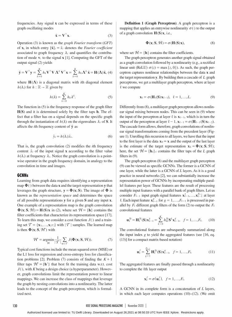
Layer 1 Layer 2

x z1 = H1(S)x z2 = H2(S)x1x1 = v(z1) x2 = v(z2)z1

x2 = U(x; S, H)x1

z2

FIGURE 1. Each blue block represents a linear graph filter and each green block represents a nonlinearity. The concatenation of a convolutional graph filter [cf. (2)] and a nonlinearity forms a graph perceptron (Definition 1) or layer. Using a bank of graph convolutional filters [cf. (10) and (11)] and cascad-ing several layers, leads to a GCNN. GCNNs are a subset of GNNs, which follow the same structure but consider arbitrary graph filters; see the section “Extensions: General Graph Filters.”


130 IEEE SIGNAL PROCESSING MAGAZINE | November 2020 |

frequencies. Any signal x can be expressed in terms of these graph oscillating modes

.V xx = <u (3)

Operation (3) is known as the graph Fourier transform (GFT) of x, in which entry [ ] xx i i=u u denotes the Fourier coefficient associated to graph frequency im and quantifies the contribu-tion of mode vi to the signal x [1]. Computing the GFT of the output signal (2) yields

( ) ,h hy V y V V V x x H xkk

k

Kk

kk

K

0 0

K K K= = = =< <<

= =

u u u/ / (4)

where ( )H K is a diagonal matrix with ith diagonal element ( )h im for :h RR " given by

( ) .h hkk

Kk

0

m m==

/ (5)

The function in (5) is the frequency response of the graph filter H(S) and it is determined solely by the filter taps h. The ef-fect that a filter has on a signal depends on the specific graph through the instantiation of ( )h m on the eigenvalues im of S. It affects the ith frequency content of yu as

( ) .y h xi i im=u u (6)

That is, the graph convolution (2) modifies the ith frequency content xiu of the input signal x according to the filter value

( )h im at frequency .im Notice the graph convolution is a point-wise operator in the graph frequency domain, in analogy to the convolution in time and images.

GCNNsLearning from graph data requires identifying a representation map ( )$U between the data x and the target representation y that leverages the graph structure, ( ; ).y x SU= The image of U is known as the representation space and determines the space of all possible representations y for a given S and any input x. One example of a representation map is the graph convolution

( ; , ) ( )x S H S xHU = in (2), where set { }hH = contains the filter coefficients that characterize its representation space [17]. To learn this map, we consider a cost function ( )J $ and a train-ing set { , , }x xT 1 Tf= ; ; with T; ; samples. The learned map is then ( ; , )x S HU ) with

( ( ; , )).argmin J1 x SHT

HxH T

U=)

!

/ (7)

Typical cost functions include the mean squared error (MSE) or the L1 loss for regression and cross-entropy loss for classifica-tion problems [2]. Problem (7) consists of finding the K 1+ filter taps { }hH =) ) that best fit the training data w.r.t. cost

( ),J $ with K being a design choice (a hyperparameter). Howev-er, graph convolutions limit the representation power to linear mappings. We can increase the class of mappings that leverage the graph by nesting convolutions into a nonlinearity. The latter leads to the concept of the graph perceptron, which is formal-ized next.

Definition 1 (Graph Perceptron). A graph perceptron is a mapping that applies an entrywise nonlinearity ( )$v to the output of a graph convolution ( ) ,H S x i.e.,

( ; , ) ( ( ) ),x S H S xH vU = (8)

where set { }hH = contains the filter coefficients.The graph perceptron generates another graph signal obtained

as a graph convolution followed by a nonlinearity (e.g., a rectified linear unit (ReLU) ( ) { , }).maxz z 0v = As such, the graph per-ceptron captures nonlinear relationships between the data x and the target representation y. By building then a cascade of L graph perceptrons, we get a multilayer graph perceptron, where at layer , we compute

( ( ) ), , , .L1x H S x 1 , fv= =, , ,- (9)

Differently from (8), a multilayer graph perceptron allows nonlin-ear signal mixing between nodes. This can be seen in (9) where the input of the perceptron at layer , is ,x 1,- which is in turn the output of the perceptron at layer , ( ( ) ).1 x H S x1 1 2, v- =, , ,- - - The cascade form allows, therefore, graph convolutions of nonlin-ear signal transformations coming from the precedent layer (Fig-ure 1). Unrolling this recursion to all layers, we have that the input to the first layer is the data x x0 = and the output of the last layer is the estimate of the target representation ( ; , );x x S HL U= here, the set { }hH = , , contains the filter taps of the L graph filters in (9).

The graph perceptron (8) and the multilayer graph perceptron (9) can be viewed as specific GCNNs. The former is a GCNN of one layer, while the latter is a GCNN of L layers. As it is a good practice in neural networks [2], we can substantially increase the representation power of GCNNs by incorporating multiple paral-lel features per layer. These features are the result of processing multiple input features with a parallel bank of graph filters. Let us consider F 1,- input graph signal features , ,x xF

11

11f, ,- -

,- at layer ., Each input feature xg

1,- for , ,g F1 1f= ,- is processed in par-allel by F, different graph filters of the form (2) to output the F, convolutional features

( ) , , , .h f F1u H S x S xfg fg gkfg

k

Kk g

10

1 f= = =, , , , , ,-=

-/ (10)

The convolutional features are subsequently summarized along the input index g to yield the aggregated features (see [16, eq. (13)] for a compact matrix-based notation)

( ) , , , .f F1u H S xf fg

g

Fg

11

1

f= =, , , ,

=-

,-

/ (11)

The aggregated features are finally passed through a nonlinearity to complete the th, layer output

, , , .f F1x uf ffv= =, , ,^ h (12)

A GCNN in its complete form is a concatenation of L layers, in which each layer computes operations (10)–(12). (We omit



pooling to emphasize the role of graph filters. Please refer to [5]–[7] for pooling methods.) Differently from the multilayer graph perceptron GCNN in (9), the complete form employs a parallel bank of F F 1#, ,- graph convolutional filters. This increases the representation power of the mapping and exploits both the stable operation in signal processing, the convolution, and the underly-ing graph structure of the data. The input to the first layer is the data x x0 = and the target representation is the collection of FL features of the last layer [ , , ] ( ; , ),x x x S HL L

F1 Lf U= where set { }hH fg

fg= , , collects now the filter taps of all layers. For a giv-en S and fixed hyperparameters L, ,F, and K, the representation space of a GCNN is characterized by the set of filter coefficients at each layer .H This representation space is different from the one obtained by using linear FIR filters representation maps [17]. (See “Implementations of GCNN.”)

We can learn the filter taps by solving (7) with the GCNN map ( ; , ).x S HU To do so, we use some optimization method based on stochastic gradient descent [18] and, noting the GCNN is a compositional layered architecture, we also use backpropa-gation to compute the derivatives of the loss function ( )J $ with respect to the filter taps H [19]. Since the training data comes from a distribution that has a graph structure S, we expect the

learned map ( ; , )x S HU ) to generalize and perform well for data x T" that come from a similar distribution leveraging S. The rationale behind this expectation is that the GCNN is a nonlin-ear processing architecture that exploits the knowledge the graph carries about the data. Another advantage of a GCNN is its local implementation due to the use of graph convolutions [cf. (2)] and pointwise nonlinearities. In fact, all the F F 1#, ,- convolutional features in (10) are local over the graph as they simply comprise a parallel bank of graph convolutional filters, each of which is local [cf. (2)]. Further, since the aggregation step in (11) happens across features of the same node and the nonlinearity in (12) is pointwise, these operations are also local and distributable. This built-in characteristic of GCNNs naturally leads to learning solu-tions that are distributed on the underlying graph. (See “Imple-mentations of GCNNs.”)

Permutation equivarianceA graph shift operator S fixes an arbitrary ordering of the nodes in the graph. Since nodes are naturally unordered, we want the GCNN output to be unaffected by it. That is, we want any change in node ordering to be reflected with the corresponding reordering in the GCNN output. It turns out GCNNs are unaffected by node

Given a matrix representation S and fixed set of hyperparameters [number of layers ,L filter taps ,K features F, and nonlinearity ( )$v ], the representation space of the graph convolutional neural network (GCNN) model (10)–(12) is characterized by the set of parameters H that determine the graph filters. There exist in the literature different implementations for the graph convolution operation (10), as well as other parametrizations that further restrict this representation space. We overview these in light of the description (10)–(12).Same representation spaceSpectral GCNNs [5] compute (10) in the spectral domain (4) and consider the (normalized) Laplacian as the shift ;Sas long as all the eigenvalues of S are different, both (4) and (10) are equivalent [1]. ChebNets [6] use a Chebyshev polynomial to compute the graph convolution and consider as S a normalized version of the Laplacian that forces all eigenvalues to be in [ , ]1 1- which is re quired for the use of Chebyshev polynomials; Chebsyhev polynomials are equivalent to the polynomials in (10). In summary, we see that [5] and [6] just differ in their implementation of the graph convolution, but all cover the same representation space as the GCNN model (10)–(12) for the specific shift .SSmaller representation spaceGCNs [8] consider (10) with only the onehop filter tap h fg

1, for each layer and each filter, i.e., K 1= and h 0fg

0 =, for all ;, they adopt a normalized selflooped

version of the adjacency as .S Simple graph convolutional networks (SGCs) [9] consider (10) with only the Khop filter tap, i.e., h 0k

fg =, for all ;k K1 they also adopt a normalized selflooped version of the adjacency as .S Graph isomorphism networks (GINs) [10] consider an orderone polynomial K 1= but with ( )h h1fg fg

0 1f= +, , , for some predefined ;f, it adopts the binary adjacency as S and suggests the inclusion of layers with K 0= in between layers with .K 1= Diffusion CNNs [11] consider a single layer with F NF1 0= and the same K filter taps for all input features

;h hkfg

kf

1 1= it adopts the adjacency matrix as .S It follows that the representations space of [8]–[11] is just a subspace of the representation space of the GCNN model in (10)–(12).

We note that, while the representation space of [5] and [6] is the same as in the GCNN model (10)–(12), their difference in the implementation of the graph convolution impacts how the optimization space is navigated during training, arriving at different solutions. No particular implementation, however, has consistently outperformed the rest across a wide range of problems. In any case, since the representation space is the same, the characterizations, properties and insights established here apply to all of these. Implementations [8]–[11], on the other hand, further regularize the graph convolution, constraining the representation space to be a subspace of that in the GCNN model. These might be useful in problems with smaller data sets, or where further information on the data structure is available.

Implementations of GCNNs



labeling—a property known as permutation equivariance—as stated by the following theorem. [12], [13]

Theorem 1 (Permutation Equivariance). Consider an N N# permutation matrix P and the permutations of the shift operator S P SP= <t and of the input data .x P x= <t For a GCNN

( )$U [12], [13], it holds that [12], [13]

( ; , ) ( ; , ).x P x SS H HU U= <t t (13)

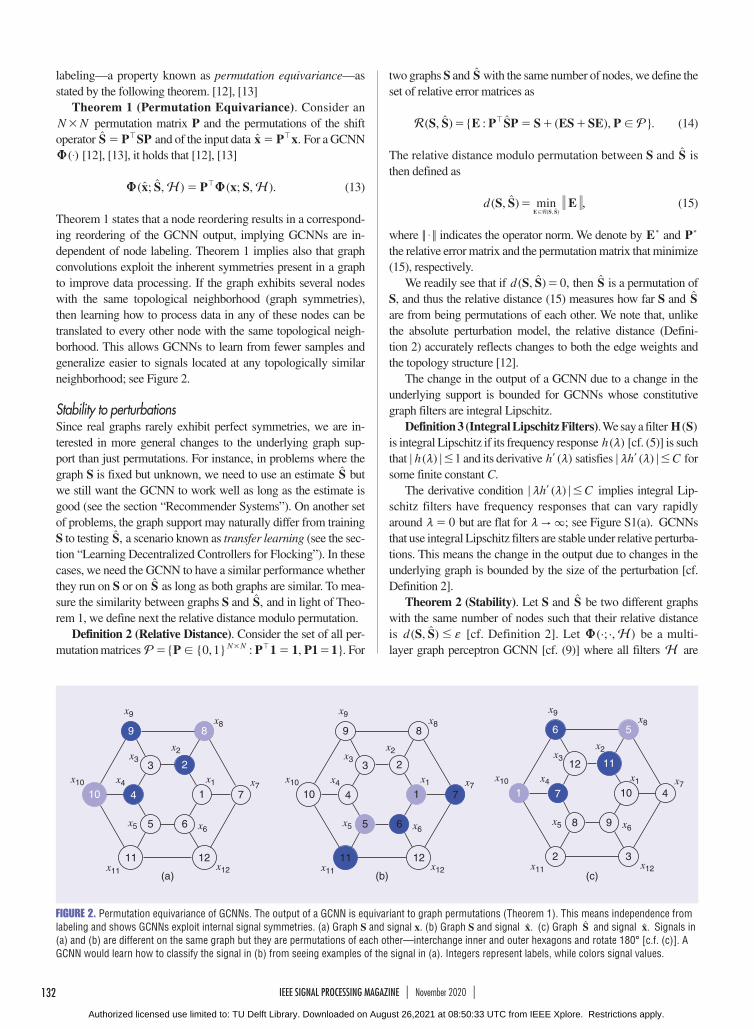
Theorem 1 states that a node reordering results in a correspond-ing reordering of the GCNN output, implying GCNNs are in-dependent of node labeling. Theorem 1 implies also that graph convolutions exploit the inherent symmetries present in a graph to improve data processing. If the graph exhibits several nodes with the same topological neighborhood (graph symmetries), then learning how to process data in any of these nodes can be translated to every other node with the same topological neigh-borhood. This allows GCNNs to learn from fewer samples and generalize easier to signals located at any topologically similar neighborhood; see Figure 2.

Stability to perturbationsSince real graphs rarely exhibit perfect symmetries, we are in-terested in more general changes to the underlying graph sup-port than just permutations. For instance, in problems where the graph S is fixed but unknown, we need to use an estimate St but we still want the GCNN to work well as long as the estimate is good (see the section “Recommender Systems”). On another set of problems, the graph support may naturally differ from training S to testing ,St a scenario known as transfer learning (see the sec-tion “Learning Decentralized Controllers for Flocking”). In these cases, we need the GCNN to have a similar performance whether they run on S or on St as long as both graphs are similar. To mea-sure the similarity between graphs S and ,St and in light of Theo-rem 1, we define next the relative distance modulo permutation.

Definition 2 (Relative Distance). Consider the set of all per-mutation matrices { { , } : , }.0 1 1 1 1P P 1 PP N N!= = =# < For

two graphs S and St with the same number of nodes, we define the set of relative error matrices as

( , ) { : ( ), }.S E P SP S ES SE PSR P!= = + +<t t (14)

The relative distance modulo permutation between S and St is then defined as

( , ) ,mind S ES( , )E S SR

=!

tt

(15)

where $< < indicates the operator norm. We denote by E) and P) the relative error matrix and the permutation matrix that minimize (15), respectively.

We readily see that if ( , ) ,d 0S S =t then St is a permutation of S, and thus the relative distance (15) measures how far S and St are from being permutations of each other. We note that, unlike the absolute perturbation model, the relative distance (Defini-tion 2) accurately reflects changes to both the edge weights and the topology structure [12].

The change in the output of a GCNN due to a change in the underlying support is bounded for GCNNs whose constitutive graph filters are integral Lipschitz.

Definition 3 (Integral Lipschitz Filters). We say a filter ( )H S is integral Lipschitz if its frequency response ( )h m [cf. (5)] is such that ( )h 1; ; #m and its derivative ( )h ml satisfies ( )h C; ; #m ml for some finite constant C.

The derivative condition ( )h C; ; #m ml implies integral Lip-schitz filters have frequency responses that can vary rapidly around 0m = but are flat for ;" 3m see Figure S1(a). GCNNs that use integral Lipschitz filters are stable under relative perturba-tions. This means the change in the output due to changes in the underlying graph is bounded by the size of the perturbation [cf. Definition 2].

Theorem 2 (Stability). Let S and St be two different graphs with the same number of nodes such that their relative distance is ( , )d S S # ft [cf. Definition 2]. Let (·; ·, )HU be a multi-layer graph perceptron GCNN [cf. (9)] where all filters H are

1

23

4

5 6

7

89

10x10

x5

x4

x3

x6

x9x8

x7x1

x2

x12x11

11 12

1

23

4

5 6

7

89

10x10

x5

x4

x3

x6

x9x8

x7x1

x2

x12x11

11 12

10

1112

7

8 9

4

56

1x10

x5

x4

x3

x6

x9x8

x7x1

x2

x12x11

2 3

(a) (b) (c)

FIGURE 2. Permutation equivariance of GCNNs. The output of a GCNN is equivariant to graph permutations (Theorem 1). This means independence from labeling and shows GCNNs exploit internal signal symmetries. (a) Graph S and signal x. (b) Graph S and signal .xt (c) Graph St and signal .xt Signals in (a) and (b) are different on the same graph but they are permutations of each other—interchange inner and outer hexagons and rotate 180° [c.f. (c)]. A GCNN would learn how to classify the signal in (b) from seeing examples of the signal in (a). Integers represent labels, while colors signal values.



integral Lipschitz with constant C [cf. Definition 3]. Then, it holds that [12]

; , ; ,

,C N L2 1

x S P x P SP

x

H H

O 2# d f f

U U-

+ +

) ) )< < t^^

^^

hh

hh

(16)

where ( )1 1U V 2< <d = - + - is the eigenvector misalignment between the eigenbasis V of S and the eigenbasis U of the relative error matrix ,E) with E) and P) given in Definition 2.

Theorem 2 proves that a change f in the shift operator causes a change proportional to f in the GCNN output. The proportion-ality constant has the term C that depends on the filter design, and the term ( )N1 d+ that depends on the specific perturba-tion. But it also has a constant factor L that depends on the depth of the architecture implying deeper GCNNs are less stable. (See “Insights on Stability.”)

Extensions: General graph filtersOftentimes, the GCNN would require highly sharp filter re-sponses to discriminate between classes. We can increase the discriminatory power by either increasing the filter order K or changing the filter type H(S) in the graph perceptron (8). In-creasing K is not always feasible as it leads to more filter coeffi-cients, a higher complexity, and numerical issues related to the higher order powers of the shift operator .Sk Instead, changing the filter type allows implementing another family of GNNs with different properties. We present two alternative filters that provide different insights on how to design more general GNNs: the ARMA graph filter [14] and the edge-varying graph filter [15].

ARMANetAn ARMA graph filter operates also pointwise in the spectral do-main ( )y h xi i im=u u [cf. (6)] but it is characterized by the rational frequency response

( ) .ha

b

1 pp

qq

p

Pq

Q

1

0m

m

m

=+

=

=

/

/ (17)

The frequency response is now controlled by P denominator coefficients [ , , ]a aa P1 f= < and Q 1+ numerator coefficients

[ , , ] .b bb Q0 f= < The rational frequency responses in (17) span an equivalent space to that of graph filters in (2). However, the spectral equivalence does not imply that the two filters have the same properties. ARMA filters implement rational frequency re-sponses rather than polynomial ones as FIR filters do (5). There-fore, we expect them to achieve a sharper response with lower orders of P and Q such that .P Q K1+ Replacing the spectral variable m with the shift operator S allows us to write the ARMA output ( )y H S x= as

: ,a by I S S x P S Q S xpp

Pp

qq

Qq

1

1

0

1= + ==

-

=

-e e ^ ^o o h h/ / (18)

where ( ) : aP S I SpP

pp

1R= + = and : bQ SqQ q

0 1R= = are two FIR filters [cf. (2)] that allow writing the ARMA filter as ( )H S =

( ) ( ).P S Q S1- As it follows from (18), we need to apply the ma-trix inverse P(S) to obtain the ARMA output. This, unless the number of nodes is moderate, is computationally unaffordable; hence, we need an iterative method to approximately apply the inverse. Due to its faster convergence, we choose a parallel struc-ture that consists of first transforming the polynomial ratio in (18) into its partial fraction decomposition form and subsequently us-ing the Jacobi method to approximately apply the inverse. While other Krylov approaches are also possible to solve (18), the paral-lel Jacobi method offers a better tradeoff between computational complexity, distributed implementation, and convergence.

Partial fraction decomposition of ARMA filtersConsider the rational frequency response ( )h m in (17) and let

[ , , ]P1 fc c c= < be the P poles, [ , , ]P1 fb b b= < the corre-sponding residuals and [ , , ]K0 fa a a= < the direct terms. Then, we can write (18) in the equivalent form

.y S I x S xpp

P

p kk

Kk

1

1

0

b c a= - +=

-

=

^ h/ / (19)

The equivalence of (19) and (18) implies that instead of learning a and b in (18), we can learn , ,a b and c in (19). To avoid the matrix inverses in the single pole filters, we can approximate each output u p through the Jacobi method.

Jacobi method for single pole filtersWe can write the output of the pth single pole filter u p in the equivalent linear equation form ( ) .S I u xp p pc b- = The Jacobi algorithm requires separating ( )S Ipc- into its diagonal and off-diagonal terms. Defining ( )diagD S= as the matrix containing the diagonal of the shift operator, we can write the Jacobi approxi-mation u px of the pth single pole filter output u p at iteration x by the recursive expression

, .withu D I x S D u u x( )p p p p p1

1 0c b= - - - =x x-

-^ ^h h6 @ (20)

The inverse in (20) is now elementwise on the diagonal matrix ( ).D Ipc- This recursion can be unrolled to all its terms to write an explicit relationship between u px and .x To do that, we define the parameterized shift operator ( ) ( ) ( )R D I S Dp p

1c c=- - -- and use it to write the Tth Jacobi recursion as

( ) ( ) .u R x R xpT p

T

pT

p0

1

b c c= +x

x=

-

/ (21)

For a convergent Jacobi method, u pT converges to the single pole output .u p However, in a practical setting we truncate (21) for a finite T. We can then write the single pole filter output as

: ( ( )) ,u H R xpT T pc= where we define the following FIR filter of order T:

( ( )) ( ) ( )H R R RT p p

T

pT

p0

1

c b c c= +x

x=

-

/ (22)

with the parametric shift operator ( ).R c In other words, a single pole filter is approximated by a graph convolutional filter of the



form (2) in which the shift operator S is substituted by ( ).R c This parametric convolutional filter uses coefficients pb for , ,T0 1fx = - and 1 for .Tx =

Jacobi ARMA filters and ARMANetsAssuming we use truncated Jacobi iterations of order T to ap-proximate all single pole filters in (19), we can write the ARMA filter as

( ) ( ( )) ,H S H R STp

P

p kk

Kk

1 0

c a= += =

/ / (23)

where the pth approximated single pole filter ( ( ))H RT pc is de-fined in (22) and the parametric shift operator ( )R pc in (21). In summary, a Jacobi approximation of the ARMA filter with orders (P, T, K) is the one defined by (22) and (23). Scalar P indicates the number of poles, T the number of Jacobi iterations, and K the order of the direct term Sk

Kk

k0aR = in (19).

Substituting (23) into (8) yields an ARMA graph percep-tron, which is the building block for ARMA GNNs or, for short, ARMANets. ARMANets are themselves convolutional. For a sufficiently large number of Jacobi iterations T, (23) is equivalent to (18) which performs a pointwise multiplication in the spectral

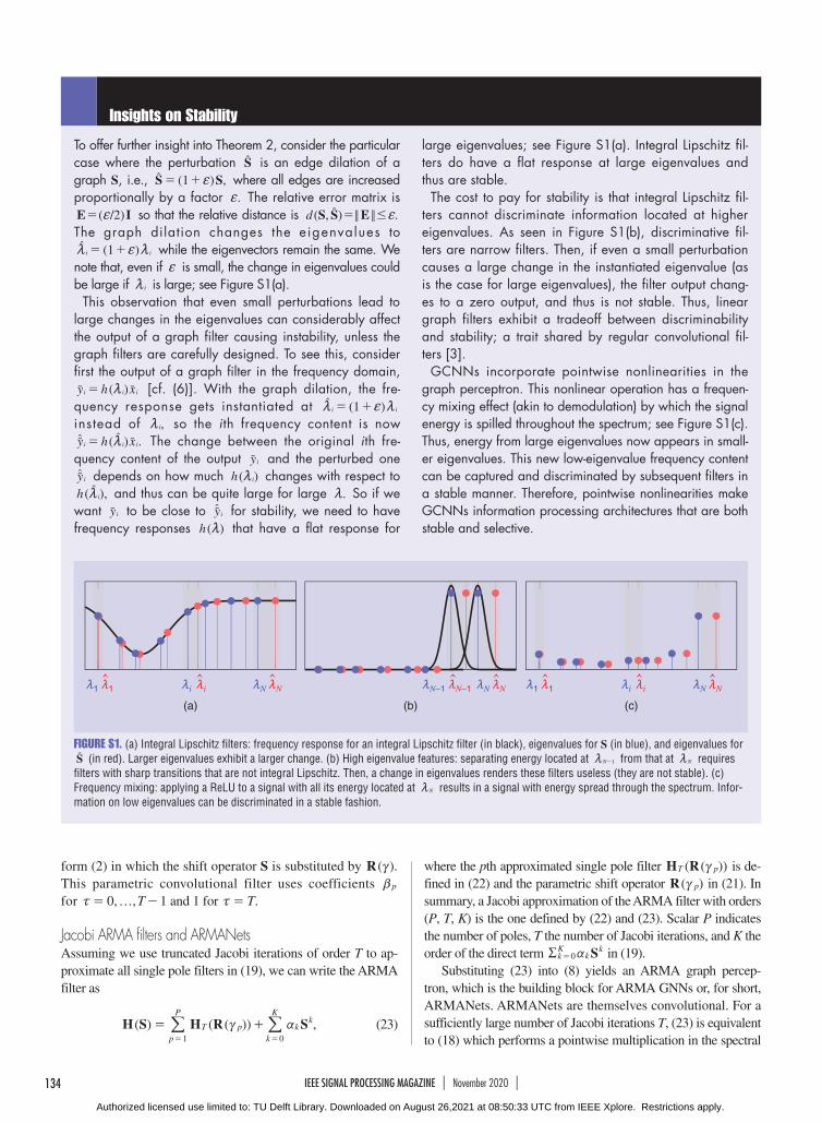
To offer further insight into Theorem 2, consider the particular case where the perturbation St is an edge dilation of a graph S, i.e., ( )1 ,S Sf= +t where all edges are increased proportionally by a factor .f The relative error matrix is

( / )2E If= so that the relative distance is ( , ) .d S S E< <#f=t The graph dilation changes the eigenvalues to

( )1i im f m= +t while the eigenvectors remain the same. We note that, even if f is small, the change in eigenvalues could be large if im is large; see Figure S1(a).

This observation that even small perturbations lead to large changes in the eigenvalues can considerably affect the output of a graph filter causing instability, unless the graph filters are carefully designed. To see this, consider first the output of a graph filter in the frequency domain,

( )y h xi i im=u u [cf. (6)]. With the graph dilation, the frequency response gets instantiated at ( )1i im f m= +t instead of ,im so the ith frequency content is now

( ) .y h xi i im=ut t u The change between the original ith frequency content of the output yiu and the perturbed one yiut depends on how much ( )h im changes with respect to

( ),h imt and thus can be quite large for large .m So if we want yiu to be close to yiut for stability, we need to have frequency responses ( )h m that have a flat response for

large eigenvalues; see Figure S1(a). Integral Lipschitz filters do have a flat response at large eigenvalues and thus are stable.

The cost to pay for stability is that integral Lipschitz filters cannot discriminate information located at higher eigenvalues. As seen in Figure S1(b), discriminative filters are narrow filters. Then, if even a small perturbation causes a large change in the instantiated eigenvalue (as is the case for large eigenvalues), the filter output changes to a zero output, and thus is not stable. Thus, linear graph filters exhibit a tradeoff between discriminability and stability; a trait shared by regular convolutional filters [3].

GCNNs incorporate pointwise nonlinearities in the graph perceptron. This nonlinear operation has a frequency mixing effect (akin to demodulation) by which the signal energy is spilled throughout the spectrum; see Figure S1(c). Thus, energy from large eigenvalues now appears in smaller eigenvalues. This new loweigenvalue frequency content can be captured and discriminated by subsequent filters in a stable manner. Therefore, pointwise nonlinearities make GCNNs information processing architectures that are both stable and selective.

Insights on Stability

m1 m1

"

m1 m1

"

mi mi

"

mi mi

"

mN mN

"

mN mN

"

mN mN

"

mN–1 mN–1

"

(a) (b) (c)

FIGURE S1. (a) Integral Lipschitz filters: frequency response for an integral Lipschitz filter (in black), eigenvalues for S (in blue), and eigenvalues for St (in red). Larger eigenvalues exhibit a larger change. (b) High eigenvalue features: separating energy located at N 1m - from that at Nm requires filters with sharp transitions that are not integral Lipschitz. Then, a change in eigenvalues renders these filters useless (they are not stable). (c) Frequency mixing: applying a ReLU to a signal with all its energy located at Nm results in a signal with energy spread through the spectrum. Infor-mation on low eigenvalues can be discriminated in a stable fashion.



domain with the response (17). The Jacobi filters in (23) are also reminiscent of the convolutional filters in (2). But the similarity is superficial because in ARMANets we train also the P2 single pole filter coefficients pb and pc alongside the K 1+ coefficients of the direct term .Sk

Kk

K0aR = The equivalence suggests ARMA-

Nets may help achieve more discriminatory filters by tuning the single pole filter orders P and T. An example of an implementa-tion of ARMANets are CayleyNets [20]; see [16].

EdgeNetWhile ARMANets enhance the discriminatory power of GCNNs with alternative convolutional filters, the edge-varying GNN de-parts from the convolutional prior to improve GCNNs. The Ed-geNet leverages the sparsity and locality of the shift operator S and forms a graph perceptron [cf. (9)] by replacing the graph con-volutional filter with an edge-varying graph filter [15].

From shared to edge parametersIn the convolutional filter (2), all nodes share the same scalar hk to weigh equally the information from all k-hop away neighbors

.S xk This is advantageous because it limits the number of train-able parameters, allows permutation equivariance, and favors stability. However, this parameter sharing limits also the discrimi-natory power to architectures whose filters H(S) have the same eigenvectors as S [cf. (4)]. We can improve the discriminatory power by considering a linear filter in which node i uses a scalar

( )ijkU to weigh the information of its neighbor j at iteration k. For

,k 0= each node weighs only its own signal to build the zero-shifted signal ,z x( ) ( )0 0U= where ( )0U is an N N# diagonal ma-trix of parameters with ith diagonal entry ( )

ii0U being the weight

of node i. Signal z( )0 is subsequently exchanged with neighboring nodes to build the one-shifted signal ,z z( ) ( ) ( )1 1 0U= where the parameter matrix ( )1U shares the support with ;I S+ the (i, j)th entry ( )

ij1U is the weight node i applies to signal z( )

j0 from neigh-

bor j. Repeating the latter for k shifts, we get the recursion

, , , ,k K0z z x x( ) ( ) ( ) ( ) ( : )k k k k

k

kk1

0

0 fU U U= = = =-

=

l

l

% (24)

where the product matrix ( : ) ( ) ( ) ( )kkk k k0

00gPU U U U= ==l

l ac-counts for the weighted propagation of the graph signal z x( )1 =- from at most k-hops away neighbors. Each node is therefore free to adapt its weights for each iteration k to capture the necessary local detail.

Edge-varying filters and EdgeNetsThe collection of signals z( )k in (24) behaves like a sequence of parametric shifts, where at iteration k we use the parametric shift operator ( )kU to shift-and-weigh the signal. Following the same idea as in (2), we can sum up edge-varying shifted signals z( )k to get the input–output map ( )y H xU= of an edge-varying graph filter. For this relation to hold, the filter matrix ( )H U should satisfy

( ) .H ( : )k

k

Kk

k

k

k

K0

0 00

U U U= == ==

l

le o%/ / (25)

The edge-varying graph filter is characterized by the K 1+ pa-rameter matrices , ,( ) ( )K0 fU U and contains ( )K M N N+ +

parameters. The edge-varying graph filter forms the broadest family of graph filters: It generalizes the FIR filter in (2) (for

),h S( : )kk

k0U = the ARMA filter in (23), and almost all other fil-ters employed to build GNNs including spectral filters [5], Che-byshev filters [6], Cayley filters, graph isomorphism filters, and also graph attention filters [21].

Substituting (25) into (8) yields an edge-varying graph per-ceptron, which is the building block for edge-varying GNNs or, for short, EdgeNets. EdgeNets are more than convolutional architectures; the high number of degrees of freedom and lin-ear complexity render EdgeNets strong candidates for highly discriminatory GNNs in sparse graphs. If the graph is large, the EdgeNet can efficiently trade some edge detail (e.g., allowing edge-varying weights only to a few nodes) to make the num-ber of parameters independent of the graph dimension [16]. To control the number of parameters in EdgeNets we can adopt graph attention networks [21]; see [16] for details on this and other alternatives.

ApplicationsWe consider the application of GNNs for rating prediction in rec-ommender systems (see the section “Recommender Systems”) and learning decentralized controllers for flocking (see the sec-tion “Learning Decentralized Controllers for Flocking”). These two applications aim at illustrating the use of GNNs in problems beyond semisupervised learning.

We focus on the representation space of GNNs built with different filter types and compare them with that of linear FIR filters to corroborate the discussed insights. We note that, in all cases, the values of hyperparameters (number of layers L, filter taps K, and features )F, are design choices that have been made after cross-validation. (The PyTorch GNN library used is avail-able at http://github.com/alelab-upenn/graph-neural-networks.)

Recommender systemsConsider the problem of rating prediction in recommender sys-tems. We have a database of users that have rated many items, and we use it to build a graph where each item is a node and each edge weight is given by the rating similarity between items [22]. Then, given the ratings a specific user has given to some of the items, we want to predict the rating the same user would give to a specific item not yet rated. The ratings given by that user can be modeled as a graph signal, so that this becomes a problem of interpolating one of the (unknown) entries in it.

SetupWe consider items as movies and use a subset of the MovieLens-100k data set, containing the 200 movies with the largest number of ratings [23]. The resulting data set has 47,825 ratings given by 943 users to some of those 200 movies. The similarity between movies is the Pearson correlation [22, eq. (6)], which is further sparsified to keep only the ten edges with the stronger similarity. We split the data set into 90% for training and 10% for testing. In this context, each user represents a graph signal, where the value at each node is the rating given to that movie. Movies not rated are given a value of zero. The objective is to estimate the rating a



user would give to the movie Star Wars based on the ratings given by that same user to other movies and leveraging the graph of rating similarities.

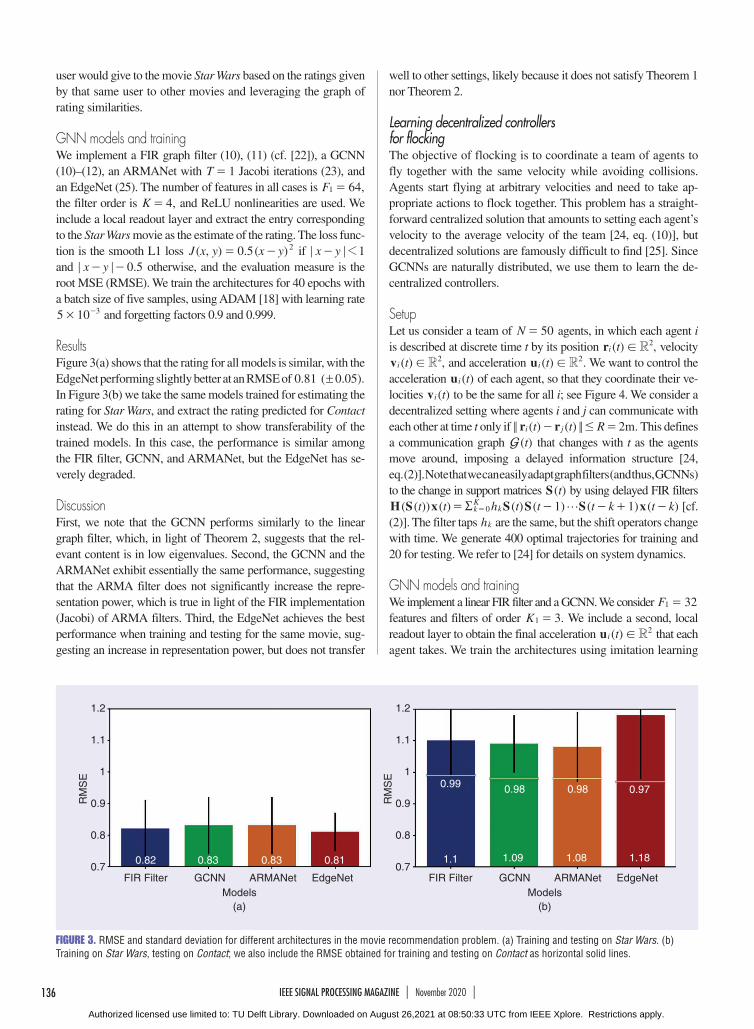
GNN models and trainingWe implement a FIR graph filter (10), (11) (cf. [22]), a GCNN (10)–(12), an ARMANet with T 1= Jacobi iterations (23), and an EdgeNet (25). The number of features in all cases is ,F 641 = the filter order is ,K 4= and ReLU nonlinearities are used. We include a local readout layer and extract the entry corresponding to the Star Wars movie as the estimate of the rating. The loss func-tion is the smooth L1 loss ( , ) . ( )J x y x y0 5 2= - if x y 11; ;- and .x y 0 5; ;- - otherwise, and the evaluation measure is the root MSE (RMSE). We train the architectures for 40 epochs with a batch size of five samples, using ADAM [18] with learning rate 5 10 3# - and forgetting factors 0.9 and 0.999.

ResultsFigure 3(a) shows that the rating for all models is similar, with the EdgeNet performing slightly better at an RMSE of . ( . ).0 81 0 05! In Figure 3(b) we take the same models trained for estimating the rating for Star Wars, and extract the rating predicted for Contact instead. We do this in an attempt to show transferability of the trained models. In this case, the performance is similar among the FIR filter, GCNN, and ARMANet, but the EdgeNet has se-verely degraded.

DiscussionFirst, we note that the GCNN performs similarly to the linear graph filter, which, in light of Theorem 2, suggests that the rel-evant content is in low eigenvalues. Second, the GCNN and the ARMANet exhibit essentially the same performance, suggesting that the ARMA filter does not significantly increase the repre-sentation power, which is true in light of the FIR implementation (Jacobi) of ARMA filters. Third, the EdgeNet achieves the best performance when training and testing for the same movie, sug-gesting an increase in representation power, but does not transfer

well to other settings, likely because it does not satisfy Theorem 1 nor Theorem 2.

Learning decentralized controllers for flockingThe objective of flocking is to coordinate a team of agents to fly together with the same velocity while avoiding collisions. Agents start flying at arbitrary velocities and need to take ap-propriate actions to flock together. This problem has a straight-forward centralized solution that amounts to setting each agent’s velocity to the average velocity of the team [24, eq. (10)], but decentralized solutions are famously difficult to find [25]. Since GCNNs are naturally distributed, we use them to learn the de-centralized controllers.

SetupLet us consider a team of N 50= agents, in which each agent i is described at discrete time t by its position ( ) ,tr Ri

2! velocity ( ) ,tv Ri

2! and acceleration ( ) .tu Ri2! We want to control the

acceleration ( )tui of each agent, so that they coordinate their ve-locities ( )tvi to be the same for all i; see Figure 4. We consider a decentralized setting where agents i and j can communicate with each other at time t only if ( ) ( ) .t t R 2mr ri j< < #- = This defines a communication graph ( )tG that changes with t as the agents move around, imposing a delayed information structure [24, eq. (2)]. Note that we can easily adapt graph filters (and thus, GCNNs) to the change in support matrices ( )tS by using delayed FIR filters

( ( )) ( ) ( ) ( ) ( ) ( )t t h t t t k t k1 1H S x S S S xkK

k0 gR= - - + -= [cf. (2)]. The filter taps hk are the same, but the shift operators change with time. We generate 400 optimal trajectories for training and 20 for testing. We refer to [24] for details on system dynamics.

GNN models and trainingWe implement a linear FIR filter and a GCNN. We consider F 321 = features and filters of order .K 31 = We include a second, local readout layer to obtain the final acceleration ( )tu Ri

2! that each agent takes. We train the architectures using imitation learning

1.2

1.1

1

0.9

0.8

0.7

RM

SE

GCNNFIR Filter ARMANet EdgeNetModels

0.82 0.83 0.810.83

1.2

1.1

1

0.9

0.8

0.7

RM

SE

GCNNFIR Filter ARMANet EdgeNetModels

(a) (b)

0.99

1.1

0.98 0.98 0.97

1.09 1.181.08

FIGURE 3. RMSE and standard deviation for different architectures in the movie recommendation problem. (a) Training and testing on Star Wars. (b) Training on Star Wars, testing on Contact; we also include the RMSE obtained for training and testing on Contact as horizontal solid lines.



by minimizing the MSE between the out-put action ( )tui and the optimal action

( )tui) given by [24, eq. (10)]. At test time,

we do not require access to the optimal action. The evaluation measure is the ve-locity variation of the team throughout the trajectory, ( ) ( )N t tv vt i

Ni

11

2< <R R --= r

with ( ) ( )t N tv vjN

j1

1R= -=r being the av-

erage velocity at time t. We trained for 40 epochs with a batch size of 20 samples using ADAM [18] with learning rate 5 10 4# - and forgetting factors 0.9 and 0.999.

ResultsWe observe in Table 1 the cost achieved by the GCNN-based con-troller is close to the optimal cost, while the FIR filter fails to con-trol the system leading to a very high cost. We further investigate the effect of Theorems 1 and 2 by transferring at scale the learned solutions. That is, we take the controllers learned with teams of N 50= agents, and test them in teams of increasing size. The GCNN scales perfectly, maintaining the same performance.

DiscussionsThe GCNNs improved performance over the graph filter is ex-pected since we know that optimal distributed controllers are non-linear [25]. The GCNN also achieves a cost close to optimum, evidencing successful control. Once trained, this GCNN based controller can be used in teams of arbitrary number of agents evi-dencing the properties of permutation equivariance and stability, and speaking to the potential of GCNNs for learning behaviors in homogenous teams.

ConclusionsGSP plays a crucial role in characterizing and understanding the representation space of GNNs. By emphasizing the role of graph filters and leveraging the concept of GFT, we are able to derive fundamental properties such as permutation equivariance and stability, as well as establish a unified mathematical description.

This reinforces the notion that GNNs are nonlinear extensions of graph filters, and thus GSP can help explain and understand the observed success of GNNs and contribute to improved designs.

As a matter of fact, several areas of interest lie ahead for GSP researchers to pursue. First, the understanding of what precise effect the nonlinearities have on the frequency content is limited. A better characterization of their effect in relation to the underlying topology is bound to help in designing appropriate ones. Second, the gen-eral relationship between the hyperparameters (number of layers, filter taps) and the characteristics of the graph (diameter, degree) is currently unknown. It is expected, for instance, the number of hops bears some relationship with the diameter of the graph, but no theoretical result is out there yet. Third, the bounds in the stability results are quite loose due to the coarse bound used on the eigenvec-tors. Thus, focusing on the eigenvector perturbation to improve the bound is a worthwhile pursuit. Fourth, the stability result holds for graphs of the same size. Extending this result to graphs of different size is an important research direction. Finally, we mention explor-ing the possibility of nonlinear aggregations of the filter banks, as well as using different shift operators at each layer.

From a higher vantage point, realizing GNNs are an object of study of GSP and regarding them as nonlinear extensions of graph filters, help us exploit our understanding of filtering techniques as well as leverage spectral domain analysis. Thus, GSP plays a cru-cial role in characterizing, understanding, and improving GNNs.

AcknowledgmentsThe work described in this article was supported by National Sci-ence Foundation Computing and Communication Foundations

(a) (b) (c)

FIGURE 4. Snapshots of a sample trajectory. The dots illustrate the agents, the gray edges represent the communication links, and the arrows show the velocity. (a) The agents start flying at time t 0 s= with arbitrary velocities. (b) They manage to agree on a direction at .t 1s= (c) They effectively fly together at .t 2 s=

Table 1. Scalability results. These models were trained on 50 agents and tested on N agents. Optimal cost: 51(± 1).

N 50 62 75 87 100 FIR filter ( )408 88! ( )408 93! ( )434 128! ( )420 105! ( )430 131!

GCNN ( )77 3! ( )78 3! ( )77 2! ( )77 2! ( )78 2!



grant 1717120, Army Research Office grant W911NF1710438, and Army Research Laboratory Distributed and Collaborative Intelligent Systems and Technology Collaborative Research Alli-ance grant W911NF-17-2-0181 and by the International Science and Technology Center-Wireless Autonomous Systems and Intel DevCloud. Fernando Gama is the corresponding author.

AuthorsFernando Gama ([email protected]) received his electronic engineer degree from the University of Buenos Aires, Argentina, in 2013; his M.A. degree in statistics from the Wharton School, University of Pennsylvania, Philadelphia, in 2017; and his Ph.D. degree in electrical and systems engineering from the University of Pennsylvania in 2020. He has been a visiting researcher at the Delft University of Technology, The Netherlands, in 2017, and a research intern at Facebook Artificial Intelligence Research, Montréal, in 2018. He was awarded a Fulbright scholarship for international students. His research interests lie in the areas of information processing and machine learning for network data.

Elvin Isufi ([email protected]) received his Ph.D. degree from the Delft University of Technology, The Netherlands, in 2019. He was a postdoctoral researcher with the Department of Electrical and Systems Engineering, University of Pennsylvania, Philadelphia, and is currently an assistant professor with the Multimedia Computing Group, Delft University of Technology where he is also the codirector of AidroLab—the lab of artificial intelligence on water network. His research interests include the intersection of signal processing, mathematical modeling, machine learning, and network theory.

Geert Leus ([email protected]) received his M.Sc. and Ph.D. degrees in electrical engineering from the Katholieke Universiteit Leuven, Belgium, in June 1996 and May 2000, respectively. He is now a professor at the Faculty of Electrical Engineering, Mathematics and Computer Science of the Delft University of Technology, The Netherlands. He received a 2002 IEEE Signal Processing Society Young Author Best Paper Award and a 2005 IEEE Signal Processing Society Best Paper Award. Currently, he is the chair of the European Association for Signal Processing (EURASIP) Special Area Team on Signal Processing for Multisensor Systems, and the editor in chief of EURASIP Signal Processing. His research interests are in the broad area of signal processing, with a specific focus on wireless communications, array processing, sensor networks, and graph signal processing. He is a Fellow of IEEE and EURASIP.

Alejandro Ribeiro ([email protected]) received his B.Sc. degree in electrical engineering from the Universidad de la Republica Oriental del Uruguay, Montevideo, in 1998 and the M.Sc. and his Ph.D. degrees in electrical engineering from the Department of Electrical and Computer Engineering, the University of Minnesota, Minneapolis, in 2005 and 2007, respectively. He is currently a professor of electrical and systems engineering at the University of Pennsylvania, Philadelphia. He received an Outstanding Research Award from Intel in 2019, the 2014 O. Hugo Schuck Best Paper Award, and various confer-ence and workshop paper awards. He is a Fulbright and a University of Pennsylvania fellow.

References[1] A. Ortega, P. Frossard, J. Kovacˇevic´, J. M. F. Moura, and P. Vandergheynst, “Graph signal processing: Overview, challenges and applications,” Proc. IEEE, vol. 106, no. 5, pp. 808–828, May 2018. doi: 10.1109/JPROC.2018.2820126.

[2] I. Goodfellow, Y. Bengio, and A. Courville, Deep Learning (The Adaptive Computation and Machine Learning Series). Cambridge, MA: MIT Press, 2016.

[3] S. Mallat, “Group invariant scattering,” Commun. Pure, Appl. Math., vol. 65, no. 10, pp. 1331–1398, Oct. 2012. doi: 10.1002/cpa.21413.

[4] M. M. Bronstein, J. Bruna, Y. LeCun, A. Szlam, and P. Vandergheynst, “Geometric deep learning: Going beyond Euclidean data,” IEEE Signal Process. Mag., vol. 34, no. 4, pp. 18–42, July 2017. doi: 10.1109/MSP.2017.2693418.

[5] J. Bruna, W. Zaremba, A. Szlam, and Y. LeCun, “Spectral networks and deep locally connected networks on graphs,” in Proc. 2nd Int. Conf. Learning Representations, Banff, AB, Apr. 14–16, 2014, pp. 1–14.

[6] M. Defferrard, X. Bresson, and P. Vandergheynst, “Convolutional neural networks on graphs with fast localized spectral filtering,” in Proc. 30th Conf. Neural Information Processing Systems, Barcelona, Spain, Dec. 5–10, 2016, pp. 3844–3858. doi: 10.5555/3157382.3157527.

[7] F. Gama, A. G. Marques, G. Leus, and A. Ribeiro, “Convolutional neural network architectures for signals supported on graphs,” IEEE Trans. Signal Process., vol. 67, no. 4, pp. 1034–1049, Feb. 2019. doi: 10.1109/TSP.2018.2887403.

[8] T. N. Kipf and M. Welling, “Semi-supervised classification with graph convolutional networks,” in Proc. 5th Int. Conf. Learning Representations, Toulon, France, Apr. 24–26, 2017, pp. 1–14.

[9] F. Wu, A. Souza, T. Zhang, C. Fifty, T. Yu, and K. Weinberger, “Simplifying graph convolutional networks,” in Proc. 36th Int. Conf. Machine Learning, vol. 97. Long Beach, CA: PMLR, June 9–15, 2019, pp. 6861–6871.

[10] K. Xu, W. Hu, J. Leskovec, and S. Jegelka, “How powerful are graph neural net-works?” in Proc. 7th Int. Conf. Learning Representations, New Orleans, LA, May 6–9, 2019, pp. 1–17.

[11] J. Atwood and D. Towsley, “Diffusion-convolutional neural networks,” in Proc. 30th Conf. Neural Information Processing Systems, Barcelona, Spain, Dec. 5–10, 2016, pp. 2001–2009. doi: 10.5555/3157096.3157320.

[12] F. Gama, J. Bruna, and A. Ribeiro, “Stability properties of graph neural networks,” July 8, 2020. [Online]. Available: http://arXiv:1905.04497

[13] D. Zou and G. Lerman, “Graph convolutional neural networks via scattering,” Appl. Comput. Harmon. Anal., vol. 49, no. 3, pp. 1046–1074, Nov. 2020. doi: 10.1016/j.acha.2019.06.003.

[14] E. Isufi, A. Loukas, A. Simonetto, and G. Leus, “Autoregressive moving average graph filtering,” IEEE Trans. Signal Process., vol. 65, no. 2, pp. 274–288, Jan. 2017. doi: 10.1109/TSP.2016.2614793.

[15] M. Coutino, E. Isufi, and G. Leus, “Advances in distributed graph filtering,” IEEE Trans. Signal Process., vol. 67, no. 9, pp. 2320–2333, May 2019. doi: 10.1109/TSP.2019.2904925.

[16] E. Isufi, F. Gama, and A. Ribeiro, “EdgeNets: Edge varying graph neural net-works,” Mar. 12, 2020. [Online]. Available: http://arXiv:2001.07620

[17] M. Püschel and J. M. F. Moura, “Algebraic signal processing theory: Foundation and 1-D time,” IEEE Trans. Signal Process., vol. 56, no. 8, pp. 3575–3585, Aug. 2008. doi: 10.1109/TSP.2008.925261.

[18] D. P. Kingma and J. L. Ba, “ADAM: A method for stochastic optimization,” in Proc. 3rd Int. Conf. Learning Representations, San Diego, CA, May 7–9, 2015, pp. 1–15.

[19] D. E. Rumelhart, G. E. Hinton, and R. J. Williams, “Learning representations by back-propagating errors,” Nature, vol. 323, no. 6088, pp. 533–536, Oct. 1986. doi: 10.1038/323533a0.

[20] R. Levie, F. Monti, X. Bresson, and M. M. Bronstein, “CayleyNets: Graph convo-lutional neural networks with complex rational spectral filters,” IEEE Trans. Signal Process., vol. 67, no. 1, pp. 97–109, Jan. 2019. doi: 10.1109/TSP.2018.2879624.

[21] P. Velicˇkovic´, G. Cucurull, A. Casanova, A. Romero, P. Liò, and Y. Bengio, “Graph attention networks,” in Proc. 6th Int. Conf. Learning Representations, Vancouver, BC, Apr./May 2018, pp. 1–12.

[22] W. Huang, A. G. Marques, and A. Ribeiro, “Rating prediction via graph signal pro-cessing,” IEEE Trans. Signal Process., vol. 66, no. 19, pp. 5066–5081, Oct. 2018. doi: 10.1109/TSP.2018.2864654.

[23] F. M. Harper and J. A. Konstan, “The MovieLens datasets: History and context,” ACM Trans. Interactive Intell. Syst., vol. 5, no. 4, Jan. 2016, Art. no. 19. doi: 10.1145/2827872.

[24] E. Tolstaya, F. Gama, J. Paulos, G. Pappas, V. Kumar, and A. Ribeiro, “Learning decentralized controllers for robot swarms with graph neural networks,” in Proc. Conf. Robot Learning 2019, Osaka, Japan, pp. 671–682.

[25] H. S. Witsenhausen, “A counterexample in stochastic optimum control,” SIAM J. Control, vol. 6, no. 1, pp. 131–147, 1968. doi: 10.1137/0306011.

SP


Graphs, Convolutions, and Neural Networks: From Graph ...

Documents

Transcript of Graphs, Convolutions, and Neural Networks: From Graph ...