Graphs 1 Last Update: Dec 4, 2014. Graphs A graph is a pair (V, E), where – V is a set of nodes,...
140
Graphs Graphs 1 Last Update: Dec 4, 2014
-
Upload
jennifer-walker -
Category
Documents
-
view
214 -
download
1
Transcript of Graphs 1 Last Update: Dec 4, 2014. Graphs A graph is a pair (V, E), where – V is a set of nodes,...
Graphs
Graphs 1Last Update: Dec 4, 2014

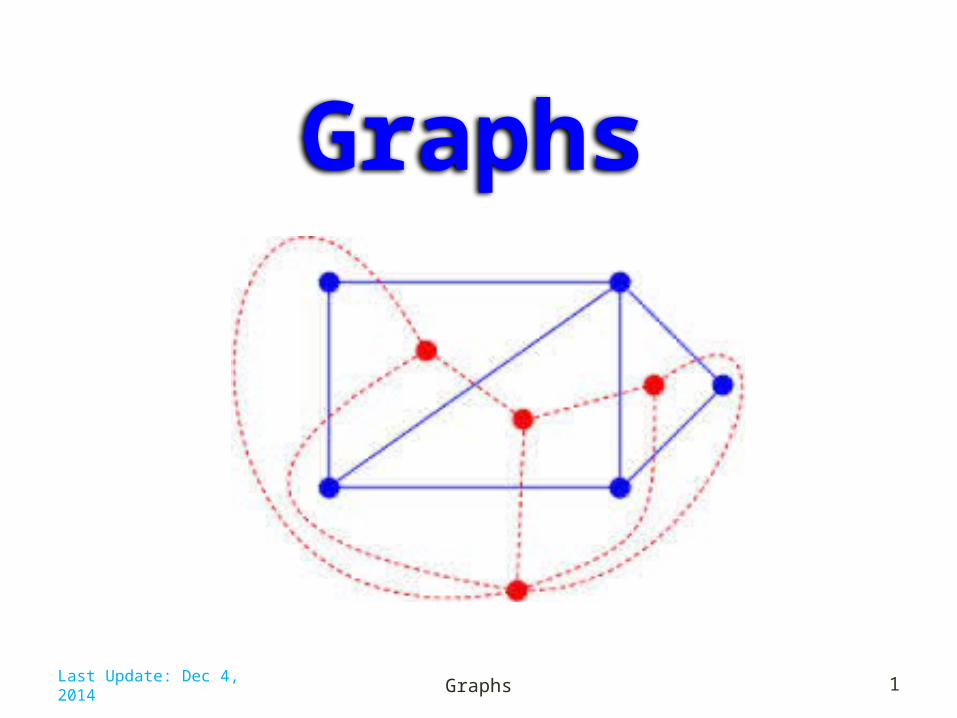
Graphs• A graph is a pair (V, E), where
– V is a set of nodes, called vertices– E is a collection of pairs of vertices, called edges– Vertices and edges are positions and store elements
• Example:– A vertex represents an airport and stores the three-letter airport code– An edge represents a flight route between two airports and stores the
mileage of the route
Graphs 2
ORD PVD
MIADFW
SFO
LAX
LGA
HNL
849
802
13871743
1843
10991120
1233337
2555
142
Last Update: Dec 4, 2014
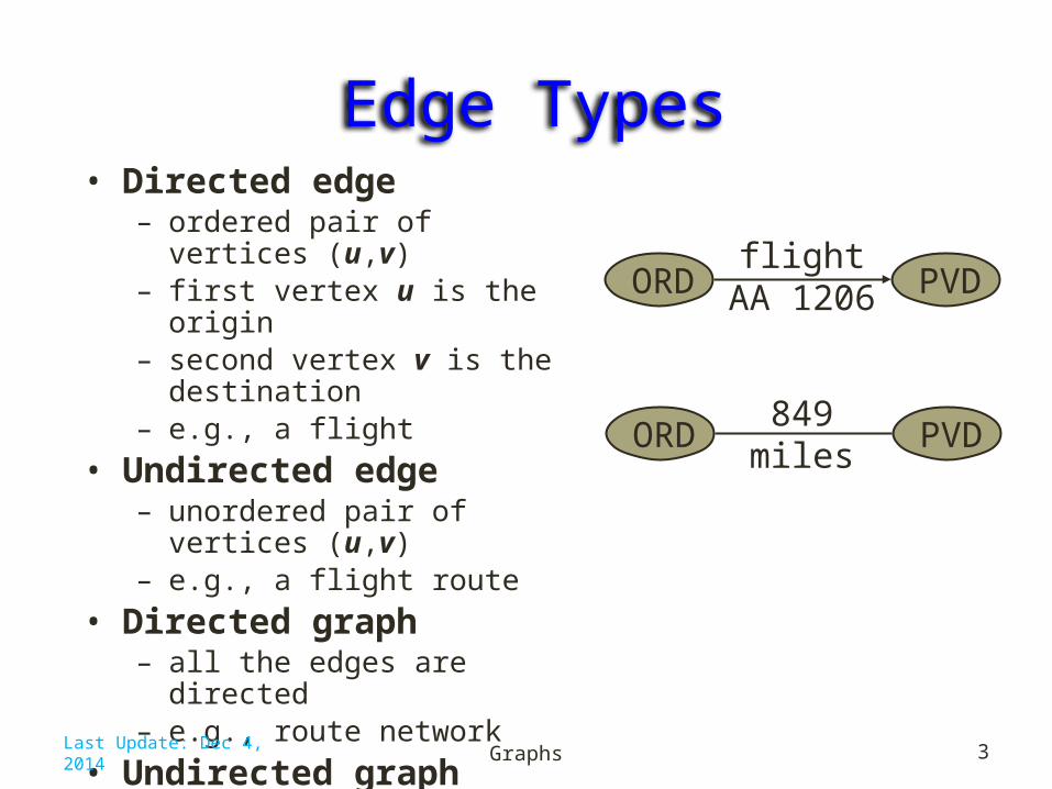
Edge Types• Directed edge
– ordered pair of vertices (u,v)– first vertex u is the origin– second vertex v is the destination– e.g., a flight
• Undirected edge– unordered pair of vertices (u,v)– e.g., a flight route
• Directed graph– all the edges are directed– e.g., route network
• Undirected graph– all the edges are undirected– e.g., flight network
Graphs 3
ORD PVDflight
AA 1206
ORD PVD849
miles
Last Update: Dec 4, 2014
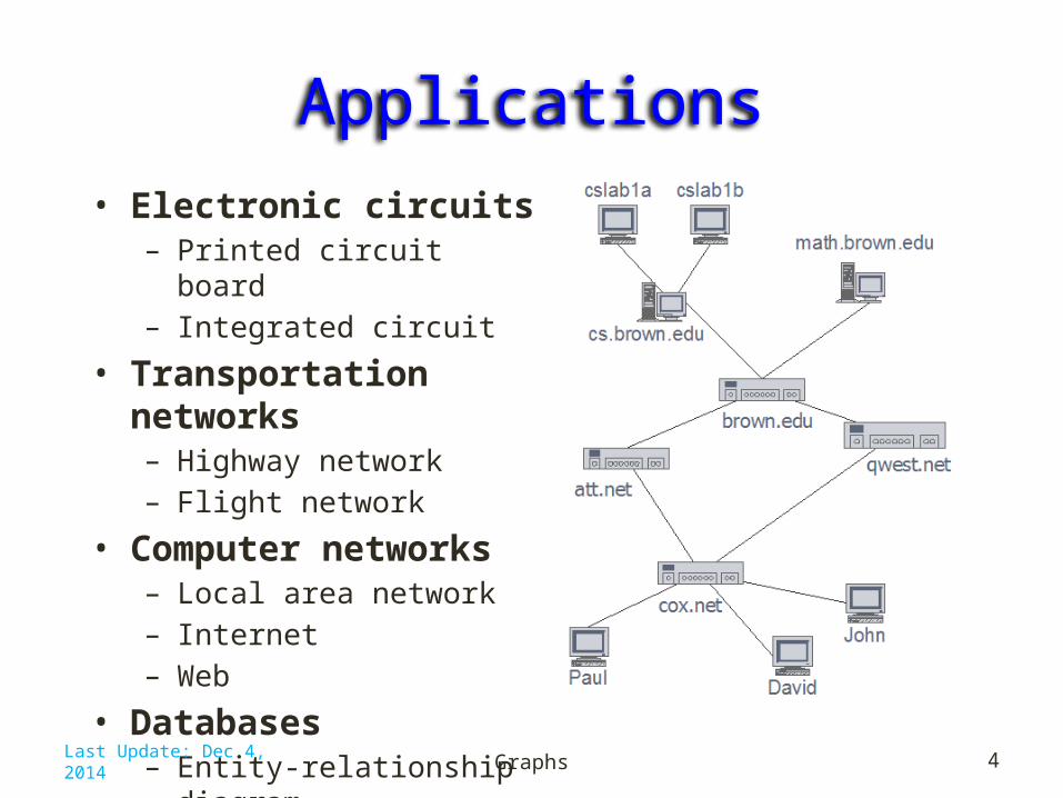
Applications• Electronic circuits
– Printed circuit board– Integrated circuit
• Transportation networks– Highway network– Flight network
• Computer networks– Local area network– Internet– Web
• Databases– Entity-relationship diagram
Graphs 4Last Update: Dec 4, 2014

Terminology• End vertices (or endpoints) of an edge
– U and V are the endpoints of a• Edges incident on a vertex
– a, d, and b are incident on V• Adjacent vertices
– U and V are adjacent• Degree of a vertex
– X has degree 5 • Parallel edges
– h and i are parallel edges• Self-loop
– j is a self-loop
Graphs 5
XU
V
W
Z
Y
a
c
b
e
d
f
g
h
i
j
Last Update: Dec 4, 2014
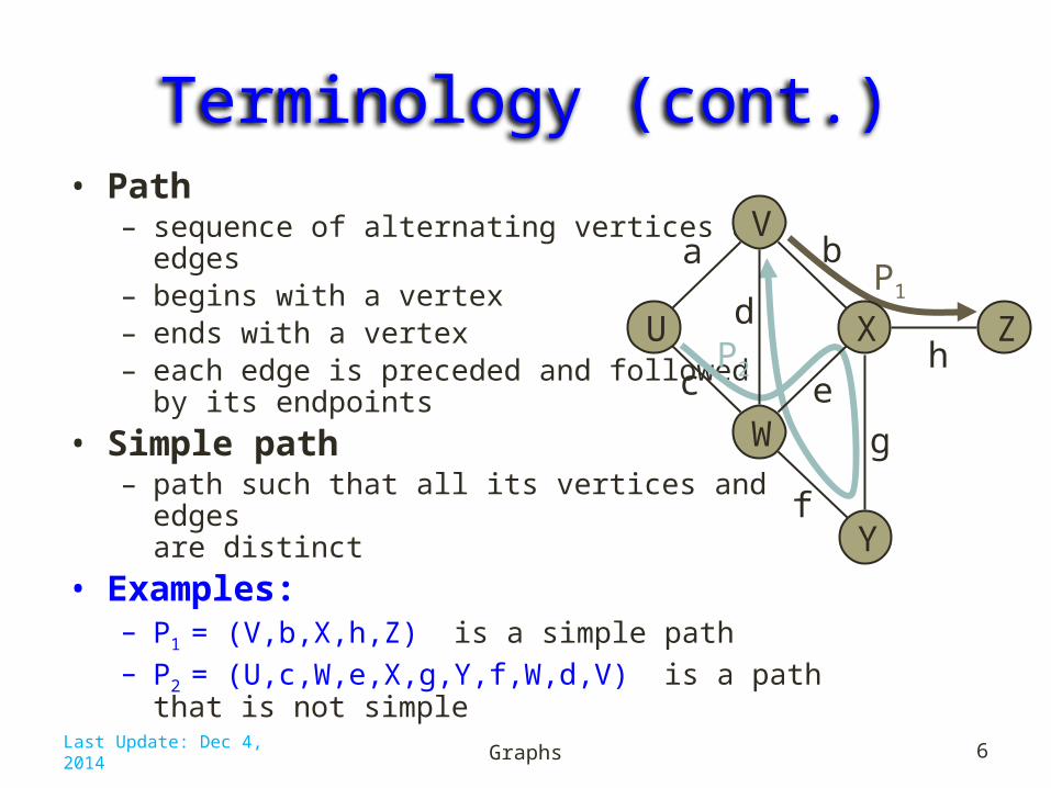
Terminology (cont.)• Path
– sequence of alternating vertices and edges – begins with a vertex– ends with a vertex– each edge is preceded and followed
by its endpoints• Simple path
– path such that all its vertices and edges are distinct
• Examples:– P1 = (V,b,X,h,Z) is a simple path– P2 = (U,c,W,e,X,g,Y,f,W,d,V) is a path that is not simple
Graphs 6
P1
XU
V
W
Z
Y
a
c
b
e
d
f
g
hP2
Last Update: Dec 4, 2014
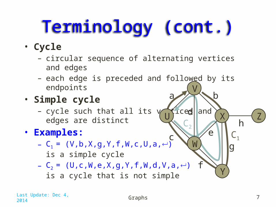
Terminology (cont.)• Cycle
– circular sequence of alternating vertices and edges – each edge is preceded and followed by its endpoints
• Simple cycle– cycle such that all its vertices and
edges are distinct
• Examples:– C1 = (V,b,X,g,Y,f,W,c,U,a,)
is a simple cycle– C2 = (U,c,W,e,X,g,Y,f,W,d,V,a,)
is a cycle that is not simple
Graphs 7
C1
XU
V
W
Z
Y
a
c
b
e
d
f
g
hC2
Last Update: Dec 4, 2014

PropertiesNotation
n number of vertices m number of edgesdeg(v) degree of vertex v
Property 1v deg(v) = 2mProof: each edge is counted twice
Property 2In an undirected graph with no self-loops and
no multiple edges m n (n - 1)/2Proof: each vertex has degree at most (n - 1)
What is the bound for a directed graph?
Graphs 8Last Update: Dec 4, 2014

Vertices and Edges• A graph is a collection of vertices and edges. • We model the abstraction as a combination of three data
types: Vertex, Edge, and Graph. • A Vertex is a lightweight object that stores an arbitrary
element provided by the user (e.g., an airport code)– We assume it supports a method, element(), to retrieve the stored
element.
• An Edge stores an associated object (e.g., a flight number, travel distance, cost), retrieved with the element( ) method.
Graphs 9Last Update: Dec 4, 2014
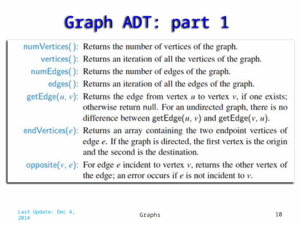
Graph ADT: part 1
Graphs 10Last Update: Dec 4, 2014
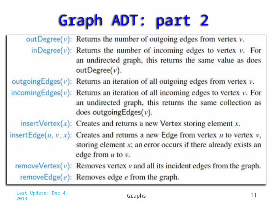
Graph ADT: part 2
Graphs 11Last Update: Dec 4, 2014

Edge List Structure
Graphs 12Last Update: Dec 4, 2014
• Vertex object– element– reference to position in vertex sequence
• Edge object– element– origin vertex object– destination vertex object– reference to position in edge sequence
• Vertex sequence– sequence of vertex objects
• Edge sequence– sequence of edge objects

Adjacency List Structure
Graphs 13Last Update: Dec 4, 2014
• Incidence sequence for each vertex– sequence of references to edge objects
of incident edges
• Augmented edge objects– references to associated positions in
incidence sequences of end vertices

Adjacency Map Structure
Graphs 14Last Update: Dec 4, 2014
• Incidence sequence for each vertex– sequence of references to adjacent
vertices, each mapped to edge object of the incident edge
• Augmented edge objects– references to associated positions in
incidence sequences of end vertices

Adjacency Matrix Structure
Graphs 15Last Update: Dec 4, 2014
• Edge list structure• Augmented vertex objects
– Integer key (index) associated with vertex• 2D-array adjacency array
– Reference to edge object for adjacent vertices– Null for non-adjacent vertices
• The “old fashioned” version just has0 for no edge and 1 for edge
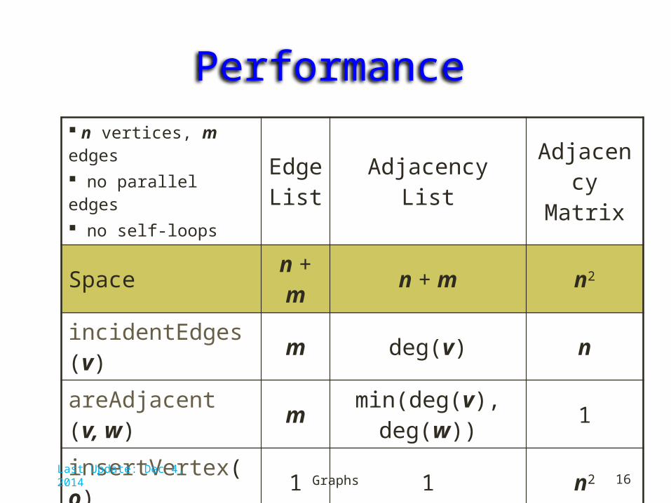
Performance n vertices, m edges no parallel edges no self-loops
EdgeList
AdjacencyList
Adjacency Matrix
Space n + m n + m n2
incidentEdges(v) m deg(v) nareAdjacent (v, w) m min(deg(v), deg(w)) 1insertVertex(o) 1 1 n2
insertEdge(v, w, o) 1 1 1removeVertex(v) m deg(v) n2
removeEdge(e) 1 max(deg(v), deg(w)) 1
Graphs 16Last Update: Dec 4, 2014

Subgraphs• A subgraph S of a graph G is a graph such that – The vertices of S are a subset of the vertices of G– The edges of S are a subset of the edges of G
• A spanning subgraph of G is a subgraph that contains all the vertices of G
Graphs 17
Subgraph Spanning subgraph
Last Update: Dec 4, 2014

Connectivity• A graph is connected if there is a path between every
pair of vertices• A connected component of a graph G is a maximal
connected subgraph of G
Graphs 18
Connected graphNon connected graph with
two connected components
Last Update: Dec 4, 2014
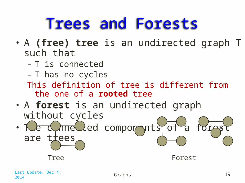
Trees and Forests• A (free) tree is an undirected graph T such that– T is connected– T has no cyclesThis definition of tree is different from the one of a rooted tree
• A forest is an undirected graph without cycles• The connected components of a forest are trees
Graphs 19
Tree Forest
Last Update: Dec 4, 2014

Spanning Trees and Forests• A spanning tree of a connected graph is a spanning
subgraph that is a tree• A spanning tree is not unique unless the graph is a tree• Spanning trees have applications to the design of
communication networks• A spanning forest of a graph is a spanning subgraph
that is a forest
Graphs 20
Graph Spanning tree
Last Update: Dec 4, 2014
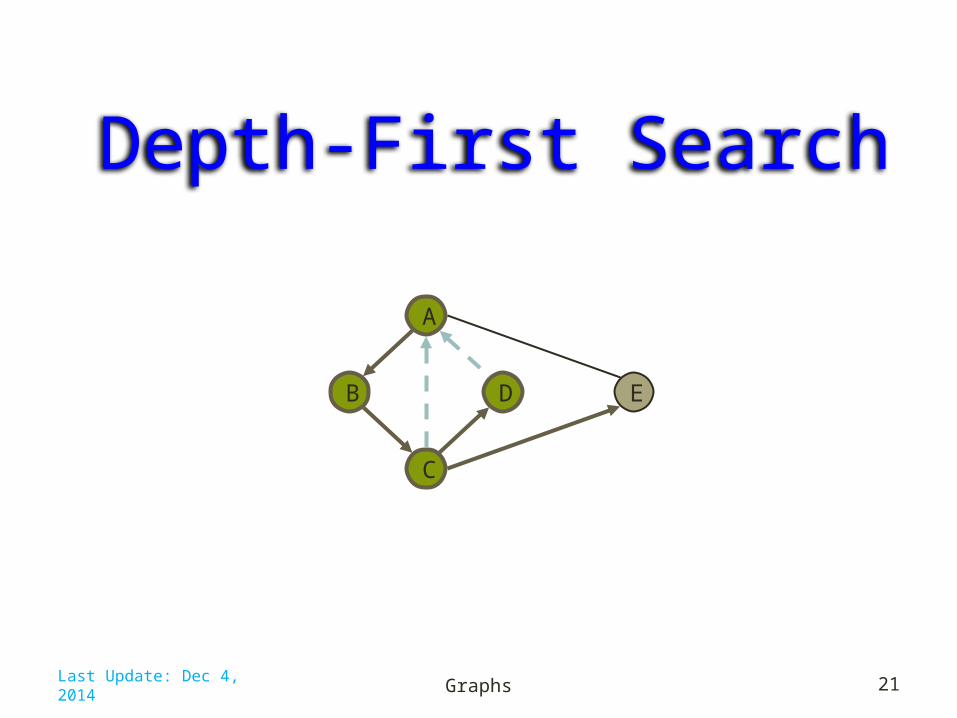
Depth-First Search
Graphs 21
DB
A
C
E
Last Update: Dec 4, 2014

Depth-First Search• DFS is a general graph traversal
technique
• DFS(G) – Visits all the vertices and edges of G– Determines whether G is connected– Computes the connected
components of G– Computes a spanning forest of G
• DFS on a graph with n vertices and m edges takes O(n + m ) time
• DFS can be further extended to solve other graph problems– Find and report a path
between two given vertices– Find a cycle in the graph
• Depth-first search is to graphs what Euler tour is to binary trees
Graphs 22Last Update: Dec 4, 2014

DFS Algorithm from a Vertex
Graphs 23Last Update: Dec 4, 2014

Java Implementation
Graphs 24Last Update: Dec 4, 2014

Example
Graphs 25
DB
A
C
E
DB
A
C
E
DB
A
C
E
discovery edgeback edge
A visited vertexA unexplored vertex
unexplored edge
Last Update: Dec 4, 2014

DB
A
C
E
Example (cont.)
Graphs 26
DB
A
C
E DB
A
C
E
DB
A
C
E
Last Update: Dec 4, 2014
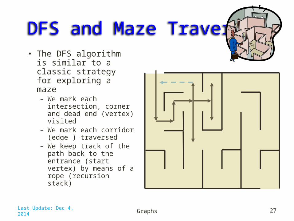
DFS and Maze Traversal • The DFS algorithm is
similar to a classic strategy for exploring a maze– We mark each
intersection, corner and dead end (vertex) visited
– We mark each corridor (edge ) traversed
– We keep track of the path back to the entrance (start vertex) by means of a rope (recursion stack)
Graphs 27Last Update: Dec 4, 2014

Properties of DFSProperty 1: DFS(G, v) visits all the vertices and edges
in the connected component of v
Property 2: The discovery edges labeled by DFS(G, v) form a spanning tree of the connected component of v
Graphs 28
DB
A
C
E
Last Update: Dec 4, 2014

Analysis of DFS• Setting/getting a vertex/edge label takes O(1) time• Each vertex is labeled twice
– once as UNEXPLORED– once as VISITED
• Each edge is labeled twice– once as UNEXPLORED– once as DISCOVERY or BACK (for undirected graphs)
• Method incidentEdges is called once for each vertex• DFS runs in O(n + m) time provided the graph is
represented by the adjacency list structure– Recall that v deg(v) = 2m
Graphs 29Last Update: Dec 4, 2014
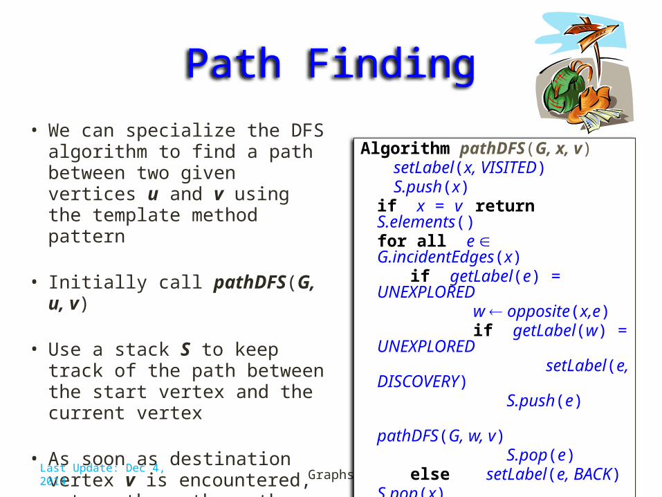
Path Finding• We can specialize the DFS algorithm
to find a path between two given vertices u and v using the template method pattern
• Initially call pathDFS(G, u, v)
• Use a stack S to keep track of the path between the start vertex and the current vertex
• As soon as destination vertex v is encountered, return the path as the contents of the stack
Graphs 30
Algorithm pathDFS(G, x, v)setLabel(x, VISITED)S.push(x)
if x = v return S.elements()for all e G.incidentEdges(x)
if getLabel(e) = UNEXPLORED
w opposite(x,e)
if getLabel(w) = UNEXPLORED
setLabel(e, DISCOVERY)
S.push(e)
pathDFS(G, w, v)
S.pop(e)
else setLabel(e, BACK)S.pop(x)
Last Update: Dec 4, 2014

Path Finding in Java
Graphs 31Last Update: Dec 4, 2014

Cycle Finding• We can specialize the DFS algorithm
to find a simple cycle using the template method pattern
• Use a stack S to keep track of the path between the start vertex and the current vertex v
• As soon as a back edge (v, w) is encountered, return the cycle as the portion of the stack from the top vertex v to vertex w
Graphs 32
Algorithm cycleDFS(G, v)setLabel(v, VISITED)S.push(v)
for all e G.incidentEdges(v)if getLabel(e) =
UNEXPLORED w opposite(v,e) S.push(e) if getLabel(w) =
UNEXPLORED
setLabel(e, DISCOVERY)
cycleDFS(G, w)
S.pop(e) else
T new empty stack
repeat
o S.pop()
T.push(o)
until o = w
return T.elements()S.pop(v)
Last Update: Dec 4, 2014
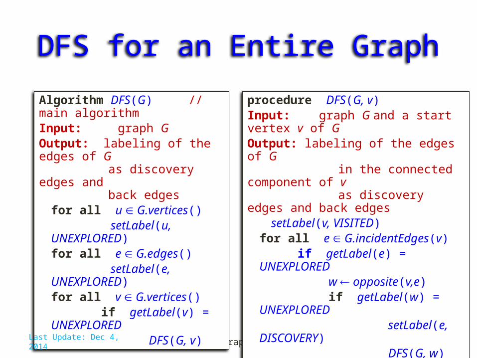
DFS for an Entire Graph
Graphs 33
procedure DFS(G, v)Input: graph G and a start vertex v of G Output: labeling of the edges of G
in the connected component of v
as discovery edges and back edges
setLabel(v, VISITED)for all e G.incidentEdges(v)
if getLabel(e) = UNEXPLORED w opposite(v,e) if getLabel(w) =
UNEXPLORED
setLabel(e, DISCOVERY) DFS(G,
w) else
setLabel(e, BACK)
Algorithm DFS(G) // main algorithmInput: graph GOutput: labeling of the edges of G
as discovery edges and
back edgesfor all u G.vertices()
setLabel(u, UNEXPLORED)for all e G.edges()
setLabel(e, UNEXPLORED)for all v G.vertices() if getLabel(v) = UNEXPLORED
DFS(G, v)
Last Update: Dec 4, 2014
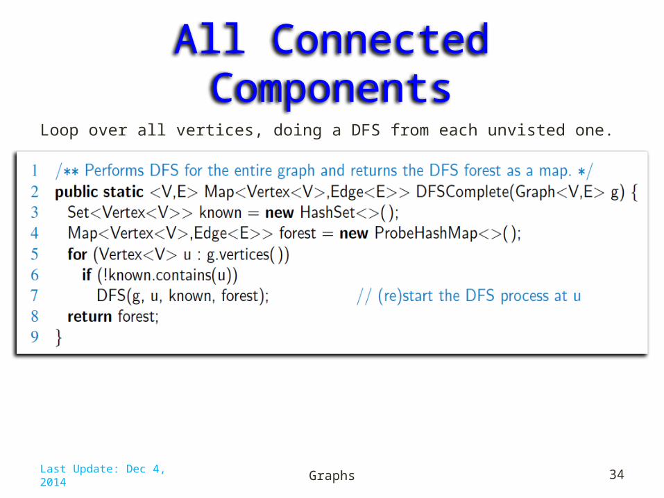
All Connected ComponentsLoop over all vertices, doing a DFS from each unvisted one.
Graphs 34Last Update: Dec 4, 2014
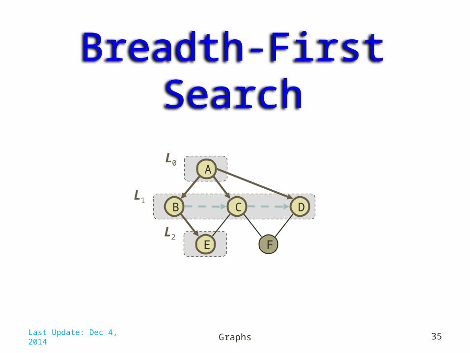
Breadth-First Search
Graphs 35
CB
A
E
D
L0
L1
FL2
Last Update: Dec 4, 2014

Breadth-First Search• BFS is a general graph traversal
technique
• A BFS traversal of a graph G – Visits all vertices and edges of G– Determines whether G is connected– Computes connected components of G– Computes a spanning forest of G
• BFS takes O(n + m ) time
• BFS can be extended to solve other graph problems, e.g.,
– Find a path with minimum number of edges between two given vertices
– Find a simple cycle, if there is one
Graphs 36Last Update: Dec 4, 2014

BFS Algorithm• The algorithm uses a
mechanism for setting and getting “labels” of vertices and edges
• Assume all vertices and edges of G are initialized to “UNEXPLORED”
• BFS(G, s) will partition all vertices reachable from s in G into levels
Graphs 37
procedure BFS(G, s)i 0 Li new empty queue
Li . enque(s)setLabel(s, VISITED)while Li . isEmpty()
Li+1 new empty queue // next level
for all v Li . elements() for all e
G.incidentEdges(v) if getLabel(e)
= UNEXPLORED w
opposite(v,e) if
getLabel(w) = UNEXPLORED
setLabel(e, DISCOVERY)
setLabel(w, VISITED)
Li +1 . enque(w) else
setLabel(e, CROSS) i i +1 // start next level
explorationend-while
Last Update: Dec 4, 2014
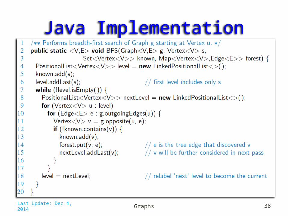
Java Implementation
Graphs 38Last Update: Dec 4, 2014

Example
Graphs 39
discovery edgecross edge
A visited vertexA unexplored vertex
unexplored edge
CB
A
E
D
L0
L1
F
CB
A
E
D
L0
L1
F
CB
A
E
D
L0
L1
F
Last Update: Dec 4, 2014

Example (cont.)
Graphs 40
CB
A
E
D
L0
L1
F
CB
A
E
D
L0
L1
FL2
CB
A
E
D
L0
L1
FL2
CB
A
E
D
L0
L1
FL2
Last Update: Dec 4, 2014
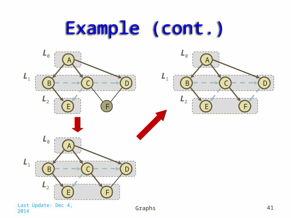
Example (cont.)
Graphs 41
CB
A
E
D
L0
L1
FL2
CB
A
E
D
L0
L1
FL2
CB
A
E
D
L0
L1
FL2
Last Update: Dec 4, 2014

PropertiesNotation: Gs = connected component of sProperty 1: BFS(G, s) visits all the vertices and edges of Gs Property 2: Discovery edges labeled by BFS(G, s) form
a spanning tree Ts of Gs
Property 3: For each vertex v in level Li
– The path of Ts from s to v has i edges – Every path from s to v in Gs has at least i edges
Graphs 42
CB
A
E
D
L0
L1
FL2
CB
A
E
D
F
Last Update: Dec 4, 2014

Analysis• Setting/getting a vertex/edge label takes O(1) time• Each vertex is labeled twice
– once as UNEXPLORED– once as VISITED
• Each edge is labeled twice– once as UNEXPLORED– once as DISCOVERY or CROSS
• Each vertex is inserted once into a sequence Li • Method incidentEdges is called once for each vertex• BFS runs in O(n + m) time provided the graph is
represented by the adjacency list structure– Recall that v deg(v) = 2m
Graphs 43Last Update: Dec 4, 2014

Applications• Using the template method pattern, we can
specialize the BFS traversal of a graph G to solve the following problems in O(n + m) time– Compute the connected components of G– Compute a spanning forest of G– Find a simple cycle in G, or report that G is a forest– Given two vertices of G, find a path in G between them
with the minimum number of edges, or report that no such path exists
Graphs 44Last Update: Dec 4, 2014
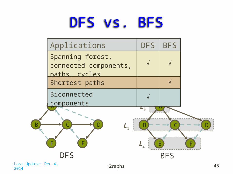
DFS vs. BFS
Graphs 45
CB
A
E
D
F
DFS
CB
A
E
D
L0
L1
FL2
BFS
Applications DFS BFSSpanning forest, connected components, paths, cycles
Shortest paths
Biconnected components
Last Update: Dec 4, 2014

DFS vs. BFS (cont.)Back edge (v,w)– w is an ancestor of v in
the tree of discovery edges
Cross edge (v,w)– w is in the same level as v
or in the next level
Graphs 46
CB
A
E
D
F
DFS
CB
A
E
D
L0
L1
FL2
BFS
Last Update: Dec 4, 2014
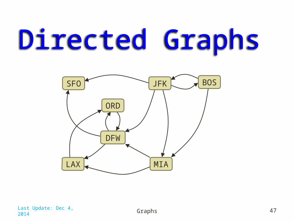
Directed Graphs
Graphs 47Last Update: Dec 4, 2014
BOSJFK
MIA
DFW
SFO
LAX
ORD
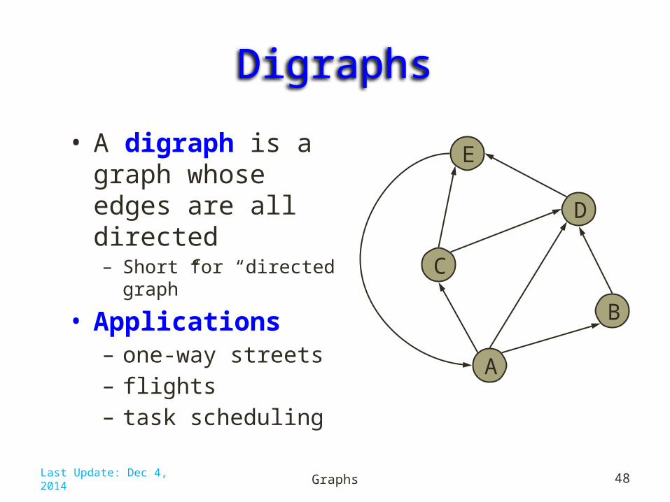
Digraphs• A digraph is a graph
whose edges are all directed– Short for “directed graph”
• Applications– one-way streets– flights– task scheduling
Graphs 48
A
C
E
B
D
Last Update: Dec 4, 2014

Digraph Properties• A graph G=(V,E) such that
Each edge goes in one direction: Edge (a,b) goes from a to b, but not b to a
• If G is simple, m < n(n - 1)• If we keep in-edges and out-edges in separate
adjacency lists, we can perform listing of incoming edges and outgoing edges in time proportional to their size
Graphs 49
A
C
E
B
D
Last Update: Dec 4, 2014

Digraph Application• Scheduling: edge (a,b) means task a must be
completed before task b can be started
Graphs 50
thegoodlife
cs141cs131 cs121
cs53 cs52cs51
cs46cs22cs21
cs161
cs151
cs171
Last Update: Dec 4, 2014
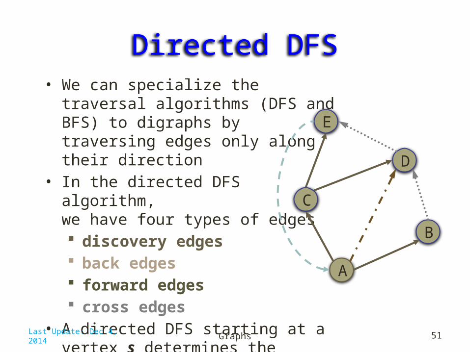
Directed DFS• We can specialize the traversal algorithms
(DFS and BFS) to digraphs by traversing edges only along their direction
• In the directed DFS algorithm, we have four types of edges discovery edges back edges forward edges cross edges
• A directed DFS starting at a vertex s determines the vertices reachable from s
Graphs 51
A
C
E
B
D
Last Update: Dec 4, 2014

Reachability• DFS tree rooted at v:
vertices reachable from v via directed paths
Graphs 52
A
C
E
B
D
FA
C
E D
A
C
E
B
D
F
Last Update: Dec 4, 2014

Strong ConnectivityEach vertex can reach all other vertices
Graphs 53
a
d
c
b
e
f
g
Last Update: Dec 4, 2014

Strong Connectivity Algorithm• For each vertex v in G do:– Perform a DFS from v in G If there’s a w not visited, return “no”
– Let G’ be G with edges reversed– Perform a DFS from v in G’ If there’s a w not visited, return “no”
• Else, return “yes”• Running time: O(n(n+m))
Graphs 54
G:
G’:
a
d
c
b
e
f
g
a
d
c
b
e
f
g
Last Update: Dec 4, 2014
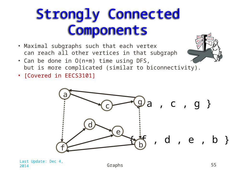
Strongly Connected Components• Maximal subgraphs such that each vertex
can reach all other vertices in that subgraph• Can be done in O(n+m) time using DFS,
but is more complicated (similar to biconnectivity). • [Covered in EECS3101]
Graphs 55
{ a , c , g }
{ f , d , e , b }
a
d
c
b
e
f
g
Last Update: Dec 4, 2014

Transitive ClosureTransitive closure of digraph G is the digraph G* such that
1. G* has the same vertices as G2. G* has a directed edge u v
G has a directed path from u to v (u v)
G* provides reachability information about G
Graphs 56
B
A
D
C
E
G
Last Update: Dec 4, 2014
B
D
C
E
G*
A

If there's a way to get from A to B and fromB to C, then there's a way to get from A to C.
Computing the Transitive Closure• We can perform
DFS starting at each vertex– O(n(n+m))
Graphs 57
Alternatively ... Use dynamic programming: The Floyd-Warshall Algorithm
Last Update: Dec 4, 2014

Floyd-Warshall Transitive Closure• Idea 1: Number the vertices 1, 2, …, n.• Idea 2: Consider paths that use only vertices
numbered 1, 2, …, k, as intermediate vertices:
Graphs 58
k
j
i
Uses only verticesnumbered 1,…,k-1 Uses only vertices
numbered 1,…,k-1
Uses only vertices numbered 1,…,k(add this edge if it’s not already in)
Last Update: Dec 4, 2014

Floyd-Warshall’s Algorithm• Number vertices v1 , …, vn
• Compute digraphs G0 , … , Gn
– G0 = G
– Gk has directed edge (vi , vj) if G has a directed path from vi to vj with intermediate vertices in {v1 , …, vk}
• We have that Gn = G*
• In phase k, digraph Gk is computed from Gk – 1
• Running time: O(n3), assuming areAdjacent is O(1) (e.g., adjacency matrix)
Graphs 59
Algorithm FloydWarshall(G)Input: digraph GOutput: transitive closure G* of G
i 1for all v G.vertices()
denote v as vi
i i + 1G0 Gfor k 1 .. n do
Gk Gk - 1
for i 1 .. n (i k) dofor j 1 .. n (j
i , k) doif Gk – 1 .
areAdjacent(vi, vk)
Gk – 1 . areAdjacent(vk, vj)
if Gk . areAdjacent(vi, vj)
Gk . insertDirectedEdge(vi, vj , k)
return Gn
Last Update: Dec 4, 2014

Java Implementation
Graphs 60Last Update: Dec 4, 2014
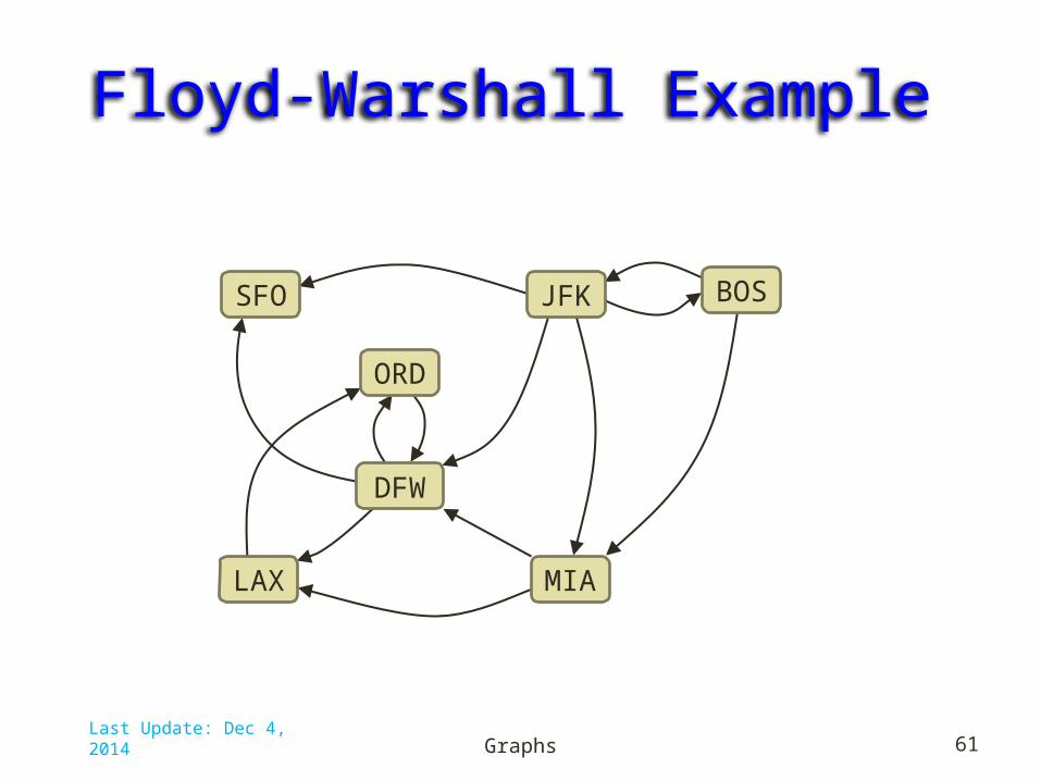
Floyd-Warshall Example
Graphs 61Last Update: Dec 4, 2014
BOSJFK
MIA
DFW
SFO
LAX
ORD

Floyd-Warshall Example
Graphs 62Last Update: Dec 4, 2014
v7v6
v5
v3
v2
v1
v4

Iterataion k = 1
Graphs 63Last Update: Dec 4, 2014
v7v6
v5
v3
v2
v1
v4
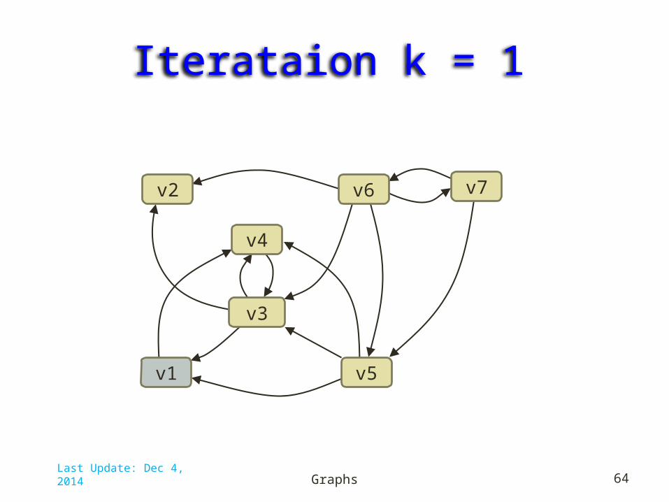
Iterataion k = 1
Graphs 64Last Update: Dec 4, 2014
v7v6
v5
v3
v2
v1
v4

Iterataion k = 2
Graphs 65Last Update: Dec 4, 2014
v7v6
v5
v3
v2
v1
v4
No new edges added
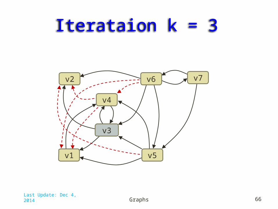
Iterataion k = 3
Graphs 66Last Update: Dec 4, 2014
v3
v7v6
v5
v2
v1
v4

Iterataion k = 3
Graphs 67Last Update: Dec 4, 2014
v3
v1
v7v6v2
v4
v5
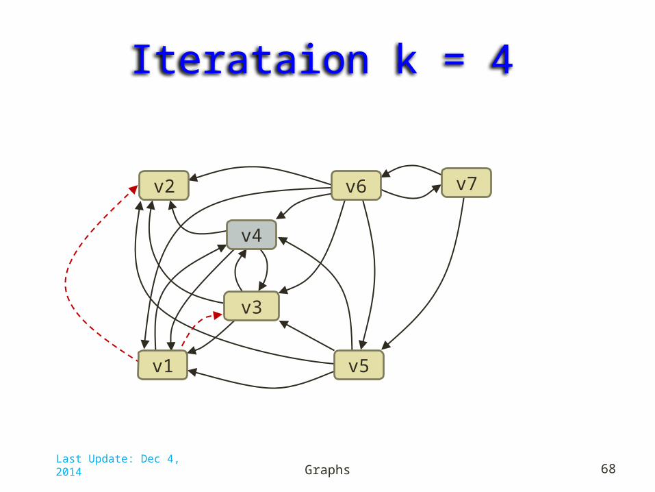
Iterataion k = 4
Graphs 68Last Update: Dec 4, 2014
v3
v7v6v2
v4
v5v1
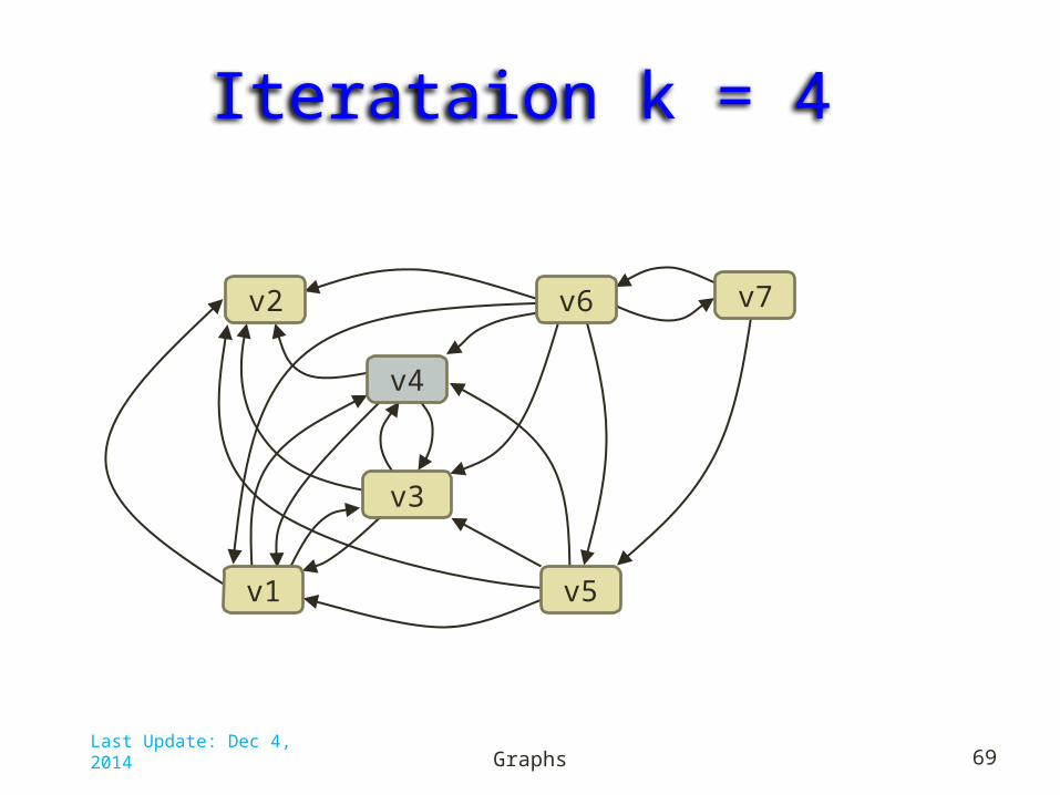
Iterataion k = 4
Graphs 69Last Update: Dec 4, 2014
v3
v7v6v2
v4
v5v1

Iterataion k = 5
Graphs 70Last Update: Dec 4, 2014
v3
v6v2
v4
v5v1
v7

Iterataion k = 5
Graphs 71Last Update: Dec 4, 2014
v3
v6v2
v4
v5v1
v7

Iterataion k = 6
Graphs 72Last Update: Dec 4, 2014
v3
v6v2
v4
v5v1
v7
No new edges added
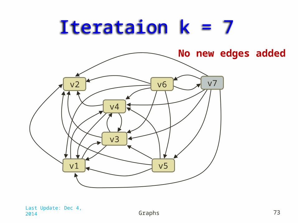
Iterataion k = 7
Graphs 73Last Update: Dec 4, 2014
v3
v6v2
v4
v5v1
v7
No new edges added
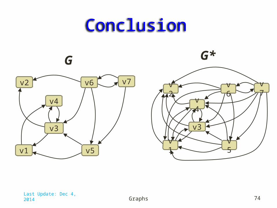
Conclusion
Graphs 74Last Update: Dec 4, 2014
v7v6
v5
v3
v2
v1
v4
G
v3
v6v2
v4
v5v1
v7
G*

DAGs and Topological Ordering• A directed acyclic graph (DAG) is a
digraph that has no directed cycles
• A topological ordering of a digraph is a numbering
v1 , …, vn
of the vertices such that for every edge (vi , vj), we have i < j
• Example: in a task scheduling digraph, a topological ordering of tasks satisfies the precedence constraints
• Theorem:A digraph admits a topological ordering if and only if it is a DAG
Graphs 75
B
A
D
C
E
DAG G
B
A
D
C
E
Topological ordering of Gv1
v2
v3
v4 v5
Last Update: Dec 4, 2014
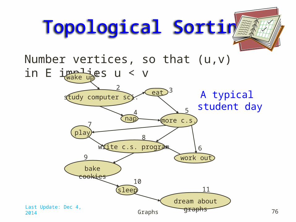
Topological SortingNumber vertices, so that (u,v) in E implies u < v
Graphs 76
write c.s. program
play
wake up
eat
nap
study computer sci.
more c.s.
work out
sleep
dream about graphs
A typical student day
1
2 3
4 5
6
7
8
9
1011
bake cookies
Last Update: Dec 4, 2014
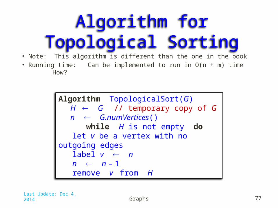
Algorithm for Topological Sorting• Note: This algorithm is different than the one in the book• Running time: Can be implemented to run in O(n + m) time
How?
Graphs 77
Algorithm TopologicalSort(G) H G // temporary copy of G n G.numVertices() while H is not empty do
let v be a vertex with no outgoing edgeslabel v nn n – 1 remove v from H
Last Update: Dec 4, 2014
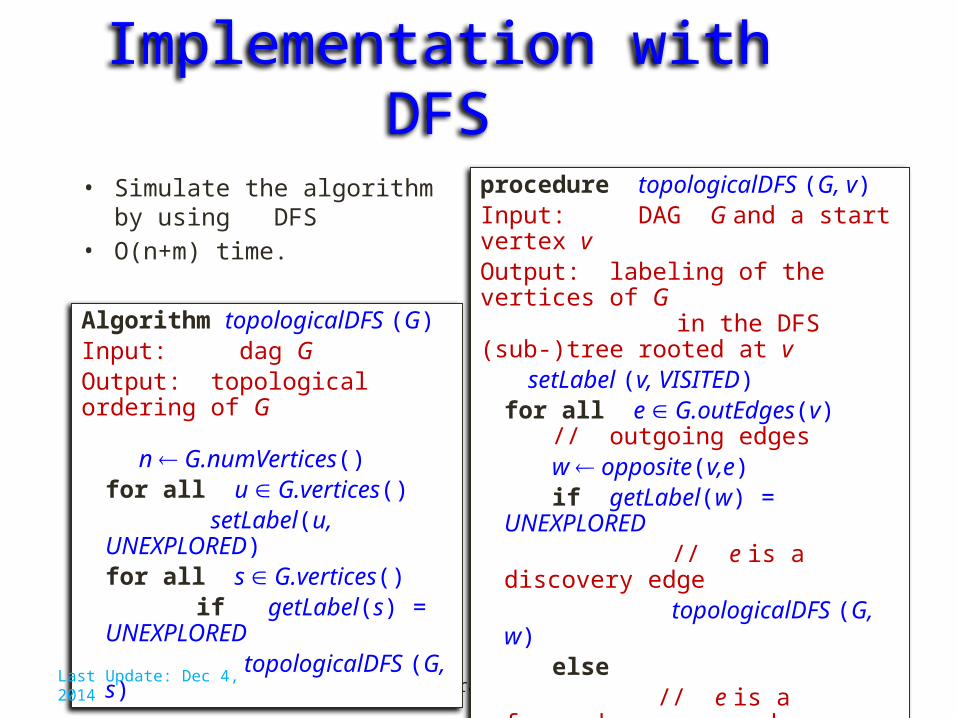
Implementation with DFS• Simulate the algorithm by
using DFS• O(n+m) time.
Graphs 78
procedure topologicalDFS (G, v)Input: DAG G and a start vertex v Output: labeling of the vertices of G
in the DFS (sub-)tree rooted at v
setLabel (v, VISITED)for all e G.outEdges(v)
// outgoing edges w opposite(v,e)if getLabel(w) = UNEXPLORED
// e is a discovery edge
topologicalDFS (G, w)
else // e is a forward
or cross edge Label v with topological number n n n – 1
Algorithm topologicalDFS (G)Input: dag GOutput: topological ordering of G n G.numVertices()
for all u G.vertices() setLabel(u,
UNEXPLORED)for all s G.vertices()
if getLabel(s) = UNEXPLORED
topologicalDFS (G, s)
Last Update: Dec 4, 2014

Topological Sorting Example
Graphs 79Last Update: Dec 4, 2014

Topological Sorting Example
Graphs 80
9Last Update: Dec 4, 2014
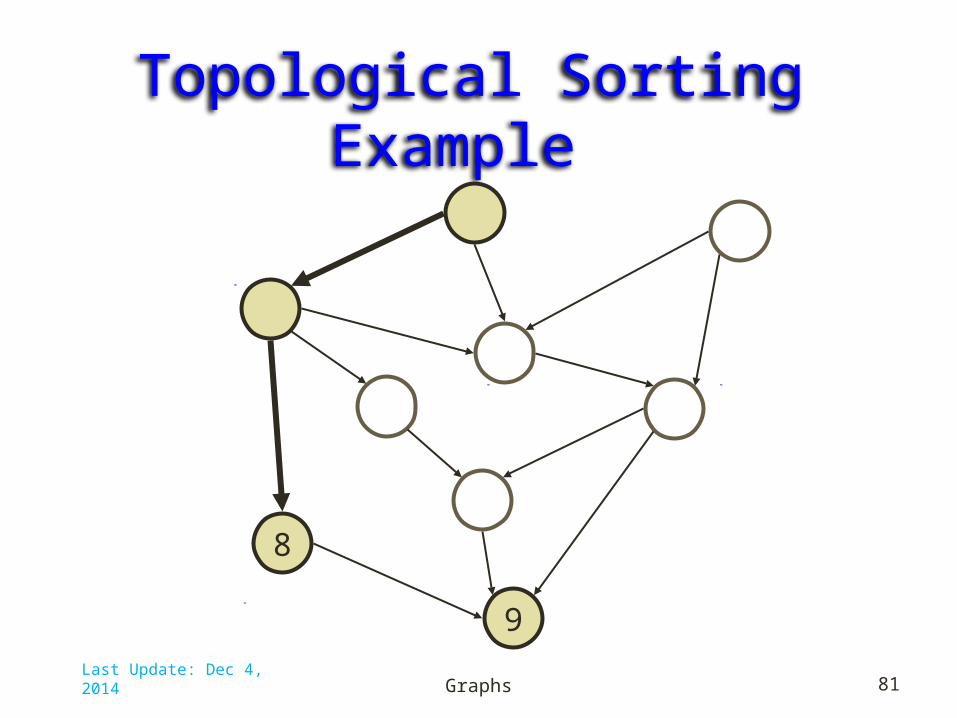
Topological Sorting Example
Graphs 81
8
9Last Update: Dec 4, 2014
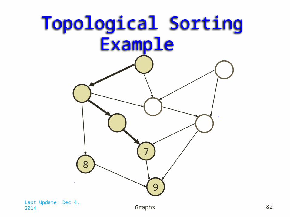
Topological Sorting Example
Graphs 82
78
9Last Update: Dec 4, 2014

Topological Sorting Example
Graphs 83
78
6
9Last Update: Dec 4, 2014
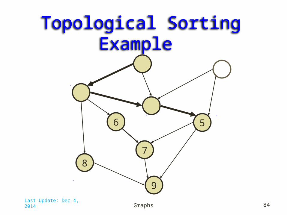
Topological Sorting Example
Graphs 84
78
56
9Last Update: Dec 4, 2014

Topological Sorting Example
Graphs 85
7
4
8
56
9Last Update: Dec 4, 2014

Topological Sorting Example
Graphs 86
7
4
8
56
3
9Last Update: Dec 4, 2014

Topological Sorting Example
Graphs 87
2
7
4
8
56
3
9Last Update: Dec 4, 2014

Topological Sorting Example
Graphs 88
2
7
4
8
56
1
3
9Last Update: Dec 4, 2014
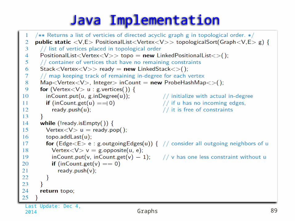
Java Implementation
Graphs 89Last Update: Dec 4, 2014

Shortest Paths
Graphs 90
CB
A
E
D
F
0
328
5 8
48
7 1
2 5
2
3 9
Last Update: Dec 4, 2014

Weighted Graphs• In a weighted graph, each edge has an associated numerical
value, called the weight of the edge• Edge weights may represent, distances, costs, etc.• Example:– In a flight route graph, the weight of an edge represents
the distance in miles between the endpoint airports
Graphs 91
ORD PVD
MIADFW
SFO
LAX
LGA
HNL
849
802
13871743
1843
10991120
1233337
2555
142
12
05
Last Update: Dec 4, 2014

Shortest Paths• Given a weighted graph and two vertices u and v, we want to find a
path of minimum total weight between u and v.– Length of a path is the sum of the weights of its edges.
• Example: Shortest path between Providence and Honolulu• Applications:
– Internet packet routing – Flight reservations– Driving directions
Graphs 92
ORD PVD
MIADFW
SFO
LAX
LGA
HNL
849
802
13871743
1843
10991120
1233337
2555
142
12
05
Last Update: Dec 4, 2014

Shortest Path PropertiesProperty 1: A subpath of a shortest path is itself a shortest pathProperty 2: There is a tree of shortest paths from a start vertex to all
the other vertices
Example: Tree of shortest paths from Providence
Graphs 93
ORD PVD
MIADFW
SFO
LAX
LGA
HNL
849
802
13871743
1843
10991120
1233337
2555
142
12
05
Last Update: Dec 4, 2014

Dijkstra’s Algorithm• The distance from a vertex s to v is the length of a
shortest path from s to v
• Assumptions:– connected & undirected graph– edge weights nonnegative
• Dijkstra’s algorithm computes distances of all vertices from a given start vertex s
Graphs 94Last Update: Dec 4, 2014

Dijkstra’s Algorithm• We grow a “cloud” of vertices, beginning with s and eventually
covering all vertices
• We store with each vertex v a label d(v) representing the distance of v from s in the subgraph consisting of the cloud and its adjacent vertices
• At each step– We add to the cloud the vertex u outside the cloud with
the smallest distance label, d(u)– We update the labels of the vertices adjacent to u
Graphs 95Last Update: Dec 4, 2014
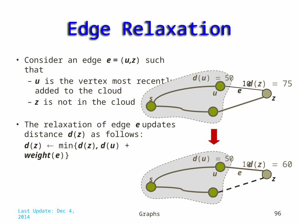
Edge Relaxation• Consider an edge e = (u,z) such that– u is the vertex most recently
added to the cloud– z is not in the cloud
• The relaxation of edge e updates distance d(z) as follows:d(z) min{d(z), d(u) + weight(e)}
Graphs 96
d(z) = 75
d(u) = 5010
zsu e
d(z) = 60
d(u) = 5010
zsu e
Last Update: Dec 4, 2014
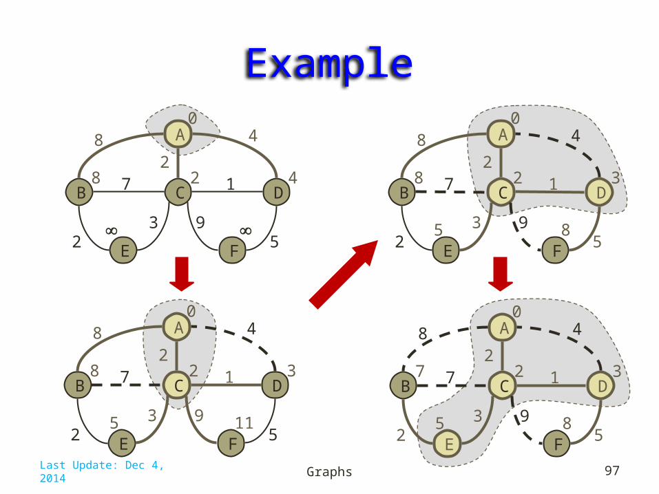
Example
Graphs 97
CB
A
E
D
F
0
428
48
7 1
2 5
2
3 9
CB
A
E
D
F
0
328
5 11
48
7 1
2 5
2
3 9
CB
A
E
D
F
0
328
5 8
48
7 1
2 5
2
3 9
CB
A
E
D
F
0
327
5 8
48
7 1
2 5
2
3 9
Last Update: Dec 4, 2014
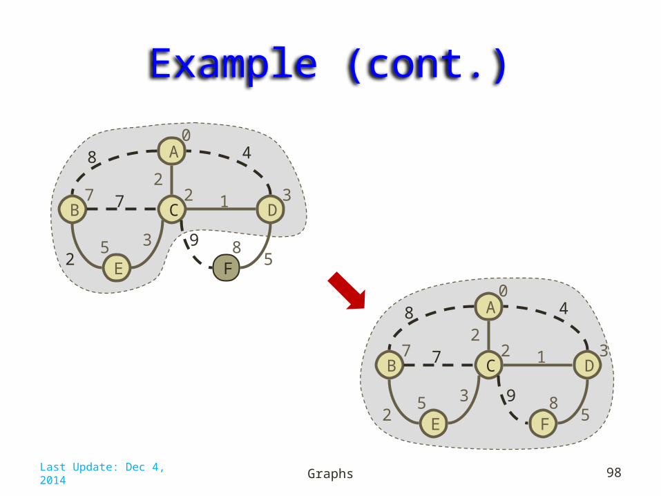
Example (cont.)
Graphs 98
CB
A
E
D
F
0
327
5 8
48
7 1
2 5
2
3 9
CB
A
E
D
F
0
327
5 8
48
7 1
2 5
2
3 9
Last Update: Dec 4, 2014

Dijkstra’s Algorithm
Last Update: Dec 4, 2014 Graphs 99

Analysis of Dijkstra’s Algorithm• Graph operations: We find all the incident edges once for each vertex• Label operations:
– We set/get the distance and locator labels of vertex z O(deg(z)) times– Setting/getting a label takes O(1) time
• Priority queue operations:– Each vertex is inserted/removed once into/from the priority
queue, where each insertion or removal takes O(log n) time– The key of a vertex in the priority queue is modified at most
deg(w) times, where each key change takes O(log n) time
• Dijkstra’s algorithm runs in O((n + m) log n) time provided the graph is represented by the adjacency list/map structure– Recall that v deg(v) = 2m
• So, running time is O(m log n) since the graph is connected
Graphs 100Last Update: Dec 4, 2014
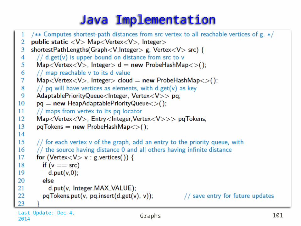
Java Implementation
Graphs 101Last Update: Dec 4, 2014

Java Implementation, 2
Graphs 102Last Update: Dec 4, 2014

Why Dijkstra’s Algorithm WorksDijkstra’s algorithm is based on the greedy method. It adds vertices by increasing distance.
Graphs 103
CB
A
E
D
F
0
327
5 8
48
7 1
2 5
2
3 9
Suppose it didn’t find all shortest distances. Let F be the first wrong vertex the algorithm processed.
When the previous node, D, on the true shortest path was considered, its distance was correct
But the edge (D,F) was relaxed at that time! Thus, so long as d(F) > d(D), F’s distance
cannot be wrong. That is, there is no wrong vertex
Last Update: Dec 4, 2014
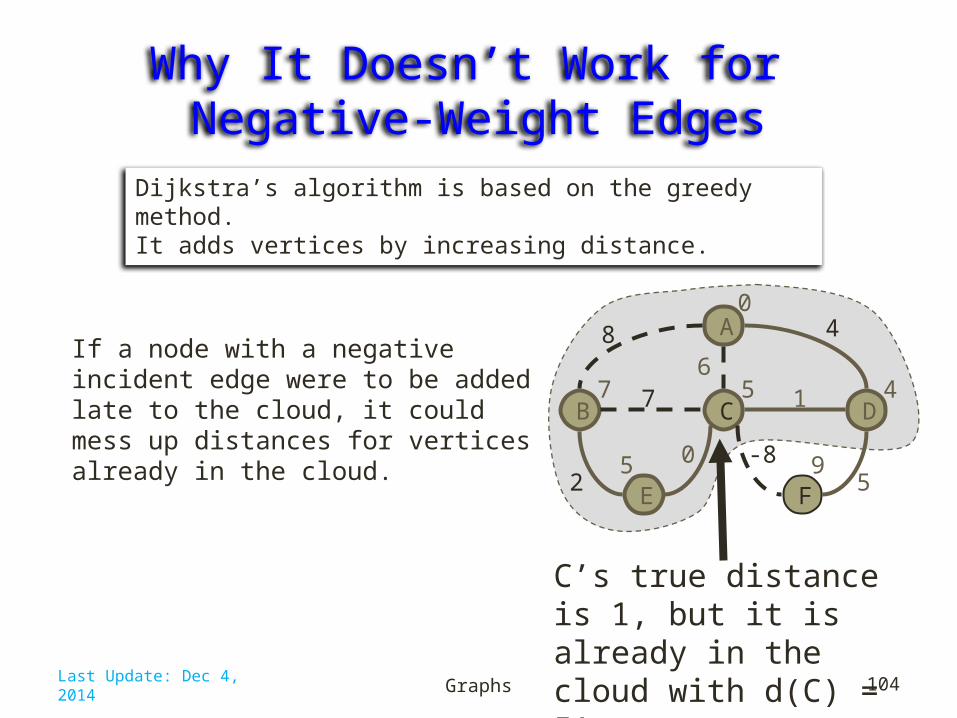
Why It Doesn’t Work for Negative-Weight EdgesIf a node with a negative incident edge were to be added late to the cloud, it could mess up distances for vertices already in the cloud.
Graphs 104
CB
A
E
D
F
0
457
5 9
48
7 1
2 5
6
0 -8
C’s true distance is 1, but it is already in the cloud with d(C) = 5!
Last Update: Dec 4, 2014
Dijkstra’s algorithm is based on the greedy method. It adds vertices by increasing distance.
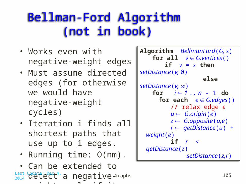
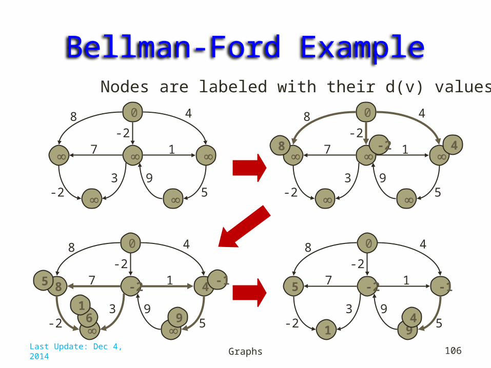
Bellman-Ford Algorithm (not in book)• Works even with negative-
weight edges• Must assume directed edges
(for otherwise we would have negative-weight cycles)
• Iteration i finds all shortest paths that use up to i edges.
• Running time: O(nm).• Can be extended to detect a
negative-weight cycle if it exists – How?
Graphs 105
Algorithm BellmanFord(G, s)for all v G.vertices()
if v = s then setDistance(v, 0)
else setDistance(v, )
for i 1 .. n - 1 dofor each e G.edges()
// relax edge e u G.origin(e)z
G.opposite(u,e)r
getDistance(u) + weight(e)if r <
getDistance(z)
setDistance(z,r)Last Update: Dec 4, 2014
Bellman-Ford Example
Graphs 106
0
48
7 1
-2 5
-2
3 9
Nodes are labeled with their d(v) values
-2
0
48
7 1
-2 53 9
8 -2 4
-2
-28
0
4
48
7 1
-2 53 9
-15
61
9
-25
0
1
-1
9
48
7 1
-2 5
-2
3 94
Last Update: Dec 4, 2014

DAG-based Algorithm (not in book)• Works even with
negative-weight edges• Uses topological order• Does not use any fancy
data structures• Is much faster than
Dijkstra’s algorithm• Running time: O(n+m).
Graphs 107
Algorithm DagDistances(G, s)for all v G.vertices()
if v = s then setDistance(v, 0)
else setDistance(v, )Perform a topological sort of the
verticesfor u 1 .. n do // in topological
orderfor each e G.outEdges(u)
// relax edge e z G.opposite(u,e)r getDistance(u) +
weight(e)if r < getDistance(z)
setDistance(z,r)Last Update: Dec 4, 2014

DAG Example
Graphs 108
Nodes are labeled with their d(v) values
0
48
7 1
-5 5
-2
3 9
1
2 43
6 5
-2
0
48
7 1
-5 53 9
-2 4
1
2 43
6 5
8
-2
-28
0
4
48
7 1
-5 53 9
-1
1 7
1
2 43
6 5
5
6 5
-25
0
1
-1
7
48
7 1
-5 5
-2
3 94
1
2 43
0
(two steps)Last Update: Dec 4, 2014

MinimumSpanning Trees
Graphs 109Last Update: Dec 4, 2014

Minimum Spanning TreesSpanning subgraph
– Subgraph of a graph G containing all the vertices of G
Spanning tree– Spanning subgraph that is itself a
(free) tree
Minimum spanning tree (MST)– Spanning tree of a weighted
graph with minimum total edge weight
• Applications– Communications networks– Transportation networks
Graphs 110
ORD
PIT
ATL
STL
DEN
DFW
DCA
101
9
8
6
3
25
7
4
Last Update: Dec 4, 2014

Cycle PropertyCycle Property:
– Let T be a minimum spanning tree of a weighted graph G
– Let e be an edge of G that is not in T and let C be the cycle formed when e is added to T
– For every edge f of C, weight(f) weight(e)
Proof:– By contradiction– If weight(f) > weight(e) we can get a
spanning tree of smaller weight by replacing e with f
Graphs 111
84
2 36
7
7
9
8e
C
f
84
2 36
7
7
9
8
C
e
f
Replacing f with e yieldsa better spanning tree
Last Update: Dec 4, 2014

Partition PropertyPartition Property:– Consider a partition of the vertices of G into
subsets U and V– Let e be an edge of minimum weight across the
partition– There is a minimum spanning tree of G
containing edge eProof:– Let T be an MST of G– If T does not contain e, consider the cycle C
formed by e+T and let f be an edge of C across the partition
– By the cycle property,weight(f) weight(e)
– Thus, weight(f) = weight(e)– We obtain another MST by replacing f with e
Graphs 112
U V
74
2 85
7
3
9
8 e
f
74
2 85
7
3
9
8 e
f
Replacing f with e yieldsanother MST
U V
Last Update: Dec 4, 2014

Prim-Jarnik’s Algorithm• Similar to Dijkstra’s algorithm• We pick an arbitrary vertex s and we grow the MST as a cloud of
vertices, starting from s• We store with each vertex v label d(v) representing the smallest
weight of an edge connecting v to a vertex in the cloud • At each step:– We add to the cloud the vertex u outside the cloud with the
smallest distance label– We update the labels of the vertices adjacent to u
Graphs 113Last Update: Dec 4, 2014
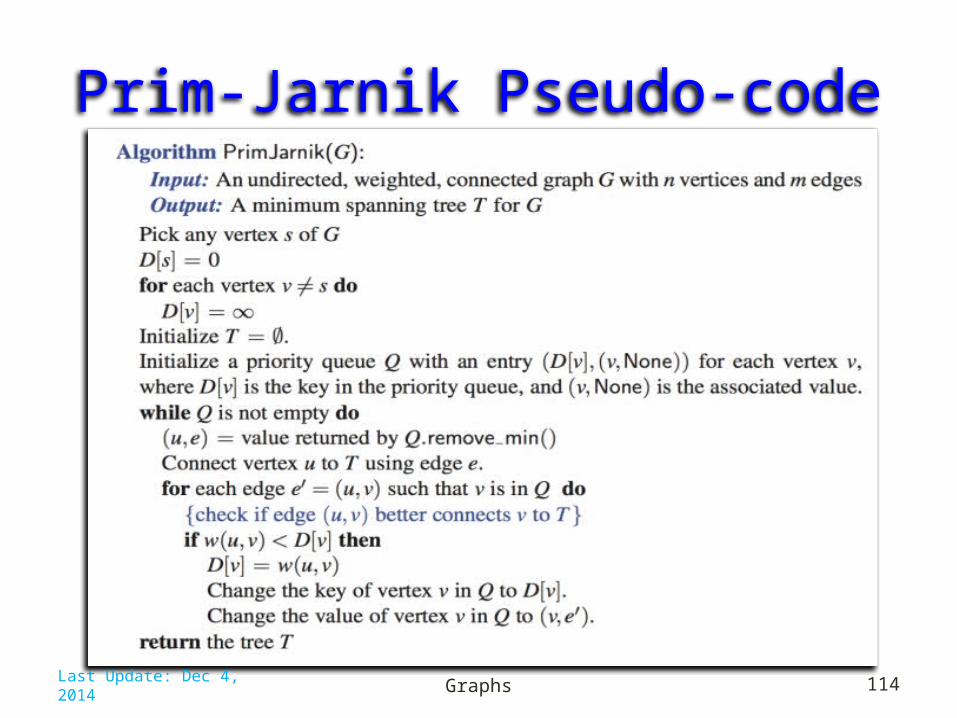
Prim-Jarnik Pseudo-code
Graphs 114Last Update: Dec 4, 2014
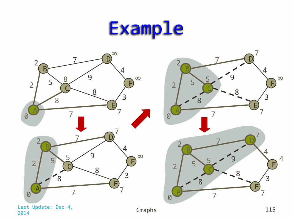
Example
Graphs 115
BD
C
A
F
E
74
28
5
7
3
9
8
07
2
8
BD
C
A
F
E
74
28
5
7
3
9
8
07
2
5 4
7
BD
C
A
F
E
74
28
5
7
3
9
8
07
2
5
7
BD
C
A
F
E
74
28
5
7
3
9
8
07
2
5
7
Last Update: Dec 4, 2014
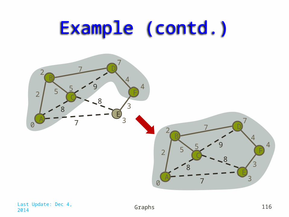
Example (contd.)
Graphs 116
BD
C
A
F
E
74
28
5
7
3
9
8
03
2
5 4
7
BD
C
A
F
E
74
28
5
7
3
9
8
03
2
5 4
7
Last Update: Dec 4, 2014

Analysis• Graph operations
– We cycle through the incident edges once for each vertex• Label operations
– We set/get the distance, parent and locator labels of vertex z O(deg(z)) times– Setting/getting a label takes O(1) time
• Priority queue operations– Each vertex is inserted once into and removed once from the priority queue,
where each insertion or removal takes O(log n) time– The key of a vertex w in the priority queue is modified at most deg(w) times,
where each key change takes O(log n) time • Prim-Jarnik’s algorithm runs in O((n + m) log n) time provided the graph is
represented by the adjacency list structure– Recall that v deg(v) = 2m
• The running time is O(m log n) since the graph is connected
Graphs 117Last Update: Dec 4, 2014
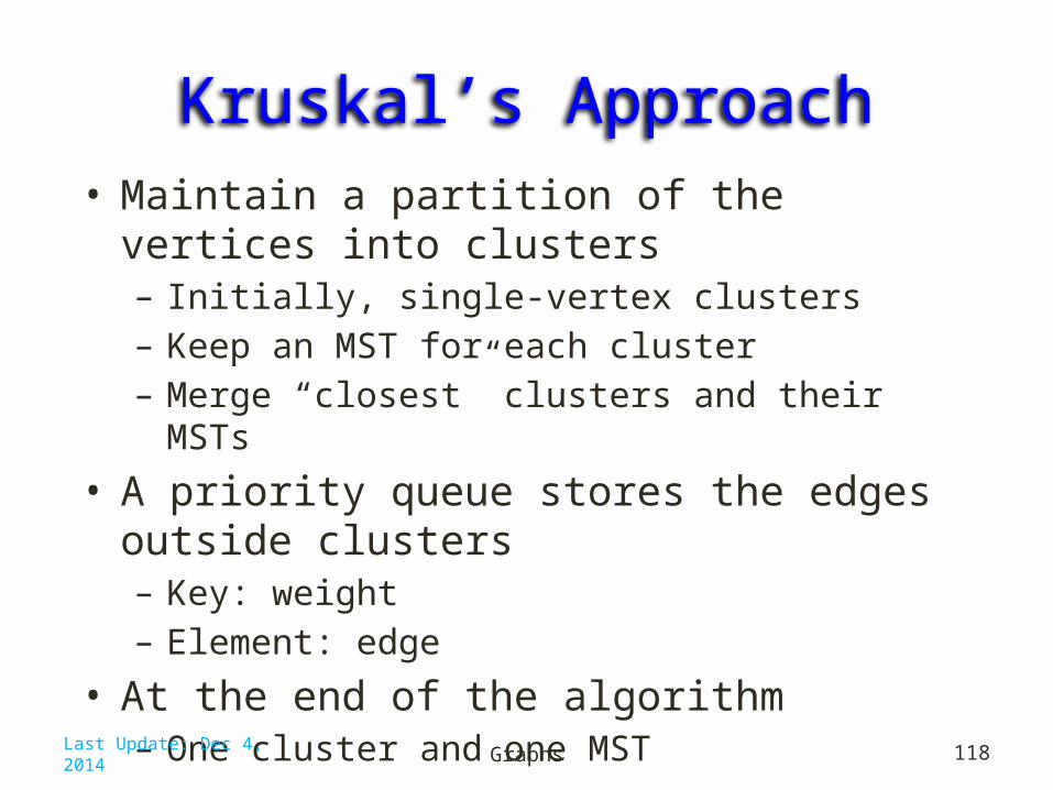
Kruskal’s Approach• Maintain a partition of the vertices into clusters– Initially, single-vertex clusters– Keep an MST for each cluster– Merge “closest” clusters and their MSTs
• A priority queue stores the edges outside clusters– Key: weight– Element: edge
• At the end of the algorithm– One cluster and one MST
Graphs 118Last Update: Dec 4, 2014

Kruskal’s Algorithm
Graphs 119Last Update: Dec 4, 2014

Example
Graphs 120Last Update: Dec 4, 2014
BG
C
A
F
D
4
1 35
10
2
8
7
6E
H11
9
7
BG
C
A
F
D
4
1 35
10
2
8
7
6E
H11
9
7
BG
C
A
F
D
4
1 35
10
2
8
7
6E
H11
9
7
BG
C
A
F
D
4
1 35
10
2
8
7
6E
H11
9
7

Example (contd.)
Graphs 121Last Update: Dec 4, 2014
BG
C
A
F
D
4
1 35
10
2
8
7
6E
H11
9
7
BG
C
A
F
D
4
1 35
10
2
8
7
6E
H11
9
7 3 st
eps
BG
C
A
F
D
4
1 35
10
2
8
7
6E
H11
9
7
4 steps
BG
C
A
F
D
4
1 35
10
2
8
7
6E
H11
9
7

Data Structure for Kruskal’s Algorithm• The algorithm maintains a forest of trees
• A priority queue extracts the edges by increasing weight
• An edge is accepted if it connects distinct trees
• We need a data structure that maintains a partition, i.e., a collection of disjoint sets, with operations: makeSet(u): create a set consisting of u find(u): return the set storing u union(A, B): replace sets A and B with their union
Graphs 122Last Update: Dec 4, 2014

List-based Partition
Graphs 123Last Update: Dec 4, 2014
• Each set is stored in a sequence• Each element has a reference back to the set– operation find(u) takes O(1) time, and returns the set
of which u is a member.– in operation union(A,B), we move the elements of
the smaller set to the sequence of the larger set and update their references
– the time for operation union(A,B) is min(|A|, |B|)
• Whenever an element is processed, it goes into a set of size at least double, hence each element is processed at most log n times
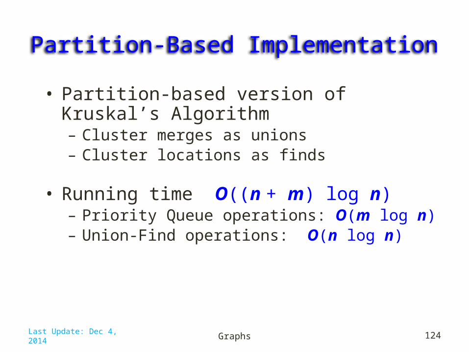
Partition-Based Implementation• Partition-based version of Kruskal’s Algorithm – Cluster merges as unions – Cluster locations as finds
• Running time O((n + m) log n)– Priority Queue operations: O(m log n)– Union-Find operations: O(n log n)
Graphs 124Last Update: Dec 4, 2014

Java Implementation
Graphs 125Last Update: Dec 4, 2014
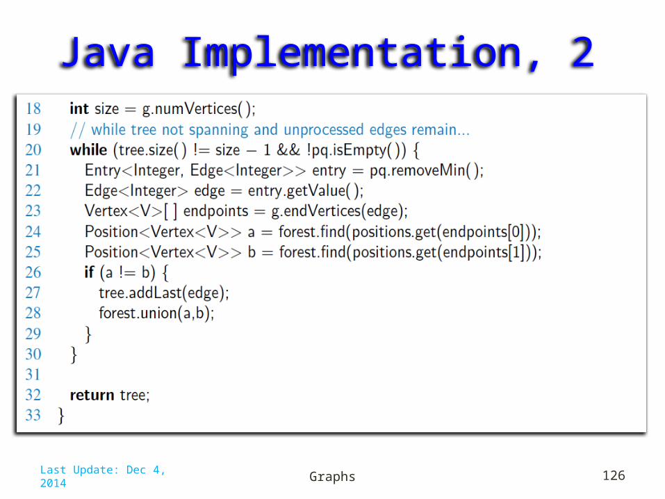
Java Implementation, 2
Graphs 126Last Update: Dec 4, 2014

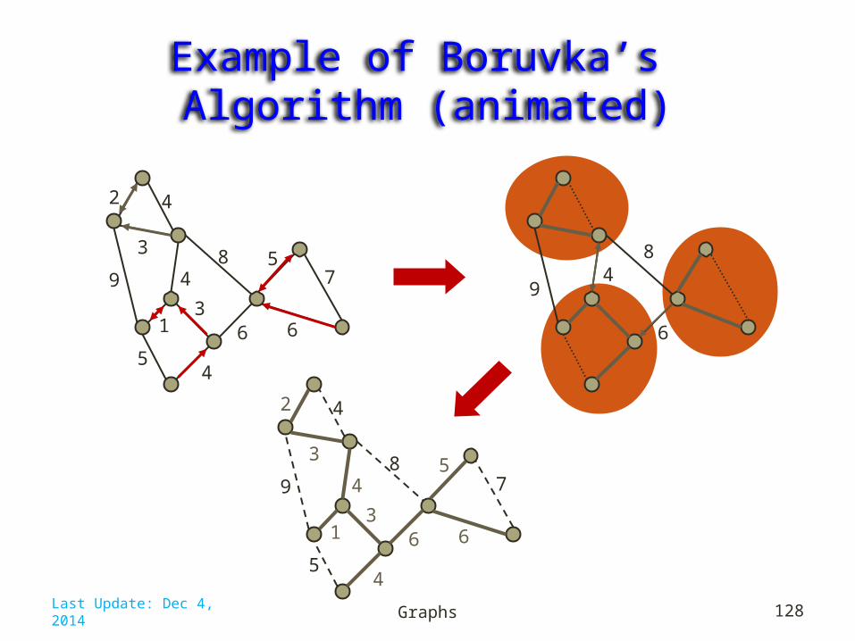
Boruvka’s Algorithm (Exercise)• Like Kruskal’s Algorithm, Boruvka’s algorithm grows many clusters at
once and maintains a forest T• Each iteration of the while loop halves the number of connected
components in forest T• The running time is O(m log n)
Graphs 127
Algorithm BoruvkaMST(G)T V // just the vertices of Gwhile T has fewer than n – 1 edges do
for each connected component C in T do
Let edge e be the smallest-weight edge from C
to another component in T
if e is not already in T then Add edge e to T
return T
Last Update: Dec 4, 2014
Example of Boruvka’s Algorithm (animated)
Graphs 128
1
54
3
2
3
4
49
6
87
6
54
9
6
8
1
54
3
2
3
4
49
6
87
6
5
Last Update: Dec 4, 2014

Union-Find Partition Structures
Graphs 129Last Update: Dec 4, 2014

Partitions with Union-Find OperationsmakeSet(x): Create a singleton set containing
the element x and return the position storing x in this set
union(A,B ): Return the set A U B, destroying the old A and B
find(p): Return the set containing the element at position p
Graphs 130Last Update: Dec 4, 2014

List-based Implementation• Each set is stored in a sequence represented with
a linked-list• Each node should store an object containing the
element and a reference to the set name
Graphs 131Last Update: Dec 4, 2014

Analysis of List-based Representation• When doing a union, always move elements
from the smaller set to the larger set Each time an element is moved it goes to a set of
size at least double its old set Thus, an element can be moved at most O(log n)
times• Total time needed to do n unions and finds is
O(n log n).
Graphs 132Last Update: Dec 4, 2014

Tree-based Implementation• Each element is stored in a node, which contains a pointer
to a set name• A node v whose set pointer points back to v is also a set
name• Each set is a tree, rooted at a node with a self-referencing
set pointer• Example: The sets “1”, “2”, and “5”:
Graphs 133
1
74
2
63
5
108
12
119
Last Update: Dec 4, 2014

Union-Find Operations• To do a union, simply make
the root of one tree point to the root of the other
• To do a find, follow set-name pointers from the starting node until reaching a node whose set-name pointer refers back to itself
Graphs 134
2
63
5
108
12
11
9
2
63
5
108
12
11
9
Last Update: Dec 4, 2014
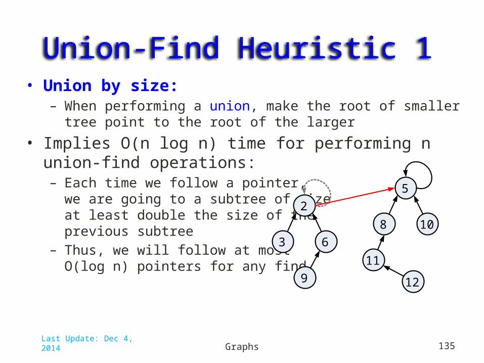
Union-Find Heuristic 1• Union by size:
– When performing a union, make the root of smaller tree point to the root of the larger
• Implies O(n log n) time for performing n union-find operations:– Each time we follow a pointer,
we are going to a subtree of size at least double the size of the previous subtree
– Thus, we will follow at most O(log n) pointers for any find.
Graphs 135
2
63
5
108
12
11
9
Last Update: Dec 4, 2014

Union-Find Heuristic 2• Path compression:
– After performing a find, compress all the pointers on the path just traversed so that they all point to the root
• Implies O(n log* n) time for performing n union-find operations:– [Proof is somewhat involved and is covered in EECS 4101]
Graphs 136
2
63
5
108
12
11
9
2
63
5
108
12
11
9
Last Update: Dec 4, 2014
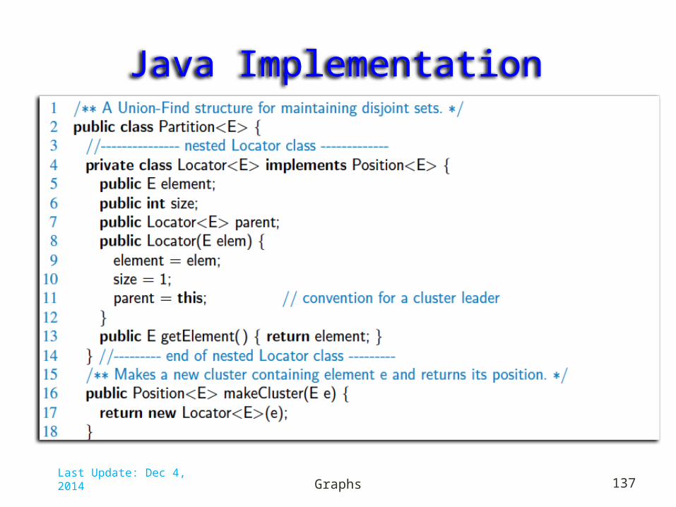
Java Implementation
Graphs 137Last Update: Dec 4, 2014
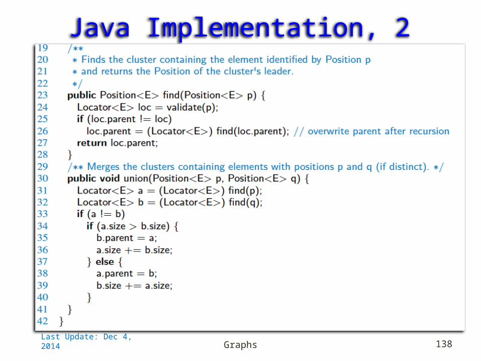
Java Implementation, 2
Graphs 138Last Update: Dec 4, 2014

Summary
Last Update: Dec 4, 2014 Graphs 139
• Graph terminology & representation data structures• Graph Traversals:– Depth First Search– Breadth First Search
• Transitive Closure: Floyd-Warshall• Topological Sorting of DAGs• Shortest Paths in Weighted graphs– Dijkstra, Bellman-Ford, DAGs
• Minimum Spanning Trees– Prim-Jarnik, Boruvka, Kruskal
• Disjoint Partitions & Union-Find Structures

Last Update: Dec 4, 2014 Graphs 140