Graphlet decomposition: framework, algorithms, and ... · Recursive decomposition of networks is a...
34
Knowl Inf Syst (2017) 50:689–722 DOI 10.1007/s10115-016-0965-5 REGULAR PAPER Graphlet decomposition: framework, algorithms, and applications Nesreen K. Ahmed 1 · Jennifer Neville 2 · Ryan A. Rossi 3 · Nick G. Duffield 4 · Theodore L. Willke 1 Received: 14 November 2015 / Revised: 5 March 2016 / Accepted: 4 June 2016 / Published online: 27 June 2016 © Springer-Verlag London 2016 Abstract From social science to biology, numerous applications often rely on graphlets for intuitive and meaningful characterization of networks. While graphlets have witnessed a tremendous success and impact in a variety of domains, there has yet to be a fast and efficient framework for computing the frequencies of these subgraph patterns. However, existing methods are not scalable to large networks with billions of nodes and edges. In this paper, we propose a fast, efficient, and parallel framework as well as a family of algorithms for counting k -node graphlets. The proposed framework leverages a number of theoretical combinatorial arguments that allow us to obtain significant improvement on the scalability of graphlet counting. For each edge, we count a few graphlets and obtain the exact counts of others in constant time using the combinatorial arguments. On a large collection of 300+ networks from a variety of domains, our graphlet counting strategies are on average 460× faster than existing methods. This brings new opportunities to investigate the use of graphlets on much larger networks and newer applications as we show in the experiments. To the best of our knowledge, this paper provides the largest graphlet computations to date. Keywords Graphlet · Motif · Graph mining · Graph kernel · Classification · Graph features · Higher-order graph statistics · Biological networks · Visual graph analytics B Nesreen K. Ahmed [email protected] 1 Parallel Computing Lab, Intel Corporation, Santa Clara, CA 95054, USA 2 Department of Computer Science, Purdue University, West Lafayette, IN 47906, USA 3 Palo Alto Research Center (PARC), Palo Alto, CA 94304, USA 4 Department of Electrical and Computer Engineering, Texas A&M University, College Station, TX 77843, USA 123
Transcript of Graphlet decomposition: framework, algorithms, and ... · Recursive decomposition of networks is a...

Knowl Inf Syst (2017) 50:689–722DOI 10.1007/s10115-016-0965-5
REGULAR PAPER
Graphlet decomposition: framework, algorithms,and applications
Nesreen K. Ahmed1 · Jennifer Neville2 ·Ryan A. Rossi3 · Nick G. Duffield4 · Theodore L. Willke1
Received: 14 November 2015 / Revised: 5 March 2016 / Accepted: 4 June 2016 /Published online: 27 June 2016© Springer-Verlag London 2016
Abstract From social science to biology, numerous applications often rely on graphletsfor intuitive and meaningful characterization of networks. While graphlets have witnesseda tremendous success and impact in a variety of domains, there has yet to be a fast andefficient framework for computing the frequencies of these subgraph patterns. However,existing methods are not scalable to large networks with billions of nodes and edges. In thispaper, we propose a fast, efficient, and parallel framework as well as a family of algorithmsfor counting k-node graphlets. The proposed framework leverages a number of theoreticalcombinatorial arguments that allow us to obtain significant improvement on the scalabilityof graphlet counting. For each edge, we count a few graphlets and obtain the exact countsof others in constant time using the combinatorial arguments. On a large collection of 300+networks from a variety of domains, our graphlet counting strategies are on average 460×faster than existing methods. This brings new opportunities to investigate the use of graphletson much larger networks and newer applications as we show in the experiments. To the bestof our knowledge, this paper provides the largest graphlet computations to date.
Keywords Graphlet ·Motif ·Graph mining ·Graph kernel · Classification ·Graph features ·Higher-order graph statistics · Biological networks · Visual graph analytics
B Nesreen K. [email protected]
1 Parallel Computing Lab, Intel Corporation, Santa Clara, CA 95054, USA
2 Department of Computer Science, Purdue University, West Lafayette, IN 47906, USA
3 Palo Alto Research Center (PARC), Palo Alto, CA 94304, USA
4 Department of Electrical and Computer Engineering, Texas A&M University,College Station, TX 77843, USA
123

690 N. K. Ahmed et al.
1 Introduction
Recursive decomposition of networks is a widely used approach in network analysis tofactorize the complex structure of real-world networks into small subgraph patterns of sizek nodes. These patterns are called graphlets [33]. Graphlets (also known as motifs [31])are defined as subgraph patterns recurring in real-world networks at frequencies that arestatistically significant from those in random networks. Given a network, we can count thenumber of embedding of each graphlet in the network, creating a profile of sufficient statisticsthat characterizes the network structure [40].While knowing the graphlet frequencies does notuniquely define the network structure, it has been shown that graphlet frequencies often carrysignificant information about the local network structure in a variety of domains [10,12,21].This is in contrast to global topological properties (e.g. , diameter, degree distribution), wherenetworks with similar/exact global topological properties can exhibit significantly differentlocal structures.
1.1 Graphlets, scalability, and applications
From social science to biology, graphlets have found numerous applications and were usedas the building blocks of network analysis [31]. In social science, graphlet analysis (typicallyknown as k-subgraph census) is widely adopted in sociometric studies [12,21]. Much of thework in this vein focused on analyzing triadic tendencies as important structural features ofsocial networks (e.g. , transitivity or triadic closure) as well as analyzing triadic configura-tions as the basis for various social network theories (e.g. , social balance, strength of weakties, stability of ties, or trust [16]). In biology [29,33], graphlets were widely used for proteinfunction prediction [40], network alignment [30], and phylogeny [25] to name a few. Morerecently, there has been an increased interest in exploring the role of graphlet analysis incomputer networking [7,11,18] (e.g. , for web spam detection, analysis of peer-to-peer pro-tocols and Internet AS graphs), chemoinformatics [22,34], image segmentation [49], amongothers [48].
While graphlet counting and discovery have witnessed a tremendous success and impactin a variety of domains from social science to biology, there has yet to be a fast andefficient approach for computing the frequencies of these patterns. For instance, Sher-vashidze et al. [40] take hours to count graphlets on relatively small biological networks(i.e. , few hundreds/thousands of nodes/edges) and use such counts as features for graph clas-sification [45]. Previous work showed that graphlet counting is computationally intensivesince the number of possible k-subgraphs in a graph G increases exponentially with k inO(|V |k) and can be computed in O(|V |.�k−1) for any bounded degree graph, where � isthe maximum degree of the graph [40].
To address these problems,wepropose a fast, efficient, and parallel framework and a familyof algorithms for counting graphlets of size k = {3, 4}-nodes that take only a fraction of thetime to computewhen compared to the currentmethods used. The proposed graphlet countingalgorithm leverages a number of theoretical combinatorial arguments for different graphlets.For each edge, we count a few graphlets, and with these counts along with the combinatorialarguments, we obtain the exact counts of others in constant time. On a large collection of300+ networks from a variety of domains, our graphlet counting strategies are on average460× faster than the current methods. This brings new opportunities to investigate the use ofgraphlets on much larger networks and newer applications as we show in our experiments.
123

Graphlet decomposition: framework, algorithms, and applications 691
To the best of our knowledge, this paper provides the largest graphlet computations to dateas well as the largest systematic investigation on over 300+ networks.
Furthermore, a number of important machine learning tasks are likely to benefit fromsuch an approach, including graph anomaly detection [32,36], as well as using graphlets asfeatures for improving community detection [39], role discovery [38], graph classification[45], and relational learning [13,37].
We test the scalability of our proposed approach experimentally on 300+ networks froma variety of domains, such as biological, social, and technological domains. We compareour approach to the state-of-the-art exact counting methods such as RAGE [27], FANMOD[47], and Orca [20]. We found that RAGE [27] took 2400s to count graphlets on a small 26knode graph, whereas our proposed method is 460× faster on average, taking only 0.01 s. Wealso note that FANMOD [47], another recent approach, takes 172,800s and Orca [20] takes2.5 s for the same small graph. Our exact graphlet analysis is well suited for shared-memorymulti-core architectures, distributed architectures (MPI), and hybrid implementations thatleverage the advantages of both.
1.2 Contributions
• Algorithms and theoretical analysis: A fast, efficient, and parallel graphlet countingframework and a family of algorithms for graphlet counting. In addition, we provide atheoretical analysis of a number of combinatorial arguments that enable our proposedframework to obtain significant improvement on the scalability of graphlet counting.
• Scalability: The proposed graphlet counting algorithm is on average 460× faster thanthe state-of-the-art methods. In addition, we analyze graphlet counts on graphs of sizesthat are beyond the scope of the state of the art (e.g. , on graphs with billions of nodesand edges).
• Effectiveness: Largest graphlet computations to date and largest systematic evaluationon over 300+ large-scale networks from a variety of domains.
• Applications: Systematic investigation across a variety of existing and new applicationsfor graphlet counting, such as finding unique patterns in graphs, graph similarity, andgraph classification.
2 Background
Graphlets are subgraph patterns recurring in real-world networks at frequencies that aresignificantly higher than those in random networks [31,33]. Previous work showed thatgraphlets can be used to define universal classes of networks [31]. Moreover, graphlets areat the heart and foundation of many network analysis tasks (e.g. , network classification,network alignment) [19,29,33]. In this paper, we introduce an efficient algorithm to computethe number of embedding of each graphlet of size k = {2, 3, 4} nodes in the network (seeTable 1 for notation).
2.1 Notation and definitions
Given an undirected simple input graph G = (V, E), a graphlet of size k nodes is defined asany subgraph Gk ⊂ G which consists of a subset of k nodes of the graph G. In this paper,
123

692 N. K. Ahmed et al.
Table 1 Summary of graphlet notation
Graphlet Description Complement d r |T | K χ D B |C |(k = 4)−Graphlets
Connected
g41 4-Clique 1.00 3 3.0 1.00 4 3 4 1 0 1
g42 4-Chordalcycle 0.83 3 2.5 –0.66 2 2 3 2 1 1
g43 4-Tailedtriangle 0.67 3 2.0 –0.71 1 2 3 2 2 1
g44 4-Cycle 0.67 2 2.0 1.00 0 2 2 2 1 1
g45 3-Star 0.50 3 1.5 –1.00 0 1 2 2 3 1
g46 4-Path 0.50 2 1.5 –0.50 0 1 2 3 2 1
Disconnected
g47 4-Node-1-triangle 0.50 2 1.5 1.00 1 2 3 1 0 2
g48 4-Node-2-star 0.33 2 1.0 –1.00 0 1 2 2 1 2
g49 4-Node-2-edge 0.33 1 1.0 1.00 0 1 2 1 0 2
g410 4-Node-1-edge 0.17 1 0.5 1.00 0 1 2 1 0 3
g411 4-Node-independent 0.00 0 0.0 0.00 0 0 1 ∞ 0 4
(k = 3)−Graphlets
g31 Triangle 1.00 2 2.0 1.00 1 2 3 1 0 1
g32 2-Star 0.67 2 1.33 –1.00 0 1 2 2 1 1
g33 3-Node-1-edge 0.33 1 0.67 1.00 0 1 2 1 0 2
g34 3-Node-independent 0.00 0 0.00 0.00 0 0 1 ∞ 0 3
(k = 2)−Graphlets
g21 Edge 1.00 1 1.0 1.00 0 1 2 1 0 1
g22 2-Node-independent 0.00 0 0.0 0.00 0 0 1 ∞ 0 2
Summary of the notation and properties for the graphlets of size k = {2, 3, 4}. Note that ρ denotes density, and d denotethe max and mean degree, whereas assortativity is denoted by r . Also, |T | denotes the total number of triangles, K is the maxk-core number, χ denotes the Chromatic number, whereas D denotes the diameter, B denotes the max betweenness, and |C |denotes the number of components. Note that if |C | > 1, then r , D, and B are from the largest component.
we mainly focus on computing the frequencies of induced graphlets. An induced graphletis an induced subgraph that consists of all edges between its nodes that are present in theinput graph (as described in Definition 1). In addition, we distinguish between connectedand disconnected graphlets (see Table 1). A graphlet is connected if there is a path from anynode to any other node in the graphlet (see Definition 2). Table 1 provides a summary of thenotation and properties of all possible induced graphlets of size k = {2, 3, 4}.Definition 1 Induced Graphlet: an induced graphlet Gk = (Vk, Ek) is a subgraph that con-sists of a subset of k vertices of the graph G = (V, E) (i.e., Vk ⊂ V ) together with all theedges whose endpoints both are in this subset (i.e. , Ek = {∀e ∈ E | e = (u, v)∧u, v ∈ Vk}).Definition 2 Connected Graphlet: a graphlet Gk = (Vk, Ek) is connected when thereis a path from any node to any other node in the graphlet (i.e. , ∀u, v ∈ Vk,∃Pu−v :u, . . . , w, . . . , v, such that d(u, v) ≥ 0 ∧ d(u, v) = ∞, where d(u, v) is the distancebetween u and v). Assume |C | denotes the number of connected components in a graphletGk . By definition, there exists one and only one connected component in a graphlet Gk (i.e. ,|C | = 1) if and only if Gk is connected.
123

Graphlet decomposition: framework, algorithms, and applications 693
Problem Definition. Given a family of graphlets of size k nodes Gk = {gk1 , gk2 , . . . ,
gkm }, our goal is to count the number of embeddings (appearances) of each graphletgki ∈ Gk in the input graph G. In other words, we need to count the number of inducedgraphlets Gk in G that are isomorphic to each graphlet gki ∈ Gk in the family; such a
number is denoted by
(Ggki
)[17].
A graphlet gki ∈ Gk is embedded in the graph G, if and only if there is an injectivemapping σ : Vgki
→ V , with e = (u, v) ∈ Egkiif and only if e′ = (σ (u), σ (v)) ∈ E .
Table 1 shows that |Gk | = {2, 4, 11} when k = {2, 3, 4}, respectively. Further, given a familyGk = {gk1 , gk2 , . . . , gkm } of graphlets of size k nodes, we define f (gki , G) as the frequencyof any graphlet gki ∈ Gk in the input graph G.
2.2 Relationship to graph complement
The complement of a graph G, denoted by G, is the graph defined on the same vertices as Gsuch that two vertices are connected in G if and only if they are not connected in G. Therefore,the graph sum G + G gives the complete graph on the set of vertices of G. There are directrelationships between the frequencies of graphlets and the frequencies of their complement.For each graphlet gki , there exists a non-isomorphic complementary graphlet pattern gki suchthat two vertices are connected in gki if and only if they are not connected in gki [17]. Forexample, cliques and independent sets of size k nodes are pairs of complementary graphlets.Similarly, chordal cycles of size 4 nodes are complementary to the 4-node-1-edge graphlet(see Table 1). It is also worth noting that the 4-path graphlet is a self-complementary pattern,whichmeans the 4-path is isomorphic to itself. From this discussion, it is clear that the numberof embeddings of each graphlet gki ∈ Gk in the input graph G is equivalent to the number ofembeddings of its complementary graphlet gki in the complement graph G. In other words,f (gki , G) = f (gki , G) [17].
2.3 Relationship to graph/matrix reconstruction theorems
The graph reconstruction conjecture [17] states that an undirected graph G can be uniquelydetermined up to an isomorphism, from the set of all possible vertex-deleted subgraphs of G(i.e. , {Gv}v∈V ) [28]. Verification of this conjecture for all possible graphs up to 6 vertices wascarried by Kelly [23] and later was extended to up to 11 vertices by McKay [28]. Clearly, iftwo graphs are isomorphic (i.e. , G ∼= G ′), then their graphlet frequencies would be the same(i.e. , fk(G) = fk(G ′)), but the reverse remains a converse for the general case of graphs.In contrast, the matrix reconstruction theorem has been resolved [26], which states that anyN × N matrix can be reconstructed from its list of all possible principal minors obtained bythe deletion of the kth row and the kth column [26], which is the foundation of a class ofgraph kernels called the graphlet kernel [40].
2.4 Related work
In this section, we briefly discuss some of the relatedwork, highlighting various graphminingand machine learning tasks that would benefit from our approach. Much of the previous work
123

694 N. K. Ahmed et al.
focused on counting certain types of graphlets (e.g. , only connected graphlets such as cliquesand cycles) [20,24,47]. However, a number of graph mining and machine learning tasks relyon counting all graphlets of a certain size.
For example, some previous work used the full spectrum of graphlet frequencies to definea domain-independent coordinate system in which collections of graphs can be compactlyrepresented and analyzed within a common space [44]. Moreover, a variety of graph kernelshave been proposed in machine learning (e.g. , graphlet, subtree, and random walk kernels)[9,40,45] to bridge the gap between graph learning and kernel methods. And some types ofthe graph kernels, in particular the graphlet kernel, rely on counting all graphlets. However,a general limitation of most graph kernels (including the graphlet kernel) is that they scalepoorly to graphs with more than few hundreds/thousands of nodes [45]. Thus, our fast algo-rithms would speed up the computations of these methods and their related applications ingraph modeling, similarity, and comparisons.
Recently, there is an increased interest in sampling and other heuristic approaches forobtaining approximate counts of various graphlets [3–5,8,15]. However, our approachfocuses on exact graphlet counting and thus sampling methods are outside the scope ofthis paper. Nevertheless, the analysis and combinatorial arguments we show in this papercan be used along with efficient sampling methods to provide more accurate and efficientapproximations [2].
In addition, the aim and scope of this paper is different from the aforementioned problemof graph reconstruction.While graph reconstruction tries to test for the notion of isomorphismand structure equivalence between graphs, our goal is to relax the notion of equivalence tosome form of structural similarity between graphs such that the graph similarity is measuredusing the feature representation of graphlets.
3 Framework
In this section, we describe our approach for graphlet counting that takes only a fraction ofthe time to compute when compared to the current methods used. We introduce a number ofcombinatorial arguments thatwe show for different graphlets. The proposedgraphlet countingalgorithm leverages these combinatorial arguments to obtain significant improvement on thescalability of graphlet counting. For each edge, we count only a few graphlets, and with thesecounts along with the combinatorial arguments, we derive the exact counts of the others inconstant time.
3.1 Searching edge neighborhoods
Our proposed algorithm iterates over all the edges of the input graph G = (V, E). For eachedge e = (u, v) ∈ E , we define the neighborhood of an edge e, denoted byN (e), as the set ofall nodes that are connected to the endpoints of e—i.e. ,N (e) = {N (u)\{v}} ∪ {N (v)\{u}},where N (u) and N (v) are the set of neighbors of u and v, respectively. Given a single edgee = (u, v) ∈ E , we explore the subgraph surrounding this edge—i.e. , the subgraph inducedby both its endpoints and the nodes in its neighborhood. We call this subgraph the egonet ofthe edge e, where e is the center (ego) of the subgraph.
We search for possible graphlet patterns of size k = {3, 4} in the egonets of all edgesin the graph. By searching egonets of edges, we first map the problem to the local (lower-dimensional) space induced by the neighborhood of each edge and then merge the searchresults for all edges. Searching over a local low-dimensional space of edge neighborhoods
123

Graphlet decomposition: framework, algorithms, and applications 695
Algorithm 1 Our exact triad census algorithm for counting all 3-node graphlets. The algorithm takes anundirected graph as input and returns the frequencies of all 3-node graphlets f (G3, G).
1: procedure TriadCensus(G = (V, E))2: Initialize all variables3: parallel for e = (u, v) ∈ E do4: Staru = ∅, Starv = ∅,Trie = ∅5: for w ∈ N (u) do6: if w = v then continue7: Add w to Staru and set X (w) = 1
8: for w ∈ N (v) do9: if w = u then continue10: if X (w) = 1 then � found triangle11: Add w to Trie12: Remove w from Staru13: elseAdd w to Starv14: f (g31 , G) += |Trie|15: f (g32 , G) += |Staru | + |Starv |16: f (g33 , G) += |V | − |N (u) ∪ N (v)|17: for w ∈ N (u) do X (w) = 0
18: end parallel19: Aggregate counts from all workers20: f (g31 , G) = 1/3. f (g31 , G)
21: f (g32 , G) = 1/2. f (g32 , G)
22: f (g34 , G) =( |V |
3
)− f (g31 , G) − f (g32 , G) − f (g33 , G)
23: return f (G3, G)
is clearly more efficient than searching over the global high-dimensional space of the wholegraph. Moreover, searching over a local low-dimensional space of edge neighborhoods isamenable to parallel implementation, which offers additional speedup over iterative meth-ods. Note that exhaustive search of the egonet of any edge e ∈ E yields at least O(�k−1)
asymptotically, where � is the maximum degree in G. Clearly, exhaustive search is com-putationally intensive for large graphs, and our approach is more efficient as we will shownext.
3.2 Counting graphlets of size (k = 3) nodes
Algorithm 1 (TriadCensus) shows how to count graphlets of size k = 3 for each edge.There are four possible graphlets of size k = 3 nodes, where only g31 (i.e. , triangle patterns)and g32 (i.e. , 2-star patterns) are connected graphlets (see Table 1).
Connected graphlets of size k = 3
Lines 5—13 of Algorithm 1 show how to find and count triangles incident to an edge. Forany edge e = (u, v), a triangle (u, v, w) exists, if and only if w is connected to both u andv. Let Trie be the set of all nodes that form a triangle with e = (u, v), and let |Trie| be thenumber of such triangles. Then, Trie is the set of overlapping nodes in the neighborhoodsof u and v—Trie = N (u) ∩ N (v). Note that Algorithm 1 counts each triangle three times(one time for each edge in the triangle), and therefore we divide the total count by 3 as inEquation (1),
123

696 N. K. Ahmed et al.
f (g31 , G) = 1
3.
∑e=(u,v)∈E
|Trie| (1)
Nowwe need to count 2-star patterns (i.e. , g32 ). For any edge e = (u, v), let Stare be the setof all nodes that form a 2-star with e and |Stare| be the number of such star patterns. A 2-starpattern (u, v, w) exists, if and only ifw is connected to either u or v but not both. Accordingly,Stare = Staru ∪ Starv , where Staru and Starv are the set of nodes that form a 2-star withe centered at u and v, respectively. More formally, Staru can be defined as Staru = {w ∈N (u)\{v}|w /∈ N (v)} and Starv can be defined as Starv = {w ∈ N (v)\{u}|w /∈ N (u)}.
Similar to counting triangles, Algorithm 1 counts each 2-star pattern two times (one timefor each edge in the 2-star). Thus, we divide the sum for all edges by 2 as follows,
f (g32 , G) = 1
2.
∑e=(u,v)∈E
|Staru | + |Starv| (2)
Disconnected graphlets of size k = 3
There are two disconnected graphlets of size k = 3 nodes, g33 (i.e. , the 3-node-1-edgepattern) and g34 (i.e. , the independent set defined on 3 nodes) (see Table 1). Lines 16 and 22show how to count these patterns.
Equation (3) shows that the number of 3-node-1-edge graphlets per edge e is equivalentto the number of all nodes that are not in the neighborhood subgraph (egonet) of edge e (i.e. ,V \{N (u) ∪ N (v)}),
f (g33 , G) =∑
e=(u,v)∈E
|V | − |N (u) ∪ N (v)| (3)
where |N (u) ∪ N (v)| = |Trie| + |Stare| + |{u, v}|. Note that the number of 3-node-1-edgegraphlets can be computed in o(1) for each edge.
Given that the total number of graphlets of size 3 nodes is
(N3
), Equation (4) shows how
to compute the frequency of g34 , which clearly can be done in o(1),
f (g34 , G) =( |V |
3
)− (
f (g31 , G) + f (g32 , G) + f (g33 , G))
(4)
The complexity of counting all graphlets of size k = 3 is O(|E |.�) asymptotically as weshow next in Lemma 1.
Lemma 1 Algorithm 1 counts all graphlets of size k = 3–nodes in O(|E |.�).
Proof For each edge e = (u, v) such that e ∈ E , the runtime complexity of counting alltriangle and 2-star patterns incident to e (i.e. , Trie,Stare, respectively) is O(|N (u)|+|N (v)|)and is asymptotically O(�), where � is the maximum degree in the graph. Further, theruntime complexity of counting all 3-node-1-edge patterns of size k = 3 incident to e canbe counted in constant time o(1). Therefore, the total runtime complexity for counting all
graphlets of size k = 3 in the graph is O( ∑
e∈E(� + o(1))
)= O(|E |.�). ��
Parallelization
Our own implementation of Algorithm 1 uses shared memory; however, we describe theparallelization at a high level such that it could be used with distributed memory architectures
123

Graphlet decomposition: framework, algorithms, and applications 697
as well. In fact, in these cases the algorithm itself remains the same. We particularly focusour discussion on the general scheme and not on the specific details. We parallelized the mainparallel-for loop in the algorithm (Line 3), although other parts could be parallelized as well.
The algorithm starts by initializing all variables to zero (e.g. , X , f (., G)). We view themain parallel-for loop as a task generator and form the current edge (the next job) out to aworker to count the graphlets incident to this edge. One of the key features of our algorithmis that it is lock-free; unlike previous methods, this is due to our theoretical analysis that weuse to minimize the graphlet counting computations.
The lock-free nature of our algorithm allows us to minimize the communication costbetween workers. Each worker maintains local variables and total counts of each graphletpattern processed. Upon completion of the parallel-for loop, we use a reduction step toaggregate the counts from all workers. Since there is a veryminimal sharing ofmemory acrossworkers,we can exploitmemory locality and avoid cacheping-pong.Note that unlike previousmethods, our algorithm achieves near-linear scaling for the multi-core setting (see Sect. 5.2).
Moreover, our algorithm is also memory efficient compared to previous methods, sincethere is no need to store extra information per vertex/edge, as we aggregate the counts for eachworker, and then after the main parallel-for loop, we aggregate the counts from all workers.Our algorithm also uses dynamic scheduling to dynamically assign jobs to each worker whenmore work is requested (i.e. , batch size b). This scheme allows us to dynamically load thebalance among the workers (see Sect. 5.2 for the effect of the batch size). Finally, anotherkey feature of our algorithm is that it accepts different node/edge ordering (such as degree,k-core) in order to improve memory locality and caching.
4 Counting graphlets of size (k = 4) nodes
An exhaustive search of the egonet of any edge to count all 4-node graphlets independentlyyields O(�3) asymptotically, where � is the maximum degree in G. Clearly, exhaustivesearch is computationally intensive for large graphs. On the other hand, our approach ishierarchical and more efficient as we show next.
For each edge e = (u, v), we start by finding triangles and 2-star patterns. Our centralprinciple is that any 4-node graphlet g4i can be decomposed into four 3-node graphlets [17],obtained by deleting one node from g4i each time. Thus, we jointly count all possible 4-node graphlets by leveraging the knowledge obtained from finding 3-node graphlets andsome combinatorial arguments that describe the relationships between pairs of graphlets. Wesummarize this procedure in the following steps:
• Step 1: For each edge e, find all neighborhood nodes forming triangle and 2-star patternswith e.
• Step 2: For each edge e, use the knowledge from step 1 to count only 4-cliques and4-cycles.
• Step 3: For each edge e, use the knowledge from step 1 and some combinatorial argu-ments to compute unrestricted counts for all 4-node graphlets in constant time.
• Step 4: Merge the counts from all edges in the graph, and use combinatorial argumentsinvolving unrestricted counts to obtain the counts of all other graphlets.
Note that we refer to the unrestricted counts as the counts that can be computed in con-stant time and using only the knowledge obtained from step 1. Next, we discuss the detailsof our approach. We start by discussing the graphlet transition diagram to show the pair-wise relationships between different 4-node graphlets. Then, we discuss a general principle
123

698 N. K. Ahmed et al.
for counting 4-node graphlets, which leverages the graphlet transition diagram and somecombinatorial arguments to improve the performance of graphlet counting.
4.1 Graphlet transition diagram
Assume that each graphlet is a state; Fig. 1 shows all possible±1 edge transitions between thestates of all 4-node graphlets. We can transition from one graphlet to another by the deletion(denoted by dashed right arrows) or addition (denoted by solid left arrows) of a single edge.We define six different classes of possible edge roles denoted by the colors from black toorange (see Table in the top-right corner in Fig. 1). An edge role is an edge-level connectivitypattern (e.g. , a chord edge), where two edges belong to the same role (i.e. , class) if they aresimilar in their topological features.
For each edge, we define a topological feature vector that consists of the number oftriangles and 2-stars incident to this edge. Then, we classify edges to one of the six rolesbased on their feature vectors. Thus, all edges that appear in 4-node graphlets are colored bytheir roles. In addition, the transition arrows are colored similar to the edge roles to denotewhich edge type should be deleted/added to transition from one graphlet to another. Note thata single edge deletion/addition changes the role (class) of other edges in the graphlet. The
Fig. 1 (4-node) graphlet transition diagram: Figure shows all possible ±1 edge transitions between the setof all 4-node graphlets. Dashed right arrows denote the deletion of one edge to transition from one graphletto another. Solid left arrows denote the addition of one edge to transition from one graphlet to another. Edgesare colored by their feature-based roles, where the set of features are defined by the number of triangles and2-stars incident to an edge (see Table in the top-right corner). We define six different classes of edge rolescolored from black to orange (see Table in the top-right corner). Dashed/solid arrows are colored similar tothe edge roles to denote which edge would be deleted/added to transition from one graphlet to another. Thetable in the top-left corner shows the number of edge roles per each graphlet (color figure online)
123

Graphlet decomposition: framework, algorithms, and applications 699
table in the top-left corner of Fig. 1 shows the number of edge roles per each graphlet. Forexample, consider the 4-clique graphlet (g41 ), where each edge participates exactly in twotriangles. Therefore, all the edges in a 4-clique graphlet (g41 ) belong to the first role (denotedby the black color). Similarly, consider the 4-chordalcycle (g42 ), where each edge (exceptthe chord edge) participates exactly in one triangle and one 2-star. Therefore, all edges ina 4-chordalcycle “g42” belong to the second role (denoted by the blue color) except for thechord edge which belongs to the first role (denoted by the black color). Fig. 1 shows how totransition from the 4-clique to the 4-chordalcycle “g42” by deleting one (any) edge from the4-clique.
4.2 General principle for counting graphlets of size k = 4
Generally speaking, suppose we have N (e) distinct 4-node subgraphs that contain an edgee = (u, v),
N (e) = ∣∣{{u, v, w, r} | w, r ∈ V \{u, v} ∧ w = r}∣∣ (5)
Each subgraph {u, v, w, r} in this collection may satisfy one or two properties ai , a j ∈A = {T, Su, Sv, I }. Aswe showby example in Fig. 2, let T denote the nodes forming triangleswith edge (u, v) (i.e. , V2, V3), whereas Su and Sv denote the nodes forming 2-stars centeredat u and v, respectively (i.e. , V1, V4), and let I denote the nodes that are not connected toedge e (i.e. , V5, V6). These properties describe the topological properties of nodes w and rwith respect to edge e, such that Aw = ai if {u, v, w} forms subgraph pattern ai , and Ar = a j
if {u, v, r} forms subgraph pattern a j . For example, Aw = T if w forms a triangle with e,and Aw = Su or Sv if w forms a 2-star with e centered around u or v, respectively. Also,Aw = I if w is independent (disconnected) from e. We clarify these properties by examplein Fig. 2.
Let N (e)ai ,a j denote the number of distinct 4-node graphlets that contain edge e = (u, v) and
have properties ai , a j ∈ A,
N (e)ai ,a j
=∣∣∣∣{{u, v, w, r}
∣∣∣w,r∈V \{u,v}∧w =r∧Aw=ai ,Ar =a j
}∣∣∣∣ (6)
Fig. 2 Let T denote the nodes forming triangles with edge (u, v) (i.e. , V2, V3), whereas Su and Sv denotethe nodes forming 2-stars centered at u and v, respectively (i.e. , V1, V4), and let I denote the nodes that arenot connected to edge e (i.e. , V5, V6). Further, the dotted lines represent edges incident to these nodes
123

700 N. K. Ahmed et al.
Now that we defined the topological properties of nodesw and r relative to edge e, we needto define whether nodes w and r are connected with themselves. Let e′
wr represent whetherw and r are connected or not, such that e′
wr = 1 if (w, r) ∈ E and e′wr = 0 otherwise.
Accordingly, let N (e)ai ,a j ,e′
wrdenote the number of 4-node graphlets {u, v, w, r}, where w, r
satisfy property ai , a j ∈ A and e′wr ∈ {0, 1},
N (e)ai ,a j ,e′
wr=
∣∣∣∣{{u, v, w, r}
∣∣∣∣w,r∈V \{u,v}∧w =r∧Aw=ai ,Ar =a j∧e′
wr ∈{0,1}
}∣∣∣∣ (7)
For example, N (e)T,T,1 is the number of all graphlets {u, v, w, r} containing edge e, where
both w and r are forming triangles with e and there exists an edge between w and r . UsingEquations (6) and (7), we provide a general principle for graphlet counting in the followingtheorem.
Theorem 1 General Principle for Graphlet Counting: Given a graph G, for any edge e =(u, v) in G, and for any properties ai , a j ∈ A, the number of 4-node graphlets {u, v, w, r}satisfies the following rule,
N (e)ai ,a j ,0
= N (e)ai ,a j
− N (e)ai ,a j ,1
(8)
Proof Suppose there is a subgraph {u, v, w, r} containing edge e, where nodes w and rsatisfy ai , a j properties, respectively, and (w, r) ∈ E . Then the expression on the right side
counts this subgraph once in the N (e)ai ,a j term, and once in the N (e)
ai ,a j ,1. By the principle of
inclusion–exclusion [41], the total contribution of the subgraph {u, v, w, r} in N (e)ai ,a j ,0
is
zero. Thus, N (e)ai ,a j ,0
is the number of graphlets having properties ai , a j , but (w, r) /∈ E . ��
Clearly, it is sufficient to compute N (e)ai ,a j and N (e)
ai ,a j ,1only, and use Theorem 1 to compute
N (e)ai ,a j ,0
in constant time. Note that N (e)ai ,a j is an unrestricted count and can be computed in
constant time using the knowledge we have from finding 3-node graphlets.To simplify the discussion in the following sections, we precisely show how to compute
N (e)ai ,a j , the number of 4-node graphlets {u, v, w, r} such that w, r satisfy property ai , a j ∈
A, respectively. Let Wai be the set of nodes with property ai ∈ A (i.e. , Wai = {w ∈V \{u, v} | Aw = ai ,∀ai ∈ A}), and similarly Ra j be the set of nodes with property a j ∈ A(i.e. , Ra j = {r ∈ V \{u, v} | Ar = a j ,∀a j ∈ A}). If ai = a j , then Wai = Ra j . Thus,
N (e)ai ,ai
=( |Wai |
2
)= 1
2.(|Wai | − 1).|Wai | (9)
However, if ai = a j , then Wai and Ra j are mutually exclusive (i.e. , Wai ∩ Ra j = ∅).Thus, we get the following,
N (e)ai ,a j
= |Wai |.|Ra j | (10)
4.3 Analysis and combinatorial arguments
In this section, we discuss combinatorial arguments involving unrestricted counts that can becomputed directly from our knowledge of 3-node graphlets. These combinatorial argumentscapture the relationships between the counts of pairs of 4-node graphlets. The proofs of theserelationships are based on Theorem 1 and the transition diagram in Fig. 1. For each pair of
123

Graphlet decomposition: framework, algorithms, and applications 701
graphlets g4i and g4 j , we show the relationship for each edge in the graph (in Corollary 1–14),and then we show a generalization for the whole graph (in Lemma 2–8).
4.3.1 Relationship between 4-cliques and 4-chordalcycles
Corollary 1 For any edge e = (u, v) in the graph, the number of 4-cliques containing e isN (e)
T,T,1.
Corollary 2 For any edge e = (u, v) in the graph, the number of 4-chordalcycles, where eis the chord edge of the cycle (denoted by the black color in Fig. 1), is N (e)
T,T,0.
Lemma 2 For any graph G, the relationship between the counts of 4-cliques (i.e. , f (g41 , G))and 4-chordalcycles (i.e. , f (g42 , G)) is,
f (g42 , G) =∑e∈E
( |Trie|2
)− 6. f (g41 , G)
Proof From Theorem 1 and the addition principle [41], the total count for all edges in G is,∑e∈E
N (e)T,T,0 =
∑e∈E
N (e)T,T −
∑e∈E
N (e)T,T,1 (11)
Given that N (e)T,T is the number of 4-node subgraphs {u, v, w, r} containing e, such that
Aw = T, Ar = T . Thus, from Eq. (9), N (e)T,T =
( |Trie|2
). From Corollary 1, each 4-clique
will be counted 6 times (once for each edge in the clique). Thus, the total count of 4-cliquesin G is f (g41 , G) = 1
6 .∑
e∈E N (e)T,T,1. Similarly, from Corollary 2, each 4-chordalcycle is
counted only once for each chord edge. Thus, the total count of 4-chordalcycles in G isf (g42 , G) = ∑
e∈E N (e)T,T,0. By direct substitution in Eq. (11), this lemma is true. ��
4.3.2 Relationship between 4-cycles and 4-paths
Corollary 3 For any edge e = (u, v) in the graph, the number of 4-cycles containing e isN (e)
Su ,Sv,1.
Corollary 4 For any edge e = (u, v) in the graph, the number of 4-paths containing e,where e is the middle edge in the path (denoted by the green color in Fig. 1), is N (e)
Su ,Sv,0.
Lemma 3 For any graph G, the relationship between the counts of 4-cycles (i.e. , f (g44 , G))and 4-paths (i.e. , f (g46 , G)) is,
f (g46 , G) =∑e∈E
|Staru |.|Starv| − 4. f (g44 , G)
Proof From Theorem 1 and the addition principle [41], the total count for all edges in G is,∑e∈E
N (e)Su ,Sv,0 =
∑e∈E
N (e)Su ,Sv
−∑e∈E
N (e)Su ,Sv,1 (12)
Given that N (e)Su ,Sv
is the number of 4-node subgraphs {u, v, w, r} containing e, such that
w, r Aw = Su, Ar = Sv . Thus, from Eq. (10), N (e)Su ,Sv
= |Staru |.|Starv|. From Corollary 3,
123

702 N. K. Ahmed et al.
each 4-cycle will be counted 4 times (once for each edge in the cycle). Thus, the total countof 4-cycles in G is f (g44 , G) = 1
4 .∑
e∈E N (e)Su ,Sv,1. Similarly, from Corollary 4, each 4-path
is counted only once for each middle edge in the path. Thus, the total count of 4-paths in Gis f (g46 , G) = ∑
e∈E N (e)Su ,Sv,0. By direct substitution in Eq. (12), this lemma is true. ��
4.3.3 Relationship between 4-tailedtriangles and 4-chordalcycles
Corollary 5 For any edge e = (u, v) in the graph, the number of 4-tailedtriangles wheree is part of both the triangle and 2-star patterns (denoted by the blue color in Fig. 1) isN (e)
T,Su∨Sv,0.
Corollary 6 For any edge e = (u, v) in the graph, the number of 4-chordalcycles where eis a cycle edge (denoted by the blue color in Fig. 1) is N (e)
T,Su∨Sv,1.
Lemma 4 For any graph G, the relationship between the counts of 4-chordalcycles (i.e. ,f (g42 , G)) and 4-tailedtriangles (i.e. , f (g43 , G)) is,
2. f (g43 , G) =∑e∈E
|Trie|.(|Staru | + |Starv|) − 4. f (g42 , G)
Proof From Theorem 1 and the addition principle [41], the total count for all edges in G is,∑e∈E
N (e)T,Su∨Sv,0 =
∑e∈E
N (e)T,Su∨Sv
−∑e∈E
N (e)T,Su∨Sv,1 (13)
Given that N (e)T,Su∨Sv
= N (e)T,Su
+ N (e)T,Sv
is the number of 4-node subgraphs {u, v, w, r}containing e, such that Aw = T, Ar = Su ∨ Sv . Thus, from Eq. (10), N (e)
T,Su∨Sv=
|Trie|.(|Staru | + |Starv|). Now, from Corollary 6, each 4-chordalcycle is counted 4 times(once for each edge in the cycle). Thus, the total count of 4-chordalcycle in G is f (g42 , G) =14 .
∑e∈E N (e)
T,Su∨Sv,1. Similarly, from Corollary 5, each 4-tailedtriangle will be counted 2times (once for each blue edge as in Fig. 1). Thus, the total count of 4-tailedtriangle in G isf (g43 , G) = 1
2 .∑
e∈E N (e)T,Su∨Sv,0. By direct substitution in Eq. (13), this lemma is true. ��
4.3.4 Relationship between 4-tailedtriangles and 3-stars
Corollary 7 For any edge e = (u, v) in the graph, the number of 4-tailedtriangles with eas the tail edge (denoted by the green color in Fig. 1) and with u is part of the triangle isN (e)
Su ,Su ,1.
In a similar fashion, the number of 4-tailedtriangles with e as the tail edge and v as partof the triangle is N (e)
Sv,Sv,1. Thus, the total number of 4-tailedtriangles with e as the tail edge
and u ∨ v as part of the triangle is N (e)S.,S.,1
= N (e)Su ,Su ,1 + N (e)
Sv,Sv,1.
Corollary 8 For any edge e = (u, v) in the graph, the number of 3-star centered around uis N (e)
Su ,Su ,0.
Again, the number of 3-stars centered around v is N (e)Sv,Sv,0. Thus, the total number of
3-stars centered around u or v is N (e)S.,S.,0
= N (e)Su ,Su ,0 + N (e)
Sv,Sv,0.
123

Graphlet decomposition: framework, algorithms, and applications 703
Lemma 5 For any graph G, the relationship between the counts of 3-stars (i.e. , f (g45 , G))and 4-tailedtriangles (i.e. , f (g43 , G)) is,
3. f (g45 , G) =∑e∈E
( |Staru |2
)+
( |Starv|2
)− f (g43 , G)
Proof From Theorem 1 and the addition principle [41], the total count for all edges in G is,∑e∈E
N (e)S.,S.,0
=∑e∈E
N (e)S.,S.
−∑e∈E
N (e)S.,S.,1
(14)
Given that N (e)S.,S.
= N (e)Su ,Su
+ N (e)Sv,Sv
is the number of 4-node subgraphs {u, v, w, r} con-taining e, such that Aw = Su ∧ Ar = Su or Aw = Sv ∧ Ar = Sv . Thus, from Eq. (9), N (e)
S.,S.=( |Staru |
2
)+
( |Starv|2
). Now, from Corollary 8, each 3-star is counted 3 times (once for
each edge in the star). Thus, the total count of 3-stars in G is f (g45 , G) = 13 .
∑e∈E N (e)
S.,S.,0.
Similarly, from Corollary 7, each 4-tailedtriangle will be counted once for each tail edge(denoted by the green color in Fig. 1). Thus, the total count of 4-tailedtriangle in G isf (g43 , G) = ∑
e∈E N (e)S.,S.,1
. This holds whether the patterns are centered around u or v. Bydirect substitution in Eq. (14), this lemma is true. ��
4.3.5 Relationship between 4-tailedtriangles and 4-node-1-triangles
Corollary 9 For any edge e = (u, v) in the graph, the number of 4-node-1-triangle is N (e)T,I,0.
Corollary 10 For any edge e = (u, v) in the graph, the number of 4-tailedtriangles with eparticipating in the triangle but not connected to the tail edge (denoted by the red color inFig. 1) is N (e)
T,I,1.
Proof Suppose there is a subgraph {u, v, w, r} containing e. {u, v, w, r} is a 4-tailedtrianglewith e participating in the triangle but not connected to the tail edge, if and only if there aresome nodes w, r such that w ∈ Trie, r N (e), and (w, r) ∈ E . This means r is independentof e, and w forms a triangle with e. As such, Aw = T and Ar = I and e′
wr = 1. More
generally, any subgraph {u, v, w, r} containing e contributes once in the count N (e)T,I,1 if and
only if it is a 4-tailedtriangle with e participating in the triangle but not connected to the tailedge. In Theorem 1, we showed that N (e)
T,I,1 ≤ N (e)T,I . ��
Lemma 6 For any graph G, the relationship between the counts of 4-tailedtriangles (i.e. ,f (g43 , G)) and 4-node-1-triangles (i.e. , f (g47 , G)) is,
3. f (g47 , G) =∑e∈E
(Trie. (|V | − |N (u) ∪ N (v)|)
)− f (g43 , G)
Proof From Theorem 1 and the addition principle [41], the total count for all edges in G is,∑e∈E
N (e)T,I,0 =
∑e∈E
N (e)T,I −
∑e∈E
N (e)T,I,1 (15)
Given that N (e)T,I is the number of 4-node subgraphs {u, v, w, r} containing e, such that
Aw = T, Ar = I . And, the number of nodes independent of e is |V | − |N (u) ∪ N (v)|.
123

704 N. K. Ahmed et al.
Thus, from Eq. (10), N (e)T,I = Trie.
(|V | − |N (u) ∪ N (v)|
). Now, from Corollary 10, each
4-tailedtriangle is counted one time (once for the red edge as in Fig. 1). Thus, the total countof 4-tailedtriangles in G is f (g43 , G) = ∑
e∈E N (e)T,I,1. Similarly, from Corollary 9, each
4-node-1-triangle will be counted 3 times (once for each edge in the triangle). Thus, the totalcount of 4-node-1-triangles in G is f (g47 , G) = 1
3 .∑
e∈E N (e)T,I,0. By direct substitution in
Eq. (15), this lemma is true. ��
4.3.6 Relationship between 4-paths and 4-node-2-stars
Corollary 11 For any edge e = (u, v) in the graph, the number of 4-paths where e is thestart or end of the path (denoted by the purple color in Fig. 1) is N (e)
Su∨Sv,I,1.
Corollary 12 For any edge e = (u, v) in the graph, the number of 4-node-2-stars where eis one of the star edges (denoted by the purple color in Fig. 1) is N (e)
Su∨Sv,I,0.
Lemma 7 For any graph G, the relationship between the counts of 4-paths (i.e. , f (g46 , G))and 4-node-2-stars (i.e. , f (g48 , G)) is,
2. f (g48 , G) =∑e∈E
|Stare|.(|V | − |N (u) ∪ N (v)|) − 2. f (g46 , G)
Proof From Theorem 1 and the addition principle [41], the total count for all edges in G is,∑e∈E
N (e)Su∨Sv,I,0 =
∑e∈E
N (e)Su∨Sv,I −
∑e∈E
N (e)Su∨Sv,I,1 (16)
Given that N (e)Su∨Sv,I = N (e)
Su ,I + N (e)Sv,I is the number of 4-node subgraphs {u, v, w, r}
containing e, such that Aw = Su ∨ Sv, Ar = I . And, the number of nodes independent of eis |V | − |N (u) ∪ N (v)|. Thus, from Eq. (10), N (e)
Su∨Sv,I = |Stare|. (|V | − |N (u) ∪ N (v)|),such that |Stare| = |Staru |+ |Starv|. Now, from Corollary 11, each 4-path is counted 2 times(for both the start and end edges in the path, denoted by the purple in Fig. 1). Thus, the totalcount of 4-paths in G is f (g46 , G) = 1
2 .∑
e∈E N (e)Su∨Sv,I,1. Similarly, fromCorollary 12, each
4-node-2-star will be counted 2 times (once for each edge in the star, denoted by the purplein Fig. 1). Thus, the total count of 4-node-2-star in G is f (g48 , G) = 1
2 .∑
e∈E N (e)Su∨Sv,I,0.
By direct substitution in Eq. (16), this lemma is true. ��
4.3.7 Relationship between 4-node-2-edges and 4-node-1-edge
Corollary 13 For any edge e = (u, v) in the graph, the number of 4-node-2-edges where eis any of the two independent edges in the graphlet (denoted by the orange color in Fig. 1)is N (e)
I,I,1.
Corollary 14 For any edge e = (u, v) in the graph, the number of 4-node-1-edge where eis an isolated/single edge in the graphlet (denoted by the orange color in Fig. 1) is N (e)
I,I,0.
Lemma 8 For any graph G, the relationship between the counts of 4-node-2-edge graphlets(i.e. , f (g49 , G)) and 4-node-1-edge graphlets (i.e. , f (g410 , G)) is,
123

Graphlet decomposition: framework, algorithms, and applications 705
f (g410 , G) =∑e∈E
( |V | − |N (u) ∪ N (v)|2
)− 2. f (g49 , G)
Proof From Theorem 1 and the addition principle [41], the total count for all edges in G is,∑e∈E
N (e)I,I,0 =
∑e∈E
N (e)I,I −
∑e∈E
N (e)I,I,1 (17)
Given that N (e)I,I is the number of 4-node subgraphs {u, v, w, r} containing e, such that
Aw = I, Ar = I . And, the number of nodes independent of e is |V |− |N (u)∪N (v)|. Thus,from Eq. (9), N (e)
I,I =( |V | − |N (u) ∪ N (v)|
2
). Now, from Corollary 13, each 4-node-2-
edge is counted 2 times (for the two edges in the graphlet, denoted by the orange in Fig. 1).Thus, the total count of 4-node-2-edges in G is f (g49 , G) = 1
2 .∑
e∈E N (e)I,I,1. Similarly, from
Corollary 14, each 4-node-1-edge will be counted once (for the isolated/single edge in thegraphlet, denoted by the orange in Fig. 1). Thus, the total count of 4-node-1-edge in G isf (g410 , G) = ∑
e∈E N (e)I,I,0. By direct substitution in Eq. (17), this lemma is true. ��
While it is straightforward to compute N (e)I,I for each edge e, this is not the case for N (e)
I,I,1
or N (e)I,I,0, as they require searching outside the local edge neighborhood. However, since
N (e)I,I,1 is the number of edges outside the egonet of e, it can be computed as,
N (e)I,I,1 = |E | − |N (u)\{v}| − |N (v)\{u}| − |{e}|
− [N (e)T,T,1 + N (e)
T,Su∨Sv,1 + N (e)T,I,1]
− [N (e)S.,S.,1
+ N (e)Su ,Sv,1 + N (e)
S.,I,1]Thus, the total number of 4-node-2-edges is,
2. f (g49 , G) =∑e∈E
N (e)I,I,1 (18)
=∑e∈E
|E | − |N (u)\{v}| − |N (v)\{u}| − |{e}|
− [6. f (g41 , G) + 4. f (g42 , G) + 2. f (g43 , G)]− [4. f (g44 , G) + 2. f (g46 , G)]
Finally, the number of 4-node-independent graphlets (g411 ) is,
f (g411 , G) =( |V |
4
)−
10∑i=1
f (g4i , G) (19)
4.4 Algorithm
Algorithm2 (GraphletCounting) shows how to count all graphlets of size k = {3, 4} nodesefficiently (using Lemmas 2–8). We use similar implementation and parallelization approachas in Algorithm 1. As discussed previously, we start by finding all triangle and 2-star patternsin Lines 5–13 (i.e. , Step 1). Then, in Lines 16—17 we only count 4-cliques and 4-cycles(i.e. , Step 2). Then, Lines 19—30 compute unrestricted counts for all 4-node graphlets inconstant time (using knowledge from Step 1 and 2, i.e. , Step 3), and finally Lines 34—36
123

706 N. K. Ahmed et al.
compute the final counts (using the lemma proved in Sect. 4.3) (i.e. , Step 4). Our approachcounts all 4-cliques and 4-cycles in O(m.�.Tmax ) and O(m.�.Smax ), respectively, whereTmax is the maximum number of triangles incident to an edge and Tmax � � for sparsegraphs, and Smax is the maximum number of stars incident to an edge and Smax ≤ �, aswe show in Lemmas 9 and 10 . This is more efficient than O(|V |.�3) given by [40], andO(�.|E | + |E |2) given by [27].
Lemma 9 Algorithm 2 counts all 4-cliques in O(|E |.�.Tmax ), where Tmax is the maximumnumber of triangles incident to an edge.
Proof For each edge e = (u, v) ∈ E , the runtime complexity of counting all 4-cliquesincident to e is equivalent to finding the set of all edges e′ = (w,w′) such that {e′ = (w,w′) ∈E |w,w′ ∈ Trie ∧ w = w′}, where Trie is the set of triangles incident to e. First, we show inLemma 1 that the runtime complexity of finding all triangles incident to e isO(�). Second, asdescribed in Algorithm 2 the runtime complexity of checking whether any two distinct nodesw,w′ ∈ Trie are connected by an edge e′ = (w,w′) is O(
∑w∈Trie �) = O(|Trie|.�), and
can be computed asymptotically O(Tmax .�), where Tmax is the maximum triangle degree(i.e., the maximum number of triangles incident to an edge and Tmax � �). Therefore, the
total runtime complexity is O( ∑
e∈E (� + Tmax .�))
= O(|E |.�.Tmax ). ��
Lemma 10 Algorithm 2 counts all 4-cycles of size k = 4 in O(|E |.�.Smax ), where Smax isthe maximum number of 2-stars incident to an edge (proof is similar to Lemma 9).
Proof For each edge e = (u, v) ∈ E , the runtime complexity of counting all 4-cycles incidentto e is equivalent to finding the set of all edges e′ = (w,w′) such that {e′ = (w,w′) ∈ E |w ∈Staru ∧ w′ ∈ Starv, w = w′}. First, we show in Lemma 1 that the runtime complexity offinding all 2-star patterns incident to e is O(�). Second, Algorithm 2 shows the runtimecomplexity of checking whether any two distinct nodes w ∈ Staru , and w′ ∈ Starv areconnected by an edge e′ = (w,w′) isO(
∑w∈Staru �) = O(|Staru |.�) and is asymptotically
O(Smax .�) (where Smax is the maximum number of 2-stars incident to an edge, and Smax ≤�). Therefore, the total runtime complexity isO
( ∑e∈E (�+ Smax .�)
)= O(|E |.�.Smax ).
��
5 Experiments
We proceed by first demonstrating how fast our algorithm (Algorithm 2) counts all graphletsof size k = {3, 4} (both connected and disconnected graphlets) on various networks. Wemake our parallel implementation available online.1
1 http://nesreenahmed.com/graphlets/.
123

Graphlet decomposition: framework, algorithms, and applications 707
Algorithm 2 Our exact graphlet census algorithm for counting all 3, 4-node graphlets. The algorithm takesan undirected graph as input and returns the frequencies of all 3, 4-node graphlets
1: procedure GraphletCounting(G = (V, E))2: Initialize all variables3: parallel for e = (u, v) ∈ E do4: Staru = ∅, Starv = ∅,Trie = ∅5: for w ∈ N (u) do6: if w = v then continue7: Add w to Staru and set X (w) = 1
8: for w ∈ N (v) do9: if w = u then continue10: if X (w) = 1 then � found triangle11: Add w to Trie and set X (w) = 212: Remove w from Staru13: elseAdd w to Starv and set X (w) = 3
14: Compute f (G3, G) as in Lines 14–16 of Algorithm 115: //Get Counts of 4-Cliques & 4-Cycles16: f (g41 , G) += CliqueCount(X,Trie)17: f (g44 , G) += CycleCount(X,Staru)
18: //Get Unrestricted Counts for 4-Node Connected Graphlets19: NT,T += (|Trie |
2)
20: NSu ,Sv += |Staru |.|Starv |21: NT,Su∨Sv += |Trie|.(|Staru | + |Starv |)22: NSu ,Su = (|Staru |
2)and NSv,Sv = (|Starv |
2)
23: NS.,S. += NSu ,Su + NSv,Sv
24: //Get Unrestricted Counts for 4-Node Disconnected Graphlets25: NT,I += Trie.(|V | − |N (u) ∪ N (v)|)26: NSu ,I = |Staru |.(|V | − |N (u) ∪ N (v)|)27: NSv,I = |Starv |.(|V | − |N (u) ∪ N (v)|)28: NSu∨Sv,I += NSu ,I + NSv,I
29: NI,I += (|V |−|N (u)∪N (v)|2
)30: NI,I,1 += |E | − |N (u)\{v}| − |N (v)\{u}| − 131: for w ∈ N (v) do X (w) = 0
32: end parallel33: Aggregate counts from all workers34: Use Lemma 2–6 to compute f (g4i , G) for i = 1 : 835: Use Eq. (18) to compute f (g49 , G) and Lemma 8 for f (g410 , G)
36: Use Eq. (19) to compute f (g411 , G)
37: return f (G3, G), f (G4, G)
38: procedure CliqueCount(X,Trie)39: cliqe = 040: for each node w ∈ Trie do41: for r ∈ N (w) do42: if X (r) = 2 then cliqe += 1 � found 4-Clique
43: X (w) = 0
44: return cliqe
45: procedure CycleCount(X,Staru )46: cyce = 047: for each node w ∈ Staru do48: for r ∈ N (w) do49: if X (r) = 3 then cyce += 1 � found 4-Cycle
50: X (w) = 0
51: return cyce
123

708 N. K. Ahmed et al.
In this paper, we show detailed results for 60 networks categorized in 8 broad classes fromsocial, Facebook [43], biological, web, technological, co-authorship, infrastructure, amongother domains [35] (see the links2 for data download). And, in online appendix, we present amore extensive collection of 300+ networks, including both large sparse networks and densenetworks from the DIMACs challenge.3 Note that for all of the networks, we discard edgeweights, self-loops, and edge direction.
To the best of our knowledge, this is the largest study for graphlet counting, and these arethe largest graphlet computations published to date. Our own implementation of Algorithm 2is using shared memory, but the algorithm is well suited for other architectures.
5.1 Efficiency and runtime
Table 2 describes the properties of the 60 networks considered here. It also shows the countsof graphlets of size k = {3, 4} and states the time (seconds) taken to count all graphlets.We only show counts of connected graphlets due to space limitations; however, all countsare available in online appendix. Notably, Algorithm 2 takes only few seconds to count allgraphlets for large social, web, and technological graphs (among others). For example, for alarge road network (i.e. , inf-road-usa) with 24M nodes and 29M edges, Algorithm 2 takesonly 4 s to count all graphlets. Also as shown in Table 2, for large Facebook networks withnearly 2M edges, Algorithm 2 takes only 15s, and for large web graphs with nearly 8Medges, Algorithm 2 takes only 25s.
We compare the empirical runtime of Algorithm 2 to the state-of-the-art baseline methodRAGE [27]. For social and Facebook networks, we observed that Algorithm 2 is on average460× faster than RAGE. For all other networks, we observed that Algorithm 2 is on average600× faster than RAGE. Notably, Algorithm 2 takes only 7 s to count graphlets of Facebooknetworks with 1.3M edges, while RAGE takes almost an hour for the same networks. Forlarger networks with millions of nodes/edges, RAGE was timed out (as it did not finishwithin 30h of runtime). Moreover, for dense graphs from the DIMACS challenge, RAGEtakes almost 17min, while Algorithm 2 takes less than a second. We also compared to thebaseline method FANMOD [47] and Orca [20], and we found that for a Facebook networkwith 250k edges, FANMOD takes roughly 2.5h for counting all graphlets, RAGE takesalmost 7min for the same network, and Orca takes almost 10 s, while Algorithm 2 takes lessthan a second. Note that both RAGE and Orca count only connected graphlets, while ouralgorithm and FANMOD count both connected and disconnected graphlets.
In Fig. 3, we plot the runtime of Algorithm 2 for a representative subset of 150 socialand information networks. The figure shows that our algorithm exhibits nearly linear-timescaling over networks ranging from 1K to 100M nodes.
5.2 Scaling
We used a dual-processor Intel Xeon 3.10 Ghz E5-2687W server; each processor has 8 cores,and each core can run two threads. The two processors share 20MB of L3 cache and 256GBof memory. We evaluate the speedup of our parallel algorithm (i.e. , how much faster ourproposed algorithm is when we increase the number of cores), and we used the OpenMPlibrary for multi-core parallelization. In the following plots, we show the speedups versusthe number of processing units (cores). All speedups are computed relative to the runtime of
2 http://networkrepository.com/.3 http://dimacs.rutgers.edu/Challenges/.
123

Graphlet decomposition: framework, algorithms, and applications 709
Table2
Run
timeandstatistic
sforasubsetof
60networks
Graph
|V|
|E|
|g 31|
|g 32|
|g 41|
|g 42|
|g 44|
|g 46|
|g 45|
|g 43|
Second
s
Algorith
m2
RAGE
soc-brightkite
57k
213k
494k
12M
2.9M
12M
2.7M
533M
1.3B
114M
0.2
273.03
socfb-Berke
ley1
323
k85
2k5.4M
125M
27M
153M
87M
17B
25B
2.7B
4.94
2514
.59
socfb-Wisco
nsin87
24k
836k
4.9M
107M
23M
121M
59M
12B
21B
1.9B
3.93
1450
.31
socfb-FSU53
28k
1.0M
7.9M
130M
63M
242M
95M
16B
10B
2.9B
5.55
2192
.94
socfb-MSU24
32k
1.1M
6.5M
139M
33M
183M
106M
16B
32B
2.6B
5.67
1904
.09
socfb-Te
xas8
032
k1.2M
9.6M
160M
68M
316M
122M
21B
11B
3.9B
7.53
2967
.01
socfb-Michiga
n23
30k
1.2M
8.3M
162M
49M
277M
146M
23B
13B
3.5B
7.57
2995
.83
socfb-Indian
a69
30k
1.3M
9.4M
181M
60M
269M
141M
25B
13B
3.8B
8.44
3212
.10
socfb-UIllinois2
031
k1.3M
9.4M
172M
64M
273M
130M
23B
27B
3.8B
7.88
3088
.77
socfb-UF21
35k
1.5M
12M
266M
98M
433M
186M
40B
150B
7.2B
14.49
N/A
soc-flickr
514k
3.2M
59M
963M
1.7B
14B
6.7B
244B
326B
90B
182.57
N/A
soc-orku
t3.1M
117M
628M
44B
3.2B
48B
70B
19T
98T
1.5T
2694
.55
N/A
soc-sina
58M
261M
212M
804B
662M
27B
259B
157T
8.48
P3.80
T33
359.7
N/A
soc-friend
ster
65.6M
1.8B
4.17
B70
8.1B
8.96
B13
1.4B
307.5B
364.7T
247.3T
5.79
TN/A
N/A
bio-ce
lega
ns45
32.0k
3.3k
69k
3.0k
37k
4.5k
495k
2.9M
363k
<0.00
11.7
bio-dise
asom
e51
61.2k
1.4k
5.4k
1.4k
923
4218
k27
k19
k<0.00
10.44
bio-dm
ela
7.4k
26k
2.9k
572k
393
13k
107k
11M
9.2M
312k
0.01
2.47
bio-ye
ast-protein-inter
1.8k
2.2k
222
11k
4119
814
031
k72
k2.6k
<0.00
10.53
bio-ye
ast
1.5k
1.9k
206
11k
3919
513
931
k72
k2.5k
<0.00
10.43
bio-hu
man
-gen
e214
k9.0M
4.9B
10B
2.3T
3.7T
90B
4.4T
5.3T
8.4T
8023
.84
N/A
bio-mou
se-gen
e43
k14
M3.6B
15B
670B
2.1T
223B
9.0T
6.7T
7.7T
5515
.6N/A
ca-C
Sph
d1.9k
1.7k
86.6k
05
89.4k
32k
93<0.00
11.25
123

710 N. K. Ahmed et al.
Table2
continued
Graph
|V|
|E|
|g 31|
|g 32|
|g 41|
|g 42|
|g 44|
|g 46|
|g 45|
|g 43|
Second
s
Algorith
m2
RAGE
ca-G
rQc
4.2k
13k
48k
85k
329k
66k
1.1k
553k
406k
628k
<0.00
15.99
ca-dblp-20
1231
7k1.0M
2.2M
15M
17M
4.8M
203k
252M
259M
97M
0.48
227.79
ca-cit-Hep
Th
23k
2.4M
191M
1.6B
13B
47B
7.3B
538B
976B
385B
132.66
N/A
ca-cit-Hep
Ph
28k
3.1M
196M
1.5B
9.8B
34B
6.1B
536B
479B
276B
125.49
N/A
ca-coa
utho
rs-dblp
540k
15M
444M
698M
15B
3.4B
31M
42B
27B
67B
40.26
N/A
ca-hollywoo
d-20
091.1M
56M
4.9B
33B
1.4T
635B
168B
21T
17T
8.9T
1379
9.6
N/A
tech
-as-ca
ida2
007
26k
53k
36k
15M
54k
1.7M
407k
285M
7.8B
47M
0.19
36.83
tech
-p2p
-gnu
tella
63k
148k
2.0k
1.6M
1682
642
k15
M8.1M
71k
0.02
7.44
tech
-RL-ca
ida
191k
608k
455k
21M
423k
7.4M
40M
583M
1.7B
77M
0.39
71.74
tech
-WHOIS
7.5k
57k
782k
5.3M
12M
31M
2.9M
229M
566M
194M
0.14
44.52
tech
-as-skitter
1.7M
11M
29M
16B
149M
20B
43B
819B
96T
162B
476.06
N/A
web
-BerkS
tan-dir
685k
6.6M
65M
28B
1.1B
99B
25B
49B
382T
476B
149.17
N/A
web
-edu
3.0k
6.5k
10k
81k
40k
4.6k
1843
5k1.3M
186k
<0.00
10.52
web
-goo
gle-dir
876k
4.3M
13M
687M
40M
382M
38M
4.1B
650B
6.7B
4.45
N/A
web
-indo
china-20
0411
k48
k21
0k48
1k1.2M
88k
9.2k
5.5M
12M
4.9M
0.01
24.36
web
-it-200
450
9k7.2M
339M
56M
29B
815M
175M
1.1B
1.4B
527M
25.26
N/A
web
-baidu
-baike
2.1M
17M
25M
31B
28M
4.5B
9.2B
3.3T
571T
327B
3975
.81
N/A
web
-wikiped
ia-growth
1.9M
37M
127M
123B
288M
38B
68B
29T
3.1P
3.2T
2238
9.2
N/A
web
-ClueW
eb09
-50m
148M
447M
1.2B
494B
5.6B
243B
774B
34T
24P
3.4T
1566
5.9
N/A
inf-ita
ly-osm
6.7M
7.0M
7.4k
8.2M
024
447
k9.9M
992k
27k
0.85
N/A
inf-op
enfligh
ts2.9k
16k
73k
639k
286k
1.5M
319k
17M
17M
9.0M
0.01
2.46
inf-po
wer
4.9k
6.6k
651
17k
9038
532
438
k20
k5.1k
<0.00
10.58
123

Graphlet decomposition: framework, algorithms, and applications 711
Table2
continued
Graph
|V|
|E|
|g 31|
|g 32|
|g 41|
|g 42|
|g 44|
|g 46|
|g 45|
|g 43|
Second
s
Algorith
m2
RAGE
inf-road
Net-C
A2.0M
2.8M
120k
5.6M
4013
k24
9k11
M2.4M
521k
0.35
N/A
inf-road
Net-PA
1.1M
1.5M
67k
3.2M
165.7k
152k
6.2M
1.4M
295k
0.19
N/A
inf-road
-usa
24M
29M
439k
50M
9021
k1.6M
81M
18M
1.5M
4.05
N/A
ia-email-E
U-dir
265k
364k
267k
194M
581k
10M
6.7M
4.4B
221B
341M
1.52
887.18
ia-enron
-only
143
623
889
4.8k
779
2.7k
648
29k
17k
14k
<0.00
10.12
ia-rea
lity
6.8k
7.7k
400
497k
631.7k
2.8k
1.6M
26M
93k
<0.00
11.39
ia-w
iki-T
alk-dir
2.4M
4.7M
9.2M
13B
65M
1.0B
924M
1.2T
192T
64B
281.33
N/A
ia-w
ikiquo
te-use
r-ed
its93
k23
8k27
9k63
6M41
1k70
M44
M8.9B
2.4T
2.5B
2.41
691.28
ia-w
iki-u
ser-ed
its-pag
e2.1M
5.6M
6.7M
550B
10M
70B
44B
4.8T
88P
2.0T
5691
.92
N/A
broc
k200
-320
012
k29
1k57
0k3.2M
12M
4.1M
11M
3.5M
16M
0.02
22.96
broc
k200
-420
013
k37
3k58
4k5.2M
16M
4.3M
8.9M
3.0M
17M
0.02
21.85
broc
k400
-340
060
k4.4M
4.5M
184M
372M
63M
84M
28M
251M
0.4
997.15
broc
k400
-440
060
k4.4M
4.5M
185M
373M
63M
84M
28M
250M
0.4
1010
.26
broc
k800
-180
020
8k23
M38
M1.3B
4.1B
1.1B
2.4B
801M
4.4B
4.11
N/A
broc
k800
-280
020
8k23
M38
M1.3B
4.2B
1.1B
2.4B
794M
4.4B
4.15
N/A
broc
k800
-380
020
7k23
M38
M1.3B
4.1B
1.1B
2.4B
802M
4.4B
4.1
N/A
The
numbersareappend
edby
Kforthou
sand
s,M
formillions,
Bforbillions,
Tfortrillions,and
Pforqu
adrillion
sN/A
denotesalgorithm
was
timed
outafter
30hof
runtim
e
123

712 N. K. Ahmed et al.
Fig. 3 The empirical runtime ofour exact graphlet counting(Algorithm 2) in social andinformation networks scalesalmost linearly with the networkdimension
4 5 6 7 8 9
−3
−2
−1
0
1
2
3
4
5
log (|V| + |E|)
log
sec
socfb−Texassocfb−ORsocfb−UCLAsocfb−Berkeley13socfb−MITsocfb−Penn94
0 1 2 4 8 160
5
10
15
Number of Processing Units
Spe
edup
soc−twitter−folsoc−youtubesoc−slashdotsoc−gowallasoc−flickr
0 1 2 4 8 160
2
4
6
8
10
12
Number of Processing Units
Spe
edup
Fig. 4 Strong scaling results for Facebook and social networks
Algorithm 2with one processor. To reduce the possible variance, all experiments are repeated5 times and averaged. Figures 4 and 5 show the speedup plots for a variety of graphs. Wediscuss a few observations from the plots presented here.
The first and most important observation that we make is that we obtain significantspeedups from the parallel implementation of Algorithm 2. Figures 4–5 show strong scalingresults for a variety of graphs from social, web, and technological domains. Algorithm 2scales to 16 cores and yields a 10- to 15-fold speedup. For example, as shown in Fig. 4, weachieve almost linear scaling for the socfb-Penn94 graph (15-fold speedup for 16 cores).
The second observation links the performance of Algorithm 2 to the characteristics of thegraphs. We observe that we obtain the most significant speedups for social and Facebooknetworks (see Fig. 4). We obtain near linear speedup as we increase the number of cores.Social networks are computationally intensive relative to the other graphs. This is due totheir clustering characteristics and the existence of a large number of small communities(i.e. , triangles, cliques, and cycles) in social networks.
Finally,we study the optimal number of problems to dynamically assign to each processingunit when more work is requested (i.e. , batch size b). That is the optimal performance thatwould be achievedwhen b jobs are assigned in batch.Overall, we observed small performancefluctuations and found the optimal value of b when we changed between 1 and 256 edges,
123

Graphlet decomposition: framework, algorithms, and applications 713
ia−wiki−Talkia−email−enron−lgca−HepPhca−AstroPh
0 1 2 4 8 160
2
4
6
8
10
12
14
Number of Processing Units
Spe
edup
tech−internet−astech−WHOISweb−it−2004web−spam
0 1 2 4 8 160
2
4
6
8
10
12
14
Number of Processing Units
Spe
edup
Fig. 5 Strong scaling results for interaction, collaboration, technological, and web networks
respectively. Interestingly, this observation is largely true only for sparse graphs, whereasgraphs that are relatively dense (e.g. , DIMACs graphs)work better when b is small (e.g. , evenas small as b = 1). This is likely due to the properties of these graphs and the auto-optimizerthat we built into the library which automatically adapts the implementation of the algorithmsto use additional data structures and achieve better performance for those relatively densegraphs at the cost of using additional space. Thus, our auto-optimizer appropriately balancesthe time and space trade-offs.
Note that the results for the job size experiments use node degree for ordering the neighborsof each node in the succinct graph representation as well as for ordering the edge jobs tosolve. In both cases, the ordering is from largest to smallest.
6 Applications
We also show some applications that could benefit from our fast graphlet counting algorithm(Algorithm 2), which facilitates exploring and understanding networks and their structure.Graphlets provide an intuitive and meaningful characterization of a network at the globalmacro-level as well as the local micro-level; thus, they are useful for numerous applica-tions. At the macro-level, graphlets are useful for finding similar networks (graph similarityqueries), or finding networks that disagree most with that set (graph anomalies), or exploringa time series of networks, among numerous other possibilities. Alternatively, graphlets arealso extremely useful for characterizing networks and their behavior at the local node/edgelevel as known as the micro-level. For instance, given an edge (u, v) ∈ E , find the top-k mostsimilar edges (with applications in security, role discovery, entity resolution, link prediction,and other related matching/similarity applications). Also, graphlets could be used for rankingnodes/edges to find unique patterns and anomalies such as large stars, cliques.
6.1 Large-scale graph comparison and classification
Graphlets are also useful for large-scale comparison and classification of graphs. In this case,we relax the notion of equivalence and isomorphism to some form of structural similar-ity between graphs such that the graph similarity is measured using feature-based graphletcounts. In this section, we show how graphlets could be useful for network analysis, anomalydetection, and graph classification.
123
714 N. K. Ahmed et al.
Berkeley13Cal65Caltech36Stanford3UC33UC61UC64UCLA26UCSB37UCSC68UCSD34USC35
0 1 2 3 4 5 6 7 8 9 10 11
−8
−7
−6
−5
−4
−3
−2
−1
0
Graphlets
GF
D S
core
Fig. 6 Facebook social networks of California Universities. Using the space of graphlets of size k = 4,Caltech is noticeably different than others, which is consistent with the findings in [43]
Table 3 Accuracy and standard error for classification of large collection of biological and chemical graphs
Graph Type No. graphs Accuracy (%) Total time (s) Avg time per G (s)
D&D Protein 1178 76.13 ± 0.03 1.05 8.95 × 10⁻⁴
MUTAG Chemicals 188 86.4 ± 0.21 0.14 7.47 × 10⁻⁴
We used counts of all graphlets of size k = {2, 3, 4} as features
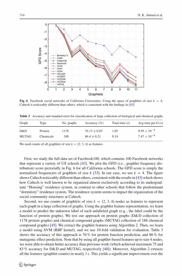
First, we study the full data set of Facebook100, which contains 100 Facebook networksthat represent a variety of US schools [43]. We plot the GFD (i.e. , graphlet frequency dis-tribution) score pictorially in Fig. 6 for all California schools. The GFD score is simply thenormalized frequencies of graphlets of size k [33]. In our case, we use k = 4. The figureshowsCaltech noticeably different than others, consistentwith the results in [43]which showshow Caltech is well known to be organized almost exclusively according to its undergrad-uate “Housing” residence system, in contrast to other schools that follow the predominant“dormitory” residence system. The residence system seems to impact the organization of thesocial community structures at Caltech.
Second, we use counts of graphlets of size k = {2, 3, 4}-nodes as features to representeach graph in a large collection of graphs. Using the graphlet feature representation, we learna model to predict the unknown label of each unlabeled graph (e.g. , the label could be thefunction of protein graphs). We test our approach on protein graphs (D&D collection of1178 protein graphs) and chemical compound graphs (MUTAG collection of 188 chemicalcompound graphs) [45]. We extract the graphlet features using Algorithm 2. Then, we learna model using SVM (RBF kernel), and we use 10-fold validation for evaluation. Table 3shows the accuracy of this approach is 76% for protein function prediction, and 86% formutagenic effect prediction. Note that by using all graphlet-based features up to size 4 nodes,we were able to obtain better accuracy than previous work (which achieved maximum 75 and83% accuracy for D&D and MUTAG, respectively [40]). Moreover, Algorithm 2 extractsall the features (graphlet counts) in nearly 1 s. This yields a significant improvement over the
123

Graphlet decomposition: framework, algorithms, and applications 715
graphlet feature extraction approach that was proposed in [40], which takes 2.45h to extractgraphlet features from the D&D collection.
Third, we compute graphlet counts on a 2 billion edge social network called Friendster.Friendster is an online gaming network. Before re-launching as a game Web site in 2011,Friendster was an online social network where users can form friendship links with eachothers. These data are provided by The Web Archive Project before the death of the socialnetwork. In these experiments, we use the induced subgraph of the nodes that either belong toat least one community or are connected to other nodes that belong to at least one community.Table 2 shows a significantly large number of 4-path (chains of 4 connected nodes) and 3-stars compared to the number of 4-cliques and triangles. Although the induced subgraph thatwe used from Friendster is clearly biased toward communities, the patterns that representcommunities, such as cliques and triangles, are less likely in the induced graph. For example,the frequency of 4-path patterns is 0.58, while the frequency of 4-cliques is 0.000014. Theseresults indicate that something wrong happened to the social network. Previous work onthe autopsy of Friendster showed that there was a collapse in the community structure ofFriendster, a cascade in user departure due to bad decisions in the design and interfacechanges. In a similar fashion, the low frequencyof community-related graphlets (e.g. , cliques)in Friendster also indicates the collapse of the social network.
6.2 Finding large stars, cliques, and other patterns fast
How can we quickly and efficiently find large cliques, stars, and other unique patterns?Further, how can we identify the top-k largest cliques, stars, etc.? Note that many of theseproblems are NP-hard, e.g. , finding the clique of maximum size is a well-known NP-hardproblem [17]. To answer these and other related queries, we leverage the proposed parallelgraphlet counting method in Algorithm 2.
Figure 7 provides a visualization of the human diseasome network [14], where we usedAlgorithm 2 to rank (weight) all the edges in the network by the number of star patterns ofsize 4 nodes. The intuition behind the method is that if an edge (or node) has a (relatively)large number of stars of 4 nodes (cliques, or another graphlet of interest), then it is also likelyto be part of a star of a large size. Recall that removing a node from a k-star or k-clique formsa star or clique of size k − 1 [17]. Accordingly, edges with large weights are likely to bemembers of large stars. Thus, as shown in Fig. 7, a visualization based on our fast graphletcounting method can help to quickly highlight such large stars by using the counts (of starsof size 4 nodes) as edge weights or colors.
Notably, Fig. 7 highlights the few phenotypes (such as colon cancer, leukemia, and deaf-ness) corresponding to hubs (large stars) that are connected to a large number of distinctdisorders, which is consistent with the findings in [14]. Note that the same approach is alsoapplicable for finding cliques and other interesting patterns, since edges with a high numberof 4-cliques are likely to be members of the largest clique in the network. Figure 8 showshow we can find large cliques in the terroristRel data [50].
6.3 Real-time visual graphlet mining
Visual analytics is the science of analytical reasoning facilitated by interactive visual inter-faces [6,42]. This work develops an interactive visual graph analytics platform based onthe proposed fast graphlet decomposition algorithm. In particular, we integrate interactive
123

716 N. K. Ahmed et al.
Fig. 7 Visualization of the human diseasome network: A network of disorders and disease genes linked byknown disorder–gene associations [14]. Edges are weighted/colored by their number of incident star graphletsof size 4 nodes; nodes are weighted/colored by their triangle counts. The large star on the right denoted by lightblue color corresponds to colon cancer; the large star on the lower left denoted by lime green color correspondsto deafness; and the large star on the right denoted by lime green color corresponds to leukemia. Notably, thisfigure highlights the few phenotypes (such as colon cancer, leukemia, and deafness) corresponding to hubs(large stars) that are connected to a large number of distinct disorders, which is consistent with [14] (colorfigure online)
visualization with our state-of-the-art parallel graphlet decomposition algorithm in orderto support discovery, analysis, and exploration of such data in real-time. We utilize thismulti-level graphlet analysis engine that uses graphlets as a basis for exploring, analyzing,and understanding complex networks interactively in real time. And, we highlight otherkey aspects including filtering, querying, ranking, manipulating, and a variety of multi-levelnetwork analysis and statistical techniques based on graphlets.
Notably, our proposed algorithm is shown to be fast and efficient for real-time interactiveexploration and mining of graphlets. We expect this tool to be extremely useful to biologistsand others interested in understanding biological (protein, brain networks, etc.) as well aschemical networks. There are a number of important and unique challenges in designing
123

Graphlet decomposition: framework, algorithms, and applications 717
Fig. 8 Visualization of the terroristRel network: A network of terrorists and their relationships. Terroristsare linked to each other if they contact each other, use the same facility, are members of the same family, orbelong to the same terrorist organization. Edges and nodes are weighted/colored by their number of incidentcliques of size 4 nodes. Notably, this figure highlights how the structure of terrorist networks is decomposed ofvarious clique patterns (terrorist organization) and how these cliques are interconnected. The figure highlightsthe largest clique on the top left denoted by dark blue (color figure online)
Fig. 9 Exploration of the brain neural network of C. Elegans [46] using our interactive graphlet visualanalytics tool. Nodes are colored by their k-core number and weighted by betweenness, whereas the links arecolored by eccentricity
123

718 N. K. Ahmed et al.
Fig. 10 Illustration of the graphlet methods for real-time interactive graphlet analysis. This demonstratesthe efficiency and effectiveness of the proposed methods for interactive real-time graphlet computations.In the screenshot above, the user selects a subgraph to interactively analyze via direct manipulation of thevisualization using the mouse. That is, the user adjusts the rectangular region above to highlight the subgraphsto analyze. The graphlet statistics are updated each time a node/edge is added or removed from the rectangularregion used to select the subgraph to explore via graphlets. Thus, the user can see how the graphlet statisticschange as nodes and edges are added (or removed) from the user-specified rectangular region (which in turnindicates the nodes and edges to include in the analysis). Note that we leverage localized graphlet updatemethods to achieve the performance required for real-time interactive graphlet mining and sense-making
methods for interactive exploration andmining of graphlets in real time. In particular, the real-time requirement of such a system is fast parallelmethods to achieve real-time interactive rates(e.g., with response times within microseconds or less). In particular, we derived dynamicupdate methods that are localized, that is, the update methods leverage the local structureof the graph for efficiently updating the counts when nodes/edges are selected, inserted,removed, etc. Thus, given a single node or edge, the method updates the graphlet counts forthat edge (as opposed to recomputing the full graphlet decomposition).
Figure 9 uses the interactive graphlet mining tool for real-time exploration of the brainneural network from C. Elegans [46]. Additionally, the tool is also useful for exploring manyother types of networks, e.g., a terrorist relationship network is shown in Fig. 10, whereasFig. 11 uses graphlets as a basis for understanding and characterizing the communities andtheir structure. As an aside, the graph in Fig. 11 is generated using the block Chung-Lu graphmodel. Thus, it is straightforward to see how graphlets can be used to characterize syntheticgraph generators and for evaluating their utility (e.g., if the synthetic graph preserves thedistribution of graphlets observed in a real-world network.).
The visual graphlet analytics tool is designed for rapid interactive visual exploration andgraph mining (Figs. 9, 10 and 11). Graphlets are computed on-the-fly upon a simple drag-and-drop of a graph file into the web browser. Additionally, the graphlet counts are updatedefficiently after each selection, insertion, deletion, or change to the graph data. Furthermore,
123

Graphlet decomposition: framework, algorithms, and applications 719
Fig. 11 Interactive graphlet exploration of community structure via direct manipulation and selection of thevisual representation
it is designed to be consistent with the way humans learn via immediate feedback upon everyuser interaction (e.g., change of a slider for filtering) [1,42]. Users have rapid, incremental,and reversible control over all graph queries with immediate and continuous visual feedback.
7 Conclusion and future work
In this paper, we proposed a fast, efficient, and parallel framework as well as a family ofalgorithms for counting k-node graphlets. We provided a novel theoretical analysis of com-binatorial arguments that capture the relationships between various graphlets. The proposedframework leverages these combinatorial arguments to obtain significant improvement onthe scalability of graphlet counting. For each edge, we count a few graphlets and obtain theexact counts of others in constant time using the combinatorial arguments. We systematicallyinvestigate the scalability of our algorithm on a large collection of 300+ networks from avariety of domains. Finally, we provided a systematic investigation across a variety of existingand new applications for graphlet counting, such as finding unique patterns in graphs, graphsimilarity, and graph classification. In future work, we aim to extend our proposed frameworkto higher-order graphlets, as well as extend our approach to the distributed setting.
References
1. Ahlberg C,Williamson C, Shneiderman B (1992) Dynamic queries for information exploration: an imple-mentation and evaluation. In: Proceedings of SIGCHI, pp 619–626
2. Ahmed NK, Duffield N, Neville J, Kompella R (2014) Graph sample and hold: a framework for big-graphanalytics. In: SIGKDD
3. Ahmed NK, Neville J, Kompella R (2010) Reconsidering the foundations of network sampling. In:Proceedings of the 2nd Workshop on Information in Networks
4. Ahmed NK, Neville J, Kompella R (2012) Space-efficient sampling from social activity streams. In:Proceedings of the 1st international workshop on big data, streams and heterogeneous source mining:algorithms, systems, programming models and applications, pp 53–60
123

720 N. K. Ahmed et al.
5. Ahmed NK, Neville J, Kompella R (2014) Network sampling: from static to streaming graphs. ACMTrans Knowl Discov Data (TKDD) 8(2):1–56
6. Ahmed NK, Rossi RA (2015) Interactive visual graph analytics on the web. In: Proceedings of the NinthInternational AAAI Conference on Web and Social Media
7. Becchetti L, Boldi P, Castillo C, Gionis A (2008) Efficient semi-streaming algorithms for local trianglecounting in massive graphs. In: SIGKDD
8. BhuiyanMA, RahmanM, RahmanM, Al HasanM (2012) Guise: uniform sampling of graphlets for largegraph analysis. In: ICDM
9. Costa F, De Grave K (2010) Fast neighborhood subgraph pairwise distance kernel. In: ICML10. Faust K (2010) A puzzle concerning triads in social networks: graph constraints and the triad census. Soc
Netw 32(3):221–23311. Feldman D, Shavitt Y (2008) Automatic large scale generation of internet pop level maps. In: IEEE
GLOBECOM12. Frank O (1988) Triad count statistics. Ann Discrete Math 38:141–14913. Getoor L, Taskar B (2007) Introduction to statistical relational learning. MIT Press, Cambridge14. Goh K-I, Cusick ME, Valle D, Childs B, Vidal M, Barabási A-L (2007) The human disease network.
PNAS 104(21):8685–869015. Gonen M, Shavitt Y (2009) Approximating the number of network motifs. Internet Math 6(3):349–37216. Granovetter M (1983) The strength of weak ties: a network theory revisited. Sociol Theory 1(1):201–23317. Gross JL, Yellen J, Zhang P (2013) Handbook of graph theory, 2nd edn. Chapman & Hall, London18. Hales D, Arteconi S (2008) Motifs in evolving cooperative networks look like protein structure networks.
J Netw Heterog Media 3(2):239–24919. HayesW,SunK, PržuljN (2013)Graphlet-basedmeasures are suitable for biological network comparison.
Bioinformatics 29(4):483–49120. Hocevar T, Demšar J (2014) A combinatorial approach to graphlet counting. Bioinformatics 30(4):559–
56521. Holland PW, Leinhardt S (1976) Local structure in social networks. Sociol Methodol 7:1–4522. Kashima H, Saigo H, Hattori M, Tsuda K (2010) Graph kernels for chemoinformatics. Chemoinfor-
matics and advanced machine learning perspectives: complex computational methods and collaborativetechniques, p 1
23. Kelly PJ (1957) A congruence theorem for trees. Pac J Math 7(1):961–96824. Kloks T, Kratsch D, Müller H (2000) Finding and counting small induced subgraphs efficiently. Inf
Process Lett 74(3):115–12125. Kuchaiev O, Milenkovic T, Memiševic V, Hayes W, Pržulj N (2010) Topological network alignment
uncovers biological function and phylogeny. J R Soc Interface 7(50):1341–135426. Manvel B, Stockmeyer PK (1971) On reconstruction of matrices. Math Mag 44:218–22127. Marcus D, Shavitt Y (2012) Rage—a rapid graphlet enumerator for large networks. Comput Netw
56(2):810–81928. McKay BD (1997) Small graphs are reconstructible. Australas J Comb 15:123–12629. Milenkoviæ T, Pržulj N (2008) Uncovering biological network function via graphlet degree signatures.
Cancer Inform 6:25730. Milenkovic T,NgWL,HayesW, Pržulj N (2010)Optimal network alignmentwith graphlet degree vectors.
Cancer Inform 9:12131. MiloR, Shen-Orr S, Itzkovitz S,KashtanN,ChklovskiiD,AlonU (2002)Networkmotifs: simple building
blocks of complex networks. Science 298(5594):824–82732. Noble CC, Cook DJ (2003) Graph-based anomaly detection. In: SIGKDD33. Pržulj N, Corneil DG, Jurisica I (2004) Modeling interactome: scale-free or geometric? Bioinformatics
20(18):3508–351534. Ralaivola L, Swamidass SJ, Saigo H, Baldi P (2005) Graph kernels for chemical informatics. Neural
Netw 18(8):1093–111035. Rossi RA, Ahmed NK (2015a) The network data repository with interactive graph analytics and visual-
ization. In: Proceedings of the twenty-ninth AAAI conference on artificial intelligence36. Rossi RA, Gallagher B, Neville J, Henderson K (2013) Modeling dynamic behavior in large evolving
graphs. In: Proceedings of WSDM, pp 667–67637. Rossi RA, McDowell LK, Aha DW, Neville J (2012) Transforming graph data for statistical relational
learning. J Artif Intell Res 45(1):363–44138. Rossi R, Ahmed N (2015b) Role discovery in networks. In: TKDE39. Schaeffer SE (2007) Graph clustering. Comput Sci Rev 1(1):27–6440. Shervashidze N, Petri T, Mehlhorn K, Borgwardt KM, Vishwanathan S (2009) Efficient graphlet kernels
for large graph comparison. In: AISTATS
123

Graphlet decomposition: framework, algorithms, and applications 721
41. Stanley RP (1986) What is enumerative combinatorics?. Springer, Berlin42. Thomas JJ, Cook KA (2005) Illuminating the path: the research and development agenda for visual
analytics. IEEE Computer Society, Washington43. Traud AL,Mucha PJ, Porter MA (2012) Social structure of facebook networks. Physica A 391(16):4165–
418044. Ugander J, Backstrom L, Kleinberg J (2013) Subgraph frequencies: mapping the empirical and extremal
geography of large graph collections. In: WWW45. Vishwanathan SVN, Schraudolph NN, Kondor R, Borgwardt KM (2010) Graph kernels. JMLR 11:1201–
124246. Watts D, Strogatz S (1998) Collective dynamics of small-world networks. Nature 393(6684):440–44247. Wernicke S, Rasche F (2006) Fanmod: a tool for fast networkmotif detection. Bioinformatics 22(9):1152–
115348. Zhang L, Han Y, Yang Y, Song M, Yan S, Tian Q (2013) Discovering discriminative graphlets for aerial
image categories recognition. IEEE Trans Image Process 22(12):5071–508449. Zhang L, SongM, Liu Z, LiuX, Bu J, ChenC (2013) Probabilistic graphlet cut: exploiting spatial structure
cue for weakly supervised image segmentation. In: CVPR50. Zhao B, Sen P, Getoor L (2006) Event classification and relationship labeling in affiliation networks. In:
ICML Workshop on Statistical Network Analysis (SNA)
Nesreen K. Ahmed is a Research Scientist at Intel Labs. She receivedher Ph.D. from the Computer Science Department at Purdue Universityin 2015, and her M.S. in statistics and computer science from PurdueUniversity in 2014. She was a visiting researcher at Facebook data sci-ence, Adobe Labs, Technicolor Labs, and Intel analytics. Her researchinterests include machine learning, data mining, the theory and algo-rithms of large-scale graph mining, relational machine learning, andtheir applications in social and information networks. Dr. Ahmed hasauthored numerous papers/tutorials in top-tier conferences/journals.Her research was selected among the best papers of ICDM in 2015and BigMine in 2012 and covered by popular press such as the MITTechnology Review. She was selected by UC Berkeley among the topfemale rising stars in computer science and engineering in 2014. Dr.Ahmed holds 2 U.S. patents filed by Adobe and co-authored the opensource network data repository (http://networkrepository.com).
Jennifer Neville is the Miller Family Chair Associate Professor ofComputer Science and Statistics at Purdue University. She received herPh.D. from the University of Massachusetts Amherst in 2006. In 2016,she was the PC chair of the 9th ACM International Conference on WebSearch and Data. In 2012, she was awarded an NSF Career Award;in 2008, she was chosen by IEEE as one of “AI’s 10 to watch”; andin 2007, she was selected as a member of the DARPA Computer Sci-ence Study Group. Her research focuses on developing data miningand machine learning techniques for relational domains, which includesocial, information, and physical networks.
123

722 N. K. Ahmed et al.
Ryan A. Rossi is a research scientist at Palo Alto Research Center(PARC). His research is grounded in machine learning and spans the-ory, algorithms, and applications of large relational (graph/network)data that arise from social and physical phenomena. Before joiningPARC, Dr. Rossi worked at various industrial, government, and aca-demic research laboratories including Lawrence Livermore NationalLaboratory (LLNL), Naval Research Laboratory (NRL), NASA JetPropulsion Laboratory (JPL), University of Massachusetts Amherst,among others. Dr. Rossi earned his Ph.D. and M.S. in Computer Sci-ence at Purdue University. His dissertation work focused on relationalmachine learning and mining of dynamic networks. Dr. Rossi is a recip-ient of the NSF Graduate Research Fellowship (NSF GRFP), NationalDefense Science and Engineering Graduate Fellowship (NDSEG), aswell as two Purdue University Fellowships. He has authored numer-ous papers at top conferences and journals as well as a number ofpatents. He also co-founded the network repository project (http://networkrepository.com).
Nick G. Duffield is a Professor in Electrical and Computer Engineer-ing at Texas A&M University, and Director of the Texas A&M Engi-neering Big Data Initiative. From 1995 until 2013, he worked at AT&TLabs Research, Florham Park, NJ, where he was a Distinguished Mem-ber of Technical Staff and an AT&T Fellow. He also held positionsin Dublin, Ireland, Heidelberg, Germany, and Rutgers University, NJ.He received a BA (1982) and a MMath (1983) from the University ofCambridge, UK, and a Ph.D. (1987) in Mathematical Physics from theUniversity of London, UK. His research focuses on data science and itapplications. He is Chief Editor for Big Data at Frontiers in ICT, anEditor-at-Large for the IEEE/ACM Transactions on Networking, anda member of the board of directors of ACM SIGMETRICS. He is anIEEE and IET Fellow and was a co-recipient of the ACM SIGMET-RICS Test of Time Award in 2012 and 2013.
Theodore L. Willke received the EngScD degree with distinction fromColumbia University in 2010. His research interests include parallelcomputing, image processing, machine learning, graph analytics, andcognitive neuroscience. He is the recipient of the IEEE/MILCOM post-graduate fellowship and two US Department of Energy graduate fel-lowships. He has authored over 25 papers and holds 14 patents. He wonthe MASCOTS Best Paper Award in 2013 for work on MapReduce per-formance modeling. He is currently a Senior Principal Engineer withIntel Labs, where his team focuses on parallel computing challenges.He is also a co-principal investigator in a multi-year grand challengeproject on real-time brain decoding with the Princeton NeuroscienceInstitute. Previously, he founded an Intel venture focused on graph ana-lytics for data science that is now an open source project. In 2014, hewon Intel’s highest award for this effort. In 2015, he was appointed tothe Science and Technology Advisory Committee of the US Depart-ment of Homeland Security.
123