Graphics Programming

Principles and Algorithms

Zongli Shi

May 27, 2017

Abstract

This paper is an introduction to graphics programming. This is a computer science fieldtrying to answer questions such as how we can model 2D and 3D objects and have them displayedon screen. Researchers in this field are constantly trying to find more efficient algorithms forthese tasks. We are going to look at basic algorithms for modeling and drawing line segments,2D and 3D polygons. We are also going to explore ways to transform and clip 2D and 3Dpolygons. For illustration purpose, the algorithms presented in this paper are implemented inC++ and hosted at GitHub. Link to the GitHub repository can be found in the introductionparagraph.

1 Introduction

Computer graphics has been playing a vital role in communicating computer-generated informationto human users as well as providing a more intuitive way for users to interact with computers. Al-though nowadays, devices such as touch screens are everywhere, the effort of developing graphicssystem in the first place and beauty of efficient graphics rendering algorithms should not be underes-timated. Future development in graphics hardware will also bring new challenges, which will requireus to have a thorough understanding of the fundamentals. This paper will mostly investigate thevarious problems in graphics programming and the algorithms to solve them. All of the algorithmsare also presented in the book Computer Graphics by Steven Harrington [Har87]. This paper willalso serve as a tutorial, instructing the readers to build a complete graphics system from scratch. Atthe end we shall have a program manipulating basic bits and bytes but capable of generating 3-Danimation all by itself. To better assist the reader in implementing the algorithms presented in thispaper, the writer’s implementation in C++ can be found in the following GitHub link:

https://github.com/shizongli94/graphics_programming.

2 Basic Problems in Graphics

The basic problems in graphics programming are similar to those in any task of approximation. Thenotion of shapes such as polygons and lines are abstract, and by their definitions, continuous intheir nature. A line can extend to both directions forever. A polygon can be made as large as wewant. However, most display devices are represented as a rectangle holding finitely many individualdisplaying units called pixels. The size of the screen limits the size of our shapes and the amountof pixels limit how much detail we can put on screen. Therefore, we are trying to map somethingcontinuous and infinite in nature such as lines and polygons to something discrete and finite. In thisprocess, some information has to be lost but we should also try to approximate the best we can.We will first look at how to draw a line on screen to illustrate the process of building a discreterepresentation and how to recover as much lost information as we can.

1

3 Drawing a Line Segment

Since a line is infinite in its nature, we have to restrict ourselves to drawing line segments, which willa be reasonable representation of infinite line when going from one side of a screen to another. Thesimplest way to represent a line segment is to have the coordinates of its two end points. One wayof drawing a line segment will be simply starting with one end point and on the way of approachingthe other, turning on pixels.

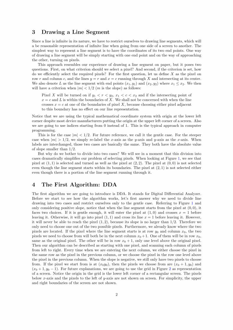
This approach resembles our experience of drawing a line segment on paper, but it poses twoquestions. First, on what criterion should we select a pixel? And second, if the criterion is set, howdo we efficiently select the required pixels? For the first question, let us define X as the pixel onrow r and column c, and the lines y = r and x = c running through X and intersecting at its center.We also denote L as the line segment with end points (x1, y1) and (x2, y2) where x1 ≤ x2. We thenwill have a criterion when |m| < 1/2 (m is the slope) as follows:

Pixel X will be turned on if y1 < r < y2, x1 < c < x2 and if the intersecting point ofx = c and L is within the boundaries of X. We shall not be concerned with when the linecrosses x = c at one of the boundaries of pixel X, because choosing either pixel adjacentto this boundary has no effect on our line representation.

Notice that we are using the typical mathematical coordinate system with origin at the lower leftcorner despite most device manufacturers putting the origin at the upper left corner of a screen. Alsowe are going to use indices starting from 0 instead of 1. This is the typical approach in computerprogramming.

This is for the case |m| < 1/2. For future reference, we call it the gentle case. For the steepercase when |m| > 1/2, we simply re-label the x-axis as the y-axis and y-axis as the x-axis. Whenlabels are interchanged, those two cases are basically the same. They both have the absolute valueof slope smaller than 1/2.

But why do we bother to divide into two cases? We will see in a moment that this division intocases dramatically simplifies our problem of selecting pixels. When looking at Figure 1, we see thatpixel at (1, 1) is selected and turned as well as the pixel at (2, 2). The pixel at (0, 0) is not selectedeven though the line segment starts within its boundaries. The pixel at (2, 1) is not selected eithereven though there is a portion of the line segment running through it.

4 The First Algorithm: DDA

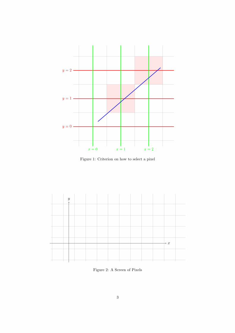
The first algorithm we are going to introduce is DDA. It stands for Digital Differential Analyzer.Before we start to see how the algorithm works, let’s first answer why we need to divide linedrawing into two cases and restrict ourselves only to the gentle case. Referring to Figure 1 andonly considering positive slope, notice that when the line segment starts from the pixel at (0, 0), itfaces two choices. If it is gentle enough, it will enter the pixel at (1, 0) and crosses x = 1 beforeleaving it. Otherwise, it will go into pixel (1, 1) and cross its line x = 1 before leaving it. However,it will never be able to reach the pixel (1, 2), because its slope is no larger than 1/2. Therefore weonly need to choose one out of the two possible pixels. Furthermore, we already know where the twopixels are located. If the pixel where the line segment starts is at row y0 and column x0, the twopixels we need to choose from will both be in the next column x0 +1. One of them will be in row x0,same as the original pixel. The other will be in row x0 + 1, only one level above the original pixel.Then our algorithm can be described as starting with one pixel, and scanning each column of pixelsfrom left to right. Every time when we are entering the next column, we either choose the pixel inthe same row as the pixel in the previous column, or we choose the pixel in the row one level abovethe pixel in the previous column. When the slope is negative, we still only have two pixels to choosefrom. If the pixel we start from is at (x0y0), then the pixels we choose from are (x0 + 1, y0) and(x0 + 1, y0 − 1). For future explanations, we are going to use the grid in Figure 2 as representationof a screen. Notice the origin in the grid is the lower left corner of a rectangular screen. The pixelsbelow x-axis and the pixels to the left of y-axis are not shown on screen. For simplicity, the upperand right boundaries of the screen are not shown.

2

y = 0

y = 1

y = 2

x = 0 x = 1 x = 2

Figure 1: Criterion on how to select a pixel

x

y

Figure 2: A Screen of Pixels

3

B0

P0

x

y

Figure 3: An Example of DDA Algorithm

B1

P1

x

y

Figure 4: The state of the program right after coloring a pixel in the second column

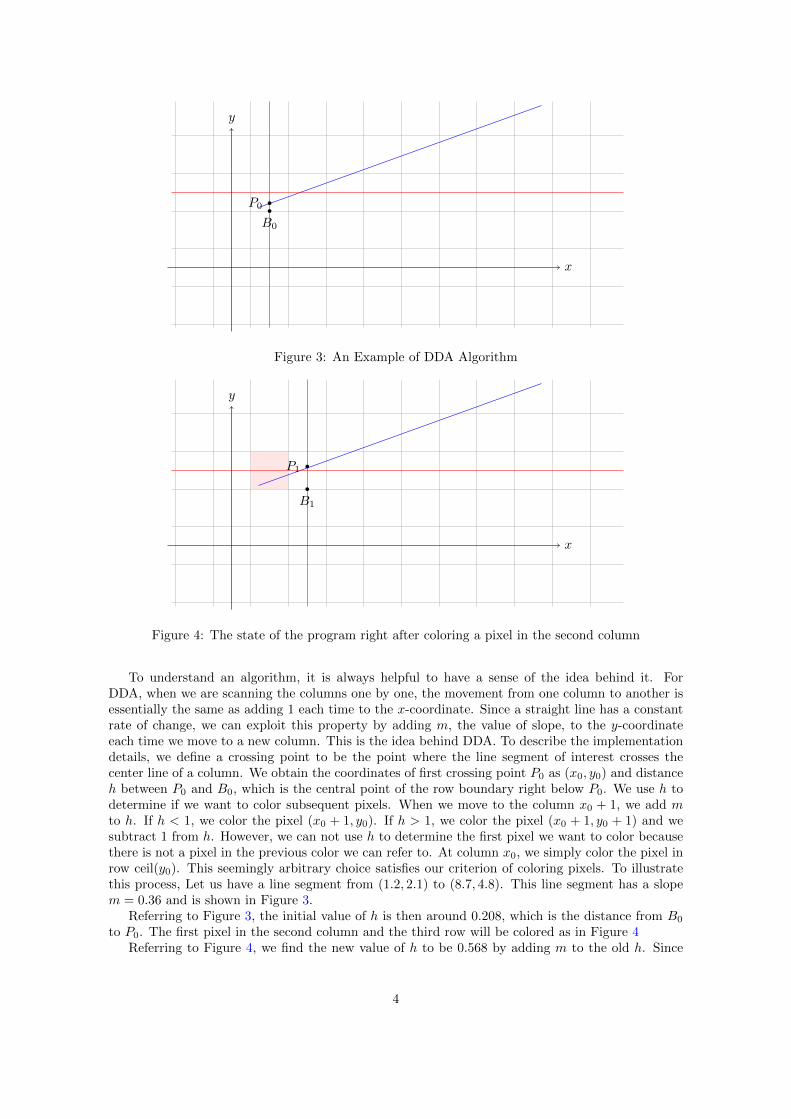
To understand an algorithm, it is always helpful to have a sense of the idea behind it. ForDDA, when we are scanning the columns one by one, the movement from one column to another isessentially the same as adding 1 each time to the x-coordinate. Since a straight line has a constantrate of change, we can exploit this property by adding m, the value of slope, to the y-coordinateeach time we move to a new column. This is the idea behind DDA. To describe the implementationdetails, we define a crossing point to be the point where the line segment of interest crosses thecenter line of a column. We obtain the coordinates of first crossing point P0 as (x0, y0) and distanceh between P0 and B0, which is the central point of the row boundary right below P0. We use h todetermine if we want to color subsequent pixels. When we move to the column x0 + 1, we add mto h. If h < 1, we color the pixel (x0 + 1, y0). If h > 1, we color the pixel (x0 + 1, y0 + 1) and wesubtract 1 from h. However, we can not use h to determine the first pixel we want to color becausethere is not a pixel in the previous color we can refer to. At column x0, we simply color the pixel inrow ceil(y0). This seemingly arbitrary choice satisfies our criterion of coloring pixels. To illustratethis process, Let us have a line segment from (1.2, 2.1) to (8.7, 4.8). This line segment has a slopem = 0.36 and is shown in Figure 3.

Referring to Figure 3, the initial value of h is then around 0.208, which is the distance from B0

to P0. The first pixel in the second column and the third row will be colored as in Figure 4Referring to Figure 4, we find the new value of h to be 0.568 by adding m to the old h. Since

4

B′3

P3

x

y

Figure 5: The state of the program right after coloring a pixel in the fourth column

x

y

Figure 6: The state of the program right after coloring a pixel in the fifth column

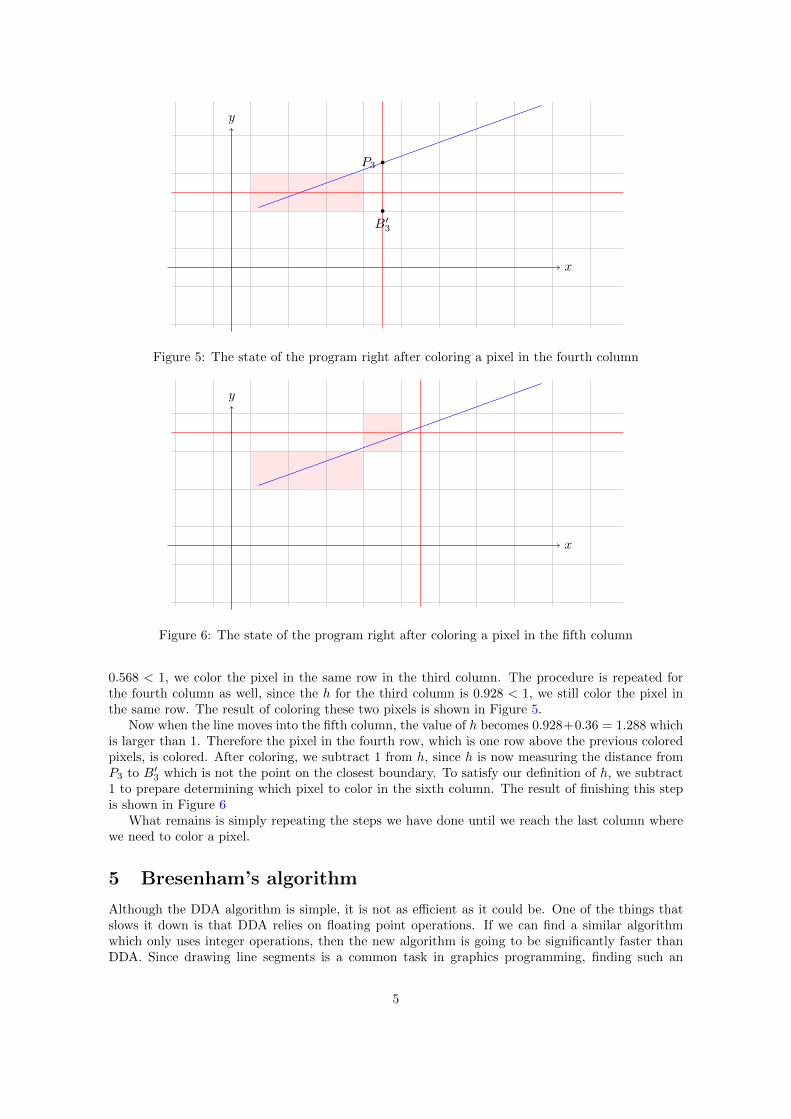
0.568 < 1, we color the pixel in the same row in the third column. The procedure is repeated forthe fourth column as well, since the h for the third column is 0.928 < 1, we still color the pixel inthe same row. The result of coloring these two pixels is shown in Figure 5.

Now when the line moves into the fifth column, the value of h becomes 0.928+0.36 = 1.288 whichis larger than 1. Therefore the pixel in the fourth row, which is one row above the previous coloredpixels, is colored. After coloring, we subtract 1 from h, since h is now measuring the distance fromP3 to B′3 which is not the point on the closest boundary. To satisfy our definition of h, we subtract1 to prepare determining which pixel to color in the sixth column. The result of finishing this stepis shown in Figure 6

What remains is simply repeating the steps we have done until we reach the last column wherewe need to color a pixel.

5 Bresenham’s algorithm

Although the DDA algorithm is simple, it is not as efficient as it could be. One of the things thatslows it down is that DDA relies on floating point operations. If we can find a similar algorithmwhich only uses integer operations, then the new algorithm is going to be significantly faster thanDDA. Since drawing line segments is a common task in graphics programming, finding such an

5

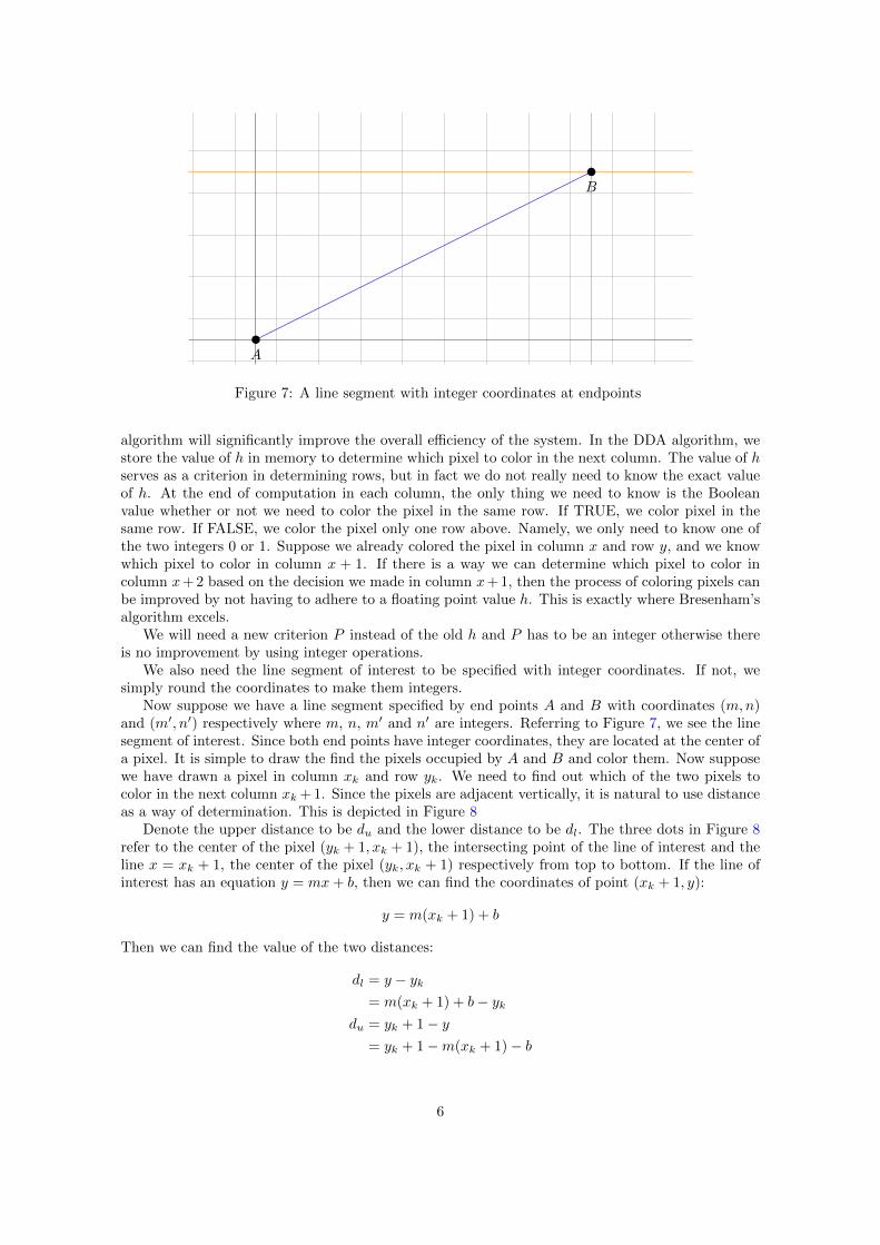
A

B

Figure 7: A line segment with integer coordinates at endpoints

algorithm will significantly improve the overall efficiency of the system. In the DDA algorithm, westore the value of h in memory to determine which pixel to color in the next column. The value of hserves as a criterion in determining rows, but in fact we do not really need to know the exact valueof h. At the end of computation in each column, the only thing we need to know is the Booleanvalue whether or not we need to color the pixel in the same row. If TRUE, we color pixel in thesame row. If FALSE, we color the pixel only one row above. Namely, we only need to know one ofthe two integers 0 or 1. Suppose we already colored the pixel in column x and row y, and we knowwhich pixel to color in column x + 1. If there is a way we can determine which pixel to color incolumn x+ 2 based on the decision we made in column x+ 1, then the process of coloring pixels canbe improved by not having to adhere to a floating point value h. This is exactly where Bresenham’salgorithm excels.

We will need a new criterion P instead of the old h and P has to be an integer otherwise thereis no improvement by using integer operations.

We also need the line segment of interest to be specified with integer coordinates. If not, wesimply round the coordinates to make them integers.

Now suppose we have a line segment specified by end points A and B with coordinates (m,n)and (m′, n′) respectively where m, n, m′ and n′ are integers. Referring to Figure 7, we see the linesegment of interest. Since both end points have integer coordinates, they are located at the center ofa pixel. It is simple to draw the find the pixels occupied by A and B and color them. Now supposewe have drawn a pixel in column xk and row yk. We need to find out which of the two pixels tocolor in the next column xk + 1. Since the pixels are adjacent vertically, it is natural to use distanceas a way of determination. This is depicted in Figure 8

Denote the upper distance to be du and the lower distance to be dl. The three dots in Figure 8refer to the center of the pixel (yk + 1, xk + 1), the intersecting point of the line of interest and theline x = xk + 1, the center of the pixel (yk, xk + 1) respectively from top to bottom. If the line ofinterest has an equation y = mx+ b, then we can find the coordinates of point (xk + 1, y):

y = m(xk + 1) + b

Then we can find the value of the two distances:

dl = y − yk= m(xk + 1) + b− yk

du = yk + 1− y= yk + 1−m(xk + 1)− b

6

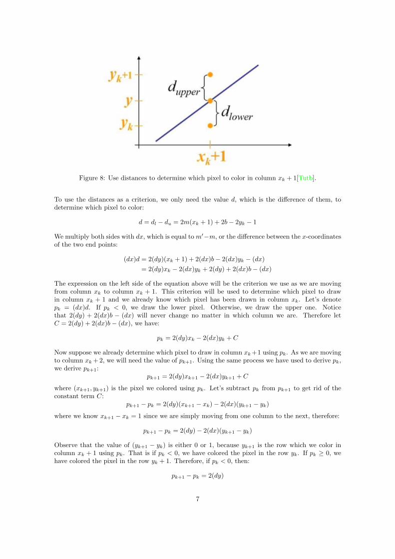
Figure 8: Use distances to determine which pixel to color in column xk + 1[Tutb].

To use the distances as a criterion, we only need the value d, which is the difference of them, todetermine which pixel to color:

d = dl − du = 2m(xk + 1) + 2b− 2yk − 1

We multiply both sides with dx, which is equal to m′−m, or the difference between the x-coordinatesof the two end points:

(dx)d = 2(dy)(xk + 1) + 2(dx)b− 2(dx)yk − (dx)

= 2(dy)xk − 2(dx)yk + 2(dy) + 2(dx)b− (dx)

The expression on the left side of the equation above will be the criterion we use as we are movingfrom column xk to column xk + 1. This criterion will be used to determine which pixel to drawin column xk + 1 and we already know which pixel has been drawn in column xk. Let’s denotepk = (dx)d. If pk < 0, we draw the lower pixel. Otherwise, we draw the upper one. Noticethat 2(dy) + 2(dx)b − (dx) will never change no matter in which column we are. Therefore letC = 2(dy) + 2(dx)b− (dx), we have:

pk = 2(dy)xk − 2(dx)yk + C

Now suppose we already determine which pixel to draw in column xk +1 using pk. As we are movingto column xk + 2, we will need the value of pk+1. Using the same process we have used to derive pk,we derive pk+1:

pk+1 = 2(dy)xk+1 − 2(dx)yk+1 + C

where (xk+1, yk+1) is the pixel we colored using pk. Let’s subtract pk from pk+1 to get rid of theconstant term C:

pk+1 − pk = 2(dy)(xk+1 − xk)− 2(dx)(yk+1 − yk)

where we know xk+1 − xk = 1 since we are simply moving from one column to the next, therefore:

pk+1 − pk = 2(dy)− 2(dx)(yk+1 − yk)

Observe that the value of (yk+1 − yk) is either 0 or 1, because yk+1 is the row which we color incolumn xk + 1 using pk. That is if pk < 0, we have colored the pixel in the row yk. If pk ≥ 0, wehave colored the pixel in the row yk + 1. Therefore, if pk < 0, then:

pk+1 − pk = 2(dy)

7

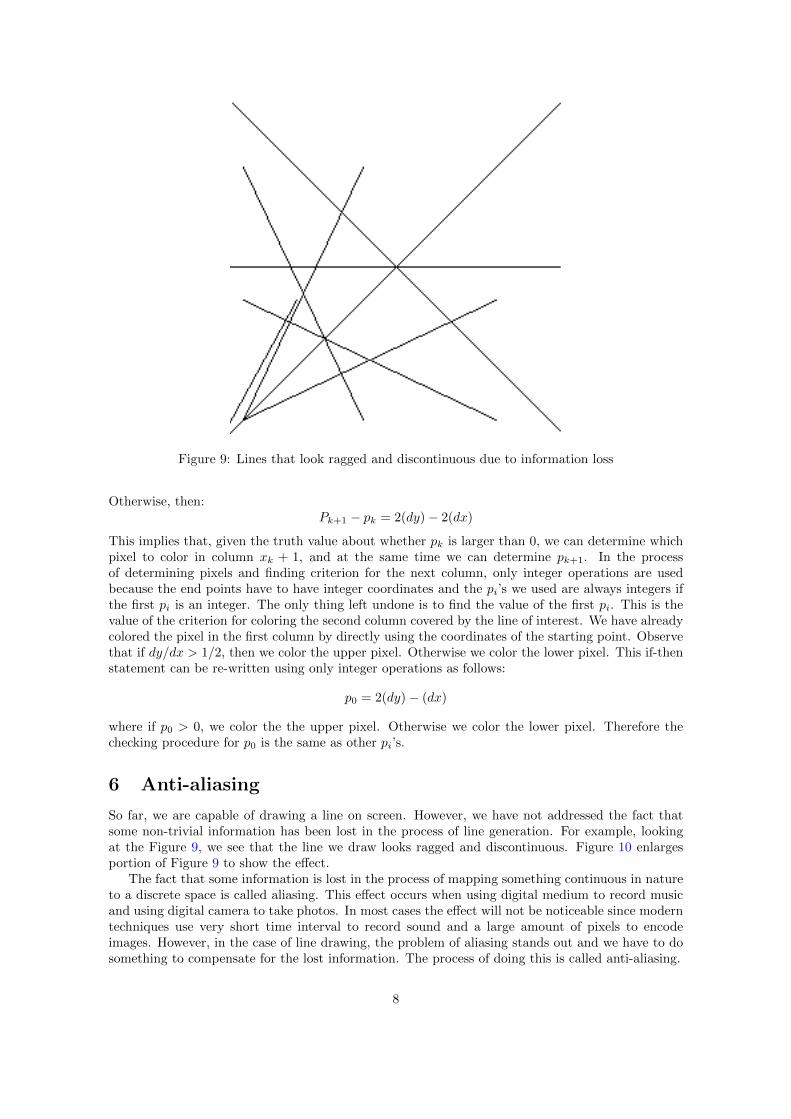
Figure 9: Lines that look ragged and discontinuous due to information loss

Otherwise, then:Pk+1 − pk = 2(dy)− 2(dx)

This implies that, given the truth value about whether pk is larger than 0, we can determine whichpixel to color in column xk + 1, and at the same time we can determine pk+1. In the processof determining pixels and finding criterion for the next column, only integer operations are usedbecause the end points have to have integer coordinates and the pi’s we used are always integers ifthe first pi is an integer. The only thing left undone is to find the value of the first pi. This is thevalue of the criterion for coloring the second column covered by the line of interest. We have alreadycolored the pixel in the first column by directly using the coordinates of the starting point. Observethat if dy/dx > 1/2, then we color the upper pixel. Otherwise we color the lower pixel. This if-thenstatement can be re-written using only integer operations as follows:

p0 = 2(dy)− (dx)

where if p0 > 0, we color the the upper pixel. Otherwise we color the lower pixel. Therefore thechecking procedure for p0 is the same as other pi’s.

6 Anti-aliasing

So far, we are capable of drawing a line on screen. However, we have not addressed the fact thatsome non-trivial information has been lost in the process of line generation. For example, lookingat the Figure 9, we see that the line we draw looks ragged and discontinuous. Figure 10 enlargesportion of Figure 9 to show the effect.

The fact that some information is lost in the process of mapping something continuous in natureto a discrete space is called aliasing. This effect occurs when using digital medium to record musicand using digital camera to take photos. In most cases the effect will not be noticeable since moderntechniques use very short time interval to record sound and a large amount of pixels to encodeimages. However, in the case of line drawing, the problem of aliasing stands out and we have to dosomething to compensate for the lost information. The process of doing this is called anti-aliasing.

8

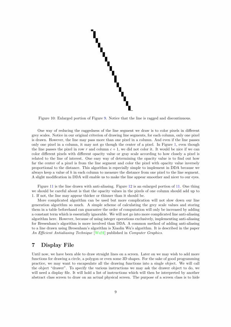
Figure 10: Enlarged portion of Figure 9. Notice that the line is ragged and discontinuous.

One way of reducing the raggedness of the line segment we draw is to color pixels in differentgrey scales. Notice in our original criterion of drawing line segments, for each column, only one pixelis drawn. However, the line may pass more than one pixel in a column. And even if the line passesonly one pixel in a column, it may not go though the center of a pixel. In Figure 1, even thoughthe line passes the pixel in row r and column c+ 1, we did not color it. It would be nice if we cancolor different pixels with different opacity value or gray scale according to how closely a pixel isrelated to the line of interest. One easy way of determining the opacity value is to find out howfar the center of a pixel is from the line segment and color the pixel with opacity value inverselyproportional to the distance. This algorithm is especially simple to implement in DDA because wealways keep a value of h in each column to measure the distance from one pixel to the line segment.A slight modification in DDA will enable us to make the line appear smoother and nicer to our eyes.

Figure 11 is the line drawn with anti-aliasing. Figure 12 is an enlarged portion of 11. One thingwe should be careful about is that the opacity values in the pixels of one column should add up to1. If not, the line may appear thicker or thinner than it should be.

More complicated algorithm can be used but more complication will not slow down our linegeneration algorithm so much. A simple scheme of calculating the grey scale values and storingthem in a table beforehand can guarantee the order of computation will only be increased by addinga constant term which is essentially ignorable. We will not go into more complicated line anti-aliasingalgorithm here. However, because of using integer operations exclusively, implementing anti-aliasingfor Bresenham’s algorithm is more involved than DDA. A common method of adding anti-aliasingto a line drawn using Bresenham’s algorithm is Xiaolin Wu’s algorithm. It is described in the paperAn Efficient Antialiasing Technique [Wu91] published in Computer Graphics.

7 Display File

Until now, we have been able to draw straight lines on a screen. Later on we may wish to add morefunctions for drawing a circle, a polygon or even some 3D shapes. For the sake of good programmingpractice, we may want to encapsulate all the drawing functions into a single object. We will callthe object “drawer”. To specify the various instructions we may ask the drawer object to do, wewill need a display file. It will hold a list of instructions which will then be interpreted by anotherabstract class screen to draw on an actual physical screen. The purpose of a screen class is to hide

9

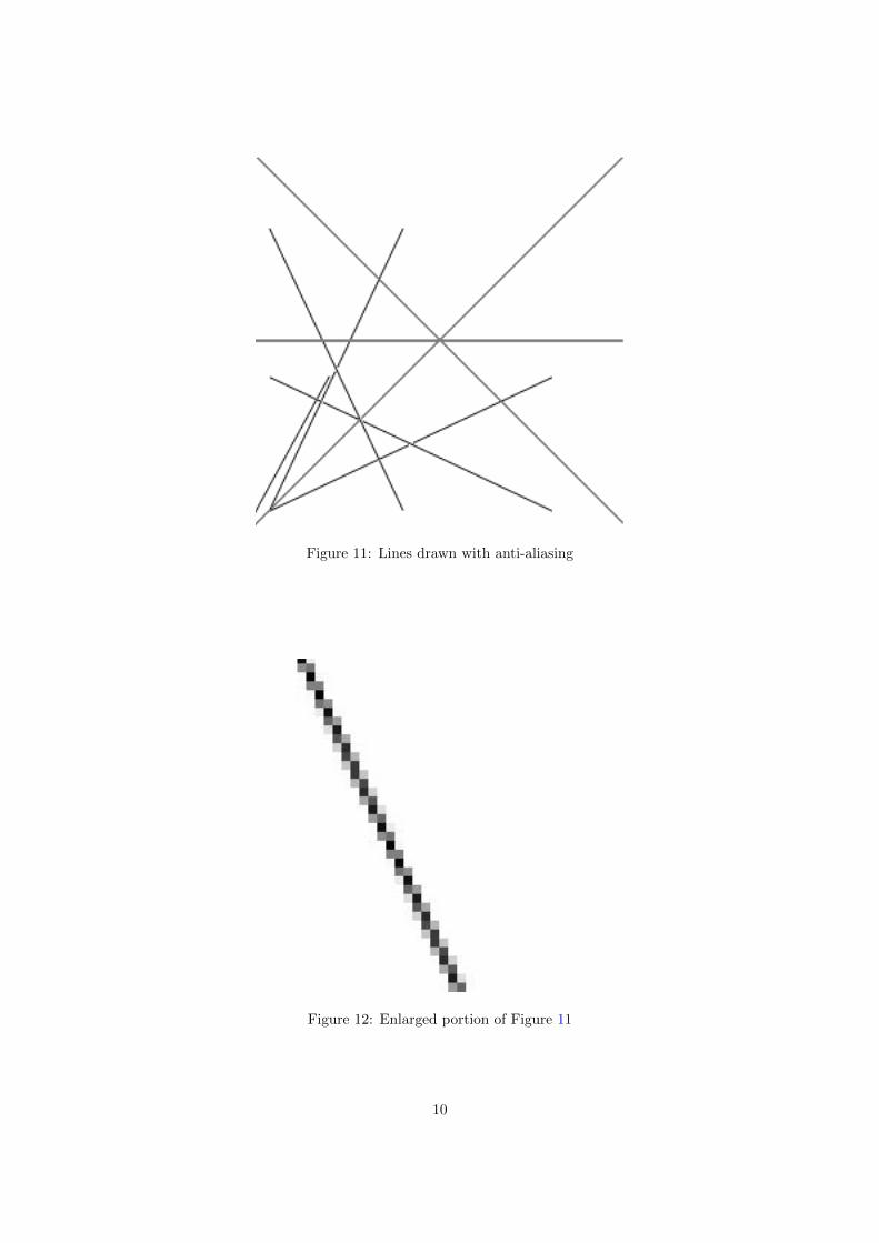
Figure 11: Lines drawn with anti-aliasing

Figure 12: Enlarged portion of Figure 11

10

away the messy details for a specific type of screen. It also offers a common interface for differenttypes of screens, so our drawing commands in display file will be transportable across different kindsof hardware. The only assumption made about the three classes is that we restrict ourselves to drawon a rectangular screen and the pixels are represented as a grid.

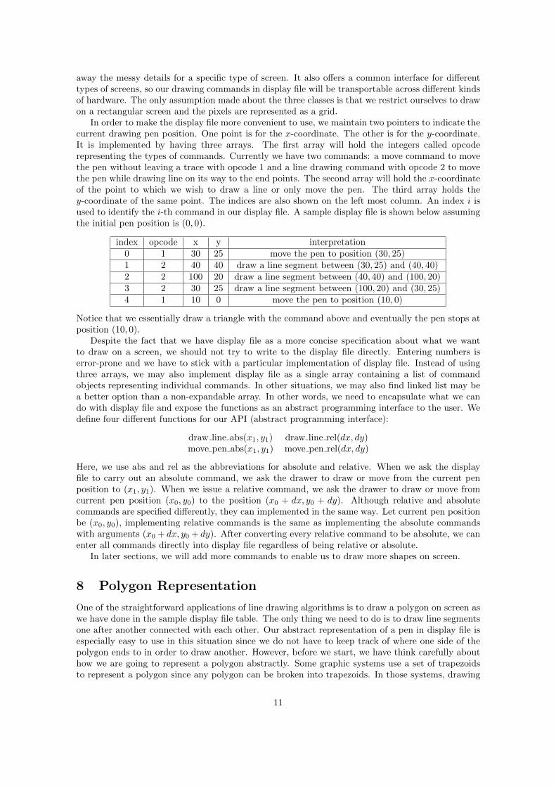
In order to make the display file more convenient to use, we maintain two pointers to indicate thecurrent drawing pen position. One point is for the x-coordinate. The other is for the y-coordinate.It is implemented by having three arrays. The first array will hold the integers called opcoderepresenting the types of commands. Currently we have two commands: a move command to movethe pen without leaving a trace with opcode 1 and a line drawing command with opcode 2 to movethe pen while drawing line on its way to the end points. The second array will hold the x-coordinateof the point to which we wish to draw a line or only move the pen. The third array holds they-coordinate of the same point. The indices are also shown on the left most column. An index i isused to identify the i-th command in our display file. A sample display file is shown below assumingthe initial pen position is (0, 0).

index opcode x y interpretation0 1 30 25 move the pen to position (30, 25)1 2 40 40 draw a line segment between (30, 25) and (40, 40)2 2 100 20 draw a line segment between (40, 40) and (100, 20)3 2 30 25 draw a line segment between (100, 20) and (30, 25)4 1 10 0 move the pen to position (10, 0)

Notice that we essentially draw a triangle with the command above and eventually the pen stops atposition (10, 0).

Despite the fact that we have display file as a more concise specification about what we wantto draw on a screen, we should not try to write to the display file directly. Entering numbers iserror-prone and we have to stick with a particular implementation of display file. Instead of usingthree arrays, we may also implement display file as a single array containing a list of commandobjects representing individual commands. In other situations, we may also find linked list may bea better option than a non-expandable array. In other words, we need to encapsulate what we cando with display file and expose the functions as an abstract programming interface to the user. Wedefine four different functions for our API (abstract programming interface):

draw line abs(x1, y1) draw line rel(dx, dy)move pen abs(x1, y1) move pen rel(dx, dy)

Here, we use abs and rel as the abbreviations for absolute and relative. When we ask the displayfile to carry out an absolute command, we ask the drawer to draw or move from the current penposition to (x1, y1). When we issue a relative command, we ask the drawer to draw or move fromcurrent pen position (x0, y0) to the position (x0 + dx, y0 + dy). Although relative and absolutecommands are specified differently, they can implemented in the same way. Let current pen positionbe (x0, y0), implementing relative commands is the same as implementing the absolute commandswith arguments (x0 + dx, y0 + dy). After converting every relative command to be absolute, we canenter all commands directly into display file regardless of being relative or absolute.

In later sections, we will add more commands to enable us to draw more shapes on screen.

8 Polygon Representation

One of the straightforward applications of line drawing algorithms is to draw a polygon on screen aswe have done in the sample display file table. The only thing we need to do is to draw line segmentsone after another connected with each other. Our abstract representation of a pen in display file isespecially easy to use in this situation since we do not have to keep track of where one side of thepolygon ends to in order to draw another. However, before we start, we have think carefully abouthow we are going to represent a polygon abstractly. Some graphic systems use a set of trapezoidsto represent a polygon since any polygon can be broken into trapezoids. In those systems, drawing

11

A

D

C

B

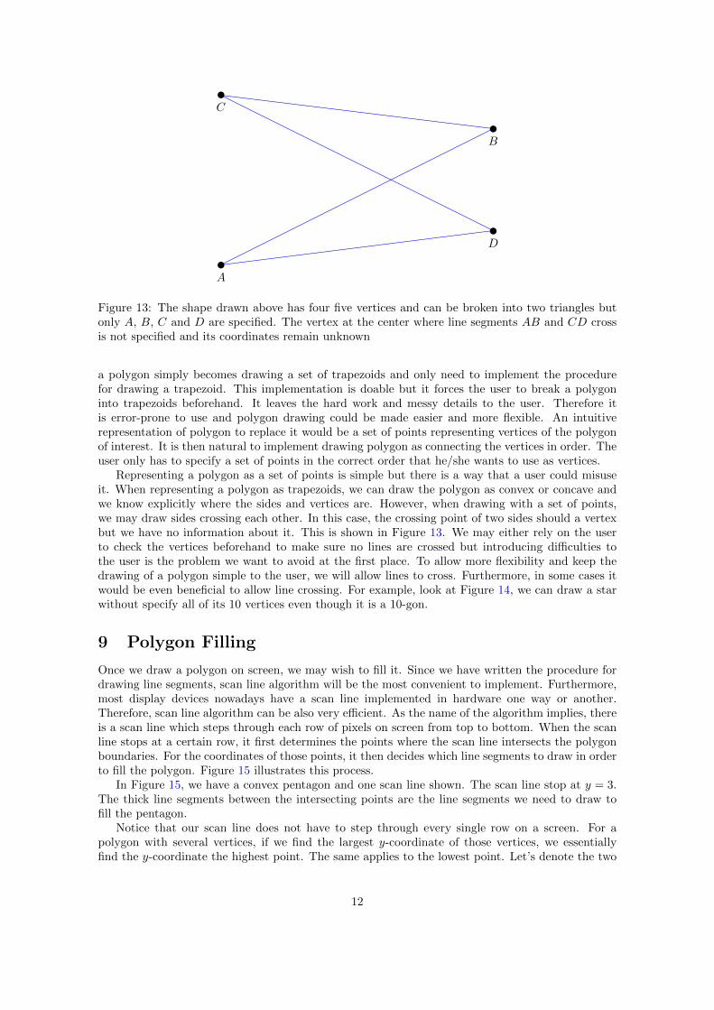
Figure 13: The shape drawn above has four five vertices and can be broken into two triangles butonly A, B, C and D are specified. The vertex at the center where line segments AB and CD crossis not specified and its coordinates remain unknown

a polygon simply becomes drawing a set of trapezoids and only need to implement the procedurefor drawing a trapezoid. This implementation is doable but it forces the user to break a polygoninto trapezoids beforehand. It leaves the hard work and messy details to the user. Therefore itis error-prone to use and polygon drawing could be made easier and more flexible. An intuitiverepresentation of polygon to replace it would be a set of points representing vertices of the polygonof interest. It is then natural to implement drawing polygon as connecting the vertices in order. Theuser only has to specify a set of points in the correct order that he/she wants to use as vertices.

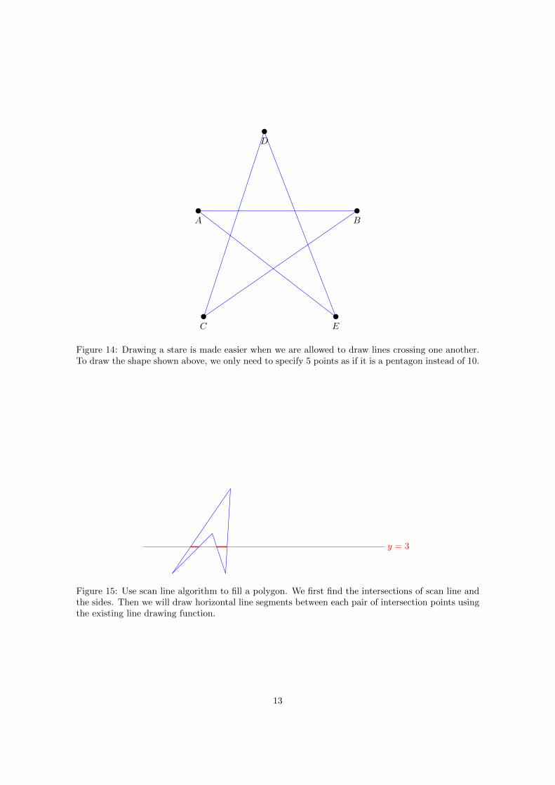
Representing a polygon as a set of points is simple but there is a way that a user could misuseit. When representing a polygon as trapezoids, we can draw the polygon as convex or concave andwe know explicitly where the sides and vertices are. However, when drawing with a set of points,we may draw sides crossing each other. In this case, the crossing point of two sides should a vertexbut we have no information about it. This is shown in Figure 13. We may either rely on the userto check the vertices beforehand to make sure no lines are crossed but introducing difficulties tothe user is the problem we want to avoid at the first place. To allow more flexibility and keep thedrawing of a polygon simple to the user, we will allow lines to cross. Furthermore, in some cases itwould be even beneficial to allow line crossing. For example, look at Figure 14, we can draw a starwithout specify all of its 10 vertices even though it is a 10-gon.

9 Polygon Filling

Once we draw a polygon on screen, we may wish to fill it. Since we have written the procedure fordrawing line segments, scan line algorithm will be the most convenient to implement. Furthermore,most display devices nowadays have a scan line implemented in hardware one way or another.Therefore, scan line algorithm can be also very efficient. As the name of the algorithm implies, thereis a scan line which steps through each row of pixels on screen from top to bottom. When the scanline stops at a certain row, it first determines the points where the scan line intersects the polygonboundaries. For the coordinates of those points, it then decides which line segments to draw in orderto fill the polygon. Figure 15 illustrates this process.

In Figure 15, we have a convex pentagon and one scan line shown. The scan line stop at y = 3.The thick line segments between the intersecting points are the line segments we need to draw tofill the pentagon.

Notice that our scan line does not have to step through every single row on a screen. For apolygon with several vertices, if we find the largest y-coordinate of those vertices, we essentiallyfind the y-coordinate the highest point. The same applies to the lowest point. Let’s denote the two

12

A

D

C

B

E

Figure 14: Drawing a stare is made easier when we are allowed to draw lines crossing one another.To draw the shape shown above, we only need to specify 5 points as if it is a pentagon instead of 10.

y = 3

Figure 15: Use scan line algorithm to fill a polygon. We first find the intersections of scan line andthe sides. Then we will draw horizontal line segments between each pair of intersection points usingthe existing line drawing function.

13

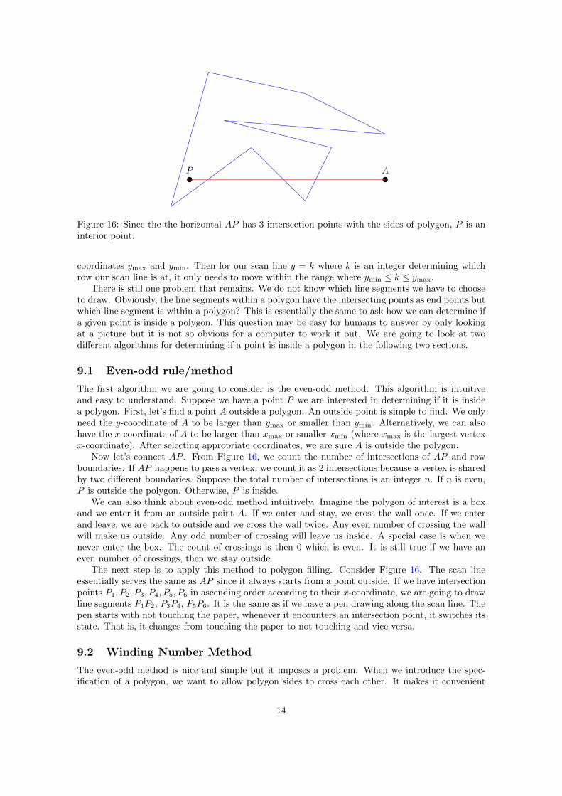
P A

Figure 16: Since the the horizontal AP has 3 intersection points with the sides of polygon, P is aninterior point.

coordinates ymax and ymin. Then for our scan line y = k where k is an integer determining whichrow our scan line is at, it only needs to move within the range where ymin ≤ k ≤ ymax.

There is still one problem that remains. We do not know which line segments we have to chooseto draw. Obviously, the line segments within a polygon have the intersecting points as end points butwhich line segment is within a polygon? This is essentially the same to ask how we can determine ifa given point is inside a polygon. This question may be easy for humans to answer by only lookingat a picture but it is not so obvious for a computer to work it out. We are going to look at twodifferent algorithms for determining if a point is inside a polygon in the following two sections.

9.1 Even-odd rule/method

The first algorithm we are going to consider is the even-odd method. This algorithm is intuitiveand easy to understand. Suppose we have a point P we are interested in determining if it is insidea polygon. First, let’s find a point A outside a polygon. An outside point is simple to find. We onlyneed the y-coordinate of A to be larger than ymax or smaller than ymin. Alternatively, we can alsohave the x-coordinate of A to be larger than xmax or smaller xmin (where xmax is the largest vertexx-coordinate). After selecting appropriate coordinates, we are sure A is outside the polygon.

Now let’s connect AP . From Figure 16, we count the number of intersections of AP and rowboundaries. If AP happens to pass a vertex, we count it as 2 intersections because a vertex is sharedby two different boundaries. Suppose the total number of intersections is an integer n. If n is even,P is outside the polygon. Otherwise, P is inside.

We can also think about even-odd method intuitively. Imagine the polygon of interest is a boxand we enter it from an outside point A. If we enter and stay, we cross the wall once. If we enterand leave, we are back to outside and we cross the wall twice. Any even number of crossing the wallwill make us outside. Any odd number of crossing will leave us inside. A special case is when wenever enter the box. The count of crossings is then 0 which is even. It is still true if we have aneven number of crossings, then we stay outside.

The next step is to apply this method to polygon filling. Consider Figure 16. The scan lineessentially serves the same as AP since it always starts from a point outside. If we have intersectionpoints P1, P2, P3, P4, P5, P6 in ascending order according to their x-coordinate, we are going to drawline segments P1P2, P3P4, P5P6. It is the same as if we have a pen drawing along the scan line. Thepen starts with not touching the paper, whenever it encounters an intersection point, it switches itsstate. That is, it changes from touching the paper to not touching and vice versa.

9.2 Winding Number Method

The even-odd method is nice and simple but it imposes a problem. When we introduce the spec-ification of a polygon, we want to allow polygon sides to cross each other. It makes it convenient

14

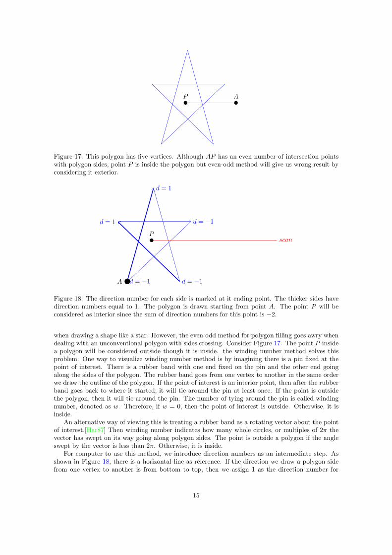
P A

Figure 17: This polygon has five vertices. Although AP has an even number of intersection pointswith polygon sides, point P is inside the polygon but even-odd method will give us wrong result byconsidering it exterior.

d = 1

d = −1

d = 1 d = −1

d = −1

scan

A

P

Figure 18: The direction number for each side is marked at it ending point. The thicker sides havedirection numbers equal to 1. The polygon is drawn starting from point A. The point P will beconsidered as interior since the sum of direction numbers for this point is −2.

when drawing a shape like a star. However, the even-odd method for polygon filling goes awry whendealing with an unconventional polygon with sides crossing. Consider Figure 17. The point P insidea polygon will be considered outside though it is inside. the winding number method solves thisproblem. One way to visualize winding number method is by imagining there is a pin fixed at thepoint of interest. There is a rubber band with one end fixed on the pin and the other end goingalong the sides of the polygon. The rubber band goes from one vertex to another in the same orderwe draw the outline of the polygon. If the point of interest is an interior point, then after the rubberband goes back to where it started, it will tie around the pin at least once. If the point is outsidethe polygon, then it will tie around the pin. The number of tying around the pin is called windingnumber, denoted as w. Therefore, if w = 0, then the point of interest is outside. Otherwise, it isinside.

An alternative way of viewing this is treating a rubber band as a rotating vector about the pointof interest.[Har87] Then winding number indicates how many whole circles, or multiples of 2π thevector has swept on its way going along polygon sides. The point is outside a polygon if the angleswept by the vector is less than 2π. Otherwise, it is inside.

For computer to use this method, we introduce direction numbers as an intermediate step. Asshown in Figure 18, there is a horizontal line as reference. If the direction we draw a polygon sidefrom one vertex to another is from bottom to top, then we assign 1 as the direction number for

15

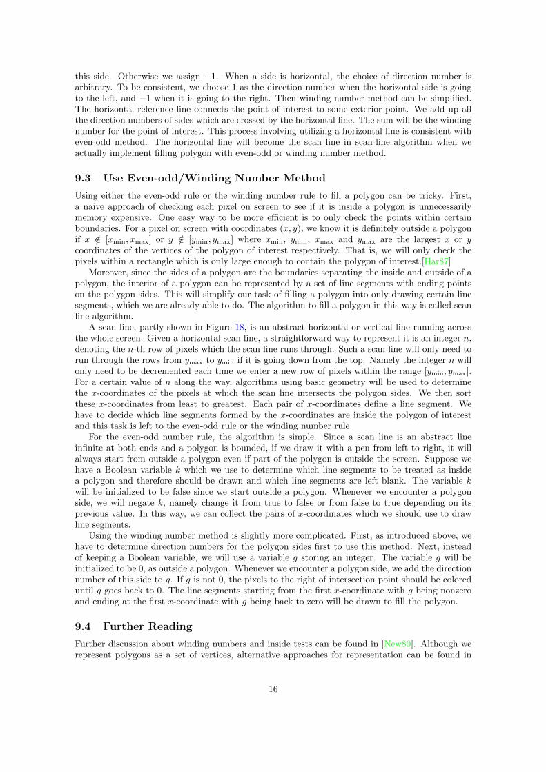
this side. Otherwise we assign −1. When a side is horizontal, the choice of direction number isarbitrary. To be consistent, we choose 1 as the direction number when the horizontal side is goingto the left, and −1 when it is going to the right. Then winding number method can be simplified.The horizontal reference line connects the point of interest to some exterior point. We add up allthe direction numbers of sides which are crossed by the horizontal line. The sum will be the windingnumber for the point of interest. This process involving utilizing a horizontal line is consistent witheven-odd method. The horizontal line will become the scan line in scan-line algorithm when weactually implement filling polygon with even-odd or winding number method.

9.3 Use Even-odd/Winding Number Method

Using either the even-odd rule or the winding number rule to fill a polygon can be tricky. First,a naive approach of checking each pixel on screen to see if it is inside a polygon is unnecessarilymemory expensive. One easy way to be more efficient is to only check the points within certainboundaries. For a pixel on screen with coordinates (x, y), we know it is definitely outside a polygonif x /∈ [xmin, xmax] or y /∈ [ymin, ymax] where xmin, ymin, xmax and ymax are the largest x or ycoordinates of the vertices of the polygon of interest respectively. That is, we will only check thepixels within a rectangle which is only large enough to contain the polygon of interest.[Har87]

Moreover, since the sides of a polygon are the boundaries separating the inside and outside of apolygon, the interior of a polygon can be represented by a set of line segments with ending pointson the polygon sides. This will simplify our task of filling a polygon into only drawing certain linesegments, which we are already able to do. The algorithm to fill a polygon in this way is called scanline algorithm.

A scan line, partly shown in Figure 18, is an abstract horizontal or vertical line running acrossthe whole screen. Given a horizontal scan line, a straightforward way to represent it is an integer n,denoting the n-th row of pixels which the scan line runs through. Such a scan line will only need torun through the rows from ymax to ymin if it is going down from the top. Namely the integer n willonly need to be decremented each time we enter a new row of pixels within the range [ymin, ymax].For a certain value of n along the way, algorithms using basic geometry will be used to determinethe x-coordinates of the pixels at which the scan line intersects the polygon sides. We then sortthese x-coordinates from least to greatest. Each pair of x-coordinates define a line segment. Wehave to decide which line segments formed by the x-coordinates are inside the polygon of interestand this task is left to the even-odd rule or the winding number rule.

For the even-odd number rule, the algorithm is simple. Since a scan line is an abstract lineinfinite at both ends and a polygon is bounded, if we draw it with a pen from left to right, it willalways start from outside a polygon even if part of the polygon is outside the screen. Suppose wehave a Boolean variable k which we use to determine which line segments to be treated as insidea polygon and therefore should be drawn and which line segments are left blank. The variable kwill be initialized to be false since we start outside a polygon. Whenever we encounter a polygonside, we will negate k, namely change it from true to false or from false to true depending on itsprevious value. In this way, we can collect the pairs of x-coordinates which we should use to drawline segments.

Using the winding number method is slightly more complicated. First, as introduced above, wehave to determine direction numbers for the polygon sides first to use this method. Next, insteadof keeping a Boolean variable, we will use a variable g storing an integer. The variable g will beinitialized to be 0, as outside a polygon. Whenever we encounter a polygon side, we add the directionnumber of this side to g. If g is not 0, the pixels to the right of intersection point should be coloreduntil g goes back to 0. The line segments starting from the first x-coordinate with g being nonzeroand ending at the first x-coordinate with g being back to zero will be drawn to fill the polygon.

9.4 Further Reading

Further discussion about winding numbers and inside tests can be found in [New80]. Although werepresent polygons as a set of vertices, alternative approaches for representation can be found in

16

[Bur77] and [Fra83]. We also mentioned we can represent a polygon by dividing it into trapezoidsor triangles. This technique is described in [Fou84] and [Gar78]

10 Transformation

Transformation is process of mapping a shape to another according to a well-defined rule. Transfor-mations such as rotating and scaling are common and we may want accomplish them in our graphicsprogram. For our program to be reusable, we want to be able to apply the same transformation todifferent shapes using the same sequence of code. Notice that any transformation of a shape can berepresented as mapping a point to a different point. Stretching a square to be twice as big will beas simple as mapping the coordinates of a vertex (x, y) to be (2x, 2y). Therefore, a universal way totransform different shapes is transforming the critical points, namely the points or other parametersthat define the shape of interest. In the case of a line segment, the critical points are its endingpoints. For a polygon, they are the vertices.

Furthermore, it will be more appealing if we can apply many different transformations to the sameshape while keeping our code running efficiently. We may also want our intended transformationsto be stored and applied all at once at the end therefore separating concerns. Another interestingquestion is whether there is a way we can build new complicated transformations from simpler ones.An intuitive way will be writing functions for different transformations and store the sequence oflabels of transformations we want to apply in an array. When we are ready to apply them, we checkthe label in order and invoke the corresponding function. This implementation is doable but it isnot efficient since the array consumes lots of memory when complicated transformation is applied.Since graphics is a frequent task, we need a more elegant solution. A universal way of representinga transformation is necessary. One of the common representations is matrix, which as we will seeshortly, is simple to implement and efficient for constructing complicated transformations.

10.1 Scaling Transformation

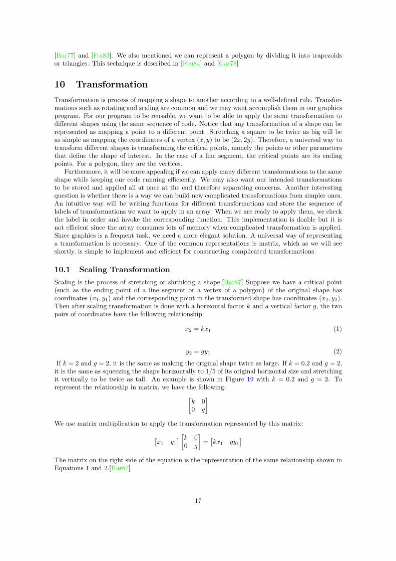
Scaling is the process of stretching or shrinking a shape.[Har87] Suppose we have a critical point(such as the ending point of a line segment or a vertex of a polygon) of the original shape hascoordinates (x1, y1) and the corresponding point in the transformed shape has coordinates (x2, y2).Then after scaling transformation is done with a horizontal factor k and a vertical factor g, the twopairs of coordinates have the following relationship:

x2 = kx1 (1)

y2 = gy1 (2)

If k = 2 and g = 2, it is the same as making the original shape twice as large. If k = 0.2 and g = 2,it is the same as squeezing the shape horizontally to 1/5 of its original horizontal size and stretchingit vertically to be twice as tall. An example is shown in Figure 19 with k = 0.2 and g = 2. Torepresent the relationship in matrix, we have the following:[

k 00 g

]We use matrix multiplication to apply the transformation represented by this matrix:

[x1 y1

] [k 00 g

]=[kx1 gy1

]The matrix on the right side of the equation is the representation of the same relationship shown inEquations 1 and 2.[Har87]

17

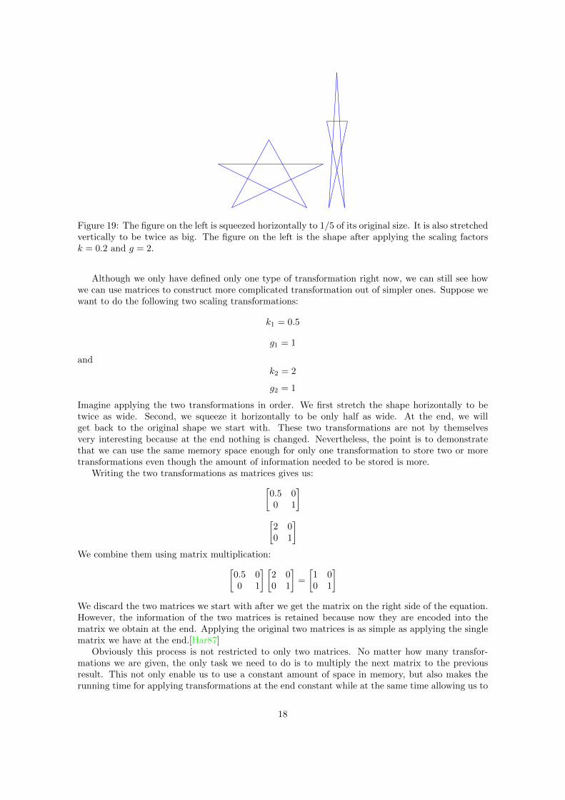
Figure 19: The figure on the left is squeezed horizontally to 1/5 of its original size. It is also stretchedvertically to be twice as big. The figure on the left is the shape after applying the scaling factorsk = 0.2 and g = 2.

Although we only have defined only one type of transformation right now, we can still see howwe can use matrices to construct more complicated transformation out of simpler ones. Suppose wewant to do the following two scaling transformations:

k1 = 0.5

g1 = 1

andk2 = 2

g2 = 1

Imagine applying the two transformations in order. We first stretch the shape horizontally to betwice as wide. Second, we squeeze it horizontally to be only half as wide. At the end, we willget back to the original shape we start with. These two transformations are not by themselvesvery interesting because at the end nothing is changed. Nevertheless, the point is to demonstratethat we can use the same memory space enough for only one transformation to store two or moretransformations even though the amount of information needed to be stored is more.

Writing the two transformations as matrices gives us:[0.5 00 1

][2 00 1

]We combine them using matrix multiplication:[

0.5 00 1

] [2 00 1

]=

[1 00 1

]We discard the two matrices we start with after we get the matrix on the right side of the equation.However, the information of the two matrices is retained because now they are encoded into thematrix we obtain at the end. Applying the original two matrices is as simple as applying the singlematrix we have at the end.[Har87]

Obviously this process is not restricted to only two matrices. No matter how many transfor-mations we are given, the only task we need to do is to multiply the next matrix to the previousresult. This not only enable us to use a constant amount of space in memory, but also makes therunning time for applying transformations at the end constant while at the same time allowing us to

18

dynamically adding any transformation as we like as long as the transformation can be representedas a matrix.

In the following subsections, we are going to survey other common transformations and illustratethem with examples. Also, we are going to introduce a slightly different way of using matrices torepresent transformations.

10.2 Rotation

If a point is represented in polar coordinates (r, θ), we only need to add a constant to θ to rotateit about the origin. However, since a screen is represented by a grid of pixels, we have to transferCartesian coordinates to polar coordinates, rotate, and transfer back. Luckily, basic geometry andtrigonometry have taught us how to do so.

Consider the point (1, 0). If we rotate it counterclockwise on the unit circle by an angle θ, itbecomes (cos θ, sin θ). That is, if we have a matrix[

a bc d

]to represent the transformation, we will have:

[1 0

] [a bc d

]=[a b

]which is the transformed coordinates [Har87]. Therefore, we get:

a = cos θ

b = sin θ

If we rotate the point (0, 1) counterclockwise by an angle θ, it becomes (− sin θ, cos θ) [Har87].Applying the procedure described above, we may conclude:

c = − sin θ

d = cos θ

Since every point on a plane can be broken down into the form u(1, 0) + v(0, 1), we are able toconstruct the rotation matrix to rotate a point counterclockwise about origin as [Har87]:[

cos θ sin θ− sin θ cos θ

]To construct a matrix to rotate clockwise is as simple as replacing θ with −θ. However, to rotateabout an arbitrary point instead of the origin requires more work to be done. Namely we need tobe able to perform translation.

10.3 Translation

So far we have used 2×2 matrix as our representation of transformation. However, 2×2 matrix doesnot serve the purpose of translation well. We can use a separate routine to deal with translation sinceit only involves adding constant factors to the coordinates, but doing this will violate our principleto represent different transformations in a similar fashion and be able to concatenate them to formmore complicated transformations. In other words, we want to stay homogeneous across differenttransformations. To account for translation, we use 3×3 matrix as our homogeneous representationinstead of 2× 2 matrix. We are going to see that 3× 3 matrix functions in the same way with thefollowing example.

19

Suppose we want to scale a point (x, y) with factors sx and sy. With 2× 2 matrix, we have:

[x y

] [sx 00 sy

]=[sxx syy

]Now we augment (x, y) with a dummy coordinate w. We call the new form of coordinates (x, y, w)homogeneous coordinates [Har87]. By applying a 3× 3 matrix, we have:

[x y w

] sx 0 00 sy 00 0 1

=[sxxw syyw w

]To get the same result as before, we simply set w to be 1. We then introduce the matrix used fortranslation: 1 0 0

0 1 0tx ty 1

Where tx and ty are the horizontal and vertical distances we want to translate. For the point (x, y),applying the matrix above we obtain (x+ tx, y + ty) which is the desired result for translation.

10.4 Rotation about an Arbitrary Point

Rotation about an arbitrary point is actually three transformations in sequence [Har87]. Suppose werotate about the point (xc, yc) and the point to be rotated is (x, y). We first translate (x, y) in thedirection (−xc,−yc). Second, we rotate about the origin. Third, we translate back by translatingwith factors (xc, yc). For the user’s convenience, we want to construct a single matrix. This is as easyas doing some simple matrix multiplication operations since we have the necessary transformationsall encoded in 3× 3 square matrix. 1 0 0

0 1 0−xc −yc 1

cos θ sin θ 0− sin θ cos θ 0

0 0 1

1 0 00 1 0xc yc 1

=

cos θ sin θ 0− sin θ cos θ 0

−xc cos θ + yc sin θ + xc −xc sin θ − yc cos θ + yc 1

Again, this is for counterclockwise rotation, but how to rotate clockwise is as simple as only replacingθ with −θ.

10.5 Reflection

Reflection is another common task we want to accomplish. Matrices below are the representationsfor different reflections. For simplicity we have omitted the unused part of our homogeneous 3 × 3matrix representations and only present them as 2 × 2 matrices. A reader can re-construct thehomogeneous representation by simply adding the omitted part.

Reflection about the y axis: [−1 00 1

]Reflection about the x axis: [

1 00 −1

]Reflection about the origin: [

−1 00 −1

]

20

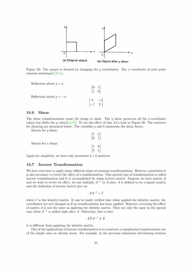
Figure 20: The square is sheared by changing the y coordinates. The x coordinate of each pointremains unchanged [Tuta].

Reflection about y = x: [0 11 0

]Reflection about y = −x: [

0 −1−1 0

]

10.6 Shear

The shear transformations cause the image to slant. The y shear preserves all the x-coordinatevalues but shifts the y value[Har87]. To see the effect of this, let’s look at Figure 20. The matricesfor shearing are presented below. The variables a and b represents the shear factor.

Matrix for y shear: [1 a0 1

]Matrix for x shear: [

1 0b 1

]Again for simplicity, we have only presented 2× 2 matrices.

10.7 Inverse Transformation

We have seen how to apply many different types of common transformations. However, sometimes itis also necessary to revert the effect of a transformation. This special type of transformation is calledinverse transformation and it is accomplished by using inverse matrix. Suppose we have matrix Aand we wish to revert its effect, we can multiply A−1 to A since A is defined to be a square matrixand the definition of inverse matrix give us:

AA−1 = I

where I is the identity matrix. It can be easily verified that when applied the identity matrix, thecoordinates are not changed as if no transformation has been applied. However, reverting the effectof matrix A is not the same as applying the identity matrix. They are only the same in the specialcase when A−1 is added right after A. Otherwise, due to fact:

AXA−1 6= X

it is different from applying the identity matrix.One of the applications of inverse transformation is to construct a complicated transformation out

of the simple ones we already know. For example, in the previous subsection introducing rotation

21

about an arbitrary point, we first translate the coordinates, then rotate about origin and finallytranslate back. The third matrix for translating back is actually the inverse matrix of the first one.We are going to see more examples like this in the section for drawing 3D shapes.

10.8 Further Reading

Although using matrix to represent transformations is handy and better than a naive approach weproposed in the beginning, it is definitely not the only way to transform a shape. Other techniquesmay be found in [Bra80].

11 Re-visting Display File

So far we have introduced the ways for drawing a line segment, drawing and filling a polygon,and applying transformations. We may want to put together all the procedures into a single pieceof software while following software engineering principles. We have used display file to store thecommands for drawing line segments and have the drawer object to execute them. The routines fordrawing polygons are similar to those for line segments. There will be absolute and relative versionsof routines for drawing polygons. However, instead of passing coordinates of vertices to the routines,we will have the user store the coordinates in two arrays and then pass the arrays. One of the arrayswill be storing the x-coordinates of all vertices. The other will store the y-coordinates. The lengthsof both arrays should be the same as the number of sides. And if the two arrays have differentlengths, an error will be thrown. Furthermore, we may have a routine to automatically find out thenumber of sides from the length of either array but we may also have the user to specify it. Again,if the number of sides specified by user does not match with either array, an error should be thrown.

When the routine for drawing polygon is called, it is not clear about what data it should putinto the display file. Remember in the case of line segments, we have to tell the display file the x,y coordinates and the opcode. Since we have not used any opcode larger than 2 and the minimumvalid number of sides of a polygon is 3, we will use any opcode larger than 3 to represent the numberof sides. If we want to add commands for other shapes such as a circle or a curve, we may usenegative numbers as opcodes. As for the values of x and y, we will use them to store the coordinatesof the first vertex. This command will be called polygon command thereafter.

However, after doing this, we run out of space for storing necessary information for drawing apolygon. If the polgyon has n vertices, we have no place to store the coordinates for the remainingn−1 vertices. Also, we have no way to have the display file to tell the drawer object to fill a polygon orleave it unfilled. For the first problem, we simply add a sequence of line segment drawing commandsto draw polygon sides following the polygon command. In this way, the polygon command will beinterpreted as a move command to move the pen to the position of the first vertex. Also, the opcodeof the polygon command will be used to determine how many line segment drawing commands thereare for the polygon. For a polygon with n vertices, we need to draw n sides. Therefore, we put nline segment drawing commands in order following the polygon command. The x and y slots of thefirst n−1 line segment drawing commands will store the corresponding coordinates of the remainingn− 1 vertices. The slots of the last command will store the coordinates of the first vertex as we donot want to leave a gap. When combined, the n+ 1 new commands introduced so far will enable usto draw the outline of a polygon on screen.

As for letting the user choose whether a polygon should be filled, instead of inventing a newcommand, we will simply use a Boolean variable to indicate the choice. Also, we will includeanother set of variables to indicate the intensity, the color and other parameters with which we useto fill the polygon. If the task of graphics is implemented in hardware, those variables will insteadbecome registers.

We may wish to add the functionality of transformation now but any implementation we comeup with may not be ideal. We may wish to apply different transformations to different shapes.Remember there is only one display file in memory and we have no way to distinguish one shapefrom another. Therefore for any transformation we apply, it is applied to the whole screen. Moreover,the Boolean variable we introduced above to indicate if a polygon should be filled will not enable

22

us to fill some polygons while leaving the others blank. To be able to do so also requires a way todistinguish different shapes. We will be dividing the display file into different segments and the wayof dividing will be introduced in the next section.

12 Segment

Segments are extensively used in graphics. Consider the animations in a video game. An objectmay be moving from right to left while the background remains static. A sequence of translationmatrices will be applied to the object alone repeatedly to make it look like moving. In the displayfile, we will have a segment for this object while having another for the background. The programshould then only apply transformations to the segment of the object. Since display file is supposedto only contain drawing instructions, to separate concerns, we will implement segments and storethe necessary information in a separate table called segment table. The table will be a fixed set ofarrays. The indices of the arrays will be the names for segments. One array called “start” shouldstore the index which indicates where a segment starts in a display file. Another array called “offset”will store the number of instructions in display file that belong to the segment. Suppose for segmenti, the integers stored in the start and the offset arrays are a and k. Then all of the instructions withindices from a to a+ k − 1 will belong to segment i.

Other arrays will store information for transformation and filling parameters. For example, onearray will store the angles for rotation transformation and another pair of arrays will store the twoscaling factors. However, some operating systems or graphic cards may not automatically initializethe slots of arrays with 0’s. If a certain transformation is not specified for a segment, random junkmay trick the program into thinking there is a transformation to apply. The way to deal with thisis to initialize the slots with some default values but we should be careful not to make them all 0’ssince different transformations require different default values. For rotation, the default value willbe 0 and for scaling, the value will be 1.

Part of a segment table is shown below

index start offset y tx ty theta sx sy0 0 30 25 0 0 0 1 11 30 4 40 1 14 0 1 12 34 10 20 0 0 π/2 2 2

We have three segments in the segment table above. The transformation factors for the firstsegment forms an identity matrix. Therefore it is not transformed and may serve as the background.The second segment will be translated by 1 pixel to the right and 14 pixels to the top. The thirdwill be rotated counterclockwise by an angle π/2 and then made twice as large as before. However,the third segment poses a problem. If the user wants a segment to be transformed in multiple ways,the order of applying transformation is ambiguous. In the case of the third segment, we simplyassume there is a fixed order of transformations to be applied, but this requirement severely limitsthe number of the user’s choices. To solve this, we may have the segment table to directly storethe matrices to be applied, but for the simplicity of implementation, we are only going to use thesimpler but less useful version of segment table.

We should also add routines for the user to use our segment table. Those routines will includesegment creation, retrieval, modification and deletion as well as routines for storing transformationand filling parameters. Since those routines are simple to implement, we will not include the detailshere. Although not required, we can also allow the user to specify nested segments. This can beimplemented by simply relaxing the constraints for the values of start and offset of a segment.

13 Windowing and Clipping

Windowing and Clipping are common tasks in graphics programming. Windowing is the procedureof putting arbitrary boundaries on the figure of interest. We then select part of the figure andre-locate it. Clipping compliments windowing. After part of a figure is selected, parts of the figure

23

outside the window should be removed. This will reduce the computing time and resources requiredto render the figure.

13.1 Windowing

Before diving into the specifics of windowing, there are two concepts essential to this task. Fist,an object model is the model with which we model the figure of interest. For example, we mayspecify a figure in object model with units such as centimeters, kilometers or even light years. Aview model is the coordinate system we use on an actual screen or frame buffer where the units suchas centimeters do not make sense. The only unit we are going to use in a view model is the pixel. Ifwe normalize the width and length of a screen such that the length of a line segment is representedas the ratio of width or length, it is then possible to specify the coordinates of a point with numberssmaller than 1. For example, on a screen 200-pixels wide and 100-pixels high, using pixel as the unit,if the point P has coordinates (50, 50), P can be represented in a normalized coordinate system as(0.25, 0.5).

A window is a selected region of the object model of a figure. For example, if we want to drawa house on screen, we may select the front door of the house as our window. For simplicity, we willonly discuss window of a rectangular shape and currently we are only interested in having 2D figuresin the object model. Also, since we want our implemented software to remain general, figure in theobject model will also be specified with normalized coordinates. An actual application to a specificarea may then be required to have a routine to convert the real-world units such as centimeters andlight years to the normalized coordinates.

A viewport is a selected region of the view model. It determines where and how we want todisplay the selected part of a figure in object model. Again, for simplicity, we will only deal withrectangular viewport. Therefore, our task for windowing can be divided into three parts. First, wehave the user select the desired window on the figure. Second, we have the user specify the desiredviewport. Third, we put the selected part in the viewport. The first two steps for windowing aresimple to implement. We only need to write routines to store the window and viewport boundaries.We will use symbols wr, wl, wt, wb to represent the right, left, top and bottom boundaries of thewindow and vr, vl, vt, vb for the boundaries of viewport respectively. The third step of windowingmight seem a little daunting and complicated but in fact, it is really only a transformation in disguise.

13.2 Windowing Transformation

Windowing transformation is the combination of a sequence of simpler transformations. We aregoing to use translation and scaling to achieve the construction. First, we move the lower-left cornerof window to the origin. Second, we move it to the corresponding viewport corner location. Whenthe window is at the origin, we perform some necessary scaling. The reason to do the scaling atorigin is that we can avoid disturbing the corner’s position. Therefore, we will have three matricesand we are going to combine them using matrix multiplication. 1 0 0

0 1 0−wl −wb 1

vr−vlwr−wl

0 0

0 vt−vbwt−wb

0

0 0 1

1 0 00 1 0vl vb 1

=

vr−vlwr−wl

0 0

0 vt−vbwt−wb

0

vl − wlvr−vlwr−wl

vb − wbvt−vbwt−wb

1

13.3 Clipping

Without clipping to remove the parts that a user is not interested in, our routine for windowing isonly scaling and translating transformations combined. Clipping is what will make the figure looklike that it has been selected and the user is looking through a real window. First, we will explore

24

Figure 21: The positive bit represents the state of a vertex being outside a boundary. The negativebit represents that in reference to a particular boundary, the vertex in question is considered inside[Wha].

a simple yet efficient algorithm for clipping line segments. Later, another algorithm for clippingpolygon will be introduced.

13.3.1 The Cohen-Sutherland Outcode Line Clipping Algorithm

This algorithm was first developed by Danny Cohen and Ivan Sutherland in 1967. Although thealgorithm was introduced in an early era of computer graphics, its simplicity and efficiency allow itto be still widely used and become the foundations of other more efficient line-clipping algorithms.Information about the other algorithms that improve upon Cohen-Sutherland Outcode Algorithmcan be found in the Further Reading Section. The Outcode Algorithm makes use of a type ofinformation storage unit called outcode. Outcode is a data structure holding four bits. Each linesegment will have two outcodes. One end point of a line segment will correspond to one outcode.For a line segment l with end points (x1, y1) and (x2, y2). The end points have outcodes c1 and c2respectively. If y1 > wt, then the first bit of the outcode c1 is assigned value 1. Otherwise the firstbit is assigned 0. If y1 < wb, then the second bit is assigned 1. Otherwise it is assigned 0. Theprocess goes on for x1 testing against wl and wr. The third bit corresponds to wr and the fourth bitis for wl. That is, if the end point is outside a boundary, the corresponding bit for that boundary isassigned 1 and otherwise it is assigned 0. We repeat the same process with end points (x2, y2) andits outcode c1. At the end, we will have a pair of outcodes for a line segment. If both line segmentsare 0000, then the line segment lies inside the window. If the line segment is not inside, we take alogical “AND” of the two outcodes. If the result is nonzero, the segment lies completely outside,since at least one bit position in the two outcodes have both 1. That is, both of the end points lieat the outside of a boundary line. If the result of “AND” operation is zero, we determine which sidehas been crossed, find the point of intersection and repeat the process for clipping until we have aclipped segment which lies inside the window. In this algorithm, we essentially divide the plane intonew regions. This is illustrated in Figure 21

13.4 The Sutherland-Hodgman Polygon Clipping Algorithm

The Sutherland-Hodgman Polygon Clipping Algorithm is one of earliest polygon clipping algorithms.It can clip general polygons including normal convex, concave and self intersecting polygons. How-ever, the only limitation it has is that the window for clipping has to be concave. Although it hasbeen replaced by some more general and efficient algorithms such as Vatti clipping algorithm, itsfame for being easily understandable still makes it one of the popular choices. To learn about themore general Vatti algorithm, please refer to the Further Reading section.

Sutherland-Hodgman algorithm starts with a list of polygon sides. For each window boundary, itclips all sides against that boundary. Suppose we have a rectangular window and the left boundaryis x = 1. Then for each vertex (x0, y0), it is simple to test if it lies on the right or left side of theleft boundary. If x0 > 1, then the vertex is on the right side. Otherwise, it is on the left side. Wealso call the left side of a left boundary the outside of this boundary as any point in this region isdefinitely outside the window. We call the right side of a left boundary the inside of this boundary

25

as any point in this region may be located inside the window. The similar classification applies tothe other three boundaries.

After knowing how to do inside tests, before we dive into the details of the algorithm, we have tochange our notion about what a polygon side represents. Instead of only considering a polygon sideas a line segment, we are going to also consider it as a vector. That is, in the following paragraph,we are going to consider it as a line segment with direction. The ending point of the vector of apolygon side will be the starting point of the vector of the next side.

In Sutherland-Hodgman algorithm, for each polygon side being clipped against a particularwindow boundary, we first determine which vertex lies inside or outside of this boundary. If bothvertices lie inside the boundary, we the coordinates of both points. If both vertices are outside, wediscard them and move to the next side. If one is inside and another is outside, the polygon sidemust cross the boundary line. We then determine the point of intersection between the side and theboundary. After that, we save the coordinates of the point of the intersection and the vertex insidethe boundary. Suppose we have clipped the first polygon side and it does not lie completely outsidethe boundary. That is, for this polygon side, we have saved coordinates of two points in memory. Forthe next polygon side we consider against the same boundary, we repeat the same procedure. If bothvertices are outside, we discard them and move on to the next side until we encounter a side whichhas at least one vertex inside the boundary. We then retrieve the previous two points we saved.Since each polygon side corresponds to a vector, each clipped side also corresponds to a vector. Wedenote the ending point of the vector of the previous clipped side as p1 and the starting point of thevector of the current clipped side as p2. We then connect them using a move command. That is, inthe display file, we move from point p1 to p2. For each move command we add, we essentially addone more polygon side. However the polygon side is invisible since it is only a portion of the windowboundary. We continue the process with all sides of a polygon with this particular boundary. Afterthat, we iterate through the remaining boundaries. At the end, we will some line drawing commandsand move commands which enable the display file to draw the clipped polygon correctly.

If all the sides lie outside of any of the window boundaries, then no commands will be entered inthe display file. If at least one boundary crosses any of the boundaries, another side will have to crossthe same boundary because a polygon is closed without gaps on its sides. Therefore the algorithmdescribed above is consistent with any polygons. We either have a clipped polygon (including apolygon lies completely inside) or a polygon lying completely outside. In either case, the result isdesired. We either have polygon with zero or more invisible sides or polygon that is never drawn.

13.5 Limitations of Sutherland-Hodgman Algorithm

As mentioned in the beginning of the previous subsection, Sutherland-Hodgman Algorithm hascertain limitations. One of them is that the window has to be convex. To see why the windowcannot have other shapes such as a concave or self-intersecting polygon, recall inside testing againsteach window boundary is an essential part of the algorithm. When we have a window of convexshape, when a vertex is outside of any boundary line, we are sure it is outside of the window.However, when we have a window of concave shape, when a vertex is outside of a boundary line, itmight be the case that the vertex is actually inside the window. Therefore, the inside test againsteach boundary of a window of concave shape is not always consistent. We will also be in the samesituation if we use a window shaped as a self-intersecting polygon.

13.6 Further Reading

Although Sutherland-Hodgman Clipping Algorithm has the limitation that the window has to beconvex, it is still a popular choice because in most cases we only need a concave window. In the caseswhen using a window of non-concave shape is necessary, Vatti algorithm will be a better choice. Tolearn about this algorithm, refer to [Vat92]

26

14 3D Representation and Transformation

Until now we have considered how to draw 2D shapes on screen. Although for some tasks whatwe have developed is enough, it is certainly more interesting if we may not only be able to put flatshapes but also 3D ones on screen. The way of doing this is actually much easier than what most ofus might have thought. It turns out that drawing 3D shapes is as simple as applying transformationson 2D shapes. The only problem we need to solve is then what the specific transformations we needto construct. However, before we keep ourselves busy constructing those special transformations,we have to know first how to represent 3D shape in an abstract and manageable way in computermemory.

14.0.1 3D Representation

In the 3D world, since there are three different dimensions, we need at least 3 parameters to representa 3D object. The most convenient form of representation is Cartesian coordinates as we used in 2Dworld. In some other situations, we might use other systems of coordinates to represent a point, butthe conversion from most of the other systems to Cartesian coordinates is well-known and simple toimplement. Here, we will stick with Cartesian coordinates in our discussion.

A point in 3D world can be represented as (x, y, z). A line can be represented with a point onthe line and vector indicating its direction. It is not easy and in most cases not convenient to deriveand use a single equation of a line in 3D. Therefore, we will exclusively use parametric form of aline. The parametric representation of a line also makes it easy to specify a line segment as weonly need to specify the range of the parametric variable. For polygons in 3D, we restrict ourselvesin only considering a polygon with all of its sides being on the same plane. That is, although ourrepresentation of a polygon as an array of vertices makes it possible to have the sides on differentplanes, we discard those radicals and only consider conventional polygons.

14.1 Transformation in 3D

Trying to represent and make use of 3D figures essentially introduce two different worlds, or twochunks of memory space we interpret differently. The first is the 3D world. It models the actualworld we live without reference to time. The second is the 2D world. It models the plane of computeror TV screen where we actually can see what our figures are like. It would be ideal if we can havea 3D screen and simply put our 3D figures on the screen. However, most screens on market areflat. Therefore, our 3D figures remain as abstract representation and to view them, we have to finda systematic way to map them into the 2D world. We will call the 3D world our data model andsimply refer 2D world as screen or the plane of a screen.

Before we see the actual ways of mapping from data model to screen, we need to extend ournotions of transformations from 2D to 3D. The transformations we are going to introduce are essentialin understanding and constructing the mappings.

14.2 Scaling and Translation

Same as in 2D, scaling refers to squeezing and stretching and translation refers to movement in spacewithout changing shape. However, instead of two coordinates, we now have three coordinates to workon, so instead of squeezing, stretching or moving in two possible directions, we will be squeezing,stretching or moving our figure in three possible directions. Also, the addition of z-coordinaterequires us to use 4 matrix.

The matrix for scaling is given below where sx, sy, sz refer to the x, y, z scaling factors respec-tively.

sx 0 0 00 sy 0 00 0 sz 00 0 0 1

27

Let’s apply the matrix to an arbitrary point (x, y, z) to verify it produces desired result. Again, wehave a dummy coordinate w0 to allow the use of 4× 4 matrix in order to make room for translationfactors.

[x y z w0

] sx 0 0 00 sy 0 00 0 sz 00 0 0 1

=[sxx syy szz w0

]The matrix for translation is also similar to its counterpart in 2D. Below, we have tx, ty and tz astranslation factors for each coordinate respectively.

1 0 0 00 1 0 00 0 1 0tx ty tz 1

Applying it gives us:

[x y z w0

] 1 0 0 00 1 0 00 0 1 0tx ty tz 1

=[x+ w0tx y + w0ty z + w0tz w0

]

which is as expected after assigning w0 with value 1.

14.3 Rotation about Axis

Rotation in 3D is a little more different than in 2D. Unlike in 2D, rotating about a point in 3D isnonsense since the number of paths of rotation is infinite. The point can end up being anywhere onthe surface of a particular sphere. The only sensible form of rotation is rotation about a line. Theline can x-, y-, z-axis or any other arbitrary line. In this section, we consider rotation about thethree axes. In the next section, we will explore the way of rotating about an arbitrary line based onsimpler transformations such as translation and rotation about an axis introduced in the previousand current sections.

14.3.1 Rotation about z-Axis

Rotation about z-axis is particularly easy to understand. Since the point of interest is moving aroundthe z-axis, its z-coordinate remains constant while the other two coordinates keep changing. It isas if we are moving in the xy plane which has exactly the same representation with a screen or the2D world. Therefore, the only thing we need to do is simply inserting the components of our 2× 2matrix for rotation about origin into 4× 4 identity matrix. The matrix is given below. The angle ofrotation is represented by symbol θ and the direction of rotation is counterclockwise.

cos θ sin θ 0 0− sin θ cos θ 0 0

0 0 1 00 0 0 1

Verification for the validity for this matrix to produce the coordinates of the rotated point is similarto previous matrices and not hard to do, so we will not cover the details here.

14.3.2 Rotation about x-Axis

Rotation about x-axis is similar to that of z-axis. We simply relabel the three axes and treat x-axisas if it is the z-axis. And we treat the other two axes as the x- and y- axes. Then the rotation

28

about x-axis is identical as the rotation about z-axis. Again, the construction of the matrix is simplyreplacing some components in the 4× 4 identity matrix and the matrix is given below.

1 0 0 00 cos θ sin θ 00 − sin θ cos θ 00 0 0 1

Verification for this matrix is left to the reader as exercise.

14.3.3 Rotation about y-Axis

Constructing the matrix for rotation about y-axis is also achieved by relabling the axes. We will notgo into details here as the process is similar. The matrix for rotation about y-axis is given below.

cos θ 0 − sin θ 00 1 0 0

sin θ 0 cos θ 00 0 0 1

14.4 Rotation about an Arbitrary Line

Remember when we were constructing matrices for rotation about an arbitrary point in 2D world, wefirst translate the center of rotation to the origin, then rotate about the origin and finally translateback. The process of constructing matrix for rotation about an arbitrary line is similar though moredetails have to be taken care of. We first transform the axis (line around which the rotation is done,not the x-, y-, or z- axes) to some position or orientation where we know how to rotate about theaxis. Next, we rotate about the axis and finally use inverse transformations to bring the axis backto its original position and orientation.

Thus, the problem resides in where we know how to rotate about a line already. So far the onlylines around which we are able to rotate a point are the three axes of the coordinate system. Theseare what we will use to build the matrix for rotation about an arbitrary line.

Suppose the axis is specified by the following equations:

x = Au+ x1

y = Bu+ y1

z = Cu+ z1

where [A,B,C] is the vector indicating the direction of the line. From the equations, wer are sure(x1, y1, z1) is on the line. Therefore we translate the axis by the factors −x1, −y1 and −z1 such thatthe line passes through the origin. The matrix for doing this is given below and denoted as T :

T =

1 0 0 00 1 0 00 0 1 0−x1 −y1 −z1 1

Since eventually we want to translate back to its original position, we will also make its inversematrix:

T−1 =

1 0 0 00 1 0 00 0 1 0x1 y1 z1 1

The next step is trying to rotate the axis of rotation around x-axis until the axis of rotations is inxz-plane. However, we do not how much the rotation angle about x-axis is. To figure that out,imagine we make a parallel projection of the line onto the yz-plane. The direction of projection is

29

parallel to x-axis. Since the direction vector of the line is [A,B,C] and we have moved it such thatit passes origin, the line segment L1 from point (0, 0, 0) to (A,B,C) is on the axis of rotation. Theprojected point of (A,B,C) will have coordinates (0, B, C). Denote the line segment from origin to(0, B,C) as L2. The length of this segment is then

V =√B2 + C2

When we rotate L1 around x-axis, segment L2 is also rotated. The angles of each rotation are equal.That is, to find out the amount L1 needs to rotate about x-axis to land in xz-plane, we can insteadfind the angle of rotation of L2. Moreover, we actually do not need to know how much this angleis. Since in all the rotation matrices, only the cosine and sine of an angle is used, we only need toobtain those two values instead of the actual angle.

Basic trigonometry in yz-plane give us:

sin I =B

V

cos I =C

V

where I is amount that L2 needs to rotate about the origin in yz-plane.Fortunately, each of the three values B, C and V is known beforehand, and the matrix Rx is as

follows:

Rx =

1 0 0 00 C/V B/V 00 −B/V C/V 00 0 0 1

and we also need the inverse matrix:

Rx−1 =

1 0 0 00 C/V −B/V 00 B/V C/V 00 0 0 1

Suppose the final target matrix we want to achieve eventually isM . Up until now, we haveM = TRx.This temporary value of M is the same as saying our axis of rotation is lying in the xz-plane. Thenext step is rotating about y-axis so that it overlaps z-axis. Then the rotation about the line is thesame as rotation about z-axis, which is easily achievable.

Denote the line segment in xz-plane after rotating L1 about x-axis as L3. Its length N does notchange after applying T and Rx. Therefore,

N =√A2 +B2 + C2

If we have to rotate about y-axis for angle J , then,

sin J =A

N

cos J =V

L

and the matrix Ry for such a rotation will be:

Ry =

V/N 0 A/N 0

0 1 0 0−A/N 0 V/N 0

0 0 0 1

30

The inverse matrix is,

Ry−1 =

V/N 0 −A/N 0

0 1 0 0A/N 0 V/N 0

0 0 0 1

Finally, we are going to rotate about z-axis for angle θ. Since now the axis of rotation is the sameas z-axis, rotating about z-axis is the same as rotating about the line. The matrix Rz for this is,

Rz =

cos θ sin θ 0 0− sin θ cos θ 0 0

0 0 1 00 0 0 1

Notice that we do not need the inverse of matrix Rz.

Putting all the matrices we have developed so far in this section, we can finally obtain the correctmatrix M for rotation about an arbitrary line:

M = TRxRyRzRy−1Rx

−1T−1

15 Projection from 3D to 2D

Equipped with the tools of 3D transformation, finally we are going to introduce how to map a3D object onto a 2D screen. This process of mapping is called projection. Intuitively projectionmight sound complicated but actually, surprisingly enough, projection is as simple as a special typeof projection. Once we know the matrices for projection, what is left to do is simply doing somematrix algebra and get the coordinates for drawing on screen.

Since on a flat screen we only need two numbers to specify the position of a point and in 3Dmodel, we use three numbers to specify a point, some of us might guess using a 3×2 matrix will sufficethe purpose of projection. However, although this approach is doable, using a non-square matrixintroduces problem when we want to combine transformations as matrix multiplication requires thenumber of columns in the previous matrix being equal to the number of rows in the next. Also, sometransformations like translation will pose problems as its matrix is not compatible with a matrixhaving dimensions other than 4× 4. And translation matrix is certainly used in the construction ofcertain type of projection. Therefore, we will continue using 4× 4 matrices as our representation oftransformation and projection and we will augment the coordinates in 2D and 3D worlds to havedimension 4. That is, in 3D, we keep using the coordinates with dummy coordinate w0. And in 2d,we use (x, y, z, w0) as the coordinates even though z may not be used.

Below is a brief introduction of the two major types of projection.A parallel projection is formed by extending parallel lines from each vertex on the 3D object

until they intersect the screen. The point of intersection is the projection of the vertex. We connectthe projected vertices by line segments which corresponds to original object [Har87]. One commonuse of parallel projection is found in engineering field such as a three-view drawing shown in Figure22.

An alternative projection is a perspective projection. In a perspective projection, the furtheraway an object is from the viewer, the smaller it appears. This provides the viewer a depth cue.The lines of projection are not parallel. Instead, they all converge at a single point called the centerof projection. It is the intersections of these converging lines with the plane of the screen thatdetermine the projected image [Har87]. A close analogy of perspective projection is human eyes orcamera which operate under the same mathematical model. An illustration of this type of projectioncan be found in Figure 23.

15.1 Parallel Projection as Transformation

As mentioned above, same with transformation, projection can be represented simply as a matrix.In this section, we explore how to construct the matrix for parallel projection.

31

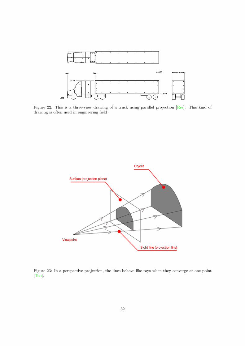
Figure 22: This is a three-view drawing of a truck using parallel projection [Res]. This kind ofdrawing is often used in engineering field

Figure 23: In a perspective projection, the lines behave like rays when they converge at one point[Tou].

32

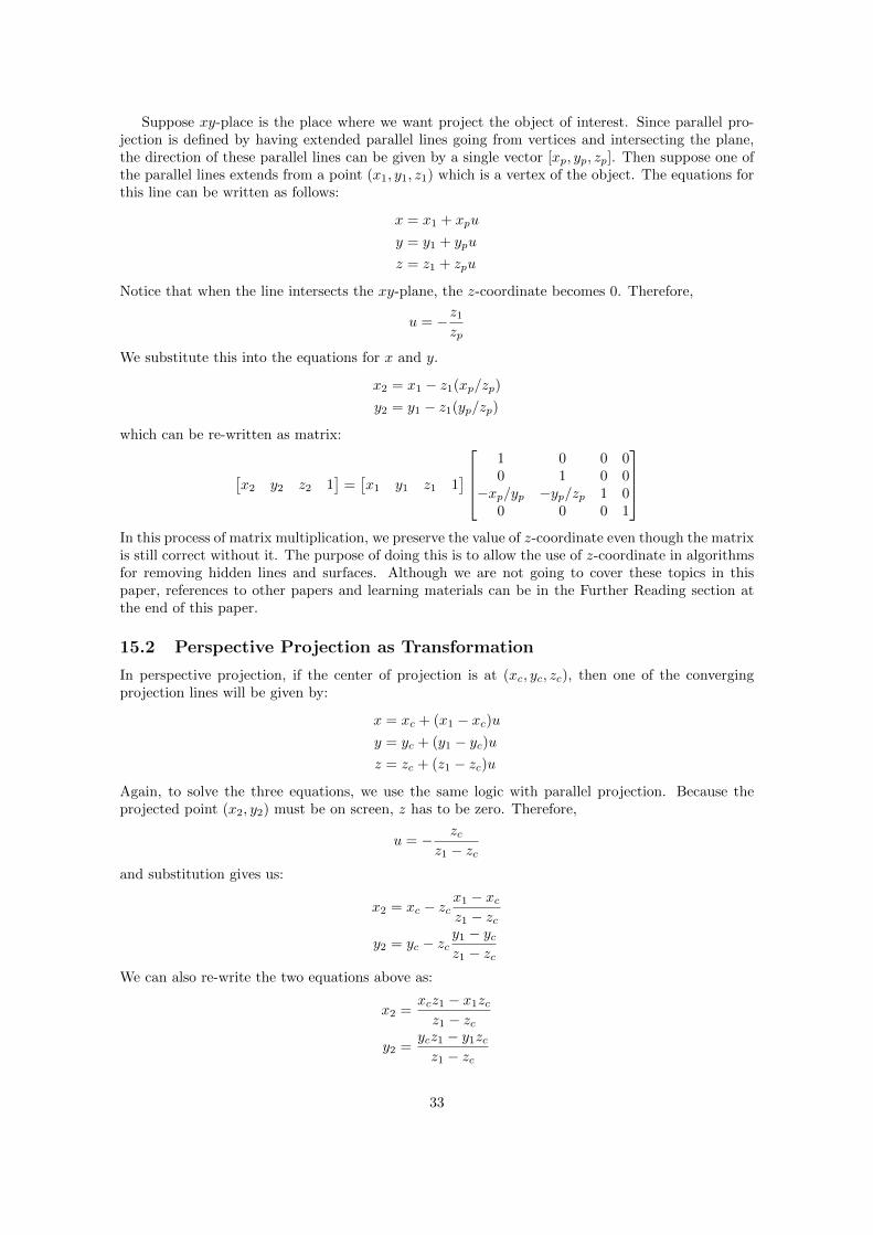
Suppose xy-place is the place where we want project the object of interest. Since parallel pro-jection is defined by having extended parallel lines going from vertices and intersecting the plane,the direction of these parallel lines can be given by a single vector [xp, yp, zp]. Then suppose one ofthe parallel lines extends from a point (x1, y1, z1) which is a vertex of the object. The equations forthis line can be written as follows:

x = x1 + xpu

y = y1 + ypu

z = z1 + zpu

Notice that when the line intersects the xy-plane, the z-coordinate becomes 0. Therefore,

u = −z1zp

We substitute this into the equations for x and y.

x2 = x1 − z1(xp/zp)

y2 = y1 − z1(yp/zp)

which can be re-written as matrix:

[x2 y2 z2 1

]=[x1 y1 z1 1

] 1 0 0 00 1 0 0

−xp/yp −yp/zp 1 00 0 0 1

In this process of matrix multiplication, we preserve the value of z-coordinate even though the matrixis still correct without it. The purpose of doing this is to allow the use of z-coordinate in algorithmsfor removing hidden lines and surfaces. Although we are not going to cover these topics in thispaper, references to other papers and learning materials can be in the Further Reading section atthe end of this paper.

15.2 Perspective Projection as Transformation

In perspective projection, if the center of projection is at (xc, yc, zc), then one of the convergingprojection lines will be given by:

x = xc + (x1 − xc)uy = yc + (y1 − yc)uz = zc + (z1 − zc)u

Again, to solve the three equations, we use the same logic with parallel projection. Because theprojected point (x2, y2) must be on screen, z has to be zero. Therefore,

u = − zcz1 − zc

and substitution gives us:

x2 = xc − zcx1 − xcz1 − zc

y2 = yc − zcy1 − ycz1 − zc

We can also re-write the two equations above as:

x2 =xcz1 − x1zcz1 − zc

y2 =ycz1 − y1zcz1 − zc

33

It is them simple to put them into a matrix.−zc 0 0 0

0 −zc 0 0xc yc 0 10 0 0 −zc

16 Viewing Parameters in 3D

A 3D object in the 3D coordinate is static as long as we are concerned about animation which is aseparate issue. Using either parallel or perspective projection can allow the user to see one side ofthe object, but the problem remains what is the user desires to see other sides of the object. In thissection, we introduce the concept of viewing parameters. It is essentially a virtual camera which weare free to move, rotate or change the direction it is pointing. These viewing parameters are betterunderstood in metaphor, and below we are going to keep using camera as our metaphor to introduceeach of them.

The first parameter we should consider is the view reference point, having coordinates (xr, yr, zr).The view reference point is the center of attention [Har87]. In other words, it is the focus point ofa camera or human eyes.

Before we introduce the other parameters, let’s make clear the difference between the two coor-dinate systems we are going to use in a 3D world. We will refer to one of the systems as the groundcoordinate system. Imagine that the whole data model is a room and the object of interest is insidethis room. The ground coordinate system has origin at one of the corners of the room. Besides, it isstatic and never moves or rotates. Another coordinate system we are going to use is the perspectivesystem (do not confuse this with perspective projection). Imagine in the room mentioned above,there are not only the ground coordinate system and the object of interest but also an observer.The specific point in the room which the observer looks at or he/she points a camera at is the theview reference point.

The retina of the observer or the film of the camera, if the observer uses an old-style non-digitalcamera, will work as a screen. We call such a screen view plane. Then the coordinate system ofour screen or view plane becomes separate from the ground coordinate system in 3D. Instead it isderived from another separate 3D coordinate system which is the perspective system. Besides theview reference point, the vector called view plane normal [xn, yn, zn] determines from what directionwe look at the view reference point. This vector always points towards the view reference point andis always perpendicular to our view plane. It can also have length instead of only holding informationabout direction. The length is the distance d between the center of the view plane and the viewreference point. To make those viewing parameters more intuitive to understand, we also have theview plane normal intersects the view plane at its center and the intersection will serve as the originof the perspective system.

There is one more parameter yet to be introduced. Since a camera can be rotated or heldupside down and we, as humans, with a neck without underlying spine problems, can bend the headsideways, we also want to enable our view plane to do the similar. View-up direction is a vector[xup, yup, zup] that indicates the “up” direction. More precisely, it is the part of the view-up vectorprojected on the view plane that determines the “up” direction. Changing the view-up directionvector will be effectively the same as rotating our camera.

16.1 Viewing Parameters as Transformation

Same as projection, viewing parameters can be implemented using transformation as well with ourpowerful matrix representation. Instead of treating the view plane or observer as the moving part,we will do the other way around. The 3D model will start with the origins of both the ground andperspective coordinate system overlapping each other. Then we are going to transform the groundcoordinate system into its right position and orientation with reference to the perspective systemaccording to the viewing parameters specified by a user. We first find the factors tx, ty and tz

34

according to which the ground system should be translated. The translation matrix T is shownbelow

T =

1 0 0 00 1 0 00 0 1 0

−(xr + xnd) −(yr + ynd) −(zr + znd) 0

Notice that for each of the translation factors, it has a negative sign in the front. This is becausewe are actually moving the ground coordinate system into the right place instead of moving theperspective one. After using matrix T , the origin of the ground system is at the right place but itsorientation is not quite right.

We have not defined the perspective coordinate system in a formal way besides only mentioningit resembles a camera or a pair of human eyes and the place of its origin. To see how to makethe ground system have the correct orientation, we must first know what the orientation of theperspective system is. Namely, we need to know what are the axes of the perspective system andwhat the positive directions are. Here, we define the view plane normal is parallel to the z-axis anddirection of view plane normal is the positive direction. Since we also define the view plane normalintersects the view plane at origin, view plane normal lies on the z-axis. Furthermore, The x- andy- axes of the view plane or screen are the x- and y- axes of the perspective system.

After the origin is in place, we next align the z-axis. This is similar to the rotation about anarbitrary line. In discussion of that transformation, we try to align the axis of rotation to the z-axisin two steps. First, a rotation about the x-axis places the line in the xz-plane. Then a rotationabout the y-axis moves the line to its desired position. [Har87]. That is, overlapping the z-axis. Theonly difference in what we are trying to do with ground system now is that we never use inversematrices to bring back the line to its original position.

With view plane normal as [xn, yn, zn], we define:

V =√y2n + z2n

which is similar to what we did in rotation about an arbitrary line. Then we have the rotationmatrices as follows:

Rx =

1 0 0 00 −zn/V −yn/V 00 yn/V −zn/V 00 0 0 1

Ry =

V 0 −xn 00 1 0 0xn 0 V 00 0 0 1

So far, we have three matrices ready to be applied. IfM is the matrix representing the transformationaccording to viewing parameters, then M = TRxRy is in a temporary state. The origin and z-axisof the ground coordinate system are at the right place, but the x- and y- axes depend on the vectorview-up direction. The matrix for aligning the remaining two axes is given below.

Rz =

yk/rup xk/rup 0 0−xk/rup yk/rup 0 0

0 0 1 00 0 0 1

where [

xk yk z 1]

=[xup yup zup 1

]RxRy

andrup =

√xk2 + yk2

After constructing each of the four matrices, the transformation for viewing parameters can be foundusing matrix multiplication. The matrix is:

M = TRxRyRz

35

17 Further Reading

Although up to this point we are able to draw a 3D object on screen using either parallel orperspective projection, what is actually shown on screen will have a structure resembling wire-frame drawings. That is, some lines or surfaces covered by another surface are shown even thoughin a realistic representation of an object such as a house, those lines and surfaces are never drawn onscreen. To solve this problem, we need remove those hidden surfaces and lines. Various algorithmshave been discovered to do this. An excellent introduction for these algorithms can be found inchapter nine in the book [Har87]. Some other solutions for removing hidden lines are described in[App67], [Gal69], and [PP70].

As we see through the paper, representing tans transformation and projection as matrices giveexcellent and efficient solutions to many problems. Further discussion of homogeneous coordinatesand transformations can be found in [Ahu68]

Same with 2D shapes, 3D figures can be clipped and put into a window. However, the clippingwindow will not be a flat polygon when clipping 3D objects. The window will become a volumebounded by a left, right, top, bottom surfaces corresponding to the boundary lines in 2D window. Inaddition, there are also boundary surfaces in the front and at the back. Having six boundary surfacesis only the minimum requirement for 3D window. More complex clipping window or volume in 3Dcan be built. Sutherland-Hodgman algorithm can be certainly applied in this situation as it only triesto test if a vertex is inside and find the intersection if a polygon side intersects the boundary. We onlyneed to have new routines to test against the boundary surfaces and find the point of intersectionwhen necessary. A discussion for the details of implementation using Sutherland-Hodgman algorithmfor 3D can be found in chapter eight in book [Har87]. When we discuss about clipping 2D polygons,we mention Vatti algorithm [Vat92] as a more efficient and more general algorithm for clipping.However, Vatti algorithm can not be applied in 3D. The Sutherland-Hodgman algorithm, thoughdiscovered back in 1970s [Sut74], is probably the best choice for 3D clipping as of today. Thisimplies that computer graphics still have lots of room for improvement and more efficient andpowerful algorithms are still waiting for our discovery.

References

[1] Coons Ahuja. “Geometry for Construction and Display”. In: IBM Systems Journal 7.34 (1968),pp. 188–205.

[2] A. Appel. “The Notion of Quantitative Invisibility and the Machine Rednering of Solids”. In:Proceedings of the ACM National Conference (1967), pp. 387–393.

[3] Marino. G. Braccini C. “Fast Geometrical Manipulations of Digital Images”. In: ComputerGraphics and Image Processing 13.2 (1980), pp. 127–141.

[4] W. Burton. “Representation of Many-Sided Polygons and Polygonal Lines for Rapid Process-ing”. In: Communications of the ACM 20.3 (1977), pp. 166–171.

[5] D. Y. Fourner Montuno. “Triangulating Simple Polygons and Equivalent Problems”. In: ACMTransactions on Graphics 3.2 (1984), pp. 153–174.

[6] W. R. Franklin. “Rays - New Representation for Polygons and Polyhedra”. In: ComputerVision, Graphics and Image Processing 22.3 (1983), pp. 327–338.

[7] Montanari Galimberti. “An Algorithm for Hidden-line Elimination”. In: Communications ofthe ACM 12.4 (1969), pp. 206–211.

[8] Preparata Garey Jonson. “Triangulating a Simple Polygon”. In: Information Processing Letters7.4 (1978), pp. 175–179.

[9] Steven Harrington. Computer Graphics - A Programming Approach. McGraw-Hill Book Com-pany, 1987. isbn: 0070267537.

[10] Sequin Newell M.E. “The Inside Story on Self-Intersecting Polygons”. In: Lambda 1.2 (1980),pp. 20–24.

36

[11] Loutrel P.P. “A Solution to the Hidden-Line Problem for Computer-Drawn Polyhedra”. In:IEEE Transactions on Computers C-19.3 (1970), pp. 205–213.

[12] Researchgate.net. A Summary of the Experimental Results for a Generic Tractor-Trailer in theAmes Research Center. url: https://www.researchgate.net/publication/268364945_A_Summary_of_the_Experimental_Results_for_a_Generic_Tractor-Trailer_in_the_

Ames_Research_Center_7-by_10-Foot_and_12-Foot_Wind_Tunnels.

[13] Hodgman GW Sutherland IE. “Reentrant polygon clipping”. In: Communications of the ACM17.1 (1974), pp. 32–42.

[14] Toushitouei. Perspective Projection. url: http://art-design-glossary.musabi.ac.jp/perspective-projection/.

[15] Tutorialspoint.com. 2D Transformation. url: https://www.tutorialspoint.com/computer_graphics/2d_transformation.htm.

[16] Tutorialspoint.com. Line Generation Algorithm. url: https://www.tutorialspoint.com/computer_graphics/line_generation_algorithm.htm.

[17] Bala R. Vatti. “A generic solution to polygon clipping”. In: Communications of the ACM 35.7(1992), pp. 56–63.

[18] What-when-how.com. Clipping (Basic Computer Graphics). url: http://what-when-how.com/computer-graphics-and-geometric-modeling/clipping-basic-computer-graphics-

part-1/.

[19] Xiaolin Wu. An Efficient Antialiasing Technique. 1991. url: http://dl.acm.org/citation.cfm?id=122734.

37