Graphical User Interface and Teaching Aid for Moment Curvature Analysis

By John E. Warren

B.S. in Civil Engineering, December 1998, VPI&SU

A Theses Submitted to

The Faculty of The School of Engineering and Applied Science

of The George Washington University in partial satisfaction of the requirements

for the degree of Masters of Science

May 20, 2012

Theses directed by

Pedro Silva

Professor of Engineering and Applied Science

ii

Dedication

I dedicate this Thesis to my wife, Linh Nguyen Warren for her constant support

over the period of time while writing my Thesis.

iii

Acknowledgements

I would like to thank my advisor, Dr. Pedro F. Silva for his help and

encouragement on the development of MCAP. Also to the other professors who

have helped me learn and advance in an academic level at GWU. I would also

like to thank my parents, J. Fred and Virginia Warren for all of their support

especially in my education.

iv

Abstract

Graphical User Interface and Teaching Aid for Moment Curvature Analysis

Moment Curvature Analysis Program (MCAP) has been developed for

establishing moment-curvature analyses using an interface between a MATLAB®

Graphical User Interface (GUI) and the finite element program Open System for

Earthquake Engineering Simulation (OpenSees). The MATLAB® GUI was

developed with the main goal of facilitating the use and interpretation of

OpenSees. The combination of these two software programs provides a user

friendly interface that can be used to supplement classroom instruction and

enhance learning the response of sections using accurate nonlinear material

stress-strain relationships.

MCAP was primarily developed within a framework that guides the user

through a logical sequence of steps for determining the moment and rotation

capacity of commonly used structural sections. The simplicity of its use and its

framework makes it particularly suitable as a teaching aid for graduates and

undergraduates to analyze irregular and commonly used structural sections.

Moment-curvature relationships are of primary importance in evaluating the

nonlinear behavior of sections, members and structural systems.

Some features of MCAP can be summarized as follows: (1) MCAP has been

extended to analyze rectangular, circular and user defined arbitrary shape

sections. (2) The development of a GUI interface for a user defined arbitrary

shape section is significant as a teaching aid since most Moment-Curvature

v

programs do not allow the user to define and analyze sections other than

rectangular and circular sections. (3) MCAP also has the capability to perform a

Moment-Curvature analysis on a rotated rectangular section.

To further enhance classroom instruction a supplementary moment-curvature

program was also implemented using MATLAB®. In its present form, this

supplementary program can be used by users in tracing the programming steps

required to develop a moment curvature analysis and subsequent load

deformation response of rectangular reinforced concrete sections. One of the

innovative features in the programming of this supplementary program is the

implementation of a linear relationship between the curvature and the strains in

the extreme steel fibers. To the best knowledge of the author, this linear

relationship has not been previously used in encoding the moment curvature

program. The main implication of this relationship is a significant decrease in the

number of iterations required for convergence.

Future developments for MCAP include a pile analysis module and expanding

the program to perform a pushover analyses for reinforced concrete members.

The implementation of a FRP confined section module is also being developed

with an immediate application to the retrofit of circular and rectangular concrete

sections. Further research on the relationship between the curvature and the

strains in the extreme steel fibers is a future development that MCAP can help

accomplish.

vi

Table of Contents

Dedication ........................................................................................................... ii 

Acknowledgements ........................................................................................... iii 

Abstract .............................................................................................................. iv 

Table of Contents .............................................................................................. vi 

List of Figures .................................................................................................... ix 

List of Symbols ................................................................................................. xii 

List of Equations .............................................................................................. xv 

Chapter 1 - Introduction ..................................................................................... 1 

1.1. Objective .................................................................................................. 2 

1.2. Results ..................................................................................................... 3 

1.3. Organization ............................................................................................. 3 

Chapter 2 - Literature Review: Moment-Curvature Analysis .......................... 4 

2.1. Moment-Curvature Procedure .................................................................. 4 

2.2. Nonlinear Material Models ........................................................................ 9 

2.2.1.  Unconfined Concrete Models ......................................................... 9 

2.2.1.1.  Tsai’s Model (Chang and Mander 1994, 3-9) ........................ 10 

2.2.1.2.  Popovic’s Model (Chang and Mander 1994, 3-5) ................. 10 

2.2.1.3.  Young’s Models (Chang and Mander 1994, 3-3) .................. 10 

2.2.1.4.  Mirza & Hsu Model (Chang and Mander 1994, 3-8) .............. 11 

2.2.1.5.  Chang and Mander Model (Chang and Mander 1994, 3-12) . 11 

2.2.2.  Confined Concrete ....................................................................... 12 

2.2.2.1.  Chang and Mander Model ..................................................... 12 

vii

2.2.2.2.  Piecewise Models ................................................................. 15 

2.2.3.  Maximum Concrete Strain ........................................................... 15 

2.2.4.  Reinforcing Steel ......................................................................... 16 

2.2.4.1.  Kent and Park Model (Kent and Park, 1973, 98-103)............ 17 

2.2.4.2.  Park Model (Park and Paulay 1975, 229) ............................. 17 

2.2.4.3.  Chang and Mander Model (Chang and Mander 1994, 2-1 to 2-

2) ........................................................................................... 18 

2.4. Available Moment-Curvature Computer Programs ................................. 20 

2.4.1. OpenSees (Mazzoni et al., 2006).................................................. 20 

2.4.1.1.  Modeling Commands ............................................................ 21 

2.4.1.2.  Analysis Commands ............................................................. 22 

2.4.1.3.  Recorder Commands ............................................................ 23 

2.4.1.4.  Miscellaneous Commands .................................................... 23 

2.4.2. SeismoStruct (Seismosoft 2011) ................................................... 23 

2.4.3. Response 2000 (Bentz 2011) ........................................................ 24 

2.4.4. BENT (Silva et al.) ......................................................................... 24 

2.4.5. CONSEC (Matthews 2009) ............................................................ 25 

2.5. MATLAB® Interface Used for MCAP ..................................................... 25 

2.5.1. Variables ........................................................................................ 26 

2.5.2. Functions ....................................................................................... 26 

2.5.3. GUIDE and GUI Interfaces ............................................................ 27 

2.5.4. Creating and Running OpenSees Files .......................................... 28 

2.5.5. Data Analysis and Plotting ............................................................. 28 

viii

Chapter 3 - MCAP User’s Manual and Development Information ................. 30 

3.1. Installation Instructions ........................................................................... 30 

3.2. Running MCAP ...................................................................................... 30 

3.3. Section Analysis Title Screens ............................................................... 32 

3.4. Defining Sections ................................................................................... 33 

3.5. Material Properties ................................................................................. 44 

3.6. Create *.Tcl File ..................................................................................... 46 

3.7. Analyzing the Section ............................................................................. 50 

3.8. Moment-Curvature Plot (and Data) ........................................................ 50 

3.9. Results for Test Sections ....................................................................... 51 

3.10. Testing & Verification of MCAP ............................................................ 53 

Chapter 4 - MCAP Applications ....................................................................... 58 

4.1. MCAP as a Teaching Aid ....................................................................... 58 

4.2. MCAP as a basis to find Force-Deformation Relationship ...................... 59 

4.3. MCAP as an analysis Tool ..................................................................... 60 

4.4. Relationship Between Reinforcing Strain and Curvature ........................ 60 

4.5. Using the Reinforcing Strain – Curvature Relationship .......................... 66 

Chapter 5 - Conclusions in the Development of MCAP ................................ 70 

References ........................................................................................................ 72 

Appendix A – Rectangular Section Example *.tcl File ................................... 74 

Appendix B – Circular Section Example *.tcl File .......................................... 79 

Appendix C – User Defined Section Example *.tcl File ................................. 84 

Appendix D – Rectangular Practice Program ................................................ 91 

ix

List of Figures

Figure 2- 1: Typical Section, Strain Distribution and Actual Force Distribution .... 5 

Figure 2- 2: Discretization of a Concrete Section in Fibers .................................. 6 

Figure 2- 3: Unconfined Concrete Model Comparison ....................................... 12 

Figure 2- 4: Park, Priestley and Gill Concrete Model (A), Shiekh and Uzumeri

Concrete Model (B) ............................................................................................ 15 

Figure 2- 5: Reinforcing Steel Model Comparison ............................................. 19 

Figure 2- 6: Bent Application ............................................................................. 25 

Figure 3- 1: Command to Run MCAP Once Installed ........................................ 31

Figure 3- 2: MCAP Title Screen ......................................................................... 31 

Figure 3- 3: Choose Section Analysis Type ....................................................... 32 

Figure 3- 4: Module Title Screen ....................................................................... 33 

Figure 3- 5: Define Section Button ..................................................................... 35 

Figure 3- 6: Rectangular Section Definition ....................................................... 36 

Figure 3- 7: Circulat Section Definition .............................................................. 36 

Figure 3- 8: User Defined Section Definition ..................................................... 37 

Figure 3- 9: Rotated Test Section Results ......................................................... 38 

Figure 3- 10: Draw Rectangular Section ............................................................ 39 

Figure 3- 11: Draw Circular Section ................................................................... 39 

Figure 3- 12: User Defined Section Drawing Canvas ........................................ 40 

Figure 3- 13: User Defined Section ................................................................... 41 

Figure 3- 14: Define the Transverse Reinforcement ........................................... 42 

Figure 3- 15: Define Longitudinal Reinforcement .............................................. 42 

x

Figure 3- 16: Define Core Area .......................................................................... 43 

Figure 3- 17: Completed User Defined Section ................................................. 43 

Figure 3- 18: Material Proplerties Screen - Rectangular and Circular Sections . 45 

Figure 3- 19: Confining Pressure fur User Defined Material Properties ............. 45 

Figure 3- 20: Defining Material Models .............................................................. 46 

Figure 3- 21: Create *.Tcl Screen - Rectangular and Circular Modules ............. 47 

Figure 3- 22: Creating the *.Tcl File for User Defined Sections ......................... 47 

Figure 3- 23: Method for Determining User Defined Patches ............................ 49 

Figure 3- 24: Analyze Section ............................................................................ 50 

Figure 3- 25: Moment-Curvature Plot ................................................................ 51 

Figure 3- 26: Rectangular Test Section M-C Plot .............................................. 52 

Figure 3- 27: Circular Test Section M-C Plot ..................................................... 52 

Figure 3- 28: User Defined Section M-C Plot..................................................... 53 

Figure 3- 29: Comparison between Rectangular Section Programs .................. 56 

Figure 3- 30: Comparison between Circular Section Programs ......................... 56 

Figure 3- 31: Comparison between "I" Section Programs ................................. 57 

Figure 4- 1: Test Sections 1-4 ........................................................................... 62

Figure 4- 2: Test Sections 5-8 ........................................................................... 63 

Figure 4- 3: Test Sections 9-12 ......................................................................... 64 

Figure 4- 4: Test Sections 13-16 ....................................................................... 65 

Figure 4- 5: Test Sections 17-18 ....................................................................... 66 

Figure 4- 6: Rectangular Section Comparison ................................................... 68 

Figure 4- 7: Circular Section Comparison .......................................................... 69 

xi

List of Tables

Table 3- 1: Rectangular Example Section ......................................................... 34 

Table 3- 2: Circular Example Section ................................................................ 35 

Table 3- 3: “I” Section Properties for Verification ............................................... 55 

Table 4- 1: Strain vs. Curvature Test Sections .................................................. 61 

xii

List of Symbols

Asp – Area Transverse Reinforcement

Asx – Area Transverse Reinforcement Running in X Direction

Asy – Area Transverse Reinforcement Running in Y Direction

D – Diameter

E – Modulus of Elasticity

Ec – Modulus of Elasticity of Concrete

Es – Modulus of Elasticity of Steel

Esec – Tangent Modulus of Elasticity - Concrete

Esh – Modulus of Elasticity of Steel at Onset of Strain Hardening

Fc – Internal Compressive Force

Fy – Internal Steel Tensile Force

Fsi – Internal at ith Steel Force

I – Second Moment of Inertia

Ke – Confinement Effectiveness Coefficient

M – Moment

P – Axial Force

b – Section Width

bc – Core Dimension to Center Line of Perimeter Reinforcement in X Direction

c – Distance from Compressive Extreme Layer to Neutral Axis

dc – Core Dimension to Center Line of Perimeter Reinforcement in Y Direction

dci – Distance to ith concrete fiber

ds – Diameter to Center Line of Spiral or Hoop

xiii

dsi – Distance to ith steel fiber

f – Stress

fch – Characteristic Stress of Steel

fu – Ultimate Stress of Steel

fy – Yield Stress of Steel

fyh – Yield Stress of Transverse Reinforcement

f’c – Peak Stress of Unconfined Concrete, 28 Day Strength

f’cc – Peak Stress of Confined Concrete

f’l – Effective Confining Stress

h – Section Height

r – Factor to Control Descending Branch of Conc. Stress – Strain Relationship

s – Center Line to Center Line Spacing of Spiral or Hoop Reinforcement

s’ – Clear Space Between Spiral or Hoop Reinforcement

w’i – ith Clear Distance Between Longitudinal Bars

ε – Strain

εcc – Peak Strain Confined Concrete

εci – Strain at ith Concrete Fiber

εcu – Ultimate Strain of Concrete

εip – Plastic Strain of Previous Loading

εsh – Strain at Onset of Strain Hardening

εsi – Strain at ith Steel Fiber

φ - Curvature

ρcc – Ratio of Area of Longitudinal Reinforcement to Concrete Core Area

xiv

ρs – Volumetric Ratio of Confining Steel

ρx – Ratio of Trans. Reinf. Area to Volume of Confined Concrete Core X Direction

ρy – Ratio of Trans. Reinf. Area to Volume of Confined Concrete Core Y Direction

xv

List of Equations

(2. 1) ..................................................................................................................... 5 

(2. 2) ..................................................................................................................... 5 

(2. 3) ..................................................................................................................... 7 

(2. 4) ..................................................................................................................... 7 

(2. 5) ..................................................................................................................... 8 

(2. 6) ................................................................................................................... 10 

(2. 7) ................................................................................................................... 10 

(2. 8) ................................................................................................................... 10 

(2. 9) ................................................................................................................... 10 

(2. 10) ................................................................................................................. 11 

(2. 11) ................................................................................................................. 11 

(2. 12) ................................................................................................................. 11 

(2. 13) ................................................................................................................. 12 

(2. 14) ................................................................................................................. 13 

(2. 15) ................................................................................................................. 13 

(2. 16) ................................................................................................................. 14 

(2. 17) ................................................................................................................. 14 

(2. 18) ................................................................................................................. 15 

(2. 19) ................................................................................................................. 16 

(2. 20) ................................................................................................................. 17 

(2. 21) ................................................................................................................. 17 

(2. 22) ................................................................................................................. 17 

xvi

(2. 23) ................................................................................................................. 17 

(2. 24) ................................................................................................................. 17 

(2. 25) ................................................................................................................. 18 

(2. 26) ................................................................................................................. 18 

(2. 27) ................................................................................................................. 18 

1

Chapter 1 - Introduction

Moment Curvature Analysis Program (MCAP) serves primarily as an interface

between a MATLAB® Graphical User Interface (GUI) and the finite element

program Open System for Earthquake Engineering Simulation (OpenSees).

MCAP was developed with the main goal of facilitating the use and interpretation

of OpenSees while providing undergraduates with an easy-to-use and friendly

educational computational tool for evaluating: (1) the moment and rotation

capacity of a section, (2) the effect that nonlinear material relationships play on a

section moment-curvature (M-φ) capacity. As such, MCAP provides a framework

that guides the user through a logical sequence of steps for determining the

moment and rotation capacity of commonly used structural sections.

The overall goal of MCAP is that it can be used as a teaching aid for

undergraduates learning material properties, it can serve as an introduction to

the design of reinforced concrete sections and it can aid graduates as an

analysis tool for studying non-linear design of reinforced concrete (RC)

structures. The simplicity of MCAP usage and its framework makes it particularly

suitable as a teaching aid for graduates and undergraduates to analyze irregular

and commonly used structural sections. As such, users should find MCAP to be

relatively intuitive and simple to use.

2

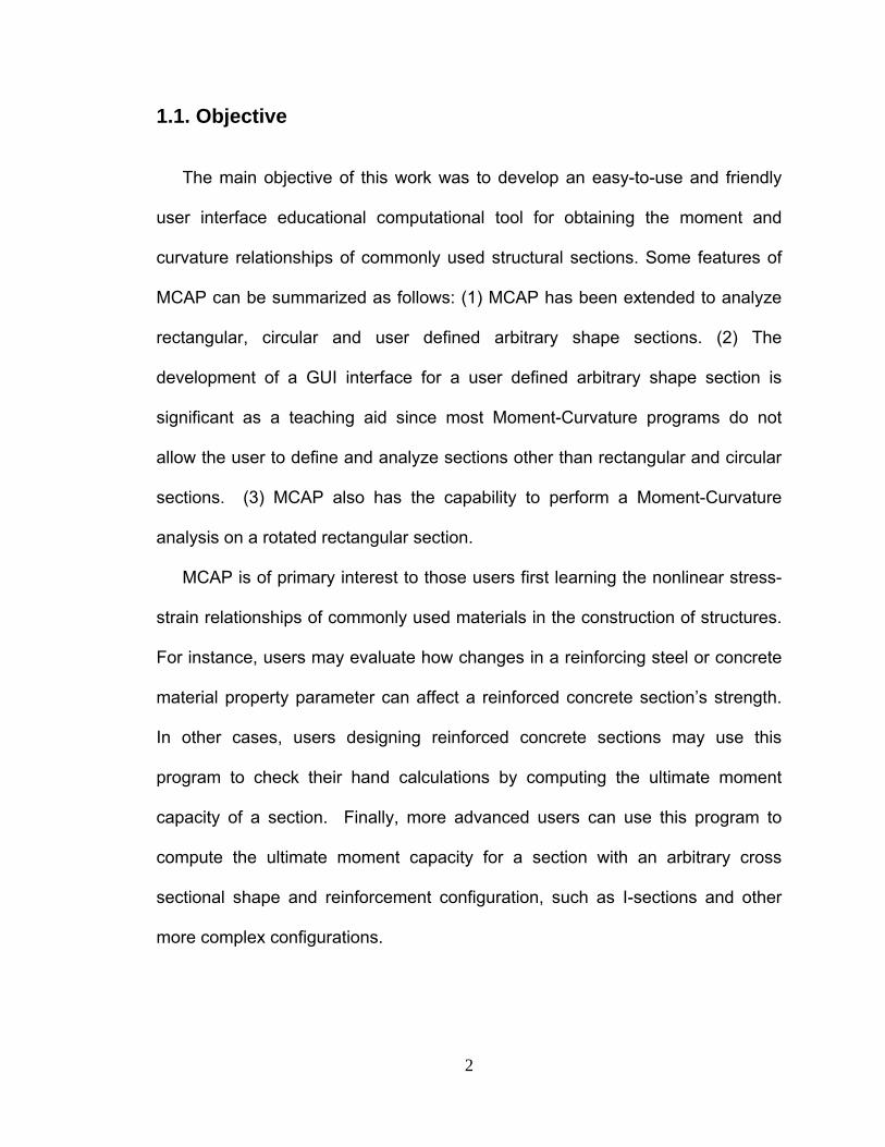
1.1. Objective

The main objective of this work was to develop an easy-to-use and friendly

user interface educational computational tool for obtaining the moment and

curvature relationships of commonly used structural sections. Some features of

MCAP can be summarized as follows: (1) MCAP has been extended to analyze

rectangular, circular and user defined arbitrary shape sections. (2) The

development of a GUI interface for a user defined arbitrary shape section is

significant as a teaching aid since most Moment-Curvature programs do not

allow the user to define and analyze sections other than rectangular and circular

sections. (3) MCAP also has the capability to perform a Moment-Curvature

analysis on a rotated rectangular section.

MCAP is of primary interest to those users first learning the nonlinear stress-

strain relationships of commonly used materials in the construction of structures.

For instance, users may evaluate how changes in a reinforcing steel or concrete

material property parameter can affect a reinforced concrete section’s strength.

In other cases, users designing reinforced concrete sections may use this

program to check their hand calculations by computing the ultimate moment

capacity of a section. Finally, more advanced users can use this program to

compute the ultimate moment capacity for a section with an arbitrary cross

sectional shape and reinforcement configuration, such as I-sections and other

more complex configurations.

3

1.2. Results

The results of a successful program will be an effective teaching aid which

combines the Graphical User Interface of MATLAB® and the power and

efficiency of OpenSees to create Moment-Curvature analyses.

The relationship between curvature and the strain in the extreme steel tension

layer is shown to be linear. This simple finding provides for faster convergence

in M-φ programs by being able to predict strain levels at the different steps in the

programs.

1.3. Organization

This thesis consists of 5 chapters. Chapter 1 provides an introduction and

main objectives of the thesis. Chapter 2 provides a succinct review of the

literature and software programs that are commonly used for conducting an M-φ

analysis as well as the interfaces used to create MCAP. A description of the

MCAP Modules and User’s Manual is provided in Chapter 3. Chapter 4

discusses the applications of MCAP and some findings concerning the

relationship between curvature and the tensile strain in the extreme reinforcing

layer. Chapter 5 includes conclusions about MCAP.

4

Chapter 2 - Literature Review: Moment-Curvature Analysis

MCAP is mainly an interface program that uses graphics building subroutines

from the standard MATLAB® library and subsequently creates the input files that

are necessary to run the OpenSees procedures and commands required to

perform M-φ analyses. In order to expedite the use and/or understanding of

MCAP, this section presents an overview of typical information necessary to

develop an M-φ analyses program. Salient points of an M-φ analysis program are

the: (1) geometry of the section and the respective modeling parameters

necessary to model the cross section of a member, (2) the nonlinear stress-strain

relationships to model the material properties used in the section, (3) the ultimate

or limiting strains for each of the materials, and (4) mathematical formulation of

the program. Understanding many of these items was an essential part in

creating the MCAP graphical user interface program.

Certainly, there are several other programs which can perform M-φ analysis

and each program has its merits and drawbacks. This section includes an

overview of programs current available in the literature for use in moment-

curvature analysis and concludes with an overview of MATLAB®, which served

as the GUI for MCAP.

2.1. Moment-Curvature Procedure

There exists an extensive body of information in the literature that details the

steps involved in performing a Moment-Curvature analysis for either using simple

5

hand calculations or for computer implementation. Figure 2-1a shows typical

section information required to establish an M-φ analysis.

Figure 2- 1: Typical Section, Strain Distribution and Actual Force Distribution

From its sectional geometry and for the given curvature, , Figure 2-1b

depicts the linear variation of strains along the section height by ensuring that

strains at a constant depth, dbi, are identical. According to the Euler-Bernoulli

theory of slender beams the linear variation of strains satisfies the principle that

‘plane sections’ before loading ‘remain plane' after loading. This infers that any

deformations within the section caused by shear are not accounted for in the

analysis. As such, the strains in the steel bars at any depth, , are obtained

based on the strain compatibility equation 2.1:

(2. 1)

Likewise, the strains in the concrete at any depth, , are obtained based on

the strain compatibility equation 2.2:

(2. 2)

c

Fy

P Mh

b

dsi

si

Fc

Fsi

(a) X-Section (b) Strain (c) Actual Force Distribution Distribution

cc

s

6

This linear variation of strains makes it possible to create the stress

distribution of Figure 2-1c, and subsequently the internal forces equilibrium

necessary to obtain the moment capacity of the section.

The first step in an M-φ analysis program is the division of the section in fibers

or segments, which is schematically shown in Figure 2-2. Each of these fibers or

segments are properly defined in terms of their center position to a reference

line, which in Figure 2-2 is the top of the section, area, and as importantly the

nonlinear stress-strain model.

Figure 2- 2: Discretization of a Concrete Section in Fibers

The next step involves assigning the curvature,  , and estimating the strains

in the top fibers, , which in conjunction with the fibers position, or , are

used to develop the strain compatibility equations.

To further enhance classroom instruction a supplementary moment-curvature

program was also implemented using MATLAB®. This supplementary program

was created to allow users unfamiliar with a moment curvature analysis to

understand the steps required to such an analysis. The code for this

h

b

dCi

dsi

7

supplementary program is in Appendix D. One of the innovative features in the

programming of this supplementary program is the implementation of a linear

relationship between the curvature and the strains in the extreme steel fibers,

which was used to reduce the iterations required to convergence, which is

discussed next. The rationale to establish the curvature increments involved in

MCAP are outlined later within this section.

Once the strain distribution is determined along the depth of the section, the

stresses in each of the fibers or segments is formulated from the respective

nonlinear stress-strain models.

The next step involves computing the internal forces in each of the fibers or

segments. In conjunction with the externally applied load, , the internal forces

in the concrete,  ∑ , and in the reinforcing steel,  ∑ , are used

in equation 2.3 to determine the equilibrium conditions of the section.

(2. 3)

If the equality in the equation above is satisfied the program proceeds to the

next step, otherwise the strains in the top fibers, , are estimated once again

and the procedure repeats itself until the equality is satisfied.

The next step involves computing the moment capacity, , for the assigned

curvature in terms of equation 2.4:

(2. 4)

8

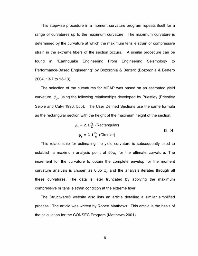
This stepwise procedure in a moment curvature program repeats itself for a

range of curvatures up to the maximum curvature. The maximum curvature is

determined by the curvature at which the maximum tensile strain or compressive

strain in the extreme fibers of the section occurs. A similar procedure can be

found in “Earthquake Engineering From Engineering Seismology to

Performance-Based Engineering” by Bozorgnia & Bertero (Bozorgnia & Bertero

2004, 13-7 to 13-13).

The selection of the curvatures for MCAP was based on an estimated yield

curvature, , using the following relationships developed by Priestley (Priestley

Seible and Calvi 1996, 555). The User Defined Sections use the same formula

as the rectangular section with the height of the maximum height of the section.

. (Rectangular)

. (Circular) (2. 5)

This relationship for estimating the yield curvature is subsequently used to

establish a maximum analysis point of 50φy for the ultimate curvature. The

increment for the curvature to obtain the complete envelop for the moment

curvature analysis is chosen as 0.05 φy and the analysis iterates through all

these curvatures. The data is later truncated by applying the maximum

compressive or tensile strain condition at the extreme fiber.

The Structware® website also lists an article detailing a similar simplified

process. The article was written by Robert Matthews. This article is the basis of

the calculation for the CONSEC Program (Matthews 2001).

9

An analysis routine performed by integration of basic equations can be found

in “Seismic Design Aids for Nonlinear Analysis of Reinforced Concrete

Structures” by Chandrasekaran et al. The procedure outlined includes

calculation of the moment for a given curvature by integration and evaluation of

constants of integration (Chandrasekaran et al. 2010, 45-88). This process lends

itself more readily to spreadsheets.

2.2. Nonlinear Material Models

It is critical in any Moment-Curvature analysis to apply an appropriate

nonlinear material model for either the concrete and/or the steel. Confined

concrete, unconfined concrete and steel models were used for MCAP. Much

work has been done in the past concerning models for confined concrete,

unconfined concrete and reinforcing steel, and the models used in MCAP are

discussed in the next sections.

2.2.1. Unconfined Concrete Models

Chang and Mander presented a review of concrete models and equations (Eq

2.6-2.13) for these models are shown below (Chang and Mander 1994, 3-1 to 3-

21).

10

2.2.1.1. Tsai’s Model (Chang and Mander 1994, 3-9)

Tsai’s Model, which is of the form of Equation 2.6 can describe confined and

unconfined concrete.

(2. 6)

Where, and (for all equations presented)

2.2.1.2. Popovic’s Model (Chang and Mander 1994, 3-5)

Tsai’s model is a generalization of Popovic’s Model shown in Equation 2.7:

(2. 7)

2.2.1.3. Young’s Models (Chang and Mander 1994, 3-3)

Young developed at three different relationships (Equations 2.8, 2.9, 2.10) for

the stress strain relationship of unconfined concrete:

(2. 8)

(2. 9)

11

(2. 10)

Where,

2.2.1.4. Mirza & Hsu Model (Chang and Mander 1994, 3-8)

Mirza and Hsu proposed a stress-strain relationship for unconfined concrete

detailed by equations 2.11 and 2.12:

. (2. 11)

Where x ,

. . . . . (2. 12)

Where x , .

2.2.1.5. Chang and Mander Model (Chang and Mander 1994, 3-12)

The Mander and Chang model used by OpenSees modeling command

“Concrete07” for confined and unconfined concrete is a variation of the Tsai

Model. It is essentially the Popovic Model with parameters (r and n) described by

Chang and Mander. Chang and Mander found this model to be the most

representative of high strength confined concrete (Chang & Mander 1994, 3-12).

The model is shown in Equation 2.13. MCAP uses this model.

12

(2. 13)

Where, ;  ; 

Figure 2-3 shows a graphical representation of Equations 2.6 through 2,13.

Equation 2.13 (the Chang and Mander Model) is the same as Equation 2.7 when

it is reduced down and the appropriate parameters are applied.

Figure 2- 3: Unconfined Concrete Model Comparison

2.2.2. Confined Concrete

2.2.2.1. Chang and Mander Model

The Chang and Mander Model can describe both confined concrete and

unconfined concrete. It is the model used to define concrete in the OpenSees

0 0.4 0.8 1.2 1.6 2

X=e/e'c

0

0.4

0.8

1.2

Y=

f/f'

c

Concrete ModelsEq 1: TsaiEq 2: PopovicEq 3: YoungEq 4: YoungEq 5: YoungEq 6 & 7: Mirza & Hsu

13

model used by MCAP. The Chang and Mander model is a well known concrete

model that has general agreement with experimental results for confined

concrete (Penelis and Kappos 1997, 194). To obtain stress values for confined

concrete, Equation 2.13 is simply multiplied by f’cc. The parameters for the Chang

and Mander Model are shown in Equations 2.14 & 2.15.

The strain at peak stress and peak stress are given by Mander, Priestley and

Park in Equations 2.14 and 2.15 respectively (Mander, Priestley and Park 1988).

  (2. 14)

  . ..

   (2. 15)

For Rectangular Sections:

  

  

∑

  

and

For Circular Sections:

  

  

14

  

  

The Mander Model also uses values to define the variable “r” in Equation

2.13. The values are found by using Equation 2.16:

(2. 16)

Where,

For rectangular sections, the following relationship in Equation 2.17 for

confinement index, K, was developed by Chang and Mander (Chang and Mander

1994, 3-32).

..

(2. 17)

Where,  

  ,  

. . . .

.

. . . . 

When the confining pressure in both directions is the same, a triaxial state of

stress is achieved and the confining pressure boils down to the following

relationship in equation 2.18 (Chang and Mander 1994, 3-32):

15

(2. 18)

2.2.2.2. Piecewise Models

Park, Priestley and Gill proposed a model that is a piecewise function

(Penelis and Kappos 1997, 183-184). Another commonly accepted piecewise

model is the Sheikh and Uzumeri model (Penelis and Kappos 1997, 183-184).

The models are detailed in Figure 2-4. Both of the models are empirically

determined and rely on a confinement index, K, to determine f’cc.

(A)

(B)

Figure 2- 4: Park, Priestley and Gill Concrete Model (A), Shiekh and Uzumeri Concrete Model (B)

2.2.3. Maximum Concrete Strain

One of the relationships used for evaluation of the M-φ curve is the ultimate

strain of unconfined concrete and confined concrete. Since the M-φ relationship

Strain

Str

ess

Confined Concrete CurvePark, Priestley and Gill Model

Strain

Str

ess

Confined Concrete CurveSheikh and Uzumeri Model

εcc

f’cc

0.2 f’cc

0.3 f’cc

εcc

f’cc

16

lends itself to dynamic analysis of RC structures, a limit from seismic engineering

literature were chosen.

For unconfined concrete was taken as 0.004 in/in. This value represents

the spalling strain of the concrete and is generally accepted in sections with

confined concrete cores and unconfined concrete cover (Penelis and Kappos

1997, 178). The equations for given by Priestley and Paulay are shown in

Equation 2.19 for circular and rectangular sections (Priestley and Paulay 1992,

103). The expression in Equation 2.19 is the expression used in MCAP.

. . /      (2. 19)

Where, for rectangular sections

2.2.4. Reinforcing Steel

There are several different representations of the reinforcing steel stress-

strain relationship. The overall shape of the Moment-Curvature relationship is as

much determined by the reinforcing steel as the concrete stress-strain model. It

is in fact the reinforcing steel with gives tensile capacity to the section and allows

for moment capacity above the cracking moment of the section. The yield

plateau of the steel and plastic region of reinforcing steel stress-strain behavior

defines the Moment-Curvature above the yield curvature. Therefore both the

elastic range and plastic range of the reinforcing steel stress-strain relationship

are of interest in selecting a steel model for use by the analysis program.

17

2.2.4.1. Kent and Park Model (Kent and Park, 1973, 98-103)

The model researched by Kent and Park and shown below in Equations 2.20-

2.23 (Kent and Park, 1973) uses the Ramberg-Osgood function and

experimentally determined parameters to develop a cyclical stress strain curve

for reinforcing steel. The equations for the stress-strain curve and

experimentally derived parameters are indicated below.

(2. 20)

. .

. (2. 21)

When n is odd:

. ..

(2. 22)

When n is even:

. ..

(2. 23)

2.2.4.2. Park Model (Park and Paulay 1975, 229)

The Park Model for the plastic region of steel for Monotonic loading of

reinforcing steel is given by equation 2.24 (Park and Paulay 1975, 229). This is

the model used by CONSEC and BENT for modeling of the reinforcing steel.

(2. 24)

18

Where, and

The elastic region of the relationship    ) and yield plateau    )

are given by equations 2.25 and 2.26 respectively:

(2. 25)

(2. 26)

2.2.4.3. Chang and Mander Model (Chang and Mander 1994, 2-1 to 2-2)

The Chang and Mander stress-strain relationship for the plastic region of

reinforcing steel is given in equation 2.27 (Chang and Mander 1994, 2-1 to 2-2).

The monotonic portion of the plastic region is shown. The elastic portion and

yield plateau portion are given by equations 2.25 and 2.26 respectively. The full

text of the report also gives rules for cyclic loading that have the curve match well

with the Kent and Park model for cyclic loading (Chang and Mander 1994, 2-1 to

2-58).

(2. 27)

Where,

A comparison of the Park monotonic reinforcing steel model, Kent and Park

monotonic reinforcing steel model and the Chang and Mander monotonic

19

reinforcing steel model are shown in Figure 2-5. All three models have a

significant difference in the representation of the plastic region of the stress-strain

curve.

Figure 2- 5: Reinforcing Steel Model Comparison

The reinforcing and concrete models provide the stress-strain basis for the

materials used in the determination of the moment and curvature values in the

moment-curvature plot. Different models will have an effect on the shape and

maximum values in the M-φ relationship. If more models become available for

use by OpenSees, different M-φ relationships can be developed.

0 0.02 0.04 0.06 0.08 0.1 0.12Strain (in/in)

0

10

20

30

40

50

60

70

80

90

100

Str

ess

(Ksi

)

Reinforcing Steel ModelsPark Steel ModelChang & Mander Steel ModelKent & Park Model

20

2.4. Available Moment-Curvature Computer Programs

The previous sections outlined the procedure used in developing the

monotonic moment-curvature envelope and the material models used in

developling the M-φ envelope. This section outlines a few M-φ programs for use

in obtaining the moment-curvature relationship of reinforced concrete sections.

This literature review is not meant to cover all programs used nowadays in

academia and/or industry but simply a brief outline of the main differences

between MCAP and other software programs.

2.4.1. OpenSees (Mazzoni et al., 2006)

OpenSees is a robust Finite Element Modeling program used for earthquake

simulation. It can perform Moment-Curvature analysis and is used for the

analysis portion of MCAP. It is free to anyone who registers. OpenSees does

not however currently have a Graphical User Interface specifically used for

Moment-Curvature analysis. This means that users need to manipulate scripts in

Notepad applications and run the script in a DOS prompt.

This process is overly complicated for first time users learning the important

relationships between material properties and section analysis. First time users

in an undergraduate setting may not be acclimated to programming in scripts.

Most beginning users in the undergraduate setting are used to a Graphical User

Interface to work with their software applications. Instead of learning the subject

matter of stress-strain and M-φ relationships, the typical undergraduate would be

21

first compelled to learn the programming involved in writing and running a script

in OpenSees. This would involve learning the syntax associated with OpenSees

and how to analyze the data resulting from the successful operation.

The complications for first time users using OpenSees prompted the

development of MCAP. The simplifications by MCAP to the process of entering

the material properties and performing the section analysis can increase

attention to the subject matter for undergraduates in engineering materials

classes.

OpenSees is the backbone of MCAP and performs the numerical analysis for

MCAP. OpenSees uses the Tcl (pronounced “tickle”) language. OpenSees

consists of 4 command groups that create and analyze the model. These four

groups are Modeling, Analysis, Recorder and Miscellaneous commands. Tcl

Scripts are created with the four command groups and then are run at the

OpenSees command prompt using the source command. The commands used

for creation of the moment-curvature analysis in MCAP are explained below.

2.4.1.1. Modeling Commands

OpenSees is a Finite Element modeling program. The modeling commands

allow the user to assemble a series of nodes and elements with all appropriate

material properties. Details for the modeling commands that are used in MCAP

are discussed next.

The “model BasicBuilder” command establishes the number of dimensions

and number of degrees of freedom for the model. The “node” command

22

establishes each node. For MCAP, 2 nodes are created for the section. A zero

length element is defined between the nodes to model the section using the

“element zerolengthSection” command. The “fix” command establishes the

restraints at each node. The material properties are defined by using the

“uniaxialMaterial” command. The section is divided up into fibers using the “fiber”

command with various methods to define the various fibers. In general, the more

fibers, the more precise the results are. The load pattern is defined using the

“pattern” command. A constant load pattern is used for MCAP.

2.4.1.2. Analysis Commands

Analysis parameters are established using “constraints” command (constraint

handler command), “integrator” command (load control, displacement control,

etc. for next time step), “numberer” command which is a DOF Numberer

command that maps the Degrees Of Freedom to the equations, “algorithm”

command which decides the solution techniques to be used, “system” command

which solves the equations within the solution algorithm, “test” command which

determines the convergence test and the “analysis” command which determines

which type of analysis is used (ie: Static). The analysis is completed using the

“analyze” command, which runs the analysis for the time step. One of the useful

features of MCAP is analysis parameters that can be switched if the program has

convergence issues. The subroutine for switching from one analysis parameter

to another was found in the examples manual on the OpenSees website

(Mazzoni and Mckenna 2006).

23

2.4.1.3. Recorder Commands

MCAP uses recorders to find the results of the analysis. A “node” recorder

records the nodal moment and curvature at the unrestrained node. An “element”

recorder records the stress and strain at a specific location within the section of

the zero-length element. The extreme fibers of compression or tension are

selected automatically to establish the ultimate limit state of the moment-

curvature analysis. Once the ultimate compression or tensile stress is reached

for the concrete or steel respectively, the data is later truncated by using

MATLAB®.

2.4.1.4. Miscellaneous Commands

Miscellaneous Commands are used to monitor the analysis during

computational steps. The analysis subroutine that will switch analysis

parameters in MCAP uses a “nodeDisp” command to monitor the current nodal

displacement of the unrestrained node. The “nodeDisp” Command also controls

the while loop in the previously mentioned subroutine.

2.4.2. SeismoStruct (Seismosoft 2011)

SeismoStruct is a Finite Element Modeling software program that allows the

user to perform Time History analysis and Push Over Analysis. It is available for

download from Seismosoft (Seismosoft 2011). It has a GUI and is a free

program for registered users. SeismoStruct allows users to choose between

several material models and element types. However, a more advanced

24

knowledge of Finite Elements is required to use the program. Also, one must

generate a complete, working Finite Element Model to generate a M-φ

relationship. The Program also restricts the user to several pre-defined shapes

and defining the reinforcement in a reinforced concrete member is more tedious

than with MCAP.

2.4.3. Response 2000 (Bentz 2011)

Response 2000 is cross-section and beam modeling software that models

reinforced and prestressed concrete beams and columns. It is available for

download for users who register at the Response 2000 website (Bentz 2011).

Response 2000 requires more time to master than MCAP and is meant for more

advanced non-linear analysis than MCAP. It is a useful tool and relatively easy

to learn, but has a few differences with MCAP. Response 2000 does not

internally compute the confinement of concrete materials but a user defined

model must be defined. Response 2000 also has several other types of pre-

defined sections.

2.4.4. BENT (Silva et al.)

BENT was created by Silva and Seible from UCSD and is a useful Moment-

Curvature analysis program for circular and rectangular sections. The program

does not have a Graphical User Interface and uses command prompts. MCAP

could serve as a replacement for BENT, as today’s users are accustomed to

computer software with GUI’s. A screenshot of BENT is shown in Figure 2-6.

25

BENT uses the same confinement models for concrete as MCAP but different

reinforcing steel models (Silva et al., 1999). The alternative reinforcing steel

models in BENT make it difficult to complete a direct comparison between BENT

and MCAP.

Figure 2- 6: Bent Application

2.4.5. CONSEC (Matthews 2009)

CONSEC was developed by Robert Matthews from Structware®. CONSEC

is free to download (Matthews 2009). It performs M-φ analysis and interaction

diagrams. The user interface is a Windows tab system. The sections are

developed with confined concrete and the Park model for reinforcing steel. It

performs moment curvature analysis on circular and rectangular sections.

2.5. MATLAB® Interface Used for MCAP

MATLAB® is a versatile programming language that has many predefined

functions. It is useful for numerical calculations, control of lab devices and

Graphical User Interfaces through predefined functions and “GUIDE”. MATLAB®

26

is based on the C++ language, but has been made easier to use through the

preprogrammed functions. Users also have the option of defining their own sub-

functions. The following sections describe the level of programming used for

MCAP.

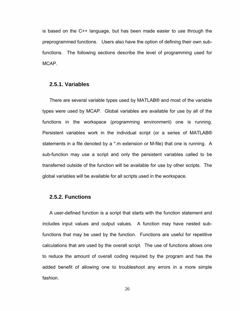
2.5.1. Variables

There are several variable types used by MATLAB® and most of the variable

types were used by MCAP. Global variables are available for use by all of the

functions in the workspace (programming environment) one is running.

Persistent variables work in the individual script (or a series of MATLAB®

statements in a file denoted by a *.m extension or M-file) that one is running. A

sub-function may use a script and only the persistent variables called to be

transferred outside of the function will be available for use by other scripts. The

global variables will be available for all scripts used in the workspace.

2.5.2. Functions

A user-defined function is a script that starts with the function statement and

includes input values and output values. A function may have nested sub-

functions that may be used by the function. Functions are useful for repetitive

calculations that are used by the overall script. The use of functions allows one

to reduce the amount of overall coding required by the program and has the

added benefit of allowing one to troubleshoot any errors in a more simple

fashion.

27

MATLAB® also includes functions that are available for use and are

preprogrammed into the code. Examples of these predefined functions are the

sine function with angle in degrees. The format for input and output of these

functions is found in the MATLAB® help section.

2.5.3. GUIDE and GUI Interfaces

MATLAB® uses the GUIDE command to create Graphic User Interfaces. The

GUIDE command opens a graphic user interface layout editor which allows one

to create the graphics for a GUI. The graphics are called figures. The scripts

used to run the figures are automatically created with the layout of the graphics.

For MCAP programming, the figure and script were created using the graphic

user interface layout editor. Once the script was created, different graphic user

interface options (for example a button) called subroutines created in other

MATLAB® scripts. This process was used to create each screen or figure in

MCAP. The buttons can call scripts containing other figures and graphics

screens.

The representations of shapes were plotted out into a set of axes embedded

into the GUI. Lists boxes and radio buttons were also used as necessary. The

drafting portion of the user defined shapes was created under a separate

subroutine which had its basis in an example code in the MATLAB® help menu.

28

2.5.4. Creating and Running OpenSees Files

OpenSees Tcl files are created by writing preformatted text and the variables

into a script Tcl file. The files are text files with a *.tcl extension. Two files are

actually simultaneously created in MCAP, one is “current.tcl” and the other is a

file named as the user has defined. The reason for this is the running of the

OpenSees File using MATLAB® commands. The command in MATLAB® that

allows the OpenSees file to execute is the bang command, which simply puts an

exclamation character (i.e.: “!”) in front of the executable file name and then an

ampersand and the command to be run. MATLAB® is not able to write the bang

command with a variable command name, so a static file to be rewritten and

rerun each time was created (the static file is “current.tcl”).

2.5.5. Data Analysis and Plotting

Some data analysis and plotting is used in MCAP. The results generated by

OpenSees are generally not in a readily usable form. MCAP uses MATLAB® to

process the data generated in the output files in OpenSees. Generally,

MATLAB® reads the text files generated by OpenSees and rewrites the data to a

text file formatted by MATLAB® that has headers and can be easily imported into

a spread sheet program. Finally, mathematic functions (ie: square roots, sums,

exponential, etc.) for calculating the various input for the materials models used

in the OpenSees Tcl scripts are also used.

29

MCAP also plots the data into the GUI’s created in GUIDE using plot

functions in MATLAB®. Various plot functions such as the plot and line function

are used to create the graphics depicting the sections in MCAP.

30

Chapter 3 - MCAP User’s Manual and Development Information

The following section outlines a User’s manual and the development

information for MCAP. The interface is intuitive, but some simple installation

instructions are followed by a guide on the operation of MCAP. It should be

noted that MCAP requires that OpenSees first be installed on your computer.

OpenSees is available for download for those who register from the OpenSees

Website. MCAP is initiated in MATLAB® through typing “Main” at the command

prompt.

3.1. Installation Instructions

Step 1: Copy MCAP Version 1.5 Folder to a convenient directory on

your computer.

Step 2: Install OpenSees on your computer (see

http://opensees.berkeley.edu/ for instructions).

Step 3: Make sure OpenSees.exe and LibUnits.tcl are in the MCAP

Folder.

3.2. Running MCAP

Step 1: Open MATLAB®. Set Screen Resolution to 1200x800.

Step 2: Browse to the MCAP Version 1.5 Directory.

Step 3: Type “Main” at the command prompt.

31

Figure 3- 1: Command to Run MCAP Once Installed

Step 4: The MCAP main menu appears.

Figure 3- 2: MCAP Title Screen

32

Step 5: Choose section type (ie: Rectangular, Circular or User

Defined)

Figure 3- 3: Choose Section Analysis Type

3.3. Section Analysis Title Screens

The section analysis title screens (see Figure 3-4) are all the same with the

exception of the graphic showing the direction of the moment for the section.

The analysis process for running an analysis in MCAP is the same for all three

modules. First we define the section. This is followed by the material properties

of the section elements (ie: steel and concrete). Then the *.TCL file for

OpenSees analysis is created. Next the section is analyzed. Then the Moment-

Curvature plot is displayed. Finally, we can exit the module if we want using

“Back to Title Screen”.

33

Figure 3- 4: Module Title Screen

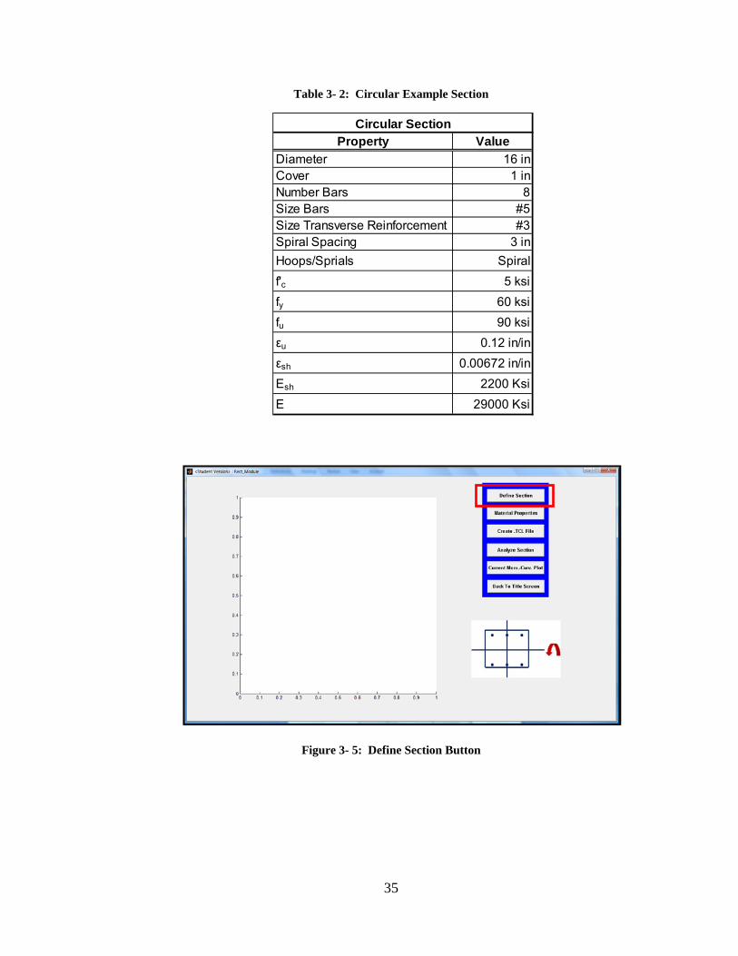
3.4. Defining Sections

Once the “Define Section” button (see Figure 3-5) is clicked the section

definition screens are shown. Figures 3-6, 3-7 & 3-8 show the section definition

screens for each module. Test sections will be used for this chapter. The

desired properties are shown in Tables 3-1 & 3-2 for rectangular and circular

sections respectively. The User Defined section will be 24” high, 16” wide, a 6”

top and bottom flange, a web 6” wide and a 2” taper from the flange to

connection with the web. There will be 4 - #6 Bars top and bottom with a #4

transverse reinforcement layer. The cover will be 1”. The confining pressure will

be 0.15 ksi. For all sections the axial load will be 10 kips in compression.

34

Table 3- 1: Rectangular Example Section

Property Value

Height 16 inWidth 12 inCover 1 inNumber of Top & Bottom Bars 4Number of Side Bars 0Size Top & Bottom Bars #4

Size Transverse Reinforcement #3

Spacing Transverse Reinforcement 4 in

Number of Legs in X Direction 2

Number of Legs in Y Direction 2

Rotation Angle 0 Degrees

f'c 5 ksi

fy 60 ksi

fu 90 ksi

εu 0.12 in/in

εsh 0.00672 in/in

Esh 2200 Ksi

E 29000 Ksi

Rectangular Section

35

Table 3- 2: Circular Example Section

Figure 3- 5: Define Section Button

Property Value

Diameter 16 inCover 1 inNumber Bars 8Size Bars #5Size Transverse Reinforcement #3Spiral Spacing 3 in

Hoops/Sprials Spiral

f'c 5 ksi

fy 60 ksi

fu 90 ksi

εu 0.12 in/in

εsh 0.00672 in/in

Esh 2200 Ksi

E 29000 Ksi

Circular Section

36

Figure 3- 6: Rectangular Section Definition

Figure 3- 7: Circulat Section Definition

37

Figure 3- 8: User Defined Section Definition

For the rectangular and circular sections, define the section dimensions

shown in the boxes. The rectangular module allows the user to rotate the section

if a rotated analysis is desired. Click on “Draw Section” as shown in Figures 3-10

& 3-11. An image of the section will appear. Press return/exit to go back to the

module title screen and move on.

The rotation angle in the rectangular section lets the user rotate the section

counter clockwise from zero degrees to 90 degrees. This gives the user a larger

range of configurations to choose from and this option is not available through

most Moment-Curvature programs. The section is rotated by using a

transformation matrix to define each patch area. The test section was rotated

zero degrees, 45 degrees and 90 degrees CCW. The results of the rotation of

the section are shown in Figure3-9. As expected, the section capacity is

diminished with increased rotation through 90 degrees.

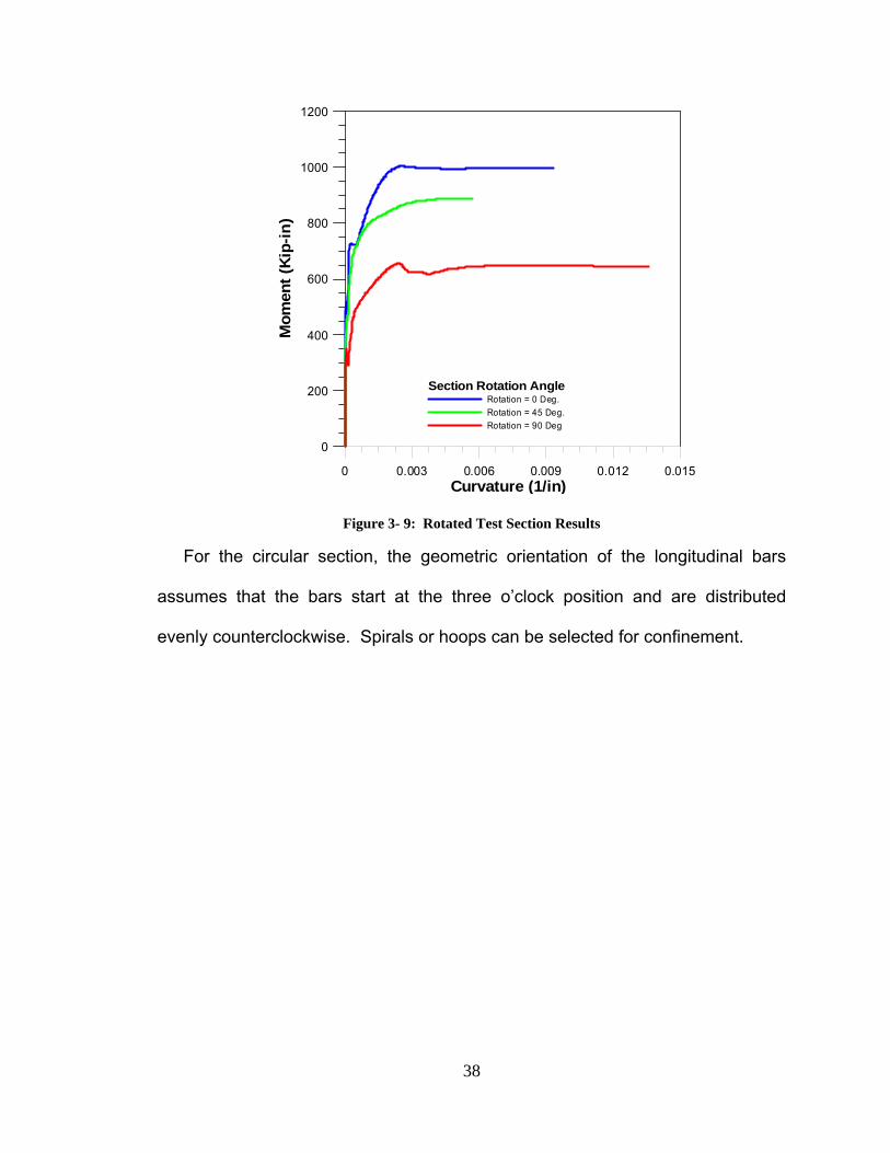
38

Figure 3- 9: Rotated Test Section Results

For the circular section, the geometric orientation of the longitudinal bars

assumes that the bars start at the three o’clock position and are distributed

evenly counterclockwise. Spirals or hoops can be selected for confinement.

0 0.003 0.006 0.009 0.012 0.015Curvature (1/in)

0

200

400

600

800

1000

1200

Mo

men

t (K

ip-i

n)

Section Rotation AngleRotation = 0 Deg.

Rotation = 45 Deg.

Rotation = 90 Deg

39

Figure 3- 10: Draw Rectangular Section

Figure 3- 11: Draw Circular Section

The section definition for the user defined section is more complicated. The

section must be drawn. The User Defined module allows the user to draw the

section down to the sixteenth of an inch. Subroutines (windows_motion_test.m

and draw_lines.m) in the MATLAB® examples manual section were modified

40

significantly to create the drawing application in MCAP (The MathWorks 2007).

The user defined section definition title screen has several settings for grid, snap

and drawing canvas size. Set these boxes to what you will need for your section.

For the example, the settings will be a snap of ½”, a grid of 1” and a drawing

canvas size of 24” (which is 24” x 24”). Next press the “Draft Section” Button. A

drawing grid or canvas will pop up (see Figure3-12). Left click on all corners of

your section. Right Click on the last point to close the section and window. It is

important that all subsequent points for the transverse steel and core definition

be defined in the same order from start point location to end point location.

Figure 3- 12: User Defined Section Drawing Canvas

41

Figure 3- 13: User Defined Section

Continue through the user defined section drawing buttons to define the

transverse reinforcement (with the proper cover requirements), longitudinal

reinforcement and to define the core area. Keep in mind that you start with a left

click and end with a right click. You can define the longitudinal steel all at one

time. Always start and follow the same order for the section extents, transverse

reinforcement and core area definition. Try to define the core area as close to

the Transverse Reinforcement center line as possible.

42

Figure 3- 14: Define the Transverse Reinforcement

Figure 3- 15: Define Longitudinal Reinforcement

43

Figure 3- 16: Define Core Area

Figure 3- 17: Completed User Defined Section

After the core area is defined, click on draw section. At this point, the section

definition can also be saved (see Figure 3-17). Click on Exit to return to the user

defined module title screen.

44

3.5. Material Properties

The material properties screen is essentially the same for all three modules.

The OpenSees models used for MCAP are “concrete07” for concrete and

“reinforcingsteel” for the reinforcement. The user defined module requires that

the confining pressure, fl’ be defined for the concrete (see Figure3-19). The steel

properties menu allows the user to load a lab test data and graphically match the

lab data with the steel model used. The lab data file should be a tab delimited

text file with the strain values in the first column and stress values in the second

column. To load the lab tested values click on the “Load” button, select the file

and then click on plot steel model (see Figure3-20). Also, plot the concrete

model after the steel model has been defined. As the steel properties have an

effect on the confinement in the Chang-Mander Model.

For the circular section, Equations 2.14, 2.15 and 2.16 are used to detail the

confined concrete. The Chang and Mander model is used to detail the

reinforcing steel. The OpenSees material models are again “concrete07” and

“reinforcingsteel”

The confinement of the concrete for rectangular sections is controlled by the

number of legs of reinforcing steel in each of the x and y directions of the section.

The confinement in each direction may be different, so the relationship described

by Chang and Mander for determining the peak confined concrete stress was

used. This relationship is given by equation 2.17 (Chang and Mander 1994, 3-

32).

45

The confining pressure for the user defined module is determined by the user

and the peak confined stress is determined using the Chang and Mander model

in Equation 2.15. Estimating the user defined confining pressures will result in a

learning process for the user.

Figure 3- 18: Material Proplerties Screen - Rectangular and Circular Sections

Figure 3- 19: Confining Pressure fur User Defined Material Properties

46

Figure 3- 20: Defining Material Models

3.6. Create *.Tcl File

After definition of the section and definition of the material properties, the *.Tcl

file needs to be created. This is the file that OpenSees uses to perform the

analysis. Sample files created by MCAP are shown in Appendices A, B & C for

the rectangular, circular and user defined test sections respectively. Figure 3-21

shows the screen for the rectangular and circular modules. Type in the file name

without extension and enter the axial load in kips. The axial force is assumed to

be in compression (ie: a column). Therefore, a positive value of 10 kips indicates

10 kips in compression. Click on “Create .Tcl File” and “Return” to get back to the

module title screen.

47

Figure 3- 21: Create *.Tcl Screen - Rectangular and Circular Modules

The user defined module has an extra step. The patches required for the

section must be defined. Enter the number of patches in the X and Y direction

and then click on “create patches” (see Figure3-22). After the patches are

displayed, enter the file name, axial load and then click on “Create .Tcl File”.

Click on “Return” to return to the module title screen.

Figure 3- 22: Creating the *.Tcl File for User Defined Sections

48

The main challenge in defining a model in OpenSees for the User Defined

Module is that the shape of the section was not known. In order to address this

unknown, a method for dividing the section into patches for implementation into

OpenSees was created. Moreover, the region of the section bounding the

confined concrete and the cover concrete was treated separately. To do this

task, the main cross section was divided up into points on a grid. If the points

were within the confines of the sub-section, they were included in the sub-section

and material properties and areas were assigned to the coordinates. This was

not a trivial task. It required significant and challenging programming in

MATLAB®. After a few cycles of programming, a technique was developed that

can be implemented d for most any common RC sections. The area, say a

rectangle is confined by 4 lines (ie: the transverse reinforcement). As part of the

input of the section, the confined area is described by 4 lines interior to the

transverse reinforcement lines describing the side of the confined concrete

section. Each point that is on the same side of the section boundary line as the

line describing the confined area has a value added to its count. By doing this for

each line in the rectangle, the points on the interior have a count value of 4 and

the points to the exterior have a count value less than 2. Through trial and error

and some manipulation of the values added to each point for various cases, it

was found that the interior point count greater than 2.5 to 3.33 were indeed

interior points and the points less than this value were exterior points. A sample

graphic of this technique is shown by the interior (confined) rectangle in Figure 3-

23.

49

Figure 3- 23: Method for Determining User Defined Patches

The cover concrete patches were easier to determine. If the points were

between the exterior line of the section and the transverse reinforcement line,

they were kept and material properties were assigned. Careful attention had to

be made to the statements describing the points in between the lines. But

through a series of 4 switch cases, this was accomplished.

It should be noted in the analysis of the sections that OpenSees does not

determine the end point of the M-φ analysis. The analysis is carried to 50φy and

then the analysis is truncated by either the extreme compressive strain or

extreme tensile strain reaching its ultimate strain. This process occurs for each

module of MCAP.

4 4 4

4 4 4

4 4 4

1 1 1

1 1 1

1

1

1

1

1

1

00

00

50

3.7. Analyzing the Section

The section analysis is done using the “Analyze Section” Button. Once the

section, material properties and *.Tcl file are defined, Click on “Analyze Section”

(see Figure3-24). When the analysis is complete a pop-up box will appear

showing that the analysis is complete. The analysis is completed using the

“bang” command in MATLAB® to run the “current.tcl” file created by MATLAB®

in OpenSees.

Figure 3- 24: Analyze Section

3.8. Moment-Curvature Plot (and Data)

The Moment Curvature Plot is created after the analysis is complete. Simply

click on “Current Mom.-Curv. Plot” (see Figure3-25) after the analysis is complete

to display the plot. Upon plotting of the results, a file is created which has the M-

φ data from the analysis as well as the neutral axis position, steel stress and

concrete stress. This information can be plotted by the user in a spreadsheet

51

program for using the results outside of MCAP. This data file is in a folder where

MCAP is located with the same name as the file name previously entered in

section 3.6. A screen shot of the sample plot is shown in Figure3-25. Click on

the Back to Title Screen button to switch between modules.

Figure 3- 25: Moment-Curvature Plot

3.9. Results for Test Sections

The results for the test sections previously described are shown in Figures 3-

26 to 3-28.

52

Figure 3- 26: Rectangular Test Section M-C Plot

Figure 3- 27: Circular Test Section M-C Plot

53

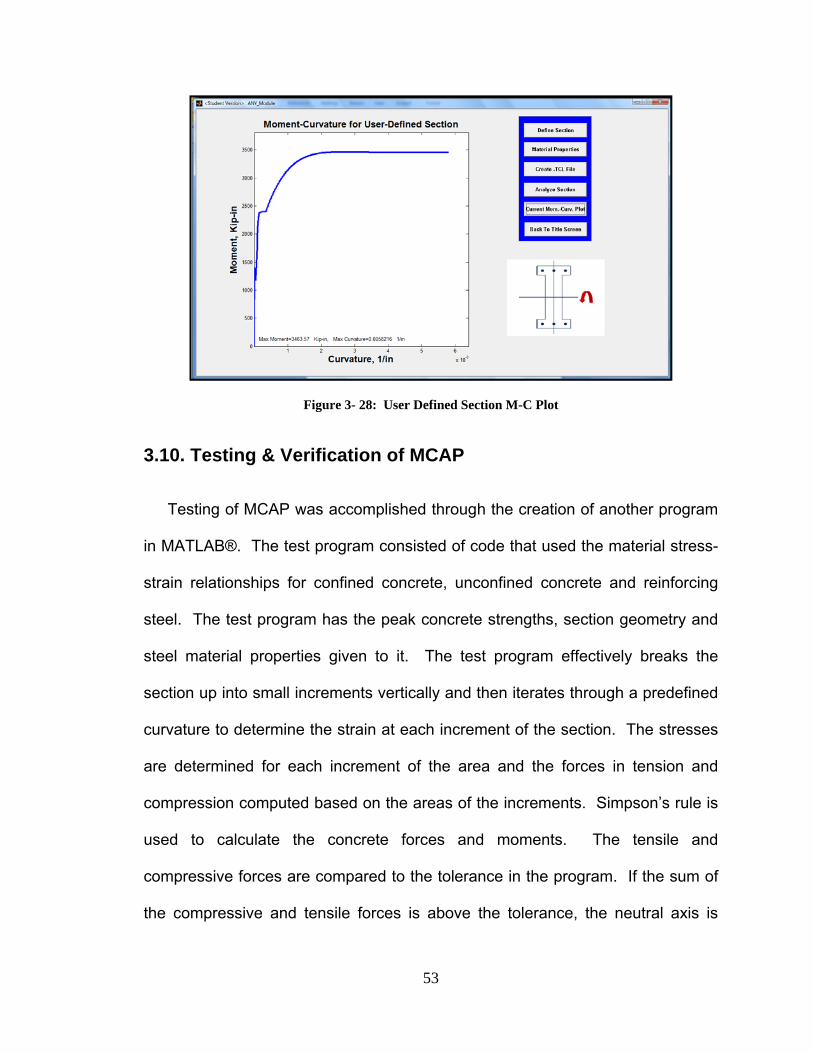
Figure 3- 28: User Defined Section M-C Plot

3.10. Testing & Verification of MCAP

Testing of MCAP was accomplished through the creation of another program

in MATLAB®. The test program consisted of code that used the material stress-

strain relationships for confined concrete, unconfined concrete and reinforcing

steel. The test program has the peak concrete strengths, section geometry and

steel material properties given to it. The test program effectively breaks the

section up into small increments vertically and then iterates through a predefined

curvature to determine the strain at each increment of the section. The stresses

are determined for each increment of the area and the forces in tension and

compression computed based on the areas of the increments. Simpson’s rule is

used to calculate the concrete forces and moments. The tensile and

compressive forces are compared to the tolerance in the program. If the sum of

the compressive and tensile forces is above the tolerance, the neutral axis is

54

moved and the process starts again for the given curvature. Once the tensile

and compressive forces are in balance the moment about the plastic center is

taken and the moment and curvature are recorded. The same technique was

used to calculate the moment-curvature relationship for rectangular and circular

sections. As shown in Figures 3-29 and 3-30, the results for both circular and

rectangular sections show the OpenSees analysis and test program analysis to

be consistent with each other. The tables 3-1 & 3-2 show the section properties

of the test program comparison.

To test the user defined sections, a rectangle was created through the user

defined module with the confining pressure matching the confining pressure for a

rectangular section of the same configuration. The analysis showed that the

rectangular section analysis, user-defined section analysis and test program

analysis all matched closely which seems to indicate that each analysis is

accurate as the same results are obtained using different processes.

MCAP was also compared versus Response 2000. The plots in Figures 3-29

to 3-31 show that the overall capacity of the section was similar for all three

sections reviewed. Table 3-3 shows the properties for the “I” section. There

were some differences on the non-linear portions of the curve and the extreme

curvature values. The differences in the plots were caused by different

reinforcing steel material models and the lack of a confined concrete model in

Response 2000. The plastic region of the steel models was very different as

shown in Figure 2-5. The continued value of stress with increased strains with a

confined concrete model would allow the moment values for the Response 2000

55

curves to be higher at larger curvature values if a confined concrete model was

used. With these two adjustments the plots would be very similar.

Table 3- 3: “I” Section Properties for Verification

Property Value

Height 24Width 24Cover 1 inWeb Thickness 12 inFlange Thickness (Top & Bottom) 8 inNumber of Top & Bottom Bars 6Number of Side Bars 0Size Top & Bottom Bars #6Size Transverse Reinforcement #3Spacing Transverse Reinforcement 4 inNumber of Legs in X Direction 2Number of Legs in Y Direction 2Rotation Angle 0 Degrees

f'c 5 ksi

fy 60 ksi

fu 90 ksi

εu 0.12 in/in

εsh 0.00672 in/in

Esh 2200 Ksi

E 29000 Ksi

I Section

56

Figure 3- 29: Comparison between Rectangular Section Programs

Figure 3- 30: Comparison between Circular Section Programs

0 0.005 0.01Curvature (1/in)

0

100

200

300

400

500

600

700

800

900

1000

1100

Mo

men

t (K

ip-i

n) Analysis Technique

MCAP User-Defined Rectangle

Practice Program

MCAP Rectangular Section

Response 2000

0 0.003 0.006 0.009Curvature (1/in)

0

200

400

600

800

1000

1200

1400

Mo

men

t (K

ip-i

n)

Analysis TechniqueMCAP Circular Module

Practice Program

Response 2000

57

Figure 3- 31: Comparison between "I" Section Programs

0 0.003 0.006Curvature (1/in)

0

800

1600

2400

3200

4000

4800

5600

Mo

men

t (K

ip-i

n)

Analysis TechniqueMCAP I Section

Response 2000 I Section

58

Chapter 4 - MCAP Applications

The primary purpose of MCAP is to serve mainly as a teaching aid. There

are many teaching aid applications and a few are listed in the following sections.

Material properties, introductions to the design of structures, testing of theoretical

predictions and many other concepts can be explained with the help of MCAP.

Most of these ideas consist of determining moment capacity of a section. Both

elastic and inelastic behavior of a section is determined by MCAP.

4.1. MCAP as a Teaching Aid

The underlying OpenSees Code for MCAP was used in the GWU Fall 2009

CE Materials Laboratory class to predict the failure moment for a simply

supported RC beam under load. Undergraduates were asked to predict the load

and ultimate moment at which the beam would fail. After the test, when the load

and moment were known, undergraduates were then able to alter material model

assumptions to see how the material properties affected the strength of the

beam. This exercise also provided a glimpse into design of beams to see how

spacing and size of reinforcement as well as material properties affect the

strength of a RC Section.

Material testing and strength is critical to structural design. MCAP users will

be able to learn how reinforcing confinement alters the strength of a concrete

section. A module could be added to allow users to create confined concrete

specimens, test them and compare the results to the predicted model.

59

Users can also currently test reinforcing steel in the lab and compare the

actual stress-strain relationship to the theoretical relationship given by the Chang

and Mander Model by reading the data in MCAP. The theoretical model can be

altered to match the actual test results and the material properties of the tested

reinforcing steel can be graphically determined. Once the steel is tested in the

lab, it can be placed in the model for a beam section analysis. Users can then

find and predict the ultimate moment of a simply supported beam. If the beam is

then created and tested in the lab, users can test their predictions with actual

members in the lab. By performing this process, users can be taught what

aspects of the material properties lead to beam failure, be it the tensile strength

of the steel or compressive strength of the concrete, etc. users can also predict

and observe the failure mode.

4.2. MCAP as a basis to find Force-Deformation Relationship

If one knows the Moment-Curvature relationship of a section and also knows

the structural configuration (ie: cantilever, simply supported beam, etc.) of a

member with the section, one can determine the force-deformation relationship of

the member using the Moment-Curvature Relationship. There are several

methods of doing this including the Euler Method and Runge-Kutta Method. For

either case, MCAP can provide the Moment-Curvature relationship that can then

be used to determine the force-deformation relationship.

60

4.3. MCAP as an analysis Tool

MCAP determines the complete moment-curvature relationship for a RC

section. The M-φ relationship generated by MCAP can be used to determine

yield moment and yield curvature (at first yield of the reinforcing steel). For a

given curvature ductility, the plastic moment value can determined from the

relationship generated by MCAP. The plastic moment can then be used to find

the location of the plastic hinge and the maximum loading for a member before it

becomes unstable. The yield curvature would also allow one to determine the

plastic hinge length for a member.

4.4. Relationship Between Reinforcing Strain and Curvature

Through comparing results in MCAP, it was found that there is a relationship

between the curvature of a section and the steel strain in the extreme tensile

reinforcing layer. The relationship is independent of the number of bars in the

extreme layer and independent of the shape of the section.

The relationship was found by analyzing 18 different sections with different

axial loads, geometry and material properties. Table 4-1 shows the different test

scenarios examined. The results of the analysis are shown in Figures 4-1 to 4-5.

For various sections, compressive axial force, no axial force and tensile axial

forces were examined. In each case the relationship of curvature vs. steel strain

was linear or very close to linear.

61

Table 4- 1: Strain vs. Curvature Test Sections

This relationship is useful for programmers of a Moment-Curvature software

program. Most programs iterate through many neutral axis positions to

determine the neutral axis position of the section where the compressive forces

and tensile forces are in balance. If the neutral axis is nearly known, the number

of iterations of the neutral axis position is greatly reduced, which results in a

program that is accurate and fast.

By performing a first iteration and finding the neutral axis position and the

steel strain at that position as well as knowing the two curvatures (current and

next iteration), one can predict the position of the neutral axis of the next iteration

closely. By using a linear relationship between the curvature and steel strain,

computational times are greatly reduced. This idea was used in the test program

for MCAP and was highly effective in reducing the computational time. In fact,

precision of the test program was increased because of the savings in the

iterations required to determine the neutral axis.

Test # Section Size ReinforcementSpacing

Trans. Reinf.Axial Load

(Kips)1 Rect. 16"x12" 4-#4 T&B - #3 Trans, 2x2 legs 4" -52 Rect. 16"x12" 4-#4 T&B - #3 Trans, 2x2 legs 4" 03 Rect. 16"x12" 4-#4 T&B - #3 Trans, 2x2 legs 4" 54 Rect. 24"x24" 6-#6 T&B, 6-#6 SB, #4 Tans, 3x4 legs 6" -255 Rect. 24"x24" 6-#6 T&B, 6-#6 SB, #4 Tans, 3x4 legs 6" 06 Rect. 24"x24" 6-#6 T&B, 6-#6 SB, #4 Tans, 3x4 legs 6" 257 Rect. 30"x36" 8-#8 T&B, 10-#8 SB, #5 Trans, 4x5 legs 8" -508 Rect. 30"x36" 8-#8 T&B, 10-#8 SB, #5 Trans, 4x5 legs 8" 09 Rect. 30"x36" 8-#8 T&B, 10-#8 SB, #5 Trans, 4x5 legs 8" 5010 Circ. 16" Dia. 16-#4 Long, #3 Sprials 3" -1011 Circ. 16" Dia. 16-#4 Long, #3 Sprials 3" 012 Circ. 16" Dia. 16-#4 Long, #3 Sprials 3" 1013 Circ. 24" Dia. 12-#8, #4 Hoops 2" -2514 Circ. 24" Dia. 12-#8, #4 Hoops 2" 015 Circ. 24" Dia. 12-#8, #4 Hoops 2" 2516 W 16"x15" 5-#8 Top, 4-#8 Bottom, #4 Trans 4" -517 W 16"x15" 5-#8 Top, 4-#8 Bottom, #4 Trans 4" 018 w 16"x15" 5-#8 Top, 4-#8 Bottom, #4 Trans 4" 5

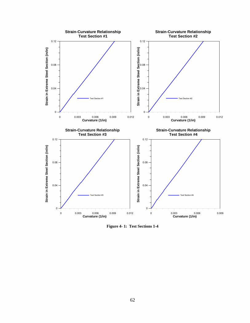
62

Figure 4- 1: Test Sections 1-4

0 0.003 0.006 0.009 0.012Curvature (1/in)

0

0.04

0.08

0.12

Str

ain

in E

xtre

me

Ste

el S

ecti

on

(in

/in)

Test Section #1

Strain-Curvature RelationshipTest Section #1

0 0.003 0.006 0.009 0.012Curvature (1/in)

0

0.04

0.08

0.12

Str

ain

in

Ext

rem

e S

teel

Sec

tio

n (

in/i

n)

Test Section #2

Strain-Curvature RelationshipTest Section #2

0 0.003 0.006 0.009 0.012Curvature (1/in)

0

0.04

0.08

0.12

Str

ain

in

Ext

rem

e S

teel

Sec

tio

n (

in/i

n)

Test Section #3

Strain-Curvature RelationshipTest Section #3

0 0.003 0.006 0.009Curvature (1/in)

0

0.04

0.08

0.12S

trai

n i

n E

xtre

me

Ste

el S

ecti

on

(in

/in

)

Test Section #4

Strain-Curvature RelationshipTest Section #4

63

Figure 4- 2: Test Sections 5-8

0 0.003 0.006 0.009Curvature (1/in)

0

0.04

0.08

0.12

Str

ain

in

Ext

rem

e S

teel

Sec

tio

n (

in/i

n)

Test Section #5

Strain-Curvature RelationshipTest Section #5

0 0.003 0.006 0.009Curvature (1/in)

0

0.04

0.08

0.12

Str

ain

in

Ext

rem

e S

teel

Sec

tio

n (

in/i

n)

Test Section #6

Strain-Curvature RelationshipTest Section #6

0 0.003 0.006Curvature (1/in)

0

0.04

0.08

0.12

Str

ain

in

Ext

rem

e S

teel

Sec

tio

n (

in/i

n)

Test Section #7

Strain-Curvature RelationshipTest Section #7

0 0.003 0.006Curvature (1/in)

0

0.04

0.08

0.12

Str

ain

in

Ext

rem

e S

teel

Sec

tio

n (

in/i

n)

Test Section #8

Strain-Curvature RelationshipTest Section #8

64

Figure 4- 3: Test Sections 9-12

0 0.003 0.006Curvature (1/in)

0

0.04

0.08

0.12

Str

ain

in

Ext

rem

e S

teel

Sec

tio

n (

in/i

n)

Test Section #9

Strain-Curvature RelationshipTest Section #9

0 0.003 0.006 0.009Curvature (1/in)

0

0.01

0.02

0.03

0.04

Str

ain

in

Ext

rem

e S

teel

Sec

tio

n (

in/i

n)

Test Section #10

Strain-Curvature RelationshipTest Section #10

0 0.003 0.006 0.009Curvature (1/in)

0

0.01

0.02

0.03

0.04

Str

ain

in

Ext

rem

e S

teel

Sec

tio

n (

in/i

n)

Test Section #11

Strain-Curvature RelationshipTest Section #11

0 0.003 0.006 0.009Curvature (1/in)

0

0.01

0.02

0.03

0.04

Str

ain

in

Ext

rem

e S

teel

Sec

tio

n (

in/i

n)

Test Section #12

Strain-Curvature RelationshipTest Section #12

65

Figure 4- 4: Test Sections 13-16

0 0.003 0.006 0.009Curvature (1/in)

0

0.01

0.02

0.03

0.04

0.05

Str

ain

in

Ext

rem

e S

teel

Sec

tio

n (

in/i

n)

Test Section #13

Strain-Curvature RelationshipTest Section #13

0 0.003 0.006 0.009Curvature (1/in)

0

0.01

0.02

0.03

0.04

Str

ain

in

Ext

rem

e S

teel

Sec

tio

n (

in/i

n)

Test Section #14

Strain-Curvature RelationshipTest Section #14

0 0.003 0.006 0.009Curvature (1/in)

0

0.01

0.02

0.03

0.04

Str

ain

in

Ext

rem

e S

teel

Sec

tio

n (

in/i

n)

Test Section #15

Strain-Curvature RelationshipTest Section #15

0 0.003 0.006 0.009Curvature (1/in)

0

0.04

0.08

0.12

Str

ain

in

Ext

rem

e S

teel

Sec

tio

n (

in/i

n)

Test Section #16

Strain-Curvature RelationshipTest Section #16

66

Figure 4- 5: Test Sections 17-18

4.5. Using the Reinforcing Strain – Curvature Relationship

As a way to verify how the reinforcing strain and curvature relationship might

be used another M-φ program was created in MATLAB® as a learning exercise.

The sample code for the rectangular section is shown in Appendix D. The

program consisted of code that used the same material stress-strain

relationships for confined concrete, unconfined concrete and reinforcing steel as

MCAP. The program has the peak concrete strengths, section geometry and

steel material properties given to it. Following the procedures outlined in Section

2, the program effectively breaks the section up into small increments (see

Figure 2-2) vertically and then iterates through a predefined curvature to

0 0.003 0.006 0.009Curvature (1/in)

0

0.04

0.08

0.12

Str

ain

in

Ext

rem

e S

teel

Sec

tio

n (

in/i

n)

Test Section #17

Strain-Curvature RelationshipTest Section #17

0 0.003 0.006 0.009Curvature (1/in)

0

0.04

0.08

0.12

Str

ain

in

Ext

rem

e S

teel

Sec

tio

n (

in/i

n)

Test Section #18

Strain-Curvature RelationshipTest Section #18

67

determine the strain at each increment of the section. The initial placement of

the neutral axis is determined by using the linear relationship between the tensile

strain in the extreme reinforcing layer and the curvature from the previous

iteration. The neutral axis is then fine tuned by moving it with an algorithm that

assumes a linear change in neutral axis position based on the amount of change

in tensile and compressive forces in the last iteration. The stresses are

determined for each increment of the area and the forces in tension and

compression computed based on the areas of the increments. Simpson’s rule is

used to calculate the concrete forces and moments. The tensile and

compressive forces are compared to the tolerance in the program. If the sum of

the compressive and tensile forces is above the tolerance, the neutral axis is

moved and the process starts again for the given curvature. Once the tensile

and compressive forces are in balance the moment about the plastic center is

taken and the moment and curvature are recorded. The same technique was

used to calculate the moment-curvature relationship for rectangular and circular

sections. As shown in Figures 4-6 and 4-7, the results for both circular and

rectangular sections show the OpenSees analysis and “practice” program

analysis to be consistent with each other. Tables 3-1 & 3-2 show the section

properties of the practice program comparison.

The process of finding the neutral axis position using the relationship

between tensile strain in the extreme layer and curvature assures the smallest

amount of iterations to find the right neutral axis position. In writing this program,

68

the time for the analysis was significantly reduced by incorporating a good initial

estimate for the neutral axis position.

Figure 4- 6: Rectangular Section Comparison

0 0.005 0.01Curvature (1/in)

0

100

200

300

400

500

600

700

800

900

1000

1100

Mo

men

t (K

ip-i

n)

Analysis TechniqueMCAP User-Defined Rectangle

Practice Program

MCAP Rectangular Section

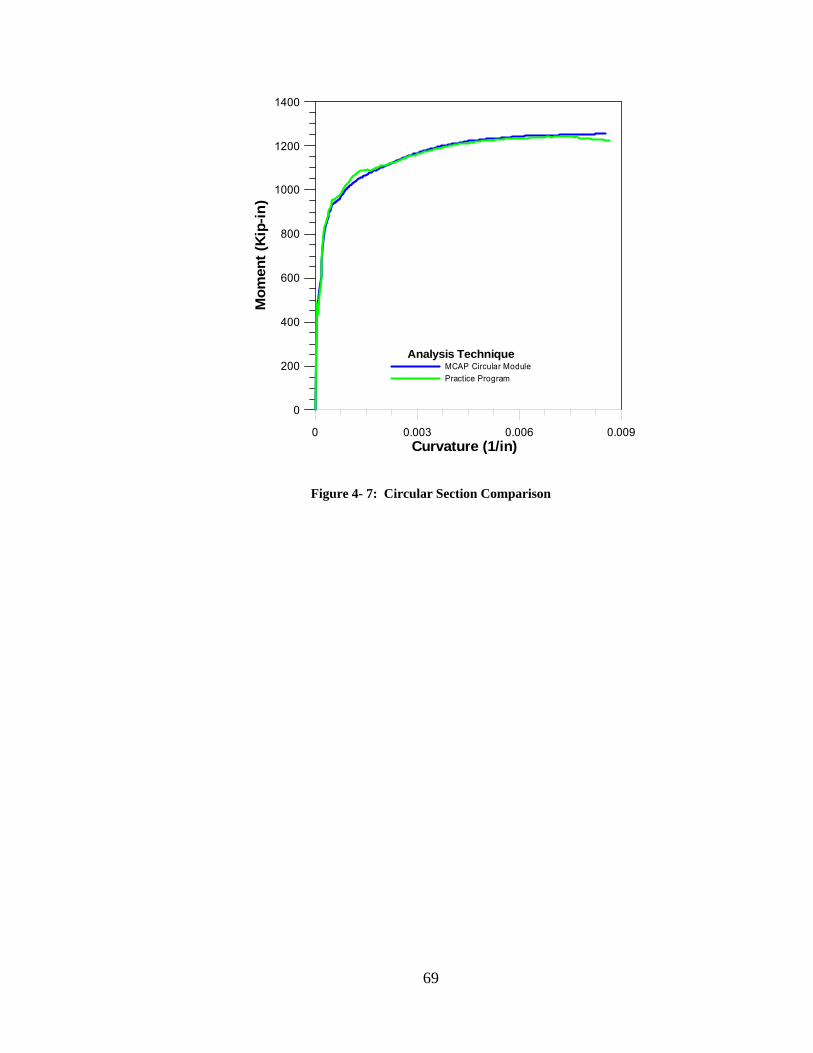
69

Figure 4- 7: Circular Section Comparison

0 0.003 0.006 0.009Curvature (1/in)

0

200

400

600

800

1000

1200

1400

Mo

men

t (K

ip-i

n)

Analysis TechniqueMCAP Circular Module

Practice Program

70

Chapter 5 - Conclusions in the Development of MCAP

MCAP is an effective program for generating M-φ relationships for RC

Sections. The program provides a useful interface for an OpenSees analysis

backbone and is user friendly. As a teaching aid, MCAP is accurate, uses

conventional material models and MCAP provides an advantage on modeling

user defined sections and rotated sections that were not possible with other

Moment-Curvature programs. There are a range of instructional applications

including learning about materials and structural analysis. The program is

versatile in this respect since it can be used equally well by undergraduates and

graduates. The development of MCAP has also provided insight as to how to

increase computational accuracy through the relationship between curvature and

the strain in the extreme reinforcing steel layer and decrease computational

times for all programs that are developed for M-φ analysis.

Future developments for MCAP include a pile analysis module and expanding

the program to perform a pushover analyses for reinforced concrete members.

The implementation of a FRP confined section module is also being developed

with an immediate application to the retrofit of circular and rectangular concrete

sections. Further research on the relationship between the curvature and the

strains in the extreme steel fibers is a future development that MCAP can help

accomplish. This relationship is valuable in Moment-Curvature analysis. If one

could define a relationship between curvature and the strain in the extreme steel

fiber for any section, the neutral axis could be easily defined for the analysis.

This would then result in Moment-Curvature analysis that could be performed by

71

hand calculations instead of an iterative process adapted to computer analysis.

A simplified hand analysis technique would be a great tool for engineers needing

the Moment-Curvature relationship.

72

References Bentz, Evan. 2011. “Download Response 2000.” Accessed January 15. http://www.ecf.utoronto.ca/~bentz/download.htm Bozorgnia, Yousef and Vitelmo V. Bertero. 2004. Earthquake Engineering From Engineering Seismology to Performance-Based Engineering. Boca Raton: CRC Press. Chandrasekaran, Srinivasan et al. 2010. Seismic Design Aids for Nonlinear Analysis of Reinforced Concrete Structures. Boca Raton: CRC Press. Chang, G. A. and J.B. Mander. “Seismic Energy Based Fatigue Damage Analysis of Bridge Columns: Part I – Evaluation of Seismic Capacity.” (Buffalo, NY: National Center for Earthquake Engineering Research, 1994) Kent, D. C. and R. Park. 1973. “Cyclic Load Behaviour of Reinforcing Steel.” Strain 9: 98–103. Accessed November 10, 2010. doi: 10.1111/j.1475-1305.1973.tb01816.x

Mander, J. B., M. J. N. Priestley and R. Park. 1988. Theoretical Stress-Strain Model for Confined Concrete. Journal of Structural Engineering. 114: 1804-1826.

Matthews, Robert. 2001. “Moment Curvature Analysis”. Accessed January 15, 2011. http://structsource.com/pdf/Momcurv_web.pdf Matthews, Robert, 2009. “Consec Program Information”. Accessed January 15, 2011. http://www.structware.com/consec/consec_home.html Mazzoni, Silvia and Frank McKenna. 2006. “Example 9. Moment-Curvature Analysis of Section.” Accessed January 15. 2011. http://opensees.berkeley.edu/OpenSees/manuals/ExamplesManual/HTML/3909.htm Mazzoni, Silvia et al. 2006. “OpenSees Command Language Manual.” Accessed January 15, 2011. http://opensees.berkeley.edu/OpenSees/manuals/usermanual/OpenSeesCommandLanguageManualJune2006.pdf Park, Robert and Thomas Paulay. 1975. Reinforced Concrete Structures. New York: John Wiley & Sons, Inc. Paulay, Thomas and M. J. N. Priestley. 1992. Seismic Design of Reinforced Concrete and Masonry Buildings. New York: John Wiley & Sons, Inc.

73

Penelis, George G. and Andreas J. Kappos. 1997. Earthquake-Resistant Concrete Structures. London: E&FN Spon. Priestley, M. J. N., Frieder Seible and Gian Michele Calvi. 1996. Seismic Design and Retrofit of Bridges. New York: John Wiley & Sons, Inc. Seismosoft. 2011. “Download”. Accessed January 15. http://www.seismosoft.com/en/Download.aspx Silva,P. F. et al. 1999. “Full-Scale Proof Test of the Alaska Cast-in-Place Steel Shell Three Column Bridge Bent Test, Report No. SSRP-98/13.” Department of Structural Engineering, University of California San Diego. The MathWorks, Inc. 2007. “windows_motion_test.m and draw_lines.m functions.” Accessed January 15, 2011. Available from Matlab Version 7 Help Index, Release 2007a

74

Appendix A – Rectangular Section Example *.tcl File

#Units: Kips, Inches, Seconds #------------------------------------------------------------------ wipe; file mkdir TEST_Rect_1; model BasicBuilder -ndm 3 -ndf 6; source LibUnits.tcl # define GEOMETRY #------------------------------------------------------------------ set LCol [expr 120*$in]; set Weight [expr -10*$kip]; # calculated parameters set PCol $Weight; # nodal dead-load weight per column # nodal coordinates: node 1 0 0 0 0 0 0; # Node#, X, Y node 3 0 0 0 0 0 0; set SecTag 1; # Single point constraints -- Boundary Conditions fix 1 1 1 1 1 1 1; # node DX DY RZ fix 3 0 1 1 1 0 1; # MATERIAL parameters #------------------------------------------------------------------ #------------Concrete-------------------- set IDconcCore 1; set IDconcCover 2; # nominal concrete compressive strength set fc [expr -5*$ksi]; set Ec [expr 57*$ksi*pow((-$fc/$psi),0.5)]; # confined concrete set Kfc 1.121; # ratio of confined to unconfined concrete strength set fc1C [expr $Kfc*$fc]; # CONFINED concrete (mander model), maximum stress set eps1C -0.0032099; # strain at maximum stress set xncon 7.0431; # Non-dimensional term that defines the strain at which the straight line descent begins in compression set rrcon 1.7644; # Parameter that controls the nonlinear descending branch # unconfined concrete set fc1U $fc; # UNCONFINED concrete (todeschini parabolic model), maximum stress set eps1U -0.002; # strain at maximum strength of unconfined concrete

75

set xnunc 2.3; # Non-dimensional term that defines the strain at which the straight line descent begins in compression set rrunc 4.7667; # Parameter that controls the nonlinear descending branch # tensile-strength properties set ftC 0.60458; # tensile strength +tension set ftU 0.60458; # tensile strength +tension set et 0.00015; # tensile strain at maximum tension stress set xp 2; # Non-dimensional term that defines the strain at which the straight line descent begins in tension #---------------Steel Reinforcement------------------ set IDreinf 3; # material ID tag -- reinforcement # Steel properties set Fy [expr 60*$ksi]; # STEEL yield stress set Fu [expr 90*$ksi]; # Ultimate STEEL yield stress set esh 0.00672; # strain at hardening set eult 0.12; # strain at ultimate set Es 29000; # modulus of steel set Esh 2200; # modulus of steel after hardening # build uniaxial material uniaxialMaterial ReinforcingSteel $IDreinf $Fy $Fu $Es $Esh $esh $eult; uniaxialMaterial Concrete07 $IDconcCore $fc1C $eps1C $Ec $ftC $et $xp $xncon $rrcon; # build core concrete (confined) uniaxialMaterial Concrete07 $IDconcCover $fc1U $eps1U $Ec $ftC $et $xp $xnunc $rrunc; # build cover concrete (unconfined) # FIBER SECTION properties #------------------------------------------------------------------ #RC Rectangular Section # Column section geometry set Depth [expr 16*$in]; # Column Depth set Width [expr 12*$in]; # Column Width set cover [expr 1*$in]; # Column cover to reinforcing steel set numBarsTop 4; # number of longitudinal-reinforcement TOP set numBarsBot 4; # number of longitudinal-reinforcement BOTTOM set numBarsIntTot 0; # Number of Side Bars (Total) set barAreaTop [expr 0.19635*$in2]; # area of longitudinal-reinforcement bars -- top set barAreaBot [expr 0.19635*$in2]; # area of longitudinal-reinforcement bars -- bot set barAreaInt [expr 0.7854*$in2]; # area of longitudinal-reinforcement bars -- intermediate skin reinf set TransDia [expr 0.375*$in]; # Dia of Trans-reinforcement bars set LongRad [expr 0.25*$in]; # Dia of Trans-reinforcement bars set SBspacing [expr 12.75*$in]; # Dia of Trans-reinforcement bars set SideRad [expr 0.5*$in]; # Dia of Trans-reinforcement bars set coverZ [expr $Depth/2.0]; # The distance from the section z-axis to the edge of the cover concrete -- outer edge of cover concrete set coverY [expr $Width/2.0]; # The distance from the section x-axis to the edge of the cover concrete -- outer edge of cover concrete

76

set coreZ [expr $coverZ-$cover]; # The distance from the section z-axis to the edge of the core concrete -- edge of the core concrete/inner edge of cover concrete set coreY [expr $coverY-$cover]; # The distance from the section x-axis to the edge of the core concrete -- edge of the core concrete/inner edge of cover concrete set coreY2 [expr $coverY-$cover-$TransDia/2-$LongRad]; set coreZ2 [expr $coverZ-$cover-$TransDia/2-$LongRad]; set coreZ3 [expr $coverZ-$cover-$TransDia/2-$LongRad-$SBspacing]; set coreY3 [expr $coverY-$cover-$TransDia/2-$SideRad]; set nfY 64; # number of fibers for concrete in Y-direction set nfZ 64; # number of fibers for concrete in z-direction set numBarsInt [expr $numBarsIntTot/2]; # number of intermediate bars per side section Fiber $SecTag {; # Define the fiber section patch quadr $IDconcCore $nfY $nfZ -5 -7 5 -7 5 7 -5 7; # Define the core patch patch quadr $IDconcCover 1 $nfZ -6 -8 -5 -8 -5 8 -6 8; # Define the four cover patches patch quadr $IDconcCover $nfY 1 -5 -8 5 -8 5 -7 -5 -7; patch quadr $IDconcCover 1 $nfZ 5 -8 6 -8 6 8 5 8; patch quadr $IDconcCover $nfY 1 -5 7 5 7 5 8 -5 8; layer straight $IDreinf $numBarsTop $barAreaTop -4.5625 -6.5625 4.5625 -6.5625; # top layer reinfocement layer straight $IDreinf $numBarsBot $barAreaBot -4.5625 6.5625 4.5625 6.5625; # bottom layer reinforcement }; # end of fibersection definition # Define element # tag ndI ndJ secTag element zeroLengthSection 1 1 3 $SecTag # Create recorder recorder Node -file TEST_Rect_1/TEST_Rect_1.out -time -node 3 -dof 5 disp; # output moment (col 1) & curvature (col 2) recorder Element -file TEST_Rect_1/TEST_Rect_12.out -time -ele 1 section fiber $coreY2 $coreZ2 $IDreinf stressStrain; recorder Element -file TEST_Rect_1/TEST_Rect_13.out -time -ele 1 section fiber [expr $coreY-1.5*2*$coreY/64] [expr -$coreZ+0.5*2*$coreZ/64] $IDconcCore stressStrain # Define constant axial load pattern Plain 1 "Constant" { load 3 $PCol 0.0 0.0 0.0 0.0 0.0 } # Define analysis parameters integrator LoadControl 0 1 0 0 system SparseGeneral -piv; # Overkill, but may need the pivoting! test NormUnbalance 1.0e-9 10 numberer RCM constraints Transformation

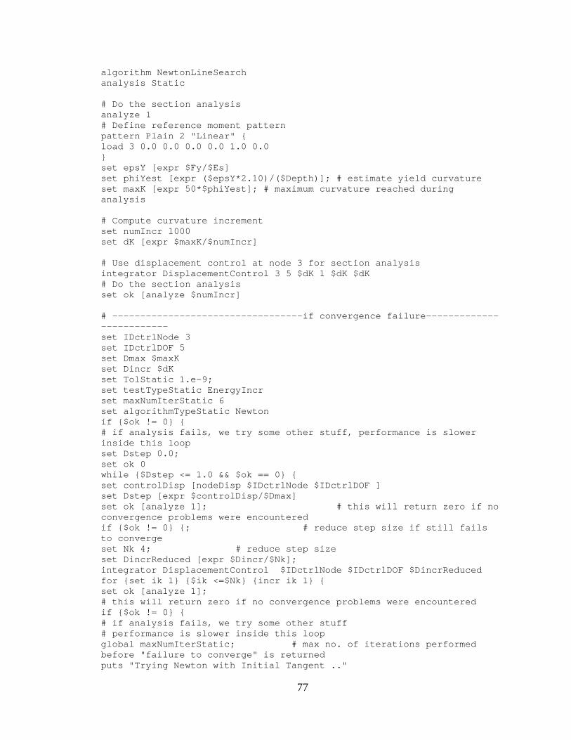
77

algorithm NewtonLineSearch analysis Static # Do the section analysis analyze 1 # Define reference moment pattern pattern Plain 2 "Linear" { load 3 0.0 0.0 0.0 0.0 1.0 0.0 } set epsY [expr $Fy/$Es] set phiYest [expr ($epsY*2.10)/($Depth)]; # estimate yield curvature set maxK [expr 50*$phiYest]; # maximum curvature reached during analysis # Compute curvature increment set numIncr 1000 set dK [expr $maxK/$numIncr] # Use displacement control at node 3 for section analysis integrator DisplacementControl 3 5 $dK 1 $dK $dK # Do the section analysis set ok [analyze $numIncr] # ----------------------------------if convergence failure------------------------- set IDctrlNode 3 set IDctrlDOF 5 set Dmax $maxK set Dincr $dK set TolStatic 1.e-9; set testTypeStatic EnergyIncr set maxNumIterStatic 6 set algorithmTypeStatic Newton if {$ok != 0} { # if analysis fails, we try some other stuff, performance is slower inside this loop set Dstep 0.0; set ok 0 while {$Dstep <= 1.0 && $ok == 0} { set controlDisp [nodeDisp $IDctrlNode $IDctrlDOF ] set Dstep [expr $controlDisp/$Dmax] set ok [analyze 1]; # this will return zero if no convergence problems were encountered if {$ok != 0} {; # reduce step size if still fails to converge set Nk 4; # reduce step size set DincrReduced [expr $Dincr/$Nk]; integrator DisplacementControl $IDctrlNode $IDctrlDOF $DincrReduced for {set ik 1} {$ik <=$Nk} {incr ik 1} { set ok [analyze 1]; # this will return zero if no convergence problems were encountered if {$ok != 0} { # if analysis fails, we try some other stuff # performance is slower inside this loop global maxNumIterStatic; # max no. of iterations performed before "failure to converge" is returned puts "Trying Newton with Initial Tangent .."

78

test NormDispIncr $TolStatic 2000 0 algorithm Newton -initial set ok [analyze 1] test $testTypeStatic $TolStatic $maxNumIterStatic 0 algorithm $algorithmTypeStatic } if {$ok != 0} { puts "Trying Broyden .." algorithm Broyden 8 set ok [analyze 1 ] algorithm $algorithmTypeStatic } if {$ok != 0} { puts "Trying NewtonWithLineSearch " algorithm NewtonLineSearch 0.8 set ok [analyze 1] algorithm $algorithmTypeStatic } if {$ok != 0} {; # stop if still fails to converge puts [format $fmt1 "PROBLEM" $IDctrlNode $IDctrlDOF [nodeDisp $IDctrlNode $IDctrlDOF] $LunitTXT] return -1 }; # end if }; # end for integrator DisplacementControl $IDctrlNode $IDctrlDOF $Dincr; # bring back to original increment }; # end if }; # end while loop }; # end if ok !0 # -------------------------------------------------------------------- global LunitTXT; # load time-unit text if { [info exists LunitTXT] != 1} {set LunitTXT "Length"}; # set blank if it has not been defined previously. set fmt1 "%s Pushover analysis: CtrlNode %.3i, dof %.1i, Curv=%.4f /%s"; # format for screen/file output of DONE/PROBLEM analysis if {$ok != 0 } { puts [format $fmt1 "PROBLEM" $IDctrlNode $IDctrlDOF [nodeDisp $IDctrlNode $IDctrlDOF] $LunitTXT] } else { puts [format $fmt1 "DONE" $IDctrlNode $IDctrlDOF [nodeDisp $IDctrlNode $IDctrlDOF] $LunitTXT] }

79

Appendix B – Circular Section Example *.tcl File

#Units: Kips, Inches, Seconds #------------------------------------------------------------------ wipe; file mkdir Test_Circ_1; model BasicBuilder -ndm 3 -ndf 6; source LibUnits.tcl # define GEOMETRY #------------------------------------------------------------------ set LCol [expr 120*$in]; set Weight [expr -10*$kip]; # calculated parameters set PCol $Weight; # nodal dead-load weight per column # nodal coordinates: node 1 0 0 0 0 0 0; # Node#, X, Y node 3 0 0 0 0 0 0; set SecTag 1; # Single point constraints -- Boundary Conditions fix 1 1 1 1 1 1 1; # node DX DY RZ fix 3 0 1 1 1 0 1; # MATERIAL parameters #------------------------------------------------------------------ #------------Concrete-------------------- set IDconcCore 1; set IDconcCover 2; # nominal concrete compressive strength set fc [expr -5*$ksi]; set Ec [expr 57*$ksi*pow((-$fc/$psi),0.5)]; # confined concrete set Kfc 1.3627; # ratio of confined to unconfined concrete strength set fc1C [expr $Kfc*$fc]; # CONFINED concrete (mander model), maximum stress set eps1C -0.0056266; # strain at maximum stress set xncon 3.5529; # Non-dimensional term that defines the strain at which the straight line descent begins in compression set rrcon 1.4295; # Parameter that controls the nonlinear descending branch # unconfined concrete set fc1U $fc; # UNCONFINED concrete (todeschini parabolic model), maximum stress set eps1U -0.002; # strain at maximum strength of unconfined concrete

80

set xnunc 2.3; # Non-dimensional term that defines the strain at which the straight line descent begins in compression set rrunc 4.7667; # Parameter that controls the nonlinear descending branch # tensile-strength properties set ftC 0.60458; # tensile strength +tension set ftU 0.60458; # tensile strength +tension set et 0.00015; # tensile strain at maximum tension stress set xp 2; # Non-dimensional term that defines the strain at which the straight line descent begins in tension #---------------Steel Reinforcement------------------ set IDreinf 3; # material ID tag -- reinforcement # Steel properties set Fy [expr 60*$ksi]; # STEEL yield stress set Fu [expr 90*$ksi]; # Ultimate STEEL yield stress set esh 0.00672; # strain at hardening set eult 0.12; # strain at ultimate set Es 29000; # modulus of steel set Esh 2200; # modulus of steel after hardening # build uniaxial material uniaxialMaterial ReinforcingSteel $IDreinf $Fy $Fu $Es $Esh $esh $eult; uniaxialMaterial Concrete07 $IDconcCore $fc1C $eps1C $Ec $ftC $et $xp $xncon $rrcon; # build core concrete (confined) uniaxialMaterial Concrete07 $IDconcCover $fc1U $eps1U $Ec $ftC $et $xp $xnunc $rrunc; # build cover concrete (unconfined) # FIBER SECTION properties #------------------------------------------------------------------ #RC Circular Section # Column section geometry set cover [expr 1*$in]; # Column cover to reinforcing steel set numBars 8; # number of longitudinal-reinforcement set barArea [expr 0.3068*$in2]; # area of longitudinal-reinforcement bars -- top set TransDia [expr 0.375*$in]; # Dia of Trans-reinforcement bars set SteelRad [expr 6.5*$in]; # Rad of Long-reinforcement bars Layer set CoreRad [expr 7*$in]; # Rad of Conc. Core set OuterRad [expr 8*$in]; # Rad of Column set OuterDia [expr 16*$in]; # DIA of Column set nfr 48; # number of fibers for concrete in radius set nfc 32; # number of fibers for concrete in circlular direction section Fiber $SecTag {; # Define the fiber section patch circ $IDconcCore $nfc $nfr 0 0 0 $CoreRad 0 360; # Define the core patch patch circ $IDconcCover $nfc $nfr 0 0 $CoreRad $OuterRad 180 472.5; # Define the cover patch layer circ $IDreinf $numBars $barArea 0 0 $SteelRad; # Steel Layer }; # end of fibersection definition

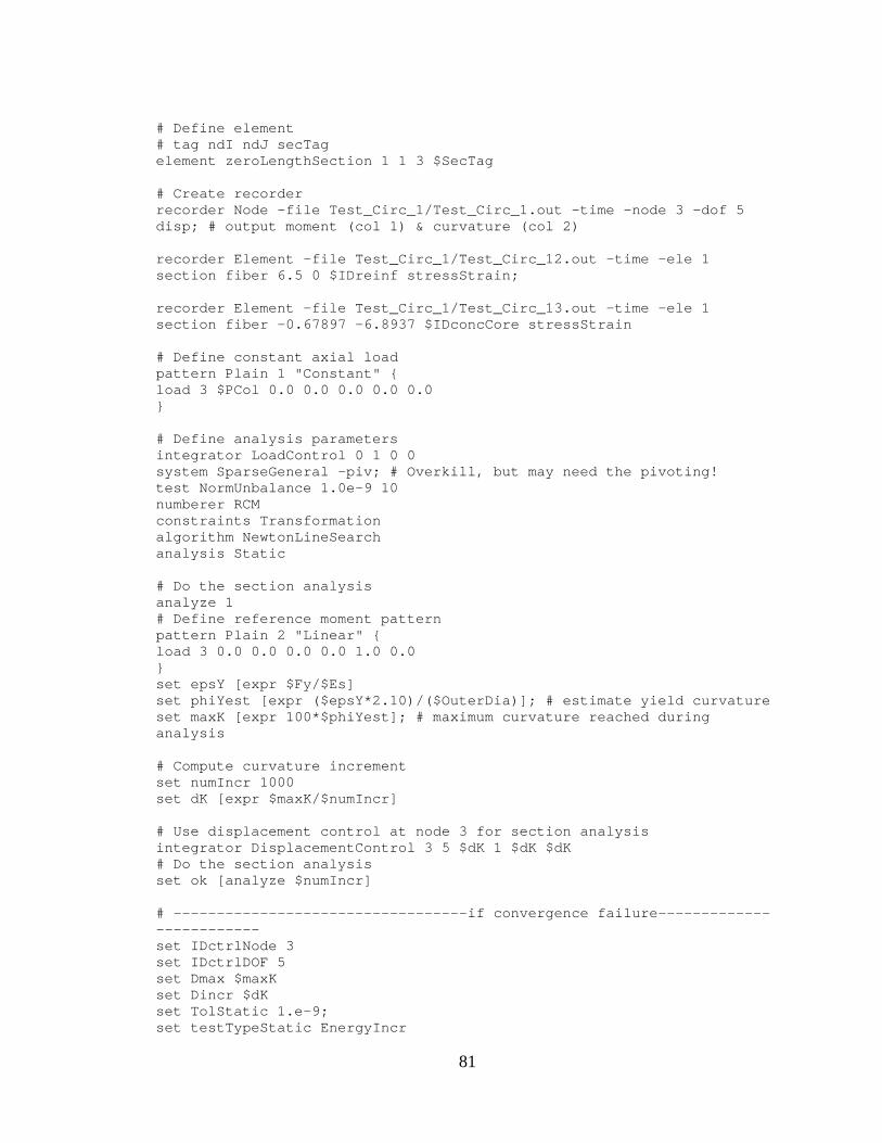
81

# Define element # tag ndI ndJ secTag element zeroLengthSection 1 1 3 $SecTag # Create recorder recorder Node -file Test_Circ_1/Test_Circ_1.out -time -node 3 -dof 5 disp; # output moment (col 1) & curvature (col 2) recorder Element -file Test_Circ_1/Test_Circ_12.out -time -ele 1 section fiber 6.5 0 $IDreinf stressStrain; recorder Element -file Test_Circ_1/Test_Circ_13.out -time -ele 1 section fiber -0.67897 -6.8937 $IDconcCore stressStrain # Define constant axial load pattern Plain 1 "Constant" { load 3 $PCol 0.0 0.0 0.0 0.0 0.0 } # Define analysis parameters integrator LoadControl 0 1 0 0 system SparseGeneral -piv; # Overkill, but may need the pivoting! test NormUnbalance 1.0e-9 10 numberer RCM constraints Transformation algorithm NewtonLineSearch analysis Static # Do the section analysis analyze 1 # Define reference moment pattern pattern Plain 2 "Linear" { load 3 0.0 0.0 0.0 0.0 1.0 0.0 } set epsY [expr $Fy/$Es] set phiYest [expr ($epsY*2.10)/($OuterDia)]; # estimate yield curvature set maxK [expr 100*$phiYest]; # maximum curvature reached during analysis # Compute curvature increment set numIncr 1000 set dK [expr $maxK/$numIncr] # Use displacement control at node 3 for section analysis integrator DisplacementControl 3 5 $dK 1 $dK $dK # Do the section analysis set ok [analyze $numIncr] # ----------------------------------if convergence failure------------------------- set IDctrlNode 3 set IDctrlDOF 5 set Dmax $maxK set Dincr $dK set TolStatic 1.e-9; set testTypeStatic EnergyIncr

82

set maxNumIterStatic 6 set algorithmTypeStatic Newton if {$ok != 0} { # if analysis fails, we try some other stuff, performance is slower inside this loop set Dstep 0.0; set ok 0 while {$Dstep <= 1.0 && $ok == 0} { set controlDisp [nodeDisp $IDctrlNode $IDctrlDOF ] set Dstep [expr $controlDisp/$Dmax] set ok [analyze 1]; # this will return zero if no convergence problems were encountered if {$ok != 0} {; # reduce step size if still fails to converge set Nk 4; # reduce step size set DincrReduced [expr $Dincr/$Nk]; integrator DisplacementControl $IDctrlNode $IDctrlDOF $DincrReduced for {set ik 1} {$ik <=$Nk} {incr ik 1} { set ok [analyze 1]; # this will return zero if no convergence problems were encountered if {$ok != 0} { # if analysis fails, we try some other stuff # performance is slower inside this loop global maxNumIterStatic; # max no. of iterations performed before "failure to converge" is returned puts "Trying Newton with Initial Tangent .." test NormDispIncr $TolStatic 2000 0 algorithm Newton -initial set ok [analyze 1] test $testTypeStatic $TolStatic $maxNumIterStatic 0 algorithm $algorithmTypeStatic } if {$ok != 0} { puts "Trying Broyden .." algorithm Broyden 8 set ok [analyze 1 ] algorithm $algorithmTypeStatic } if {$ok != 0} { puts "Trying NewtonWithLineSearch " algorithm NewtonLineSearch 0.8 set ok [analyze 1] algorithm $algorithmTypeStatic } if {$ok != 0} {; # stop if still fails to converge puts [format $fmt1 "PROBLEM" $IDctrlNode $IDctrlDOF [nodeDisp $IDctrlNode $IDctrlDOF] $LunitTXT] return -1 }; # end if }; # end for integrator DisplacementControl $IDctrlNode $IDctrlDOF $Dincr; # bring back to original increment }; # end if }; # end while loop }; # end if ok !0 # -------------------------------------------------------------------- global LunitTXT; # load time-unit text

83

if { [info exists LunitTXT] != 1} {set LunitTXT "Length"}; # set blank if it has not been defined previously. set fmt1 "%s Pushover analysis: CtrlNode %.3i, dof %.1i, Curv=%.4f /%s"; # format for screen/file output of DONE/PROBLEM analysis if {$ok != 0 } { puts [format $fmt1 "PROBLEM" $IDctrlNode $IDctrlDOF [nodeDisp $IDctrlNode $IDctrlDOF] $LunitTXT] } else { puts [format $fmt1 "DONE" $IDctrlNode $IDctrlDOF [nodeDisp $IDctrlNode $IDctrlDOF] $LunitTXT] }

84

Appendix C – User Defined Section Example *.tcl File

#Units: Kips, Inches, Seconds #------------------------------------------------------------------ wipe; file mkdir UD_Example; model BasicBuilder -ndm 3 -ndf 6; source LibUnits.tcl # define GEOMETRY #------------------------------------------------------------------ set LCol [expr 120*$in]; set Weight [expr -10*$kip]; # calculated parameters set PCol $Weight; # nodal dead-load weight per column set Depth [expr 23.36*$in]; # nodal coordinates: node 1 0 0 0 0 0 0; # Node#, X, Y node 3 0 0 0 0 0 0; set SecTag 1; # Single point constraints -- Boundary Conditions fix 1 1 1 1 1 1 1; # node DX DY RZ fix 3 0 1 1 1 0 1; # MATERIAL parameters #------------------------------------------------------------------ #------------Concrete-------------------- set IDconcCore 1; set IDconcCover 2; # nominal concrete compressive strength set fc [expr -5*$ksi]; set Ec [expr 57*$ksi*pow((-$fc/$psi),0.5)]; # confined concrete set Kfc 1.1941; # ratio of confined to unconfined concrete strength set fc1C [expr $Kfc*$fc]; # CONFINED concrete (mander model), maximum stress set eps1C -0.0039413; # strain at maximum stress set xncon 7.8225; # Non-dimensional term that defines the strain at which the straight line descent begins in compression set rrcon 1.6022; # Parameter that controls the nonlinear descending branch # unconfined concrete set fc1U $fc; # UNCONFINED concrete (todeschini parabolic model), maximum stress

85

set eps1U -0.002; # strain at maximum strength of unconfined concrete set xnunc 2.3; # Non-dimensional term that defines the strain at which the straight line descent begins in compression set rrunc 4.7667; # Parameter that controls the nonlinear descending branch # tensile-strength properties set ftC 0.60458; # tensile strength +tension set ftU 0.60458; # tensile strength +tension set et 0.00015; # tensile strain at maximum tension stress set xp 2; # Non-dimensional term that defines the strain at which the straight line descent begins in tension #---------------Steel Reinforcement------------------ set IDreinf 3; # material ID tag -- reinforcement # Steel properties set Fy [expr 60*$ksi]; # STEEL yield stress set Fu [expr 90*$ksi]; # Ultimate STEEL yield stress set esh 0.00672; # strain at hardening set eult 0.12; # strain at ultimate set Es 29000; # modulus of steel set Esh 2200; # modulus of steel after hardening # build uniaxial material uniaxialMaterial ReinforcingSteel $IDreinf $Fy $Fu $Es $Esh $esh $eult; uniaxialMaterial Concrete07 $IDconcCore $fc1C $eps1C $Ec $ftC $et $xp $xncon $rrcon; # build core concrete (confined) uniaxialMaterial Concrete07 $IDconcCover $fc1U $eps1U $Ec $ftC $et $xp $xnunc $rrunc; # build cover concrete (unconfined) # FIBER SECTION properties #------------------------------------------------------------------ #RC Rectangular Section # Column section geometry section Fiber $SecTag {; # Define the fiber section fiber 7.7867 11.68 0.1536 $IDconcCover fiber 7.7867 11.36 0.068267 $IDconcCover fiber 7.7867 11.04 0.068267 $IDconcCover fiber 7.7867 10.72 0.068267 $IDconcCover fiber 7.7867 10.4 0.068267 $IDconcCover fiber 7.7867 10.08 0.068267 $IDconcCover fiber 7.7867 9.76 0.068267 $IDconcCover fiber 7.7867 9.44 0.068267 $IDconcCover fiber 7.7867 9.12 0.068267 $IDconcCover fiber 7.7867 8.8 0.068267 $IDconcCover fiber 7.7867 8.48 0.068267 $IDconcCover fiber 7.7867 8.16 0.068267 $IDconcCover fiber 7.7867 7.84 0.068267 $IDconcCover fiber 7.7867 7.52 0.068267 $IDconcCover fiber 7.7867 7.2 0.068267 $IDconcCover fiber 7.7867 6.88 0.068267 $IDconcCover fiber 7.7867 6.56 0.068267 $IDconcCover

86

fiber 7.7867 6.24 0.068267 $IDconcCover fiber 7.7867 5.92 0.068267 $IDconcCover fiber 7.7867 -5.92 0.068267 $IDconcCover fiber 7.7867 -6.24 0.068267 $IDconcCover fiber 7.7867 -6.56 0.068267 $IDconcCover fiber 7.7867 -6.88 0.068267 $IDconcCover fiber 7.7867 -7.2 0.068267 $IDconcCover fiber 7.7867 -7.52 0.068267 $IDconcCover fiber 7.7867 -7.84 0.068267 $IDconcCover fiber 7.7867 -8.16 0.068267 $IDconcCover fiber 7.7867 -8.48 0.068267 $IDconcCover fiber 7.7867 -8.8 0.068267 $IDconcCover fiber 7.7867 -9.12 0.068267 $IDconcCover fiber 7.7867 -9.44 0.068267 $IDconcCover fiber 7.7867 -9.76 0.068267 $IDconcCover fiber 7.7867 -10.08 0.068267 $IDconcCover fiber 7.7867 -10.4 0.068267 $IDconcCover fiber 7.7867 -10.72 0.068267 $IDconcCover fiber 7.7867 -11.04 0.068267 $IDconcCover fiber 7.7867 -11.36 0.068267 $IDconcCover fiber 7.7867 -11.68 0.1536 $IDconcCover fiber 7.5733 11.68 0.1024 $IDconcCover fiber 7.5733 11.36 0.068267 $IDconcCover fiber 7.5733 11.04 0.068267 $IDconcCover fiber 7.5733 10.72 0.068267 $IDconcCover fiber 7.5733 10.4 0.068267 $IDconcCover fiber 7.5733 10.08 0.068267 $IDconcCover fiber 7.5733 9.76 0.068267 $IDconcCover fiber 7.5733 9.44 0.068267 $IDconcCover fiber 7.5733 9.12 0.068267 $IDconcCover fiber 7.5733 8.8 0.068267 $IDconcCover fiber 7.5733 8.48 0.068267 $IDconcCover fiber 7.5733 8.16 0.068267 $IDconcCover fiber 7.5733 7.84 0.068267 $IDconcCover fiber 7.5733 7.52 0.068267 $IDconcCover fiber 7.5733 7.2 0.068267 $IDconcCover fiber 7.5733 6.88 0.068267 $IDconcCover fiber 7.5733 6.56 0.068267 $IDconcCover fiber 7.5733 6.24 0.068267 $IDconcCover fiber 7.5733 5.92 0.068267 $IDconcCover fiber 7.5733 -5.92 0.068267 $IDconcCover fiber 7.5733 -6.24 0.068267 $IDconcCover fiber 7.5733 -6.56 0.068267 $IDconcCover fiber 7.5733 -6.88 0.068267 $IDconcCover fiber 7.5733 -7.2 0.068267 $IDconcCover fiber 7.5733 -7.52 0.068267 $IDconcCover fiber 7.5733 -7.84 0.068267 $IDconcCover fiber 7.5733 -8.16 0.068267 $IDconcCover fiber 7.5733 -8.48 0.068267 $IDconcCover fiber 7.5733 -8.8 0.068267 $IDconcCover fiber 7.5733 -9.12 0.068267 $IDconcCover fiber 7.5733 -9.44 0.068267 $IDconcCover fiber 7.5733 -9.76 0.068267 $IDconcCover fiber 7.5733 -10.08 0.068267 $IDconcCover fiber 7.5733 -10.4 0.068267 $IDconcCover fiber 7.5733 -10.72 0.068267 $IDconcCover fiber 7.5733 -11.04 0.068267 $IDconcCover

87

------ Pages of the Fiber Definition have been omitted for brevity---- fiber 6.8133 10.7067 0.1232 $IDconcCore fiber 6.8133 10.4133 0.054756 $IDconcCore fiber 6.8133 10.12 0.054756 $IDconcCore fiber 6.8133 9.8267 0.054756 $IDconcCore fiber 6.8133 9.5333 0.054756 $IDconcCore fiber 6.8133 9.24 0.054756 $IDconcCore fiber 6.8133 8.9467 0.054756 $IDconcCore fiber 6.8133 8.6533 0.054756 $IDconcCore fiber 6.8133 8.36 0.054756 $IDconcCore fiber 6.8133 8.0667 0.054756 $IDconcCore fiber 6.8133 7.7733 0.054756 $IDconcCore fiber 6.8133 7.48 0.054756 $IDconcCore fiber 6.8133 7.1867 0.054756 $IDconcCore fiber 6.8133 -7.1867 0.054756 $IDconcCore fiber 6.8133 -7.48 0.054756 $IDconcCore fiber 6.8133 -7.7733 0.054756 $IDconcCore fiber 6.8133 -8.0667 0.054756 $IDconcCore fiber 6.8133 -8.36 0.054756 $IDconcCore fiber 6.8133 -8.6533 0.054756 $IDconcCore fiber 6.8133 -8.9467 0.054756 $IDconcCore fiber 6.8133 -9.24 0.054756 $IDconcCore fiber 6.8133 -9.5333 0.054756 $IDconcCore fiber 6.8133 -9.8267 0.054756 $IDconcCore fiber 6.8133 -10.12 0.054756 $IDconcCore fiber 6.8133 -10.4133 0.054756 $IDconcCore fiber 6.8133 -10.7067 0.1232 $IDconcCore fiber 6.6267 10.7067 0.082133 $IDconcCore fiber 6.6267 10.4133 0.054756 $IDconcCore fiber 6.6267 10.12 0.054756 $IDconcCore fiber 6.6267 9.8267 0.054756 $IDconcCore fiber 6.6267 9.5333 0.054756 $IDconcCore fiber 6.6267 9.24 0.054756 $IDconcCore fiber 6.6267 8.9467 0.054756 $IDconcCore fiber 6.6267 8.6533 0.054756 $IDconcCore fiber 6.6267 8.36 0.054756 $IDconcCore fiber 6.6267 8.0667 0.054756 $IDconcCore fiber 6.6267 7.7733 0.054756 $IDconcCore fiber 6.6267 7.48 0.054756 $IDconcCore fiber 6.6267 7.1867 0.054756 $IDconcCore fiber 6.6267 6.8933 0.054756 $IDconcCore fiber 6.6267 -6.8933 0.054756 $IDconcCore fiber 6.6267 -7.1867 0.054756 $IDconcCore fiber 6.6267 -7.48 0.054756 $IDconcCore fiber 6.6267 -7.7733 0.054756 $IDconcCore fiber 6.6267 -8.0667 0.054756 $IDconcCore fiber 6.6267 -8.36 0.054756 $IDconcCore fiber 6.6267 -8.6533 0.054756 $IDconcCore fiber 6.6267 -8.9467 0.054756 $IDconcCore fiber 6.6267 -9.24 0.054756 $IDconcCore fiber 6.6267 -9.5333 0.054756 $IDconcCore fiber 6.6267 -9.8267 0.054756 $IDconcCore fiber 6.6267 -10.12 0.054756 $IDconcCore fiber 6.6267 -10.4133 0.054756 $IDconcCore fiber 6.6267 -10.7067 0.082133 $IDconcCore

88

------ Pages of the Fiber Definition have been omitted for brevity---- fiber 6 10.5 0.44179 $IDreinf fiber 2 10.5 0.44179 $IDreinf fiber -2 10.5 0.44179 $IDreinf fiber -6 10.5 0.44179 $IDreinf fiber -6 -10.5 0.44179 $IDreinf fiber -2 -10.5 0.44179 $IDreinf fiber 2 -10.5 0.44179 $IDreinf fiber 6 -10.5 0.44179 $IDreinf }; # end of fibersection definition # Define element # tag ndI ndJ secTag element zeroLengthSection 1 1 3 $SecTag # Create recorder recorder Node -file UD_Example/UD_Example.out -time -node 3 -dof 5 disp; # output moment (col 1) & curvature (col 2) recorder Element -file UD_Example/UD_Example2.out -time -ele 1 section fiber 6 10.5 $IDreinf stressStrain; recorder Element -file UD_Example/UD_Example3.out -time -ele 1 section fiber 6.8133 -10.7067 $IDconcCore stressStrain # Define constant axial load pattern Plain 1 "Constant" { load 3 $PCol 0.0 0.0 0.0 0.0 0.0 } # Define analysis parameters integrator LoadControl 0 1 0 0 system SparseGeneral -piv; # Overkill, but may need the pivoting! test NormUnbalance 1.0e-9 10 numberer RCM constraints Transformation algorithm NewtonLineSearch analysis Static # Do the section analysis analyze 1 # Define reference moment pattern pattern Plain 2 "Linear" { load 3 0.0 0.0 0.0 0.0 1.0 0.0 } set epsY [expr $Fy/$Es] set phiYest [expr ($epsY*2.10)/($Depth)]; # estimate yield curvature set maxK [expr 50*$phiYest]; # maximum curvature reached during analysis # Compute curvature increment set numIncr 1000 set dK [expr $maxK/$numIncr]

89

# Use displacement control at node 3 for section analysis integrator DisplacementControl 3 5 $dK 1 $dK $dK # Do the section analysis set ok [analyze $numIncr] # ----------------------------------if convergence failure------------ set IDctrlNode 3 set IDctrlDOF 5 set Dmax $maxK set Dincr $dK set TolStatic 1.e-9; set testTypeStatic EnergyIncr set maxNumIterStatic 6 set algorithmTypeStatic Newton if {$ok != 0} { # if analysis fails, we try some other stuff, performance is slower inside this loop set Dstep 0.0; set ok 0 while {$Dstep <= 1.0 && $ok == 0} { set controlDisp [nodeDisp $IDctrlNode $IDctrlDOF ] set Dstep [expr $controlDisp/$Dmax] set ok [analyze 1]; # this will return zero if no convergence problems were encountered if {$ok != 0} {; # reduce step size if still fails to converge set Nk 4; # reduce step size set DincrReduced [expr $Dincr/$Nk]; integrator DisplacementControl $IDctrlNode $IDctrlDOF $DincrReduced for {set ik 1} {$ik <=$Nk} {incr ik 1} { set ok [analyze 1]; # this will return zero if no convergence problems were encountered if {$ok != 0} { # if analysis fails, we try some other stuff # performance is slower inside this loop global maxNumIterStatic; # max no. of iterations performed before "failure to converge" is returned puts "Trying Newton with Initial Tangent .." test NormDispIncr $TolStatic 2000 0 algorithm Newton -initial set ok [analyze 1] test $testTypeStatic $TolStatic $maxNumIterStatic 0 algorithm $algorithmTypeStatic } if {$ok != 0} { puts "Trying Broyden .." algorithm Broyden 8 set ok [analyze 1 ] algorithm $algorithmTypeStatic } if {$ok != 0} { puts "Trying NewtonWithLineSearch " algorithm NewtonLineSearch 0.8 set ok [analyze 1] algorithm $algorithmTypeStatic } if {$ok != 0} {; # stop if still fails to converge

90

puts [format $fmt1 "PROBLEM" $IDctrlNode $IDctrlDOF [nodeDisp $IDctrlNode $IDctrlDOF] $LunitTXT] return -1 }; # end if }; # end for integrator DisplacementControl $IDctrlNode $IDctrlDOF $Dincr; # bring back to original increment }; # end if }; # end while loop }; # end if ok !0 # -------------------------------------------------------------------- global LunitTXT; # load time-unit text if { [info exists LunitTXT] != 1} {set LunitTXT "Length"}; # set blank if it has not been defined previously. set fmt1 "%s Pushover analysis: CtrlNode %.3i, dof %.1i, Curv=%.4f /%s"; # format for screen/file output of DONE/PROBLEM analysis if {$ok != 0 } { puts [format $fmt1 "PROBLEM" $IDctrlNode $IDctrlDOF [nodeDisp $IDctrlNode $IDctrlDOF] $LunitTXT] } else { puts [format $fmt1 "DONE" $IDctrlNode $IDctrlDOF [nodeDisp $IDctrlNode $IDctrlDOF] $LunitTXT] }

91

Appendix D – Rectangular Practice Program

The following sections detail the functions required for the rectangular

practice program. The circular program is similar, but takes into account the

circular geometry.

“main function”

function main() global fy Es Height inc Numinc dx1 dx2 Width cover NUMTB NUMBB Rowside SZTB SZBB DIVCT DIVCB DIVCC TB BB SB phi na DIVTB SZTRANS DIVBB Strain coordinates(); % Call Subroutine phiy=(fy/Es)*2.10/Height; % Estimate Yield Curvature phiinc=phiy/10; % Increment of Phi, Curvature dx3=1/300; % # Divisions TOL=2.5; phi=0; % Initial Value of Phi %--------Set Intitial Values of Compression, Tension and Moment to Zero C1=0; C2=0; C3=0; C4=0; C5=0; C6=0; C7=0; T1=0; T2=0; T3=0; T4=0; T5=0; T6=0; T7=0; C1x=0; C2x=0; C3x=0; C4x=0; C5x=0; C6x=0; C7x=0; T1x=0; T2x=0; T3x=0; T4x=0; T5x=0;

92

T6x=0; T7x=0; Cx=0; Tx=0; for j=1:147 % Number of increments = 147 if j==1 Moment(1,1)=0; % Start Point for M, Phi and Max Strain in Tensile Layer Curvature(1,1)=0; phi=phi+phiinc; MaxTen(1,1)=0; end if j==1 || j==2 % Adjust Tolerance for first two steps TOL=1.5; end if j==1 %Define Neutral Axis na=-Height/4; end if j==2 na=0; end %if j==3 % na=2; %end %if j==4 % na=2.5; %end if j>2 XYZ=MaxTen((j-1),1)*phi/Curvature((j-1),1); % Use Linear Relationship Between Strain and dist=-XYZ/phi; %curvature to define Neutral Axis for Current Step. na=dist-6.6733-.18; end % if j==5 % na=4; % end

93

% Find initial Forces for Given Phi [st1, st2, st3, st4, st5, st6]=strain(phi,na); % Find Strains for Discretization [f1, f2, f3, f4, f5, f6, f7] = stress(st1,st2,st3,st4, st5, st6); % Find Stresses for Discretization for i=1:inc forcecovT(i,1)=Width*dx2*(f1(i,1)+f1((i+1),1))/2; % Force in Cover Layers Top forcecovB(i,1)=Width*dx2*(f2(i,1)+f2((i+1),1))/2; % Force in Cover Layers Bottom xbarT(i,1)=(DIVCT(i,1)+DIVCT((i+1),1))/2; % Fiber Centroid top cover xbarB(i,1)=(DIVCB(i,1)+DIVCB((i+1),1))/2; % Fiber Centroid Bottom Cover if forcecovT(i,1)>0 C1=C1+forcecovT(i,1); % Force in Cover Top if Compression C1x=C1x+forcecovT(i,1)*xbarT(i,1); % Moment in Cover Top if compression end if forcecovT(i,1)<=0 T1=T1+forcecovT(i,1); % Force in Cover Top if Tension T1x=T1x+forcecovT(i,1)*xbarT(i,1); % Moment in Cover Top if Tension end if forcecovB(i,1)>0 C2=C2+forcecovB(i,1); % Force in Cover Bottom if Compression C2x=C2x+forcecovB(i,1)*xbarB(i,1); % moment in Cover Bottom if Compression end if forcecovB(i,1)<=0 T2=T2+forcecovB(i,1); % Force in Cover Bottom if Tension T2x=T2x+forcecovB(i,1)*xbarB(i,1); % Moment in Cover Bottom if Tension end end %-------------------Forces and Moments in Core Concrete Divisions for i=1:Numinc forceconf(i,1)=(Width-2*cover)*dx1*(f3(i,1)+f3((i+1),1))/2; forceunconf(i,1)=(2*cover)*dx1*(f4(i,1)+f4((i+1),1))/2; xbarConf(i,1)=(DIVCC(i,1)+DIVCC((i+1),1))/2; xbarUnConf(i,1)=(DIVCC(i,1)+DIVCC((i+1),1))/2; if forceconf(i,1)>0 C3=C3+forceconf(i,1); C3x=C3x+forceconf(i,1)*xbarConf(i,1); end if forceconf(i,1)<=0 T3=T3+forceconf(i,1);

94

T3x=T3x+forceconf(i,1)*xbarConf(i,1); end if forceunconf(i,1)>0 C4=C4+forceunconf(i,1); C4x=C4x+forceunconf(i,1)*xbarUnConf(i,1); end if forceunconf(i,1)<=0 T4=T4+forceunconf(i,1); T4x=T4x+forceunconf(i,1)*xbarUnConf(i,1); end end %-------Forces and Moments in Reinforcing %Layers--Bars are divided up into fibers--- for i=1:Numinc L=abs(TB(1,2)-DIVTB(i,1)); r=SZTB/16; CHDLGN=2*abs((r^2-L^2)^0.5); % Top Bars forcetb(i,1)=NUMTB*(f5(i,1)+f5((i+1),1))/2*dx1*CHDLGN; xbarTB=(DIVTB(i,1)+DIVTB((i+1),1))/2; if forcetb(i,1)>0 C5=C5+forcetb(i,1); C5x=C5x+forcetb(i,1)*xbarTB; end if forcetb<=0 T5=T5+forcetb(i,1); T5x=T5x+forcetb(i,1)*xbarTB; end end for i=1:Numinc L=abs(BB(1,2)-DIVBB(i,1)); r=SZBB/16; CHDLGN=2*abs((r^2-L^2)^0.5); % Bottom Bars forcebb(i,1)=NUMBB*(f6(i,1)+f6((i+1),1))/2*dx1*CHDLGN; xbarBB=(DIVBB(i,1)+DIVBB((i+1),1))/2; if forcebb(i,1)>0 C6=C6+forcebb(i,1); C6x=C6x+forcebb(i,1)*xbarBB; end if forcebb<=0 T6=T6+forcebb(i,1); T6x=T6x+forcebb(i,1)*xbarBB; end

95

end if Rowside~=0 for i=1:Rowside % Side Bars forcesb(i,1)=2*f7(i,1)*(SZSB/16)^2*pi(); if forcesb(i,1)>0 C7=C7+forcesb(i,1); C7x=C7x+forcesb(i,1)*(SB(i,3)); end if forcesb(i,1)<=0 T7=T7+forcesb(i,1); T7x=T7x+forcesb(i,1)*(SB(i,3)); end end else forcesb=0; end % Iterate until Compression and Tension Internal Forces are in Balance for k=1:((Height/2-na)/dx3-(cover+SZTRANS/16)/dx3)%Height/(2*dx3) Delta(k,1)=(C1+C2+C3+C4+C5+C6+C7+T1+T2+T3+T4+T5+T6+T7-10); C=C1+C2+C3+C4+C5+C6+C7-10; T=T1+T2+T3+T4+T5+T6+T7; if abs(C+T)>=TOL % if Greater than Tolerance of Balance dna(k,1)=dx3; % Incremental Change of Neutral Axis else if abs(Delta(k,1))<TOL % if Less than Tolerance dna(k,1)=0; % Stop increment break % Leave loop end end na=na+dna(k,1); % Increment neutral Axis %-------- Reinitialize variables C1=0; C2=0; C3=0; C4=0; C5=0; C6=0; C7=0; T1=0; T2=0; T3=0;

96

T4=0; T5=0; T6=0; T7=0; C1x=0; C2x=0; C3x=0; C4x=0; C5x=0; C6x=0; C7x=0; T1x=0; T2x=0; T3x=0; T4x=0; T5x=0; T6x=0; T7x=0; %------ Find Stress and Strains, Forces and Moments [st1, st2, st3, st4, st5, st6]=strain(phi,na); [f1, f2, f3, f4, f5, f6, f7] = stress(st1,st2,st3,st4, st5, st6); for i=1:inc forcecovT(i,1)=Width*dx2*(f1(i,1)+f1((i+1),1))/2; forcecovB(i,1)=Width*dx2*(f2(i,1)+f2((i+1),1))/2; xbarT(i,1)=(DIVCT(i,1)+DIVCT((i+1),1))/2; xbarB(i,1)=(DIVCB(i,1)+DIVCB((i+1),1))/2; if forcecovT(i,1)>0 C1=C1+forcecovT(i,1); C1x=C1x+forcecovT(i,1)*xbarT(i,1); end if forcecovT(i,1)<=0 T1=T1+forcecovT(i,1); T1x=T1x+forcecovT(i,1)*xbarT(i,1); end if forcecovB(i,1)>0 C2=C2+forcecovB(i,1); C2x=C2x+forcecovB(i,1)*xbarB(i,1); end if forcecovB(i,1)<=0 T2=T2+forcecovB(i,1); T2x=T2x+forcecovB(i,1)*xbarB(i,1); end end for i=1:Numinc forceconf(i,1)=(Width-2*cover)*dx1*(f3(i,1)+f3((i+1),1))/2; forceunconf(i,1)=(2*cover)*dx1*(f4(i,1)+f4((i+1),1))/2; xbarConf(i,1)=(DIVCC(i,1)+DIVCC((i+1),1))/2; xbarUnConf(i,1)=(DIVCC(i,1)+DIVCC((i+1),1))/2;

97

if forceconf(i,1)>0 C3=C3+forceconf(i,1); C3x=C3x+forceconf(i,1)*xbarConf(i,1); end if forceconf(i,1)<=0 T3=T3+forceconf(i,1); T3x=T3x+forceconf(i,1)*xbarConf(i,1); end if forceunconf(i,1)>0 C4=C4+forceunconf(i,1); C4x=C4x+forceunconf(i,1)*xbarUnConf(i,1); end if forceunconf(i,1)<=0 T4=T4+forceunconf(i,1); T4x=T4x+forceunconf(i,1)*xbarUnConf(i,1); end end for i=1:Numinc L=abs(TB(1,2)-DIVTB(i,1)); r=SZTB/16; CHDLGN=2*abs((r^2-L^2)^0.5); forcetb(i,1)=NUMTB*(f5(i,1)+f5((i+1),1))/2*dx1*CHDLGN; xbarTB=(DIVTB(i,1)+DIVTB((i+1),1))/2; if forcetb(i,1)>0 C5=C5+forcetb(i,1); C5x=C5x+forcetb(i,1)*xbarTB; end if forcetb<=0 T5=T5+forcetb(i,1); T5x=T5x+forcetb(i,1)*xbarTB; end end for i=1:Numinc L=abs(BB(1,2)-DIVBB(i,1)); r=SZBB/16; CHDLGN=2*abs((r^2-L^2)^0.5); forcebb(i,1)=NUMBB*(f6(i,1)+f6((i+1),1))/2*dx1*CHDLGN; xbarBB=(DIVBB(i,1)+DIVBB((i+1),1))/2; if forcebb(i,1)>0

98

C6=C6+forcebb(i,1); C6x=C6x+forcebb(i,1)*xbarBB; end if forcebb<=0 T6=T6+forcebb(i,1); T6x=T6x+forcebb(i,1)*xbarBB; end end if Rowside~=0 for i=1:Rowside forcesb(i,1)=2*f7(i,1)*(SZSB/16)^2*pi(); if forcesb(i,1)>0 C7=C7+forcesb(i,1); C7x=C7x+forcesb(i,1)*(SB(i,3)); end if forcesb(i,1)<=0 T7=T7+forcesb(i,1); T7x=T7x+forcesb(i,1)*(SB(i,3)); end end else forcesb=0; end C=C1+C2+C3+C4+C5+C6+C7-10; T=T1+T2+T3+T4+T5+T6+T7; display(C); display(T); %display(C1); display(T6); %display(T4); %display(T2); %display(T3); display(na); end Moment((j+1),1)=C1x+T1x+C2x+C3x+C4x+C5x+C6x+C7x+T2x+T3x+T4x+T5x+T6x+T7x; % Record Moment Curvature((j+1),1)=phi; % Record Curvature NeutralAxis(j,1)=na; % Record Neutral Axis

99

MaxTen((j+1),1)=Strain; % Record Max Tension for use in other parts of program if j>20 phiinc=phiy/4; % Increment if outside of yield curvature end phi=phi+phiinc; % increment Curvature (phi) C=0; T=0; Cx=0; Tx=0; %Set NA for Next Loop; if j==1 na=-Height/4; end if j==2 na=0; end if j>2 XYZ=MaxTen((j-1),1)*phi/Curvature((j-1),1); dist=-XYZ/phi na=dist-6.6733-.18; end %initialize for next loop (increment j) C1=0; C2=0; C3=0; C4=0; C5=0; C6=0; C7=0; T1=0; T2=0; T3=0; T4=0; T5=0; T6=0; T7=0; C1x=0; C2x=0; C3x=0; C4x=0; C5x=0; C6x=0; C7x=0;

100

T1x=0; T2x=0; T3x=0; T4x=0; T5x=0; T6x=0; T7x=0; end plot(Curvature(:,1),Moment(:,1));% Plot Moment and Curvature display(Moment); %Display Values display(Curvature); display(NeutralAxis); display(MaxTen);

101

“coordinates function”

function coordinates() global NUMTB NUMBB SZTB SZBB SZSB Width Height cover SZTRANS Numx Numy Rowside SP fc DIVCC DIVCT DIVCB Numinc inc TB BB SB dx1 dx2 DIVTB DIVBB ip(); %clear global TB BB SB; %global TB BB SB for i=1:NUMTB ytb=(Height/2-cover-SZTRANS/16-SZTB/16); % Top Bar position in Y spx=(Width-2*cover-SZTRANS/8-SZTB/8)/((NUMTB-1)); % Spacing in x Direction x=(Width/2-cover-SZTRANS/16-SZTB/16); % Start of X direction TB(i,1)=0-x+(i-1)*spx; % Top Bar X Spacing Placement TB(i,2)=ytb; % Top Bar Y position %display(ytb); display(TB); end for i=1:NUMBB % Bottom Bar Spacing Similar to Top Bar Spacing y=-(Height/2-cover-SZTRANS/16-SZBB/16); spx=(Width-2*cover-SZTRANS/8-SZBB/8)/((NUMBB-1)); x=(Width/2-cover-SZTRANS/16-SZBB/16); BB(i,1)=0-x+(i-1)*spx; BB(i,2)=y; %display(BB(1,2)); end if Rowside~=0 % Spacial coordinates of Side Bars for i=1:Rowside y=(Height-2*cover-2*SZTRANS/16-SZBB/16-SZTB/16); spy=y/(Rowside+1); x=(Width-2*cover-SZTRANS/8-SZSB/8)/2; SB(i,1)=0-x; SB(i,2)=0+x; SB(i,3)=(y/2)-spy*i; end end Numinc=300; inc=15; dx1=(Height-2*cover)/Numinc; % Core Incremental change dx2=cover/inc; % Cover incremental change for i=1:inc+1

102

DIVCT(i,1)=Height/2-(i-1)*dx2; % Divide Cover Top Section into fibers DIVCB(i,1)=-Height/2+(i-1)*dx2; % divide Cover Bottom Section into Fibers end for i=1:Numinc+1 DIVCC(i,1)=((Height-2*cover)/2)-(i-1)*dx1; % Divide Core into Fibers end %display(DIVCT); %display(DIVCB); %display(DIVCC); for i=1:Numinc+1 DIVTB(i,1)=((Height-2*cover)/2)-(i-1)*dx1; % Divide top Bars into fibers end for i=1:Numinc+1 DIVBB(i,1)=((Height-2*cover)/2)-(i-1)*dx1; % Divide Bottom Bars into Fibers end end

103

“ip (input) function”

function ip() global NUMTB NUMBB SZTB SZBB SZSB Width Height cover SZTRANS Numx Numy Rowside SP fc flprime rhox rhoy fy esh Es eu fu Esh fprimecc fy=60; % Yield Strength stee. esh=.00672; % Onset of Strain hardening Es=29000; % Mod. Elasticity Steel eu=0.12; % Steel Ultimate Strain fu=90; % Steel ultimate Stress Esh=2200; % Steel Mod. at Strain hardening rhox=0.0041; % Confined Concrete rhoy=0.0057; % Confined Concrete fprimecc=5604.9; % Peak Stress Confined Concrete NUMTB=4; % number top bars NUMBB=4; % Number Bottom Bars SZTB=4; % Size Top Bars SZBB=4; % Size Bottom Bars SZSB=4; % Size Side Bars Width=12; Height=16; cover=1; SZTRANS=3; % Size Transverse Reing. Numx=2; % Number legs x Numy=2; % Number Legs y Rowside=0; % rows of Side Bars SP=4; % Spacing of Trans. Reinf fc=5; % Peak Stress unconfined Conc. end

104

“ManderConf function”

function [f]=ManderConf(e) % Mander Model for Confined Concrete global flprime fc rhox rhoy fy fprimecc %fprimecc=fc*1000*((2.254*sqrt((1+(7.94*flprime)/(fc*1000))))-(2*flprime/(fc*1000))-1.254); ecc=0.002*(1+5*((fprimecc/(fc*1000))-1)); Ec=57000*sqrt(fc*1000); Esec=fprimecc/ecc; r=Ec/(Ec-Esec); ecu=0.005+1.4*(rhox+rhoy)*0.12*fy*1000/fprimecc; % ultimate Strain et=.00015; % Tensile Strain Ult. ft=et*Ec; % Tensile Stress ult. if e>-2.2*et && e<0 x=abs(e/et); f=-(ft*x*r/(r-1+x^r))/1000; % Tensile Stress end if e>0 && e<=ecu x=abs(e/ecc); %n=abs(Ec*ecc/fprimecc); f=(fprimecc/1000)*x*r/(r-1+x^r); % Compressive Stress end if e>ecu f=0; % Compression > Ultimate. end if e<-2.2*et f=0; %Tension lower than -2.2 et end if e==0 f=0; end end

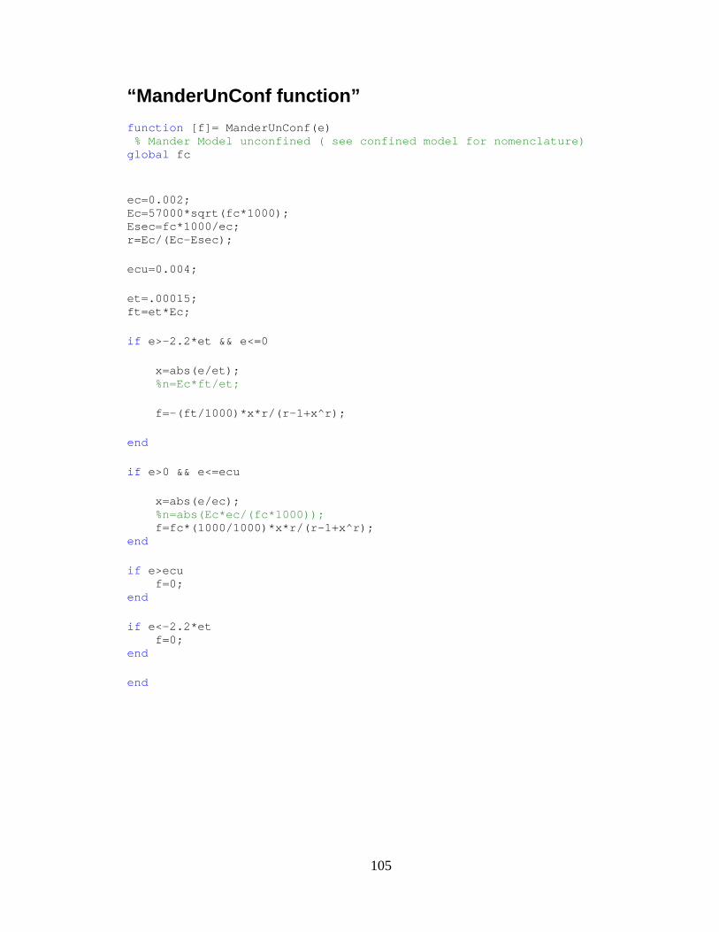
105

“ManderUnConf function”

function [f]= ManderUnConf(e) % Mander Model unconfined ( see confined model for nomenclature) global fc ec=0.002; Ec=57000*sqrt(fc*1000); Esec=fc*1000/ec; r=Ec/(Ec-Esec); ecu=0.004; et=.00015; ft=et*Ec; if e>-2.2*et && e<=0 x=abs(e/et); %n=Ec*ft/et; f=-(ft/1000)*x*r/(r-1+x^r); end if e>0 && e<=ecu x=abs(e/ec); %n=abs(Ec*ec/(fc*1000)); f=fc*(1000/1000)*x*r/(r-1+x^r); end if e>ecu f=0; end if e<-2.2*et f=0; end end

106

“steel function”

function [f]=steel(e) % Steel Stress Function global fy Es esh fu eu Esh ey=fy/Es; if abs(e)<=ey f=abs(e)*Es*sign(e); %Between Yield in Tension & Compression end if abs(e)<=esh && abs(e)>ey f=sign(e)*fy; % More than yield, but before esh in Tension and Compression end if abs(e)>esh && abs(e)<=eu p=Esh*(eu-esh)/(fu-fy); f=(fu+(fy-fu)*(abs((eu-abs(e)))/(eu-esh))^p)*sign(e); % More than esh in Tension and Compression end if abs(e)>eu f=0; % Greater than ultimate in Tension and Compression end end

107

“strain function” function [st1, st2, st3, st4, st5, st6]=strain(curv, na) %-------------- Find Strains in fibers throughout section-------------- global DIVCC DIVCT DIVCB inc Numinc TB BB SB Rowside Height DIVTB SZTB DIVBB SZBB Strain %display(curv); st=curv*(Height/2-na); %display(st); for i=1:inc+1 % Top layer Cover if DIVCT(i,1)>na % Greater than Neutral Axis st1(i,1)=st/(Height/2-na)*(DIVCT(i,1)-na); end if DIVCT(i,1)<na % Less than Neutral axis st1(i,1)=-st/(Height/2-na)*abs(DIVCT(i,1)-na); end if DIVCT(i,1)== na % Neutral Axis st1(i,1)=0; end end for i=1:inc+1 % Bottom Layer Cover if DIVCB(i,1)>na st2(i,1)=st/(Height/2-na)*(DIVCB(i,1)-na); end if DIVCB(i,1)<na st2(i,1)=-st/(Height/2-na)*abs(DIVCB(i,1)-na); end if DIVCB(i,1)== na st2(i,1)=0; end end for i=1:Numinc+1 % Confined Concrete if DIVCC(i,1)>na st3(i,1)=st/(Height/2-na)*(DIVCC(i,1)-na); end if DIVCC(i,1)<na st3(i,1)=-st/(Height/2-na)*abs(DIVCC(i,1)-na); end if DIVCC(i,1)== na st3(i,1)=0; end end

108

for i=1:Numinc+1 % Top Bars if DIVTB(i,1)>na && DIVTB(i,1)>=(TB(1,2)-SZTB/16) && DIVTB(i,1)<=(TB(1,2)+SZTB/16) st4(i,1)=st/(Height/2-na)*(DIVTB(i,1)-na); end if DIVTB(i,1)<na && DIVTB(i,1)>=(TB(1,2)-SZTB/16) && DIVTB(i,1)<=(TB(1,2)+SZTB/16) st4(i,1)=-st/(Height/2-na)*abs(DIVTB(i,1)-na); end if DIVTB(i,1)== na st4(i,1)=0; end if DIVTB(i,1)<(TB(1,2)-SZTB/16) || DIVTB(i,1)>(TB(1,2)+SZTB/16) st4(i,1)=0; end end for i=1:Numinc+1 % Bottom Bars if DIVBB(i,1)>na && DIVBB(i,1)>=(BB(1,2)-SZBB/16) && DIVBB(i,1)<=(BB(1,2)+SZBB/16) st5(i,1)=st/(Height/2-na)*(DIVBB(i,1)-na); end if DIVBB(i,1)<na && DIVBB(i,1)>=(BB(1,2)-SZBB/16) && DIVBB(i,1)<=(BB(1,2)+SZBB/16) st5(i,1)=-st/(Height/2-na)*abs(DIVBB(i,1)-na); end if DIVBB(i,1)== na st5(i,1)=0; end if DIVBB(i,1)<(BB(1,2)-SZBB/16) || DIVBB(i,1)>(BB(1,2)+SZBB/16) st5(i,1)=0; end end if Rowside~=0 % Side Bars for i=1:Rowside if SB(i,3)>na st6=st/(Height/2-na)*(SB(i,3)-na); end if SB(i,3)<na st6=-st/(Height/2-na)*abs(SB(i,3)-na); end if SB(i,3)== na st6=0; end end else st6=0; end

109

Strain=min(st5(:,1)); % Max Tensile Strain for Rectangular section end

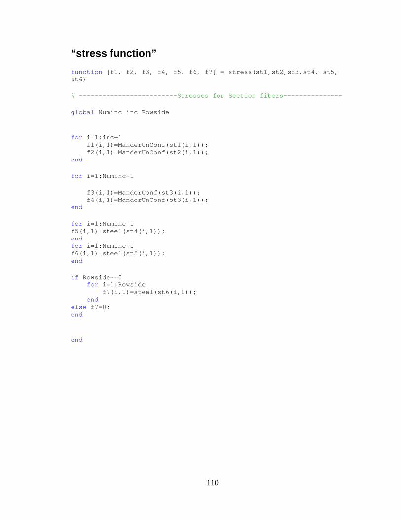
110

“stress function” function [f1, f2, f3, f4, f5, f6, f7] = stress(st1,st2,st3,st4, st5, st6) % -------------------------Stresses for Section fibers--------------- global Numinc inc Rowside for i=1:inc+1 f1(i,1)=ManderUnConf(st1(i,1)); f2(i,1)=ManderUnConf(st2(i,1)); end for i=1:Numinc+1 f3(i,1)=ManderConf(st3(i,1)); f4(i,1)=ManderUnConf(st3(i,1)); end for i=1:Numinc+1 f5(i,1)=steel(st4(i,1)); end for i=1:Numinc+1 f6(i,1)=steel(st5(i,1)); end if Rowside~=0 for i=1:Rowside f7(i,1)=steel(st6(i,1)); end else f7=0; end end