Graphical Tools for Linear Structural Equation …ftp.cs.ucla.edu/pub/stat_ser/r432.pdfGraphical...

Graphical Tools for Linear Structural Equation Modeling

Bryant Chen and Judea PearlUniversity of California, Los Angeles

Computer Science DepartmentLos Angeles, CA, 90095-1596, USA

(310) 825-3243

This paper surveys graphical tools developed in the past three decades that are applicable tolinear structural equation models (SEMs). These tools permit researchers to answer key re-search questions by simple path-tracing rules, even for highly complex models. They includeparameter identification, causal effect identification, regressor selection, selecting instrumentalvariables, finding testable implications of a given model, identifying equivalent models andestimating counterfactual relationships.

Keywords: causal effects, counterfactuals, equivalent models, goodness of fit, graphicalmodels, identification, linear regression, misspecification test

Introduction

Structural Equation Models (SEMs) are the dominant re-search paradigm in the quantitative, data-intensive behav-ioral sciences. These models permit a researcher to expresstheoretical assumptions meaningfully, using equations, de-rive their consequences and test their statistical implicationsagainst data. The result is a powerful symbiosis betweentheory and data which underlies much of current researchin causal analysis, especially in therapy evaluation (Shroutet al., 2010), education testing and management (Muthén andMuthén, 2010), and personality research (Lee, 2012).

While advances in graphical models have had a transfor-mative impact on causal analysis and machine learning, onlya meager portion of these developments have found their wayto mainstream SEM literature which, by and large, prefersalgebraic over graphical representations (Joreskog and Sor-bom, 1982; Bollen, 1989; Mulaik, 2009; Hoyle, 2012). Oneof the reasons for this disparity rests on the fact that graph-ical techniques were developed for non-parametric analysis,while much of SEM research is conducted within the con-fines of Gaussian linear models, to which matrix algebra andpowerful statistical tests are applicable. Among the tasksfacilitated by graphical models are: model testing, identifi-cation, policy analysis, bias control, mediation, external va-lidity, and the analysis of counterfactuals and missing data(Pearl, 2014a).

The purpose of this paper is to introduce psychometricresearchers to modern tools of graphical models and to de-scribe some of the benefits, as well as new insights thatgraphical models can provide. We will begin by introduc-ing basic definitions and tools used in graphical modeling,including graph construction, definitions of causal effects,and Wright’s path tracing rules. We then introduce more ad-

vanced notions of graph separation, which were developedfor non-parametric analysis, but have simple and meaning-ful interpretation in linear models. These tools provide thebasis for model testing and identification criteria, discussedin subsequent sections. We then cover advanced applicationsof path diagrams including equivalent regressor sets, mini-mal regressor sets, and variance minimizing for causal ef-fect estimation. Lastly, we discuss counterfactuals and theircomputation in linear SEMs before showing how the toolspresented in this paper provide simple solutions to five ex-amples representing non-trivial problems in SEM research.

With the exception of the “Causal Effects among LatentVariables" section, we focus on models where all variablesare observable (often called path analysis models), allowingfor error terms to be correlated. As graphical techniqueswere originally developed for non-parametric models, theyhave not traditionally addressed the identification of effectsamong latent variables, which is impossible without para-metric assumptions. Instead, the presence of latent variableswas taken into account through the correlations they induceon the error terms. We will demonstrate how latent variablescan be summarized using error terms and briefly discuss howthe results in this paper, while not directly addressing causaleffects among latent variables, can nevertheless be applied totheir analysis.

Path Diagrams and Graphs

Path diagrams or graphs1 are graphical representations ofthe model structure. They were introduced by Sewell Wright(1921), who aimed to estimate causal influences from sta-tistical data on animal breeding. Today, SEM is generally

1We use both terms interchangeably.

TECHNICAL REPORT R-432

July 2015

2 BRYANT CHEN AND JUDEA PEARL

implemented in software2, and, as a result, when users expe-rience unexpected behavior (due to unidentified parameters,for example) they are often at a loss as to the source of theproblem3. For the remainder of this section, we will reviewthe basics of path diagrams and provide users with simple,intuitive tools that will be used to resolve questions of identi-fication, goodness of fit, and more using graphical methods.

We introduce path diagrams by way of example. Supposewe wish to estimate the effect of attending an elite collegeon future earnings. Clearly, simply regressing earnings oncollege rating will not give an unbiased estimate of the targeteffect. This is because elite colleges are highly selective, sostudents attending them are likely to have qualifications forhigh-earning jobs prior to attending the school. This back-ground knowledge can be expressed in the following SEMspecification. Throughout the paper, we will use lowercaseletters and the Greek letter α to represent model parameters.

Model 1.

Q1 = U1

C = a · Q1 + U2

Q2 = c ·C + d · Q1 + U3

S = b ·C + e · Q2 + U4,

where Q1 represents the individual’s qualifications prior tocollege, Q2 represents qualifications after college, C containsattributes representing the quality of the college attended,and S the individual’s salary.

Figure 1a is a causal graph that represents this model spec-ification. Each variable in the model has a correspondingnode or vertex in the graph. Additionally, for each equa-tion, arrows are drawn from the independent variables to the

(a)

(b)

Figure 1. (a) Model with latent variables (Q1 and Q2) shownexplicitly (b) Same model with latent variables summarized

dependent variables. These arrows reflect the direction ofcausation. In some cases, we may label the arrow with itscorresponding structural coefficient as in Figure 1a. Errorterms are typically not displayed in the graph, unless theyare correlated.

The variables Q1 and Q2 represent quantities that are notdirectly measurable. As a result, they are latent variables.In this paper, we distinguish latent variables from observ-able variables in the graph by surrounding the former with adashed box. As we mentioned in the Introduction, the pres-ence of latent variables is taken into account by the corre-lations they induce on the error terms4. For example, theeffect of the latent variables in Figures 1a is summarized byFigure 1b. We see that the effect of College on Salary inFigure 1a is now summarized by the coefficient α in Figure1b. Similarly, the bidirected arc between C and S (represent-ing the correlation of the error terms of C and S ) in Figure1b summarizes the correlation between C and S due to thepath C ← Q1 → Q2 → S . The corresponding model is asfollows:

Model 2.

C = UC

S = αC + US

The background information specified by Model 1 impliesthat the error term of S , US , is not correlated with UC , andthis correlation is depicted in Figure 1a by the bidirected arcbetween C and S .

In order to estimate α, the causal effect of attending anelite college on future earnings, the coefficients must have aunique solution in terms of the covariance matrix or probabil-ity distribution over the observable variables, C and S . Thetask of finding this solution is known as identification and isdiscussed in a later section. In some cases, one or more co-efficients may not be identifiable, meaning that no matter thesize of the dataset, it is impossible to obtain point estimatesfor their values. Indeed, we will see that the coefficients inModel 1 are not identified if Q1 and Q2 are latent. However,if we include the strength of an individual’s college appli-cation, A, as shown in Figure 2a, we obtain the followingmodel:

2Common software packages include AMOS (Arbuckle, 2005),EQS (Bentler, 1989), LISREL (Jöreskog and Sörbom, 1989), andMPlus (Muthén and Muthén, 2010) among others.

3Kenny and Milan (2012) write, “Identification is perhaps themost difficult concept for SEM researchers to understand. We haveseen SEM experts baffled and bewildered by issues of identifica-tion.”

4While we do not directly address the identification of causaleffects among latent variables, the results in this paper are neverthe-less applicable to this problem. See section Identification.

GRAPHICAL TOOLS FOR LINEAR STRUCTURAL EQUATION MODELING 3

(a)

(b)

Figure 2. Graphs associated with Model 3 in the text (a)with latent variables shown explicitly (b) with latent vari-ables summarized

Model 3.

Q1 = U1

A = a · Q1 + U2

C = b · A + U3

Q2 = e · Q1 + d ·C + U4

S = c ·C + f · Q2 + U5.

By removing the latent variables from the model specifica-tion we obtain:

Model 4.

A = a · Q1 + UA

C = b · A + UC

S = α ·C + US .

The corresponding path diagram is displayed in Figure2b. The coefficients in this model are combinations of coef-ficients of the original model and each of these combinationsis identifiable, as we will show.

The ability to determine identifiability directly from themodel specification is a valuable feature of graphical mod-els. For example, it would be a waste of resources to specifythe structure in Model 2 and gather data only to find that theparameter of interest is not identified. The tools provided insubsequent sections will allow modelers to determine imme-diately from the path diagram that the effect of attending anelite college on future salary, α, is not identified using Model2 but is identified (and equal to the coefficient of C in theregression of S on C and A, denoted βS C.A) using Model 4.This conclusion is a consequence of the model specification

and α = βS C.A holds only if the specification accurately re-flects reality (see section “Causal Effects among Latent Vari-ables"). The ability to derive testable implications and testthe model specification is another valuable feature of graph-ical models. For example, we will see that Model 3 impliesthat the partial correlation between S and A given C and Q1,ρS A.CQ1 , is equal to zero. If this constraint does not hold inthe data, then we have evidence that the model is missing ei-ther an arrow or a bidirected arc between A and S . Most im-portantly, these tools will be applicable to far more complexmodels where questions of identifiability and testable impli-cations are near impossible to determine by hand or even bystandard software.

In summary, the causal graph is constructed from themodel equations in the following way: Each variable in themodel has a corresponding vertex or node in the graph. Foreach equation, arrows are drawn in the graph from the nodesrepresenting dependent variables to the node representing theindependent variable. Each arrow, therefore, is associatedwith a coefficient in the SEM, which we will call its struc-tural coefficient. Finally, if the error terms of any two vari-ables are correlated, then a bidirected arc is drawn betweenthe two variables. Conversely, the lack of a bidirected arcindicates that the error terms are independent.

Before continuing, we review some basic graph terminol-ogy. An edge is defined to be either an arrow or a bidirectedarc. If an arrow exists from X to Y , we say that X is a parentof Y . If there exists a sequence of arrows all of which aredirected from X to Y we say that X is an ancestor of Y . If Xis an ancestor of Y then Y is a descendant of X. Finally, theset of nodes connected to Y by a bidirected arc are called thesiblings of Y .

A path between X and Y is a sequence of edges, connect-ing the two vertices5. A path may go either along or againstthe direction of the arrows. A directed path from X to Y isa path consisting only of arrows pointed towards Y . A back-door path from X to Y is a path begins with an arrow pointingto X and ends with an arrow pointing to Y . For example, inFigure 4, C ← B→ E, C → D→ E, C ← B→ D→ E, andC → D ← B → E are all paths between C and E. However,only C → D → E is a directed path, and only C ← D → Eand C ← B→ D→ E are back-door paths. The significanceof directed paths stems from the fact that they convey theflow of causality, while the significance of back-door pathsstems from their association with confounding.

A node in which two arrowheads meet is called a collider.For example, Z in Figure 5a and C in Figure 4 are colliders.The significance of colliders stems from the fact that theyblock the flow of information along a path (see section D-separation).

A graph or model is acyclic if it does not contain any cy-

5We emphasize that, in this paper, we refer to paths as sequencesof arrows and/or bidirected arcs, not single arrows.


cles, that is a directed path that begins and ends with thesame node. A model or graph is cyclic if it contains a cy-cle. An acyclic model without correlated error terms is calledMarkovian. Models with correlated error terms are callednon-Markovian while acyclic non-Markovian models are ad-ditionally called semi-Markovian. For example, Figure 4 isboth acyclic and Markovian. If we were to add a bidirectedarc between any two variables, then it would no longer beMarkovian and would instead be semi-Markovian. If wewere to instead reverse the edge from B to E, then we wouldcreate a cycle and the model would be non-Markovian andcyclic.

Lastly, we note that, for simplicity, we will assume with-out loss of generality that all variables have been standard-ized to mean 0 and variance 1.

Causal Effects

Let Π = {π1, π2, ..., πk} be the set of directed paths from Xto Y and pi be the product of the structural coefficients alongpath πi. The total effect or average causal effect (ACE) of Xon Y is often defined as the

∑i pi (Bollen, 1989). For exam-

ple, in Figure 2a, the total effect of C on S is c+d · f and thatof A on S is b(c + d f ).

The rational for this additive formula and its extension tonon-linear systems can best be seen if we define the causaleffect of X on Y as the expected change in Y when X is as-signed to different values by intervention, as in a randomizedexperiment. The act of assigning a variable X to the valuex is represented by removing the structural equation for Xand replacing it with the equality X = x. This replacementdislodges X from its prior causes and ensures that covariationbetween X and Y reflects causal paths from X to Y only.

The expected value of a variable, Y , after X is assigned thevalue x by intervention is denoted E[Y |do(X = x)], and theACE of X on Y is defined as

ACE = E[Y |do(X = x + 1)] − E[Y |do(X = x)], (1)

where x is some reference point (Pearl, 2009, ch. 5)6. In non-linear systems, the effect will depend on the reference pointbut in the linear case, x will play no role and we can replace(1), with the derivative,

ACE =∂

∂xE[Y |do(X = x)]. (2)

Consider again Model 3 with C a binary variable takingvalue 1 for elite colleges and 0 for non-elite colleges. To es-timate the total effect of attending an elite college on salary,we would hypothetically assign each member of the pop-ulation to an elite college and observe the average salary,E[S |do(C = 1)]. Then we would rewind time and assigneach member to a non-elite college, observing the new aver-age salary, E[S |do(C = 0)]. Intuitively, the causal effect of

attending an elite college is the difference in average salary,

E[S |do(C = 1)] − E[S |do(C = 0)].

The above operation provides a mathematical procedure thatmimics this hypothetical (and impossible) experiment usinga SEM.

In linear systems, this “interventional” definition of causaleffect coincides with the aforementioned “path-tracing” def-inition as we will demonstrate by computing E[S |do(C =

1)] − E[S |do(C = 0)] in Model 3. (For clarity, we will con-sider Q1 and Q2 to be observable and not latent variables forthe remainder of this section.)

The intervention, do(C = c0), modifies the equations inthe following way:

Model 5.

Q1 = U1

A = a · Q1 + U2

C = c0

Q2 = e · Q1 + d ·C + U4

S = c ·C + f · Q2 + U5.

The corresponding path diagram is displayed in Figure 3a.Notice that back-door paths, due to common causes, betweenC and S have been cut, and as a result, all unblocked pathsbetween C and S now reflect the causal effect of C on S only.

Recalling that we assume model variables have been stan-dardized to mean 0 and variance 1 implying that E[Ui] = 0for all i, we see that setting C to c0 gives the following ex-pectation for S :

E[S |do(C = c0)] = E[c ·C + f · Q2 + U5]= c · E[C] + f · E[Q2] + E[U5]= c · c0 + f E[e · Q1 + d ·C + U4]= c · c0 + f · e · E[U1] + f · d · c0 + f · E[U4]= c · c0 + f · d · c0

As a result,

E[S |do(C = c0 + 1)] − E[S |do(C = c0)] = c + f d (3)

for all c0, aligning the two definitions7.6Holland (2001) defines causal effects in counterfactual termi-

nology (also known as potential outcomes (Rubin, 1974)), whichwill be discussed in section Counterfactuals in Linear Models. Thelogical equivalence between these two notational systems is shownin (Pearl, 2009, ch. 7.4). SEMs provide a semantics for the poten-tial outcomes framework, which is based on scientific knowledge asopposed to experimental design.

7Moreover, this equality holds even when the parameters, c, d,and f , are not identified (e.g. if the U terms are correlated). Causaleffects are defined in terms of hypothetical interventions, and theparameters determine the impact of these interventions. Identifica-tion is only the means to obtain causal effects from statistical dataand has nothing to do with the definition.


In many cases, we may be interested in the direct effect ofC on S . The term “direct effect” is meant to quantify an effectthat is not mediated by other variables in the model or, moreaccurately, the sensitivity of S to changes in C while all otherfactors in the analysis are held fixed (Pearl, 2009, ch. 4.5).In Model 3, the direct effect of C on S represents the effectson salary due to factors other than the superior qualificationsobtained by attending an elite college. For example, it couldrepresent the value that employers place on the reputation ofthe school.

“Holding all other factors fixed” can be simulated by inter-vening on all variables other than C and S and assigning theman arbitrary set of reference values8. (Like the total effect, inlinear systems, the direct effect does not change with respectto the reference values.) Doing so severs all causal links inthe model other than those leading into S . As a result, alllinks from C to S other than the direct link will be severed.For example, Figure 3b shows the path diagram of Model 3after intervention on all variables other than C and S .

Now, the direct effect of C on S can be defined as

E[S |do(C = c0 + 1,T = t)] − E[S |do(C = c0,T = t)],

where T is a set containing all model variables other than Cand S and {c0 ∪ t} a set of reference values. This causallydefined notion of direct effect differs fundamentally from thetraditional definition which is based on conditioning on in-termediate variables (Baron and Kenny, 1986). The formeris valid in the presence of correlated errors and permits us toextend this notion to non-linear models (Pearl, 2014b).

Notice that the direct effect of C on S in Figure 2b is equalto the total effect of C on S in Figure 2a. Direct effects de-pend on the set of variables that we decide to include in themodel.

Lastly, in linear models, the effect of C on S mediated byQ2 is equal to the sum of the product of coefficients associ-ated with directed paths from C to S that go through Q2 (i.e.the effect on salary due to the knowledge and skills obtainedfrom attending an elite college). In Figure 2a, we see that thiseffect is equal to d f . For a non-linear and non-parametric ex-tension of this definition, see indirect effect in (Pearl, 2014b).

Wright’s Path Tracing Rules

The earliest usage of graphs in causal analysis can befound in Sewell Wright’s 1921 paper, “Correlation and Cau-sation”. This seminal paper gives a method by which thecovariance of any two variables in an acyclic, standardizedmodel can be expressed as a polynomial over a subset of themodel coefficients.

Wright’s method consists of equating the covariance, σYX ,between any pair of variables, X and Y , to the sum of prod-ucts of structural coefficients and error covariances along cer-tain paths between X and Y . Let Π = {π1, π2, ..., πk} denotethe paths between X and Y that do not trace a collider, and

(a)

(b)

Figure 3. Models depicting interventions (a) After interven-ing on C (c) After intervening on C, A, Q1, and Q2

let pi be the product of structural coefficients along path πi.Then the covariance between variables X and Y is

∑i pi. For

example, we can calculate the covariance between C and Sin Figure 2b in the following way: First, we note that thereare two paths between C and S and neither trace a collider,π1 = C → S and π2 = C ← A ↔ S . The product of thecoefficients along these paths are p1 = α and p2 = b · CAS .Summing these products together we obtain the covariancebetween C and S , σCS = α + b ·CAS .

Consider the more complicated example of calculatingσCE in Figure 4. The paths between C and E that do nottrace a collider are C ← F → A → E, C ← A → E, andC → D → E. (Note that we do not include C → D ← B →E because it traces a collider, D.) Summing the products ofcoefficients along these paths gives σCE = b ·a ·g+c ·g+d ·h.

To express the partial covariance, σYX.Z , partial correla-tion, ρYX.Z or regression coefficient, βYX.Z , of Y on X given Z

8In footnote 15 we give an example demonstrating that “holdingall other factors fixed” cannot be simulated using conditioning butinstead must invoke intervention.

Figure 4. Model illustrating Wright’s path tracing rules andd-separation


in terms of structural coefficients we can first apply the fol-lowing reductions given by Crámer (1946), before utilizingWright’s rules. When Z is a singleton, these reductions are:

ρYX.Z =ρYX − ρYZρXZ

[(1 − ρ2YZ)(1 − ρ2

XZ)]12

(4)

σYX.Z = σYX −σYZσZX

σ2Z

(5)

βYX.Z =σY

σX

ρYX − ρYZρZX

1 − ρ2XZ

(6)

When Z is a singleton and S a set, we can reduce ρYX.ZS ,σYX.ZS , or βYX.ZS as follows:

ρYX.ZS =ρYX.S − ρYZ.S ρXZ.S

[(1 − ρ2YZ.S )(1 − ρ2

XZ.S )]12

(7)

σYX.ZS = σYX.S −σYZ.SσZX.S

σ2Z.S

(8)

βYX.ZS =σY.S

σX.S

ρYX.S − ρYZ.S ρZX.S

1 − ρ2XZ.S

(9)

We see that ρYX.ZS , σYX.ZS , or βYX.ZS can be expressed interms of pair-wise coefficients by recursively applying theabove formulas for each element of S . Then, using Equations4-9, we can express the reduced pairwise covariances / cor-relations in terms of the structural coefficients. For example,reducing βCS .A for Figure 2b can be done as follows:

βCS .A =σC

σS

ρCS − ρCAρAS

1 − ρ2S A

(10)

=11

(α + bCAS ) − (bα + CAS )(b)1 − b2 (11)

=α + bCAS − b2α − bCAS

1 − b2 (12)

=α − b2α

1 − b2 (13)

= α (14)

D-Separation

When the conditioning set becomes large, applying the re-cursive formula of Equations 7-9 can become complex. Van-ishing partial correlations, however, can be readily identifiedfrom the path diagram using a criterion called d-separation(Pearl, 1988)9. In other words, d-separation allows us todetermine whether correlated variables become uncorrelatedwhen conditioning on a given set of variables. Not only willthis criterion allow us to use these zero partial correlationsfor model testing, but it will also be utilized extensively inthe analysis of identification that follows.

The idea of d-separation is to associate “correlation”with “connectedness” in the graph, and independence with

(a)

(b)

Figure 5. Examples illustrating conditioning on a collider

“separation”. The only twist on this simple idea is to definewhat we mean by “connected path”, since we are dealingwith a system of directed arrows in which some nodes (thoseresiding in the conditioning set, Z) correspond to variableswhose values are given. To account for the orientations of thearrows we use the terms “d-separated” and “d-connected” (ddenotes “directional”).

Rule 1: X and Y are d-separated if there is no active pathbetween them.

By “active path”, we mean a path that can be traced with-out traversing a collider. If no active path exists betweenX and Y then we say that X and Y are d-separated. As wecan see from Wright’s rules, ρXY = 0 when X and Y are d-separated.

When we measure a set Z of variables, and take theirvalues as given, the partial covariances of the remainingvariables changes character; some correlated variablesbecome uncorrelated, and some uncorrelated variablesbecome correlated. To represent this dynamic in the graph,we need the notion of “partial d-connectedness” or moreconcretely, “d-connectedness conditioned on a set Z ofmeasurements”.

Rule 2: X and Y are d-connected, conditioned on a set of Znodes, if there is a collider-free path between X and Y thattraverses no member of Z. If no such path exists, we saythat X and Y are d-separated by Z or we say that every pathbetween X and Y is “blocked” by Z.

A common example used to show that correlation does notimply causation is the fact that ice cream sales are correlatedwith drowning deaths. When the weather gets warm people

9See also Hayduk et al. (2003) and Mulaik (2009) for an intro-duction to d-separation tailored to SEM practitioners.


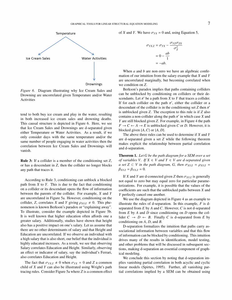
Figure 6. Diagram illustrating why Ice Cream Sales andDrowning are uncorrelated given Temperature and/or WaterActivities

tend to both buy ice cream and play in the water, resultingin both increased ice cream sales and drowning deaths.This causal structure is depicted in Figure 6. Here, we seethat Ice Cream Sales and Drownings are d-separated giveneither Temperature or Water Activities. As a result, if weonly consider days with the same temperature and/or thesame number of people engaging in water activities then thecorrelation between Ice Cream Sales and Drownings willvanish.

Rule 3: If a collider is a member of the conditioning set Z,or has a descendant in Z, then the collider no longer blocksany path that traces it.

According to Rule 3, conditioning can unblock a blockedpath from X to Y . This is due to the fact that conditioningon a collider or its descendant opens the flow of informationbetween the parents of the collider. For example, X and Yare uncorrelated in Figure 5a. However, conditioning on thecollider, Z, correlates X and Y giving ρXY.Z , 0. This phe-nomenon is known Berkson’s paradox or “explaining away”.To illustrate, consider the example depicted in Figure 5b.It is well known that higher education often affords one agreater salary. Additionally, studies have shown that heightalso has a positive impact on one’s salary. Let us assume thatthere are no other determinants of salary and that Height andEducation are uncorrelated. If we observe an individual witha high salary that is also short, our belief that the individual ishighly educated increases. As a result, we see that observingSalary correlates Education and Height. Similarly, observingan effect or indicator of salary, say the individual’s Ferrari,also correlates Education and Height.

The fact that σYX.Z , 0 when σYX = 0 and Z a commonchild of X and Y can also be illustrated using Wright’s pathtracing rules. Consider Figure 5a where Z is a common effect

of X and Y . We have σYX = 0 and, using Equation 5,

σYX.Z = σYX −σYZσZX

σ2Z

= 0 −ab1

= −ab.

When a and b are non-zero we have an algebraic confir-mation of our intuition from the salary example that X and Yare uncorrelated marginally, but becoming correlated whenwe condition on Z.

Berkson’s paradox implies that paths containing colliderscan be unblocked by conditioning on colliders or their de-scendants. Let π′ be a path from X to Y that traces a collider.If for each collider on the path π′, either the collider or adescendant of the collider is in the conditioning set Z then π′

is unblocked given Z. The exception to this rule is if Z alsocontains a non-collider along the path π′ in which case X andY are still blocked given Z. For example, in Figure 4 the pathF → C ← A→ E is unblocked given C or D. However, it isblocked given {A,C} or {A,D}.

The above three rules can be used to determine if X and Yare d-separated given a set Z while the following theoremmakes explicit the relationship between partial correlationand d-separation.

Theorem 1. Let G be the path diagram for a SEM over a setof variables V. If X ∈ V and Y ∈ V are d-separated givena set Z ⊂ V in the path diagram, G, then σXY.Z = ρXY.Z =

βXY.Z = βYX.Z = 0.

If X and Y are d-connected given Z then σXY.Z is generallynot equal to zero but may equal zero for particular parame-terizations. For example, it is possible that the values of thecoefficients are such that the unblocked paths between X andY perfectly cancel one another.

We use the diagram depicted in Figure 4 as an example toillustrate the rules of d-separation. In this example, F is d-separated from E by A and C. However, C is not d-separatedfrom E by A and D since conditioning on D opens the col-lider C → D ← B. Finally C is d-separated from E byconditioning on A, D, and B.

D-separation formalizes the intuition that paths carry as-sociational information between variables and that this flowof information can be blocked by conditioning. This intuitiondrives many of the results in identification, model testing,and other problems that will be discussed in subsequent sec-tions, making d-separation an essential component of graph-ical modeling.

We conclude this section by noting that d-separation im-plies vanishing partial correlation in both acyclic and cycliclinear models (Spirtes, 1995). Further, all vanishing par-tial correlations implied by a SEM can be obtained using


d-separation (Pearl, 2009, ch. 1.2.3). Finally, in modelswith independent error terms, these vanishing partial correla-tions represent all of the model’s testable implications (Pearl,2009, ch. 5.2.3).

Identification

A model parameter is identified if it can be uniquely deter-mined from the probability distribution over the model vari-ables. If a parameter is not identified, then it cannot be esti-mated from data because there are many (often infinite) val-ues for the parameter compatible with a given dataset.

If every parameter in the model is identified then themodel is said to be identified. If there is at least one uniden-tified parameter than the model is not identified or unidenti-fied10.

In SEMs, a parameter can be identified by expressing ituniquely in terms of the covariance matrix. For example,consider the model represented by Figure 2b. In the previ-ous section (see Equations 10-14), we used Wright’s rulesto show that the parameter α, which is equivalent to thecausal effect of C on S , is identified and equal to βS C.A =σ2

AσCS−σCAσAS

σ2Sσ

2A−σ

2S A

.In contrast, α is not identified in Figure 1b, whose stan-

dardized covariance matrix is:(1 σS C

σS C 1

)Using Wright’s rules we obtain a single equation: α+ CCS =

σS C . Since there are infinite values for α and CCS that satisfythis equation, neither parameter is identified and the model isnot identified11.

Many SEM researchers determine the identifiability of themodel by submitting the specification and data to software,which attempts to estimate the coefficients by minimizing afitting function12. If the model is not identified, then the pro-gram will be unable to complete the estimation and warnsthat the model may not be identified. While convenient,there are disadvantages to using typical SEM software to de-termine model identifiability (Kenny and Milan, 2012). Ifpoor starting values are chosen, the program could mistak-enly conclude the model is not identified when in fact it maybe identified. When the model is not identified, the programis not helpful in indicating which parameters are not iden-tified nor are they able to provide estimates for identifiablecoefficients13. Most importantly, the program only gives ananswer after the researcher has taken the time to collect data.

Rather than determining the identifiability of parametersby fitting the model, the tools described in this paper enableus to detect identifiability directly from the model specifica-tion and express identified parameters in terms of the popu-lation covariance matrix. As a result, the modeler can esti-mate their values from the sample covariance matrix, usually

invoking only a few variables, and the resulting estimateswill be consistent, as long as the model accurately reflectsthe data generating mechanism. (In the next section, ModelTesting, we will give graphical criteria for testing whetherthis is indeed the case.) Futher, we avoid issues of poor start-ing values, are able to identify individual parameters whenthe model as a whole is not identified, and can determinethe identifiability of parameters prior to collecting data. Forexample, in the previous section, we demonstrated, withoutdata, that αwas not identified in Figure 1b, but was identifiedin Figure 2b. As a result, the researcher knows when design-ing the study that if α is the effect of interest, she must collectdata on A, in addition to C and S .

In this section, we give graphical criteria that allow themodeler to determine whether a given parameter is identifiedby inspecting the path diagram. While these methods are notcomplete in the sense that they may not be able to identifyevery coefficient that is identifiable, they subsume the identi-fiability rules in the existing SEM literature, including the re-cursive and null rules (Bollen, 1989) and the regression rule(Kenny and Milan, 2012).

Selecting Regressors

It is well known that the coefficients of a structural equa-tion, Y = α1X1 + α2X2 + ... + αkXk + UY , are identified andcan be estimated using regression if the error term, U, is in-dependent of X = {X1, X2, ...Xk}. However, in some cases,αi can be estimated using regression even when X is corre-lated with U. For example, we showed that α in Figure 2bis equal to βCS .A (see Equations 10-14), even though in thecorresponding structural equation, S = αC + US , permits Cand US to be correlated. As a result, α can be estimated usingthe regression S = β1C + β2A + εS , which yields α = β1

14.

10Many authors also use the term “under-identified”. This termcan be confusing because it suggests models that are not identifiablehave no testable implications. This is not the case.

11While α is is not identified in Figure 1b, the causal effect ofC on S is still well-defined. It is equal to E[S |do(C = 1)] −E[S |do(C = 0)] = α. The fact that this quantity is not identifiedsimply means that we cannot estimate it from data on C and S alone.

12Determining identifiability by fitting a model has become socommonplace in the SEM community that it is often forgotten thatidentification and model testing are separate concepts. Identifia-bility is a property of the model specification only, and remainsindependent of the data actually observed. “Fitting", on the otherhand, is a relationship between the model specification and the dataobserved. Models can be “fitted" or “tested for fitting" regardless ofwhether they are identified, although most available software todayrequire identification for “fitting" to produce meaningful results.

13According to Kenny and Milan (2012), AMOS is the only pro-gram that attempts to estimate parameters when the model is notidentified.

14We distinguish between structural equations, in which theparameters, α1, α2, ..., αk, represent causal effects, and regression


Adding a set of variables, Z, to a regression to estimatea parameter is often called adjusting for Z. The questionarises, how can we, in general, determine whether a set ofvariables is adequate for adjustment when attempting to iden-tify a given structural coefficient α? Put another way, howcan we determine whether a set Z of variables, when addedto the regression of Y on X would render the slope (of Y on X)equal to the desired structural coefficient, α? The followingcriterion, called single-door, allows the modeler to answerthis question by inspection of the path diagram.

Theorem 2. (Pearl, 2009, ch. 5.3.1) (Single-door Criterion)Let G be any acyclic causal graph in which α is the coeffi-cient associated with arrow X → Y, and let Gα denote thediagram that results when X → Y is deleted from G. Thecoefficient α is identifiable if there exists a set of variablesZ such that (i) Z contains no descendant of Y and (ii) Z d-separates X from Y in Gα. If Z satisfies these two conditions,then α is equal to the regression coefficient βYX.Z . Conversely,if Z does not satisfy these conditions, then βYX.Z is not a con-sistent estimand of α (except in rare instances of measurezero).

In Figure 7a, we see that W blocks the spurious pathX ← Z → W → Y and X is d-separated from Y by W inFigure 7b. Therefore, α is identified and equal to βYX.W . Thisis to be expected since X is independent of UY in the struc-tural equation, Y = αX + cW + UY . Theorem 2 tells us,however, that Z can also be used for adjustment since Z alsod-separates X from Y in Figure 7b, and we obtain α = βYX.W .(We will see in a subsequent section, however, that the choiceof W is superior to that of Z in terms of estimation power.)

(a) (b)

(c)

Figure 7. Diagrams illustrating identification by the single-door criterion (a) α is identified by adjusting for Z or W (b)The graph Gα used in the identification of α (c) α is identifiedby adjusting for Z (or Z and W) but not W alone

Consider, however, Figure 7c. Z satisfies the single-door cri-terion but W does not. Being a collider, W unblocks the spu-rious path, X ← Z → W ↔ Y , in violation of Theorem 2,leading to bias if adjusted for15. In conclusion, α is equal toβYX.Z in Figures 7a and 7c. However, α is equal to βYX.W inFigure 7a only.

Returning to Figure 2a, we see that S is d-separated fromC given A when we remove the edge from S to C, confirmingthat βS C.A = α.

The intuition for the requirement that Z not be a descen-dant of Y is depicted in Figures 8a and 8b. We typically donot display the error terms, which can be understood as latentcauses. In Figure 8b, we show the error terms explicitly. Itshould now be clear that Y is a collider and conditioning on Zwill create spurious correlation between X, UY , and Y leadingto bias if adjusted for. This means that α can be estimated bythe regression slope of Y on X, but adding Z to the regressionequation would distort this slope, and yield a biased result.

Notice that any coefficient, say from X to Y , is identifiablein a Markovian model using the single-door criterion, sincePa(Y) \ {X} is a single-door admissible set. As a result, thestructural equation for Y , which consists of X and the otherparents of Y , can be converted into a regression equation thatgives an unbiased estimate of each coefficient in the equation.For example, in Figure 4, f is identifiable because the otherparents of E, D and A, represent a single-door admissible

equations, in which the coefficients, β1, β2, ..., βk represent regres-sion slopes. The equation, S = β1C + β2A + εS , is a regres-sion equation, where β1 = ∂

∂C E[S |C, A], β2 = ∂∂A E[S |C, A], and

εS = S − β1C − β2A the residual term. The equation is not structuralsince β2 does not equal the direct effect of A on S , ∂

∂A E[S |do(C, A)],which equals 0. It is for this reason that we refrain from referring toS = β1C + β2A + εS as a regression “model". It is merely a specifi-cation for running a least square routine on the data and estimatingthe slopes β1 and β2.

15 It is for this reason that the direct effect cannot be definedby conditioning on a mediator but must instead invoke intervention(Pearl, 2014b,c), as we did earlier.

(a)

(b)

Figure 8. Example showing that adjusting for a descendantof Y induces bias in the estimation of α


set. The same is true for the other coefficients, g and h. Asa result, each of these coefficients is identified and can beestimated using the regression, E = β1A + β2B + β3D + ε.Using this method, we have the following lemma:

Lemma 1. Any Markovian (acyclic without correlated errorterms) model can be identified equation by equation usingregression.

No matter how complex the model, the single-door theo-rem gives us a quick and reliable criterion for identificationof a structural parameter using regression. It allows us tochoose a variety of regressors using considerations of esti-mation power, sample variability, cost of measurement andmore. Further, it is an important tool that plays a role in theidentification of parameters in more elaborate models.

Instrumental Variables

In Figure 9a, no single-door admissible set exists for αand it cannot be estimated using regression. However, usingWright’s equations we see that σYZ = γα and σXZ = γ. As aresult, α = σYZ

σXZ. In this case, we were able to identify α using

an auxiliary variable Z called an instrumental variable (IV).In this subsection, we will provide a graphical method that

allows modelers to quickly determine whether a given vari-able is an IV by inspecting the path diagram. Additionally,we will introduce conditional instrumental variables and in-strumental sets, which will significantly increase the identi-fication power of the instrumental variable method.

The usage of IVs to identify causal effects in the presenceof confounding can be traced back to Sewall Wright (1925)and his father Philip Wright (1928), and the following is astandard definition adapted from Bollen (2012):

Definition 1. For a structural equation, Y = α1X1 + ... +

αkXk + UY , Zi is an instrumental variable if

(i) Zi is correlated with X = {X1, ..., Xk} and

(ii) Zi is uncorrelated with UY .

Implicit in this definition is that Zi has no effect on Y ex-cept through X. According to Bollen (2012), a necessary

(a) (b)

Figure 9. (a) Z qualifies as an instrumental variable (b) Z isan instrumental variable given W

condition for the identification of α1, ..., αk is that there ex-ists at least k IVs satisfying (i) and (ii), but this condition isnot sufficient.

As is typical in the SEM literature, the above definition de-fines an IV relative to an equation. However, by defining anIV relative to a specific parameter, we will be able to greatlyexpand the power of IVs. First, this will allow the identi-fication of parameters of interest, even when the equation,as a whole, is not identifiable. For example, in Figure 10a,α =

βYZ1βX1Z1

and is identified but γ is not. Second, we refine theconditions under which the equation, as a whole, is identifiedusing IVs. For example, in Figure 10b, we have two instru-ments for Y satisfying the condition of Definition 1, yet (aswe shall see later) γ remains unidentified. A sufficient condi-tion for the identification of an equation with k coefficients isthe existence of at least one IV for each coefficient. Finally,thinking about IVs as pertaining to individual parameters willalso allows us to generalize them and develop new tools likeinstrumental sets.

Economists have always recognized the benefit of defin-ing IVs relative to parameters rather than equations (Wright,1928; Bowden and Turkington, 1984) but have had difficul-ties articulating the conditions that would qualify a variableZ as an instrument in a system of multiple equations. Forexample, the following requirements for an instrument areoffered by Angrist and Pischke (2014):

(i) The instrument has a causal effect on the variablewhose effects we’re trying to capture...

(ii) Z is randomly assigned or “as good as randomly as-signed," in the sense of being unrelated to the omittedvariables that we would like to control for...

(iii) Finally, IV logic requires an exclusion restriction. Theexclusion restriction describes a single channel throughwhich the instrument affects outcomes.

As we shall see from the graphical criterion of Definition 2,condition (i) is overly restrictive; a proxy of an instrumentcould also qualify as an instrument. Condition (ii) leavesambiguous the choice of those “omitted variables", and con-dition (iii) wrongly excludes multiple channels between Zand X, as well as between X and Y .

The following graphical characterization rectifies suchambiguities and allows us to determine through quick in-spection of the path diagram whether a given variable is aninstrument for a given parameter. Moreover, it provides anecessary and sufficient condition for when αi in the equationY = α1X1 + ... + αkXk + UY is identified by βYZi

βXiZi.

Definition 2. (Pearl, 2009, p. 248) A variable Z qualifies asan instrumental variable for coefficient α from X to Y if

(i) Z is d-separated from Y in the subgraph Gα obtainedby removing edge X → Y from G and


(ii) Z is not d-separated from X in Gα.

In Figure 9a, Z is d-separated from Y when we removethe edge associated with α. As a result, Z is an instrumentalvariable for α and we have α =

βYZβXZ

.Now, consider Figure 9b. In this diagram, Z is not an

instrument for α because it is d-connected to Y through thepath Z ← W ↔ Y , even when we remove the edge associatedwith α. However, if we condition on W, this path is blocked.Thus, we see that some variables may become instrumentsby conditioning on covariates.

While this fact is known (in general terms) in the econo-metric literature (Angrist and Pischke, 2014; Imbens, 2014),finding an appropriate set W in a system of equations, un-aided by the graph, is an intractable task. The followingdefinition allows researchers to determine which variablesW would allow the identification of a given coefficient usingconditional IVs.

Definition 3. (Brito and Pearl, 2002a) A variable Z is a con-ditional instrumental variable given a set W for coefficient α(from X to Y) if

(i) W contains only non-descendants of Y

(ii) W d-separates Z from Y in the subgraph Gα obtainedby removing edge X → Y from G

(iii) W does not d-separate Z from X in Gα

Moreover, if (i)-(iii) are satisfied, then α =βYZ.WβXZ.W

. Todemonstrate the power of Definition 3, consider the modelsin Figure 11.

In Figure 11a, Z is an instrument for α given W becauseZ is d-separated from Y given W in Gα. However, in Figure11b, Z is not an instrument given W because conditioning onW opens the paths Z → X ↔ Y (W is a descendant of thecollider, X) and Z → W ← X ↔ Y (W is a collider). Finally,in Figure 11c, Z is again an instrument given W since W isnot a descendant of X and the path Z → W ↔ X ↔ Y isblocked by the collider, X.

Finally, it may be possible to use several variables in orderto identify a set of parameters when, individually, none of thevariables qualifies as an instrument. In Figure 12a, neither Z1

(a) (b)

Figure 10. (a) Z1 enables the identification of α but not γ (b)Adding Z2 does not enable the identification of γ

(a) (b)

(c)

Figure 11. (a) Z is an instrument for α given W (b)

nor Z2 are instruments for the identification of γ or α. How-ever, using them simultaneously allows the identification ofboth coefficients. Using Wright’s equations, as we did in thesingle instrumental variable case, we have:

σZ1Y = σZ1X1γ + σZ1X2α

σZ2Y = σZ2X1γ + σZ2X2α

Solving these two linearly independent equations for γand α identifies the two parameters. We call a set of vari-ables that enables a solution in this manner an instrumentalset and characterize them in Definition 416.

Note that Z1 and Z2 in Figure 10b qualify as IVs accordingto Definition 1, but do not enable the identification of α and

16It can be shown that the well-known rank and order rules(Bollen, 1989; Kline, 2011), which are necessary and sufficient formodels that satisfy specific structural properties, are subsumed byinstrumental sets. For the class of models that the rank and orderrules are applicable to (of all the graphs given in this paper, they canbe applied only to Figures 9a, 9b, and 12a), the rank and order rulesfor the equation, Yi = Λ1iY1 + Λ2iY2 + ... + ΛniYn + Ui, are satisfiedif and only if there exists an instrumental set for the coefficients,Λ1i,Λ2i, ...,Λni.

(a) (b)

Figure 12. Diagrams illustrating instrumental sets


γ. Likewise, Z1 and Z2 in Figure 13b qualify as IVs accord-ing to Definition 1, but do not enable the identification of αand γ. Definition 4, adapted from Brito and Pearl (2002a),correctly disqualifies {Z1,Z2} as an instrumental set in bothscenarios.

Definition 4 (Instrumental Set). For a path πh that passesthrough nodes Vi and V j, let πh[Vi...V j] denote the “sub-path" that begins with Vi, ends with V j, and follows thesame sequence of edges and nodes as πh does from Vi to V j.Then {Z1,Z2, ...,Zk} is an instrumental set for the coefficientsα1, ..., αk associated with edges X1 → Y, ..., Xk → Y if thefollowing conditions are satisfied.

(i) Let G be the graph obtained from G by deleting edgesX1 → Y, ..., Xk → Y. Then, Zi is d-separated from Y inG for all i ∈ {1, 2, ..., k}.

(ii) There exists paths π1, π2, ..., πk such that πi is a pathfrom Zi to Y that includes edge Xi → Y and if paths πi

and π j have a common variable V, then either

(a) both πi[Zi...V] and π j[V...Y] point to V or

(b) both π j[Z j...V] and πi[V...Y] point to V.

for all i, j ∈ {1, 2, ..., k} and i , j.

The following theorem, adapted from (Brito and Pearl,2002a), explains how instrumental sets can be used to obtainclosed form solutions for the relevant coefficients.

Theorem 3. Let {Z1,Z2, ...,Zn} be an instrumental set for thecoefficients α1, ..., αn associated with edges

X1 → Y, ..., Xn → Y.

Then the linear equations,

σZ1Y = σZ1X1α1 + σZ1X2α2 + ... + σZ1Xnαn

σZ2Y = σZ2X1α1 + σZ2X2α2 + ... + σZ2Xnαn

...

σZnY = σZnX1α1 + σZnX2α2 + ... + σZnXnαn,

are linearly independent for almost all parameterizationsof the model and can be solved to obtain expressions forα1, ..., αn in terms of the covariance matrix.

The second condition in Definition 4 can be understoodas requiring that two paths πi and π j cannot be broken at acommon variable V and have their pieces swapped and rear-ranged to form two unblocked paths. One of the rearrangedpaths must contain a collider. For example, in Figure 12a,π1 = Z1 → Z2 → X1 → Y and π2 = Z2 ↔ X2 → Ysatisfy the second condition of Definition 4 because in π1,the arrow associated with coefficient, a, entering the sharednode, Z2, is pointing at Z2 while in π2, the arrow associated

(a) (b)

Figure 13. (a) Z1 and Z2 qualify as an instrumental set (b) Z1and Z2 do not qualify as an instrumental set

with parameter, c, leaving Z2 is also pointing at the sharednode, Z2. As a result, if the paths π1 and π2 are broken atthe common variable, Z2, and their pieces swapped and re-arranged, π1 will become a blocked path due to the colliderat Z2. Algebraically, this means that σZ1Y lacks the influenceof the path Z2 ↔ X2 → Y and, therefore, does not containthe term acα. σZ2Y , on the other hand, contains the term cαassociated with the path. It is in this way that condition (ii) ofDefinition 4 allows πi and π j to share a node, while still en-suring linear independence of the covariance equations and,therefore, identification. To see this, we use Wright’s rulesto obtain,

σZ1Y = abγ = σZ1X1γ + 0 · α = σZ1X1γ + σZ1X2α andσZ2Y = bγ + cα = σZ2X1γ + σZ2X2α,

which are linearly independent. Solving the equations iden-tifies α and γ giving:

γ =σZ1Y

σZ1X1

α =σZ2Y

σZX2

−σZ2X1σZ1Y

σZ2X2σZ1X1

In contrast, consider Figure 13b. Here, Z1 and Z2 are notan instrumental set for α and γ. Every path from Z2 to Y isa “sub-path” of a path from Z1 to Y , which, using Wright’srules, implies that the equation for σZ1Y is not linearly inde-pendent of σZ1Y with respect to Y’s coefficients:

σZ1Y = bγ + cα

σZ2Y = abγ + acα = a(bγ + cα) = aσZ1Y

In some cases, condition (i) of Definition 4 can be sat-isfied by conditioning on a set W. Brito and Pearl (2002a)show how conditioning can be used to obtain a conditionalinstrumental set. Due to the more complex nature of apply-ing Wright’s rules over partial correlations, we do not cover


conditional instrumental sets in this paper and instead referthe reader to Brito and Pearl (2002a).

C-Component Decomposition

In this subsection, we show that the question of coeffi-cient identification can be addressed using smaller and sim-pler sub-graphs of the original causal graph. Further, in somecases, the coefficient is not identified using any methods con-sidered thus far on the original graph but is identified usingthose methods on the sub-graph.

A c-component in a causal graph is a maximal set ofnodes such that all nodes are connected to one another bypaths consisting of bidirected arcs. For example, the graphin Figure 13b consists of three c-components, {X1, X2,Y},{Z2}, and {Z1}, while the graph depicted in Figure 15 con-sists of a single c-component. Tian (2005) showed that acoefficient is identified if and only if it is identified in thesub-graph consisting of its c-component and the parents ofthe c-component.

More formally, a coefficient from X to Y is identified ifand only if it is identified in the sub-model constructed in thefollowing way:

(i) The sub-model variables consist of the c-component towhich Y belongs, CY , union the parents of all variablesin that c-component.

(ii) The structural equations for the variables in CY are thesame as their structural equations in the original model.

(iii) The structural equations for the parents simply equateeach parent with its error term.

(iv) If the error terms of any two variables in the sub-modelwere uncorrelated in the original model then they areuncorrelated in the sub-model.

For example, the sub-model for the coefficient α from Xto Y in Figure 14a consists of the following equations:

Z = UZ

X = aX + UX

W = bW + UW

V = UV

Y = αX + dV + UY

Additionally, ρUXUY and ρUW UY are unrestricted in theirvalues. All other error terms are uncorrelated.

It is not clear how to identify the coefficient α depictedin Figure 14a using any of the methods considered thus far.However, the sub-graph for the c-component, {W, X,Y}, de-picted in Figure 14b, shows that α is identified using Z as aninstrument. Therefore, α is identified in the original model.

It is important to note that the covariances in the sub-model are not necessarily the same as the covariances in

(a)

(b)

Figure 14. (a) Example illustrating c-component decomposi-tion (b) Sub-graph consisting of c-component, {W, X,Y}, andits parents, Z and V .

the original model. As a result, the identified expressionsobtained from the sub-model may not apply to the originalmodel. For example, Figure 14b shows that α =

βZYβZ X . How-

ever, this is clearly not the case in Figure 14a. The abovemethod simply tells us that α is identified. It does not give usthe identified expression for α. Tian (2005) shows how thecovariance matrix for the sub-model can be obtained fromthe original covariance matrix thus enabling us to obtain theidentified expression for the parameter in the original model.However, we do not cover it here.

A Simple Criterion for Model Identification

The previous criteria allow researchers to determinewhether a given coefficient is identifiable and provide closedform expressions for the coefficients in terms of the covari-

Figure 15. A bow-free graph; the absence of a ‘bow’ patternassures identification


ance matrix. As a result, they provide an alternative to usingsystem-wide ML methods (e.g. Full Information MaximumLikelihood) that is unbiased in small samples, can be usedwhen the model is not identified, and do not require data.Should modelers choose to identify and estimate models us-ing software incorporating system-wide ML methods and theestimation fail, it can be useful to know whether the failureis due to non-identification or other issues.

In order to determine identifiability of the model using thesingle-door criterion or instrumental variables, the modelermust check the identifiability of each structural coefficient.In large and complex models, this process can be tedious. Inthis section, we give a simple, sufficient criterion that allowsthe modeler to determine immediately whether an acyclicmodel is identified called the bow-free rule (Brito and Pearl,2002b; Brito, 2004). We will see that even a model as com-plicated as Figure 15 can be immediately determined to beidentified using this rule.

A bow-arc is a pair of variables, one of which is a directfunction of the other, whose error terms are correlated. Thisis depicted in the path diagram as a parent-child pair thatare also siblings and looks like a bow-arc. In Figure 7c, thevariables W and Y create a bow-arc.

Theorem 4. (Brito and Pearl, 2002b) (Bow-free Rule) Everyacyclic model whose path diagram lacks bow-arcs is identi-fied17.

The bow-free rule is able to identify models that thesingle-door criterion is not. In Figure 15, for example, thecoefficient α is not identified using the single-door criterion.Attempting to block the back-door path, X1 ↔ X2 → Y , byconditioning on X2 opens the path X1 ↔ Z2 ↔ Y because X2is a descendant of the collider, Z2. However, because Figure15 does not contain any bow-arcs it is identified accordingto Theorem 4. Finally, since the single-door criterion is un-able to identify any model that contain bow-arcs18, the bow-free rule subsumes the single-door criterion when applied tomodel identification. (Note that the single-door criterion maybe able to identify some coefficients even when the model asa whole is not identified. In contrast, the bow-free rule onlyaddresses the question of model identifiability, not the iden-tifiability of individual coefficients in unidentified models.)

Advanced Identification Algorithms

In this subsection, we survey advanced algorithms that uti-lize the path diagram to identify model parameters. The de-tails of these algorithms are beyond the scope of this paper,and we instead refer the reader to the relevant literature formore information.

Instrumental variables and sets demonstrate that algebraicproperties of linear independence translate to graphical prop-erties in the path diagram that can be used to identify modelcoefficients. The G-Criterion algorithm (Brito, 2004; Brito

and Pearl, 2006) expands this notion in order to give amethod for systematically identifying the coefficients of anacyclic SEM.

This algorithm was generalized by Foygel et al. (2012) todetermine identifiability of a greater set of graphs19. Addi-tionally their criterion, called the half-trek criterion, appliesto both acyclic and cyclic models. The half-trek algorithmwas further generalized by Chen et al. (2014) to identifymore coefficients in unidentified models.

The aforementioned algorithms of Brito (2004), Foygelet al. (2012), and Chen et al. (2014) identify coefficients bysearching for graphical patterns in the diagram that corre-spond to linear independence between Wright’s equations.Tian (2005), Tian (2007), and Tian (2009) approach the prob-lem differently and give algorithms that identify parametersby converting the structural equations into orthogonal partialregression equations.

Finally, do-calculus (Pearl, 2009) and non-parametricalgorithms for identifying causal effects (Tian and Pearl,2002a; Tian, 2002; Shpitser and Pearl, 2006; Huang and Val-torta, 2006) may also be applied to parameter identificationin linear models. These methods have been shown to be com-plete for non-parametric models (Shpitser and Pearl, 2006;Huang and Valtorta, 2006) and, if theoretically possible, areable to identify any expectations of the form E(Y |do(X =

x,Z = z), where Z represents any susbet of variables in themodel other than X and Y . As mentioned in the preliminar-ies, a coefficient from X to Y equals ∂

∂x E[Y |do(X = x, S = s),where S represents all variables in the model other than Xand Y .

Total Effects

When the model is not identifiable, modelers typicallyconsider research with SEMs “impossible” (Kenny and Mi-lan, 2012) without imposing additional constraints or collect-ing additional data. However, as should be clear from thesingle-door criterion (and is acknowledged by Kenny andMilan (2012)), it is often possible to identify some of themodel coefficients even when the model as a whole is not

17Note that the equations in such models are not regression equa-tions as suggested by Kenny and Milan (2012). The independentvariable may be correlated with the error term of the dependent vari-able as in X1 and Y in Figure 15. X1 is correlated with the error termof Y through the path X1 ← Z1 ↔ Y . Another way of defining abow-free model is a model where error terms of every parent-childpair are not correlated.

18To prove this statement, consider any model that contains abow-arc from X to Y . There is no way to block the path X ↔ Y andidentify the coefficient from X to Y using the single-door criterion.

19Foygel et al. (2012) also released an R package implementingtheir algorithm called SEMID, which determines whether the entiremodel is identifiable given its causal graph.


identifiable. Further, we show in this section that it is of-ten not necessary to identify all coefficients along a causalpath in order to identify the causal effect of interest20. Forexample, in Figure 13b, the total effect or ACE of Z on Y ,∂∂z E[Y |do(Z = z)], is identified and equal to βZX even thoughγ and α are not identified. The back-door criterion, givenbelow, is a sufficient condition for the identification of a totaleffect.

Theorem 5. (Pearl, 2009, ch. 3.3.1) (Back-door Criterion)For any two variables X and Y in a causal diagram G, thetotal of effect of X on Y is identifiable if there exists a set ofvariables Z such that

(i) no member of Z is a descendant of X; and

(ii) Z d-separates X from Y in the subgraph G¯X formed by

deleting from G all arrows emanating from X.

Moreover, if the two conditions are satisfied, then the totaleffect of X on Y is given by βYX.Z .

Returning to the example in Figure 13b we see that thetotal of effect of Z on Y , ∂

∂z E[Y |do(Z = z)], is βZX .Do-calculus and the aforementioned non-parametric al-

gorithms (Tian and Pearl, 2002a; Tian, 2002; Shpitser andPearl, 2006; Huang and Valtorta, 2006) can also be used toidentify total effects in linear models.

Causal Effects among Latent Variables

The graphical methods described above do not explicitlyaddress the identification of causal effects among latent vari-ables (e.g. the effect of a latent variable on another latentvariable, the effect of an observed variable on a latent, or thethe effect of latent variable on an observed variable). Theyare, nevertheless, applicable to the identification of such ef-fects. With respect to non-identification, if we assume thatall latent variables are observed and are still unable to iden-tify the effect of interest then it clearly cannot be identifiedwhen one or more of the variables are latent. With respect toidentification, if a latent variable has three or more observedindicators without any edges between them (see Figure 16a)then we can consider that latent variable to be observed andapply the above methods (Bollen, 1989). In certain cases,only two indicators per latent variable may be enough as inFigure 16b (Bollen, 1989) and Figure 16c (Kuroki and Pearl,2014). In the former, the four indicators are enough to en-sure identification of the coefficients from the latents to theirindicators and the coefficient from L1 to L2, which then al-lows identification of the covariance between the latents andany observed variables in the model. In the latter, X and Ytogether act as a third indicator, which also allows identifica-tion of the coefficients from L to its indicators.

In general, we can apply the above graphical methods tothe identification of coefficients in latent variable models in

(a)

(b)

(c)

Figure 16. Graphical patterns that allow latent variables tobe considered observed for purposes of identification.

the following way. First, consider any latent variables thatexhibit the patterns in Figures 16a, 16b, and 16c to be ob-served variables. Any remaining latent variables are summa-rized using the method described earlier. We are now leftwith no explicit latent variables (other than the error terms)and can apply the methods described above. If we find thata coefficient is identified in this augmented model then weknow it is also identified in the original latent variable model.

More recently, researchers have begun using the power ofgraphical representations to identify the coefficients betweenlatent variables and their indicators in linear SEMs. For ex-ample, Cai and Kuroki (2008) and Leung et al. (2015) givesufficient graphical identifiability conditions for models thatcontain a single latent variable.

Model Testing

A crucial step of structural equation modeling is to testthe structural and causal assumptions of the model, ensuringto the best of our ability that the model specification is cor-rect. A given model often imposes certain constraints on theprobability distribution or covariance matrix and checking

20This fact was noted by Marschak (1942) and was dubbed“Marschak’s Maxim” by Heckman (2000).


whether these constraints hold in the data provides a meansof testing the model. For example, we showed, in the sectionon d-separation, that a model may imply that certain partialcorrelations are equal to zero. If these constraints do not holdin the data, then we have reason to doubt the validity of ourmodel.

The most common method of testing a linear SEM is alikelihood ratio or chi-square test that compares the covari-ance matrix implied by the model to that of the sample co-variance matrix (Bollen, 1989; Shipley, 2000). While thistest simultaneously tests all of the restrictions implied by themodel, it relies critically on our ability to identify the model.Moreover, bad fit does not provide the modeler with informa-tion about which aspect of the model needs to be revised21.Finally, if the model is very large and complex, it is pos-sible that a global chi-square test will not reject the modeleven when a crucial testable implication is violated. Globaltests represent summaries of the overall model-data fit and,as a result, violation of specific testable implications maybe masked (Tomarken and Waller, 2003). In contrast, if thetestable implications are enumerated and tested individually,the model can be tested even when unidentified, the powerof each test is greater than that of a global test (Bollen andPearl, 2013; McDonald, 2002), and, in the case of failure, theresearcher knows exactly which constraint was violated.

Vanishing Correlation Constraints

D-separation allows modelers to predict vanishing par-tial correlations simply by inspecting the graph, and in thecase of Markovian models, these vanishing partial correla-tions represent all of the constraints implied by the model(Geiger and Pearl, 1993)22. For the example depicted inFigure 17a, we obtain the following vanishing partial cor-relations: ρV2V3.V1 = 0, ρV1V4.V2V3 = 0, ρV2V5.V4 = 0, andρV3V5.V4 = 0. If a constraint, say ρV2V3.V1 = 0 does not holdin the dataset, we have reason to believe that the model spec-ification is incorrect and should reconsider the lack of edgebetween V2 and V3.

In large and complex graphs, it may be infeasible to listall conditional independence constraints by inspection. Ad-ditionally, some constraints obtained using d-separation maybe redundant. Kang and Tian (2009) gave an algorithm thatutilizes the graph to enumerate a set (not necessarily min-imal) of vanishing partial correlations that imply all othersfor semi-Markovian models.

Lastly, we note that d-separation implies vanishing partialcorrelation even in non-linear models.

Equivalent Models

Since vanishing partial correlations represent all of theconstraints that Markovian SEMs impose on the data, twoMarkovian models are observationally indistinguishable ifthey share the same set of vanishing partial correlations. In

other words, Markovian models that share the same set ofvanishing partial correlations cannot be distinguished usingdata. In this case, we say that the models are covarianceequivalent since every covariance matrix generated by onemodel (through some choice of parameters) can also be gen-erated by the other. The skeleton of a graph, used in thefollowing theorem, is the undirected graph obtained by re-placing all arrows with undirected edges. For example, theskeleton for Figure 17a is Figure 17b.

Theorem 6. (Verma and Pearl, 1990) Two Markovianlinear-normal models are covariance equivalent if and onlyif they entail the same sets of zero partial correlations. More-over, two such models are covariance equivalent if and onlyif their corresponding graphs have the same skeletons andthe same sets of v-structures, that is, two converging arrowswhose tails are not connected by an arrow.

The first part of Theorem 6 defines the testable impli-cations of linear Markovian models. It states that, in non-experimental studies, Markovian SEMs cannot be tested forany feature other than those vanishing partial correlationsthat the d-separation test imposes. It also provides a sim-ple test for equivalence that requires merely a comparison ofcorresponding edges and their directionalities (Pearl, 2009,ch. 5.2).

The graphs in Figures 18a, 18b, and 18c are equivalentbecause they share the same skeleton and v-structures. Note

21While modification indices can be used, they also require themodel to be identified.

22These constraints may induce non-conditional independenceconstraints when projected onto a subset of variables. For exam-ple, suppose that L1 and L2 in Figure 16b are observed and themodel is, therefore, Markovian. While this model implies a van-ishing tetrad constraint, σI1 I4σI2 I3 = σI1 I3σI2 I4 (Spearman, 1904),this constraint can, in fact, be derived from the vanishing partialcorrelations among the I variables given the L variables.

(a) (b)

Figure 17. (a) Example illustrating vanishing partial correla-tion (b) The skeleton of the model in (a)


(a)

(b)

(c)

Figure 18. Models (a), (b), and (c) are equivalent.

Figure 19. Counterexample to the standard ReplacementRule; The arrow X → Y cannot be replaced.

that we cannot reverse the edge from V4 to V5 since doing sowould generate a new v-structure, V2 → V4 ← V5.

The graphical criterion given in Theorem 6 is necessaryand sufficient for equivalence between Markovian models.It is a necessary condition for equivalence between non-Markovian models since d-separation in the graph impliesvanishing partial correlation in the covariance matrix. Incontrast, the more prevalent replacement criterion (Lee andHershberger, 1990) is not always valid23. Pearl (2012) gavethe following example depicted in Figure 19. According tothe replacement criterion, we can replace the arrow X → Ywith a bidirected edge X ↔ Y and obtain a covariance equiv-

alent model when all predictors (Z) of the effect variable (Y)are the same as those for the source variable (X). Unfortu-nately, the post-replacement model imposes the constraint,ρWZ.Y = 0, which is not imposed by the original model. Thiscan be seen from the fact that, conditioned on Y , the pathZ → Y ← X ↔ W is unblocked and becomes blocked ifreplaced by Z → Y ↔ X ↔ W. The same applies to pathZ → X ↔ W, since Y would cease to be a descendant of X.

Testable Implications in Non-Markovian Models

In the case of non-Markovian models, additional testableimplications may be present, which are not revealed by d-separation. In the non-parametric literature, these constraintsare often called Verma constraints (Verma and Pearl, 1990)and impose invariance rather than conditional independencerestrictions. In Figure 20, for example, one can show that thequantity

∑V2

P(V4|V3,V2,V1)P(V2|V1) is not a function of V1.Algorithms that enumerate certain types of Verma constraintsfor semi-Markovian, non-parameteric SEMs are given byTian and Pearl (2002b) and Shpitser and Pearl (2008).

Testable implications in non-Markovian models can alsobe obtained by overidentifying model parameters. In somecases, these constraints will be vanishing partial correlations,while in other cases they are not. For example, in Figure 20, bcan be identified by using the single-door criterion, yieldingb = βV3V2 , and by using V1 as an IV, yielding b =

βV3V1βV2V1

.Equating the two expressions and rearranging terms givesthe constraint, βV3V1 − βV2V1βV3V2 = 0, which is equivalentto the constraint, ρV3V1.V2 = 0 (see Equations 4-6), as seenin the graph. Similarly, c can be overidentified by using thesingle-door criterion and V1 as an IV, yielding two estimands,βV4V3.V2 and β41

β21β32. Equating the two expressions gives the

constraint βV4V3.V2 =β41

β21β32, which is not a vanishing partial

correlation. It is equivalent to the Verma constraint obtainedusing the non-parametric methods of Tian and Pearl (2002b)and Shpitser and Pearl (2008).

Parameters are often described as overidentified whenthey have “more than one solution” (MacCallum, 1995) orare “determined from [the covariance matrix] in differentways” (Jöreskog et al., 1979). Overidentified parameters arepresumed to be more firmly collaborated by data than “just

23The replacement rule violates the transitivity of equivalence(Hershberger and Marcoulides, 2006), yet it is still used in mostof the SEM literature (Mulaik, 2009; Williams, 2012, pp. 247-260).

Figure 20. A graph illustrating a Verma constraint


identified" parameters (i.e. those that have only one solu-tion). However, simply finding two distinct expressions fora parameter in terms of the covariance matrix does not nec-essarily give another independent testable implication. Forexample, in Figure 20, we have that σV1V3.V2 = 0. By addingσV1V3.V2 to any expression for a parameter, we will have twodifferent expressions for that parameter, implying that everyparameter in the model is overidentified. Clearly, this notionof overidentification does not turn a parameter “overidenti-fied". Pearl (2004) gives a formal definition of overidenti-fication that ensures multiple independent tests, and Chenet al. (2014) give an algorithm that utilizes advanced iden-tification methods to systematically discover overidentifyingconstraints given a non-Markovian model.

We conclude this section by noting that testable implica-tions in semi-Markovian and non-Markovian models havenot been fully characterized, and subsequently, we do nothave a necessary and sufficient condition for equivalence be-tween semi-Markovian or non-Markovian models.

Learning Structure from Data

The question naturally arises whether one can learn thestructure of the data generating model from its data. In otherwords, rather than specify the structural equation model anduse the data to test it, can one use the data to discover aspectsof the model’s structure? There are a number of algorithmsthat search the data for vanishing partial correlations to ac-complish this goal for acyclic models. See Cooper (1999),(Pearl, 2009, ch. 2), and (Spirtes et al., 2000, chs. 5 and 6)24

for examples. For cyclic models, Hoover and Phiromswad(2013) make use of overidentifying constraints obtained us-ing instrumental variables in addition to vanishing partialcorrelations to uncover aspects of the model’s structure.

Additional Applications of Graphical Models

Equivalent Regressor Sets and Minimal Regressor Sets

In some cases, we may wish to know whether two sets,when used for adjustment, have the same asymptotic bias.For example, an investigator may wish to assess, prior to tak-ing any measurement, whether two candidate sets of covari-ates, differing substantially in dimensionality, measurementerror, cost or sample variability are equally valuable in theirbias-reduction potential (Pearl and Paz, 2014). This problempertains to prediction tasks as well. A researcher wishing topredict the value of some variable given a set of observationsmay wonder whether another set of observations is a validsubstitute.

In the linear case, the problem can be stated in the fol-lowing way. Under what conditions would replacing Z =

{Z1, ...,Zn} with W = {W1, ...,Wn} yield the same value for αin the regression Y = αX+β1Z1+...+βnZn+εn, or equivalently,when does βYX.Z = βYX.W?

Here we adapt Theorem 3 in (Pearl and Paz, 2014) forlinear SEMs.

Theorem 7. (Pearl and Paz, 2014) Let Z and W be two setsof variables in G containing no descendants of X. βYX.Z =

βYX.W if and only if one of the following holds:

(i) Z and W satisfy the back-door criterion for the totaleffect of X on Y

(ii) Z ∩W separates X from all other elements of Z and W

If βYX.Z = βYX.W then we say that Z and W are confoundingequivalent, or c-equivalent for short.

Consider the graph depicted in Figure 21. Let Z =

{V1,W2} and W = {W1,V2}. Since both Z and W satisfy theback-door criterion they are c-equivalent and βYX.Z = βYX.W .Now consider Z = {V1} and W = {V1,V2}. Z and W no longersatisfy the back-door criterion. However, since Z ∩W = {V1}

separates X from (Z ∪ W) \ Z ∩ W = {V2}, Z and W arec-equivalent and βYX.Z = βYX.W .

C-equivalence can also be used to find a minimal sub-set of regressors needed for estimating a given partial re-gression coefficient. Consider a regression equation, Y =

αX + β1Z1 + ... + βnZn. What is the smallest subset ofZ = {Z1, ...,Zn} that yields the same value for the regressioncoefficient, α? This subset is unique and can be found simplyby removing elements from Z one at a time such that everyremoved node is d-separated from X given the remaining el-ements of Z.

Some economists (e.g. Lu and White (2014)) regard theresilience and stability of regression coefficients to additionalregressors to be a sign of model correctness. The idea isto assess whether any additional variables, hypothesized tohave no influence on the equation tested, leave intact the re-gression slopes that were estimated. Using Theorem 7, wesee that this sort of robustness is expected to hold when theback-door criterion is satisfied before and after the additionof regressors or when the added regressors are separated fromX given the existing regressors. When these conditions are

24Software implementing these algorithms is available from theTETRAD Project (http://www.phil.cmu.edu/projects/tetrad/).

Figure 21. {V1,W2} and {V2,W1} are c-equivalent but not{W1} and {W2}


satisfied, a shift in the regression coefficient of X is indica-tive of model misspecification, while stability of the coeffi-cient is indicative of model correctness. Robustness tests arediscussed in more detail in Chen and Pearl (2015).

Variance Minimization

In some cases, there may be multiple sets that satisfy theback-door criterion when identifying a total effect. Whileeach set provides an unbiased estimate of the causal effect,the estimates may differ in their asymptotic variance. Asa result, some sets may be preferable to others. The fol-lowing theorem is adapted from Theorem 5 of (Kuroki andMiyakawa, 2003):

Theorem 8. Suppose that sets {W,Z1} and {W,Z2} satisfythe back-door criterion relative to (X,Y) in a linear SEM inwhich the error terms are normally distributed. If {W,Z1}

d-separates X from Z2 and {X,Z2,W} d-separates Y fromZ1, then Var[βYX.WZ2 ] ≤ Var[βYX.WZ1 ]. In other words, theasymptotic variance of the effect estimated when controllingfor {W,Z2} is less than or equal to the one estimated by con-trolling for {W,Z1}.

For the model depicted by Figure 22, both {W,Z1} and{W,Z2} are back-door admissible sets for estimating the to-tal effect of X on Y . However, {W,Z2} is preferable since{W,Z1} d-separates X from Z2 while {X,Z2,W} d-separates Yfrom Z1. The intuition here is that Z2 is ‘closer’ to Y hencemore effective in reducing variations in Y due to uncontrolledfactors. Similar results were derived without graphs by Hahn(2004).

Counterfactuals in Linear Models

We have seen in the subsection on causal effects how aSEM can be used to predict the effect of actions and policiesthat have never been implemented before. The action of set-ting a variable, X, to value x, is simulated by replacing thestructural equation for X with the equation X = x. In thissection, we show further that SEMs can be used to answercounterfactual queries. A counterfactual query asks, “Given

Figure 22. Graph illustrating preference to Z1 over Z2;Var[βYX.WZ2 ] ≤ Var[βYX.WZ1 ]

that we observe E = e for a given individual, what would weexpect the value of B for that individual to be if A had beena?” For example, given that Joe’s salary is s, what wouldhis salary be had he had five more years of education? Thisexpectation is denoted E[BA=a|E = e]. The E = e after theconditioning bar represents the observed evidence while thesubscript A = a represents a hypothetical condition speci-fied by the counterfactual sentence. Structural equation mod-els are able to answer counterfactual queries because eachequation represents an invariant mechanism by which a vari-able obtains its values. If we identify these mechanisms weshould also be able to predict what values would be obtainedhad circumstances been different. As a result, it is naturalto view counterfactuals to be derived properties of structuralequations and not the other way around. This is in contrastto the Neyman-Rubin potential outcomes framework wherecounterfactuals are taken as primitives (Rubin, 1974; Hol-land, 2001).

The following model, depicted in Figure 23a, representsan “encouragement design” (Holland, 1988; Pearl, 2014c)where X represents the amount of time a student spends in anafter-school remedial program, H the amount of homework astudent does, and Y a student’s score on the exam. The valueof each variable is given as the number of standard deviationsabove the mean so that the model is standardized to mean 0and variance 1. For example, if Y = 1 then the student scored1 standard deviation above the mean on his or her exam.

Model 6.

X = UX

H = a · X + UH

Y = b · X + c · H + UY

σUiU j = 0 for all i, j ∈ {X,H,Y}

We also give the values for the coefficients (which can be

(a)

(b)

Figure 23. Answering counterfactual question by setting Hequal to 2


estimated from population data):

a = 0.5b = 0.7c = 0.4

Let us consider a student named Joe, for whom we mea-sure X = 0.5,H = 1,Y = 1.5. Suppose we wish to answerthe following query: What would Joe’s score have been hadhe doubled his study time?

In a linear SEM, the value of each variable in the model isdetermined by the coefficients and U variables, and the latteraccounts for all variations among individuals. As a result, wecan use the evidence X = 0.5,H = 1,Y = 1.5 to determinethe values of the U variables associated with Joe. These val-ues are invariant to external variations, such as those whichmight cause Joe to double his homework.

In this case, we are able to obtain the specific characteris-tics of Joe from the evidence:

UX = 0.5,UH = 1 − 0.5 · 0.5 = 0.75, andUY = 1.5 − 0.7 · 0.5 − 0.4 · 1 = 0.75.

Next, we simulate the action of doubling Joe’s study timeby replacing the structural equation for H with the constantH = 2. The modified model is depicted in Figure 23b. Fi-nally, we compute the value of Y in our modified model usingthe updated U values giving:

YH=2(UX = 0.5,UH = 0.75,UY = 0.75)= 0.5 · 0.7 + 2.0 · 0.4 + 0.75= 1.90

We thus conclude that Joe’s new score, predicated on dou-bling his homework, would have been 1.9 instead of 1.5.

In summary, we first applied the evidence X = 0.5,H =

1,Y = 1.5 to update the values for the U variables or theirprobabilities. We then simulate an external intervention toforce the condition H = 2 by replacing the structural equa-tion H = aX + UH with the equation H = 2. Finally, wecomputed the value of Y given the structural equations andthe updated U values.

The following three steps generalize the above procedurefor non-linear systems and arbitrary counterfactuals of theform, E[BA=a|E = e] (Pearl, 2009, ch. 7.1):

(i) Abduction - Update P[U] by the evidence to obtainP[U |E = e]

(ii) Action - Modify the model, M, by removing the struc-tural equations for the variables in A and replacing themwith the appropriate equalities to obtain the modifiedmodel, MA.

(iii) Prediction - Use the modified model, MA, and the up-dated probabilities over the U variables, P[U |E = e], tocompute the expectation of B, the consequence of thecounterfactual.

Notice that the above procedure applies not only to retro-spective counterfactual queries (queries of the form “Whatwould have been the value of Y had X been x?”) butalso prospective counterfactual queries (queries of the form“What will the value of Y be if X is set to x by interven-tion?”). For example, suppose we wish to estimate the effecton test score provided by a school policy that sends studentswho are lazy on their homework (S ≤ −1) to attend the af-terschool program for X = 1. The expected value of thisquantity is denoted E[YX=1|S ≤ −1] and can, in principle,be computed using the above three step method. Counter-factual reasoning and the above procedure are necessary forestimating the effect of actions and policies on subsets of thepopulation characterized by features that, in themselves, arepolicy dependent (e.g. S ≤ −1).

In non-parametric models, counterfactual quantities of theform E[YX=x|E = e] may not be identifiable, even if we havethe luxury of running experiments (Pearl, 2009, ch. 9). Inlinear models, however, any counterfactual quantity is iden-tifiable whenever the model parameters are identifiable (?).Moreover, even when some parameters are not identified,a counterfactual of the form, E[YX = x|E = e] is identi-fied whenever E[Y |do(X = x)] is identified (Cai and Kuroki,2005; Pearl, 2009, p. 389). The relation between the two issummarized in Theorem 9.

Theorem 9. (Pearl, 2009, p. 389) Let T be the slope of thetotal effect of X on Y, ∂

∂x E[Y |do(X = x)], then E[YX=x|E =

e] = E[Y |E = e] + T (x − E[X|E = e]).

This provides an intuitive interpretation of counterfactu-als in linear models: E[YX=x|E = e] can be computed byfirst calculating the best estimate of Y conditioned on the ev-idence e, E[Y |e], and then adding to it whatever change is ex-pected in Y when X is shifted from its current best estimate,E[X|E = e], to its hypothetical value, x.

Methodologically, the importance of Theorem 9 lies inenabling researchers to answer hypothetical questions aboutindividuals (or set of individuals) from population data. Theramifications of this feature in legal contexts and politicalscience are explored, respectively, in (Pearl, 2009, ch. 9) andYamamoto (2012).

Example Problems

In this section, we apply graphical tools to solve non-trivial problems that SEM researchers are likely to encounter.


Figure 24. Graph corresponding to Model 7 in text

Model 7.

Y = aW3 + bZ3 + cW2 + U X = t1W1 + t2Z3 + U′

W3 = c3X + U′3 W1 = a′1Z1 + U′1Z3 = a3Z1 + b3Z2 + U3 Z1 = U1

W2 = c2Z2 + U′2 Z2 = U2

Given the model depicted above, we pose the followingquestions:

(i) Identify three testable implications of this model

(ii) Identify a testable implication assuming that only X, Y ,W3, and Z3 are observed

(iii) Suppose X, Y , and W3 are the only variables observed.Which parameters can be identified from the data?

(iv) If we regress Z1 on all other variables in the model,which regression coefficient will be zero?

(v) The model in Figure 24 implies that certain regressioncoefficients will remain invariant when an additionalvariable is added as a regressor. Identify five such co-efficients with their added regressors.

Solutions:

(i) Figure 24 shows that {W1,Z3,W2,W3} d-separates Xand Y . Therefore, σXY.W1Z3W2W3 = 0. Likewise, {W1,Z3}

blocks all paths between X and Z1 and {Z3,W2} blocksall paths between Y and Z2. As a result, σXZ1.W1,Z3 = 0and σYZ2.Z3W2 = 0.

(ii) When X, Y , W3, and Z3 are latent variables, Model 7 isequivalent to the graph in Figure 25. We see that W3 isd-separated from Z3 by X. Therefore, σW3Z3.X = 0.

(iii) c3 is identified using the single-door criterion. Whenwe remove the edge X → W3, X is d-separated fromW3. Likewise, a can be identified using the single-doorcriterion. When we remove the edge W3 → Y , W3 isd-separated from Y by X. Therefore, c3 = βW3X anda = βYW3.X .

(iv) The coefficients for X, W3, W2, and Y will be zero sincethey are d-separated from Z1 by {W1,Z3,Z2}. The coef-ficient for Z2 may not be zero since Z3 is a collider.

(v) (a) βYX.W1Z3 = βYX.W1,Z3Z1 since both {W1,Z3} and{W1,Z3,Z1} satisfy the back-door criterion for thetotal effect of X on Y .

(b) βYW3.X = βYW3.XW1 since {X} and {X,W1} satisfythe back-door criterion for the total effect of W3on Y .

(c) βZ2Z1 = βZ2Z1.W1 since Z2 is d-separated from Z1 by∅ and W1. As a result, both regression coefficientsvanish.

(d) βYW2.Z2 = βYW2.Z2Z3Z1 since both {Z2} and{Z2,Z3,Z1} satisfy the back-door criterion for thetotal effect of W2 on Y .

(e) βW1Z1 = βW1Z1.Z3 since both ∅ and {Z3} satisfy theback-door criterion for the total effect of Z1 onW1.

Conclusion

The benefit of graphs are usually attributed to their abil-ity to represent theoretical assumptions visibly and trans-parently, by abstracting away unnecessary algebraic details.What is not generally recognized is graphs’ ability to serveas efficient computational engines for tasks that would other-wise be intractable. This paper demonstrates how graphs cancompute the testable implications of modeling assumptions,combine those assumption with data, and generate quanti-tative answers to both statistical and causal questions aboutpopulations and individuals.

We showed that a few basic principles of reading van-ishing partial correlations from graphs can give rise to newmethods of model testing and identification that substan-tially enrich traditional methods of SEM. The construction ofequivalent models and characterization of instrumental vari-ables follow directly from these principles. Auxiliary tech-niques of counterfactual analysis further permit researchersto quantify individual behavior from population data and toreason backward into alternative courses of action.

Graphical representations have become an indispensablesecond language in the health sciences (Glymour and Green-

Figure 25. Graph representing Model 7 when Z1, W1, Z2, andW2 are unobserved


land, 2008; Lange et al., 2012) and are making their way to-wards the social and behavioral sciences (Chalak and White,2011; Lee, 2012; Morgan and Winship, 2007). It is hopedthat this survey unveils the potentials of these tools to quan-titative methodologists engaged in psychometric research.

References

Angrist, J. D. and Pischke, J.-S. (2014). Mastering’Metrics:The Path from Cause to Effect. Princeton University Press.

Arbuckle, J. (2005). Amos 6.0 user’s guide. Marketing De-partment, SPSS Incorporated.

Baron, R. and Kenny, D. (1986). The moderator-mediatorvariable distinction in social psychological research: Con-ceptual, strategic, and statistical considerations. Journalof Personality and Social Psychology 51 1173–1182.

Bentler, P. M. (1989). Eqs structural equations programmanual .

Bollen, K. (1989). Structural Equations with Latent Vari-ables. John Wiley, New York.

Bollen, K. and Pearl, J. (2013). Eight myths about causalityand structural equation models. In Handbook of CausalAnalysis for Social Research (S. Morgan, ed.). Springer,301–328.

Bollen, K. A. (2012). Instrumental variables in sociologyand the social sciences. Annual Review of Sociology 3837–72.

Bowden, R. and Turkington, D. (1984). Instrumental Vari-ables. Cambridge University Press, Cambridge, England.

Brito, C. (2004). Graphical methods for identificationin structural equation models. Ph.D. thesis, ComputerScience Department, University of California, LosAngeles, CA.URL {$<$http://ftp.cs.ucla.edu/pub/stat_ser/r314.pdf$>$}

Brito, C. and Pearl, J. (2002a). Generalized instrumentalvariables. In Uncertainty in Artificial Intelligence, Pro-ceedings of the Eighteenth Conference (A. Darwiche andN. Friedman, eds.). Morgan Kaufmann, San Francisco,85–93.

Brito, C. and Pearl, J. (2002b). A new identification condi-tion for recursive models with correlated errors. JournalStructural Equation Modeling 9 459–474.

Brito, C. and Pearl, J. (2006). Graphical condition for iden-tification in recursive SEM. In Proceedings of the Twenty-Third Conference on Uncertainty in Artificial Intelligence.AUAI Press, Corvallis, OR, 47–54.

Cai, Z. and Kuroki, M. (2005). Counterfactual reasoning inlinear structural equation models. In Proceedings of the21st conference on Uncertainty in Artificial Intelligence.AUAI Press.

Cai, Z. and Kuroki, M. (2008). On identifying total effectsin the presence of latent variables and selection bias. InUncertainty in Artificial Intelligence, Proceedings of theTwenty-Fourth Conference (???, ed.). AUAI, Arlington,VA, 62–69.

Chalak, K. and White, H. (2011). Viewpoint: An extendedclass of instrumental variables for the estimation of causaleffects. Canadian Journal of Economics/Revue canadi-enne d’économique 44 1–51.

Chen, B. and Pearl, J. (2015). Exogene-ity and robustness. Tech. Rep. R-449,<http://ftp.cs.ucla.edu/pub/stat_ser/r449.pdf>, De-partment of Computer Science, University of California,Los Angeles, CA. Submitted.

Chen, B., Tian, J. and Pearl, J. (2014). Testable implicationsof linear structual equation models. In Proceedings of theTwenty-eighth AAAI Conference on Artificial Intelligence(C. E. Brodley and P. Stone, eds.). AAAI Press, Palo, CA.<http://ftp.cs.ucla.edu/pub/stat_ser/r428-reprint.pdf>.

Cooper, G. (1999). An overview of the representation anddiscovery of causal relationships using bayesian networks.Glymour and Cooper [36] 4–62.

Cramer, H. (1946). Mathematical Methods of Statistics.Princeton University Press, Princeton, NJ.

Foygel, R., Draisma, J. and Drton, M. (2012). Half-trek cri-terion for generic identifiability of linear structural equa-tion models. The Annals of Statistics 40 1682–1713.

Geiger, D. and Pearl, J. (1993). Logical and algorith-mic properties of conditional independence and graphicalmodels. The Annals of Statistics 2001–2021.

Glymour, M. and Greenland, S. (2008). Causal diagrams.In Modern Epidemiology (K. Rothman, S. Greenland andT. Lash, eds.), 3rd ed. Lippincott Williams & Wilkins,Philadelphia, PA, 183–209.

Hahn, J. (2004). Functional restriction and efficiency incausal inference. Review of Economics and Statistics 8673–76.

Hayduk, L., Cummings, G., Stratkotter, R., Nimmo, M.,Grygoryev, K., Dosman, D., Gillespie, M., Pazderka-Robinson, H. and Boadu, K. (2003). Pearl’s d-separation:One more step into causal thinking. Structural EquationModeling 10 289–311.


Heckman, J. (2000). Causal parameters and policy analy-sis in economics: A twentieth century retrospective. TheQuarterly Journal of Economics 115 45–97.

Hershberger, S. L. and Marcoulides, G. A. (2006). Theproblem of equivalent structural models. In Structuralequation modeling: A second course (G. R. Hancock andR. O. Mueller, eds.). Information Age Publishing, Green-wich, CT, 3–37.

Holland, P. (1988). Causal inference, path analysis, andrecursive structural equations models. In SociologicalMethodology (C. Clogg, ed.). American Sociological As-sociation, Washington, D.C., 449–484.

Holland, P. W. (2001). Stochastic causality, chap. Thecausal interpretation of regression coefficients. CLSI Pub-lications, Stanford, CA, 173–177.

Hoover, K. D. and Phiromswad, P. (2013). Selecting instru-mental variables: a graph-theoretic approach. Available atSSRN 2318552 .

Hoyle, R. H. (2012). Handbook of structural equation mod-eling. Guilford Press.

Huang, Y. and Valtorta, M. (2006). Pearl’s calculus ofintervention is complete. In Proceedings of the Twenty-Second Conference on Uncertainty in Artificial Intelli-gence (R. Dechter and T. Richardson, eds.). AUAI Press,Corvallis, OR, 217–224.

Imbens, G. (2014). Instrumental variables: An econometri-cian’s perspective. Tech. rep., National Bureau of Eco-nomic Research.

Joreskog, K. and Sorbom, D. (1982). Recent developmentsin structural equation modeling. Journal of Marketing Re-search XIX 404–416.

Joreskog, K. G. and Sorbom, D. (1989). LISREL 7: A guideto the program and applications, vol. 2. Spss Chicago.

Joreskog, K. G., Sorbom, D., Magidson, J. and Cooley,W. W. (1979). Advances in factor analysis and structuralequation models. Abt Books Cambridge, MA.

Kang, C. and Tian, J. (2009). Markov properties for linearcausal models with correlated errors. The Journal of Ma-chine Learning Research 10 41–70.

Kenny, D. A. and Milan, S. (2012). Identification: A non-technical discussion of a technical issue. In Handbookof Structural Equation Modeling (G. M. S. W. R. Hoyle,D. Kaplan, ed.). Guilford Press, New York, 145–163.

Kline, R. (2011). Principles and Practice of StructuralEquation Modeling. Methodology in the social sciences,Guilford Press.URL http://books.google.com/books?id=-MDPILyu3DAC

Kuroki, M. and Miyakawa, M. (2003). Covariate selectionfor estimating the causal effect of control plans by usingcausal diagrams. Journal of the Japanese Royal StatisticalSociety, Series B 65 209–222.

Kuroki, M. and Pearl, J. (2014). Measurement bias andeffect restoration in causal inference. Tech. rep.

Lange, T., Vansteelandt, S. and Bekaert, M. (2012). A sim-ple unified approach for estimating natural direct and indi-rect effects. American Journal of Epidemiology 176 190–195.

Lee, J. J. (2012). Correlation and causation in the study ofpersonality. European Journal of Personality 26 372–390.

Lee, S. and Hershberger, S. (1990). A simple rule for gener-ating equivalent models in covariance structure modeling.Multivariate Behavioral Research 25 313–334.

Leung, D., Drton, M. and Hara, H. (2015). Identifiability ofdirected gaussian graphical models with one latent source.arXiv preprint arXiv:1505.01583 .

Lu, X. and White, H. (2014). Robustness checks and robust-ness tests in applied economics. Journal of Econometrics178 194–206.

MacCallum, R. C. (1995). Model specification: Procedures,strategies, and related issues. In Structural Equation Mod-eling (R. Hoyle, ed.). Sage, Thousand Oaks, CA.

Marschak, J. (1942). Studies in mathematical economicsand econometrics – in memory of henry schultz. chap.Economic interdependence and statistical analysis. Uni-versity of Chicago Press, Chicago, 135–150. Reprinted inD.F. Hendry and M.S. Morgan (Eds.), The Foundations ofEconometric Analysis, Cambridge University Press, 427–439, 1995.

McDonald, R. (2002). What can we learn from the pathequations?: Identifiability constraints, equivalence. Psy-chometrika 67 225–249.

Morgan, S. and Winship, C. (2007). Counterfactuals andCausal Inference: Methods and Principles for Social Re-search (Analytical Methods for Social Research). Cam-bridge University Press, New York, NY.

Mulaik, S. A. (2009). Linear causal modeling with struc-tural equations. CRC Press.


Muthen, L. K. and Muthen, B. O. (2010). Mplus: Statisticalanalysis with latent variables: User’s guide. Muthén &Muthén.

Pearl, J. (1988). Probabilistic Reasoning in Intelligent Sys-tems. Morgan Kaufmann, San Mateo, CA.

Pearl, J. (2004). Robustness of causal claims. In Proceed-ings of the 20th conference on Uncertainty in artificial in-telligence. AUAI Press.

Pearl, J. (2009). Causality: Models, Reasoning, and Infer-ence. 2nd ed. Cambridge University Press, New York.

Pearl, J. (2012). The causal foundations of structural equa-tion modeling. In Handbook of Structural Equation Mod-eling (R. Hoyle, ed.). Guilford Press, New York, 68–91.

Pearl, J. (2014a). The deductive approach to causal infer-ence. Journal of Causal Inference 2 115–129.

Pearl, J. (2014b). Interpretation and identification of causalmediation. Psychological Methods 19 459–481.

Pearl, J. (2014c). Reply to commentary by Imai, Keele, Tin-gley, and Yamamoto concerning causal mediation analy-sis. Psychological Methods 19 488–492.

Pearl, J. and Paz, A. (2014). Confounding equivalence incausal inference. Journal of Causal Inference J. CausalInfer. 2 75–93.

Rubin, D. (1974). Estimating causal effects of treatments inrandomized and nonrandomized studies. Journal of Edu-cational Psychology 66 688–701.

Shipley, B. (2000). A new inferential test for path mod-els based on directed acyclic graphs. Structural EquationModeling 7 206–218.

Shpitser, I. and Pearl, J. (2006). Identification of condi-tional interventional distributions. In Proceedings of theTwenty-Second Conference on Uncertainty in Artificial In-telligence (R. Dechter and T. Richardson, eds.). AUAIPress, Corvallis, OR, 437–444.

Shpitser, I. and Pearl, J. (2008). Dormant independence. InProceedings of the Twenty-Third Conference on ArtificialIntelligence. AAAI Press, Menlo Park, CA, 1081–1087.

Shrout, P., Keyes, K. and Ornstein, K. (2010). Causalityand psychopathology: Finding the determinants of disor-ders and their cures. Oxford University Press.

Spearman, C. (1904). General intelligence, objectively deter-mined and measured. The American Journal of Psychol-ogy 15 201–292.

Spirtes, P. (1995). Directed cyclic graphical representationof feedback. In Proceedings of the Eleventh Conferenceon Uncertainty in Artificial Intelligence (P.Besnard andS. Hanks, eds.). Morgan Kaufmann, San Mateo, CA, 491–498.

Spirtes, P., Glymour, C. N. and Scheines, R. (2000). Causa-tion, prediction, and search, vol. 81. MIT press.

Tian, J. (2002). Studies in Causal Reasoning and Learning.Ph.D. thesis, Computer Science Department, University ofCalifornia, Los Angeles, CA.

Tian, J. (2005). Identifying direct causal effects in linearmodels. In Proceedings of the National Conference on Ar-tificial Intelligence, vol. 20. Menlo Park, CA; Cambridge,MA; London; AAAI Press; MIT Press; 1999.

Tian, J. (2007). A criterion for parameter identification instructural equation models. In Proceedings of the Twenty-Third Conference Annual Conference on Uncertainty inArtificial Intelligence (UAI-07). AUAI Press, Corvallis,Oregon.

Tian, J. (2009). Parameter identification in a class of linearstructural equation models. In Proceedings of the Twenty-First International Joint Conference on Artificial Intelli-gence (IJCAI-09).

Tian, J. and Pearl, J. (2002a). A general identifica-tion condition for causal effects. In Proceedings of theEighteenth National Conference on Artificial Intelligence.AAAI Press/The MIT Press, Menlo Park, CA, 567–573.

Tian, J. and Pearl, J. (2002b). On the testable implicationsof causal models with hidden variables. In Proceedingsof the Eighteenth Conference on Uncertainty in ArtificialIntelligence (A. Darwiche and N. Friedman, eds.). MorganKaufmann, San Francisco, CA, 519–527.

Tomarken, A. J. and Waller, N. G. (2003). Potential prob-lems with" well fitting" models. Journal of abnormal psy-chology 112 578.

Verma, T. and Pearl, J. (1990). Equivalence and synthe-sis of causal models. In Proceedings of the Sixth Confer-ence on Uncertainty in Artificial Intelligence. Cambridge,MA. Also in P. Bonissone, M. Henrion, L.N. Kanal andJ.F. Lemmer (Eds.), Uncertainty in Artificial Intelligence6, Elsevier Science Publishers, B.V., 255–268, 1991.

Williams, L. (2012). Equivalent models: Concepts, prob-lems, alternatives. Handbook of Structural Equation Mod-eling (R. Hoyle, ed.). Guilford Press, New York 247–260.

Wright, P. (1928). The Tariff on Animal and Vegetable Oils.The MacMillan Company, New York, NY.


Wright, S. (1921). Correlation and causation. Journal ofAgricultural Research 20 557–585.

Wright, S. (1925). Corn and hog correlations. Tech. Rep.1300, U.S. Department of Agriculture.

Yamamoto, T. (2012). Understanding the past: Statisticalanalysis of causal attribution. American Journal of Politi-cal Science 56 237–256.

Graphical Tools for Linear Structural Equation …ftp.cs.ucla.edu/pub/stat_ser/r432.pdfGraphical...

Documents

Transcript of Graphical Tools for Linear Structural Equation …ftp.cs.ucla.edu/pub/stat_ser/r432.pdfGraphical...