Graph Theory - ETH Z · Acknowledgement Much of the material in these notes is from the books Graph...

Graph Theory

Benny Sudakov

18 August 2016

Acknowledgement

Much of the material in these notes is from the books Graph Theory by Reinhard Diestel andIntroduction to Graph Theory by Douglas West.

1

Contents

1 Basic notions 41.1 Graphs . . . . . . . . . . . . . . . . . . . . . . . . . . . . . . . . . . . . . . . . . . . . 41.2 Graph isomorphism . . . . . . . . . . . . . . . . . . . . . . . . . . . . . . . . . . . . . 41.3 The adjacency and incidence matrices . . . . . . . . . . . . . . . . . . . . . . . . . . 51.4 Degree . . . . . . . . . . . . . . . . . . . . . . . . . . . . . . . . . . . . . . . . . . . . 61.5 Subgraphs . . . . . . . . . . . . . . . . . . . . . . . . . . . . . . . . . . . . . . . . . . 71.6 Special graphs . . . . . . . . . . . . . . . . . . . . . . . . . . . . . . . . . . . . . . . . 71.7 Walks, paths and cycles . . . . . . . . . . . . . . . . . . . . . . . . . . . . . . . . . . 81.8 Connectivity . . . . . . . . . . . . . . . . . . . . . . . . . . . . . . . . . . . . . . . . 91.9 Graph operations and parameters . . . . . . . . . . . . . . . . . . . . . . . . . . . . . 10

2 Trees 102.1 Trees . . . . . . . . . . . . . . . . . . . . . . . . . . . . . . . . . . . . . . . . . . . . . 102.2 Equivalent definitions of trees . . . . . . . . . . . . . . . . . . . . . . . . . . . . . . . 112.3 Cayley’s formula . . . . . . . . . . . . . . . . . . . . . . . . . . . . . . . . . . . . . . 13

3 Connectivity 173.1 Vertex connectivity . . . . . . . . . . . . . . . . . . . . . . . . . . . . . . . . . . . . . 173.2 Edge connectivity . . . . . . . . . . . . . . . . . . . . . . . . . . . . . . . . . . . . . . 193.3 Blocks . . . . . . . . . . . . . . . . . . . . . . . . . . . . . . . . . . . . . . . . . . . . 193.4 2-connected graphs . . . . . . . . . . . . . . . . . . . . . . . . . . . . . . . . . . . . . 213.5 Menger’s Theorem . . . . . . . . . . . . . . . . . . . . . . . . . . . . . . . . . . . . . 21

4 Eulerian and Hamiltonian cycles 244.1 Eulerian trails and tours . . . . . . . . . . . . . . . . . . . . . . . . . . . . . . . . . . 244.2 Hamilton paths and cycles . . . . . . . . . . . . . . . . . . . . . . . . . . . . . . . . . 25

5 Matchings 285.1 Real-world applications of matchings . . . . . . . . . . . . . . . . . . . . . . . . . . . 295.2 Hall’s Theorem . . . . . . . . . . . . . . . . . . . . . . . . . . . . . . . . . . . . . . . 295.3 Matchings in general graphs: Tutte’s Theorem . . . . . . . . . . . . . . . . . . . . . . 31

6 Planar Graphs 346.1 Platonic Solids . . . . . . . . . . . . . . . . . . . . . . . . . . . . . . . . . . . . . . . 36

7 Graph colouring 387.1 Vertex colouring . . . . . . . . . . . . . . . . . . . . . . . . . . . . . . . . . . . . . . 387.2 Some motivation . . . . . . . . . . . . . . . . . . . . . . . . . . . . . . . . . . . . . . 397.3 Simple bounds on the chromatic number . . . . . . . . . . . . . . . . . . . . . . . . . 397.4 Greedy colouring . . . . . . . . . . . . . . . . . . . . . . . . . . . . . . . . . . . . . . 407.5 Colouring planar graphs . . . . . . . . . . . . . . . . . . . . . . . . . . . . . . . . . . 42

8 More colouring results 438.1 Large girth and large chromatic number . . . . . . . . . . . . . . . . . . . . . . . . . 44

8.1.1 Digression: the probabilistic method . . . . . . . . . . . . . . . . . . . . . . . 458.1.2 Proof of Theorem 8.5 . . . . . . . . . . . . . . . . . . . . . . . . . . . . . . . 46

8.2 Chromatic number and clique minors . . . . . . . . . . . . . . . . . . . . . . . . . . . 478.3 Edge-colourings . . . . . . . . . . . . . . . . . . . . . . . . . . . . . . . . . . . . . . . 48

2

8.4 List colouring . . . . . . . . . . . . . . . . . . . . . . . . . . . . . . . . . . . . . . . . 50

9 The Matrix Tree Theorem 529.1 Lattice paths and determinants . . . . . . . . . . . . . . . . . . . . . . . . . . . . . . 54

10 More Theorems on Hamiltonicity 5710.1 Pósa’s Lemma . . . . . . . . . . . . . . . . . . . . . . . . . . . . . . . . . . . . . . . . 5910.2 Tournaments . . . . . . . . . . . . . . . . . . . . . . . . . . . . . . . . . . . . . . . . 60

11 Kuratowski’s Theorem 6111.1 Convex drawings of 3-connected graphs . . . . . . . . . . . . . . . . . . . . . . . . . 6211.2 Reducing the general case to the 3-connected case . . . . . . . . . . . . . . . . . . . . 65

12 Ramsey Theory 6812.1 Applications . . . . . . . . . . . . . . . . . . . . . . . . . . . . . . . . . . . . . . . . . 7112.2 Bounds on Ramsey numbers . . . . . . . . . . . . . . . . . . . . . . . . . . . . . . . . 7212.3 Ramsey theory for integers . . . . . . . . . . . . . . . . . . . . . . . . . . . . . . . . . 7212.4 Graph Ramsey numbers . . . . . . . . . . . . . . . . . . . . . . . . . . . . . . . . . . 73

13 Extremal problems 7313.1 Turán’s theorem . . . . . . . . . . . . . . . . . . . . . . . . . . . . . . . . . . . . . . 7313.2 Bipartite Turán Theorems . . . . . . . . . . . . . . . . . . . . . . . . . . . . . . . . . 76

3

1 Basic notions

1.1 Graphs

Definition 1.1. A graph G is a pair G = (V,E) where V is a set of vertices and E is a (multi)setof unordered pairs of vertices. The elements of E are called edges. We write V (G) for the set ofvertices and E(G) for the set of edges of a graph G. Also, |G| = |V (G)| denotes the number ofvertices and e(G) = |E(G)| denotes the number of edges.

Definition 1.2. A loop is an edge (v, v) for some v ∈ V . An edge e = (u, v) is a multiple edge if itappears multiple times in E. A graph is simple if it has no loops or multiple edges.

Unless explicitly stated otherwise, we will only consider simple graphs. General (potentially non-simple) graphs are also called multigraphs.

Definition 1.3.

• Vertices u, v are adjacent in G if (u, v) ∈ E(G).

• An edge e ∈ E(G) is incident to a vertex v ∈ V (G) if v ∈ e.

• Edges e, e′ are incident if e ∩ e′ 6= ∅.

• If (u, v) ∈ E then v is a neighbour of u.

Example 1.4. Any symmetric relation between objects gives a graph. For example:

• let V be the set of people in a room, and let E be the set of pairs of people who met for thefirst time today;

• let V be the set of cities in a country, and let the edges in E correspond to roads connectingthem;

• the internet: let V be the set of computers, and let the edges in E correspond to the linksconnecting them.

The usual way to picture a graph is to put a dot for each vertex and to join adjacent vertices withlines. The specific drawing is irrelevant, all that matters is which pairs are adjacent.

1.2 Graph isomorphism

Question 1.5.

2

1

4

3

d

a

c

b

are these graphs in some sense the same?

4

Definition 1.6. Let G1 = (V1, E1) and G2 = (V2, E2) be graphs. An isomorphism φ : G1 → G2

is a bijection (a one-to-one correspondence) from V1 to V2 such that (u, v) ∈ E1 if and only if(φ(u), φ(v)) ∈ E2. We say G1 is isomorphic to G2 if there is an isomorphism between them.

Example 1.7. Recall the graphs in Question 1.5:

2

1

4

3

G1

d

a

c

b

G2

The function φ : G1 → G2 given by φ(1) = a, φ(2) = c, φ(3) = b, φ(4) = d is an isomorphism.

Remark 1.8. Isomorphism is an equivalence relation of graphs. This means that

• Any graph is isomorphic to itself

• if G1 is isomorphic to G2 then G2 is isomorphic to G1

• If G1 is isomorphic to G2 and G2 is isomorphic to G3, then G1 is isomorphic to G3.

Definition 1.9. An unlabelled graph is an isomorphism class of graphs. In the previous exampleG1 and G2 are different labelled graphs but since they are isomorphic they are the same unlabelledgraph.

1.3 The adjacency and incidence matrices

Let [n] = {1, . . . , n}.

Definition 1.10. Let G = (V,E) be a graph with V = [n]. The adjacency matrix A = A(G) is then× n symmetric matrix defined by

aij =

{1 if (i, j) ∈ E,0 otherwise.

Example 1.11.

1

4

2

5

3G = A =

0 1 0 0 01 0 1 1 00 1 0 0 10 1 0 0 10 0 1 1 0

.

5

Remark 1.12. Any adjacency matrix A is real and symmetric, hence the spectral theorem provesthat A has an orthogonal basis of eigenvalues with real eigenvectors. This important fact allowsus to use spectral methods in graph theory. Indeed, there is a large subfield of graph theory calledspectral graph theory.

Definition 1.13. Let G = (V,E) be a graph with V = {v1, . . . , vn} and E = {e1, . . . , em}. Thenthe incidence matrix B = B(G) of G is the n×m matrix defined by

bij =

{1 if vi ∈ ej ,0 otherwise.

Example 1.14.

2

e3

1

e4

e1

4

3e2

G = B =

1 1 1 00 0 1 10 1 0 11 0 0 0

.

Remark 1.15. Every column of B has |e| = 2 entries 1.

1.4 Degree

Definition 1.16. Given G = (V,E) and a vertex v ∈ V , we define the neighbourhood N(v) of v tobe the set of neighbours of v. Let the degree d(v) of v be |N(v)|, the number of neighbours of v. Avertex v is isolated if d(v) = 0.

Remark 1.17. d(v) is the number of 1s in the row corresponding to v in the adjacency matrix A(G)or the incidence matrix B(G).

Example 1.18.

5

2

1

4

3

d(1) = 3, d(2) = 2, d(3) = 2, d(4) = 1, d(5) = 0;

5 is isolated.

Fact 1. For any graph G on the vertex set [n] with adjacency and incidence matrices A and B, wehave BBT = D +A, where

D =

d(1) 0 0

0. . . 0

0 0 d(n)

.Notation 1.19. The minimum degree of a graph G is denoted δ(G); the maximum degree is denoted∆(G). The average degree is

d̄(G) =

∑v∈G d(v)

|V (G)|.

6

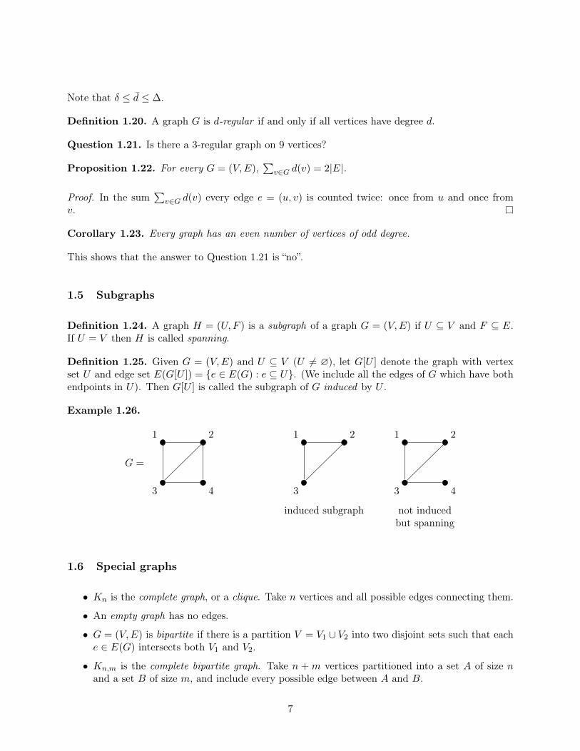
Note that δ ≤ d̄ ≤ ∆.

Definition 1.20. A graph G is d-regular if and only if all vertices have degree d.

Question 1.21. Is there a 3-regular graph on 9 vertices?

Proposition 1.22. For every G = (V,E),∑

v∈G d(v) = 2|E|.

Proof. In the sum∑

v∈G d(v) every edge e = (u, v) is counted twice: once from u and once fromv.

Corollary 1.23. Every graph has an even number of vertices of odd degree.

This shows that the answer to Question 1.21 is “no”.

1.5 Subgraphs

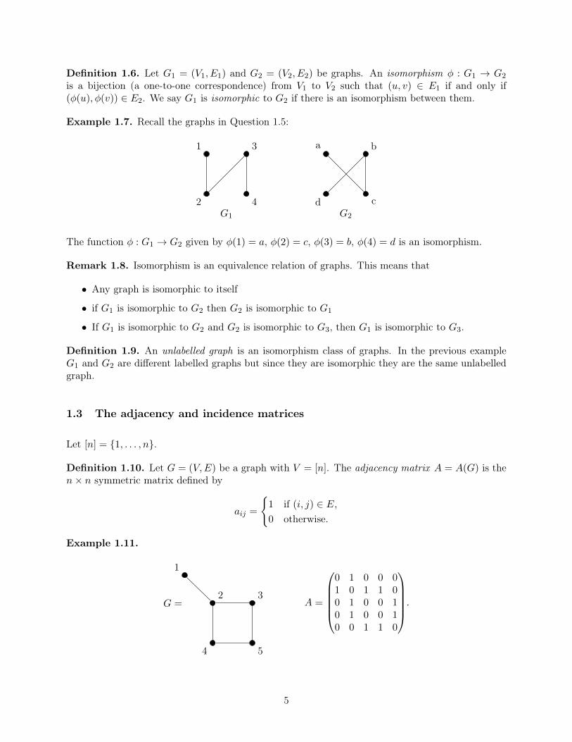
Definition 1.24. A graph H = (U,F ) is a subgraph of a graph G = (V,E) if U ⊆ V and F ⊆ E.If U = V then H is called spanning.

Definition 1.25. Given G = (V,E) and U ⊆ V (U 6= ∅), let G[U ] denote the graph with vertexset U and edge set E(G[U ]) = {e ∈ E(G) : e ⊆ U}. (We include all the edges of G which have bothendpoints in U). Then G[U ] is called the subgraph of G induced by U .

Example 1.26.

3

1

4

2

G =

3

1 2

induced subgraph

3

1

4

2

not inducedbut spanning

1.6 Special graphs

• Kn is the complete graph, or a clique. Take n vertices and all possible edges connecting them.

• An empty graph has no edges.

• G = (V,E) is bipartite if there is a partition V = V1 ∪ V2 into two disjoint sets such that eache ∈ E(G) intersects both V1 and V2.

• Kn,m is the complete bipartite graph. Take n + m vertices partitioned into a set A of size nand a set B of size m, and include every possible edge between A and B.

7

Example 1.27.

K4 = K2,3 =

V1 V2

1.7 Walks, paths and cycles

Definition 1.28. A walk in G is a sequence of vertices v0, v1, v2, . . . , vk, and a sequence of edges(vi, vi+1) ∈ E(G). A walk is a path if all vi are distinct. If for such a path with k ≥ 2, (v0, vk) is alsoan edge in G, then v0, v1, . . . , vk, v0 is a cycle. For multigraphs, we also consider loops and pairs ofmultiple edges to be cycles.

Definition 1.29. The length of a path, cycle or walk is the number of edges in it.

Example 1.30.

v5

v1

v6v2

v3

v4 v5v1v3v4 ≡ path of length 3;

v1v2v3 ≡ cycle of length 3;

v5v1v2v3v1v6 ≡walk of length 5.

Proposition 1.31. Every walk from u to v in G contains a path between u and v.

Proof. By induction on the length ` of the walk u = u0, u1, . . . , v` = v.

If ` = 1 then our walk is also a path. Otherwise, if our walk is not a path there is ui = uj with i < j,then u = u0, . . . , ui, uj+1, . . . , v is also a walk from u to v which is shorter. We can use induction toconclude the proof.

u = u0 u1 ui−1 ui = uj uj+1 v

ui+1uj−1

Proposition 1.32. Every G with minimum degree δ ≥ 2 contains a path of length δ and a cycle oflength at least δ + 1.

8

Proof. Let v1, . . . , vk be a longest path in G. Then all neighbours of vk belong to v1, . . . , vk−1 sok − 1 ≥ δ and k ≥ δ + 1, and our path has at least δ edges. Let i (1 ≤ i ≤ k − 1) be the minimumindex such that (vi, vk) ∈ E(G). Then the neighbours of vk are among vi, . . . , vk−1, so k − i ≥ δ.Then vi, vi+1, . . . , vk is a cycle of length at least δ + 1.

v1 v2 vi vk

Remark 1.33. Note that we have also proved that a graph with minimum degree δ ≥ 2 containscycles of at least δ − 1 different lengths. This fact, and the statement of Proposition 1.32, are bothtight; to see this, consider the complete graph G = Kδ+1.

1.8 Connectivity

Definition 1.34. A graph G is connected if for all pairs u, v ∈ G, there is a path in G from u to v.

Note that it suffices for there to be a walk from u to v, by Proposition 1.31.

Example 1.35.

connected not connected

Definition 1.36. A (connected) component of G is a connected subgraph that is maximal by inclu-sion. We say G is connected if and only if it has one connected component.

Example 1.37.

G =

has 4 connected components.

Proposition 1.38. A graph with n vertices and m edges has at least n−m connected components.

Proof. Start with the empty graph (which has n components), and add edges one-by-one. Note thatadding an edge can decrease the number of components by at most 1.

9

1.9 Graph operations and parameters

Definition 1.39. Given G = (V,E), the complement G of G has the same vertex set V and(u, v) ∈ E

(G)if and only if (u, v) /∈ E(G).

Example 1.40.

3

1

4

2

G =

3

1

4

2

G =

Definition 1.41. A clique in G is a complete subgraph in G. An independent set is an emptyinduced subgraph in G.

Example 1.42.

2

1

4

3

G =

2

1 2

clique in G

1

4

independent setin G

Notation 1.43. Let ω(G) denote the number of vertices in a maximum-size clique in G; let α(G)denote the number of vertices in a maximum-size independent set in G.

Exercise 2. In Example 1.42, ω(G) = 3 and α(G) = 2.

Claim 1.44. A vertex set U ⊆ V (G) is a clique if and only if U ⊆ V(G)is an independent set.

Corollary 1.45. We have ω(G) = α(G)and α(G) = ω

(G).

2 Trees

2.1 Trees

Definition 2.1. A graph having no cycle is acyclic. A forest is an acyclic graph; a tree is a connectedacyclic graph. A leaf (or pendant vertex ) is a vertex of degree 1.

Example 2.2.

10

forest tree

Lemma 2.3. Every finite tree with at least two vertices has at least two leaves. Deleting a leaf froman n-vertex tree produces a tree with n− 1 vertices.

Proof. Every connected graph with at least two vertices has an edge. In an acyclic graph, theendpoints of a maximum path have only one neighbour on the path and therefore have degree 1.Hence the endpoints of a maximum path provide the two desired leaves.

u v

(If v had multiple neighbours on the path we wouldget a cycle).

Suppose v is a leaf of a tree G, and let G′ = G\v. If u,w ∈ V (G′), then no u,w-path P in G canpass through the vertex v of degree 1, so P is also present in G′. Hence G′ is connected. Sincedeleting a vertex cannot create a cycle, G′ is also acyclic. We conclude that G′ is a tree with n− 1vertices.

2.2 Equivalent definitions of trees

Theorem 2.4. For an n-vertex simple graph G (with n ≥ 1), the following are equivalent (andcharacterize the trees with n vertices).

(a) G is connected and has no cycles.

(b) G is connected and has n− 1 edges.

(c) G has n− 1 edges and no cycles.

(d) For every pair u, v ∈ V (G), there is exactly one u, v-path in G.

To prove this theorem we will need a small lemma.

Definition 2.5. An edge of a graph is a cut-edge if its deletion disconnects the graph.

Lemma 2.6. An edge contained in a cycle is not a cut-edge.

Proof. Let (u, v) belong to a cycle.

u u1 u2 uk−1 v

11

Then any path x . . . y in G which uses the edge (u, v) can be extended to a walk in G\(u, v) asfollows:

x u v y

x u u1 uk−1 v y

Proof of Theorem 2.4. We first demonstrate the equivalence of (a), (b), (c) by proving that any twoof {connected, acyclic, n− 1 edges} implies the third.

(a) =⇒ (b), (c): We use induction on n. For n = 1, an acyclic 1-vertex graph has no edge. Forthe induction step, suppose n > 1, and suppose the implication holds for graphs with fewer than nvertices. Given G, Lemma 2.3 provides a leaf v and states that G′ = G\v is acyclic and connected.Applying the induction hypothesis to G′ yields e(G′) = n− 2, and hence e(G) = n− 1.

(b) =⇒ (a), (c): Delete edges from cycles of G one by one until the resulting graph G′ is acyclic.By Lemma 2.6, G is connected. By the paragraph above, G′ has n − 1 edges. Since this equals|E(G)|, no edges were deleted, and G itself is acyclic.

(c) =⇒ (a), (b): Suppose G has k components with orders n1, . . . , nk. Since G has no cycles, eachcomponent satisfies property (a), and by the first paragraph the ith component has ni − 1 edges.Summing this over all components yields e(G) =

∑(ni − 1) = n− k. We are given e(G) = n− 1, so

k = 1, and G is connected.

(a) =⇒ (d): Since G is connected, G has at least one u, v-path for each pair u, v ∈ V (G). SupposeG has distinct u, v-paths P and Q. Let e = (x, y) be an edge in P but not in Q. The concatenationof P with the reverse of Q is a closed walk in which e appears exactly once. Hence, (P ∪Q)\e is anx, y-walk not containing e. By Proposition 1.31, this contains an x, y-path, which completes a cyclewith e and contradicts the hypothesis that G is acyclic. Hence G has exactly one u, v-path.

u v

x y

Q

P

(d) =⇒ (a): If there is a u, v-path for every u, v ∈ V (G), then G is connected. If G has a cycle C,then G has two paths between any pair of vertices on C.

Definition 2.7. Given a connected graph G, a spanning tree T is a subgraph of G which is a treeand contains every vertex of G.

Corollary 2.8.

(a) Every connected graph on n vertices has at least n− 1 edges and contains a spanning tree;

(b) Every edge of a tree is a cut-edge;

(c) Adding an edge to a tree creates exactly one cycle.

12

Proof.

(a) delete edges from cycles of G one by one until the resulting graph G′ is acyclic. By Lemma 2.6,G is connected. The resulting graph is acylic so it is a tree. Therefore G had at least n − 1edges and contained a spanning tree.

(b) note that deleting an edge from a tree T on n vertices leaves n − 2 edges, so the graph isdisconnected by (a).

(c) Let u, v ∈ T . There is a unique path in T between u and v, so adding an edge (u, v) closesthis path to a unique cycle.

u v

2.3 Cayley’s formula

Question 2.9. What is the number of spanning trees in a labelled complete graph on n vertices?

Example 2.10.

1 3

2

n = 3:

1 3

2

1 3

2

n = 4: 4 stars 12 = 4!/2 paths

Theorem 2.11 (Cayley’s Formula). There are nn−2 trees with vertex set [n].

We give two proofs of Cayley’s formula. In our first proof, we establish a bijection between trees on[n] and sequences in [n]n−2.

Definition 2.12 (Prüfer code). Let T be a tree on an ordered set S of n vertices. To compute thePrüfer sequence f(T ), iteratively delete the leaf with the smallest label and append the label of itsneighbour to the sequence. After n − 2 iterations a single edge remains and we have produced asequence f(T ) of length n− 2.

Example 2.13.

2 7 1 4 3

6 8 5

T =

13

We compute the Prüfer code for T as follows:

• 7 (delete 2)

• 4 (delete 3)

• 4 (delete 5)

• 1 (delete 4)

• 7 (delete 6)

• 1 (delete 7)

The edge remaining is (1, 8). We then have f(T ) = (7, 4, 4, 1, 7, 1).

Proposition 2.14. For an ordered n-element set S, the Prüfer code f is a bijection between thetrees with vertex set S and the sequences in Sn−2.

Proof. We need to show every sequence (a1, . . . , an−2) ∈ Sn−2 defines a unique tree T such thatf(T ) = (a1, . . . , an−2). If n = 2, then there is exactly one tree on 2 vertices and the algorithmdefining f always outputs the empty sequence, the only sequence of length zero. So the claim clearlyholds for n = 2.

Now, assume n > 2 and the claim holds for all ordered vertex sets S′ of size less than n. Consider asequence (a1, . . . , an−2) ∈ Sn−2. We need to show that (a1, . . . , an−2) can be uniquely produced bythe algorithm.

Suppose that the algorithm produces f(T ) = (a1, . . . , an−2) for some tree T . Then the vertices{a1, . . . , an−2} are precisely those that are not a leaf in T . Indeed, if a vertex v is a leaf in T thenit can only appear in f(T ) if its neighbour gets deleted during the algorithm. But this would leavev as an isolated vertex, which is impossible. Conversely, if a vertex v is not a leaf then one of itsneighbours must be deleted during the algorithm (it cannot be itself deleted before this happens).When this neighbour of v is deleted, v will be added to the Prüfer code for T , so is in {a1, . . . , an−2}.

This implies that the label of the first leaf removed from T is the minimum element of the setS\{a1, . . . , an−2}. Let v be this element. In other words, in every tree T such that f(T ) =(a1, . . . , an−2) the vertex v is a leaf whose unique neighbour is a1.

By induction, there is a unique tree T ′ with vertex set S\v such that f(T ′) = (a2, . . . , an−2).Adding the vertex v and the edge (a1, v) to T ′ yields the desired unique tree T with f(T ) =(a1, . . . , an−2).

Example 2.15. We use the idea of the above proof to compute the tree with Prüfer code 16631.

2 1

166312 is the smallest leaf

{1, 3, 4, 5, 6, 7} left

14

2 1 6 4


{1, 3, 5, 6, 7} left

2 1 6 4

5


{1, 3, 6, 7} left

2 1 3 6 4

5


{1, 3, 7} left

2 1 3 6 4

5


{1, 7} left

2 1 3 6 4

7 5

Now add an edge betweenthe remaining vertices {1, 7}.

To prove Cayley’s formula, just apply Proposition 2.14 with the vertex set [n] (note that there arenn−2 sequences in [n]n−2).

For our second proof of Cayley’s formula we need the following definition.

Definition 2.16. A directed graph, or digraph for short, is a vertex set and an edge (multi-)set ofordered pairs of vertices. Equivalently, a digraph is a (possibly not-simple) graph where each edgeis assigned a direction. The out-degree (respectively in-degree) of a vertex is the number of edgesincident to that vertex which point away from it (respectively, towards it).

Proof of Cayley’s formula (due to Joyal 1981). We count trees on n vertices which have two distin-guished vertices called the “left end” L and the “right end” R, where L and R can coincide. Let tn

15

be the number of labelled trees on n vertices, and let Tn be the family of labelled trees with twodistinguished vertices L,R. Clearly, |Tn| = tnn

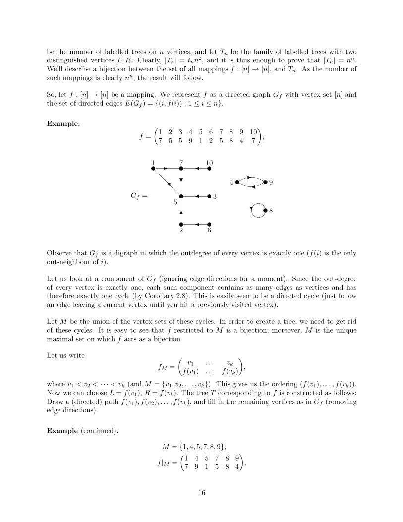
2, and it is thus enough to prove that |Tn| = nn.We’ll describe a bijection between the set of all mappings f : [n] → [n], and Tn. As the number ofsuch mappings is clearly nn, the result will follow.

So, let f : [n] → [n] be a mapping. We represent f as a directed graph Gf with vertex set [n] andthe set of directed edges E(Gf ) = {(i, f(i)) : 1 ≤ i ≤ n}.

Example.

f =

(1 2 3 4 5 6 7 8 9 107 5 5 9 1 2 5 8 4 7

),

1 7 10

53

2 6

4 9

8

Gf =

Observe that Gf is a digraph in which the outdegree of every vertex is exactly one (f(i) is the onlyout-neighbour of i).

Let us look at a component of Gf (ignoring edge directions for a moment). Since the out-degreeof every vertex is exactly one, each such component contains as many edges as vertices and hastherefore exactly one cycle (by Corollary 2.8). This is easily seen to be a directed cycle (just followan edge leaving a current vertex until you hit a previously visited vertex).

Let M be the union of the vertex sets of these cycles. In order to create a tree, we need to get ridof these cycles. It is easy to see that f restricted to M is a bijection; moreover, M is the uniquemaximal set on which f acts as a bijection.

Let us writefM =

(v1 . . . vk

f(v1) . . . f(vk)

),

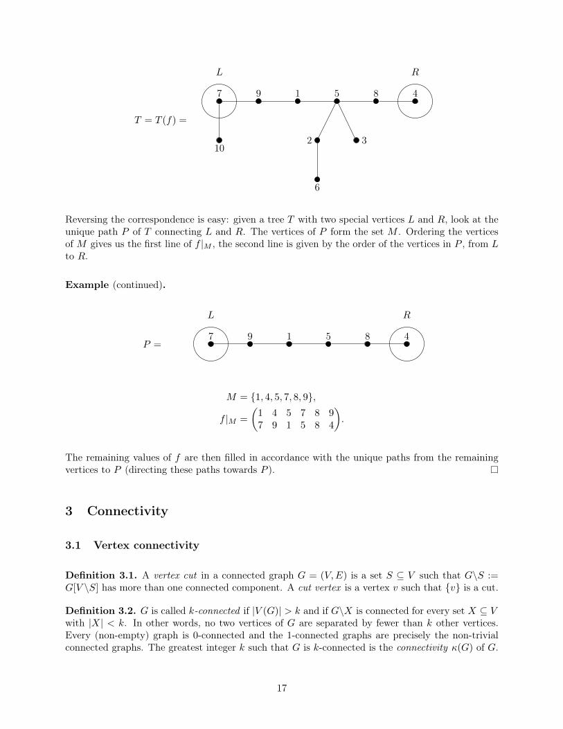
where v1 < v2 < · · · < vk (and M = {v1, v2, . . . , vk}). This gives us the ordering (f(v1), . . . , f(vk)).Now we can choose L = f(v1), R = f(vk). The tree T corresponding to f is constructed as follows:Draw a (directed) path f(v1), f(v2), . . . , f(vk), and fill in the remaining vertices as in Gf (removingedge directions).

Example (continued).

M = {1, 4, 5, 7, 8, 9},

f |M =

(1 4 5 7 8 97 9 1 5 8 4

),

16

7

L

9 1 5 8

R

4

102 3

6

T = T (f) =

Reversing the correspondence is easy: given a tree T with two special vertices L and R, look at theunique path P of T connecting L and R. The vertices of P form the set M . Ordering the verticesof M gives us the first line of f |M , the second line is given by the order of the vertices in P , from Lto R.

Example (continued).

7

L

9 1 5 8

R

4P =

M = {1, 4, 5, 7, 8, 9},

f |M =

(1 4 5 7 8 97 9 1 5 8 4

).

The remaining values of f are then filled in accordance with the unique paths from the remainingvertices to P (directing these paths towards P ).

3 Connectivity

3.1 Vertex connectivity

Definition 3.1. A vertex cut in a connected graph G = (V,E) is a set S ⊆ V such that G\S :=G[V \S] has more than one connected component. A cut vertex is a vertex v such that {v} is a cut.

Definition 3.2. G is called k-connected if |V (G)| > k and if G\X is connected for every set X ⊆ Vwith |X| < k. In other words, no two vertices of G are separated by fewer than k other vertices.Every (non-empty) graph is 0-connected and the 1-connected graphs are precisely the non-trivialconnected graphs. The greatest integer k such that G is k-connected is the connectivity κ(G) of G.

17

• G = Kn: κ(G) = n− 1

• G = Km,n, m ≤ n: κ(G) = m. Indeed, let G have bipartition A ∪ B, with |A| = m and|B| = n. Deleting A disconnects the graph. On the other hand, deleting S ⊂ V with |S| < mleaves both A\S and B\S non-empty and any a ∈ A \S is connected to any b ∈ B \S. HenceG\S is connected.

•v

G = : κ(G) = 1. Deleting v disconnects G, so v is a cut vertex.

Proposition 3.3. For every graph G, κ(G) ≤ δ(G).

Proof. If G is a complete graph then trivially κ(G) = δ(G) = |G| − 1. Otherwise let v ∈ G be avertex of minimum degree d(v) = δ(G). Deleting N(v) disconnects v from the rest of G.

Remark 3.4. High minimum degree does not imply connectivity. Consider two disjoint copies ofKn.

Theorem 3.5 (Mader 1972). Every graph of average degree at least 4k has a k-connected subgraph.

Proof. For k ∈ {0, 1} the assertion is trivial; we consider k ≥ 2 and a graph G = (V,E) with |V | = nand |E| = m. For inductive reasons it will be easier to prove the stronger assertion that G has ak-connected subgraph whenever

(i) n ≥ 2k − 1 and

(ii) m ≥ (2k − 3)(n− k + 1) + 1.

(This assertion is indeed stronger, i.e. (i) and (ii) follow from our assumption of d̄(G) ≥ 4k: (i)holds since n > ∆(G) ≥ 4k, while (ii) follows from m = 1

2 d̄(G)n ≥ 2kn.)

We apply induction on n. If n = 2k − 1, then k = 12(n+ 1), and hence

m ≥ (n− 2)n+ 1

2+ 1 =

1

2n(n− 1)

by (ii). Thus G = Kn ⊇ Kk+1, proving our claim. We therefore assume that n ≥ 2k. If v is a vertexwith d(v) ≤ 2k− 3, we can apply the induction hypothesis to G\v and are done. So we assume thatδ(G) ≥ 2k − 2. If G is itself not k-connected, then there is a separating set X ⊆ V with less thank vertices, such that G\X has two components on the vertex sets V1, V2. Let Gi = G[Vi ∪X], sothat G = G1 ∪G2, and every edge of G is either in G1 or G2 (or both). Each vertex in each Vi hasat least δ(G) ≥ 2k − 2 neighbours in G and thus also in Gi, so |G1|, |G2| ≥ 2k − 1. Note that each|Gi| < n, so by the induction hypothesis, if no Gi has a k-connected subgraph then each

e(Gi) ≤ (2k − 3)(|Gi| − k + 1).

Hence,

m ≤ e(G1) + e(G2)

≤ (2k − 3)(|G1|+ |G2| − 2k + 2)

≤ (2k − 3)(n− k + 1) (since |G1 ∩G2| ≤ k − 1),

contradicting (ii).

18

3.2 Edge connectivity

Definition 3.6. A disconnecting set of edges is a set F ⊆ E(G) such that G \F has more than onecomponent. Given S, T ⊂ V (G), the notation [S, T ] specifies the set of edges having one endpointin S and the other in T . An edge cut is an edge set of the form [S, S], where S is a non-emptyproper subset of V (G). A graph is k-edge-connected if every disconnecting set has at least k edges.The edge-connectivity of G, written κ′(G), is the minimum size of a disconnecting set. One edgedisconnecting G is called a bridge.

Example 3.7.

• G = Kn: κ′(G) = n− 1.

• G = : κ′(G) = 3, whereas κ(G) = 2.

Remark 3.8. An edge cut is a disconnecting set but not the other way around. However, everyminimal disconnecting set is a cut.

Theorem 3.9. κ(G) ≤ κ′(G) ≤ δ(G).

Proof. The edges incident to a vertex v of minimum degree form a disconnecting set; hence κ′(G) ≤δ(G). It remains to show κ(G) ≤ κ′(G). Suppose |G| > 1 and [S, S] is a minimum edge cut, havingsize κ′(G).

If every vertex of S is adjacent to every vertex of S, then κ′(G) = |S||S| = |S|(|G| − |S|). Thisexpression is minimized at |S| = 1. By definition, κ(G) ≤ |G| − 1, so the inequality holds.

Hence we may assume there exists x ∈ S, y ∈ S with x not adjacent to y. Let T be the vertex setconsisting of all neighbours of x in S and all vertices of S\x that have neighbours in S (illustratedbelow). Deleting T destroys all the edges in the cut [S, S] (but does not delete x or y), so T is aseparating set. Now, by the definition of T we can injectively associate at least one edge of

[S, S

]to each vertex in T , so κ(G) ≤ |T | ≤

∣∣[S, S]∣∣ = κ′(G).

x

T

T

T

T

T

y

S S̄

3.3 Blocks

Definition 3.10. A block of a graph G is a maximal connected subgraph of G that has no cut-vertex.If G itself is connected and has no cut-vertex, then G is a block.

19

Example 3.11. If B is a block of G, then B as a graph has no cut-vertex, but B may containvertices that are cut vertices of G. For example, the graph drawn below has five blocks; three copiesof K2, one of K3, and one subgraph that is neither a cycle nor a clique.

Remark 3.12. If a block B has at least three vertices, then B is 2-connected. If an edge is a blockof G then it is a cut-edge of G.

Proposition 3.13. Two blocks in a graph share at most one vertex.

Proof. A single vertex deletion cannot disconnect either block. If blocks B1, B2 share two vertices,then after deleting any single vertex x there remains a path within Bi from every vertex remaining inBi to each vertex of (B1 ∩B2)\x. Hence B1∪B2 is a subgraph with no cut-vertex, which contradictsthe maximality of the original blocks.

Hence the blocks of a graph partition its edge set. When two blocks of G share a vertex, it mustbe a cut-vertex of G. The interaction between blocks and cut-vertices is described by a specialgraph.

Definition 3.14. The block graph of a graph G is a bipartite graph H in which one partite setconsists of the cut-vertices of G, and the other has a vertex bi for each block Bi of G. We include(v, bi) as an edge of H if and only if v ∈ Bi.

Example 3.15.

v1 v2

v3

b1 b3b2

b4

b1

b2

b3

b4

v1

v2

v3

block graph

Proposition 3.16. The block graph of a connected graph is a tree.

Proof. Similar to Proposition 3.13.

20

3.4 2-connected graphs

Definition 3.17. Two paths are internally disjoint if neither contains a non-endpoint vertex of theother. We denote the length of the shortest path from u to v (the distance from u to v) by d(u, v).

Theorem 3.18 (Whitney 1932). A graph G having at least three vertices is 2-connected if and onlyif each pair u, v ∈ V (G) is connected by a pair of internally disjoint u, v-paths in G.

Proof. When G has internally disjoint u, v-paths, deletion of one vertex cannot separate u from v.Since this is given for every u, v, the condition is sufficient. For the converse, suppose that G is2-connected. We prove by induction on d(u, v) that G has two internally disjoint u, v paths. Whend(u, v) = 1, the graph G\(u, v) is connected, since κ′(G) ≥ κ(G) = 2. A u, v-path in G\(u, v) isinternally disjoint in G from the u, v-path consisting of the edge (u, v) itself.

For the induction step, we consider d(u, v) = k > 1 and assume that G has internally disjointx, y-paths whenever 1 ≤ d(x, y) < k. Let w be the vertex before v on a shortest u, v-path. We haved(u,w) = k − 1, and hence by the induction hypothesis G has internally disjoint u,w-paths P andQ. Since G\w is connected, G\w contains a u, v-path R. If this path avoids P or Q, we are finished,but R may share internal vertices with both P and Q. Let x be the last vertex of R belonging toP ∪Q. Without loss of generality, we may assume x ∈ P . We combine the u, x-subpath of P withthe x, v-subpath of R to obtain a u, v-path internally disjoint from Q ∪ {(w, v)}.

u w v

x

Q

PR

Corollary 3.19. G is 2-connected and |G| ≥ 3 if and only if every two vertices in G lie on acommon cycle.

3.5 Menger’s Theorem

Definition 3.20. Let A,B ⊆ V . An A-B path is a path with one endpoint in A, the other endpointin B, and all interior vertices outside of A ∪B. Any vertex in A ∩B is a trivial A-B path.

If X ⊆ V (or X ⊆ E) is such that every A-B path in G contains a vertex (or an edge) from X, wesay that X separates the sets A and B in G. This implies in particular that A ∩B ⊆ X.

Theorem 3.21 (Menger 1927). Let G = (V,E) be a graph and let S, T ⊆ V . Then the maximumnumber of vertex-disjoint S-T paths is equal to the minimum size of an S-T separating vertex set.

21

Proof. Obviously, the maximum number of disjoint paths does not exceed the minimum size of aseparating set, because for any collection of disjoint paths, any separating set must contain a vertexfrom each path. So we just need to prove there is an S-T separating set and a collection of disjointS-T paths with the same size.

We use induction on |E|, the case E = ∅ being trivial. We first consider the case where S and Tare disjoint.

Let k be the minimum size of an S-T separating vertex set. Choose e = (u, v) ∈ E. Let G′ =(V,E \ e). If each S-T separating vertex set in G′ has size at least k, then inductively there exist kvertex-disjoint S-T paths in G′, hence in G.

So we can assume that G′ has an S-T separating vertex set C of size at most k − 1. Then C ∪ {u}and C ∪ {v} are S-T separating vertex sets of G of size k.

Since C is a separating set for G′, no component of G′\C has elements from both S and T . LetVS be the union of components with elements from S, and let VT be the union of components withelements in T . If we were to add the edge (u, v) to G′\C then there would be a path from S to T(because C does not separate S and T in G). So, without loss of generality u ∈ VS and v ∈ VT .

Now, each S-(C ∪{u}) separating vertex set B of G′ has size at least k, as it is S-T separating in G.Indeed, each S-T path P in G intersects C ∪ {u}. Let P ′ be the subpath of P that goes from S tothe first time it touches C ∪ {u}. If P ′ ends with a vertex in C, then u /∈ P so P ′ is an S-(C ∪ {u})path in G′. If P ′ ends in u, then it is disjoint from C and so by the above it contains only verticesin VS . So v /∈ P ′ and again P ′ is an S-(C ∪ {u}) path in G′. In both cases we showed that P ′ is anS-(C ∪ {u}) path in G′ so P intersects B.

So by induction, G′ contains k disjoint S-(C∪{u}) paths. Similarly, G′ contains k disjoint (C∪{v})-T paths. Any path in the first collection intersects any path in the second collection only in C, sinceotherwise G′ contains an S-T path avoiding C.

Hence, as |C| = k − 1, we can pairwise concatenate these paths to obtain k − 1 disjoint S-T paths.We can finally obtain a kth path by inserting the e between the path ending at u and the pathstarting at v.

It remains to consider the general situation where S and T might not be disjoint. Let X = S ∩ Tand apply the theorem with the disjoint sets S′ = S\X and T ′ = T\X, in the graph G′ = G\X. Letk′ be the size of a maximal separating set in G′. We can obtain a (k′ + |X|)-vertex S-T separatingset in G by adding every vertex in X to an S′-T ′ separating set in G′. Similarly we can obtain acollection of k′ + |X| vertex-disjoint S-T paths by adding each vertex in X as a trivial path to acollection of vertex-disjoint S′-T ′ paths in G′.

Corollary 3.22. For S ⊆ V and v ∈ V \ S, the minimum number of vertices distinct from vseparating v from S in G is equal to the maximum number of paths forming an v-S fan in G. (thatis, the maximum number of {v}-S paths which are disjoint except at v).

Proof. Apply Menger’s Theorem with T = N(v). If one of the resulting paths passes through v, itcontains a subpath that is also an S-T path but does not pass through v (note that in such a path, vmust be preceded and succeeded by a vertex of T ). So we have a suitable number of vertex-disjointS-T paths not including v, and we can append v to each path to give a v-S fan.

22

Definition 3.23. The line graph of G, written L(G), is the graph whose vertices are the edges ofG, with (e, f) ∈ E(L(G)) when e = (u, v) and f = (v, w) in G (i.e. when e and f share a vertex).

Example 3.24.

e

f

g

h

G

e

f

g

h

L(G)

Corollary 3.25. Let u and v be two distinct vertices of G.

1. If (u, v) /∈ E, then the minimum number of vertices different from u, v separating u from v inG is equal to the maximum number of internally vertex-disjoint u-v paths in G.

2. The minimum number of edges separating u from v in G is equal to the maximum number ofedge-disjoint u-v paths in G.

Proof. For (i), Apply Menger’s Theorem with S = N(u) and T = N(v).

For (ii), Apply Menger’s Theorem to the line graph of G, with S as the set of edges adjacent to uand T as the set of edges adjacent to v.

Theorem 3.26 (Global Version of Menger’s Theorem).

1. A graph is k-connected if and only if it contains k internally vertex-disjoint paths between anytwo vertices.

2. A graph is k-edge-connected if and only if it contains k edge-disjoint paths between any twovertices.

Proof. First we prove (i). if a graph G contains k internally disjoint paths between any two vertices,then |G| > k and G cannot be separated by fewer than k vertices; thus, G is k-connected.

Conversely, suppose that G is k-connected (and, in particular, has more than k vertices) but containsvertices u, v not linked by k internally disjoint paths. By Corollary 3.25, u and v are adjacent; letG′ = G\(u, v). Then G′ contains at most k − 2 internally disjoint u, v-paths. By Corollary 3.25,we can separate u and v in G′ by a set X of at most k − 2 vertices. As |G| > k, there is at lestone further vertex w /∈ X ∪ {u, v} in G. Now X separates w in G′ from either u or v (say, fromu). But then X ∪ {v} is a set of at most k − 1 vertices separating w from u in G, contradicting thek-connectedness of G.

Then, (ii) follows straight from Corollary 3.25.

23

4 Eulerian and Hamiltonian cycles

4.1 Eulerian trails and tours

Question 4.1. Which of the two pictures below can be drawn in one go without lifting your penfrom the paper?

or

Definition 4.2. A trail is a walk with no repeated edges.

Definition 4.3. An Eulerian trail in a (multi)graph G = (V,E) is a walk in G passing throughevery edge exactly once. If this walk is closed (starts and ends at the same vertex) it is called anEulerian tour.

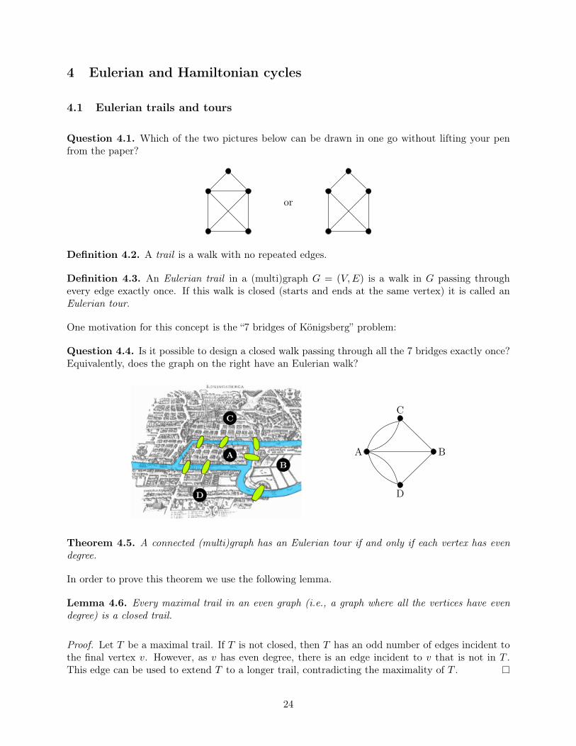
One motivation for this concept is the “7 bridges of Königsberg” problem:

Question 4.4. Is it possible to design a closed walk passing through all the 7 bridges exactly once?Equivalently, does the graph on the right have an Eulerian walk?

AB

C

D

A

C

D

B

Theorem 4.5. A connected (multi)graph has an Eulerian tour if and only if each vertex has evendegree.

In order to prove this theorem we use the following lemma.

Lemma 4.6. Every maximal trail in an even graph (i.e., a graph where all the vertices have evendegree) is a closed trail.

Proof. Let T be a maximal trail. If T is not closed, then T has an odd number of edges incident tothe final vertex v. However, as v has even degree, there is an edge incident to v that is not in T .This edge can be used to extend T to a longer trail, contradicting the maximality of T .

24

Proof of Theorem 4.5. To see that the condition is necessary, suppose G has an Eulerian tour C. Ifa vertex v was visited k times in the tour C, then each visit used 2 edges incident to v (one incomingedge and one outgoing edge). Thus, d(v) = 2k, which is even.

To see that the condition is sufficient, let G be a connected graph with even degrees. Let T =e1e2 . . . e` (where ei = (vi−1, vi)) be a longest trail in G. Then, by Lemma 4.6, T is closed, i.e.,v0 = v`. If T does not include all the edges of G then, since G is connected, there is an edge eoutside of T such that e = (u, vi) for some vertex vi in T . But then T ′ = eei+1 . . . e`e1e2 . . . ei is atrail in G which is longer than T , contradicting the fact that T is a longest trail in G. Thus, weconclude that T includes all the edges of G and so it is an Eulerian tour.

Corollary 4.7. A connected multigraph G has an Eulerian trail if and only if it has either 0 or 2vertices of odd degree.

Proof. Suppose T is an Eulerian trail from vertex u to vertex v. If u = v then T is an Euleriantour and so by Theorem 4.5 it follows that all the vertices in G have even degree. If u 6= v, notethat the multigraph G ∪ {e}, where e = (u, v) is a new edge, has an Eulerian tour, namely T ∪ {e}.By Theorem 4.5 it follows that all the degrees in G ∪ {e} are even. Thus, we conclude that, in theoriginal multigraph G, the vertices u, v are the only ones which have odd degree.

Now we prove the other direction of the corollary. If G has no vertices of odd degree then byTheorem 4.5 it contains an Eulerian tour which is also an Eulerian trail. Suppose now that G has 2vertices u, v of odd degree. Then G ∪ {e}, where e = (u, v) is a new edge, only has vertices of evendegree and so, by Theorem 4.5, it has an Eulerian tour C. Removing the edge e from C gives anEulerian trail of G from u to v.

4.2 Hamilton paths and cycles

Definition 4.8. A Hamilton path/cycle in a graph G is a path/cycle visiting every vertex of Gexactly once. A graph G is called Hamiltonian if it contains a Hamilton cycle.

Hamilton cycles were introduced by Kirkman in 1985, and were named after Sir William Hamilton,who produced a puzzle whose goal was to find a Hamilton cycle in a specific graph.

Example 4.9. Hamilton cycle in the skeleton of the 3-dimensional cube.

We give some necessary conditions for Hamiltonicity.

Proposition 4.10. If G is Hamiltonian then for any set S ⊆ V the graph G\S has at most |S|connected components.

25

Proof. Let C1, . . . , Ck be the components of G\S. Imagine that we are moving along a Hamiltoncycle in some order, vertex-by-vertex (in the picture below, we are moving clockwise, starting fromsome vertex in C1, say). We must visit each component of G\S at least once; when we leave Ci forthe first time, let vi be the subsequent vertex visited (which must be in S). Each vi must be distinctbecause a cycle cannot intersect itself. Hence, S must have at least as many vertices as the numberof connected components of G\S.

S

C3

C2

C4

C1 v1

v3

v4 v2

Corollary 4.11. If a connected bipartite graph G = (V,E) with bipartition V = A∪B is Hamiltonianthen |A| = |B|.

Proof. By deleting the vertices in A from G we get |B| isolated vertices and so G\A has |B| connectedcomponents. Thus, by Proposition 4.10 we conclude that |A| ≥ |B|. By symmetry we can also showthat |B| ≥ |A|. Thus, we conclude that |A| = |B|.

Example 4.12. The condition in Proposition 4.10 is not sufficient to ensure that a graph is Hamil-tonian. The graph G on the right satisfies the condition of Proposition 4.10 but is not Hamiltonian.Indeed, one would need to include all the edges incident to the vertices v1, v2 and v3 in a Hamiltoncycle of G; however, in that case the vertex u would have degree at least 3 in that Hamilton cycle,which is impossible.

v1

v2

v3

u

We also give some sufficient conditions for Hamiltonicity.

Theorem 4.13 (Dirac 1952). If G is a simple graph with n ≥ 3 vertices and if δ(G) ≥ n/2, then Gis Hamiltonian.

Example 4.14. (best-possible minimum degree bound):

26

• The graph consisting of two cliques of orders b(n+ 1)/2c and d(n+ 1)/2e sharing a vertex hasminimum degree b(n− 1)/2c but is not Hamiltonian (it is not even 2-connected).

Kb(n+1)/2c Kd(n+1)/2e

• If n is odd, then the complete bipartite graph K(n−1)/2,(n+1)/2 has minimum degree n−12 but

is not Hamiltonian.

Proof of Theorem 4.13. The condition that n ≥ 3 must be included since K2 is not Hamiltonian butsatisfies δ(K2) = |K2|/2.

If there is a non-Hamiltonian graph satisfying the hypotheses, then adding edges cannot reducethe minimum degree, so we may restrict our attention to maximal non-Hamiltonian graphs G withminimum degree at least n/2. By “maximal" we mean that for every pair (u, v) of non-adjacentvertices of G, the graph obtained from G by adding the edge e = (u, v) is Hamiltonian.

The maximality of G implies that G has a Hamilton path, say from u = v1 to v = vn, becauseevery Hamilton cycle in G ∪ {e} must contain the new edge e. We use most of this path v1, . . . , vn,with a small switch, to obtain a Hamilton cycle in G. If some neighbour of u immediately follows aneighbour of v on the path, say (u, vi+1) ∈ E(G) and (v, vi) ∈ E(G), then G has the Hamilton cycle(u, vi+1, vi+2, . . . , vn−1, v, vi, vi−1, . . . , v2) shown below.

u vi vi+1 v

To prove that such a cycle exists, we show that there is a common index in the sets S and T definedby S = {i : (u, vi+1) ∈ E(G)} and T = {i : (v, vi) ∈ E(G)}. Summing the sizes of these sets yields

|S ∪ T |+ |S ∩ T | = |S|+ |T | = d(u) + d(v) ≥ n.

Neither S nor T contains the index n. This implies that |S ∪ T | < n, and hence |S ∩ T | ≥ 1, asrequired. This is a contradiction.

Ore observed that this argument uses only that d(u) + d(v) ≥ n. Therefore, we can weaken therequirement of minimum degree n/2 to require only that d(u)+d(v) ≥ n whenever u is not adjacentto v.

Theorem 4.15 (Ore 1960). If G is a simple graph with n ≥ 3 vertices such that for every pair ofnon-adjacent vertices u, v of G we have d(u) + d(v) ≥ |G|, then G is Hamiltonian.

27

5 Matchings

Definition 5.1. A set of edges M ⊆ E(G) in a graph G is called a matching if e ∩ e′ = ∅ for anypair of edges e, e′ ∈M .

A matching is perfect if |M | = |V (G)|2 , i.e. it covers all vertices of G. We denote the size of the

maximum matching in G, by ν(G).

Example 5.2.

• G = Kn: ν(G) =⌊n2

⌋• G = Ks,t, s ≤ t: ν(G) = s

• G = : ν(G) = 5

Remark 5.3. A matching in a graph G corresponds to an independent set in the line graph L(G)

Definition 5.4. A set of vertices T ⊆ V (G) of a graph G is called a cover of G if every edgee ∈ E(G) intersects T (e ∩ T 6= ∅), i.e., G \ T is an empty graph. Then, τ(G) denotes the size ofthe minimum cover.

Example 5.5.

• G = Kn: τ(G) = n− 1

• G = Ks,t, s ≤ t: ν(G) = s

•⊗

⊗⊗⊗ ⊗

⊗

G = : τ(G) = 6.

To see this, note that the graphs induced by the outer 5 vertices and inner 5 vertices are both5-cycles C5. Since τ(C5) = 3, at least 3 of the outer vertices and 3 of the inner vertices mustbe included in a vertex cover.

Proposition 5.6. ν(G) ≤ τ(G) ≤ 2ν(G).

Proof. Let M be a maximum matching in G. Since every cover has at least one vertex on each edgeof M and edges are disjoint, we have ν(G) ≤ τ(G). Note also that since M is maximum, every edgee ∈ E(G) intersects some edge e′ ∈M , otherwise we get a larger matching. So the vertices coveredby M form a cover for G, hence τ(G) ≤ 2|M | = 2ν(G).

28

5.1 Real-world applications of matchings

Here is just a short list of situations where it is useful to think about and look for matchings.

• Suppose certain workers can operate certain machines, but only one at a time; this gives abipartite graph between workers and machines. If we want to have many machines operatingat the same time, we need a large matching in our bipartite graph.

• Suppose we have a number of hour-long jobs to perform on two computers. Certain jobs canonly be started once other jobs are finished. We can define a graph by putting an edge betweenevery pair of jobs that can be performed simultaneously; to finish all the jobs as quickly aspossible we would like to find a large matching in our graph.

• The molecular structure of a compound can be described by a graph. For certain kinds ofhydrocarbon molecules (benzenoids), a perfect matching of this graph gives information aboutthe location of its “double bonds”.

• When students apply to universities, each student has a list of university preferences, andeach university also has a list of preferences for students. In order to decide which studentsshould go to which university, we need to find a bipartite matching that is somehow compatiblewith these preferences. This kind of situation is called the stable matching problem, and isextremely important in economics and operations research. The Gale-Shapley algorithm forefficiently computing a stable matching was worth the Nobel prize in economics in 2012.

• Algorithms to find large matchings are essential subroutines for solving optimization problems.The Chinese postman problem involves visiting several designated points while travelling asshort a total distance as possible. This problem can be efficiently solved by first solving a setof shortest path problems, then solving a certain matching problem.

5.2 Hall’s Theorem

Theorem 5.7 (Hall 1935). A bipartite graph G = (V,E) with bipartition V = A∪B has a matchingcovering A if and only if

|N(S)| ≥ |S| ∀S ⊆ A. (1)

Proof. It is easy to see that if G has such a matching then (1) holds.

To show the other direction, we apply induction on |A|. For |A| = 1 the assertion is true. Now let|A| ≥ 2, and assume that (1) is sufficient for the existence of a matching covering A when |A| issmaller.

If |N(S)| ≥ |S| + 1 for every non-empty set S $ A, then we pick an edge (a, b) ∈ G and considerthe graph G′ = G\{a, b} obtained by deleting the vertices a and b. Then every non-empty setS ⊆ A \ {a} satisfies

|NG′(S)| ≥ |NG(S)| − 1 ≥ |S|,

so by the induction hypothesis G′ contains a matching covering A \ {a}. Together with the edge ab,this yields a matching covering A in G.

Suppose now that A has a non-empty proper subset A′ with neighbourhood B′ = N(A′) suchthat |A′| = |B′|. By the induction hypothesis, G′ = G[A′ ∪ B′] contains a matching covering

29

A′. But G\G′ satisfies (1) as well: for any set S ⊆ A \ A′ with |NG\G′(S)| < |S| we would have|NG(S ∪ A′)| = |NG\G′(S)| + |B′| < |S ∪ A′|, contrary to our assumption. Again, by induction,G\G′ contains a matching of A \ A′. Putting the two matchings together, we obtain a matching inG covering A.

The next corollary gives a so-called defect version of Hall’s theorem.

Corollary 5.8. If in a bipartite graph G = (A∪B,E) we have |N(S)| ≥ |S|−d for every set S ⊆ Aand some fixed d ∈ N, then G contains a matching of cardinality |A| − d.

Proof. We add d new vertices to B, joining each of them to all the vertices in A. Call the resultinggraph G′. Note that the new graph has

NG′(S) ≥ |NG(S)|+ d ≥ |S| − d+ d = |S|

for any S ⊆ A, so by Hall’s theorem, G′ contains a matching of A. At least |A| − d edges in thismatching must be edges of G.

Corollary 5.9. If a bipartite graph G = (A ∪ B,E) is k-regular with k ≥ 1, then G has a perfectmatching.

Proof. IfG is k-regular, then clearly |A| = |B|, since the total number of edges is k|A| =∑

x∈A d(x) =∑y∈B d(y) = k|B|. It thus suffices to show by Theorem 5.7 that G contains a matching covering A.

Now every set S ⊆ A is joined to N(S) by a total of k|S| edges, and these are among the k|N(S)|edges of G incident with N(S). Therefore k|S| ≤ k|N(S)|, so G does indeed satisfy (1).

Corollary 5.10. Every regular graph of positive even degree has a 2-factor (a spanning 2-regularsubgraph).

Proof. let G be any connected 2k-regular graph. By Theorem 4.5 G contains an Euler tour. Definea new graph G′ by splitting every vertex v into two vertices v− and v+. If an edge of the Eulertour goes from v to w, put an edge in G′ from v+ to w−. So, the edges in G and in G′ naturallycorrespond to each other. It is easy to see that G′ is bipartite and k-regular so contains a perfectmatching. Collapsing each pair of vertices v−,v+ back into a single vertex v, a perfect matching ofG′ corresponds to a 2-factor of G. (Each vertex v is incident to one edge which was incident to v+

in G′, and one edge incident to v− in G′).

Remark 5.11. A 2-factor is a disjoint union of cycles covering all the vertices of a graph

Definition 5.12. Let A1, . . . , An be a collection of sets. A family {a1, . . . , an} is called a system ofdistinct representatives (SDR) if all the ai are distinct, and ai ∈ Ai for all i.

Corollary 5.13. A collection A1, . . . , An has an SDR if and only if for all I ⊆ [n] we have|⋃i∈I Ai| ≥ |I|.

Proof. Define a bipartite graph with parts A = [n] and X =⋃iAi such that (i, a) is an edge if and

only if a ∈ Ai. A matching of [n] in this graph corresponds exactly to an SDR, where an edge (i, a)in the matching means that ai = a. But the condition |

⋃i∈I Ai| ≥ |I| for all I ⊆ [n] is precisely

Hall’s condition for the existence of a matching covering A, so Hall’s theorem provides the desiredequivalence.

30

Example 5.14. A1 = {1, 2}, A2 = {1, 2, 3}, A3 = {4}, A4 = {1, 3, 4}.

A1 A2 A3 A4

1 2 3 4

Theorem 5.15 (Kőnig 1931). If G = (A ∪ B,E) is a bipartite graph, then the maximum size of amatching in G equals the minimum size of a vertex cover of G.

Proof. We have already seen that a minimum cover has at least the size of a maximum matching.Now take a minimum vertex cover U of G. We construct a matching of size |U | to prove that equalitycan always be achieved.

Let R = U ∩ A and T = U ∩ B. Let H,H ′ be the subgraphs of G induced by R ∪ (B\T ) andT ∪ (A\R). We use Hall’s theorem to show that H has a complete matching of R into B\T andH ′ has a complete matching of T into A\R. Since these subgraphs are disjoint, the two matchingstogether form a matching of size |U | in G.

Since R ∪ T is a vertex cover, G has no edge from B\T to A\R. Suppose S ⊆ R, and considerNH(S) ⊆ B\T . If |NH(S)| < |S|, then we can substitute NH(S) for S in U and obtain a smallervertex cover, since NH(S) covers all edges incident to S that are not covered by T . The minimalityof U thus implies that Hall’s condition holds in H, and hence H has a complete matching of R intoB\T . Applying the same argument to H ′ yields the rest of the matching.

A R

B T

H ′ H

5.3 Matchings in general graphs: Tutte’s Theorem

Given a graph G, let q(G) denote the number of its odd components, i.e. the ones of odd order. IfG has a perfect matching then clearly

q(G\S) ≤ |S| for all S ⊆ V (G), (2)

since every odd component of G\S will send an edge of the matching to S, and each such edge coversa different vertex in S.

31

S

G\S

Theorem 5.16 (Tutte, 1947). A graph G has a perfect matching if and only if q(G\S) ≤ |S| forall S ⊆ V (G).

Proof. As noted above, Tutte’s condition is necessary; we prove sufficiency. Tutte’s condition ispreserved by addition of edges: if G′ = G ∪ {e} and S ⊆ V (G), then q(G′\S) ≤ q(G\S), becausewhen the addition of e combines two components of G\S into one, the number of components thathave odd order does not increase. Therefore, it suffices to consider a simple graph G such that Gsatisfies (2), has no perfect matching, but adding any edge to G creates a perfect matching. We willobtain a contradiction in every case by constructing a perfect matching in G.

By considering S = ∅, we know that G has an even number of vertices, since a graph of odd ordermust have a component of odd order. Let U be the set of vertices in G that are connected to allother vertices. Suppose G\U consists of disjoint complete graphs; we build a perfect matching forsuch a G. The vertices in each component of G\U can be paired up arbitrarily, with one left overin the odd components. Since q(G\U) ≤ |U | and each vertex of U is adjacent to all of G\U , we canmatch these leftover vertices arbitrarily to vertices in U to complete a matching.

This leaves the case where G\U is not a disjoint union of cliques. We can therefore find two verticesin the same component which are not adjacent, and on a shortest path between them there are twononadjacent vertices x, z at distance 2 (which have a common neighbour y). Furthermore, G\U hasanother vertex w not adjacent to y, since y 6∈ U . By the maximality of G, adding any edge to Gproduces a perfect matching. Let M1 and M2 be perfect matchings in G ∪ (x, z) and G ∪ (y, w),respectively. It suffices to show that in M1 ∪M2 we can find a perfect matching avoiding (x, z) and(y, w), because that would be contained in G.

Let F be the graph on V (G) with the edges that belong to exactly one of M1 and M2. Note that Fcontains (x, z) and (y, w). Since every vertex of G has degree 1 in each of M1 and M2, every vertexof G has degree 0 or 2 in F . Hence F is a collection of disjoint even cycles (alternating betweenedges of M1 and M2) and isolated vertices. Let C be the cycle of F containing (x, z). If C does notalso contain (y, w), then the desired matching consists of the edges of M2 from C and all of M1 notin C. If C contains both (y, w) and (x, z), as illustrated below, then we use the edge (y, x) or theedge (y, z) to obtain a matching of V (C) using only edges of G (avoiding both (x, z) and (y, w)).Specifically, we use (y, x) if the distance between y and x in C is odd, and we use (y, z) otherwise(then the distance between y and z in C is odd). In the illustration below, this second case applies.The remaining vertices of C form two paths of even order. We use the edges of M1 in one of thesepaths and the edges ofM2 in the other to produce a matching in C that does not use (x, z) or (y, w).(In the illustration below, we use the edges of M1 on the right side of (y, z) and the edges of M2 onthe left). Combined with M1 or M2 outside C, we have a perfect matching of G.

32

M2 M1 M2

M2 M1 M2

M1 M1

x z

y w

Corollary 5.17 (Petersen, 1891). Every 3-regular graph with no cut-edge has a perfect matching.

Proof. Let S ⊆ V (G). Let H be a component of G\S, with |H| odd. The number of edges betweenS and H cannot be 1, since G has no cut-edge. It also cannot be even, because then the sum of thevertex degrees in H would be odd. Hence there are at least three edges from H to S.

Since G is 3-regular, each vertex of S is incident to at most three edges between S and G\S.Combining this fact with the previous paragraph, we have 3q(G\S) ≤ 3|S| and hence q(G\S) ≤ |S|,which proves the corollary.

Example 5.18. The condition that the graph has no cut-edge is necessary. The graph below is3-regular but has no perfect matching. Deleting the central vertex leaves 3 odd components.

Finally, we give a defect version of Tutte’s theorem.

Corollary 5.19 (Berge 1958). The largest matching in an n-vertex graph G covers n+minS⊆V (G)(|S| − q(G\S))vertices.

Proof. Let d(S) = q(G\S)− |S| and let d = maxS⊆V d(S). Given S ⊆ V (G), at most |S| edges canmatch vertices of S to vertices in odd components of G\S, so every matching has at least q(G\S)−|S|unmatched vertices. We have shown that no matching can have more than n− d vertices; we wantto achieve this bound. Considering the case S = ∅ shows d ≥ 0. Let G′ be obtained by addinga set D of d vertices to G, each of which are adjacent to every other vertex. Since d(S) has thesame parity as |G| for each S, we know that |G′| is even. If G′ satisfies Tutte’s condition, then wecan obtain a matching of the desired size in G from a perfect matching in G′, because deleting Deliminates edges that match at most d vertices of G.

The condition q(G′\S′) ≤ |S′| holds for S′ = ∅ because |G′| is even. If S′ is nonempty but doesnot contain all of D, then G′\S′ has only one component, and 1 ≤ |S′|. Finally, if D ⊆ S′, letS = S′\D. We have G′\S′ = G\S, so q(G′\S′) = q(G\S) ≤ |S| + d = |S′|, and G′ indeed satisfiesTutte’s condition.

33

6 Planar Graphs

Definition 6.1. A polygonal path or polygonal curve in the plane is the union of many line segmentssuch that each segment starts at the end of the previous one and no point appears in more thanone segment except for common endpoints of consecutive segments. In a polygonal u, v-path, thebeginning of the first segment is u and the end of the last segment is v.

A drawing of a graph G is a function that maps each vertex v ∈ V (G) to a point f(v) in the planeand each edge uv to a polygonal f(u), f(v)-path in the plane. The images of vertices are distinct.A point in f(e)∩ f(e′) other than a common end is a crossing. A graph is planar if it has a drawingwithout crossings. Such a drawing is a planar embedding of G. A plane graph is a particular drawingof a planar graph in the plane with no crossings.

Example 6.2.

K4 planar drawing

Remark 6.3. We get the same class of graphs if we only require images of edges to be continuouscurves. This is because any continuous line can be arbitrarily accurately approximated by a polygonalcurve.

Definition 6.4. An open set in the plane is a set U ⊂ R2 such that for every p ∈ U , all pointswithin some small distance from p belong to U . A region is an open set U that contains a polygonalu, v-path for every pair u, v ∈ U (that is, it is “path-connected”). The faces of a plane graph are themaximal regions of the plane that are disjoint from the drawing.

Theorem 6.5 (Jordan curve theorem). A simple closed polygonal curve C consisting of finitelymany segments partitions the plane into exactly two faces, each having C as boundary.

Remark 6.6. This is not true in three dimensions. In R3 there is a surface called the Möbius bandwhich has only one side.

Remark 6.7. The faces of G are pairwise disjoint (they are separated by the edges of G). Twopoints are in the same face if and only if there is a polygonal path between them which does notcross an edge of G. Also, note that a finite graph has a single unbounded face (the area “outside” ofthe graph).

Proposition 6.8. A plane forest has exactly one face.

Definition 6.9. The length of the face f in a planar embedding of G is the length of the walk in Gthat bounds it.

Example 6.10. The following graph has 3 faces of lengths 6,3 and 7.

34

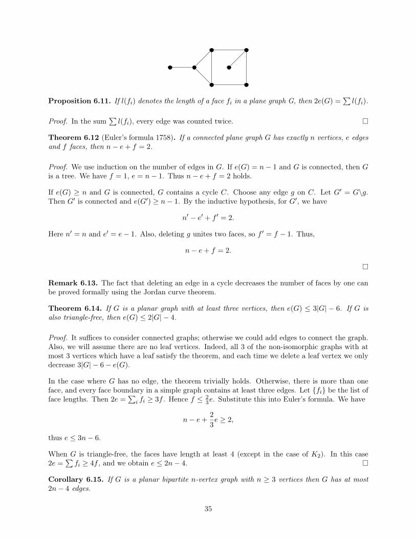
Proposition 6.11. If l(fi) denotes the length of a face fi in a plane graph G, then 2e(G) =∑l(fi).

Proof. In the sum∑l(fi), every edge was counted twice.

Theorem 6.12 (Euler’s formula 1758). If a connected plane graph G has exactly n vertices, e edgesand f faces, then n− e+ f = 2.

Proof. We use induction on the number of edges in G. If e(G) = n− 1 and G is connected, then Gis a tree. We have f = 1, e = n− 1. Thus n− e+ f = 2 holds.

If e(G) ≥ n and G is connected, G contains a cycle C. Choose any edge g on C. Let G′ = G\g.Then G′ is connected and e(G′) ≥ n− 1. By the inductive hypothesis, for G′, we have

n′ − e′ + f ′ = 2.

Here n′ = n and e′ = e− 1. Also, deleting g unites two faces, so f ′ = f − 1. Thus,

n− e+ f = 2.

Remark 6.13. The fact that deleting an edge in a cycle decreases the number of faces by one canbe proved formally using the Jordan curve theorem.

Theorem 6.14. If G is a planar graph with at least three vertices, then e(G) ≤ 3|G| − 6. If G isalso triangle-free, then e(G) ≤ 2|G| − 4.

Proof. It suffices to consider connected graphs; otherwise we could add edges to connect the graph.Also, we will assume there are no leaf vertices. Indeed, all 3 of the non-isomorphic graphs with atmost 3 vertices which have a leaf satisfy the theorem, and each time we delete a leaf vertex we onlydecrease 3|G| − 6− e(G).

In the case where G has no edge, the theorem trivially holds. Otherwise, there is more than oneface, and every face boundary in a simple graph contains at least three edges. Let {fi} be the list offace lengths. Then 2e =

∑i fi ≥ 3f . Hence f ≤ 2

3e. Substitute this into Euler’s formula. We have

n− e+2

3e ≥ 2,

thus e ≤ 3n− 6.

When G is triangle-free, the faces have length at least 4 (except in the case of K2). In this case2e =

∑fi ≥ 4f , and we obtain e ≤ 2n− 4.

Corollary 6.15. If G is a planar bipartite n-vertex graph with n ≥ 3 vertices then G has at most2n− 4 edges.

35

Corollary 6.16. K5 and K3,3 are not planar.

K3,3 K5

Proof. K5 is a non-planar graph since e = 10 > 9 = 3n − 6. K3,3 is a non-planar graph sincee = 9 > 8 = 2n− 4.

Remark 6.17 (Maximal planar graphs / triangulations). The proof of Theorem 6.14 shows thathaving 3n− 6 edges in a simple n-vertex planar graph requires 2e = 3f , meaning that every face isa triangle. If G has some face that is not a triangle, then we can add an edge between non-adjacentvertices on the boundary of this face to obtain a larger plane graph. Hence the simple plane graphswith 3n− 6 edges, the triangulations, and the maximal plane graphs are all the same family.

6.1 Platonic Solids

Definition 6.18. A polytope is a solid in 3 dimensions with flat faces, straight edges and sharpcorners. Faces of a polytope are joined at the edges. A polytope is convex if the line connecting anytwo points of the polytope lies inside the polytope.

Example 6.19. The tetrahedron:

Definition 6.20. A regular or Platonic solid is a convex polytope which satisfies the following:

1. all of its faces are congruent regular polygons,

2. all vertices have the same number of faces adjacent to them.

We will now characterise all Platonic solids. The first step is to convert a convex polytope into aplanar graph. To do this, we place the considered polytope inside a sphere. Then we project thepolytope onto the sphere (imagine that the edges of the polytope are made from wire and we placea tiny lamp in the center). This yields a graph drawn on the sphere without edge crossings.

Now let us show that planar graphs are exactly graphs that can be drawn on the sphere. This becomesquite obvious if we use the stereographic projection. We place the sphere in the 3-dimensional spacein such a way that it touches the considered plane ρ. Let o denote the point of the sphere lyingfarthest from ρ, the ’north pole’.

36

o

x

x′

ρ

Then the stereographic projection maps each point x 6= o of the sphere to a point x′, where x′ isthe intersection of the line ox with the plane ρ. (For the point o, the projection is undefined.) Thisdefines a bijection between the plane and the sphere without the point o. Given a drawing of a graphG on the sphere without edge crossings, where the point o lies on no arc of the drawing (which wemay assume by a suitable choice of o), the stereographic projection yields a planar drawing of G.Conversely, from a planar drawing we get a drawing on the sphere by the inverse projection.

Corollary 6.21. If K is a convex polytope with v vertices, e edges and f faces then v − e+ f = 2.

Suppose K is a Platonic solid. All its faces are congruent; assume that they have n vertices (and,thus, n edges). Let us assume moreover that each vertex is adjacent to m faces (and, thus, it has medges adjacent to it). Since each edge is adjacent to exactly two faces,

2e = nf. (3)

Moreover, each edge is adjacent to two vertices, and one vertex belongs to m edges, thus

mv = 2e. (4)

Expressing v and f in terms of e, and substituting to Euler’s formula, we obtain that2e

m−e+

2e

n= 2.

Rearranging, we arrive at1

m+

1

n=

1

2+

1

e.

Note that since K is a 3-dimensional polytope, each of its faces is a polygon and thus has at least 3vertices, that is n ≥ 3. Moreover, at each vertex, there are at least three faces meeting; m ≥ 3. Onthe other hand, since e ≥ 1, we must have

1

m+

1

n>

1

2. (5)

These conditions do not leave too much leeway; there are only five possible (n,m) pairs for whichthe above inequality holds. These are (3, 3), (3, 4), (3, 5), (4, 3), (5, 3).

A Platonic solid corresponds to each of these pairs. We list them below.

37

• Tetrahedron. Here n = 3 and m = 3. Thus, (5) yields that e = 6. By (4), v = 4, and by (3),f = 4. There are 4 vertices and 4 faces of the tetrahedron; the faces are regular triangles, andthe vertices are adjacent to 3 edges.

• Octahedron. Here n = 3 and m = 4. Thus, (5) yields that e = 12. By (4), v = 6, and by(3), f = 8. There are 8 vertices and 8 faces of the octahedron; the faces are regular triangles,and the vertices are adjacent to 4 edges.

• Icosahedron. Here n = 3 and m = 5. Thus, (5) yields that e = 30. By (4), v = 12, andby (3), f = 20. There are 12 vertices and 20 faces of the icosahedron; the faces are regulartriangles, and the vertices are adjacent to 5 edges.

• Cube. Here n = 4 and m = 3. Thus, (5) yields that e = 12. By (4), v = 8, and by (3), f = 6.There are 8 vertices and 6 faces of the tetrahedron; the faces are squares, and the vertices areadjacent to 3 edges.

• Dodecahedron. Here n = 5 and m = 3. Thus, (5) yields that e = 30. By (4), v = 20, andby (3), f = 12. There are 20 vertices and 12 faces of the tetrahedron; the faces are regularpentagons, and the vertices are adjacent to 3 edges.

7 Graph colouring

7.1 Vertex colouring

Definition 7.1. A k-colouring of G is a labeling f : V (G)→ {1, . . . , k}. It is a proper k-colouringif (x, y) ∈ E(G) implies f(x) 6= f(y). A graph G is k-colourable if it has a proper k-colouring. Thechromatic number χ(G) is the minimum k such that G is k-colourable. If χ(G) = k, then G isk-chromatic. If χ(G) = k, but χ(H) < k for every proper subgraph H of G, then G is colour-criticalor k-critical.

Example 7.2.

• χ(Kn) = n

• G = : χ(G) = 4

• The chromatic number of an odd cycle is 3

38

Remark 7.3. The vertices having a given colour in a proper colouring must form an independent set,so χ(G) is the minimum number of independent sets needed to cover V (G). Hence G is k-colourableif and only if G is k-partite. Multiple edges do not affect chromatic number. Although we definek-colouring using numbers from {1, . . . , k} as labels, the numerical values are usually unimportant,and we may use any set of size k as labels.

7.2 Some motivation

Example 7.4 (examination scheduling). The students at a certain university have annual exam-inations in all the courses they take. Naturally, examinations in different courses cannot be heldconcurrently if the courses have students in common. How can all the examinations be organizedin as few parallel sessions as possible? To find a schedule, consider the graph G whose vertex setis the set of all courses, two courses being joined by an edge if they give rise to a conflict. Clearly,independent sets of G correspond to conflict-free groups of courses. Thus, the required minimumnumber of parallel sessions is the chromatic number of G.

Example 7.5 (chemical storage). A company manufactures n chemicals C1, C2, . . . , Cn. Certainpairs of these chemicals are incompatible and would cause explosions if brought into contact witheach other. As a precautionary measure, the company wishes to divide its warehouse into com-partments, and store incompatible chemicals in different compartments. What is the least numberof compartments into which the warehouse should be partitioned? We obtain a graph G on thevertex set {v1, v2, . . . , vn} by joining two vertices vi and vj if and only if the chemicals Ci and Cjare incompatible. It is easy to see that the least number of compartments into which the warehouseshould be partitioned is equal to the chromatic number of G.

7.3 Simple bounds on the chromatic number

Claim 7.6. If H is a subgraph of G then χ(H) ≤ χ(G).

Proof. Note that a proper colouring of G is also a proper colouring of H.

Corollary 7.7. χ(G) ≥ ω(G)

Proof. Let ω(G) = t. Then G contains a subgraph H which is isomorphic to Kt. Thus, by the claimabove it follows that χ(G) ≥ χ(H) = t.

Example 7.8. Consider the following graph.

G =

In this case we have χ(G) = 4 and ω(G) = 3. Thus, the chromatic number can be bigger than theclique number.

39

Proposition 7.9. χ(G) ≥ |V (G)|α(G)

Proof. Let χ(G) = k. A k-colouring of V (G) gives a partition V (G) = V1 ∪ . . . ∪ Vk such thatevery Vi is an independent set. Hence, |Vi| ≤ α(G). Therefore, |V (G)| =

∑ki=1 |Vi| ≤ kα(G). Thus,

k = χ(G) ≥ |V (G)|α(G) as claimed.

Claim 7.10. For any graph G = (V,E) and any U ⊆ V we have χ(G) ≤ χ(G[U ]) + χ(G[V \ U ]).

Proof. Properly colour U using χ(G[U ]) colours and properly colour V \U using χ(G[V \U ]) othercolours. This gives a proper colouring of G in χ(G[U ]) + χ(G[V \ U ]) colours.

Claim 7.11. For any graphs G1 and G2 on the same vertex set, χ(G1 ∪G2) ≤ χ(G1)χ(G2).

Proof. Let c1 and c2 be colourings of G1 and G2 with the integers in [χ(G1)] and [χ(G2)] respectively.We colour the vertices of G1 ∪ G2 with elements of the set [χ(G1)] × [χ(G2)], with the colouring cdefined by c(v) = (c1(v), c2(v)). If v is adjacent to w in G1 ∪G2 then (v, w) is an edge in one of G1

or G2, so c1(v) 6= c1(w) or c2(v) 6= c2(w). This proves that c(v) 6= c(w), so c is proper.

Proposition 7.12.

(i) χ(G)χ(G)≥ |G|

(ii) χ(G) + χ(G)≤ |G|+ 1

Proof. (i) follows from Claim 7.11: we have χ(G)χ(G)≥ χ

(G ∪G

)= χ

(K|G|

)= |G|.

(ii) can be proved by induction on |G| (the case |G| = 1 is obvious). So, let |G| = n + 1. LetG0 = G\v for some vertex v. By induction we have χ(G0) + χ

(G0

)≤ n + 1. Let c : V → [k] be a

colouring of G0 and f : V → [`] be a colouring of G0, with k + ` = n+ 1 (we might be using morecolours than are necessary). If dG(v) < k then there is a colour cv such that v has no neighbourscoloured cv. We can then colour v with cv to extend c to a colouring of G with k colours. This wouldprove χ(G) ≤ k, and since χ

(G)

= χ(G0 ∪ {v}

)≤ `+ 1 we have χ(G) + χ

(G)≤ k + `+ 1 ≤ n+ 2.

Otherwise dG(v) ≥ k so dG(v) ≤ n − k = ` − 1. We can then use exactly the same reasoning asbefore to extend f to a colouring of G with ` colours, and since χ(G) ≤ k+ 1 we are done again.

7.4 Greedy colouring

Definition 7.13. The greedy colouring with respect to a vertex ordering v1, . . . , vn of V (G) isobtained by colouring vertices in the order v1, . . . , vn, assigning to vi the smallest-indexed colour notalready used on its lower-indexed neighbours.

Example 7.14.

40

v1 v3 v5

v2 v4

This graph has chromatic number 2 but the greedy colouring needs 3 colours.

Definition 7.15. Let G = (V,E) be a graph. We say that G is k-degenerate if every subgraph ofG has a vertex of degree less than or equal to k.

Proposition 7.16. G is k-degenerate if and only if there is an ordering v1, . . . , vn of the vertices ofG such that each vi has at most k neighbours among the vertices v1, . . . , vi−1.

Proof. If there is such an ordering, then for any subgraph H, consider the maximum vertex of Hwith respect to the ordering. This vertex has at most k neighbours in H, thus proving that G isk-degenerate.

Conversely, suppose G is k-degenerate. We prove the existence of a suitable ordering by inductionon the number of vertices. If G is k-degenerate it has a vertex of degree at most k. Call this vertexvn. Let G′ = G\vn and note that G′ is still k-degenerate. Thus, there exists an ordering v1, . . . , vn−1

of the vertices of G′ satisfying the assertion of the proposition for G′. Then the ordering v1, . . . , vnsatisfies the required conditions for G.

Definition 7.17. Define dg(G) to be the minimum k such that G is k-degenerate.

Remark 7.18. δ(G) ≤ dg(G) ≤ ∆(G).

Theorem 7.19. χ(G) ≤ 1 + dg(G)

Proof. Let k = dg(G). Fix an ordering v1, . . . , vn of V (G) such that each vi has at most k neighboursamong v1, . . . , vi−1. Use the greedy colouring on G with respect to this vertex ordering. Thiscolouring uses at most k+ 1 colours, because when one colours vi there are at most k colours whichcannot be used.

Corollary 7.20. χ(G) ≤ ∆(G) + 1.

Remark 7.21. This bound is tight if G = Kn or if G is an odd cycle.

Theorem 7.22 (Brooks 1941). If G is a connected graph other than a clique or an odd cycle, thenχ(G) ≤ ∆(G).

Proof. Suppose G is connected but is not a clique or an odd cycle, and let k = ∆(G). We mayassume k ≥ 3, since G is a clique when k = 1 and G is an odd cycle or is bipartite when k = 2.

If G is not k-regular, choose vn so that d(vn) < k. Since G is connected, we can grow a spanningtree of G from vn, assigning indices in decreasing order as we reach vertices. Each vertex other thanvn in the resulting ordering v1, . . . , vn has a higher-indexed neighbour along the path to vn in thetree. Hence, each vertex has at most k− 1 lower indexed neighbours, and the greedy colouring usesat most k colours.

41

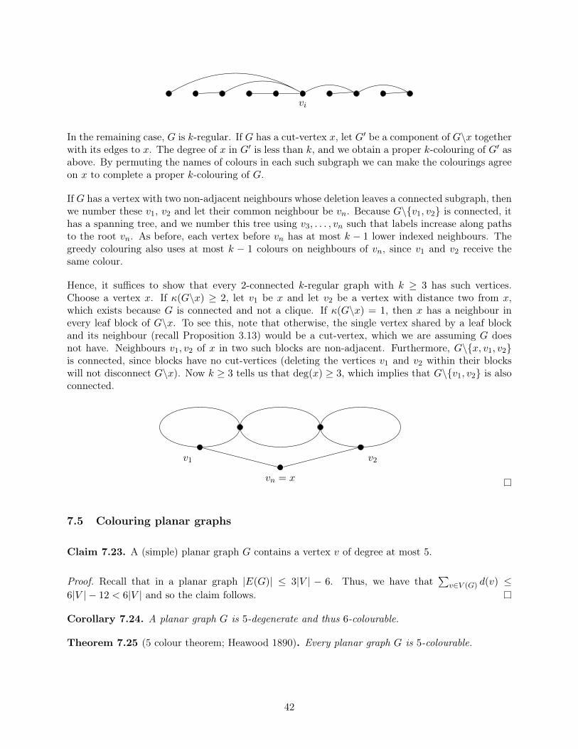
vi

In the remaining case, G is k-regular. If G has a cut-vertex x, let G′ be a component of G\x togetherwith its edges to x. The degree of x in G′ is less than k, and we obtain a proper k-colouring of G′ asabove. By permuting the names of colours in each such subgraph we can make the colourings agreeon x to complete a proper k-colouring of G.

If G has a vertex with two non-adjacent neighbours whose deletion leaves a connected subgraph, thenwe number these v1, v2 and let their common neighbour be vn. Because G\{v1, v2} is connected, ithas a spanning tree, and we number this tree using v3, . . . , vn such that labels increase along pathsto the root vn. As before, each vertex before vn has at most k − 1 lower indexed neighbours. Thegreedy colouring also uses at most k − 1 colours on neighbours of vn, since v1 and v2 receive thesame colour.

Hence, it suffices to show that every 2-connected k-regular graph with k ≥ 3 has such vertices.Choose a vertex x. If κ(G\x) ≥ 2, let v1 be x and let v2 be a vertex with distance two from x,which exists because G is connected and not a clique. If κ(G\x) = 1, then x has a neighbour inevery leaf block of G\x. To see this, note that otherwise, the single vertex shared by a leaf blockand its neighbour (recall Proposition 3.13) would be a cut-vertex, which we are assuming G doesnot have. Neighbours v1, v2 of x in two such blocks are non-adjacent. Furthermore, G\{x, v1, v2}is connected, since blocks have no cut-vertices (deleting the vertices v1 and v2 within their blockswill not disconnect G\x). Now k ≥ 3 tells us that deg(x) ≥ 3, which implies that G\{v1, v2} is alsoconnected.

vn = x

v1 v2

7.5 Colouring planar graphs

Claim 7.23. A (simple) planar graph G contains a vertex v of degree at most 5.

Proof. Recall that in a planar graph |E(G)| ≤ 3|V | − 6. Thus, we have that∑

v∈V (G) d(v) ≤6|V | − 12 < 6|V | and so the claim follows.

Corollary 7.24. A planar graph G is 5-degenerate and thus 6-colourable.

Theorem 7.25 (5 colour theorem; Heawood 1890). Every planar graph G is 5-colourable.

42

Proof. By induction of |V (G)|. For |V (G)| ≤ 5 the statement is obvious. Assume |V (G)| > 5. Let vbe a vertex of degree at most 5 in G. By induction, G\v is 5-colourable. If d(v) < 5, then a colouringof f : V (G) \ {v} → {1, . . . , 5} can be extended to V (G) by assigning f(v) ∈ {1, . . . , 5} \ {f(u) :uv ∈ E(G)}. Hence, we may assume that d(v) = 5. Fix a planar embedding of G in which theneighbours of v are coloured by f with the colours 1, . . . , 5 in clockwise order (if f uses less than5 colours on N(v) then it can be extended to V (G) as before). Let the corresponding vertices bev1, . . . , v5, i.e., f(vi) = i for i = 1, . . . , 5.

v1

v2

v3

v4

v5

For 1 ≤ i 6= j ≤ 5 let Gij be the subgraph of G\v induced by the colours i and j. Switching thetwo colours in any connected component of Gij again gives a proper 5-colouring of G\v. If thecomponent of Gij containing vi does not contain vj then we switch the colours in the componentof Gij which contains vi, in order to remove the colour i from N(v); we can then colour v with thecolour i. We can therefore assume that for every pair 1 ≤ i 6= j ≤ 5 the component of Gij containingvi also contains vj . Let Pij be a path in Gij from vi to vj . Obviously, the vertices of Pij are colouredalternatively by colours i and j. Consider paths P13 and P24. By the Jordan curve theorem (lookat the picture above!), they should intersect. Since the drawing is planar, they intersect in a vertex.But all the vertices of P13 are coloured 1 and 3 and all the vertices of P24 are coloured 2 and 4,contradiction!

Theorem 7.26 (Appel-Haken 1977; conjectured by Guthrie in 1852). Every planar graph is 4-colourable. (the countries of every plane map can be 4-coloured so that neighbouring countries getdistinct colours).

Remark 7.27. The only known proofs heavily use computers.

8 More colouring results

Theorem 8.1 (Gallai, Roy). If D is an orientation of G with longest path length `(D), then χ(G) ≤1 + `(D). Furthermore, equality holds for some orientation of G.

Proof. Suppose D is an orientation of G. Let D′ be a maximal acyclic subdigraph of D (this meansthat adding any additional edge of D to D′ would create a directed cycle). An obvious way to obtainsuch a subgraph is to start from the empty digraph on the same set of vertices, and arbitrarily add

43

edges of D one-by-one as long as these new edge do not create a directed cycle. When we cannotadd any further edges, we will have a suitable subdigraph D′.

Colour V (G) by letting f(v) be one more than the length of the longest path in D′ that ends atv. Because D′ is acyclic, for every edge u → v, the longest path in D′ ending in u cannot containv. Therefore any path ending at u can be extended to a longer path ending at v, showing thatf(v) > f(u). This shows that f strictly increases along each path in D′.

The colouring f uses colours 1 through 1 + `(D′) on V (D′) = V (G). We now prove that f is aproper colouring of G. If (u, v) ∈ E(D′), the above discussion immediately shows that f(u) 6= f(v).Otherwise, if (u, v) ∈ E(D) which is not in D′, there is a path in D′ between its endpoints (sincethe addition of (u, v) to D′ creates a cycle). This again implies f(u) 6= f(v), since f increases alongpaths of D′.

To prove the second statement, we construct an orientation D∗ such that `(D∗) ≤ χ(G)− 1. Let fbe an optimal colouring of G. For each edge (u, v) in G, orient the edge as u→ v in D∗ if and onlyif f(u) < f(v). Since f is a proper colouring, this defines an orientation. Since the labels used by fincrease along each path in D∗, and there are only χ(G) labels in f , we have `(D∗) ≤ χ(G)− 1.

8.1 Large girth and large chromatic number

The bound χ(G) ≥ ω(G) can be tight, but (surprisingly) it can also be arbitrarily bad. Thereare graphs having arbitrarily large chromatic number, even though they do not contain K3. Manyconstructions of such graphs are known, though none are trivial. We give one here.

Example 8.2 (Mycielski’s construction). Mycielski (1955) found a construction that builds fromany k-chromatic triangle-free graph G a (k+1)-chromatic triangle-free supergraph G′. Given G withvertex set V = {v1, . . . , vn}, add vertices U = {u1, . . . , un} and one more vertex w. Beginning withG′[V ] = G, add edges to make ui adjacent to all of NG(vi), and then make N(w) = U . Note that U isan independent set in G′. From the 2-chromatic graph K2, one iteration of Mycielski’s constructionyields the 3-chromatic C5, and a second iteration yields the 4-chromatic Grötzsch graph drawn below.These graphs are the triangle-free k-chromatic graphs with fewest vertices for k = 2, 3, 4.

w

Theorem 8.3. Mycielski’s construction produces a (k + 1)-chromatic triangle-free graph from ak-chromatic triangle-free graph.

Proof. Suppose G is triangle-free, χ(G) = k, V (G) = {v1, . . . , vn} and V (G′) = {vi}i∈[n]∪{ui}i∈[n]∪{w}, as described above. Since {ui}i∈[n] is independent in G′ and there are no edges from w to V (G),there is no triangle containing w. Moreover, any triangle containing ui has two other vertices inV (G) and these vertices are also neighbours of vi, which completes a triangle in G. Therefore, if Gis triangle-free, then G′ is also triangle-free.

44

A proper k-colouring f of G extends to a proper (k + 1)-colouring of G′ by setting f(ui) = f(vi)and f(w) = k + 1. Now suppose, for contradiction, that G′ has a proper k-colouring g. We mayassume that g(w) = k, which restricts g to [k − 1] on {ui}i∈[n]. Let A = {vi : g(vi) = k}. Wewill change the colouring on A to obtain a proper (k − 1) colouring of G, which is a contradictionof the fact χ(G) = k. For each vi ∈ A, we change the colour of vi to g(ui). Because g properlycolours G′, A is an independent set in G, so we need only to check edges of the form (vi, v

′) withv′ ∈ V (G)\A. If (vi, v

′) ∈ E(G), then we have constructed G′ so that (ui, v′) ∈ E(G′), which implies

g(ui) 6= g(v′). Hence our alteration does not violate the properness of the colouring on edges withinG. We ignore possible conflicts between vi and uj , because we now delete {ui}i∈[n] ∪ {w} and havea proper (k − 1)-colouring of G.

G U

w

Definition 8.4. The girth of a graph is the length of its shortest cycle.

Theorem 8.5 (Erdős, 1959). Given k ≥ 3 and g ≥ 3, there exists a graph with girth at least g andchromatic number at least k.

This result is especially surprising because if a graph has no short cycles then it “locally” looks likea tree, and all trees have chromatic number at most 2. This shows that the chromatic number reallydepends on the global structure of a graph, and cannot be estimated from local considerations.

The proof of Theorem 8.5 uses the so-called probabilistic method.

8.1.1 Digression: the probabilistic method

The general idea of the probabilistic method is to prove the existence of certain structures byshowing that they exist with positive probability in some probability space. Let us introduce someprobabilistic notation and results.

Definition 8.6. The expectation EX of a random variable X is the “average” value it takes: if Xtakes only countably many possible values, then

E[X] =∑x

xPr[X = x].

Remark 8.7. Expectation has the following properties:

• Expectation is linear: E[X + Y ] = E[X] + E[Y ], regardless of whether X and Y are indepen-dent.

45

• If X is a nonnegative integer valued random variable then

E[X] =

∞∑x=0

xPr[X = x] ≥∞∑x=1

Pr[X = x] = Pr[X ≥ 1].

In particular, if E[X] < 1 then Pr[X = 0] = 1− Pr[X ≥ 1] ≥ 1− E[X] > 0.

• More generally, for any positive a,

E[X] =∞∑x=0

xPr[X = x] ≥∑x≥a

aPr[X = x] = aPr[X ≥ a].

Dividing by a, we get Markov’s inequality : Pr[X ≥ a] ≤ E[X]/a.

Before we proceed to the proof of Theorem 8.5, let us illustrate the method on a slightly easierproblem.

A tournament is an orientation of the complete graph Kn. The name comes from observing thatsuch a digraph corresponds to an n-player round-robin tournament, where every player plays againsteveryone else exactly once, and there are no draws. An edge from a to b means that player a beatsplayer b.

Theorem 8.8. There is a tournament on n vertices where any log2 n2 vertices are beaten by some

other vertex.

Proof. Set k = log2 n2 and consider the random tournament where each edge of Kn is given a random

orientation (each direction with probability 1/2) independently from the others. For a set K of kvertices, let XK be the indicator random variable of the even that K is not beaten by any othervertex. Then Pr[XK = 1] = (1 − 1

2k)n−k. The variable X =

∑|K|=kXK counts the number of

such “bad” k-sets. Next we bound the expectation of X using the easy estimates(nk

)≤ nk and

1− x ≤ e−x:

E[X] =∑|K|=k

XK =

(n

k

)(1− 1

2k)n−k ≤ nk · e

n−k2k = exp(k log n− n− k√

n).

Here the exponent tends to −∞ and hence E[X]→ 0 as n→∞. So for n large enough, E[X] < 1.Applying the observation above, we get Pr[X = 0] > 0, i.e., the random tournament satisfies thedesired property with positive probability. This proves the existence of such a tournament.

We will look at tournaments in more depth later in the course (Section 10.2).

8.1.2 Proof of Theorem 8.5

Proof. Given a large value of n (large enough to satisfy inequalities we will use later), we randomlygenerate a graph with vertex set [n]. Simply let each pair (x, y) ∈ [n]2 be an edge with probabilityp, independently. A graph with no large independent set has large chromatic number since χ(G) ≥

46

n(G)/α(G). We therefore choose p large enough to make the existence of large independent setsunlikely. We also want to choose p small enough that the expected number of short cycles (lengthless than g) is small. When we have such a graph satisfying both conditions, we can delete a vertexfrom each short cycle to obtain the desired graph.

To make it unlikely that the graph generated will have more than n/2 short cycles, we let p = nt−1,where t = 1/(2g). Let X denote the number of cycles of length less than g in the resulting randomgraph. For each possible cycle C, define a random variable XC that takes the value 1 if C is presentin our random graph, and 0 otherwise. We then have X =

∑C XC , where the sum is over all possible

cycles C of length less than g.

Since there are at most ni potential cycles of length i, linearity of expectation yields E[X] ≤∑g−1i=3 n

ipi =∑g−1

i=3 nti < 2ntg = 2

√n. This implies that E[X]/n→ 0 as n→∞. Since E[X]/n→ 0,

we also have Pr[X ≥ n/2]→ 0 as n→∞ by Markov’s inequality. In particular, we can take n largeenough so that Pr[X ≥ n/2] < 1/2.

Since we will retain at least n/2 vertices, it suffices to show that there will be such graphs withα(G) ≤ n/(2k); α(G) cannot grow when we delete vertices, and hence at least k independent setswill be needed to cover the remaining vertices. With r = bn/(2k)c, we have

Pr[α(G) > r] ≤(

n

r + 1

)(1− p)(

r+12 ) <

(ne−pr/2

)r+1.

As n→∞ we have ne−pr/2 = ne−nt/(4k) → 0 (and r →∞), so Pr[α(G) > r]→ 0. If we also make n

large enough that Pr[X ≥ n/2] < 1/2 and Pr[α(G) > r] < 1/2, there will exist an n-vertex graph Gsuch that α(G) ≤ n/(2k) and G has fewer than n/2 cycles of length less than g. We delete a vertexfrom each short cycle and retain a graph with girth at least g and chromatic number at least k.

8.2 Chromatic number and clique minors

Definition 8.9. Let e = (x, y) be an edge of a graph G = (V,E). By G/e we denote the graphobtained from G by contracting the edge e into a new vertex ve, which becomes adjacent to allthe former neighbours of x and of y. Formally, G/e is a graph (V ′, E′) with vertex set V ′ :=(V \ {x, y}) ∪ {ve} (where ve is the ‘new’ vertex, i.e. ve /∈ V ∪ E) and edge set

E′ := {(v, w) ∈ E | {v, w} ∩ {x, y} = ∅} ∪ {(ve, w) | (x,w) ∈ E \ {e} or (y, w) ∈ E \ {e}}

x

y

e

G

ve

G/e

H is a minor of G if it can be obtained from G by deleting vertices and edges, and contractingedges.

47

Question 8.10. We know that if G has high chromatic number then it might not have a largeclique. However, must G necessarily have a subgraph which is similar to a clique?

Conjecture 8.11 (Hadwiger). If χ(G) ≥ t then G has a t-clique minor.

Note that large chromatic number implies large maximum degree.

Theorem 8.12 (Mader). If the average degree of G is at least 2t−2 then G has a Kt minor.

Proof. We proceed by induction on t+ |V (G)|. If t = 2, then the average degree of G is at least 1.This means G has an edge; this is a K2 minor.

Suppose now that d̄(G) ≥ 2t−1, i.e., e(G) ≥ 2t−2n. Let v be any vertex and let u ∈ N(v). If u andv have at most 2t−2 − 1 common neighbours, contract the edge e = (u, v). Note that the number ofvertices of G/e is one less than the number of vertices of G and that the number of edges in G/edecreased by at most (2t−2 − 1) + 1 = 2t−2 (note that when we contract e we lose the edge e, andone edge for every common neighbour of u and v). Thus,

d̄(G/e) =2e(G/e)

n− 1≥ 2(e(G)− 2t−2)

n− 1≥ 2t−1n− 2t−1

n− 1= 2t−1.

Therefore, by induction G/e has a Kt+1 minor and so G also has one. We may assume now that forevery u ∈ N(v) the vertices u and v have at least 2t−2 common neighbours. In that case it is clearthat G′ = G[N(v)] has d̄(G′) ≥ 2t−2. Thus, by induction G′ has a Kt minor which, together with v,gives a Kt+1 minor in G.

Remark 8.13. It is known that d̄(G) ≥ ct√

log t already implies the existence of a Kt minor in G,for some constant c > 0.

8.3 Edge-colourings

Definition 8.14. A k-edge-colouring of G is a labeling f : E(G) → [k]; the labels are “colours”.A proper k-edge-colouring is a k-edge-colouring such that edges sharing a vertex receive differentcolours; equivalently, each colour class is a matching. A graph G is k-edge-colourable if it has aproper k-edge-colouring. The edge-chromatic number or chromatic index χ′(G) is the minimum ksuch that G is k-edge colourable.

Remark 8.15.

(i) An edge-colouring of a graph G is the same as a vertex-colouring of its line graph L(G).

(ii) A graph G with maximum degree ∆ has χ′(G) ≥ ∆ since the edges incident to a vertex ofdegree ∆ must have different colours.

(iii) If G has maximum degree ∆ then L(G) has maximum degree at most 2(∆−1) (see the picturebelow for the basic idea of why this is true).

48

e

︸︷︷︸≤∆−1

︸︷︷︸≤∆−1

So it follows from (i) that χ′(G) ≤ 2∆− 1.

Theorem 8.16 (Kőnig 1916). If G is a bipartite multigraph, then χ′(G) = ∆(G).

Proof. An edge colouring is actually a partition of the edge set of a graph into matchings. Wetherefore make use of the theory of matchings from Section 5.

Corollary 5.9 states that every regular bipartite graph H has a perfect matching. This also holdsfor multigraphs, with the same proof. By induction on ∆(H), this yields a proper ∆(H)-edge-colouring. It therefore suffices to show that every bipartite multigraph G with maximum degree khas a k-regular bipartite supergraph H ⊃ G.

We construct such a supergraph. If G does not have the same number of vertices in each partiteset, add vertices to the smaller set to equalize the sizes. If the resulting G′ is not regular, then eachpartite set has a vertex with degree less than ∆(G′) = ∆(G). Add an edge consisting of this pair.Continue adding such edges until the graph becomes regular.

Theorem 8.17 (Vizing). Let G be a simple graph with maximum degree ∆. Then ∆(G) ≤ χ′(G) ≤∆(G) + 1.

Proof. The inequality ∆(G) ≤ χ′(G) being trivial, we show χ′(G) ≤ ∆(G) + 1. We prove this byinduction on the number of vertices of G, by applying the following claim with k = ∆ + 1 and anyvertex v.

Claim. Let v be a vertex such that v and all its neighbours have degree at most k, while at mostone neighbour has degree precisely k. Then if G\v is k-edge-colourable, G is also k-edge-colourable.

We prove the claim by induction on k. We can assume that each neighbour u of v has degree k− 1,except for one of degree k, since otherwise we can add a new vertex w and an edge (u,w) withoutviolating the conditions in the claim. We can do this until all neighbours of v have degree k − 1,except for one having degree k. Similarly we can assume v has degree k, since otherwise we canrepeatedly add new vertices adjacent only to v.

Consider any k-edge-colouring of G\v. For i = 1, . . . , k, let Xi be the set of neighbours of v that aremissed by colour i. All but one of the neighbours of v have degree k−2 in G\v (these neighbours aremissing two colors on their edges), and one neighbor of v has degree k− 1 in G\v so (this neighbourmisses one color on its edges). So all but one neighbour of v are in precisely two of the Xi, and oneneighbour is in precisely one Xi. Hence

k∑i=1

|Xi| = 2(k − 1) + 1 < 2k. (6)

49

We can assume that we have chosen the colouring such that∑k

i=1 |Xi|2 is minimized. Then for anyi, j = 1, . . . , k:

||Xi| − |Xj || ≤ 2. (7)

For if, say, |X1| > |X2| + 2, consider the subgraph H made by all edges of colours 1 and 2. Eachcomponent of H is a path or an even cycle. At least one component of H contains more verticesin X1 than in X2. This component is a path P starting in X1 and not ending in X2. Exchangingcolours 1 and 2 on P reduces X1 by two and increases X2 by two. This reduces |X1|2 + |X2|2,contradicting our minimality assumption. This proves (7).

It follows that there exists an i with |Xi| = 1, since otherwise by (6) and (7) each |Xi| is 0 or 2,while their sum is odd, a contradiction.

So we can assume |Xk| = 1, say Xk := {u}. Let G′ be the graph obtained from G by deleting theedge (v, u) and deleting all edges of colour k. So G′\v is (k − 1)-edge-coloured. Moreover, in G′,vertex v and all its neighbours have degree at most k − 1, and at most one neighbour has degreek− 1. So by the induction hypothesis, G′ is (k− 1)-edge-colourable. Restoring colour k, and givingedge (v, u) colour k, gives a k-edge-colouring of G. (Giving (v, u) colour k does not violate theproperness of the colouring: v has no other adjacent edges coloured k by construction, and sinceu ∈ Xk, u also has no other adjacent edges coloured k).

Remark 8.18. In general it is a hard problem to decide whether χ′(G) = ∆(G).

8.4 List colouring

List colouring is a more general version of the usual colouring problem. We still want to pick a singlecolour for each vertex, but the set of colours available at each vertex may be restricted.

Definition 8.19. For each vertex v in a graph G, let L(v) denote a list of colours available for v. Alist colouring or choice function from a given collection of lists is a proper colouring f such that f(v)is chosen from L(v). A graph G is k-choosable or k-list-colourable if it has a proper list colouringfrom every assignment of k-element lists to the vertices. The list chromatic number or choosabilityχl(G) is the minimum k such that G is k-choosable.

Since the lists can be chosen to be identical, χl(G) ≥ χ(G). If the lists have size at least 1 + ∆(G),then colouring the vertices in succession leaves an available colour at each vertex. This argument isanalogous to the greedy colouring algorithm and proves that χl(G) ≤ ∆(G) + 1. It is not possible,however, to place an upper bound on χl(G) in terms of χ(G). For example, there are bipartitegraphs with arbitrarily large list-chromatic number.

Theorem 8.20 (Erdős, Rubin, Taylor 1979). If m =(

2k−1k

), then Km,m is not k-choosable.

Proof. Let X,Y be the bipartition of G = Km,m. For each of X and Y , let the lists of the verticesbe all the k-subsets of [2k − 1]. Suppose G has a choice function f . If f uses fewer than k distinctchoices in X, then there is a k-set K ⊂ [2k − 1] not used, which means that no colour was chosenfor the vertex of X having K as its list. If f uses at least k colours on vertices of X, then there isa k-set K ⊂ [2k − 1] of colours used in X, and no colour can be properly chosen for the vertex Ywith list K.

50

Definition 8.21. Let L(e) denote the list of colours available for e. A list edge-colouring is a properedge-colouring f with f(e) chosen from L(e) for each e. The list chromatic index or edge-choosabilityχ′l(G) is the minimum k such that G has a proper list edge-colouring for each assignment of lists ofsize k to the edges. Equivalently, χ′l(G) = χl(L(G)), where L(G) is the line graph of G.

Conjecture 8.22. χ′l(G) = χ′(G), and in particular χ′l(G) ≤ ∆(G) + 1.

Theorem 8.23 (Galvin,1995). χ′l(Kn,n) = n.

Note that the graph L(Kn,n) is essentially an n × n grid. That is, the vertices of L(Kn,n) can bearranged in an n × n grid, where vertices are adjacent if and only if they share a row or share acolumn. (This graph is known as the Cartesian product Kn ×Kn). Theorem 8.23 therefore has thefollowing appealing equivalent formulation. If we have an n×n grid where each cell is assigned a listof n colours, then we can choose a colour for each cell such that each row and column have distinctcolours.

Definition 8.24. A kernel of a digraph is an independent set S having an edge to every vertexoutside S. A digraph is kernel-perfect if every induced sub-digraph has a kernel. Given a functionf : V (G)→ N, the graph G is f-choosable if a proper list colouring can be chosen whenever the listssatisfy |L(x)| ≥ f(x) for each x.

Lemma 8.25. If D is a kernel-perfect orientation of G and f(x) = d−D(x) for all x ∈ V (G), thenG is (1 + f)-choosable.

Proof. By induction on |G|; trivial for |G| = 1. Suppose |G| > 1, and consider an assignment oflists, with the list L(x) for each x having size 1+f(x). Choose a colour c appearing in some list. LetU = {v : c ∈ L(v)}. Let S be the kernel of the induced subdigraph D[U ]. Assign the colour c to allof S, which is permissible since S is independent. Delete c from L(v) for each v ∈ U\S. Althoughthe list of every vertex in U\S lost color c, the indegree of these vertices in D\S also decreased byat least one. Hence we still have at least d−D\S(u) + 1 colors left in the list for every vertex in U\S.Therefore for each x ∈ V (D)\S its list has size at least 1 + f ′(x) , where f ′(x) = d−D\S(x). By theinduction hypothesis, D\S is (1 + f ′)-choosable, so we can complete a list colouring for the originalgraph from the remaining colours at V (G)\S.

Proof of Theorem 8.23. First note that χ′l(Kn,n) ≥ χ′(Kn,n) ≥ n.

It suffices by the lemma to prove that D = Kn × Kn has a kernel-perfect orientation with eachvertex having indegree and outdegree n− 1. Label the vertices with labels 1, 2, . . . , n so that vertex(r, s) has label r + s − 1 modn. Note that the labels of vertices in every row and column are justpermutations of {1, . . . , n}. Define an orientation of Kn ×Kn by directing edges from vertex (r, s)to the vertices in row r with higher labels and to the the vertices in column s with lower labels.Since label j is higher than j− 1 other labels, a vertex with label j has j− 1 predecessors in its rowand n− j predecessors in its column. Hence each vertex has indegree n− 1 and outdegree n− 1.

1 2 3 · · · n

2 3. . . n 1

3. . . . . . . . .

...... n

. . . . . . n− 2n 1 · · · n− 2 n− 1

51

We prove that for every set of vertices U ⊆ D, the subdigraph D[U ] has a kernel, by induction on|U |. The case |U | = 1 is trivial, because U itself is trivially an independent set. Otherwise, considerthe set S0 consisting of the vertices which have minimum label in their row (among the vertices inU). This means that each u ∈ S0 has no incoming arcs from vertices of U , in its row. If no twovertices of S0 fall in the same column then S0 is an independent set, therefore a kernel. Otherwise,there is a column C with multiple vertices of S0. Let u be the vertex of S0 with the minimum labelin C. Then D[U\u] has a kernel S by induction. S must contain a vertex from C, because the non-uvertices in C ∩S0 must have incoming arcs from S, and these incoming arcs cannot come from theirrows. By the choice of u, any such vertex in C has an edge to u, so we conclude that S has an edgeto every vertex in U , and is a kernel, as required.

9 The Matrix Tree Theorem

In Section 2.3 we gave two proofs of the following classical result.

Theorem 9.1 (Cayley’s formula). There are nn−2 labeled trees on n vertices.

Here we will show yet another proof that we deduce from a very general theorem about countingspanning trees in graphs. Indeed, we can think of the number of labeled trees as the number ofspanning trees in the complete graph Kn.

Now consider an arbitrary connected simple graph G on vertex set [n], and denote the numberof spanning trees by t(G). The following celebrated result is Kirchhoff’s matrix tree theorem. Toformulate it, consider the incidence matrix B of G (as in Definition 1.13), and replace one of thetwo 1’s by −1 in an arbitrary manner to obtain the matrix C (we say C is the incidence matrix ofan orientation of G). M = CCT is then a symmetric n× n matrix, which isd(1) · · · 0

.... . .

...0 · · · d(n)

−AG.Theorem 9.2 (Matrix tree theorem). We have t(G) = detMii for all i = 1, . . . , n, where Mii resultsfrom M by deleting the i-th row and the i-th column.

The key to the proof is the following theorem of Binet and Cauchy:

Theorem 9.3. If P is an r × s matrix and Q is an s× r matrix with r ≤ s, then

det(PQ) =∑Z

(detPZ)(detQZ),

where PZ is the r × r submatrix of P with column set Z, and QZ is the r × r submatrix of Q withthe corresponding rows Z, and the sum is over all r-sets Z ⊆ [s].

We will prove Theorem 9.3 in the next section (Section 9.1), but for now we use it to give the proofof Theorem 9.2.

52

Proof of Theorem 9.2. Note that C has at least n− 1 columns, because the connected graph G hasat least n− 1 edges. This means that we can apply Theorem 9.3 to Mii and get

detMii =∑N

detN · detNT =∑N

(detN)2,

where N runs through all (n − 1) × (n − 1) submatrices of C \ {row i}. The n − 1 columns of Ncorrespond to a subgraph of G with n− 1 edges on n vertices, and it remains to show that

detN =

{±1 if these edges span a tree0 otherwise.

Suppose the n−1 edges do not span a tree. Then there exists a component that does not contain thevertex i. Since the corresponding rows of this component add to 0, we infer that they are linearlydependent, and hence detN = 0.

Assume now that the columns of N span a tree. Then there is a vertex j1 6= i of degree 1; let e1

be the incident edge. Deleting j1, e1 we obtain a tree with n − 2 edges. Again there is a vertexj2 6= i of degree 1 with incident edge e2. Continue in this way until j1, . . . , jn−1 and e1, . . . , en−1

with ji ∈ ei are determined. Now permute the rows and columns to bring jk into the k’th row andek into the k’th column. Since by construction jk 6∈ el for k < l, we see that the new matrix N ′ islower triangular with all elements on the main diagonal equal to ±1. Thus detN = ±detN ′ = ±1,and we are done.

Third proof of Cayley’s formula. In the special case G = Kn, we have

M =

n− 1 −1 · · · −1−1 n− 1 −1...

. . ....

−1 −1 · · · n− 1

.(The (n− 1)s on the diagonal correspond to the fact that the degree of each vertex is n− 1, and the−1s in the other positions i, j correspond to the fact that there is an edge between each i and j).

The (n− 1) × (n− 1) matrices Mii have the same form as M . To compute detMii, add all thecolumns to the first column to get

detMii = det

1 −1 · · · −11 n− 1 −1...

. . ....

1 −1 · · · n− 1

,then add the first column to all the rest to get

detMii = det

1 0 · · · 01 n 0...

. . ....

1 0 · · · n

.

53

This is a lower-triangular matrix, so we can see detMii = nn−2. Then Theorem 9.2 finishes theproof.

9.1 Lattice paths and determinants

In this section we will introduce some theory connecting graphs and determinants. In particular wewill establish the Cauchy-Binet Theorem (Theorem 9.3).

The starting point of our discussion is the usual permutation representation of the determinant of amatrix. Let M = (mij) be a real n× n matrix. Then

detM =∑σ

sign(σ)m1σ(1)m2σ(2) · · ·mnσ(n), (8)

where σ runs through all permutations of [n], and the sign of σ is 1 or −1, depending on whether σis the product of an even or an odd number of transpositions.

Now we pass to graphs, more precisely to weighted directed bipartite graphs. Let the verticesa1, . . . , an stand for the rows of M , and b1, . . . , bn for the columns. For each pair i, j, draw anarrow from ai to bj and give it the weight mij , as in the figure.

a1 · · · ai · · · an

b1 · · · bj · · · bn

m11

mi1 mij

mnjmnn

In terms of this graph, the formula (8) has the following interpretation:

• The left-hand side is the determinant of the path matrix M , whose (i, j) entry is the weight ofthe (unique) directed path from ai to bj .

• The right-hand side is the weighted (signed) sum over all vertex-disjoint path systems fromA = {a1, . . . , an} to B = {b1, . . . , bn}. Such a system Pσ is given by paths

a1 → bσ(1), . . . , an → bσ(n),

and the weight of the path system Pσ is the product of the weights of the individual paths:

w(Pσ) = w(a1 → bσ(1)) · · ·w(an → bσ(n)).

In this interpretation formula (8) reads

detM =∑σ

sign(σ)w(Pσ).

A natural generalization of (8) from bipartite to arbitrary graphs was found by Gessel and Viennot.This widely applicable result has a very simple and elegant proof, as we will see below.

54

Let us first collect the necessary concepts. We are given a finite acyclic directed graph G = (V,E),i.e. one that has no directed cycles in it. In particular, there are only finitely many directed pathsbetween any two vertices a and b in G, where we include all trivial paths a→ a of length 0. Everyedge e carries a weight w(e). If P is a directed path from a to b, written shortly P : a→ b, then wedefine the weight of P as

w(P ) =∏e∈P

w(e),

which is defined to be 1 if P is a path of length 0.

Now let A = {a1, . . . , an} and B = {b1, . . . , bn} be two sets of n vertices, where A and B are notnecessarily disjoint. To A and B we associate the path matrix M = (mij) with

mij =∑

P :ai→bj

w(P ).

A path system P from A to B consists of a permutation σ together with n paths Pi : ai → bσ(i) fori = 1, . . . , n. We write sign(P) = sign(σ). The weight of P is the product of the path weights

w(P) =n∏i=1

w(Pi), (9)

which is the product of the weights of all the edges of the path system.

Finally, we say that the path system P = (P1, . . . , Pn) is vertex-disjoint if the paths of P are pairwisevertex-disjoint.

Lemma 9.4 (Gessel-Viennot). Let G = (V,E) be a finite weighted acyclic directed graph, A ={a1, . . . , an} and B = {b1, . . . , bn} two n-sets of vertices, and M the path matrix from A to B. Then

detM =∑

P vertex−disjointpath system

sign(P)w(P). (10)

Proof. A typical summand of det(M) is sign(σ)m1σ(1) · · ·mnσ(n), which can be written as

sign(σ)

∑P1:a1→bσ(1)

w(P1)

· · · ∑Pn:an→bσ(n)

w(Pn).

Summing over σ we immediately find from (9) that

detM =∑P

sign(P)w(P),

where P runs through all path systems from A to B (vertex-disjoint or not). Hence to arrive at(10), all we have to show is ∑

P∈Nsign(P)w(P) = 0, (11)

55

where N is the set of all path systems that are not vertex-disjoint. To show this, we exhibit aninvolution π : N → N (without fixed points) such that for P and πP

w(πP) = w(P) and sign(πP) = − sign(P).

This will clearly imply (11) and thus the formula (10) of the Lemma.

The involution π is defined in a natural way. Let P ∈ N with paths Pi : ai → bσ(i). By definition,some pair of paths will intersect:

ai0 aj0

bσ(j0)bσ(i0)

X

• Let i0 be the minimal index such that Pi0 shares some vertex with another path.

• Let x be the first such common vertex on the path Pi0 .

• Let j0 be the minimal index (j0 > i0) such that Pj0 has the vertex x in common with Pi0 .

Now we construct the new system πP = (P ′1, . . . , P′n) as follows:

• Set P ′k = Pk for all k 6= i0, j0.

• The new path P ′i0 goes from ai0 to x along Pi0 , and then continues to bσ(j0) along Pj0 . Similarly,P ′j0 goes from aj0 to x along Pj0 and continues to bσ(i0) along Pi0 .

Clearly π(πP) = P, since the index i0, the vertex x and the index j0 are the same as before. In otherwords, applying π twice we switch back to the old paths Pi. Next, since πP and P use preciselythe same edges, we certainly have w(πP) = w(P). And finally, since the new permutation σ′ isobtained by multiplying σ with the transposition (i0, j0), we find that sign(πP) = − sign(P), andwe are done.

The Gessel-Viennot Lemma can be used to derive basic properties of determinants, just by lookingat appropriate graphs. For us, it will serve as a tool to deduce the Cauchy-Binet formula.

Proof of Theorem 9.3. As before, let A and B be vertex sets corresponding to the rows and columns,respectively, of the matrix P . Similarly let B and C correspond to the matrix Q. Consider now

56

the concatenated graph as indicated in the figure, and observe that the (i, j)-entry mij of the pathmatrix M from A to C is precisely mij =

∑k pikqkj , thus M = PQ.

Te vertex-disjoint path systems from A to C in the concatenated graph correspond to pairs ofsystems from A to Z and Z to C, for r-element subsets Z of B. The result follows immediatelyfrom Lemma 9.4, by noting that sign(στ) = sign(σ) sign(τ).

a1 · · · ai · · · ar

b1 · · · bk · · · bs

c1 · · · cj · · · cr

pi1 pik

qij qkj

10 More Theorems on Hamiltonicity

Definition 10.1. The (Hamiltonian) closure of a graph G, denoted C(G), is the subgraph of G onV (G) obtained by iteratively adding edges between pairs of nonadjacent vertices whose degree sumis at least n, until no such pair remains. In the example below, n = 6.

→ → →

Theorem 10.2 (Bondy Chvátal 1976). A simple n-vertex graph is Hamiltonian if and only if itsclosure is Hamiltonian.

Sketch of Proof. Suppose G∪ {(u, v)} is Hamiltonian and d(u) + d(v) ≥ n. Then G has a Hamiltonpath from u to v. Since |N(u)|+ |N(v)| ≥ n, on the path there is a vertex vi ∼ v such that the nextvertex vi+1 ∼ u (as in the proof of Dirac’s Theorem). This gives a Hamilton cycle in G.

u vi vi+1 v

Theorem 10.3 (Chvátal 1972). Suppose G has vertex degrees d1 ≤ · · · ≤ dn. If i < n/2 impliesthat di > i or dn−i ≥ n− i, then G is Hamiltonian.

57

Proof. Because adding edges to form the closure reduces no entry in the degree sequence, and agraph is Hamiltonian if and only if its closure is Hamiltonian, it suffices to consider the specialcase where G is closed. In this case, we prove that the condition implies G = Kn. We prove thecontrapositive; if G = C(G) 6= Kn, then we construct a value of i less than n/2 for which Chvátal’scondition is violated. Here violation means that at least i vertices have degree at most i and at leastn− i vertices have degree less than n− i, implying that di ≤ i and dn−i < n− i.

If G 6= Kn, then among the pairs of nonadjacent vertices we choose a pair u, v with maximum degreesum. Because G is closed, u � v implies d(u) + d(v) < n, and we may assume d(u) ≤ d(v). We thenhave d(u) < n/2; let i = d(u).

Because we chose a nonadjacent pair with maximum degree sum, every vertex of V \v that is notadjacent to v has degree at most d(u) = i; furthermore, there are at least n − 1 − d(v) ≥ d(u) = iof these vertices. Similarly, every vertex of V \u that is not adjacent to u has degree at mostd(v) < n− d(u) = n− i, and there are n− 1− d(u) = n− 1− i of these. Since d(u) ≤ d(v), we canalso add u to the set of vertices with degree at most d(v), so we obtain n − i vertices with degreeless than n − i. Hence we have proved di ≤ i and dn−i < n − i for this specially chosen i, whichcontradicts the hypothesis.

Theorem 10.4 (Chvátal-Erdős 1972). If κ(G) ≥ α(G), then G has a Hamiltonian cycle (unlessG = K2).

Proof. The theorem is trivially true for complete graphs. Otherwise, the condition requires κ(G) ≥α(G) > 1. We will prove that if G has no Hamilton cycle, then k = κ(G) < α(G). Let C be alongest cycle (which we are assuming is not Hamiltonian) in G. LetH be a component of G\C. Sinceδ(G) ≥ κ(G) and every graph with δ(G) ≥ 2 has a cycle of length at least δ + 1 (Proposition 1.32),C has at least k + 1 vertices. Also C has at least k vertices with edges to H, else the vertices of Cwith edges to H contradict κ(G) = k. Let u1, . . . , u` be the vertices of C with edges to H (` ≥ k),in clockwise order. For i = 1, . . . , k, let ai be the vertex immediately following ui on C. If any twoof these vertices are adjacent, say ai ∼ aj , then we construct a longer cycle by using (ai, aj), theportions of C from ai to uj and aj to ui, and a ui, uj-path through H (see first illustration). Thisargument includes the case ai = ui+1 (see second illustration), so we also conclude that no ai hasa neighbour in H. Hence {a1, . . . , ak} plus a vertex of H forms an independent set of size k + 1,proving that α(G) > k as desired.

aiui

ajuj

H

ai = ui+1ui

H

58

10.1 Pósa’s Lemma

Let P be a path in a graph G, say from u to v. Given a vertex x ∈ P , we write x− for the vertexpreceding x on P , and x+ for the vertex following x on P (whenever these exist). Similarly, forX ⊆ V (P ) we put

X− :={x− : x ∈ X

}and X+ :=

{x+ : x ∈ X

}.

If x ∈ P\u is a neighbour of u in G, then P ∪ {(u, x)}\{(x, x−)} (which is a path in G with vertexset V (P )) is said to have been obtained from P by a rotation fixing v (see figure below). A pathobtained from P by a (possibly empty) sequence of rotations fixing v is a path derived from P . Theset of starting vertices of paths derived from P , including u, will be denoted by S(P ). As all pathsderived from P have the same vertex set as P , we have S(P ) ⊆ V (P ).

u x− x v

P

Remark 10.5. If some sequence of rotations can delete the edge (x, x−), call this edge a brokenedge. Note that every interval of the original path not containing broken edges is traversed by allderived paths as a whole piece (however, the direction can change).

Definition 10.6. For a graph G and a subset S ⊆ V (G), let ∂S = {v ∈ G\S : ∃y ∈ S, v ∼ y}.

Lemma 10.7. Let G be a graph, let P = u . . . v be a longest path in G, and put S := S(P ). Then∂S ⊆ S− ∪ S+.

Proof. Let x ∈ S and y ∈ N(x) be given; we show that y ∈ S− ∪ S ∪ S+. As x ∈ S there is apath Q = x . . . v derived from P . Then y ∈ V (Q) = V (P ), because Q (like P ) is a longest path andcannot be extended. Let z denote the predecessor of y on Q.

Suppose that y /∈ S− ∪ S ∪ S+. Then each of the (one or two) edges e ∈ P at y lies on every pathderived from P (and in particular on Q), because in any rotation in which e is first deleted, its twoends (including y) would have become members of S and of S− ∪ S+. Hence z ∈ {y−, y+}. ButQ ∪ {(x, y)}\{(y, z)} is obtained from Q by a rotation, which puts z in S and y in S− ∪ S+.

Lemma 10.8. Let G be a graph, let P = u . . . v be a longest path in G, and put S := S(P ). Ifdeg(u) ≥ 2 then G has a cycle containing S ∪ ∂S.

Proof. Let y be the last vertex of P in ∂S. Then all the vertices from S ∪ ∂S lie on the subpathP1 of P between u and y, because any vertex in S which is after y in P would differ from v andhence have its successor on P in ∂S. Let x ∈ S be a neighbour of y in G, and let Q = x . . . v bederived from P . As in the proof of Lemma 10.7, all the edges of P after y are still edges of Q, sothe segments of Q and P after y are the same (denote this common path segment by P2 = Q2). LetQ1 be the subpath of Q between x and y. We have

S ∪ ∂S ⊆ V (P1) = V (P\P2) = V (P )\V (P2) = V (Q)\V (Q2) = V (Q1).

and Q1 ∪ {(y, x)} is a cycle in G. For this argument it is important that Q1 contains a vertex otherthan x and y. Indeed, since deg(u) ≥ 2 there is a nontrivial rotation so |S| > 1 and |Q1| = |P1| >3.

59

Corollary 10.9. Fix k ≥ 2 and let G be a graph such that for all S ⊆ V (G) with |S| ≤ k, we have|∂S| ≥ 2|S|. Then G has a cycle of length at least 3k.

Proof. Let S = S(P ) be the set of potential starting points of paths derived from a longest pathP = u . . . v. Note that every vertex of G has degree at least 2 (for a singleton set S we have|∂S| ≥ 2|S|).

If |S| < k then because u has no predecessor, we have |S− ∪ S+| < 2|S| ≤ |∂S| and therefore∂S 6⊆ S− ∪ S+. This is a contradiction of Lemma 10.7, and shows that |S| ≥ k. By Lemma 10.8, Ghas a cycle containing S ∪ ∂S. Since S has a subset of size k, we have |S ∪ ∂S| ≥ 3k.

10.2 Tournaments

Definition 10.10. A tournament is a directed graph obtained by assigning a direction to everyedge of the complete graph. That is, it is an orientation of Kn.

In the context of tournaments, it only makes sense to consider directed paths and cycles, becauseevery edge is present. So, a Hamilton cycle is a spanning directed cycle.

Theorem 10.11. Every tournament has a Hamilton path.

Proof. We proceed by induction on n. The case n = 2 is clear (there is only one tournament on twovertices, namely a single directed edge, which is already a Hamilton path).

Suppose the claim holds for all tournaments on n vertices, and let T have n + 1 vertices. Let v beany vertex of T . Then T\v is also a tournament and hence has a Hamilton path u1 → · · · → un.Note that if v → u1, we are done. So suppose u1 → v. Let i be the maximum index such thatui → v. If i = n we are done, with the Hamilton path u1 → · · · → un → v. If not then v → ui+1

and we can take the Hamilton path u1 → · · · → ui → v → ui+1 → · · · → un.

u1 u2 ui ui+1 un

v

Definition 10.12. A tournament is strongly connected if for all u, v there is a directed path from uto v.

Theorem 10.13. A tournament T is strongly connected if and only if it has a Hamilton cycle.

Proof. If T is Hamiltonian, then it is immediately clear that it is strongly connected: for any u andv simply consider the portion of a Hamilton path between u and v.

Now, suppose T is not Hamiltonian. Let C be a longest cycle in T and let v /∈ C. If C has 2consecutive vertices u, u+ such that u→ v and v → u′, then there is a longer cycle on the vertex setC ∪ {v}:

60

uu+ v

C

Otherwise all edges between v and C go in only one direction, and we can assume this holds for allv /∈ C. Let A be the set of v /∈ C such that edges go from v to C, and let B be the set of v /∈ C suchthat edges go from C to v. If one of A or B are empty, it immediately follows that T is not stronglyconnected: if say B is empty then there is no path from any vertex of C to any vertex of A.

So, suppose both of A and B are nonempty. There is no edge oriented from a vertex b ∈ B to avertex a ∈ A, because if there was we could extend C, contradicting maximality (we could replaceany edge x→ y in C with the path x→ b→ a→ y). But then there is no path from any vertex inB to any vertex in A, so again T is not strongly connected.

C

A B

11 Kuratowski’s Theorem

In Corollary 6.16 we saw that K5 and K3,3 are not planar. In this section we will prove a remarkabletheorem of Kuratowski, roughly saying that K5 and K3,3 are in some sense the only obstructions tobeing planar. We will also simultaneously prove Fáry’s theorem, that any planar graph can in factbe drawn using only straight lines.

Definition 11.1. A subdivision of a graph H is a graph obtained from H by replacing the edges ofH by internally vertex disjoint paths of non-zero length with the same endpoints.

Example 11.2.

H Subdivision of H

Remark 11.3. If G contains a subdivision of H, it also contains an H-minor.

Definition 11.4. A Kuratowski graph is a graph which is a subdivision of K5 or K3,3. If G is agraph and H is a subgraph of G which is a Kuratowski graph then we say that H is a Kuratowskisubgraph of G.

61

Theorem 11.5 (Kuratowski 1930). A graph is planar if and only if it has no Kuratowski subgraph.

It is straightforwardly true that no Kuratowski graph is planar. Indeed, given a planar drawing(by polygonal curves) of a Kuratowski subgraph, we can consider the subdivided paths to be longpolygonal curves in a planar drawing of K5 or K3,3, which is impossible. So, to prove Theorem 11.5we need only prove that every graph with no Kuratowski subgraph has a plane drawing. As promised,we prove a stronger theorem, combining Kuratowski’s Theorem with Fáry’s Theorem on straightlinedrawings.

Definition 11.6. A straightline drawing of a planar graph G is a drawing in which every edge is astraight line.

Theorem 11.7. If G is a graph with no Kuratowski subgraph then G has a straightline drawing inthe plane.

The proof of Theorem 11.7 is broken down into two parts. In the first part, we prove a version ofthe theorem for 3-connected graphs, then in the second part we show how the general case can bereduced to the 3-connected case.

11.1 Convex drawings of 3-connected graphs

Definition 11.8. A convex drawing of G is a straightline drawing in which every non-outer faceof G is a convex polygon, and the outer face is the complement of a convex polygon. (That is, theboundary of each face is the boundary of a convex polygon).

Theorem 11.9 (Tutte 1960). If G is a 3-connected graph which has no Kuratowski subgraphs thenG has a convex drawing in the plane with no three vertices on a line.

We will need some lemmas to prove Theorem 11.9.

Lemma 11.10 (Thomassen 1980). Every 3-connected graph G with at least five vertices has an edgee such that G/e is 3-connected.

Proof. We proceed by contradiction. Suppose G has no edge whose contraction yields a 3-connectedgraph. For every edge (x, y) ∈ E(G), the graph G is 3-connected but G/(x, y) is not 3-connected.A minimal (2 vertex) separating set in G/(x, y) must therefore contain the newly contracted vertex,so there exists a vertex z ∈ V (G) \ {x, y} such that {x, y, z} is a separating set in G. We call sucha vertex z a mate of the edge (x, y).

Choose an edge (x, y) ∈ E(G) and a mate z and a connected component H in G\{x, y, z}, in sucha way that H has maximum possible size. Let H ′ be another connected component of G\{x, y, z}.Since {x, y, z} is a separating set of minimal size, each of x, y and z have a neighbour in both of Hand H ′. Let u be a neighbour of z in H ′ and let v be a mate of the edge (u, z).

We claim now that the induced subgraph F of G with vertex set V (H) ∪ {x, y} \ v is connected. Ifthat is the case then we reach a contradiction because |F | > |H| and F is a connected subgraph ofG\{u, v, z}.

To prove the claim, we consider two cases: v /∈ V (H) or v ∈ V (H). The first case is straightforward:since H is connected and since x and y each have a neighbour in H, the graph F must also beconnected. Consider now the second case. The following picture gives an illustration of the situation.

62

v

x

y

zu

HH ′

Observe that G\{v, z} is connected since G is 3-connected. Thus, for any vertex w ∈ V (H) \ {v, z}there exists a path in G\{v, z} from w to {x, y}. If we can find such a path for any w ∈ V (H) \ {v}inside of F then it follows that F is connected.

We claim that we can just choose these paths to be the shortest paths (in G\{v, z}) from each wto {x, y}. Indeed, since {x, y, z} was the separating set with which we defined H, any path from wavoiding z must pass through x or y before it leaves H.

Lemma 11.11. If G has no Kuratowski subgraphs, then G/e has no Kuratowski subgraph, for anyedge e ∈ E(G).

Proof. We prove the contrapositive: if G/e contains a Kuratowski subgraph then so does G.

Let z be the vertex of G/e obtained by contracting e = (x, y). Let H be a Kuratowski subgraph inG/e. If z /∈ V (H) then it is clear that H is also a subgraph of G. Otherwise, write NH(z) = A∪B,where the vertices in A were adjacent to x while the vertices in B were adjacent to y, before thecontraction.

If |A| = 0 (respectively, |B| = 0) then we obtain a copy of H in G by replacing z with x (respectivelyy), in the copy of H in G/e. If |A| = 1 (respectively |B| = 1) we can replace z with y, add x andinclude the edge (x, y) and the edge from x to A, to obtain a copy of H with one of its edgesubdivided (specifically, the edge from z to A, respectively from z to B).

Since H is a subdivision of K3,3 or K5, every vertex has degree 2,3 or 4. The only possibility thatwe have not accounted for is that dH(z) = |NH(z)| = 4, and |A| = |B| = 2. We can then obtain asubdivision of K3,3 in G from H by replacing z with the edge (x, y) and deleting the inner verticesof two of the paths in H. This is illustrated below; the thicker lines indicate subdivided paths, andthe four vertices directly above z are in A, A, B and B respectively.

z

x y

Proof of Theorem 11.9. Let G be a 3-connected graph which has no Kuratowski subgraphs. Weprove that G has a convex drawing in the plane with no three vertices on a line, by induction on|G|.

63

The base case is |G| = 4. In that case, since G is 3-connected, the only possibility is that G = K4

and it is easy to find a suitable drawing (see for example Example 6.2).

Consider now |G| ≥ 5. The induction hypothesis says that every 3-connected graph on at most|G| − 1 vertices without Kuratowski subgraphs has a convex drawing in the plane with no threevertices on a line.

By Lemma 11.10 there exists an edge e = (x, y) ∈ E(G) such that G/e is 3-connected. Moreover,by Lemma 11.11 G/e does not have any Kuratowski subgraphs. From the induction hypothesis itfollows that G/e has a convex drawing in the plane with no three vertices on a line. Fix such aconvex drawing and let z be the vertex of G/e obtained by contracting the edge e in G. Note that ifwe delete z from G/e we get a graph which is 2-connected and hence its faces are cycles. Let C bethe cycle formed by the boundary of the face of (G/e)\z which contains z (this could be the outerface).

Observe that all the neighbours of z in G/e (and thus, also of x and y in G) lie in C. Moreover, sinceG is 3-connected, x and y each have at least 2 neighbours in C. Let z1, . . . , zk be the neighbours of zin G/e ordered cyclically (according to an orientation of C) and let zi1 , . . . , zi` denote the neighboursof x in G (in the same order). If the neighbours of y all fall in between two neighbours of x (that is,all are in {zij , zij+1, . . . , zij+1} for some j ∈ {1, . . . , `}) then we can obtain a convex drawing of Gwith no three vertices on a line by putting x at z and putting y at a point close to z in the wedgeformed by

(x, zij

)and

(x, zij+1

). Note that it is possible for the angle between

(x, zij

)and

(x, zij+1

)to be a reflex angle, as illustrated below (the vertices marked ⊗ correspond to neighbours of y). Inthis case we need to put our point in the region formed by continuing the lines zij , z and zij+1 , z,shaded in the picture below. This is so that we can draw the triangles x, y, zij and x, y, zij withoutintersecting existing lines, if necessary.

zi1

zi2⊗⊗

⊗

z x

y

In general, the reason it is always possible to choose an appropriate position for y very close to z isthat if we take a convex polygon with no three points on a line, and we perturb one of the verticesslightly, then the result is still a convex polygon. Note also that it is always possible to choose ournew point such that still no three vertices are on a line, because the set of bad positions has measurezero.

We claim the neighbours of y are always situated in between two neighbours of x, so the aboveargument is always valid. Indeed, otherwise, one of the following two cases holds:

• y shares three neighbours zj1 , zj2 and zj3 with x. In this case, the cycle C together with (x, y)and the edges from {x, y} to {zj1 , zj2 , zj3} forms a subdivision of K5 in G (left image below).

64

• y has neighbours zj1 and zj3 which alternate with two neighbours zj2 and zj4 of x in the cycleC. In that case, the cycle C together with (x, y), (x, zj2), (x, zj4), (y, zj1) and (y, zj3) forms asubdivision of K3,3 in G (right image below):

xy

xy

Since G has no Kuratowski subgraph, both of these cases are impossible.

11.2 Reducing the general case to the 3-connected case

Definition 11.12. Given a subdivision H ′ of H, we call the vertices of the original graph branchvertices.

Example 11.13. In the following picture, the branch vertices are marked with an ⊗.

H

⊗

⊗ ⊗

⊗

H ′

Fact. We make three observations. See the picture below.

1. In a Kuratowski subgraph, there are three internally vertex-disjoint paths connecting any twobranch vertices. For K5-subdivisions, we even have four such paths.

2. In a Kuratowski subgraph, there are four internally vertex-disjoint paths between any two pairsof branch vertices.

3. Any cycle in a subdivision contains at least three branch vertices.

⊗ ⊗ ⊗

⊗

Proposition 11.14. Let G be a graph with at least 4 vertices which has no Kuratowski subgraph, andsuppose that adding an edge joining any pair of non-adjacent vertices creates a Kuratowski subgraph.Then G is 3-connected.

65

Theorem 11.7 is a corollary of Proposition 11.14, as follows.

Proof of Theorem 11.7. Start with a graph G which has no Kuratowski subgraph, and add edgesas long as possible without creating a Kuratowski subgraph. Let the final graph be G′ ⊇ G. ThenG′ is 3-connected so by Theorem 11.9 it has a planar convex drawing. Therefore G has a planarstraightline drawing.

Proof of Proposition 11.14. The proof is by induction on |G|. If |G| = 4 then G is complete so weare done. So assume |G| ≥ 5.

First, note that G is connected. Otherwise, we could add an edge between connected components,and this cannot create a Kuratowski subgraph because Kuratowski graphs have no bridges.

Next, we prove that G is 2-connected. Suppose otherwise, that we can write G = G1 ∪G2 in such away that G1∩G2 = v for some vertex v, each Gi contains more vertices than just v, and there are noedges from G1\v to G2\v. We claim that the addition of any edge to each Gi creates a Kuratowskisubgraph, so we can apply the induction hypothesis to each. Indeed, consider Gi ∪ {e} for someedge e between vertices of Gi. By assumption, G ∪ {e} contains a Kuratowski subgraph, which is2-connected. Therefore deleting v (which separates G1 from G2) cannot disconnect the Kuratowskisubgraph, so this subgraph must have been entirely contained in Gi.

By the induction hypothesis and Theorem 11.9, each Gi has a planar convex drawing (if either hasfewer than 4 vertices, then it trivially has such a drawing). Now, consider any x ∈ G1\v, y ∈ G2\v.The addition of e = (x, y) to G creates a Kuratowski subgraph.

x y

v

G1 G2

By the first observation above, a branch vertex cannot be disconnected from the other branch verticesby deleting an edge and a vertex. Hence, the branch vertices of this subdivision are either all in G1

or all in G2 (say G1). Therefore the only part of the Kuratowski subgraph in G ∪ {e} which is notcontained in G1, is a path between v and x.

x

v

G1

Hence, if we start with G1 and add any path from v to any x, then the resulting graph also has aKuratowski subgraph. But if we choose x to be a neighbour of v, then we can add such a path to aplane drawing of G1 while preserving planarity.

66

x

v

This is impossible because no planar graph has a Kuratowski subgraph. It follows that G is 2-connected.

The final step is to show that G is 3-connected. Suppose otherwise, so that we can write G = G1∪G2

with G1 ∩ G2 = {u, v}, where each Gi contains more than just the vertices u, v, and there are noedges from G1\{u, v} to G2\{u, v}. We know that G is 2-connected so we can assume each Gi isconnected (each of u and v must have a neighbour in each component of each Gi\{u, v}, otherwisedeleting one of u and v would disconnect G).

Now, we claim that (u, v) ∈ E(G). If not, then G ∪ {(u, v)} contains a Kuratowski subgraph.The branch vertices of this subgraph must be entirely in G1 or in G2 (say G1) because, by the firstobservation, deleting 2 vertices from a Kuratowski graph cannot disconnect a pair of branch vertices.Thus G2 ∪ {(u, v)}contains at most 2 branch vertices, so by the third observation, the intersectionof the Kuratowski subgraph with G2 ∪ {(u, v)}is cycle-free, i.e. it is just the edge (u, v). On theother hand, G2 is connected, so it contains a u-v path (disjoint from the Kuratowski subgraph). Wecan view that path as a subdivision of (u, v) showing that G contains a subdivision of G1 ∪{(u, v)},whence G contains a Kuratowski subgraph as well.

Next, we claim that adding any edge to each Gi creates a Kuratowski subgraph, so we can applythe induction hypothesis. Indeed, consider G1 ∪ {e} for some edge e between vertices of G1. Byassumption, G ∪ {e} contains a Kuratowski subgraph, but deleting u and v disconnects G ∪ {e}.Therefore G2\{u, v} contains no branch vertices, and since (u, v) ∈ E(G), a Kuratowski subgraphis also contained in G1 ∪ {e}.

By the induction hypothesis and Theorem 11.9 (and by considering separately the case |Gi| = 3),each Gi has a convex drawing. For each i choose wi ∈ V (Gi) such that u, v and wi belongto the boundary of some convex face of Gi. By hypothesis the graph G ∪ {(w1, w2)} contains aKuratowski subgraph K. Note that, by the second observation, deleting two vertices and an edgecannot disconnect these pairs from one another, and it follows that all but possibly one of the branchvertices are contained in some Gi (say G1). Note that we can use the same reasoning as in the proofof 2-connectedness to see that in fact G2 has exactly one branch vertex x. Indeed, otherwise G1

contains all the branch vertices, so the other vertices of K can only be on a path from w1 to u orfrom w1 to v. But we can add such a path to our convex drawing of G1 (as illustrated below), whichcontradicts the nonplanarity of K.

67

u

v

w1

Note that x is separated from the other branch vertices of K by the 3-element set {u, v, w1}; bythe first observation, K must be a subdivision of K3,3. It also follows that if in G ∪ {(w1, w2)} weidentify all vertices of V (G2)\V (G1) into a single vertex, the new graph also contains a subdivisionof K3,3. But we can construct a planar drawing of this graph, which is a contradiction! Indeed, u,v and w1 are on the boundary of some convex face of G1. Put the new vertex anywhere inside thisface and connect it to u, v and w1 with straight lines, as illustrated below.

u

v

w1

We conclude that G is 3-connected, as required.

12 Ramsey Theory

Ramsey theory refers to a large body of deep results in mathematics concerning partitions of largecollections. An informal way of describing this is Motzkin’s statement that “Complete disorderis impossible”. Although this does not always seem to be the case in the world around us, inmathematics this principle appears in great generality.

Proposition 12.1. Among six people it is possible to find three mutual acquaintances or three mutualnon-acquaintances.

Proof. Consider the complete graph whose vertices are the six people. Colour an edge between twopeople red if those people know each other, and blue otherwise. Single out some vertex u. Out of thefive edges incident to u, at least three are blue or at least three are red. Without loss of generalitysay there are three red edges (u, v1), (u, v2), (u, v3). If there is a red edge (vi, vj), then u, vi and vjare mutual acquaintances. Otherwise v1, v2 and v3 are mutual non-acquaintances.

68

=⇒ OR

As we shall see, given a natural number s, there is an integer R such that if n ≥ R then everycolouring of the edges of Kn with red and blue contains either a red Ks or a blue Ks. The assertionabout a party of six people claims that for s = 3, R = 6 will do. More generally, we define theRamsey number R(s, t) as the smallest value of N for which every red-blue colouring of KN yieldsa red Ks or a blue Kt. In particular, R(s, t) =∞ if there is no such N such that in every red-bluecolouring of KN there is a red Ks or a blue Kt. It is obvious that

R(s, t) = R(t, s)

for every s, t ≥ 2 and R(s, 2) = R(2, s) = s, since in a red-blue colouring of Ks either there is a blueedge or else every edge is red. The following result, due to Erdős and Szekeres, states that R(s, t) isfinite for every s and t, and at the same time it gives a bound on R(s, t). This bound is considerablybetter than that given by Ramsey.

Theorem 12.2. The function R(s, t) is finite for all s, t ≥ 2. Quantitatively, if s > 2 and t > 2then

R(s, t) ≤ R(s− 1, t) +R(s, t− 1) (12)

andR(s, t) ≤

(s+ t− 2

s− 1

). (13)

Proof. When proving (12) we may assume that R(s − 1, t) and R(s, t − 1) are finite. Let N =R(s − 1, t) + R(s, t − 1) and consider a colouring of the edges of KN with red and blue. We haveto show that in this colouring there is either a red Ks or a blue Kt. To this end, let x be a vertexof KN . Since d(x) = N − 1, either there are at least N1 = R(s− 1, t) red edges incident with x orthere are at least N2 = R(s, t − 1) blue edges incident with x. Without loss of generality assumethat the first case holds. Consider a subgraph KN1 of KN spanned by N1 vertices joined to x byred edges. If KN1 has a blue Kt, we are done. Otherwise, by the definition of R(s− 1, t), the graphKN1 contains a red Ks−1 which forms a red Ks with x.

Inequality (13) holds if s = 2 or t = 2 (in fact, we have equality). Assume that s > 2, t > 2, andthat (13) holds for every pair (s′, t′) with 2 ≤ s′ + t′ < s+ t. Then by (12) we have

R(s, t) ≤ R(s− 1, t) +R(s, t− 1)

≤(s+ t− 3

s− 2

)+

(s+ t− 3

s− 1

)=

(s+ t− 2

s− 1

).

Remark. Note that R(s, t) ≤ N means that every graph on N vertices has either ω(G) ≥ s orα(G) ≥ t.

69

It is customary to distinguish diagonal Ramsey numbers R(s) = R(s, s) and off-diagonal Ramseynumbers R(s, t) for s 6= t. It is not surprising that the diagonal Ramsey numbers are of greatestinterest, and they are also the hardest to estimate.

We see from Theorem 12.2 that

R(s) ≤(

2s− 2

s− 1

)≤ 22s−2

√s. (14)

Although the proof above is very simple, the bound (14) was hardly improved over the last 50years.

The result easily extends to colourings with any finite number of colours.

Theorem 12.3. Given k and s1, s2, . . . , sk, if N is sufficiently large, then every colouring of KN

with k colours is such that for some i, 1 ≤ i ≤ k, there is a Ksi coloured with the i-th colour. Theminimal value of N for which this holds is usually denoted by Rk(s1, . . . , sk), and it satisfies

Rk(s1, . . . , sk) ≤ Rk−1(R(s1, s2), s3, . . . , sk).

Proof. Assume the result is true for k − 1 colours. The case k = 2 is resolved by Theorem 12.2.

In a k-colouring of KN we replace the first two colours by a single new colour (say, purple). IfN = Rk−1(R(s1, s2), s3, . . . , sk), then either there is a Ksi coloured with the i-th colour for somei, 3 ≤ i ≤ k, or else for m = R(s1, s2) there is a purple Km. In the original colouring this Km iscoloured with the first two original colours. In the first case we are done, and in the second, fori = 1 or 2 we can find a Ksi in Km coloured with the i-th colour. This shows that Rk(s1, . . . , sk) ≤Rk−1(R(s1, s2), s3, . . . , sk).

In fact, Theorem 12.2 also extends to hypergraphs, that is, to colourings of the set X(r) of all r-tuplesof a finite set X with k colours. This is one of the theorems proved by Ramsey. We now turn ourattention to this.

Denote by R(r)(s, t) the minimal value of N for which every red-blue colouring of X(r) yields a reds-set or a blue t-set, provided that |X| = N . By analogy with graphs, a set Y ⊆ X is called red(blue) if every element of Y (r) is red (blue). Note that R(s, t) = R(2)(s, t). Just as for Theorem 12.2,we can show that each R(r)(s, t) is finite and give simple bounds. As an example, we demonstratethe case r = 3. Note that if min{s, t} < 3, then R(3)(s, t) = min{s, t}, and if min{s, t} = 3 thenR(3)(s, t) = max{s, t}.

Theorem 12.4. Let min{s, t} > 3. Then

R(3)(s, t) ≤ R(R(3)(s− 1, t), R(3)(s, t− 1)) + 1.

Proof. Let X be a set with R(R(3)(s−1, t), R(3)(s, t−1))+1 elements. Given any red-blue colouringc of X(3), arbitrarily pick an x ∈ X. Let Kx be the complete graph on the vertex set X\{x} anddefine an edge colouring c′ of Kx by c′((x, y)) = c({x, y, z}). Without loss of generality, supposethat X\{x} has a red (in c′) subset Z with R(3)(s− 1, t) elements.

70

Now let us look at the restriction of c to Z(3). If it has a blue t-set, we are done, since a blue t-setof Z is also a blue t-set of X. On the other hand, if there is no blue t-set of Z then there is a red(s − 1)-set. The union of this red (s − 1)-set with {x} is then a red s-set of X, because {x} ∪ e isred for every edge e in Kx[Z].

12.1 Applications

Theorem 12.5 (Erdős-Szekeres 1935). Given an integer m, there exists a (least) integer N(m) suchthat every set of at least N(m) points in the plane, with no three collinear, contains an m-subsetforming a convex m-gon.

Proof. We need two facts. (1) Among five points in the plane, there are four which determine aconvex quadrilateral (if no three are collinear). To see this, construct the convex hull of the fivepoints. If it is a pentagon or a quadrilateral, the result follows immediately. If it is a triangle, theother two points lie inside. By the pigeonhole principle, two of the vertices of the triangle are onone side of the line through the two inside points. These two vertices together with the two pointsinside form a convex quadrilateral, as illustrated below.

In a convex m-gon, any four points determine a convex quadrilateral; we need the converse: (2) Ifevery 4-subset of m points in the plane form a convex quadrilateral, then the m points form a convexm-gon. For, if the claim fails, then the convex hull of the m points consists of t points, for somet < m. The remaining points lie inside the t-gon. When we triangulate the t-gon, as illustrated, apoint inside lies in one of the triangles. With the vertices of that triangle, it forms a 4-set that doesnot determine a convex quadrilateral.

To prove the theorem, let N = R(4)(m, 5). Given N points in a plane, colour each 4-set by convexity:red if it determines a convex quadrilateral, blue if it does not. By fact (1), there cannot be 5 pointswhose 4-subsets are all blue. By Ramsey’s Theorem, this means that there are m points whose4-subsets are all red. By fact (2), they form a convex m-gon. Hence N(m) exists and is at mostR(4)(m, 5).

71

12.2 Bounds on Ramsey numbers

Theorem 12.6 (Erdős 1947). We have R(p, p) > 2p/2.

Proof. Consider the graphs with vertex set [n]. Each particular p-clique occurs in 2(n2)−(p2) of these2(n2) graphs. Similarly, each particular set of p vertices occurs as an independent set in 2(n2)−(p2) ofthese graphs. Discarding these leaves only graphs having no p-clique or independent p-set. Sincethere are

(np

)ways to choose p vertices, the inequality 2

(np

)2−(p2) < 1 would imply R(p, p) > n.

Rough approximations yield(np

)21−(p2) < 1 whenever n < 2p/2.

Theorem 12.7. We have

Rk(3)def= Rk(3, 3, . . . , 3) ≤ be · k!c+ 1.

Proof. We use induction on k. For k = 2, we have already shown R2(3, 3) ≤ 6 (here equality holds).

Suppose k ≥ 3 and let x be any point of a k-coloured complete graph on be · k!c+ 1 points. Thereare be · k!c edges adjacent to this vertex, which are split into k colour classes. Note that

be · k!c =

∞∑j=0

k!

j!

=k∑j=0

k!

j!= 1 + k

k−1∑j=1

(k − 1)!

j!= 1 + kbe(k − 1)!c.

So, one of the the k colours, say red, contains at least be · (k − 1)!c+ 1 edges adjacent to x. Let Sbe the set of those vertices joined to x by a red edge.

If S spans a red edge this forms a red triangle together with x, and we are finished. If S spans no rededge it spans a complete graph with be · (k− 1)!c+ 1 points, whose edges are (k− 1)-coloured; thusby induction hypothesis, one of these k − 1 colours contains a triangle and we are done again.

12.3 Ramsey theory for integers

The following theorem, proved by Schur in 1916, became the starting point of an area that is stillvery active today.

Theorem 12.8. For every k ≥ 1 there is an integer m such that every k-colouring of [m] containsintegers x, y, z of the same colour such that x+ y = z.

Proof. We claim that we can choosem = Rk(3)−1. Let n = Rk(3) = m+1 and let c : [m]→ [k] be ak-colouring. This induces a k-edge-colouring c′ of the complete graph with vertex set [n], as follows.For (i, j) ∈ E(Kn) set c′(i, j) = c(|i− j|). By the definition of n = Rk(3), there is a monochromatictriangle, say with vertex set {h, i, j}, so that 1 ≤ h < i < j ≤ n and c′(h, i) = c′(i, j) = c′(j, h)(= `, say). But then x = i − h, y = j − i and z = j − h are such that c(x) = c(y) = c(z) = ` andx+ y = z.

72

12.4 Graph Ramsey numbers

Definition 12.9. Let G1, G2 be graphs. R(G1, G2) is the minimal N such that any red/bluecolouring of KN contains either a red copy of G1, or a blue copy of G2.

Remark 12.10. Note that R(G1, G2) ≤ R(|G1|, |G2|).

Theorem 12.11 (Chvátal 1977). If T is any m-vertex tree, then R(T,Kn) = (m− 1)(n− 1) + 1.

Proof. For the lower bound, colour K(m−1)(n−1) with n − 1 disjoint red (m− 1)-cliques and everyother edge blue. With red components of order m−1, there is no red m-vertex tree. The blue edgesform an n− 1-partite graph and hence cannot contain Kn.

For the upper bound, we proceed by induction on n (the case n = 1 is trivial). Given a two-colouringof K(m−1)(n−1)+1, consider a vertex x. If x has more than (m − 1)(n − 2) neighbours along blueedges, then among them is a red T or a blue Kn−1, which yields a blue Kn with x. Otherwise, everyvertex has at most (m− 1)(n− 2) incident blue edges and at least m− 1 incident red edges. Thatis, the red subgraph R has minimum degree at least m− 1. But this means we can embed a copy ofT . Indeed, we claim that if a graph R has minimum degree m− 1 then it contains every m-vertextree T .

We prove this claim by induction. Ifm ≤ 1 the claim is obvious, so suppose T ≥ 2 and that the claimholds for every tree smaller than T . Let ` be a leaf of T ; by the induction hypothesis R containsT\` (which has m − 1 vertices). Since every vertex has degree at least m − 1, every vertex of T\`has a neighbour that is not in T\`. Hence we can “reattach” ` to T using such a neighbour.

13 Extremal problems

Question 13.1. Let H be a fixed graph, and G be a graph on n vertices that contains no copy ofH. How many edges can G have?

Definition 13.2. ex(n,H) is the maximal value of e(G) among graphs G with n vertices containingno H as a subgraph.

Example 13.3. Consider the case where H is a triangle. Recall that bipartite graphs contain notriangles. So Kn

2,n2gives a triangle-free graph with n2

4 edges.

13.1 Turán’s theorem

As a generalization Example 13.3, notice that dense graphs not having Kr+1 as a subgraph can beobtained by dividing the vertex set V into r pairwise disjoint subsets V = V1 ∪ . . . ∪ Vr, |Vi| = ni,n = n1 + . . . + nr, joining two vertices if and only if they lie in distinct sets Vi, Vj . We denotethe resulting graph by Kn1,...,nr . It has

∑i<j ninj edges. Assuming n is fixed, we get the maximal

number of edges among such graphs when we divide the numbers ni as evenly as possible, that is|ni − nj | ≤ 1 for all i, j. Indeed, suppose n1 ≥ n2 + 2. By shifting one vertex from V1 to V2, we

73

obtain Kn1−1,n2+1,...,nr , and that contains (n1 − 1)(n2 + 1) − n1n2 = n1 − n2 − 1 ≥ 1 more edgesthan Kn1,...,nr . In particular, if r divides n, then we may choose ni = n

r for all i, obtaining(r

2

)(nr

)2=

(1− 1

r

)n2

2

edges. Turán’s theorem states that this number is an upper bound for the edge-number of any graphon n vertices without an (r + 1)-clique.

Definition 13.4. We call the graph Kn1,...,nr with |ni − nj | ≤ 1 the Turán graph, denoted by Tn,r.

Theorem 13.5 (Turán 1941). Among all the n-vertex simple graphs with no (r + 1)-clique, Tn,r isthe unique graph having the maximum number of edges.

First Proof. Let G = (V,E) have the maximum number of edges among graphs containing no (r+1)-cliques. Let vm ∈ V be a vertex of maximal degree ∆(G). Denote the set of neighbors of vm by S,|S| = dm, and set T = V \ S. As G contains no (r + 1)-clique and vm is adjacent to all vertices ofS, we note that S contains no r-clique.

We now construct the following graph H on V . H corresponds to G on S and contains all edgesbetween S and T , but no edges within T . In other words, T is an independent set in H, and itfollows that H again has no r-cliques. If v ∈ S, then we certainly have dH(v) ≥ dG(v) by theconstruction of H, and for v ∈ T we see dH(v) = |S| = ∆(G) ≥ dG(v) by the choice of vm. We infer|E(H)| ≥ |E(G)| and find that among all graphs with a maximal number of edges, there must beone of the form of H. By induction, the graph induced by S has at most as many edges as a suitablegraph Kn1,...,nr−1 on S. So |E(G)| ≤ |E(H)| ≤ E(Kn1,...,nr) with nr = |T |. We have establishedthat E(Kn1,...,nr) is maximized for |ni − nj | ≤ 1, which implies that Tn,r has the maximum possiblenumber of edges.

To prove uniqueness, note that equality can only hold in our previous bound if S induces the completer−1-partite graph Kn1,...,nr−1 and T touches exactly ∆nr edges in G. But the latter can only happenif T is an independent set in G. Indeed, the sum of the degrees of the vertices in T counts each edgespanned by T twice, and each edge connecting T and S once. As ∆ is the maximum degree in G,the sum of degrees is at most ∆nr, so T can only touch this many edges if it spans none of them.But then G is r-partite and since it has the maximum number of edges, G = Tn,r.

Second Proof. In this second proof we only prove maximality (not uniqueness), and only for the casewhere r divides n.

Consider a weighting w = (w1, . . . , wn) of the vertices such that wi ≥ 0 for every vertex vi, and∑ni=1wi = 1. Our goal is to maximize the function

f(w) =∑vi∼vj

wiwj .

(This maximum is called the Lagrangian of G). Suppose w is any such weighting, and let vi and vjbe a pair of non-adjacent vertices with positive weights wi and wj . Let si be the sum of the weightsof all vertices adjacent to vi, and define sj similarly for vj , where we may assume that si ≥ sj . Now

74

we move the weight from vj to vi; that is, the new weight of vi is wi + wj , while the weight of vjdrops to 0. For the new weighting w′ we find

f(w′) = f(w) + wjsi − wjsj ≥ f(w).

We repeat this (reducing the number of vertices with a positive weight by one in each step) untilthere are no non-adjacent vertices of positive weight anymore. Thus we conclude that there is anoptimal weighting whose nonzero weights are concentrated on a clique, say on a k-clique. Now if,say, w1 > w2 > 0, then choose ε with 0 < ε < w1−w2 and change w1 to w1−ε and w2 to w2 +ε. Thenew weighting w′ satisfies f(w′) = f(w) + ε(w1 − w2)− ε2 > f(w), and we infer that the maximalvalue of f(w) is attained for wi = 1

k on a k-clique and wi = 0 otherwise. Since a k-clique containsk(k−1)

2 edges, we obtain

f(w) =k(k − 1)

2· 1

k2=

1

2

(1− 1

k

).

Since this expression is increasing in k, the best we can do is to set k = r (since G has no (r + 1)-cliques). So we conclude

f(w) ≤ 1

2

(1− 1

r

)for any weighting w. In particular, this inequality holds for the uniform weighting w∗ given bywi = 1

n for all i. Thus we find

|E| = f(w∗)n2 ≤(

1− 1

r

)n2

2= e(Tn,r)

when r divides n.

As an application of Turán’s theorem we answer the following question.

Question 13.6. Let a1, . . . , an ∈ Rd be vectors such that |ai| ≥ 1 for each i ∈ [n]. What is themaximum number of pairs satisfying |ai + aj | < 1?

Claim 13.7. There are at most bn2

4 c such pairs.

Proof. Define the graph G on [n] where i ∼ j iff |ai + aj | < 1. It is enough to show that G istriangle-free. But this is indeed the case, since for any i, j, k ∈ [n],

|ai + aj |2 + |aj + ak|2 + |ak + ai|2 = |ai + aj + ak|2 + |ai|2 + |aj |2 + |ak|2 ≥ 3,

so at least one of |ai + aj |2, |aj + ak|2, |ak + ai|2 is at least 1.

Definition 13.8. For some fixed graph H, we define π(H) = limn→∞ ex(n,H)/(n2

). (One can prove

that ex(n,H)/(n2

)is monotone decreasing in n, hence the limit exists for any H).

Turán’s theorem says that π(Kr) = 1− 1r−1 . More generally, we have the following theorem, which

we present without proof.

75

Theorem 13.9 (Erdős-Stone). Let H be a graph of chromatic number χ(H) = r + 1. Then forevery ε > 0 and large enough n,(

1− 1

r

)n2

2≤ ex(n,H) ≤

(1− 1

r

)n2

2+ εn2.

Example 13.10. The following graph H has χ = 3, so the maximum number of edges in an H-freegraph is (1 + o(1))n

2

4 .

If we take H to be the graph pictured below (the isocahedron) then χ(H) = 4, so the maximumnumber of edges in an H-free graph is (1 + o(1))n

2

3 .

Note that if χ(H) = 2 (that is, if H is bipartite) then the Erdős-Stone theorem simply says thatex(n,H) ≤ εn2 for any ε, and does not give precise asymptotics. It is interesting to ask what morewe can say in this case.

13.2 Bipartite Turán Theorems

Theorem 13.11. If a graph G on n vertices contains no 4-cycles, then

e(G) ≤⌊n

4(1 +

√4n− 3)

⌋.

Proof. Let G be a graph on n vertices without a 4-cycle. We count the following set S in two ways:S is the set of pairs (u, {v, w}) where u is adjacent to v and to w, with v 6= w. In other words, wecount all occurrences of

w.v

u

76

Summing over u, we find |S| =∑

u∈V(d(u)

2

). On the other hand, every pair {v, w} has at most one

common neighbor (because G is C4-free). Hence |S| ≤(n2

), and we conclude

∑u∈V

(d(u)

2

)≤(n

2

)or equivalently, ∑

u∈Vd(u)2 ≤ n(n− 1) +

∑u∈V

d(u). (15)

Next (and this is quite typical for this sort of extremal problem), we apply the Cauchy-Schwarzinequality to the vectors (d(u1), . . . , d(un)) and (1, . . . , 1), obtaining(∑

u∈Vd(u)

)2

≤ n∑u∈V

d(u)2,

and hence, by (15), (∑u∈V

d(u)

)2

≤ n2(n− 1) + n∑u∈V

d(u).

Using the fact that the sum of the degrees is 2|E|, we find

4|E|2 ≤ n2(n− 1) + 2n|E|.

Equivalently,

|E|2 − n

2|E| − n2(n− 1)

4≤ 0.

Solving this quadratic equation yields the theorem.

Example 13.12. Let G0 be the graph on the vertex set Zp×Zp (p ≥ 3 prime) where (x, y) ∼ (x1, y1)if and only if x+ x1 = yy1. (Technically this is a multigraph as it has loops).

Note that G0 is p-regular. Indeed, for every x, y, y1 there is a unique choice of x1 such that (x, y) ∼(x1, y1). Also, loops correspond to solutions of the equation 2x = y2. There is therefore one loopfor every choice of y, comprising p loops total. Let G be the graph we obtain by deleting the loopsfrom G0.

Now, G has n = p2 vertices, and 12(np − p) = (1

2 + o(1))n3/2 edges. It also has no C4s. Indeed,for any (x1, y1) and (x2, y2), a vertex (x, y) adjacent to both of them satisfies x + x1 = yy1 andx+ x2 = yy2, so x1− x2 = y(y1− y2). If y1 = y2 then x1 = x2, so if our chosen vertices (x1, y1) and(x2, y2) were distinct then y1 − y2 6= 0 and there is a unique (x, y) satisfying the equations.

(x2, y2)(x1, y1)

(x, y)

77

Now we prove the following more general theorem.

Theorem 13.13 (Kővári-Sós-Turán). For any integers r ≤ s, there is a constant c such that everyKr,s-free graph on n vertices contains at most cn2− 1

r edges. In other words,

ex(n,Kr,s) ≤ cn2− 1r .

We will prove this theorem using (a special case of) Jensen’s inequality, which says that if f is aconvex function then for any x1, . . . , xn we have

f(x1) + · · ·+ f(xn) ≥ nf(x1 + · · ·+ xn

n

).

Proof of Theorem 13.13. Let m = |E|, V = {x1, . . . , xn} and d(xi) = di. Since G contains no Kr,s,for any given r-tuple in V there are at most s−1 vertices whose neighbourhood contains that r-tuple.The neighbourhood of xi contains

(dir

)r-tuples, so

n∑i=1

(dir

)≤ (s− 1)

(n

r

).

We are going to estimate the left-hand side using Jensen’s inequality. Note that the function f0 :x 7→

(xr

)is convex for x ≥ r − 1. Indeed, by the product rule,

f ′′0 (x) =2

r!

∑0≤i<j≤r−1

r−1∏`=0

(x− `) 1

(x− i)(x− j)≥ 0.

We can therefore define the convex function

f(x) =

{ (xr

)if x ≥ r − 1 and

0 otherwise.

Since di is an integer, we have

n∑i=1

(dir

)=

n∑i=1

f(di) ≥ n · f(d1 + . . .+ dn

n

)= nf

(2m

n

).

Now, if 2mn < r − 1, we have nothing to prove. Suppose 2m

n ≥ r − 1, then we have

(s− 1)

(n

r

)≥

n∑i=1

(dir

)≥ nf

(2m

n

)= n

(2m/n

r

).

Note that

(s− 1)nr

r!> (s− 1)

(n

r

)and

(2m/n

r

)>

(2mn − r + 1

)rr!

,

so we obtain ((2m/n)− r + 1)r < (s− 1)nr−1. But then

2m < (s− 1)1/rn2−1/r + (r − 1)n < c · n2−1/r

78

for some c, finishing the proof.

Theorem 13.14. There is c depending on k such that if G is a graph on n vertices that containsno copy of C2k, then G has at most cn1+ 1

k edges.

This theorem has been proved to be tight for k = 2, 3 and 5.

Consider the following question, which we will see can be answered with the Kővári-Sós-Turántheorem.

Question 13.15. Given n points in the plane, how many pairs can be at distance 1?

Theorem 13.16 (Erdős). There are at most cn3/2 pairs.

Proof. Define a graph G on the point set, where two points x and y are connected by an edge if theirdistance is 1. It is easy to see that G does not contain K2,3 as a subgraph. Indeed, the neighbours ofeach point lie on a circle of radius 1, and since two circles have at most two points in common, two ofour vertices can have at most two common neighbours. Now an application of the Kővári-Sós-Turántheorem on the graph G gives the desired bound on the number of edges.

79

Graph Theory - ETH Z · Acknowledgement Much of the material in these notes is from the books Graph...

Documents

Transcript of Graph Theory - ETH Z · Acknowledgement Much of the material in these notes is from the books Graph...