Graph Partitioning Advance Clustering Technique

8/2/2019 Graph Partitioning Advance Clustering Technique

http://slidepdf.com/reader/full/graph-partitioning-advance-clustering-technique 1/14

International Journal of Computer Science & Engineering Survey (IJCSES) Vol.3, No.1, February 2012

DOI : 10.5121/ijcses.2012.3109 91

GRAPH PARTITIONING

ADVANCE CLUSTERING TECHNIQUE.

T. Soni Madhulatha

Department of Informatics, Alluri Institute of Management Sciences, Warangal, [email protected]

ABSTRACT

Clustering is a common technique for statistical data analysis, Clustering is the process of grouping thedata into classes or clusters so that objects within a cluster have high similarity in comparison to oneanother, but are very dissimilar to objects in other clusters. Dissimilarities are assessed based on theattribute values describing the objects. Often, distance measures are used. Clustering is an unsupervised learning technique, where interesting patterns and structures can be found directly from very large datasets with little or none of the background knowledge. This paper also considers the partitioning of m-

dimensional lattice graphs using Fiedler’s approach, which requires the determination of the eigenvector belonging to the second smallest Eigen value of the Laplacian with K-means partitioning algorithm.

K EYWORDS

Clustering, K-means, Iterative relocation, Fiedler Approach, Symmetric Matrix, Laplacian matrix, Eigenvalues .

1. INTRODUCTIONUnlike classification and regression, which analyze class-labeled data sets, clustering

analyzes data objects without consulting class labels. In many cases, class labeled data maysimply not exist at the beginning [1] . The objects are clustered or grouped based on the principleof maximizing the intraclass similarity and minimizing the interclass similarity. That is a clusteris a collection of data objects that are similar to one another within the same cluster and aredissimilar to the objects in other cluster. Each cluster so formed cab be viewed as a class of object from which rules can be derived. Besides the term data clustering as synonyms likecluster analysis, automatic classification, numerical taxonomy, botrology and typologicalanalysis.

1.1 Types of Data in cluster Analysis and variable types

Before looking into the clustering algorithms first of all we need to study about the type of datathat often occur in the cluster analysis. Main memory based clustering algorithms operates oneither on object-by-variable structure or object-by-object structure. Object-by-variable isrepresented as Data matrix where as the object-by-object structure is represented asDissimilarity matrix. As per the clustering principle we need to calculate the dissimilaritybetween the objects. The objects cited in data mining text book by Han and Kamber aredescribed as:Interval-scaled variables : The variables which are continuous measurements of a roughlylinear scale. Example: Marks, Age, Height etc.

Binary variables : This variable has only two states either 0 or 1.




92

Nominal variables : Nominal is the generalization of binary variable which can take more thantwo states. Example rainbow colors have VIBGRO colors so six states are considered.

Ordinal variables : These variables are very useful for registering subjective assessmentqualities that cannot be measured objectively. It is a set of continuous data of an unknown scale

Ratio-scaled variables : These variables make a positive measurement on a non-linear scale,such as an exponential scale.

1.2 Categorization of clustering methods

There exist a large number of clustering algorithms in the literature. The choice of clustering algorithm depends both on the type of data available and on the particular purposeand application. If cluster analysis is used as a descriptive or exploratory tool, it is possible totry several algorithms on the same data to see what the data may disclose. In general, majorclustering methods can be classified into the following categories.

1. Hierarchical

2. Density

The above methods are not contemporary methods

Partitioning methods

3. K-means

4. K-Medoids

5. Markov Clustering Algorithm(MCL)

6. Non-negative matrix factorization ( NMF )

7. Singular Value Decomposition (SVD)

The above require preliminary knowledge of data in order to choose k Some clustering algorithms integrate the ideas of several clustering methods, so that it issometimes difficult to classify a given algorithm as uniquely belonging to only one clusteringmethod category.

2. CLASSICAL PARTITIONING METHODSThe simplest and the most fundamental version of cluster analysis is partitioning, whichorganizes the object of a set into several exclusive groups or clusters. The most commonly usedpartitioning methods are:

k-mean algorithm

k-medoids algorithm and their variations

2.1 K-MEANS ALGORITHMK means clustering algorithm was developed by J. McQueen and then by J. A. Hartigan andM. A. Wong around 1975. The k-means algorithm takes the input parameter, k, andpartitions a set of n objects into k clusters so that the resulting intra-cluster similarity is highwhereas the inter-cluster similarity is low. Cluster similarity is measured in regard to themean value of the objects in a cluster, which can be viewed as the cluster's center of gravity.

Algorithm [1]: The k-means algorithm for partitioning based on the mean value of theobjects in the cluster.




93

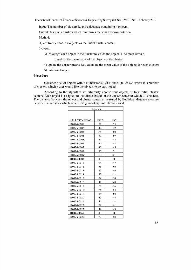
Input: The number of clusters k, and a database containing n objects.

Output: A set of k clusters which minimizes the squared-error criterion.

Method:

1) arbitrarily choose k objects as the initial cluster centers;

2) repeat

3) (re)assign each object to the cluster to which the object is the most similar,

based on the mean value of the objects in the cluster;

4) update the cluster means, i.e., calculate the mean value of the objects for each cluster;

5) until no change;

Procedure

Consider a set of objects with 2-Dimensions (PSCP and CO), let k=4 where k is numberof clusters which a user would like the objects to be partitioned.

According to the algorithm we arbitrarily choose four objects as four initial clustercenters. Each object is assigned to the cluster based on the cluster center to which it is nearest.The distance between the object and cluster center is measured by Euclidean distance measurebecause the variables which we are using are of type of interval-based.

Iteration0

HALL TICKET NO. PSCP CO

11087-i-0001 72 55

11087-i-0002 47 42

11087-i-0003 74 50

11087-i-0004 60 59

11087-i-0005 47 42

11087-i-0006 46 42

11087-i-0007 83 65

11087-i-0008 83 71

11087-i-0009 59 61

11087-i-0010 0 011087-i-0011 64 47

11087-i-0012 56 6611087-i-0013 67 49

11087-i-0014 57 5211087-i-0015 54 54

11087-i-0016 42 48

11087-i-0017 74 76

11087-i-0018 75 5411087-i-0019 84 6011087-i-0020 42 44

11087-i-0021 56 5811087-i-0022 59 61

11087-i-0023 49 4311087-i-0024 0 0

11087-i-0025 70 58




94

11087-i-0026 55 5011087-i-0027 53 70

11087-i-0028 77 7111087-i-0029 68 51

11087-i-0030 56 52

11087-i-0031 47 6211087-i-0032 72 64

11087-i-0033 67 43

11087-i-0034 0 0

11087-i-0035 80 66

11087-i-0036 0 011087-i-0037 42 42

11087-i-0038 67 54

11087-i-0039 70 49

11087-i-0040 73 60

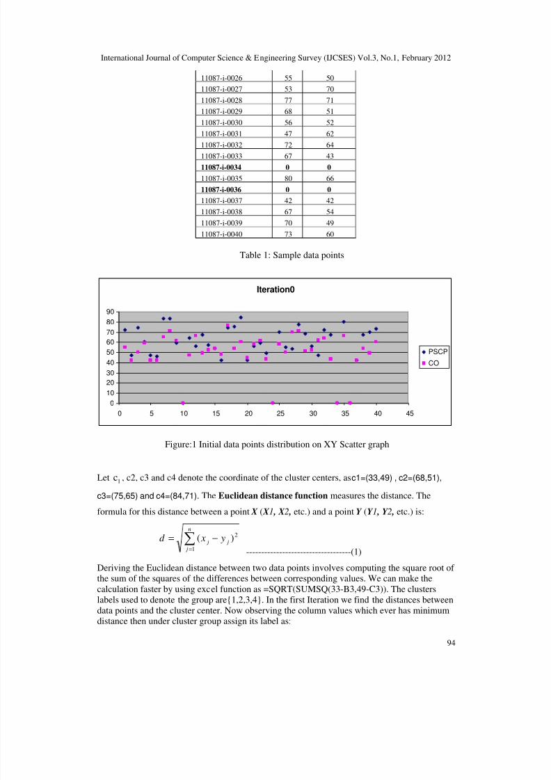
Table 1: Sample data points

Iteration0

0102030405060708090

0 5 10 15 20 25 30 35 40 45

PSCP

CO

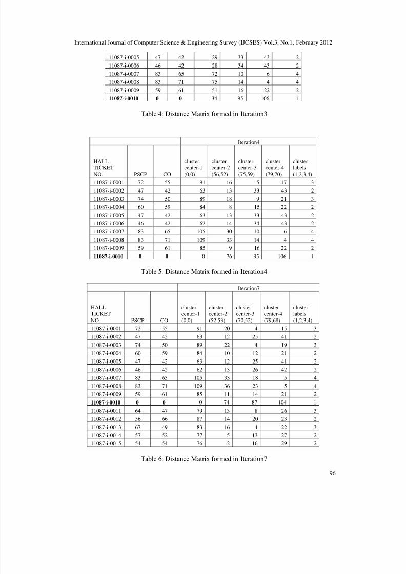
Figure:1 Initial data points distribution on XY Scatter graph

Let 1c , c2, c3 and c4 denote the coordinate of the cluster centers, as c1=(33,49) , c2=(68,51),

c3=(75,65) and c4=(84,71). The Euclidean distance function measures the distance. The

formula for this distance between a point X ( X 1 , X 2 , etc.) and a point Y (Y 1 , Y 2 , etc.) is:

∑=

−=n

j j j y xd

1

2)(-----------------------------------(1)

Deriving the Euclidean distance between two data points involves computing the square root of the sum of the squares of the differences between corresponding values. We can make thecalculation faster by using excel function as =SQRT(SUMSQ(33-B3,49-C3)). The clusterslabels used to denote the group are{1,2,3,4}. In the first Iteration we find the distances betweendata points and the cluster center. Now observing the column values which ever has minimumdistance then under cluster group assign its label as:




95

Iteration1

HALLTICKET NO. PSCP CO

clustercenter-1(33,49)




clusterlabels(1,2,3,4)

11087-i-0001 72 55 39 6 10 20 2

11087-i-0002 47 42 16 23 36 47 111087-i-0003 74 50 41 6 15 23 2

11087-i-0004 60 59 29 11 16 27 211087-i-0005 47 42 16 23 36 47 1

11087-i-0006 46 42 15 24 37 48 1

11087-i-0007 83 65 52 21 8 6 4

Table 2: Distance Matrix formed in Iteration1Next, the cluster centers are updated. That is, the mean value of each cluster is recalculatedbased on the current objects in the cluster. Using the new cluster centers, the objects areredistributed to the clusters based on which cluster center is the nearest. Hence after firstiteration the new cluster centers are cluster center-1 (30,30), cluster center-2 (63,54),cluster

center-3 (73,65) and cluster center-4 (80,71). Iteration2

HALL TICKETNO. PSCP CO






11087-i-0001 72 55 49 9 10 18 2

11087-i-0002 47 42 21 20 35 44 111087-i-0003 74 50 48 12 15 22 2

11087-i-0004 60 59 42 6 14 23 2

11087-i-0005 47 42 21 20 35 44 211087-i-0006 46 42 20 21 35 45 1

11087-i-0007 83 65 64 23 10 7 411087-i-0008 83 71 67 26 12 3 4

11087-i-0009 59 61 42 8 15 23 211087-i-0010 0 0 42 83 98 107 1

11087-i-0011 64 47 38 7 20 29 2

11087-i-0012 56 66 44 14 17 25 2

11087-i-0013 67 49 42 6 17 26 2

11087-i-0014 57 52 35 6 21 30 2

Table 3: Distance Matrix formed in Iteration2

This process of iteratively reassigning objects to clusters to improve the partitioning is referredto as iterative relocation. Eventually, no reassignment of the objects in the cluster occurs and sothe process terminates. The resulting clusters are returned by clustering process.

Iteration3






11087-i-0001 72 55 57 5 17 3

11087-i-0002 47 42 29 33 43 2

11087-i-0003 74 50 56 9 21 3

11087-i-0004 60 59 50 15 22 2




96

11087-i-0005 47 42 29 33 43 211087-i-0006 46 42 28 34 43 2

11087-i-0007 83 65 72 10 6 411087-i-0008 83 71 75 14 4 4

11087-i-0009 59 61 51 16 22 2

11087-i-0010 0 0 34 95 106 1


Iteration4

HALLTICKETNO. PSCP CO






11087-i-0001 72 55 91 16 5 17 3

11087-i-0002 47 42 63 13 33 43 2

11087-i-0003 74 50 89 18 9 21 311087-i-0004 60 59 84 8 15 22 211087-i-0005 47 42 63 13 33 43 2

11087-i-0006 46 42 62 14 34 43 2

11087-i-0007 83 65 105 30 10 6 4

11087-i-0008 83 71 109 33 14 4 4

11087-i-0009 59 61 85 9 16 22 2

11087-i-0010 0 0 0 76 95 106 1


Iteration7

HALLTICKETNO. PSCP CO






11087-i-0001 72 55 91 20 4 15 3

11087-i-0002 47 42 63 12 25 41 2

11087-i-0003 74 50 89 22 4 19 3

11087-i-0004 60 59 84 10 12 21 211087-i-0005 47 42 63 12 25 41 2

11087-i-0006 46 42 62 13 26 42 2

11087-i-0007 83 65 105 33 18 5 411087-i-0008 83 71 109 36 23 5 4

11087-i-0009 59 61 85 11 14 21 2

11087-i-0010 0 0 0 74 87 104 111087-i-0011 64 47 79 13 8 26 311087-i-0012 56 66 87 14 20 23 2

11087-i-0013 67 49 83 16 4 22 3

11087-i-0014 57 52 77 5 13 27 2

11087-i-0015 54 54 76 2 16 29 2





97

The k-means algorithm is applied on the 40 records with two attributes and to obtainfinal result, the algorithm under goes seven iteration and stops. After Iteration7 we see that thenew mean values obtained for four clusters are the same as that of previous step.

Figure 2: Final object distribution among four clusters

Instead of considering four clusters, if we consider six clusters (k=6) the algorithmiterates for two times and terminates as the mean values never change after it.

Iteration-1


clustercenter1(0,0)

clustercenter2(42,42)





clustergroup(1,2,3,4,5,6)

11087-i-0001 72 55 91 33 18 6 17 15 411087-i-0002 47 42 63 5 14 23 42 43 2

11087-i-0003 74 50 89 33 20 6 21 17 4

11087-i-0004 60 59 84 25 8 11 21 24 311087-i-0005 47 42 63 5 14 23 42 43 2

11087-i-0006 46 42 62 4 14 24 42 44 2

11087-i-0007 83 65 105 47 31 21 8 0 611087-i-0008 83 71 109 50 34 25 6 6 611087-i-0009 59 61 85 25 9 13 21 24 3

11087-i-0010 0 0 0 59 76 85 105 105 1

Table 7: Distance Matrix formed in Iteration1 for six clusters




98

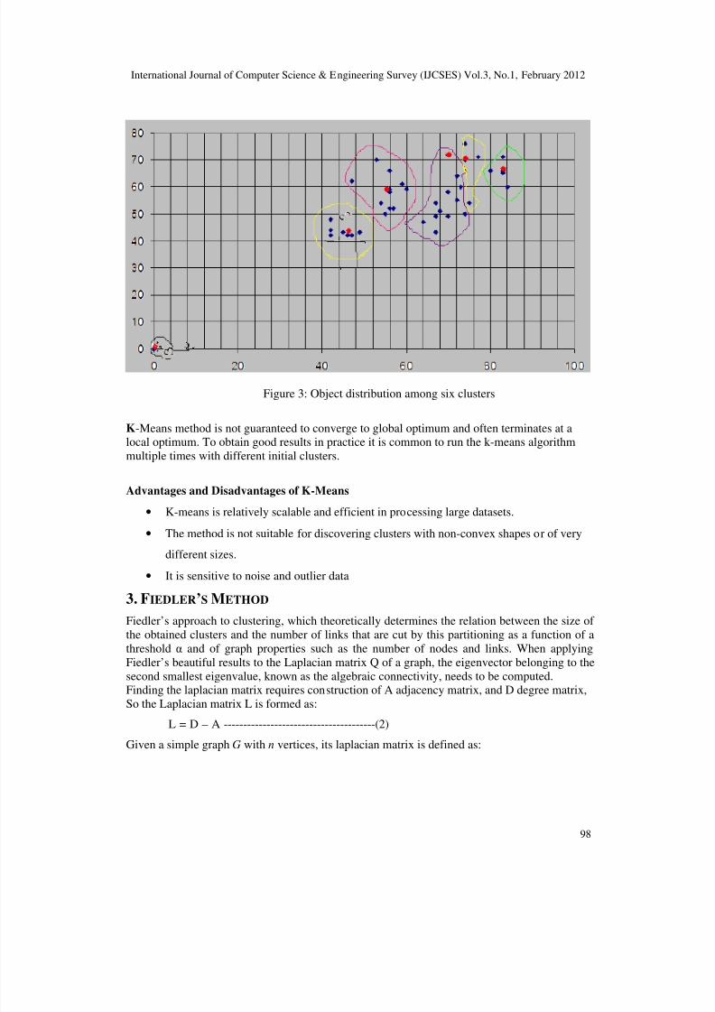
Figure 3: Object distribution among six clusters

K -Means method is not guaranteed to converge to global optimum and often terminates at alocal optimum. To obtain good results in practice it is common to run the k-means algorithmmultiple times with different initial clusters.

Advantages and Disadvantages of K-Means

• K-means is relatively scalable and efficient in processing large datasets.

• The method is not suitable for discovering clusters with non-convex shapes or of very

different sizes.

• It is sensitive to noise and outlier data

3. F IEDLER ’S M ETHOD Fiedler’s approach to clustering, which theoretically determines the relation between the size of the obtained clusters and the number of links that are cut by this partitioning as a function of athreshold α and of graph properties such as the number of nodes and links. When applyingFiedler’s beautiful results to the Laplacian matrix Q of a graph, the eigenvector belonging to thesecond smallest eigenvalue, known as the algebraic connectivity, needs to be computed.Finding the laplacian matrix requires construction of A adjacency matrix, and D degree matrix,

So the Laplacian matrix L is formed as:L = D – A ---------------------------------------(2)

Given a simple graph G with n vertices, its laplacian matrix is defined as:




99

Figure 4: Example graph

3.1 Adjacency Matrix

The adjacency matrix of a finite graph G of n vertices is the n × n matrix where the non-diagonal entry a ij is the number of edges from vertex i to vertex j, and the diagonal entry a ii, iseither once or twice the number of edges from vertex i to itself.

=

0000111100

0010000111

0100000001

0000000110

1000011000

1000101000

1000110000

1101000010

0101000100

0110000000

A

Figure 5: The adjacency matrix for the graph-1

3.2 Degree matrix

In the mathematical field of graph theory the degree matrix is a diagonal matrix which containsinformation about the degree of each vertex. That is the count of edges connecting a vertex v.If i ≠ j then replace the cell value with 0 other wise degree of the vertex v i

Figure 6: The degree matrix of graph-1

=

4000000000

0400000000

0020000000

0002000000

0000300000

0000030000

0000003000

0000000400

0000000030

0000000002

D




100

3.3 Laplacian matrix

Given a simple graph G with n vertices, its Laplacian matrix is defined as:L(i,j)=degree of vertex v i if i=j, if i ≠ j and v i is not adjacent to v j and in all other case fill it with 0.

Figure 7: the laplacian matrix for graph -1

3.4 Fiedler method

This method partitions the data set S into two sets S1 and S2 based on the eigen Vector Vcorresponding to the 2nd smallest eigen value of laplacian matrix. Consider the Equations

)3(n1........, j n

1k

−−−−−−−−−−−−−−== ∑=

k k ji xa y

Represent a linear transformation from the variables x 1,x2,…………..x n to the variables

y1,…………y n ; we can write this in matrix notation as Y=AX, where Y is a column vector and

A=(a ij) is matrix transformation. In many situations, we need to transform a vector into a scalar

multiple of itself.

i.e. AX= λ X--------------------------------------------------(4) where λ is a scalar.

Such problems are known as eign value problems. Let A be an n x n symmetric matrix and x isknown as eigen vector corresponding to the eigen values. To obtaine eigen vector we need to

solve (A- λ I)x=0. x=0 is a trivial solution of this linear system for any λ . For the system to have

a non-trivial solution, the matrix A- λ I must be singular. The scalar λ and the non-zero vector x

satisfying(4) exist if |A- λ I|=0.

pn(λ )=λ

λ

λ

−

−

nnn

n

aa

a

aa

....................a .

.

.

.....a..........-a

....................a

n21

2n2221

11211

=0.

By expansion of this determinant we get an nth degree polynomial in λ and p n(λ ) is known asthe characteristic polynomial of A and p n(λ )=0 as the characteristic equation of A. p n(λ )=0 has nroots, which may be real or complex. The roots are the eigen values of the matrix.As per Rayleigh Quotient Theorem Solution:

−−−−

−−−−

−−

−−

−−−

−−−

−−−

−−−−

−−−

−−

=

4000111100

0410000111

0120000001

0002000110

1000311000

1000131000

1000113000

1101000410

0101000130

0110000002

L




101

– λ 1=0, the smallest right-hand eigenvalue of the symmetric matrix , L

– λ 1 corresponds to the trivial eigenvector

v1= e = [1, 1, …, 1].

Based on a symmetric matrix, L, we search for the eigenvector, v 2, which is furthest away frome. Now v 2 gives relation information about the nodes. This relation is usually decided byseparating the values across zero.A theoretical justification is given by Miroslav Fiedler. Hence, v 2 is called the Fiedler vector.Hence v 2 is used to recursively partition the graph by separating the components into negativeand positive values.Entire Graph: sign(V)=[ +, +, +, -, -, -, +, +, +, -]

1 2 3 4 5 6 7 8 9 10

Iteration 1:Positives = [+, +, +, +, +, +]

1 2 3 7 8 9Negatives= [-, -, -, -]

4 5 6 10

Figure 12: Graph-1 after first iteration.

Sign(v2)=[+, -, -, -, +, +, ]1 2 3 7 8 9

Iteration 2:Positives =[+, +, + ]

1 8 9Negatives =[-, -, - ]

1 3 7

Figure 13: Graph after iteration -2




102

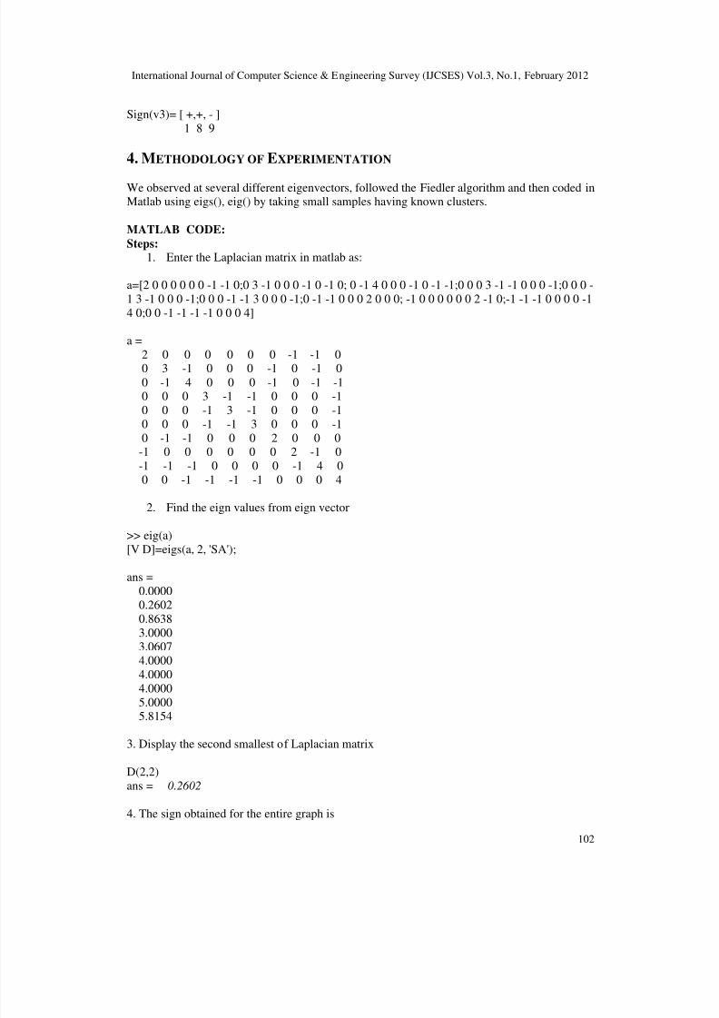
Sign(v3)= [ +,+, - ]1 8 9

4. M ETHODOLOGY OF E XPERIMENTATION

We observed at several different eigenvectors, followed the Fiedler algorithm and then coded inMatlab using eigs(), eig() by taking small samples having known clusters.

MATLAB CODE:Steps:

1. Enter the Laplacian matrix in matlab as:

a=[2 0 0 0 0 0 0 -1 -1 0;0 3 -1 0 0 0 -1 0 -1 0; 0 -1 4 0 0 0 -1 0 -1 -1;0 0 0 3 -1 -1 0 0 0 -1;0 0 0 -1 3 -1 0 0 0 -1;0 0 0 -1 -1 3 0 0 0 -1;0 -1 -1 0 0 0 2 0 0 0; -1 0 0 0 0 0 0 2 -1 0;-1 -1 -1 0 0 0 0 -14 0;0 0 -1 -1 -1 -1 0 0 0 4]

a =

2 0 0 0 0 0 0 -1 -1 00 3 -1 0 0 0 -1 0 -1 00 -1 4 0 0 0 -1 0 -1 -10 0 0 3 -1 -1 0 0 0 -10 0 0 -1 3 -1 0 0 0 -10 0 0 -1 -1 3 0 0 0 -10 -1 -1 0 0 0 2 0 0 0

-1 0 0 0 0 0 0 2 -1 0-1 -1 -1 0 0 0 0 -1 4 00 0 -1 -1 -1 -1 0 0 0 4

2. Find the eign values from eign vector

>> eig(a)[V D]=eigs(a, 2, 'SA');

ans =0.00000.26020.86383.00003.06074.00004.00004.00005.00005.8154

3. Display the second smallest of Laplacian matrix

D(2,2)ans = 0.2602

4. The sign obtained for the entire graph is




103

sign(V)=[ +, +, +, -, -, -, +, +, +, -]1 2 3 4 5 6 7 8 9 10

Iteration-2

a=[2 0 0 0 -1 -1;0 3 -1 -1 0 -1;0 -1 4 -1 0 -1;0 -1 -1 2 0 0;-1 0 0 0 2 -1;-1 -1 -1 0 -1 4][V D]=eigs(a,2,’SA’);D(2,2)ans = 0.8591

sign(V)= = [+, +, +, +, +, +]1 2 3 7 8 9

The final graph obtained for the graph-1

Figure 14: Plot-graph for the graph-1

4. CONCLUSIONThe advantage of the K-Means algorithm is its favorable execution time. Its drawback is that theuser has to know in advance how many clusters are searched for. It is observed that K-Meansalgorithm is efficient for smaller data sets only. Fielder’s method doesn’t require the preliminaryknowledge of the number of clusters, but most clustering methods require matrices to besymmetric. Symmetrizing techniques either distort original information or greatly increase thesize of the dataset moreover there are many applications where the data is not symmetric likeHyperlinks on the Web.




104

5. REFERENCES[1] Han, J. and Kamber, M. Data Mining: Concepts and Techniques, 2001 (Academic Press,

San Diego, California, USA).[2] Comparision between clustering algorithms- Osama Abu Abbas[3] Pham, D.T. and Afify, A.A. Clustering techniques and their applications in engineering.

Submitted to Proceedings of the Institution of Mechanical Engineers, Part C: Journal of Mechanical Engineering Science, 2006.

[4] Jain, A.K. and Dubes, R.C. Algorithms for Clustering Data, 1988 (Prentice Hall, EnglewoodCliffs, New Jersey, USA).

[5] Bottou, L. and Bengio, Y. Convergence properties of the k-means algorithm.[6] B. Mohar, The Laplacian Spectra of Graphs. Graph Theory, Combinatorics, and

Applications, Wiley, pp. 871, 1991.[7] D. Cvetkovi´c, P. Rowlinson, S. Simi´c. An introduction to the Theory of Graph

Spectra.Addison-Wesley, Cambridge University Press, 2010.

[8] P. Van Mieghem. Performance Analysis of Communications Networks and Systems.Addison-Wesley, Cambridge University Press, 2006.

Author

T. Soni Madhulatha obtained MCA from Kakatiya University in 2003 andM. Tech (CSE) from JNTUH in 2010.She has 8 years of teachingexperience and she is presently working as Associate professor inDepartment of Informatics in Alluri Institute of Management Sciences,Hunter Road Warangal. She published papers in various National andInternational Journals and Conferences. She is a Life Member of ISTE ,IAENG and APSMS.

Graph Partitioning Advance Clustering Technique

Documents

Transcript of Graph Partitioning Advance Clustering Technique