Graph kernel based aromaticity predictionAbstract Aromaticity is an important property of molecules,...

University of Freiburg

Bachelor Thesis

Graph kernel based aromaticityprediction

thesis submitted in fulfilment of the requirements

for the degree of Bachelor of Science

in the

Chair for Bioinformatics

Department of Computer Science

Done by:

Daniela Putz

Supervisors:

Dr. Martin Mann and Dr. Fabrizio Costa

Reviewers:

Prof. Dr. Rolf Backofen

Jun.-Prof. Dr. Stefan Gunther

August 2013

Abstract

Aromaticity is an important property of molecules, but has no real definition. Dif-

ferent tools exist, but they can not accurately predict aromaticity. Because of this a

graph kernel machine learning tool by F. Costa was modified to be trained to recognize

aromaticity.

In this thesis first a molecule database was converted to SMILES format without aro-

maticity information. On these SMILES a selection of popular aromaticity perception

tools was used. Then the machine learning tool was trained and tested on their output

and also applied to the original SMILES. The goal was to evaluate the different tools

and to test the performance of a machine learning tool.

ii

Zusammenfassung

Aromen sind ein wichtiger Bestandteil moderner Chemie, und dennoch gibt es keine

Definition, die sie eindeutig definiert. Es gibt eine Auswahl an regelbasierten Methoden,

doch diese liefern unterschiedliche Ergebnisse. Deshalb wurde ein Graph Kernel von

F.Costa modifiziert, um von Molekulgraphen, die aromatisch sind, zu lernen und somit

bessere Ergebnisse zu liefern, als es die heutigen Me-thoden tun.

In dieser Arbeit wurde zunachst eine bekannte Molekuldatenbank in das Format SMILES

umgewandelt, um dann eine Auswahl an Methoden darauf anzuwenden, die Aromaten

erkennen. Auf deren Ausgaben wurde dann das Machine Learning Tool trainiert, und

schließlich auch auf den ursprunglichen SMILES angewendet, um die Aromaten zu erken-

nen. Das Ziel war es, die einzelnen Methoden zu evaluieren um herauszufinden, wie gut

ein Machine Learning Tool dafur geeignet ist, Aromaten zu erkennen.

iii

Contents

Abstract ii

Zusammenfassung iii

List of Figures vi

List of Tables vii

Abbreviations viii

1 Introduction 1

1.1 Motivation . . . . . . . . . . . . . . . . . . . . . . . . . . . . . . . . . . . 1

1.1.1 Aromaticity . . . . . . . . . . . . . . . . . . . . . . . . . . . . . . . 2

1.1.2 Problems . . . . . . . . . . . . . . . . . . . . . . . . . . . . . . . . 4

1.2 New solution: The graph kernel . . . . . . . . . . . . . . . . . . . . . . . . 5

1.3 Outline . . . . . . . . . . . . . . . . . . . . . . . . . . . . . . . . . . . . . 6

2 Data and methods 7

2.1 Data . . . . . . . . . . . . . . . . . . . . . . . . . . . . . . . . . . . . . . . 7

2.1.1 The database used . . . . . . . . . . . . . . . . . . . . . . . . . . . 7

2.1.2 Preparation of the data . . . . . . . . . . . . . . . . . . . . . . . . 8

2.2 Aromaticity perception tools . . . . . . . . . . . . . . . . . . . . . . . . . 10

2.2.1 Marvin . . . . . . . . . . . . . . . . . . . . . . . . . . . . . . . . . 10

2.2.2 OpenBabel . . . . . . . . . . . . . . . . . . . . . . . . . . . . . . . 11

2.2.3 Daylight and CDK . . . . . . . . . . . . . . . . . . . . . . . . . . . 12

2.3 Applying the tools . . . . . . . . . . . . . . . . . . . . . . . . . . . . . . . 12

2.4 Preparing the data for evaluation . . . . . . . . . . . . . . . . . . . . . . . 13

3 The machine learning tool 16

3.1 The graph kernel . . . . . . . . . . . . . . . . . . . . . . . . . . . . . . . . 16

3.2 The SVM . . . . . . . . . . . . . . . . . . . . . . . . . . . . . . . . . . . . 17

3.3 Model generation and evaluation . . . . . . . . . . . . . . . . . . . . . . . 18

3.4 Applying the models . . . . . . . . . . . . . . . . . . . . . . . . . . . . . . 19

4 Results 20

4.1 Evaluation . . . . . . . . . . . . . . . . . . . . . . . . . . . . . . . . . . . . 20

4.2 Results for the whole data sets . . . . . . . . . . . . . . . . . . . . . . . . 21

iv

Contents v

4.3 Results for the heterogeneous data sets . . . . . . . . . . . . . . . . . . . . 26

5 Discussion and conclusion 30

Bibliography 32

Selbststandigkeitserklarung 34

List of Figures

1.1 An example molecule (beta-thujaplicin) in graph representation. Source:Daylight Depict (aromaticity removed) [1] . . . . . . . . . . . . . . . . . . 1

1.2 A graphical representation of the delocalized electrons of benzene. Theorbitals (left) overlap and the electrons are free to cycle the ring (right).Source: Wikipedia [2] . . . . . . . . . . . . . . . . . . . . . . . . . . . . . 2

1.3 The two Kekule structures (top) and a representation of the delocalizedelectrons (bottom) for Benzene. Source: Wikipedia [2] . . . . . . . . . . . 3

2.1 The example molecule (beta-thujaplicin) from figure 1.1 (Chapter 1), onlythe parts that are converted: the molfile. . . . . . . . . . . . . . . . . . . . 8

2.2 The same molecule as in figure 1.1 and 2.1, this time represented in GML. 9

2.3 Graphical representation of pyrrole, as an example for the pattern of 5-membered rings ambiguous checks. Source: Wikipedia [3] . . . . . . . . . 11

2.4 (a) The five-membered rings loose consideres to be aromatic, where: A =any atom except hydrogen, Q = any atom except H or C(b) The six-membered rings loose consideres to be aromatic(c) The perimeter bonds in azulenes loose consideres to be aromaticSource: chemaxon.com [4] . . . . . . . . . . . . . . . . . . . . . . . . . . . 12

3.1 (a): Relabeling (b): to encode uncertainty about aromaticity of ring sys-tem and (c): single ring query via vertex/edge relabeling with the graphkernel. Source: Data-driven aromatic ring prediction with graph kernelsM.Mann et al. [5] . . . . . . . . . . . . . . . . . . . . . . . . . . . . . . . . 16

3.2 Single features of the graph kernel for distance D=5 and radius R=1, 2and 3 (left, center, right). Source: NSPDK F.Costa et al. [6] . . . . . . . 17

vi

List of Tables

2.1 Number of errors and SMILES with components in the output of eacharomaticity tool and number of SMILES in this output . . . . . . . . . . . 12

2.2 SMILES output for the example molecule (beta-thujaplicin) from figure1.1 for different aromaticity tools. . . . . . . . . . . . . . . . . . . . . . . . 13

2.3 Crashes of molMatch . . . . . . . . . . . . . . . . . . . . . . . . . . . . . 14

2.4 Number of output structural keys of annotateRings.pl (basically minusthe 48 molRing crashes) . . . . . . . . . . . . . . . . . . . . . . . . . . . . 15

2.5 Number of structural keys in each of the data sets and what percentagethat is of the original set. In this case it has size 16922 (see table 2.4)since only molecules in the smallest set can be part of the new sets (sincethe lines where one of the tools has an error tag are ignored) . . . . . . . 15

3.1 Merged statistic of the tests of the two SVM models with FeatureBitSize=15 19

3.2 Merged statistics of the tests of the two SVM models with FeatureBit-Size=22 default . . . . . . . . . . . . . . . . . . . . . . . . . . . . . . . . . 19

4.1 Heatmaps of the percentage of equal structural keys, pairwise for each tool. 23

4.2 Heatmaps of the average Tanimoto coefficient of the structural keys, pair-wise for each tool. . . . . . . . . . . . . . . . . . . . . . . . . . . . . . . . 24

4.3 Evaluation of the percentage of equal structural keys in the data sets(each subtable), pairwise for each of the tools . . . . . . . . . . . . . . . . 25

4.4 Percentages and number of rows where at least one tool gave a differentresult in the evaluation. First without considering the SVM and percent-age of old, then with all tools considered. . . . . . . . . . . . . . . . . . . 26

4.5 Heatmaps of the percentage of equal structural keys, pairwise for eachtool. Heterogeneous data sets. . . . . . . . . . . . . . . . . . . . . . . . . . 27

4.6 Heatmaps of the average Tanimoto coefficient of the structural keys, pair-wise for each tool. Heterogeneous data sets. . . . . . . . . . . . . . . . . . 28

4.7 Evaluation of the percentage of equal structural keys in the heterogeneousdata sets (each subtable), pairwise for each of the tools . . . . . . . . . . . 29

5.1 Whole data set, (a) Average of percentage result of each tool compared toall other tools (except the SVM) and (b) the results of the SVM comparedto this tool . . . . . . . . . . . . . . . . . . . . . . . . . . . . . . . . . . . 31

5.2 Whole heterogeneous data set, (a) Average of percentage result of eachtool compared to all other tools (except the SVM) and (b) the results ofthe SVM compared to this tool . . . . . . . . . . . . . . . . . . . . . . . . 31

vii

Abbreviations

SDF Structure-Data File

GML Graph Modelling Language

SMILES Simplified Molecular-Input Line-Entry System

SVM Support Vector Machine

NSPDK Neighborhood Subgraph Pairwise Distance Kernel

CDK Chemistry Development Kit

GGL Graph Grammar Library

viii

Chapter 1

Introduction

1.1 Motivation

A molecule is the smallest particle of a substance, e.g. H2O is the molecule that makes up

water. Molecules consists of two or more atoms being held together by shared electron

pairs, i.e. chemical bonds. This can be represented as a graph, where each atom is

encoded as a vertex and single, double or triple bonds (bonds where two, four or six

electrons are shared, respectively) are represented by an according number of edges [7].

Figure 1.1 shows an example of a molecule in graph representation.

Figure 1.1: An example molecule (beta-thujaplicin) in graph representation. Source:Daylight Depict (aromaticity removed) [1]

The chemical properties of each molecule are determined by the type of the atoms it

contains, combined with its structure. These properties have a large influence on the

reactivity of the substance. One of them, aromaticity, is the topic of this thesis.

1

Chapter 1. Introduction 2

1.1.1 Aromaticity

Aromaticity is a fundamental concept of chemistry, yet not directly measurable or even

completely understood [8].

It was introduced to explain the properties of benzene, which still is considered to be the

most typical aromatic molecule (figures 1.2 and 1.3 both show benzene). The benzene

ring is a conjugated ring with two Kekule structures (see definition 1.5 and the two

structures in figure 1.3). It is especially stable, more so than the conjugation alone can

explain (see definition 1.4). Other molecules also exhibiting this heightened stability

were found, and these could be explained with aromaticity [9]. However, there are more

criteria for aromaticity that will be introduced further down.

Definition 1.1. An orbital is a region around the atom where the electron is likely to

be [9].

Definition 1.2. A π-bond describes the overlap of two adjacent orbitals between two

atoms.

A π-electron is an electron participating in a π-bond [9].

Figure 1.2: A graphical representation of the delocalized electrons of benzene. Theorbitals (left) overlap and the electrons are free to cycle the ring (right). Source:

Wikipedia [2]

Definition 1.3. An electron is localized if it is located inside the electron cloud of

an atom or bond and delocalized if it is not associated with an atom or one bond,

but rather in an orbital extending over several adjacent atoms [9]. See figure 1.2 for a

graphical representation of the delocalized electrons.


Definition 1.4. A ring of atoms is considered to be conjugated if it consists of al-

ternating single and double bonds and π-electrons are delocalized across all adjacent

p-orbitals. These π-electrons are free to cycle the ring, belonging to it and not a single

atom [9].

Definition 1.5. Some molecules have rings where the double and single bond assignment

is ambivalent, leading to more than one graph representation being possible. These are

called Kekule structures. This is caused by the delocalized electrons participating

in different bonds at different times, causing the bonds to constantly switch between

single and double [9]. Figure 1.3 shows the two graphs and the representation of the

delocalized electrons of benzene.

Figure 1.3: The two Kekule structures (top) and a representation of the delocalizedelectrons (bottom) for Benzene. Source: Wikipedia [2]

Definition 1.6. Bond length equalization occurs when the delocalized electrons are

shared by all atoms, and strengthen the bonds. Since there are not enough electrons

to form double bonds between all atoms, the bonds turn intermediate in strength and

length between single and double bonds [9].

Definition 1.7. The Huckel rule : 4n + 2 = number of π-electrons, where n is zero

or any positive integer, is commonly used to determine if a ring or molecule has aro-

maticity. During 1931-1938 Erich Huckel developed the basic patterns of orbital theory.


He concluded, that the binding energy would vary with the number of π-electrons, and

that systems with 4n + 2 of them would have a particularly high energy and thus be

especially stable and probably aromatic [10].

Aromaticity means different things to different fields of science, depending on how it

affects their respective work. So there is basically a structural, a magnetic and an

energetic ”definition”.

structural: the more symmetric a molecule is, the more aromatic it is. The symmetry

is caused by the bond length equalization of the conjugated ring [8].

magnetic: an external magnetic field induces a relatively high ring current in the π-

electrons. This current creates a magnetic field that is opposed at the center of the ring

and has the same direction at the outside of the ring as the external field [8].

energetic: the molecule shows heightened kinetic and thermodynamic stability. This is

determined in comparison with a reference system, e.g. by the heat of formation, which

is the energy released when one mol is created from the elements (negative) or which is

necessary for the formation of the molecule (positive). However, this is not a well suited

reference system for determining aromaticity, so usually other systems are used [8].

1.1.2 Problems

The criteria from above are rather problematic, as shown below:

structural: There exist counterexamples, which are not aromatic, that are actually

more symmetrical than aromatic molecules, so this criterion is a very weak one [8].

magnetic: Again, there exist systems exhibiting this property that are not aromatic,

but in general it works better than the structural criteria [8].

energetic: Stability is a relative term, and highly dependent on reference systems. So

different reference systems can lead to different aromaticity assignments. But stability

is undeniably a defining factor of aromaticity [8].

So they are only empiric methods, not real definitions. Even so, they usually work well

enough on the prototypes, and might even correlate well between each other for those

”usual” systems, for which aromaticity has long been assigned.


Still, aromaticity has a large effect on the physical and chemical properties of a molecule

and it is therefore important to accurately predict it. It is also difficult to canonicalize

databases if the aromaticity is unknown or, even worse, different tools lead to different

aromaticity assignments. The various Kekule structures of aromatic molecules also pose

a problem, since most methods for computer representation and storage (e.g. SMILES)

cannot connect them to the aromatic molecule. Here, an aromaticity prediction and a

special handling is essential to overcome this problem [11]. Furthermore many algorithms

use aromaticity to generate structural fingerprints or to assign hydrogens [5].

Daylight even warns that their aromaticity assignment has nothing to do with any of

these ”definitions”:

”It is important to remember that the purpose of the SMILES aromaticity

detection algorithm is for the purposes of chemical information represen-

tation only! To this end, rigorous rules are provided for determining the

”aromaticity” of charged, heterocyclic, and electron-deficient ring systems.

The ”aromaticity” designation as used here is not intended to imply any-

thing about the reactivity, magnetic resonance spectra, heat of formation, or

odor of substances.”

Source: Daylight website [12]

1.2 New solution: The graph kernel

The Huckel rule (definition 1.7) is often used to determine aromaticity, even though it

fails for many molecules. Most of the tools used nowadays are based on it, and handle

exceptions explicitly. But none of them cover all the methods for recognizing aromaticity.

Because of this a data-driven approach was proposed by M.Mann and F.Costa [5]. For

this purpose the machine learning tool NSPDK by F.Costa et al. [6] was used, since

the molecules can be represented as graphs. Given a large enough set of reliable data

with correct aromaticity information it will be able to accurately predict aromaticity.

The problem is that there exists no such data set, yet, since there is no accurate way of

predicting aromaticity and it would have to be thoroughly checked.


So, until such a database is created, the tool can also be trained on the results of other

tools. Because none of the methods for aromaticity detection is accurate, an SVM

trained on their combined output probably achieves better result than each of them,

since hopefully the problems of each tool will be compensated by the predictions of the

other tools.

This is what will be done in this thesis for a selection of tools, so the performance of the

SVM can be evaluated compared to each of the tools.

1.3 Outline

In the next chapter first the data used is introduced and the way it was prepared, so

the aromaticity tools could be applied and the output could be evaluated. The tools are

also explained. In chapter 3 the SVM is explained and it is shown how the SVM was

trained, tested and applied. Then in chapter 4 the results of the pairwise comparison

of all tools and the SVM are displayed and described. These results are discussed in

chapter 5.

Chapter 2

Data and methods

2.1 Data

2.1.1 The database used

ChEBI is a database of small molecules of biological interest, the version used in this

thesis, ChEBI complete 3star in SDF format contains 26347 molecules. The 3star

indicates that entries have been manually annotated by the ChEBI team. All of them

are either the result of a natural chemical process or synthetic products that influence

processes in living organisms. Molecules coded by the genome however are not part of

it, thus excluding nucleic acids and proteins [13].

Because of the limited size of the graphs the SVM will have to work with and the large

number of aromatic molecules in it, this database is especially suited to evaluate the

different aromaticity perception tools and the SVM.

The version in SDF format was used in this thesis [14]. SDF is a format that wraps

the molfile shown in figure 2.1 (third line from above to 6th from below). Each entry

contains a molfile and further information about the molecule it represents.

The molfile format looks like this: A header line (line 3 in the example in figure 2.1),

containing the atom and bond count at the first and second position. Then for each

atom a line, containing further information and the atom type at position 4 (lines 4 to

12 in the example), and for each bond a line, containing the indices of the end atoms in

position 1 and 2 and a number encoding the bond type at position 3 (lines 13-24).

7

Chapter 2. Data and methods 8

That is all that is needed to create a molecule graph.

Figure 2.1: The example molecule (beta-thujaplicin) from figure 1.1 (Chapter 1), onlythe parts that are converted: the molfile.

2.1.2 Preparation of the data

Since all of the aromaticity perception tools work with SMILES as input, the database

needed to be converted into that format. SMILES are a compact string representation

of molecules, coding aromaticity with lowercase symbols [15].

The initial SMILES for prediction were supposed to be without any aromaticity infor-

mation, thus a converter from SDF to GML was written, such that the program molTool

of the GGL toolkit [16], that converts a molecule in GML to SMILES and vice versa,

could be used to convert the GML to SMILES.

It was also needed, because this way the node index of the graphs would be the same

as in the SDF, so the rings could be identified. The aromaticity could then later be

mapped to these GML graphs (see Chapter 4 to find the aromatic rings).


The converter only uses the information in the molfile, transforming atoms into vertices

and bonds into edges (example in figure 2.2). Individually connected components were

split up into separate molecules. Each graph in GML was written into a single line. The

ChEBI ID was kept in a separate file, with corresponding line numbers, so the GML

graphs and later the SMILES can easily be matched to their molecules and ChEBI

entries.

Some of the ChEBI entries contained non-valid atom names and were thus ignored.

Others contained hydrogen only. Overall 640 molecules were filtered out this way. This

left 25707 molecules to be converted.

Figure 2.2: The same molecule as in figure 1.1 and 2.1, this time represented in GML.

Using molTool, each of the lines of the GML file was converted into a SMILES without

aromaticity. At this point the SMILES were filtered for rings, since aromaticity only

occurs in rings and the SMILES format makes them easy to find. A simple perl script

took care of that. This left 17014 molecules to be considered in this study.


2.2 Aromaticity perception tools

Popular tools for aromaticity perception are Daylight, CDK, OpenBabel and Marvin. In

this thesis Daylight and CDK were not used (see 2.2.3 ”Daylight and CDK”), thus leaving

only the babel method and the four methods of Marvin: general, basic, ambiguous and

loose. However ambiguous was also not used further (see definition 2.3).

2.2.1 Marvin

Definition 2.1. General [4]: Sum the number of π-electrons of atoms in rings with

alternating single and double bonds. Check if the Huckel rule (see definition 1.7) is valid.

If it is, the ring is declared aromatic. This is the same method as used by Daylight.

Exceptions:

� Oxygen and sulfur can share a pair of π-electrons.

� Nitrogen can also share a pair of π-electrons, if it has three ions or molecules bound

to it, otherwise the nitrogen shares only one electron.

� An exocyclic double bond to an electronegative atom takes out one shared π-

electron from the cycle, as in 2-pyridone or coumarin.

� It also checks ring systems, but the atoms at the generated ring system may not

form a continuous ring.

Definition 2.2. Basic [4]: This method is similar to the General method, but it has

different exceptions:

� A ring can be aromatic without having sequential double and single bonds. In this

case the atom between single bonds has an orbit which takes part in the aromatic

system.

� Rings with less than 5 members are not considered aromatic.

Difference General and Basic: The general method tries to include Kekule structures,

while the basic method does not. In the basic method the external double bond breaks

the formation of an aromatic ring [4].


Definition 2.3. Ambiguous [4]: checks 5-membered rings with bond pattern similar

to pyrrole (see figure 2.3). In that particular ring, the bonds are replaced by ”single

or aromatic” and ”double or aromatic” bonds. In case of 5-membered ring fusion with

aromatic rings, the aromatic ring is aromaticized first. Ambiguous fails for over 4000

of the SMILES (see table 2.1), and thus was not used further in this thesis because it

constrains the data too much.

Figure 2.3: Graphical representation of pyrrole, as an example for the pattern of5-membered rings ambiguous checks. Source: Wikipedia [3]

Definition 2.4. Loose [4]: As the name implies this method only has a very loose

definition of aromaticity. It interprets the following ring systems as aromatic:

� Five-membered rings like the structures shown in figures 2.4 (a) (Where: A = any

atom except hydrogen, Q = any atom except H or C)

� Six-membered rings that can be drawn as alternating single and double bonds, like

the structures in figure 2.4 (b)

� Perimeter bonds in azulenes, like the structure shown in figure 2.4 (c)

2.2.2 OpenBabel

The OpenBabel method babel is similar to the Daylight/General method, but with

added support for aromatic phosphorous and selenium.

Potential aromatic atoms and bonds are flagged according to the Huckel rule. Aromatic-

ity is only assigned if a well-defined valence bond Kekule pattern can be determined.

To do this, atoms are added to a ring system and the Huckel rule is checked for every

one, gradually increasing the size to find the largest possible connected aromatic ring

system.


Figure 2.4: (a) The five-membered rings loose consideres to be aromatic, where: A= any atom except hydrogen, Q = any atom except H or C(b) The six-membered rings loose consideres to be aromatic

(c) The perimeter bonds in azulenes loose consideres to be aromaticSource: chemaxon.com [4]

Once this ring system is determined, an exhaustive search is performed to assign single

and double bonds to satisfy all valences in a Kekule form [17].

2.2.3 Daylight and CDK

Daylight: Daylight has modified and extended the SMILES language, and their method

of aromaticity perception is implemented into the SMILES algorithm. It is also imple-

mented in Marvin, as the general method (see definition 2.1).

CDK: has been left out because it is almost the same as the basic method (see definition

2.2).

2.3 Applying the tools

tool failures component SMILES number output SMILES

babel 0 0 17014general 0 38 16976basic 1 38 16975

ambiguous 4146 37 12831loose 2 38 16974

Table 2.1: Number of errors and SMILES with components in the output of eacharomaticity tool and number of SMILES in this output


tool SMILES

OpenBabel CC(C)c1cccc(=O)c(O)c1

basic CC(C)C1=CC=CC(=O)C(O)=C1

general CC(C)c1cccc(=O)c(O)c1

loose CC(C)C1=CC=CC(=O)C(O)=C1

Table 2.2: SMILES output for the example molecule (beta-thujaplicin) from figure1.1 for different aromaticity tools.

Each of the aromaticity perception tools was used with ring SMILES as input, producing

5 files with SMILES containing aromaticity information. The Marvin methods crashed

on some of the SMILES, in place of which blank lines were left. See table 2.1, column

”failures” for an according listing. This happened especially often with the ambiguous

method, where almost a quarter of the input (24,37%) was not processed. Due to this

reason, the method was left out from the study.

Apparently due to a bug in Marvin, some of the single molecules resulted in multi-

molecule SMILES (see column ”component SMILES” in table 2.1). They were marked

with an error tag in place of the SMILES and ignored later on.

2.4 Preparing the data for evaluation

The tool molMatch from the GGL toolkit [16] maps a SMILES with aromaticity infor-

mation onto the GML graph of the same molecule, producing GML with aromaticity

information with the same node indices as the original GML.

All tools reported their aromaticity assignment in SMILES format. In order to make the

assignments comparable, the SMILES had to be converted into a unified graph format,

with identical node indexing.

First, to this end, each SMILES without aromaticity information was converted into a

GML graph, utilizing the −noProtonRemoval option to generate a full graph represen-

tation [16]. This new GML encoding was then, together with the aromaticized SMILES,

used as input for molMatch, merging each SMILES with its corresponding GML graph

and creating GML with aromaticity information and identical node indexing. The times

molMatch crashed on the SMILES of each tool can be looked up in table 2.3.


tool crashes number of output molecules

babel: 6 17008general: 2 16974basic: 5 16970loose: 4 16970

Table 2.3: Crashes of molMatch

The GML output of molTool was further used as input for molRings, extracting the

ring information. molRings is another tool part of the GGL toolkit [16], it takes a

molecule in GML format and finds all the rings in the molecules, producing a code for

each molecule like this:

atom1 − atom2 − ...− atomn : atomn+1 − ....− atomm : ... :

where multiple rings are separated by ”:” and 1, 2, ..., n,m are the atom IDs, or node

indices of the GML.

molRings crashed on 48 of the GML graphs, thus leaving 16966 molecules for further

use. The ring code for the example molecule (beta-thujaplicin see figure 1.1) is given in

the following:

9− 7− 6− 5− 4− 3− 11− 9 :

Definition 2.5. Structural key [12]: A bitstring where each bit represents the presence

or absence of a structural quality in the molecule. In this thesis this structural quality

is aromaticity. An example structural key would be 101, which represents a molecule

containing three rings, two of which are aromatic.

On this file and each of the aromatic GML files, annotateRings.pl by Martin Mann was

called, creating structural keys (see definition 2.5) encoding the aromaticity for each

molecule. In table 2.4 the number of output structural keys of each tool that were

further used for the evaluation are listed.

The structural keys were split into data sets according to ring count, leaving out the

ones with error tags in any of the tools. Overall there were 100 lines where this was the

case. This way eight data sets were created, with structural keys encoding 1, 2, 3, 4, 5,

6-10, more than 11 rings and one with all numbers of rings. Each data set contained for


tool number of structural keys

babel: 16966general: 16926basic: 16922loose: 16922

Table 2.4: Number of output structural keys of annotateRings.pl (basically minusthe 48 molRing crashes)

data set number of structural keys percentage of smallest original data set

ring1 4729 27.95%ring2 3383 19.99%ring3 3551 20.98%ring4 2465 14.57%ring5 1116 6.59%

ring6-10 1277 7.55%ring11+ 393 2.32%all rings 16914 99.95%

Table 2.5: Number of structural keys in each of the data sets and what percentagethat is of the original set. In this case it has size 16922 (see table 2.4) since onlymolecules in the smallest set can be part of the new sets (since the lines where one of

the tools has an error tag are ignored)

each molecule the structural key for each tool for the final evaluation. The size of the

data sets, and the percentage this is of the smallest original data set, is listed in table

2.5.

Chapter 3

The machine learning tool

3.1 The graph kernel

A graph kernel is basically a function measuring the similarity of graphs. In this thesis

a modified version of the NSPDK by F.Costa was used.

Figure 3.1: (a): Relabeling (b): to encode uncertainty about aromaticity of ringsystem and (c): single ring query via vertex/edge relabeling with the graph kernel.

Source: Data-driven aromatic ring prediction with graph kernels M.Mann et al. [5]

Each molecule is represented as a graph in which bonds and nodes participating in a

ring (since aromaticity only occurs in rings) are labeled with a special notation, coding

uncertainty about their aromaticity, since the actual label is unknown. For each ring

in each molecule graph the graph is saved as an instance where the ring in question is

marked (green in figure 3.1). This is the ring for which aromaticity is predicted.

16

Chapter 3. The machine learning tool 17

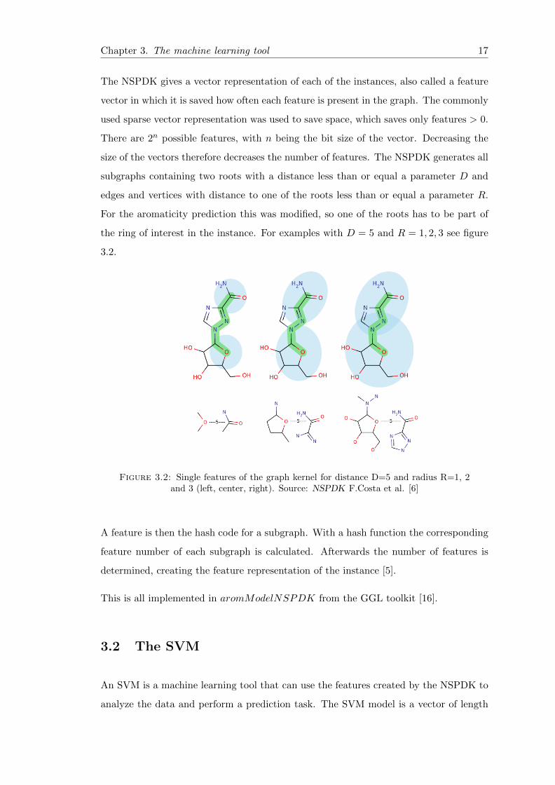
The NSPDK gives a vector representation of each of the instances, also called a feature

vector in which it is saved how often each feature is present in the graph. The commonly

used sparse vector representation was used to save space, which saves only features > 0.

There are 2n possible features, with n being the bit size of the vector. Decreasing the

size of the vectors therefore decreases the number of features. The NSPDK generates all

subgraphs containing two roots with a distance less than or equal a parameter D and

edges and vertices with distance to one of the roots less than or equal a parameter R.

For the aromaticity prediction this was modified, so one of the roots has to be part of

the ring of interest in the instance. For examples with D = 5 and R = 1, 2, 3 see figure

3.2.

Figure 3.2: Single features of the graph kernel for distance D=5 and radius R=1, 2and 3 (left, center, right). Source: NSPDK F.Costa et al. [6]

A feature is then the hash code for a subgraph. With a hash function the corresponding

feature number of each subgraph is calculated. Afterwards the number of features is

determined, creating the feature representation of the instance [5].

This is all implemented in aromModelNSPDK from the GGL toolkit [16].

3.2 The SVM

An SVM is a machine learning tool that can use the features created by the NSPDK to

analyze the data and perform a prediction task. The SVM model is a vector of length


2n, where n is the bit length of the feature vector, that assigns a weight to each feature.

The score of a model against a feature vector is calculated by simple scalar multiplying

the two vectors. With the SVM used in the thesis, if the score is greater than 0 the

model is aromatic, else it is not.

This model has to be trained to acquire information about the aromaticity. For this

a large enough amount of feature vectors and target scores not equal zero are needed.

Usually the model is trained with only score -1 and 1. On this training data a training

tool, in this case the Stochastic Gradient Descent, is used to find the model that gives

the best results, closest to the scores of the training data [5].

3.3 Model generation and evaluation

In order to acquire a meaningful statistic the SVM has to be cross-validated, i.e. models

trained on one part of the data have to be tested on another so the performance would

be independent of the training set. The training data is randomly partitioned into k sets

of equal size and a model is trained on all combinations of k− 1 sets and then tested on

the remaining set.

Because the training data set is so huge, only k = 2 was needed to give meaningful

results.

Thus the aromatic SMILES of all tools were randomly split up into two sets, using

modelAssign by Martin Mann. It takes a number of lines and produces a model id map

randomly filled with half the input number of 1s and half the input number of 2s.

The script was called on the number of lines in each SMILES file, which was 17014. With

the resulting model ID map the SMILES for each tool were split into the corresponding

model files.

On each of these two files a model was trained using aromModelNSPDK.

The option −nspdkFeatureBitSize was set to 15 and 22 to see what influence it has

when there are less feature vectors. This made quite the difference in the size of the

output model files, while the performance stayed almost the same (see tables 3.1, which

shows the performance with featurebitsize = 15 and 3.2, with featurebitsize = 22). The


file for model 1 was 5.645KiB with the default setting and 652KiB with it set to 15.

With model 2 it was 5.393KiB and 653KiB.

Therefore, in the remaining thesis only the smaller models with 15 bits were used.

The resulting models were each tested on the half not used for their training, merging

the statistics output of both models.

overall rings correct 215676 / 222765 96.8177 %aromatic rings correct 77948 / 83316 93.557 %non-aromatic r correct 137728 / 139449 98.7659 %whole molecule correct 62411 / 68053 91.7094 %

Table 3.1: Merged statistic of the tests of the two SVM models with FeatureBit-Size=15

overall rings correct 215669 / 222765 96.8146 %aromatic rings correct 77941 / 83316 93.5487 %non-aromatic r correct 137728 / 139449 98.7659 %whole molecule correct 62400 / 68053 91.6932 %

Table 3.2: Merged statistics of the tests of the two SVM models with FeatureBit-Size=22 default

3.4 Applying the models

For applying the SVM the corresponding non-aromatic SMILES for each of the files

model.1.train.smi and model.2.train.smi were needed. So with the help of the model

ID map created in the training phase, the SMILES without aromaticity information

were split up into two new files. Each model was then applied on the half corresponding

to the one it was not trained on, producing SMILES with aromaticity information.

The SMILES output of the SVM for the example molecule (beta-thujaplicin) from figure

1.1 is CC(C)C1=CC=CC(=O)C(O)=C1, to compare this to results of the other tools,

see table 2.2.

Chapter 4

Results

4.1 Evaluation

The data sets containing the different number of structural keys from Chapter 2 were the

basis for the pairwise comparison of the tools. Each line contained the line number of

the ID file and the structural keys for each tool, which were evaluated with an R script

that returned matrices with the percentage of equal structural keys and the average

Tanimoto coefficient (see definition 4.1) in each line, pairwise for all tools (see table 4.3

and heatmap tables 4.1 and 4.2).

Definition 4.1. Tanimoto coefficient [12] (similarity measure) T :

T (A,B) =c

a+ b+ c

Where:

� a is the number of 1-bits in object A but not in object B:∑i

(A ∧ ¬B).

� b is the number of 1-bits in object B but not in object A:∑i

(B ∧ ¬B).

� c is the number of 1-bits in both object A and object B:∑i

(A ∧B).

It represents the proportion of 1-bits the two structural keys share.

Two structural keys are considered similar if T > 0.85 [12].

20

Chapter 4. Results 21

For example the Tanimoto coefficient of A = 01101 and B = 11000 is:

1

2 + 1 + 1= 0.25

4.2 Results for the whole data sets

The percentages of identity are given in the left side of the table containing the result

matrices and the average Tanimoto coefficients on the right side (see table 4.3), so the

results for the same data sets are next to each other. The heatmaps in tables 4.1 and 4.2

contain the same data, with the percentages of identity in table 4.1 and the Tanimoto

coefficients in table 4.2.

The average Tanimoto coefficients larger than 0.85 (see definition of Tanimoto 4.1) have

been boldfaced in the table 4.3, since two structural keys are considered to be similar

at that point (see definition 4.1). The same was done for every percentage larger than

90%.

As one can see the Tanimoto coefficient is slightly different, because the percentage

only represents if the structural keys are the same, while Tanimoto actually represents

a similarity, dependent on the on-bits. It includes a measure of how many of the rings

had the same aromaticity assignment that the structural key equality assessment lacks.

However both the percentages of identity and the Tanimoto coefficients were still needed

to accurately assess the data.

In the heatmap with the percentages of identity (see table 4.1, leftmost column of each

heatmap), one can see especially well that the babel tool gets different results from all

other tools with all data sets. This is however not as easily discernible from the heatmaps

containing the average Tanimoto coefficients (see table 4.2, leftmost columns), since the

difference is too small in the data (see table 4.3, right matrices, first rows).

The results for the comparison of general and the SVM and of general and babel are

similar only for the sets containing 1, 4, 5 or all structural keys, indicating that in

these sets the difference between general and SVM is the same as the difference between

general and babel.


It also becomes obvious that the tools basic and loose give results that are extremely

similar in both percentages of identity (> 99.75%) and average Tanimoto coefficients

(≥ 0.9 for the data sets containing more than 2 rings). For this reason the results of all

other tools compared to basic and loose are very similar, too.

The tools perform similar compared to each other for all data sets, which means that

the number of rings in a molecule has little influence on the performance. In the data

set for eleven or more rings babel gave results that were even more different to the other

tools, since this set contains ring systems and those are handled differently, while babel

thoroughly checks ring systems, the other tools do not. E.g. general has the possibility

that the atoms do not form a continuous ring (see definition 2.1) and loose not even

checking ring systems (see definition 2.4).

Overall the tools show a high agreement of more than 80.49% for all structural keys (see

table 4.3).


Percentages equal#rings: 1

bab bas gen loo

bas

gen

loo

svm

95.2

96.6

95.3

94.9

98.3

99.9

98.6

98.4

97.2 98.6


bab bas gen loo

bas

gen

loo

svm

80.4

88.2

80.3

82

91.2

99.9

91.7

91.2

83.9 91.6


bab bas gen loo

bas

gen

loo

svm

71.3

81.6

71.3

71.4

86.4

99.9

87

86.4

77.4 87.2


bab bas gen loo

bas

gen

loo

svm

72.9

77.6

72.9

74.6

91.2

100

82.3

91.2

78 82.3


bab bas gen loo

bas

gen

loo

svm

75.4

79.9

75.4

77.8

90.9

100

84.1

90.9

78.9 84.1

Percentages equal#rings: 6−10

bab bas gen loo

bas

gen

loo

svm

74.5

76.4

74.4

77.1

95.1

99.8

78.5

94.9

77 78.4

Percentages equal#rings: 11+

bab bas gen loo

bas

gen

loo

svm

69

69.2

68.7

69

96.4

99.7

80.7

96.2

77.9 80.4

Percentages equal#rings: all

bab bas gen loo

bas

gen

loo

svm

80.5

85.7

80.5

81.4

92.6

99.9

89.5

92.6

84.4 89.5

Table 4.1: Heatmaps of the percentage of equal structural keys, pairwise for eachtool.


Average Tanimoto#rings: 1

bab bas gen loo

bas

gen

loo

svm

0.5

0.5

0.5

0.5

0.5

0.6

0.5

0.5

0.5 0.5


bab bas gen loo

bas

gen

loo

svm

0.5

0.6

0.5

0.5

0.6

0.7

0.6

0.6

0.6 0.6


bab bas gen loo

bas

gen

loo

svm

0.7

0.7

0.7

0.7

0.8

0.9

0.8

0.8

0.8 0.8


bab bas gen loo

bas

gen

loo

svm

0.8

0.8

0.8

0.8

0.9

1

0.9

0.9

0.8 0.9


bab bas gen loo

bas

gen

loo

svm

0.8

0.8

0.8

0.8

0.9

1

0.9

0.9

0.9 0.9

Average Tanimoto#rings: 6−10

bab bas gen loo

bas

gen

loo

svm

0.8

0.8

0.8

0.8

0.9

1

0.9

0.9

0.9 0.9

Average Tanimoto#rings: 11+

bab bas gen loo

bas

gen

loo

svm

0.8

0.8

0.8

0.8

0.9

1

0.9

0.9

0.9 0.9

Average Tanimoto#rings: all

bab bas gen loo

bas

gen

loo

svm

0.6

0.7

0.6

0.7

0.7

0.8

0.7

0.7

0.7 0.7

Table 4.2: Heatmaps of the average Tanimoto coefficient of the structural keys, pair-wise for each tool.


percentage ring 1 tanimoto ring 1basic general loose SVM basic general loose SVM

OpenBabel 95.2 96.6 95.28 94.95 OpenBabel 0.52 0.51 0.52 0.51basic NA 98.31 99.92 98.56 basic NA 0.54 0.55 0.54

general NA NA 98.39 97.21 general NA NA 0.54 0.53loose NA NA NA 98.65 loose NA NA NA 0.54








OpenBabel 72.94 77.65 72.94 74.6 OpenBabel 0.77 0.79 0.77 0.79basic NA 91.16 100 82.27 basic NA 0.9 0.96 0.86



OpenBabel 75.36 79.93 75.36 77.78 OpenBabel 0.83 0.84 0.83 0.85basic NA 90.95 100 84.05 basic NA 0.93 0.98 0.89


percentage ring 6-10 tanimoto ring 6-10basic general loose SVM basic general loose SVM



percentage ring 11+ tanimoto ring 11+basic general loose SVM basic general loose SVM



percentage whole data set tanimoto whole data setbasic general loose SVM basic general loose SVM



Table 4.3: Evaluation of the percentage of equal structural keys in the data sets (eachsubtable), pairwise for each of the tools


4.3 Results for the heterogeneous data sets

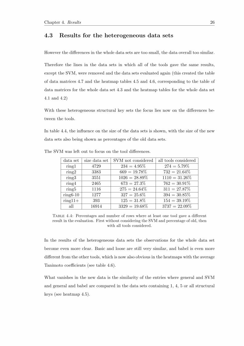
However the differences in the whole data sets are too small, the data overall too similar.

Therefore the lines in the data sets in which all of the tools gave the same results,

except the SVM, were removed and the data sets evaluated again (this created the table

of data matrices 4.7 and the heatmap tables 4.5 and 4.6, corresponding to the table of

data matrices for the whole data set 4.3 and the heatmap tables for the whole data set

4.1 and 4.2)

With these heterogeneous structural key sets the focus lies now on the differences be-

tween the tools.

In table 4.4, the influence on the size of the data sets is shown, with the size of the new

data sets also being shown as percentages of the old data sets.

The SVM was left out to focus on the tool differences.

data set size data set SVM not considered all tools considered

ring1 4729 234 = 4.95% 274 = 5.79%

ring2 3383 669 = 19.78% 732 = 21.64%

ring3 3551 1026 = 28.89% 1110 = 31.26%

ring4 2465 673 = 27.3% 762 = 30.91%

ring5 1116 275 = 24.64% 311 = 27.87%

ring6-10 1277 327 = 25.6% 394 = 30.85%

ring11+ 393 125 = 31.8% 154 = 39.19%

all 16914 3329 = 19.68% 3737 = 22.09%

Table 4.4: Percentages and number of rows where at least one tool gave a differentresult in the evaluation. First without considering the SVM and percentage of old, then

with all tools considered.

In the results of the heterogeneous data sets the observations for the whole data set

become even more clear. Basic and loose are still very similar, and babel is even more

different from the other tools, which is now also obvious in the heatmaps with the average

Tanimoto coefficients (see table 4.6).

What vanishes in the new data is the similarity of the entries where general and SVM

and general and babel are compared in the data sets containing 1, 4, 5 or all structural

keys (see heatmap 4.5).



bab bas gen loo

bas

gen

loo

svm

3

31.2

4.7

15

65.8

98.3

88

67.5

60.7 89.7


bab bas gen loo

bas

gen

loo

svm

0.9

40.4

0.6

18.4

55.6

99.7

67.3

55.3

28.3 67


bab bas gen loo

bas

gen

loo

svm

0.6

36.2

0.6

9.3

52.9

99.5

63.4

52.9

30 63.7


bab bas gen loo

bas

gen

loo

svm

0.9

18.1

0.9

20.2

67.6

100

48.3

67.6

32.7 48.3


bab bas gen loo

bas

gen

loo

svm

0

18.5

0

22.9

63.3

100

48.4

63.3

27.3 48.4

Percentages equal#rings: 6−10

bab bas gen loo

bas

gen

loo

svm

0.6

7.6

0

31.2

80.7

99.4

36.7

80.1

30.6 36.1

Percentages equal#rings: 11+

bab bas gen loo

bas

gen

loo

svm

2.4

3.2

1.6

25.6

88.8

99.2

62.4

88

53.6 61.6

Percentages equal#rings: all

bab bas gen loo

bas

gen

loo

svm

0.9

27.5

0.9

17.6

62.3

99.6

58.9

62.2

33.1 59

Table 4.5: Heatmaps of the percentage of equal structural keys, pairwise for eachtool. Heterogeneous data sets.



bab bas gen loo

bas

gen

loo

svm

0

0

0

0

0.4

0.8

0.7

0.5

0.4 0.7


bab bas gen loo

bas

gen

loo

svm

0.2

0.3

0.2

0.2

0.7

1

0.7

0.7

0.4 0.7


bab bas gen loo

bas

gen

loo

svm

0.3

0.4

0.3

0.4

0.7

1

0.7

0.7

0.5 0.7


bab bas gen loo

bas

gen

loo

svm

0.3

0.4

0.3

0.4

0.8

1

0.7

0.8

0.6 0.7


bab bas gen loo

bas

gen

loo

svm

0.4

0.5

0.4

0.5

0.8

1

0.7

0.8

0.6 0.7

Average Tanimoto#rings: 6−10

bab bas gen loo

bas

gen

loo

svm

0.4

0.5

0.4

0.6

0.9

1

0.7

0.9

0.6 0.7

Average Tanimoto#rings: 11+

bab bas gen loo

bas

gen

loo

svm

0.5

0.5

0.5

0.5

0.9

1

0.9

0.9

0.8 0.9

Average Tanimoto#rings: all

bab bas gen loo

bas

gen

loo

svm

0.3

0.4

0.3

0.4

0.7

1

0.7

0.7

0.5 0.7

Table 4.6: Heatmaps of the average Tanimoto coefficient of the structural keys, pair-wise for each tool. Heterogeneous data sets.












OpenBabel 0.89 18.13 0.89 20.21 OpenBabel 0.31 0.39 0.31 0.45basic NA 67.61 100 48.29 basic NA 0.8 1 0.69



OpenBabel 0 18.55 0 22.91 OpenBabel 0.41 0.46 0.41 0.54basic NA 63.27 100 48.36 basic NA 0.81 1 0.7


percentage ring 6-10 tanimoto ring 6-10basic general loose SVM basic general loose SVM

OpenBabel 0.61 7.65 0 31.19 OpenBabel 0.45 0.48 0.45 0.6basic NA 80.73 99.39 36.7 basic NA 0.9 1 0.68


percentage ring 11+ tanimoto ring 11+basic general loose SVM basic general loose SVM


general NA NA 88 53.6 general NA NA 0.93 0.81loose NA NA NA 61.6 loose NA NA NA 0.86

percentage whole data set tanimoto whole data setbasic general loose SVM basic general loose SVM



Table 4.7: Evaluation of the percentage of equal structural keys in the heterogeneousdata sets (each subtable), pairwise for each of the tools

Chapter 5

Discussion and conclusion

The main problem of aromaticity perception is the lack of a real definition. Because of

this most tools used nowadays are rule-based and do not agree with each other on all

molecules. The SVM can only be as good as the data it was trained on, therefore, when

used on the output of the tools, it can compensate the mistakes a tools makes with the

results the other tools give. It can also predict aromaticity for molecules the tools might

have no rules for.

In the testing phase of the SVM it correctly recognized 91.7% of the aromatic molecules

(see table 3.1). The averages of all results for each tool compared to all other tools,

except the SVM, should therefore be close to the similarity of this tool with the SVM.

These values are listed for in table 5.1 for the whole data sets and in table 5.2 for the

heterogeneous data sets. As one can see, the SVM works well for all of the tools. In

table 5.2 general and babel are less similar to the SVM than to all other tools, because

of the similarity of basic and loose. It influences the SVM to be more similar to each of

them, while the average of general and babel compared to each other tool contains the

comparison to both loose and basic.

The problem with the data collected in this thesis is that the loose and basic methods

turned out to give such similar results. This caused their predictions to weigh double. It

would have been desirable to train the SVM on the output of tools with a lot of different

results, so the disadvantages of each tool would be compensated better. For this reason

the training of the SVM should be done again, leaving out either the loose or the basic

tool.

30

Chapter 5. Discussion and conclusion 31

The data does however show that the SVM performs equally well as each of the tools,

slightly worse for the babel tool, since it is so different to the other tools. Given the

output of more tools with different methods as input it will be better at assigning aro-

maticity than all of them, since it can fully recover the knowledge used by the tools to

assign aromaticity [5] and combine it, such that the problems of each tool are compen-

sated.

If in the future a database is created that contains reliable aromaticity information, the

SVM would be the tool best suited for aromaticity perception.

percentages

tool a b

babel 82.24% 81.37%basic 91% 89.51%

general 90.29% 84.42%loose 90.99% 89.52%

tanimoto

tool a b

babel 0.65 0.65basic 0.72 0.72

general 0.71 0.68loose 0.72 0.72

Table 5.1: Whole data set, (a) Average of percentage result of each tool compared toall other tools (except the SVM) and (b) the results of the SVM compared to this tool

percentages

tool a b

babel 9.71% 17.6%basic 54.25% 58.94%

general 50.68% 33.07%loose 54.23% 59.03%

tanimoto

tool a b

babel 0.31 0.3721basic 0.6616 0.7097

general 0.6102 0.5331loose 0.6619 0.7102

Table 5.2: Whole heterogeneous data set, (a) Average of percentage result of eachtool compared to all other tools (except the SVM) and (b) the results of the SVM

compared to this tool

Bibliography

[1] Daylight depict. http://www.daylight.com/daycgi/depict. Accessed: July,

2013.

[2] Aromaticity wikipedia. http://en.wikipedia.org/wiki/Aromaticity, . Ac-

cessed: July, 2013.

[3] Pyrrole wikipedia. http://en.wikipedia.org/wiki/Pyrrole, . Accessed: August,

2013.

[4] ChemAxon. Aromaticity detection in marvin. http://www.chemaxon.com/

marvin/help/sci/aromatization-doc.html. Accessed: July, 2013.

[5] M. Mann, F. Costa, H. Ekke, C. Flamm, and R. Backofen. Data-driven aromatic

ring prediction with graph kernels, 2011.

[6] F. Costa and K. De Grave. Fast neighborhood subgraph pairwise distance kernel.

In Proc. of ICML, Haifa, pages 255–262, 2010.

[7] Martin Mann and Bernhard Thiel. Kekule structure enumeration yields unique

smiles, 2013.

[8] Amnon Stanger. What is... aromaticity: a critique of the concept of aromaticity-can

it really be defined? Chem. Commun., 0:1939–1947, 2009. doi: 10.1039/B816811C.

[9] H. Hart, L.E.Craine, and D.J.Hart. Organische Chemie. Wiley-VCH, 1999.

[10] G.M. Badger. Aromatic character and aromaticity. Cambridge Chemistry Texts,

1969.

[11] M. Mann, H. Ekker, P.F. Stadler, and C. Flamm. Atom mapping with con-

straint programming. In R. Backofen and S. Will, editors, Proceedings of the

32

http://www.daylight.com/daycgi/depict

http://en.wikipedia.org/wiki/Aromaticity

http://en.wikipedia.org/wiki/Pyrrole

http://www.chemaxon.com/marvin/help/sci/aromatization-doc.html

http://www.chemaxon.com/marvin/help/sci/aromatization-doc.html

Bibliography 33

Workshop on Constraint Based Methods for Bioinformatics WCB12, pages 23–

29, Freiburg, 2012. Uni Freiburg. http://www.bioinf.uni-freiburg.de/Events/

WCB12/proceedings.pdf.

[12] Smiles theory. http://www.daylight.com/dayhtml/doc/theory/theory.

finger.html. Accessed: July, 2013.

[13] The homepage of embl-ebi. available from http://www.ebi.ac.uk/chebi/

userManualForward.do#3-Star%20status. Accessed June, 2013.

[14] Chebi database. available from ftp://ftp.ebi.ac.uk/pub/databases/chebi/

SDF/ChEBI_complete_3star.sdf.gz, 2013. Accessed June, 2013.

[15] D. Weininger. SMILES, a chemical language and information system. 1. Introduc-

tion to methodology and encoding rules. J. Chem. Inf. Comp. Sci., 28(1):31–36,

1988. doi: 10.1021/ci00057a005.

[16] Martin Mann, Heinz Ekker, and Christoph Flamm. The graph grammar library - a

generic framework for chemical graph rewrite systems. In Keith Duddy and Gerti

Kappel, editors, Theory and Practice of Model Transformations, Proc. of ICMT

2013, volume 7909 of LNCS, pages 52–53. Springer, 2013. ISBN 978-3-642-38882-8.

doi: 10.1007/978-3-642-38883-5 5. Extended abstract and poster at ICMT, full

article at arXiv.

[17] Noel M O′Boyle, Michael Banck, Craig A James, Chris Morley, Tim Vandermeersch,

and Geoffrey R Hutchison. Open babel: An open chemical toolbox. Journal of

Cheminformatics, 3(1):33, 2011.

http://www.bioinf.uni-freiburg.de/Events/WCB12/proceedings.pdf

http://www.bioinf.uni-freiburg.de/Events/WCB12/proceedings.pdf

http://www.daylight.com/dayhtml/doc/theory/theory.finger.html

http://www.daylight.com/dayhtml/doc/theory/theory.finger.html

http://www.ebi.ac.uk/chebi/userManualForward.do#3-Star%20status

http://www.ebi.ac.uk/chebi/userManualForward.do#3-Star%20status

ftp://ftp.ebi.ac.uk/pub/databases/chebi/SDF/ChEBI_complete_3star.sdf.gz

ftp://ftp.ebi.ac.uk/pub/databases/chebi/SDF/ChEBI_complete_3star.sdf.gz

Selbststandigkeitserklarung

Hiermit erklare ich, dass ich diese Abschlussarbeit selbstandig verfasst habe, keine an-

deren als die angegebenen Quellen/Hilfsmittel verwendet habe und alle Stellen, die

wortlich oder sinngemaß aus veroffentlichten Schriften entnommen wurden, als solche

kenntlich gemacht habe. Daruber hinaus erklare ich, dass diese Abschluss-arbeit nicht,

auch nicht auszugsweise, bereits fur eine andere Prufung angefertigt wurde.

Ort, Datum:

Unterschrift:

34

Graph kernel based aromaticity predictionAbstract Aromaticity is an important property of molecules,...

Documents

Transcript of Graph kernel based aromaticity predictionAbstract Aromaticity is an important property of molecules,...