Graph Convolutions on Spectral Embeddingsfor Cortical Surface Parcellation

Karthik Gopinath1,⇤, Christian Desrosiers1, Herve Lombaert1

ETS Montreal, Canada

Abstract

Neuronal cell bodies mostly reside in the cerebral cortex. The study of this thin and highly convolutedsurface is essential for understanding how the brain works. The analysis of surface data is, however, challeng-ing due to the high variability of the cortical geometry. This paper presents a novel approach for learningand exploiting surface data directly across multiple surface domains. Current approaches rely on geometri-cal simplifications, such as spherical inflations, a popular but costly process. For instance, the widely usedFreeSurfer takes about 3 hours to parcellate brain surfaces on a standard machine. Direct learning of surfacedata via graph convolutions would provide a new family of fast algorithms for processing brain surfaces.However, the current limitation of existing state-of-the-art approaches is their inability to compare surfacedata across di↵erent surface domains. Surface bases are indeed incompatible between brain geometries. Thispaper leverages recent advances in spectral graph matching to transfer surface data across aligned spectraldomains. This novel approach enables direct learning of surface data across compatible surface bases. Itexploits spectral filters over intrinsic representations of surface neighborhoods. We illustrate the benefits ofthis approach with an application to brain parcellation. We validate the algorithm over 101 manually la-beled brain surfaces. The results show a significant improvement in labeling accuracy over recent Euclideanapproaches while gaining a drastic speed improvement over conventional methods.

Keywords: Graph Convolution Networks; Geometric Deep Learning; Spectral Graph Theory; CorticalParcellation

1. Introduction

Neuroimage analysis consists of studying functional and anatomical information over the brain geometry.Various aspects of the brain are investigated using di↵erent imaging modalities, such as magnetic resonanceimaging (MRI) data. Structural MRI provides notably the geometry of the cortex. The thin outer layerof the brain cerebrum is of particular interest due to its vital role in cognition, vision, and perception.5

Statistical frameworks on surfaces are, therefore, highly sought for studying various aspects of the brain.For instance, variations in surface data can reveal new biomarkers as well as possible relations with diseaseprocesses (Arbabshirani et al., 2017). The challenge consists of learning surface data over highly complexand convoluted surfaces and across di↵erent subjects across a datasets.

The goal of separating the cerebral cortex into distinct regions based on structure or function is known10

as parcellation. Initially, automated parcellation techniques used clustering based on local regional statistics(Craddock et al., 2012). For instance, a semi-supervised technique (Glasser et al., 2016) delineated thecortical boundary from sharp changes in multimodal MRI data. Most research works use a cortical surfacebased feature to find surface correspondence. BrainVisa (Cointepas et al., 2010; Riviere et al., 2003; Auziaset al., 2013) uses sulcal features defined by the cortical folding patterns to find correspondence between brain15

⇤Corresponding author: K. Gopinath, ETS Montreal, Computer and Software Engineering, 1100 Notre Dame St. W.,Montreal QC, H3C 1K3, Canada. Email: karthik.gopinath.1@etsmtl.net

Preprint submitted to Elsevier March 30, 2019

s

Spectral coordinates

Sulcal depth

eu•,1

eu•,2

eu•,3

...

Input Layer 1 Output

Spectral features

...

Layer 2

Spectral features

...

Layer L

Spectral features

Graph convolutions of spectral filters

Parcel probabilities

Final parcellation

. . .y(1)•,1 y(2)

•,1 y(L)•,1

y(1)•,M1

y(2)•,M2

y(L)•,ML

...p•,1

p•,C

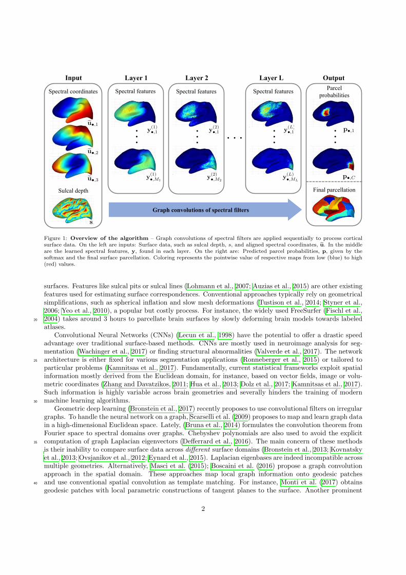
Figure 1: Overview of the algorithm – Graph convolutions of spectral filters are applied sequentially to process corticalsurface data. On the left are inputs: Surface data, such as sulcal depth, s, and aligned spectral coordinates, eu. In the middleare the learned spectral features, y, found in each layer. On the right are: Predicted parcel probabilities, p, given by thesoftmax and the final surface parcellation. Coloring represents the pointwise value of respective maps from low (blue) to high(red) values.

surfaces. Features like sulcal pits or sulcal lines (Lohmann et al., 2007; Auzias et al., 2015) are other existingfeatures used for estimating surface correspondences. Conventional approaches typically rely on geometricalsimplifications, such as spherical inflation and slow mesh deformations (Tustison et al., 2014; Styner et al.,2006; Yeo et al., 2010), a popular but costly process. For instance, the widely used FreeSurfer (Fischl et al.,2004) takes around 3 hours to parcellate brain surfaces by slowly deforming brain models towards labeled20

atlases.Convolutional Neural Networks (CNNs) (Lecun et al., 1998) have the potential to o↵er a drastic speed

advantage over traditional surface-based methods. CNNs are mostly used in neuroimage analysis for seg-mentation (Wachinger et al., 2017) or finding structural abnormalities (Valverde et al., 2017). The networkarchitecture is either fixed for various segmentation applications (Ronneberger et al., 2015) or tailored to25

particular problems (Kamnitsas et al., 2017). Fundamentally, current statistical frameworks exploit spatialinformation mostly derived from the Euclidean domain, for instance, based on vector fields, image or volu-metric coordinates (Zhang and Davatzikos, 2011; Hua et al., 2013; Dolz et al., 2017; Kamnitsas et al., 2017).Such information is highly variable across brain geometries and severally hinders the training of modernmachine learning algorithms.30

Geometric deep learning (Bronstein et al., 2017) recently proposes to use convolutional filters on irregulargraphs. To handle the neural network on a graph, Scarselli et al. (2009) proposes to map and learn graph datain a high-dimensional Euclidean space. Lately, (Bruna et al., 2014) formulates the convolution theorem fromFourier space to spectral domains over graphs. Chebyshev polynomials are also used to avoid the explicitcomputation of graph Laplacian eigenvectors (De↵errard et al., 2016). The main concern of these methods35

is their inability to compare surface data across di↵erent surface domains (Bronstein et al., 2013; Kovnatskyet al., 2013; Ovsjanikov et al., 2012; Eynard et al., 2015). Laplacian eigenbases are indeed incompatible acrossmultiple geometries. Alternatively, Masci et al. (2015); Boscaini et al. (2016) propose a graph convolutionapproach in the spatial domain. These approaches map local graph information onto geodesic patchesand use conventional spatial convolution as template matching. For instance, Monti et al. (2017) obtains40

geodesic patches with local parametric constructions of tangent planes to the surface. Another prominent

2

spatial approach Velickovic et al. (2018) proposes to include self-attentional layers in which neighborhoodsare used to avoid an explicit computation of a graph Laplacian. This attentional approach reduces toa particular formulation of Monti et al. (2017). A related work (Simonovsky and Komodakis, 2017) alsoconditions convolutional filter weights on specific edge labels over neighborhoods rather than on graph nodes.45

Applications of graph convolution networks in neuroimaging remain yet limited. Existing work includes theuse of graph convolutions over population graphs for predicting brain disorders and learning distance metricsin functional brain networks (Parisot et al., 2018; Ktena et al., 2017). A recent work (Cucurull et al., 2018)proposes to parcellate the cerebral cortex into three parcels using an attention-based method (Velickovicet al., 2018). Brain meshes are, however, constrained within a unique graph structure, limiting all meshes to50

use the same mesh geometry. Fundamentally, these methods either lack the capability to process multiplesurface domains (Bronstein et al., 2013; Kovnatsky et al., 2013; Ovsjanikov et al., 2012; Eynard et al.,2015) or have spatial representations of surface data defined in a Euclidean space, which ignore the complexgeometry of the surface. They rely, for instance, on polar representations of mesh vertices (Boscaini et al.,2016; Masci et al., 2015; Monti et al., 2017; Velickovic et al., 2018).55

This paper leverages recent advances in spectral graph matching to transfer surface data across alignedspectral domains (Lombaert et al., 2015a). The transfer of spectral coordinates across domains providesa robust formulation for spectral methods that naturally handles di↵erences across Laplacian eigenvectors,including sign flips, ordering, and mixing of eigenvectors in higher frequencies. This spectral alignmentstrategy was exploited to learn surface data (Lombaert et al., 2015b) within the random forest framework.60

Spectral Forests are operating in a spectral domain and use the first spectral coordinates as well as sulcaldepth of each cortical point. This approach is, however, limited to only pointwise information, ignoringlocal patterns within surface neighborhoods. Our approach consists of leveraging spectral coordinates withingraph convolutional networks to bridge a gap between learning algorithms and geometrical representations.To the best of our knowledge, this is the first attempt at intrinsically learning surface data via spectral65

graph convolutions in neuroimaging. This novel approach enables a direct learning of surface data acrosscompatible surface bases by exploiting spectral filters over intrinsic representations of surface neighborhoods.

The main contributions of our work are:

• A novel spectral graph convolutional approach for cortical parcellation,

• A direct learning of surface data using trainable spectral filters over surface embeddings,70

• The training of spectral filters across multiple mesh geometries of various graph structures,

• The leverage of spectral filters to exploit local patterns of data within surface neighborhoods,

• An evaluation on the largest publicly available dataset of manually labeled brain surfaces (Klein et al.,2017),

• An improved state-of-the-art performance for cortical surface parcellation with graph convolutions.75

In this work, we propose a surface learning algorithm. We illustrate the learning capabilities of this ap-proach with an application to brain parcellation. We choose cortical parcellation since it provides establishedbenchmarks with publicly available datasets of manual labelings. The validation over the largest publiclyavailable dataset of manually labeled brain surfaces (Klein et al., 2017), with 101 subjects, demonstratesa significant improvement in using spectral graph convolutions over Euclidean approaches. This change of80

paradigm indeed improves the parcellation accuracy when using graph convolutions, from a Dice score of53% to 85%. Our approach is at least at par with the well established FreeSurfer algorithm (Fischl et al.,2004) when benchmarking over a large dataset (Klein et al., 2017), while gaining a drastic speed improve-ment in the order of seconds. The next section details the fundamentals of our spectral approach, followedby experiments evaluating the impact of our spectral strategy over standard Euclidean approaches for graph85

convolutions.

3

Leaky ReLU

Spectral filterconvolution

Leaky ReLU

Leaky ReLU

Leaky ReLU

Spectral filterconvolution

Spectral filterconvolution

Spectral filterconvolution Softmax

M1 = 256

K1 = 6

M2 = 128

K2 = 6

M3 = 64

K3 = 6

M4 = 32

K4 = 6

N ⇥ 4 N ⇥ 32

OutputInput

KernelInputFilter weightsFeature map Bias

Convolution block

z(l)ip =X

j2Ni

MlX

q=1

KlX

k=1

w(l)pqk · y(l)jq · '(bui, buj ; µ

(l)k ,�(l)

k ) + b(l)p .

z(l)ip =X

j2Ni

MlX

q=1

KlX

k=1

w(l)pqk · y(l)jq · '(bui, buj ; µ

(l)k ,�(l)

k ) + b(l)p .

z(l)ip =X

j2Ni

MlX

q=1

KlX

k=1

w(l)pqk · y(l)jq · '(bui, buj ; µ

(l)k ,�(l)

k ) + b(l)p .z(l)ip =X

j2Ni

MlX

q=1

KlX

k=1

w(l)pqk · y(l)jq · '(bui, buj ; µ

(l)k ,�(l)

k ) + b(l)p .z(l)ip =X

j2Ni

MlX

q=1

KlX

k=1

w(l)pqk · y(l)jq · '(bui, buj ; µ

(l)k ,�(l)

k ) + b(l)p .

+⇥⇥

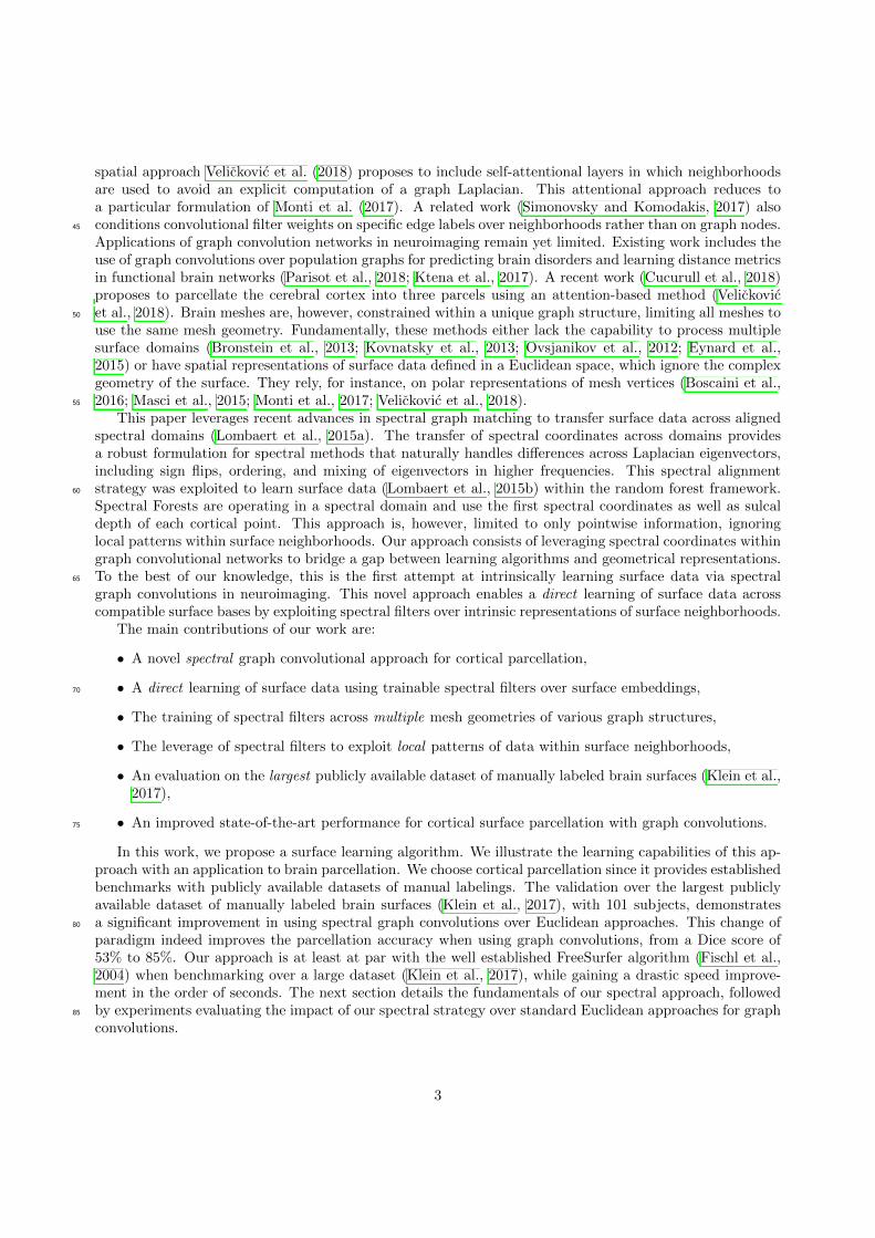
Figure 2: Overview of the network architecture – Dense connections are used among successive layers constituted withgraph convolutions of learned spectral filters and leaky ReLU activations. Weights (w), biases (b), and parameters of ourspectral filters (µ,�) are learned via back-propagation. A final softmax function produces parcel probabilities (p) on the brainsurface.

2. Method

An overview of the proposed method is shown in Fig. 1. In a first step, each cortical surface is modeledas a graph. Spectral decomposition is then applied on these graphs to capture the intrinsic geometry ofbrain surfaces and embed this information in a low-dimensional feature space (Lombaert et al., 2015a;90

Lefevre et al., 2018). Subsequently, the transfer of surface data between spectral embeddings enables graphconvolution networks to process cortical data across multiple mesh domains. This is implemented with arealignment of spectral embeddings. Finally, cortical parcellation is performed by learning spectral filtersover realigned spectral coordinates and cortical features like the sulcal depth. Dense connections (Huanget al., 2017) improve convergence by propagating information from the initial layers to output layers. We95

therefore use dense connections among successive graph convolution layers. The overview of the networkarchitecture is shown in Fig. 2.

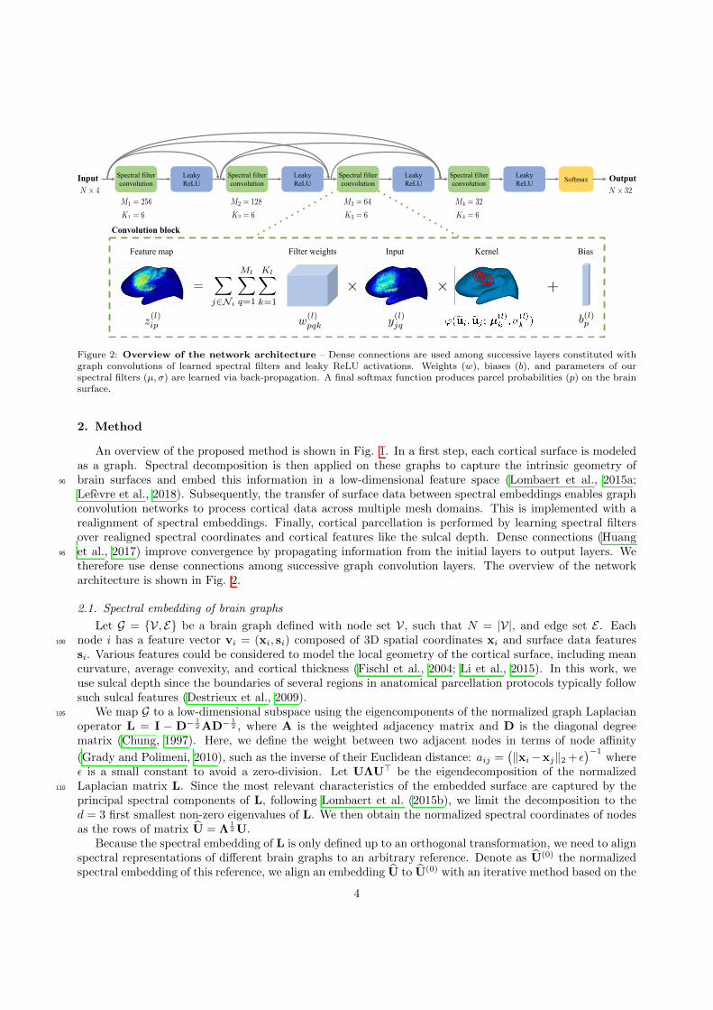
2.1. Spectral embedding of brain graphs

Let G = {V, E} be a brain graph defined with node set V, such that N = |V|, and edge set E . Eachnode i has a feature vector vi = (xi, si) composed of 3D spatial coordinates xi and surface data features100

si. Various features could be considered to model the local geometry of the cortical surface, including meancurvature, average convexity, and cortical thickness (Fischl et al., 2004; Li et al., 2015). In this work, weuse sulcal depth since the boundaries of several regions in anatomical parcellation protocols typically followsuch sulcal features (Destrieux et al., 2009).

We map G to a low-dimensional subspace using the eigencomponents of the normalized graph Laplacian105

operator L = I � D� 12 AD� 1

2 , where A is the weighted adjacency matrix and D is the diagonal degreematrix (Chung, 1997). Here, we define the weight between two adjacent nodes in terms of node a�nity

(Grady and Polimeni, 2010), such as the inverse of their Euclidean distance: aij =�kxi �xjk2 + ✏

��1where

✏ is a small constant to avoid a zero-division. Let U⇤U> be the eigendecomposition of the normalizedLaplacian matrix L. Since the most relevant characteristics of the embedded surface are captured by the110

principal spectral components of L, following Lombaert et al. (2015b), we limit the decomposition to thed = 3 first smallest non-zero eigenvalues of L. We then obtain the normalized spectral coordinates of nodesas the rows of matrix bU = ⇤

12 U.

Because the spectral embedding of L is only defined up to an orthogonal transformation, we need to alignspectral representations of di↵erent brain graphs to an arbitrary reference. Denote as bU(0) the normalizedspectral embedding of this reference, we align an embedding bU to bU(0) with an iterative method based on the

4

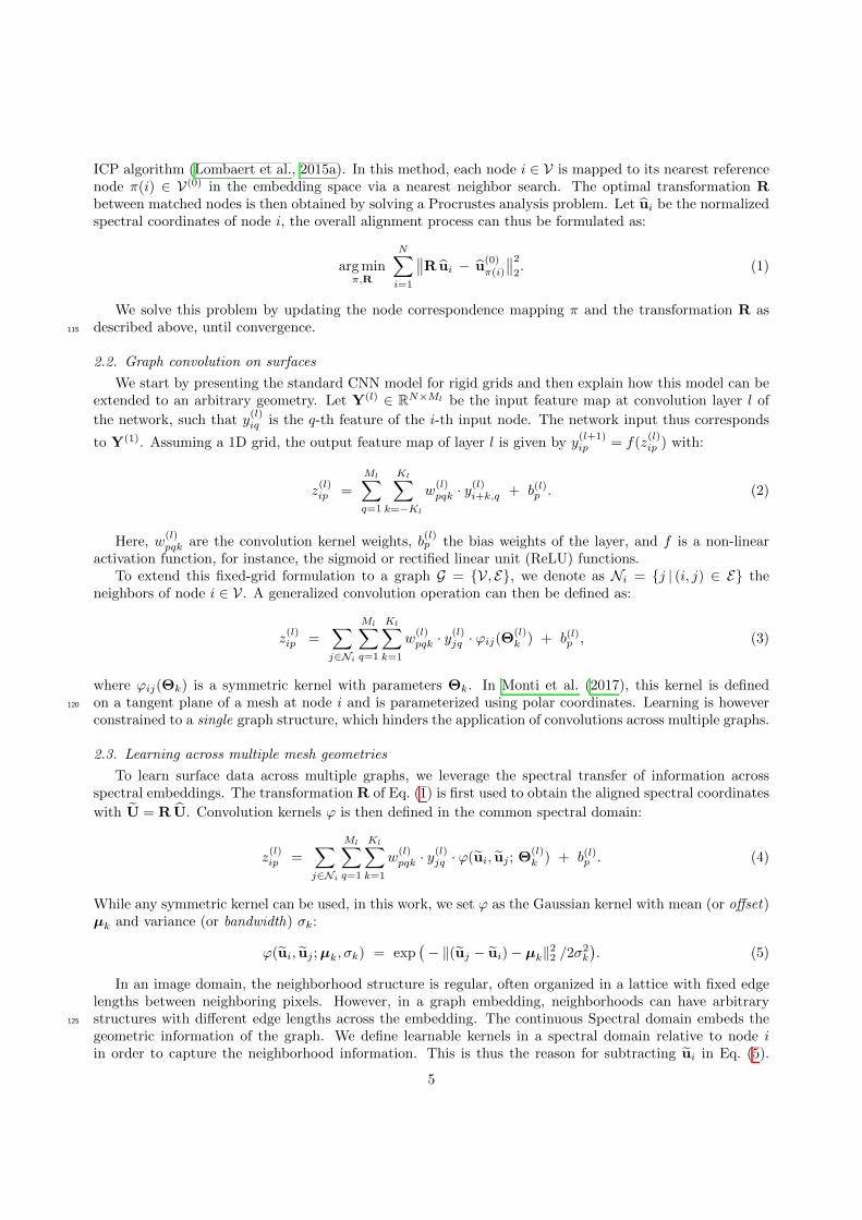
ICP algorithm (Lombaert et al., 2015a). In this method, each node i 2 V is mapped to its nearest referencenode ⇡(i) 2 V(0) in the embedding space via a nearest neighbor search. The optimal transformation Rbetween matched nodes is then obtained by solving a Procrustes analysis problem. Let bui be the normalizedspectral coordinates of node i, the overall alignment process can thus be formulated as:

arg min⇡,R

NX

i=1

��R bui � bu(0)⇡(i)

��2

2. (1)

We solve this problem by updating the node correspondence mapping ⇡ and the transformation R asdescribed above, until convergence.115

2.2. Graph convolution on surfaces

We start by presenting the standard CNN model for rigid grids and then explain how this model can beextended to an arbitrary geometry. Let Y(l) 2 RN⇥Ml be the input feature map at convolution layer l of

the network, such that y(l)iq is the q-th feature of the i-th input node. The network input thus corresponds

to Y(1). Assuming a 1D grid, the output feature map of layer l is given by y(l+1)ip = f(z(l)ip ) with:

z(l)ip =MlX

q=1

KlX

k=�Kl

w(l)pqk · y(l)

i+k,q + b(l)p . (2)

Here, w(l)pqk are the convolution kernel weights, b(l)p the bias weights of the layer, and f is a non-linear

activation function, for instance, the sigmoid or rectified linear unit (ReLU) functions.To extend this fixed-grid formulation to a graph G = {V, E}, we denote as Ni = {j | (i, j) 2 E} the

neighbors of node i 2 V. A generalized convolution operation can then be defined as:

z(l)ip =X

j2Ni

MlX

q=1

KlX

k=1

w(l)pqk · y(l)

jq · 'ij(⇥(l)k ) + b(l)p , (3)

where 'ij(⇥k) is a symmetric kernel with parameters ⇥k. In Monti et al. (2017), this kernel is definedon a tangent plane of a mesh at node i and is parameterized using polar coordinates. Learning is however120

constrained to a single graph structure, which hinders the application of convolutions across multiple graphs.

2.3. Learning across multiple mesh geometries

To learn surface data across multiple graphs, we leverage the spectral transfer of information acrossspectral embeddings. The transformation R of Eq. (1) is first used to obtain the aligned spectral coordinates

with eU = R bU. Convolution kernels ' is then defined in the common spectral domain:

z(l)ip =X

j2Ni

MlX

q=1

KlX

k=1

w(l)pqk · y(l)

jq · '(eui, euj ; ⇥(l)k ) + b(l)p . (4)

While any symmetric kernel can be used, in this work, we set ' as the Gaussian kernel with mean (or o↵set)µk and variance (or bandwidth) �k:

'(eui, euj ; µk, �k) = exp�� k(euj � eui) � µkk22 /2�2

k

�. (5)

In an image domain, the neighborhood structure is regular, often organized in a lattice with fixed edgelengths between neighboring pixels. However, in a graph embedding, neighborhoods can have arbitrarystructures with di↵erent edge lengths across the embedding. The continuous Spectral domain embeds the125

geometric information of the graph. We define learnable kernels in a spectral domain relative to node iin order to capture the neighborhood information. This is thus the reason for subtracting eui in Eq. (5).

5

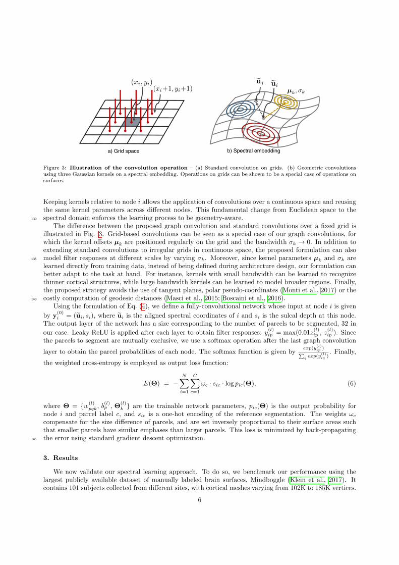
(xi, yi)(xi+1, yi+1)

a) Grid space

euieuj

µk, �k

b) Spectral embedding

Figure 3: Illustration of the convolution operation – (a) Standard convolution on grids. (b) Geometric convolutionsusing three Gaussian kernels on a spectral embedding. Operations on grids can be shown to be a special case of operations onsurfaces.

Keeping kernels relative to node i allows the application of convolutions over a continuous space and reusingthe same kernel parameters across di↵erent nodes. This fundamental change from Euclidean space to thespectral domain enforces the learning process to be geometry-aware.130

The di↵erence between the proposed graph convolution and standard convolutions over a fixed grid isillustrated in Fig. 3. Grid-based convolutions can be seen as a special case of our graph convolutions, forwhich the kernel o↵sets µk are positioned regularly on the grid and the bandwidth �k ! 0. In addition toextending standard convolutions to irregular grids in continuous space, the proposed formulation can alsomodel filter responses at di↵erent scales by varying �k. Moreover, since kernel parameters µk and �k are135

learned directly from training data, instead of being defined during architecture design, our formulation canbetter adapt to the task at hand. For instance, kernels with small bandwidth can be learned to recognizethinner cortical structures, while large bandwidth kernels can be learned to model broader regions. Finally,the proposed strategy avoids the use of tangent planes, polar pseudo-coordinates (Monti et al., 2017) or thecostly computation of geodesic distances (Masci et al., 2015; Boscaini et al., 2016).140

Using the formulation of Eq. (4), we define a fully-convolutional network whose input at node i is given

by y(0)i = (eui, si), where eui is the aligned spectral coordinates of i and si is the sulcal depth at this node.

The output layer of the network has a size corresponding to the number of parcels to be segmented, 32 in

our case. Leaky ReLU is applied after each layer to obtain filter responses: y(l)ip = max(0.01z(l)ip , z(l)ip ). Since

the parcels to segment are mutually exclusive, we use a softmax operation after the last graph convolution

layer to obtain the parcel probabilities of each node. The softmax function is given byexp(y(l)

ip )P

q exp(y(l)iq )

. Finally,

the weighted cross-entropy is employed as output loss function:

E(⇥) = �NX

i=1

CX

c=1

!c · sic · log pic(⇥), (6)

where ⇥ = {w(l)pqk, b(l)p , ⇥(l)

k } are the trainable network parameters, pic(⇥) is the output probability fornode i and parcel label c, and sic is a one-hot encoding of the reference segmentation. The weights !c

compensate for the size di↵erence of parcels, and are set inversely proportional to their surface areas suchthat smaller parcels have similar emphases than larger parcels. This loss is minimized by back-propagatingthe error using standard gradient descent optimization.145

3. Results

We now validate our spectral learning approach. To do so, we benchmark our performance using thelargest publicly available dataset of manually labeled brain surfaces, Mindboggle (Klein et al., 2017). Itcontains 101 subjects collected from di↵erent sites, with cortical meshes varying from 102K to 185K vertices.

6

1 2 3 4 5 6 7Number of kernels (K)

68707274767880828486

Dic

e ov

erla

p (%

)

L = 1L = 2L = 3L = 4

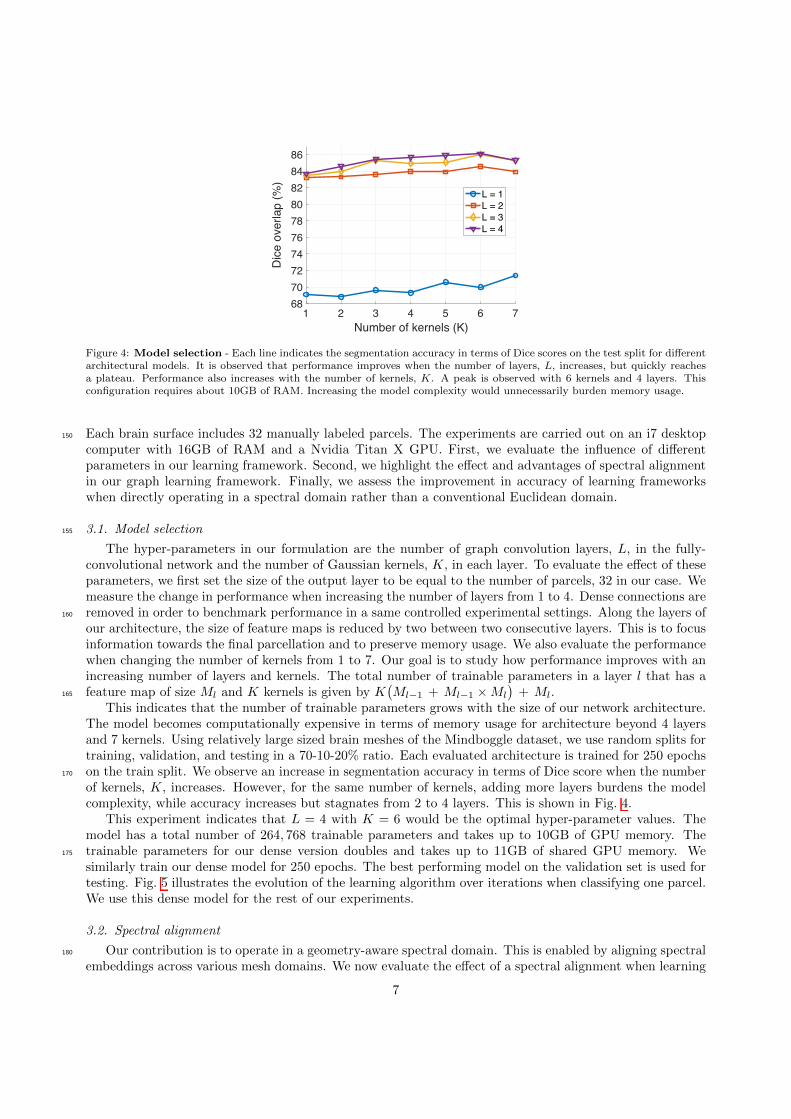
Figure 4: Model selection - Each line indicates the segmentation accuracy in terms of Dice scores on the test split for di↵erentarchitectural models. It is observed that performance improves when the number of layers, L, increases, but quickly reachesa plateau. Performance also increases with the number of kernels, K. A peak is observed with 6 kernels and 4 layers. Thisconfiguration requires about 10GB of RAM. Increasing the model complexity would unnecessarily burden memory usage.

Each brain surface includes 32 manually labeled parcels. The experiments are carried out on an i7 desktop150

computer with 16GB of RAM and a Nvidia Titan X GPU. First, we evaluate the influence of di↵erentparameters in our learning framework. Second, we highlight the e↵ect and advantages of spectral alignmentin our graph learning framework. Finally, we assess the improvement in accuracy of learning frameworkswhen directly operating in a spectral domain rather than a conventional Euclidean domain.

3.1. Model selection155

The hyper-parameters in our formulation are the number of graph convolution layers, L, in the fully-convolutional network and the number of Gaussian kernels, K, in each layer. To evaluate the e↵ect of theseparameters, we first set the size of the output layer to be equal to the number of parcels, 32 in our case. Wemeasure the change in performance when increasing the number of layers from 1 to 4. Dense connections areremoved in order to benchmark performance in a same controlled experimental settings. Along the layers of160

our architecture, the size of feature maps is reduced by two between two consecutive layers. This is to focusinformation towards the final parcellation and to preserve memory usage. We also evaluate the performancewhen changing the number of kernels from 1 to 7. Our goal is to study how performance improves with anincreasing number of layers and kernels. The total number of trainable parameters in a layer l that has afeature map of size Ml and K kernels is given by K

�Ml�1 + Ml�1 ⇥ Ml

�+ Ml.165

This indicates that the number of trainable parameters grows with the size of our network architecture.The model becomes computationally expensive in terms of memory usage for architecture beyond 4 layersand 7 kernels. Using relatively large sized brain meshes of the Mindboggle dataset, we use random splits fortraining, validation, and testing in a 70-10-20% ratio. Each evaluated architecture is trained for 250 epochson the train split. We observe an increase in segmentation accuracy in terms of Dice score when the number170

of kernels, K, increases. However, for the same number of kernels, adding more layers burdens the modelcomplexity, while accuracy increases but stagnates from 2 to 4 layers. This is shown in Fig. 4.

This experiment indicates that L = 4 with K = 6 would be the optimal hyper-parameter values. Themodel has a total number of 264, 768 trainable parameters and takes up to 10GB of GPU memory. Thetrainable parameters for our dense version doubles and takes up to 11GB of shared GPU memory. We175

similarly train our dense model for 250 epochs. The best performing model on the validation set is used fortesting. Fig. 5 illustrates the evolution of the learning algorithm over iterations when classifying one parcel.We use this dense model for the rest of our experiments.

3.2. Spectral alignment

Our contribution is to operate in a geometry-aware spectral domain. This is enabled by aligning spectral180

embeddings across various mesh domains. We now evaluate the e↵ect of a spectral alignment when learning

7

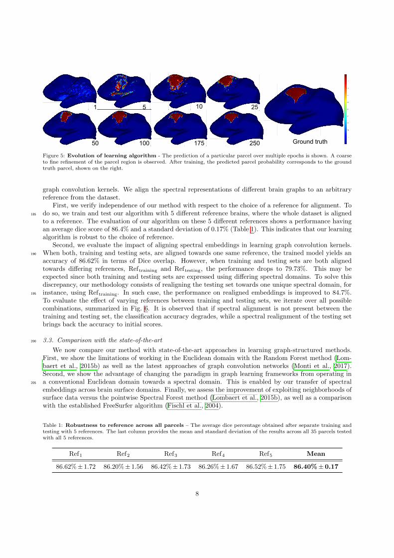
1 5 10 25

50 100 175 250 Ground truth

Figure 5: Evolution of learning algorithm - The prediction of a particular parcel over multiple epochs is shown. A coarseto fine refinement of the parcel region is observed. After training, the predicted parcel probability corresponds to the groundtruth parcel, shown on the right.

graph convolution kernels. We align the spectral representations of di↵erent brain graphs to an arbitraryreference from the dataset.

First, we verify independence of our method with respect to the choice of a reference for alignment. Todo so, we train and test our algorithm with 5 di↵erent reference brains, where the whole dataset is aligned185

to a reference. The evaluation of our algorithm on these 5 di↵erent references shows a performance havingan average dice score of 86.4% and a standard deviation of 0.17% (Table 1). This indicates that our learningalgorithm is robust to the choice of reference.

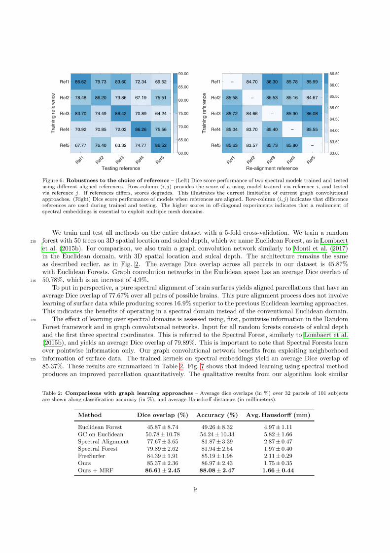
Second, we evaluate the impact of aligning spectral embeddings in learning graph convolution kernels.When both, training and testing sets, are aligned towards one same reference, the trained model yields an190

accuracy of 86.62% in terms of Dice overlap. However, when training and testing sets are both alignedtowards di↵ering references, Reftraining and Reftesting, the performance drops to 79.73%. This may beexpected since both training and testing sets are expressed using di↵ering spectral domains. To solve thisdiscrepancy, our methodology consists of realigning the testing set towards one unique spectral domain, forinstance, using Reftraining. In such case, the performance on realigned embeddings is improved to 84.7%.195

To evaluate the e↵ect of varying references between training and testing sets, we iterate over all possiblecombinations, summarized in Fig. 6. It is observed that if spectral alignment is not present between thetraining and testing set, the classification accuracy degrades, while a spectral realignment of the testing setbrings back the accuracy to initial scores.

3.3. Comparison with the state-of-the-art200

We now compare our method with state-of-the-art approaches in learning graph-structured methods.First, we show the limitations of working in the Euclidean domain with the Random Forest method (Lom-baert et al., 2015b) as well as the latest approaches of graph convolution networks (Monti et al., 2017).Second, we show the advantage of changing the paradigm in graph learning frameworks from operating ina conventional Euclidean domain towards a spectral domain. This is enabled by our transfer of spectral205

embeddings across brain surface domains. Finally, we assess the improvement of exploiting neighborhoods ofsurface data versus the pointwise Spectral Forest method (Lombaert et al., 2015b), as well as a comparisonwith the established FreeSurfer algorithm (Fischl et al., 2004).

Table 1: Robustness to reference across all parcels – The average dice percentage obtained after separate training andtesting with 5 references. The last column provides the mean and standard deviation of the results across all 35 parcels testedwith all 5 references.

Ref1 Ref2 Ref3 Ref4 Ref5 Mean

86.62%± 1.72 86.20%± 1.56 86.42%± 1.73 86.26%± 1.67 86.52%± 1.75 86.40%± 0.17

8

86.62

78.48

83.70

70.92

67.77

79.73

86.20

74.49

70.85

76.40

83.60

73.86

86.42

72.02

63.32

72.34

67.19

70.89

86.26

74.77

69.52

75.51

64.24

75.56

86.52

Ref1 Ref2 Ref3 Ref4 Ref5

Testing reference

Ref1

Ref2

Ref3

Ref4

Ref5

Trai

ning

refe

renc

e

60.00

65.00

70.00

75.00

80.00

85.00

90.00

85.58

85.72

85.04

85.63

84.70

84.66

83.70

83.57

86.30

85.53

85.40

85.73

85.78

85.16

85.90

85.80

85.99

84.67

86.08

85.55

Ref1 Ref2 Ref3 Ref4 Ref5

Re-alignment reference

Ref1

Ref2

Ref3

Ref4

Ref5

Trai

ning

refe

renc

e

83.00

83.50

84.00

84.50

85.00

85.50

86.00

86.50

Figure 6: Robustness to the choice of reference – (Left) Dice score performance of two spectral models trained and testedusing di↵erent aligned references. Row-column (i, j) provides the score of a using model trained via reference i, and testedvia reference j. If references di↵ers, scores degrades. This illustrates the current limitation of current graph convolutionalapproaches. (Right) Dice score performance of models when references are aligned. Row-column (i, j) indicates that di↵erencereferences are used during trained and testing. The higher scores in o↵-diagonal experiments indicates that a realinment ofspectral embeddings is essential to exploit multiple mesh domains.

We train and test all methods on the entire dataset with a 5-fold cross-validation. We train a randomforest with 50 trees on 3D spatial location and sulcal depth, which we name Euclidean Forest, as in Lombaert210

et al. (2015b). For comparison, we also train a graph convolution network similarly to Monti et al. (2017)in the Euclidean domain, with 3D spatial location and sulcal depth. The architecture remains the sameas described earlier, as in Fig. 2. The average Dice overlap across all parcels in our dataset is 45.87%with Euclidean Forests. Graph convolution networks in the Euclidean space has an average Dice overlap of50.78%, which is an increase of 4.9%.215

To put in perspective, a pure spectral alignment of brain surfaces yields aligned parcellations that have anaverage Dice overlap of 77.67% over all pairs of possible brains. This pure alignment process does not involvelearning of surface data while producing scores 16.9% superior to the previous Euclidean learning approaches.This indicates the benefits of operating in a spectral domain instead of the conventional Euclidean domain.

The e↵ect of learning over spectral domains is assessed using, first, pointwise information in the Random220

Forest framework and in graph convolutional networks. Input for all random forests consists of sulcal depthand the first three spectral coordinates. This is referred to the Spectral Forest, similarly to Lombaert et al.(2015b), and yields an average Dice overlap of 79.89%. This is important to note that Spectral Forests learnover pointwise information only. Our graph convolutional network benefits from exploiting neighborhoodinformation of surface data. The trained kernels on spectral embeddings yield an average Dice overlap of225

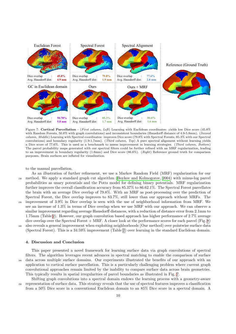
85.37%. These results are summarized in Table 2. Fig. 7 shows that indeed learning using spectral methodproduces an improved parcellation quantitatively. The qualitative results from our algorithm look similar

Table 2: Comparisons with graph learning approaches – Average dice overlaps (in %) over 32 parcels of 101 subjectsare shown along classification accuracy (in %), and average Hausdor↵ distances (in millimeters).

Method Dice overlap (%) Accuracy (%) Avg.Hausdor↵ (mm)

Euclidean Forest 45.87± 8.74 49.26± 8.32 4.97± 1.11

GC on Euclidean 50.78± 10.78 54.24± 10.33 5.82± 1.66

Spectral Alignment 77.67± 3.65 81.87± 3.39 2.87± 0.47

Spectral Forest 79.89± 2.62 81.94± 2.54 1.97± 0.40

FreeSurfer 84.39± 1.91 85.19± 1.98 2.11± 0.29

Ours 85.37± 2.36 86.97± 2.43 1.75± 0.35

Ours + MRF 86.61± 2.45 88.08± 2.47 1.66± 0.44

9

Euclidean Forest

Ours Ours + MRF

Reference (Ground Truth)

GC in Euclidean domain

Spectral Forest Spectral Alignment

Dice overlap : 79.8%Avg. Hausdorff dist: 1.9 mm

Dice overlap : 77.6%Avg. Hausdorff dist: 2.8 mm

Dice overlap : 50.78%Avg. Hausdorff dist: 5.8 mm

Dice overlap : 85.3%Avg. Hausdorff dist: 1.7 mm

Dice overlap : 86.6%Avg. Hausdorff dist: 1.6 mm

Dice overlap : 45.8%Avg. Hausdorff dist: 4.9 mm

Figure 7: Cortical Parcellation – (First column, Left) Learning with Euclidean coordinates: yields low Dice score (45.8%with Random Forests, 50.8% with graph convolutions) and inconsistent boundaries (Hausdor↵ distance of 4.9-5.8mm). (Secondcolumn, Middle) Learning with Spectral coordinates: improves Dice score (79.8% with Spectral Forests, 85.3% with our Spectralconvolutions) and boundary regularity (1.9-1.7mm). (Third column, Top) A pure spectral alignment without learning yieldsa Dice score of 77.6%. This is used as a benchmark to assess improvement in learning strategies. (Third column, Bottom)The parcel probability maps generated with our spectral filters could be further refined with an MRF regularization, leadingto an improvement in boundary regularity (1.6mm) and Dice score (86.6%). (Right) Reference ground truth for comparisonpurposes. Brain surfaces are inflated for visualization.

to the manual parcellation.As an illustration of further refinement, we use a Markov Random Field (MRF) regularization for our

method. We apply a standard graph cut algorithm (Boykov and Kolmogorov, 2004) with minus-log parcel230

probabilities as unary potentials and the Potts model for defining binary potentials. MRF regularizationfurther improves the overall classification accuracy from 85.37% to 86.62.1%. The Spectral Forest parcellatesthe brain with an average Dice overlap of 79.8%. With an MRF as post-processing over the prediction ofSpectral Forest, the Dice overlap improves to 83.7%, still lower than our approach without MRFs. Theimprovement of 3.9% in Dice overlap is seen with the use of neighborhood information from MRF. We235

see an increase of 1.3% in terms of Dice overlap when we use MRF with our approach. We can observe asimilar improvement regarding average Hausdor↵ distances, with a reduction of distance error from 2.1mm to1.75mm (Table 2). However, our graph convolution based approach has higher performance of 2.7% averagedice overlap over the Spectral Forest + MRF. A closer look at the performance scores for each parcel (Fig. 8)also reveals a general improvement when exploiting neighborhoods (Our method) over pointwise surface data240

(Spectral Forest). This is a 34.59% improvement (Table 2) over learning in the standard Euclidean domain.

4. Discussion and Conclusion

This paper presented a novel framework for learning surface data via graph convolutions of spectralfilters. The algorithm leverages recent advances in spectral matching to enable the comparison of surfacedata across multiple surface domains. Our experiments illustrated the benefits of our approach with an245

application to cortical surface parcellation. This is a particularly challenging problem where current graphconvolutional approaches remain limited by the inability to compare surface data across brain geometries.This typically results in spatial irregularities of parcel boundaries as illustrated in Fig. 7.

Shifting graph convolutions into a spectral domain endows the learning process with a geometry-awarerepresentation of surface data. This strategy reveals that the use of spectral features improves a classification250

from a 50% Dice score in a conventional Euclidean domain to an 85% Dice score in a spectral domain. A

10

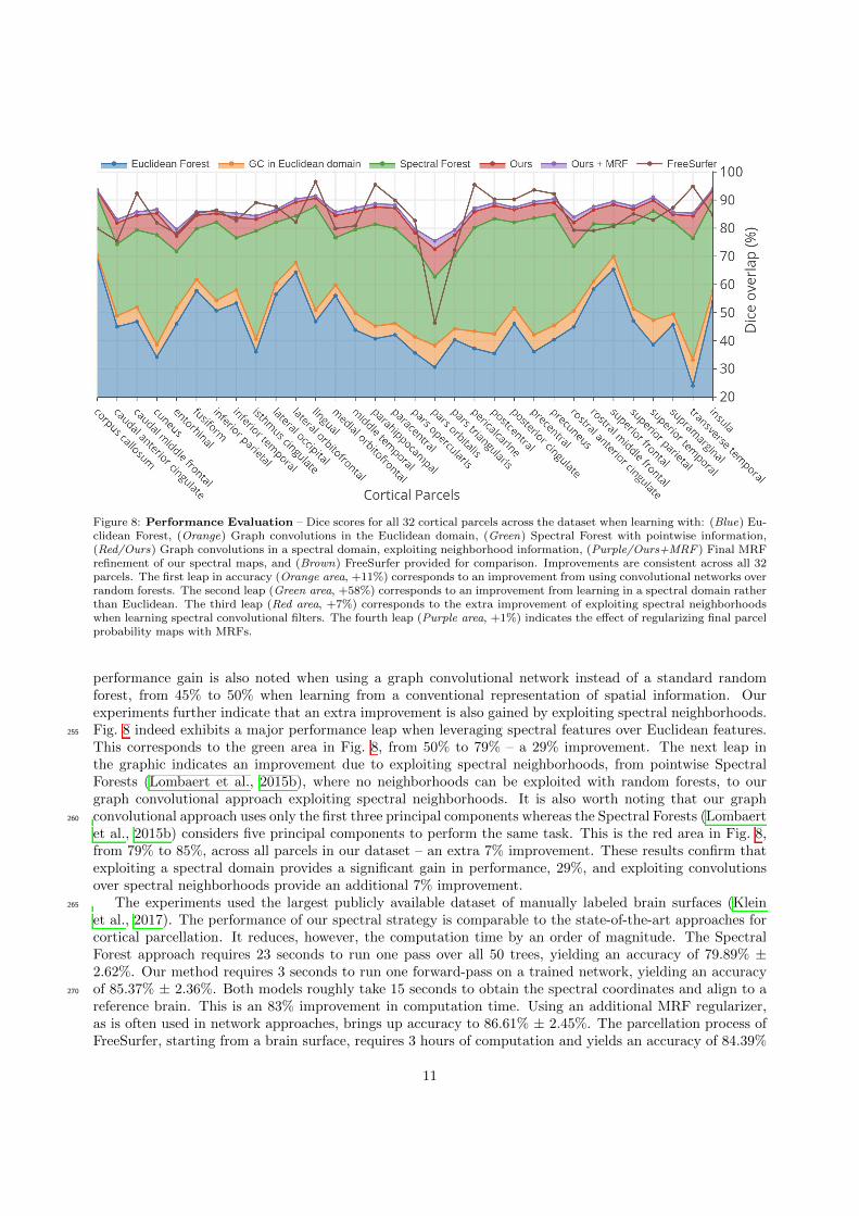
Figure 8: Performance Evaluation – Dice scores for all 32 cortical parcels across the dataset when learning with: (Blue) Eu-clidean Forest, (Orange) Graph convolutions in the Euclidean domain, (Green) Spectral Forest with pointwise information,(Red/Ours) Graph convolutions in a spectral domain, exploiting neighborhood information, (Purple/Ours+MRF ) Final MRFrefinement of our spectral maps, and (Brown) FreeSurfer provided for comparison. Improvements are consistent across all 32parcels. The first leap in accuracy (Orange area, +11%) corresponds to an improvement from using convolutional networks overrandom forests. The second leap (Green area, +58%) corresponds to an improvement from learning in a spectral domain ratherthan Euclidean. The third leap (Red area, +7%) corresponds to the extra improvement of exploiting spectral neighborhoodswhen learning spectral convolutional filters. The fourth leap (Purple area, +1%) indicates the e↵ect of regularizing final parcelprobability maps with MRFs.

performance gain is also noted when using a graph convolutional network instead of a standard randomforest, from 45% to 50% when learning from a conventional representation of spatial information. Ourexperiments further indicate that an extra improvement is also gained by exploiting spectral neighborhoods.Fig. 8 indeed exhibits a major performance leap when leveraging spectral features over Euclidean features.255

This corresponds to the green area in Fig. 8, from 50% to 79% – a 29% improvement. The next leap inthe graphic indicates an improvement due to exploiting spectral neighborhoods, from pointwise SpectralForests (Lombaert et al., 2015b), where no neighborhoods can be exploited with random forests, to ourgraph convolutional approach exploiting spectral neighborhoods. It is also worth noting that our graphconvolutional approach uses only the first three principal components whereas the Spectral Forests (Lombaert260

et al., 2015b) considers five principal components to perform the same task. This is the red area in Fig. 8,from 79% to 85%, across all parcels in our dataset – an extra 7% improvement. These results confirm thatexploiting a spectral domain provides a significant gain in performance, 29%, and exploiting convolutionsover spectral neighborhoods provide an additional 7% improvement.

The experiments used the largest publicly available dataset of manually labeled brain surfaces (Klein265

et al., 2017). The performance of our spectral strategy is comparable to the state-of-the-art approaches forcortical parcellation. It reduces, however, the computation time by an order of magnitude. The SpectralForest approach requires 23 seconds to run one pass over all 50 trees, yielding an accuracy of 79.89% ±2.62%. Our method requires 3 seconds to run one forward-pass on a trained network, yielding an accuracyof 85.37% ± 2.36%. Both models roughly take 15 seconds to obtain the spectral coordinates and align to a270

reference brain. This is an 83% improvement in computation time. Using an additional MRF regularizer,as is often used in network approaches, brings up accuracy to 86.61% ± 2.45%. The parcellation process ofFreeSurfer, starting from a brain surface, requires 3 hours of computation and yields an accuracy of 84.39%

11

± 1.91%. It is to be also noted that in the protocol of the Mindboggle dataset, annotations by experts are,in e↵ect, manual corrections from FreeSurfer parcellations (Klein et al., 2017). This creates a positive bias275

for FreeSurfer results. Our claim in our experiments is not necessarily a superiority of our approach, but torather provide a parcellation accuracy that is at least equivalent to FreeSurfer.

The advantage of using a spectral method is, on one hand, computational, by providing parcellation inseconds rather than hours, and on the other, methodological, by opening up a new learning strategy for pro-cessing cortical surface data. The technical contribution leveraged recent work on transfer of spectral bases280

across brain surface domains (Lombaert et al., 2015a,b). This enables the learning of spectral convolutionfilters across multiple brain geometries. This overcomes a major limitation in current graph convolutionalapproaches (Monti et al., 2017; Boscaini et al., 2016; Masci et al., 2015; Velickovic et al., 2018), whichare restrained to a unique fixed graph structure. Our method ameliorates graph spectral approaches byexploiting transfers of spectral bases. Furthermore, our experiments also used a multi-centric, multi-data285

and publicly available dataset. This provides an exhaustive, reproducible, evaluation for directly exploitingspectral features.

While the potential of our method is demonstrated on cortical parcellation, it can be applied to otheranalyses of surface data. For instance, our framework has a direct impact on regression problems that involvepredictions of cortical thickness over time, potentially leading to new families of geometry-based biomarkers290

for neurological disorders.

Acknowledgements

This work was supported financially by the Natural Sciences and Engineering Research Council of Canada(NSERC). We also gratefully acknowledge the support of NVIDIA Corporation with the donation of aTitan X GPU used for this research.295

References

Arbabshirani, M.R., Plis, S., Sui, J., Calhoun, V.D., 2017. Single subject prediction of brain disorders in neuroimaging:Promises and pitfalls. NeuroImage 145, 137–165.

Auzias, G., Brun, L., Deruelle, C., Coulon, O., 2015. Deep sulcal landmarks: Algorithmic and conceptual improvements in thedefinition and extraction of sulcal pits. Neuroimage 111, 12–25.300

Auzias, G., Lefevre, J., Le Troter, A., Fischer, C., Perrot, M., Regis, J., Coulon, O., 2013. Model-driven harmonic parameter-ization of the cortical surface: Hip-hop. IEEE transactions on medical imaging 32, 873–887.

Boscaini, D., Masci, J., Rodola, E., Bronstein, M., 2016. Learning shape correspondence with anisotropic convolutional neuralnetworks, in: NIPS, pp. 3189–3197.

Boykov, Y., Kolmogorov, V., 2004. An experimental comparison of min-cut/max-flow algorithms for energy minimization in305

vision. IEEE Transactions on PAMI 26, 1124–1137.Bronstein, M., Bruna, J., LeCun, Y., Szlam, A., Vandergheynst, P., 2017. Geometric deep learning: Going beyond Euclidean

data. IEEE Transactions on Signal Processing 34, 18–42.Bronstein, M., Glasho↵, K., Loring, T., 2013. Making Laplacians commute. arXiv:1307.6549.Bruna, J., Zaremba, W., Szlam, A., Lecun, Y., 2014. Spectral networks and locally connected networks on graphs, in: ICLR.310

Chung, F., 1997. Spectral Graph Theory. AMS.Cointepas, Y., Ge↵roy, D., Souedet, N., Denghien, I., Riviere, D., 2010. The BrainVISA project: a shared software development

infrastructure for biomedical imaging research. HBM 16.Craddock, R.C., James, G.A., Holtzheimer III, P.E., Hu, X.P., Mayberg, H.S., 2012. A whole brain fMRI atlas generated via

spatially constrained spectral clustering. Human brain mapping 33, 1914–1928.315

Cucurull, G., Wagstyl, K., Casanova, A., Velickovic, P., Jakobsen, E., Drozdzal, M., Romero, A., Evans, A., Bengio, Y., 2018.Convolutional neural networks for mesh-based parcellation of the cerebral cortex, in: MIDL, p. 1.

De↵errard, M., Bresson, X., Vandergheynst, P., 2016. Convolutional neural networks on graphs with fast localized spectralfiltering, in: NIPS, pp. 3844–3852.

Destrieux, C., Fischl, B., Dale, A., Halgren, E., 2009. A sulcal depth-based anatomical parcellation of the cerebral cortex.320

NeuroImage 47, 151–163.Dolz, J., Desrosiers, C., Ben Ayed, I., 2017. 3D fully convolutional networks for subcortical segmentation in MRI: A large-scale

study. NeuroImage 170, 456–470.Eynard, D., Kovnatsky, A., Bronstein, M.M., Glasho↵, K., Bronstein, A.M., 2015. Multimodal manifold analysis by simulta-

neous diagonalization of Laplacians. IEEE Transactions on PAMI 12, 2505–2517.325

12

Fischl, B., van der Kouwe, A., Destrieux, C., Halgren, E., Segonne, F., Salat, D.H., Busa, E., Seidman, L.J., Goldstein, J.,Kennedy, D., Caviness, V., Makris, N., Rosen, B., Dale, A.M., 2004. Automatically parcellating the human cerebral cortex.Cerebral cortex 14, 11–22.

Glasser, M.F., Coalson, T.S., Robinson, E.C., Hacker, C.D., Harwell, J., Yacoub, E., Ugurbil, K., Andersson, J., Beckmann,C.F., Jenkinson, M., et al., 2016. A multi-modal parcellation of human cerebral cortex. Nature 536, 171–178.330

Grady, L., Polimeni, J.R., 2010. Discrete Calculus: Applied Analysis on Graphs for Computational Science. Springer.Hua, X., Hibar, D.P., Ching, C.R., Boyle, C.P., Rajagopalan, P., Gutman, B.A., Leow, A.D., Toga, A.W., Jack, C.R.,

Harvey, D., Weiner, M.W., Thompson, P.M., Alzheimer’s Disease Neuroimaging Initiative, 2013. Unbiased tensor-basedmorphometry: Improved robustness and sample size estimates for Alzheimer’s disease clinical trials. NeuroImage 66, 648–661.335

Huang, G., Liu, Z., van der Maaten, L., Weinberger, K.Q., 2017. Densely connected convolutional networks, in: CVPR.Kamnitsas, K., Ledig, C., Newcombe, V.F.J., Simpson, J.P., Kane, A.D., Menon, D.K., Rueckert, D., Glocker, B., 2017.

E�cient multi-scale 3D CNN with fully connected CRF for accurate brain lesion segmentation. Medical Image Analysis 36,61–78.

Klein, A., Ghosh, S.S., Bao, F.S., Giard, J., Hame, Y., Stavsky, E., Lee, N., Rossa, B., Reuter, M., Chaibub Neto, E., Keshavan,340

A., 2017. Mindboggling morphometry of human brains. PLOS Computational Biology 13, e1005350.Kovnatsky, A., Bronstein, M.M., Bronstein, A.M., Glasho↵, K., Kimmel, R., 2013. Coupled quasi-harmonic bases, in: Computer

Graphics Forum, pp. 439–448.Ktena, S.I., Parisot, S., Ferrante, E., Rajchl, M., Lee, M., Glocker, B., Rueckert, D., 2017. Distance metric learning using

graph convolutional networks: Application to functional brain networks, in: MICCAI, pp. 469–477.345

Lecun, Y., Bottou, L., Bengio, Y., Ha↵ner, P., 1998. Gradient-based learning applied to document recognition. IEEE IntelligentSignal Processing 86, 2278–2324.

Lefevre, J., Pepe, A., Muscato, J., De Guio, F., Girard, N., Auzias, G., Germanaud, D., 2018. SPANOL (SPectral ANalysisof lobes): A spectral clustering framework for individual and group parcellation of cortical surfaces in lobes. Frontiers inNeuroscience 12, 354–366.350

Li, G., Wang, L., Shi, F., Gilmore, J.H., Lin, W., Shen, D., 2015. Construction of 4D high-definition cortical surface atlases ofinfants: Methods and applications. Medical Image Analysis 25, 22–36.

Lohmann, G., Von Cramon, D.Y., Colchester, A.C., 2007. Deep sulcal landmarks provide an organizing framework for humancortical folding. Cerebral Cortex 18, 1415–1420.

Lombaert, H., Arcaro, M., Ayache, N., 2015a. Brain transfer: Spectral analysis of cortical surfaces and functional maps, in:355

IPMI, pp. 474–487.Lombaert, H., Criminisi, A., Ayache, N., 2015b. Spectral forests: Learning of surface data, application to cortical parcellation,

in: MICCAI, pp. 547–555.Masci, J., Boscaini, D., Bronstein, M., Vandergheynst, P., 2015. Geodesic convolutional neural networks on Riemannian

manifolds, in: ICCV-3dRR, pp. 37–45.360

Monti, F., Boscaini, D., Masci, J., Rodola, E., Svoboda, J., Bronstein, M.M., 2017. Geometric deep learning on graphs andmanifolds using mixture model CNNs, in: CVPR, pp. 1–10.

Ovsjanikov, M., Ben-Chen, M., Solomon, J., Butscher, A., Guibas, L., 2012. Functional maps: A flexible representation ofmaps between shapes, in: SIGGRAPH, p. 30.

Parisot, S., Ktena, S.I., Ferrante, E., Lee, M., Guerrero, R., Glocker, B., Rueckert, D., 2018. Disease prediction using graph365

convolutional networks: Application to autism spectrum disorder and Alzheimers disease. Medical Image Analysis 48,117–130.

Riviere, D., Regis, J., Cointepas, Y., Papadopoulos-Orfanos, D., Cachia, A., Mangin, J.F., 2003. A freely available Anatomist-BrainVISA package for structural morphometry of the cortical sulci. Neuroimage 19, 934.

Ronneberger, O., Fischer, P., Brox, T., 2015. U-net: Convolutional networks for biomedical image segmentation, in: MICCAI,370

pp. 234–241.Scarselli, F., Gori, M., Tsoi, A.C., Hagenbuchner, M., Monfardini, G., 2009. The graph neural network model. IEEE Transac-

tions on Neural Networks 20, 61–80.Simonovsky, M., Komodakis, N., 2017. Dynamic edge-conditioned filters in convolutional neural networks on graphs, in: CVPR,

pp. 29–38.375

Styner, M., Oguz, I., Xu, S., Brechbuhler, C., Pantazis, D., Levitt, J.J., Shenton, M.E., Gerig, G., 2006. Framework for thestatistical shape analysis of brain structures using SPHARM-PDM. Insight journal 1071, 242–250.

Tustison, N.J., Cook, P.A., Klein, A., Song, G., Das, S.R., Duda, J.T., Kandel, B.M., van Strien, N., Stone, J.R., Gee,J.C., Avants, B.B., 2014. Large-scale evaluation of ANTs and FreeSurfer cortical thickness measurements. NeuroImage 99,166–179.380

Valverde, S., Cabezas, M., Roura, E., Gonzalez-Villa, S., Pareto, D., Vilanova, J.C., Ramio-Torrenta, L., Rovira, A., Oliver,A., Llado, X., 2017. Improving automated multiple sclerosis lesion segmentation with a cascaded 3D convolutional neuralnetwork approach. NeuroImage 155, 159–168.

Velickovic, P., Cucurull, G., Casanova, A., Romero, A., Lio, P., Bengio, Y., 2018. Graph attention networks, in: ICLR, p. 1.Wachinger, C., Reuter, M., Klein, T., 2017. DeepNAT: Deep convolutional neural network for segmenting neuroanatomy.385

NeuroImage 170, 434–445.Yeo, B.T., Sabuncu, M.R., Vercauteren, T., Ayache, N., Fischl, B., Golland, P., 2010. Spherical demons: Fast di↵eomorphic

landmark-free surface registration. IEEE Transactions on Medical Imaging 29, 650–668.Zhang, T., Davatzikos, C., 2011. ODVBA: Optimally-discriminative voxel-based analysis. IEEE Transactions on Medical

Imaging 30, 1441–1454.390

13