Graph Analytics Through Fine-Grained Parallelism

Zechao Shang†, Feifei Li‡, Jeffrey Xu Yu†, Zhiwei Zhang§, Hong Cheng††The Chinese University of Hong Kong, ‡University of Utah, §Hong Kong Baptist University

{zcshang,yu,hcheng}@se.cuhk.edu.hk, lifeifei@cs.utah.edu,cszwzhang@comp.hkbu.edu.hk

ABSTRACTLarge graphs are getting increasingly popular and even indispens-able in many applications, for example, in social media data, largenetworks, and knowledge bases. Efficient graph analytics thus be-comes an important subject of study. To increase efficiency andscalability, in-memory computation and parallelism have been ex-plored extensively to speed up various graph analytical workloads.In many graph analytical engines (e.g., Pregel, Neo4j, GraphLab),parallelism is achieved via one of the three concurrency controlmodels, namely, bulk synchronization processing (BSP), asynchronousprocessing, and synchronous processing. Among them, synchronousprocessing has the potential to achieve the best performance dueto fine-grained parallelism, while ensuring the correctness and theconvergence of the computation, if an effective concurrency con-trol scheme is used. This paper explores the topological propertiesof the underlying graph to design and implement a highly effec-tive concurrency control scheme for efficient synchronous process-ing in an in-memory graph analytical engine. Our design uses anovel hybrid approach that combines 2PL (two-phase locking) withOCC (optimistic concurrency control), for high degree and low de-gree vertices in a graph respectively. Our results show that theproposed hybrid synchronous scheduler has significantly outper-formed other synchronous schedulers in existing graph analyticalengines, as well as BSP and asynchronous schedulers.

1. INTRODUCTIONGraph is a perfect model to represent complex relationships among

objects, in particular, data interconnectivity and topology informa-tion. As a result, the graph data model has been used extensivelyto store, query, and analyze data from a number of important appli-cation domains ranging from social media data to large computeror transportation networks to knowledge bases (semantic web) andto biological structures [1, 17]. Large amounts of graph data andmany applications running on top drive the needs for efficient andscalable graph analytics.

To increase both efficiency and scalability, in-memory computa-tion and parallelism have been explored extensively as two veryuseful techniques to speed up analytics over large graphs. Inspired

Permission to make digital or hard copies of all or part of this work for personal orclassroom use is granted without fee provided that copies are not made or distributedfor profit or commercial advantage and that copies bear this notice and the full cita-tion on the first page. Copyrights for components of this work owned by others thanACM must be honored. Abstracting with credit is permitted. To copy otherwise, or re-publish, to post on servers or to redistribute to lists, requires prior specific permissionand/or a fee. Request permissions from permissions@acm.org.

SIGMOD’16, June 26-July 01, 2016, San Francisco, CA, USAc© 2016 ACM. ISBN 978-1-4503-3531-7/16/06. . . $15.00

DOI: http://dx.doi.org/10.1145/2882903.2915238

by the design and success of early systems like Pregel [35], mostgraph systems support the vertex-centric data model and program-ming paradigm, in which a graph is represented by a set of verticesand their edge lists. An edge list for a vertex v simply stores allneighboring vertices of v in the graph. A typical analytical work-load over a vertex-centric graph model can often be represented asfollows (suppose the graph has N vertices and UDF is some userdefined function):

for iteration i = 1...n // in iterationfor j = 1...N // all vertices

UDF(vj, edgeListj)

For example, the classic PageRank algorithm is an instantiationof the above computation framework. We often speed up this com-putation through parallelism, and existing graph systems have useddifferent consistency models for such parallelism. The most popu-lar choices are the following three consistency models, namely, thebulk synchronous parallel (BSP), asynchronous, and synchronousparallel processing. A major difference among these models istheir message passing mechanism and the staleness of messages.

BSP proceeds in iterations (or super-steps), and message pass-ing takes place at the end of an iteration, therefore the messagestaleness is exactly one iteration. AP may introduce a delay (ofuncertain length) in delivering messages. In contrast, in SP pro-cessing, a worker (thread) receives messages without any degree ofstaleness. In other words, the implication is that workers in the BSPmodel reach synchronized states at the end of an iteration, but theywill proceed with asynchronized states in the asynchronous model,and they have to wait for synchronization and only proceed whena synchronized state is obtained in the synchronous model. In thecontext of vertex-centric analytics, data consistency model decideswhether vertices are able to access up-to-date and consistent datavalues from other vertices during the computation.

BSP is the most popular model in practice due to its simplicity;it is adopted by the general parallel computing frameworks suchas MapReduce [8], Spark [66], and graph analytical systems suchas GraphX [64] that is based on Spark. Systems and programmingframeworks using the asynchronous model, including PowerGraph,Galois, Grace [15, 45, 59], were also proposed. The synchronousmodel was explored by a few existing systems (e.g., in GraphLab[33]), however, the overhead in ensuring synchronization needs tobe carefully addressed to avoid introducing significant negative im-pacts to system efficiency.

Ideally, no message staleness is the most desirable design sinceit leads to synchronized states for all workers in a parallel compu-tation framework. However, ensuring this in a synchronous modelis not trivial and waiting for synchronization may introduce signif-icant overheads in a system. In practice, the BSP and asynchronousmodels address this issue by exploring the trade-off between mes-

sage staleness and efficiency. In particular, the BSP model limits themassage staleness by introducing a barrier in its computation, i.e.,workers need to wait for the completion of the last thread from thecurrent iteration, which ensures that the states of different workersare synchronized by the end of each iteration. However, it suffersfrom the infamous straggler problem.

The asynchronous model, on the other hand, removes the re-striction of synchronization altogether, hence, can be very efficient.However, since asynchronous message might be significantly de-layed in reaching its target, which could lead to incorrect or un-stable computations. For many graph analytical workloads, the al-gorithms can recover the correct, synchronized states in next iter-ation. However, this is not the case for all analytics, and there arealgorithms that do not have an implementation that will eventuallyconverge using the asynchronous model. Even algorithms on con-vex problems which always leads to the correct answer may fallinto local minimum caused by the chaos of asynchrony, e.g., SGD(stochastic gradient descent) may fail to converge [69, 42].

Our contributions. In light of these limitations, we focus on im-proving the efficiency and scalability of parallel graph analytics us-ing synchronous parallel processing. We assume an in-memorycomputing engine, to focus on the effects of the concurrency con-trol model and eliminate the impacts of disk I/Os. We encapsu-late the computations initiated by each vertex in a given round as atransaction. Using this view, the synchronous computation is madeof transactions. Each transaction is an atomic unit of operations.By ensuring conflict serializability among these transactions, theresults of the concurrent execution of these transactions are equiva-lent to the results from a sequential execution of these transactions.The synchronous model eliminates unbounded latency in commu-nication and relieves developers from reasoning and debugging anon-deterministic system as that in the asynchronous model.

That said, we can use a standard concurrency control scheme,such as strict 2PL (two phase locking) or OCC (optimistic concur-rency control) to ensure the concurrent execution of these transac-tions. We define the degree of a vertex v as the number of edgesconnected to v. An important observation is that the distributionfor degrees of vertices in a graph has a strong influence on the like-lihood of having a transaction conflict. This observation explainswhy traditional schedulers such as 2PL or OCC lead to bad per-formance for graph analytics using the synchronous model. In par-ticular, degrees of vertices in a graph often follow a very skeweddistribution. This means that the locking-based approaches suchas 2PL will often lead to high locking overhead, while the non-locking based scheduler such as OCC will suffer from high abortrates at the time of transaction commit.

Inspired by this observation, we propose HSync, a hybrid sched-uler that combines both locking-based and non-locking based sched-ulers, to achieve high performance graph analytics through syn-chronous parallel processing. HSync adapts to a scale-free graphwhere the degrees of vertices may vary: it uses a locking-basedscheduler for high degree vertices, and a non-locking-based sched-uler for low degree vertices. This design ensures that transactionsfor high degree vertices will never need to abort due to low de-gree ones (which is important since it is expensive to abort thesetransactions). But transactions for low degree vertices may need toabort, however, they are not expensive, and doing so ensures thatalmost no deadlocks will ever occur as transactions for low degreevertices will never block the execution and commit of a high degreevertex’s transaction. Extensive experimental results confirmed thesuperior performance of our hybrid scheduler over existing sched-ulers for the synchronous model. They also show that by using our

hybrid scheduler, the synchronous model will outperform the asyn-chronous and BSP models for in-memory parallel graph analytics.

Organization: In Section 2, we formalize the vertex-centric paral-lel programming and computing framework, and compare differenttask schedulers and data consistency models in this framework. InSection 3, we formalize and describe synchronous parallel process-ing for fine-grained parallelism in graph analytics. In Section 4, wediscuss the impact of large scale-free graphs on synchronous paral-lel processing for graph analytics. In particular, we identify that theskew distribution for degrees of vertices in a graph is the root causefor the poor performance of existing schedulers. In Section 5, wepropose our hybrid scheduler HSync that uses the locking-basedapproach and the non-locking based scheme for high-degree andlow-degree graph vertices respectively. We show our experimentalresults in Section 6 and discuss the related work in Section 7. Thepaper is concluded in Section 8.

2. BACKGROUND AND FORMULATIONAs introduced in Section 1, we focus on in-memory graph an-

alytics. We assume that the graph data is owned and used by asingle user for each analytical workload, which is fairly commonin in-memory analytical systems, e.g, in Spark [66], GraphX [64],GraphLab [33], and many other graph analytical systems. A simpleway to generalize to multiple users is to make a copy of the under-lying graph for the execution of each analytical workload. We alsoassume that the graph data is static during the execution of an ana-lytical workload, i.e., there are no updates to the graph during theexecution of a graph analytics job. A user submits an analytical joband expects the exact results at the end of task completion. Reduc-ing the wall-clock processing time is the main objective.

We also assume that the data resides in memory during the en-tire execution. We make this assumption for two reasons. First, in-memory computing is increasingly common [67], and many graphdata does fit in memory. For example, as reported in [52], the me-dian size of data used in Yahoo’s and Microsoft’s analytics jobsis 14GB. On the other hand, memory capacity increases quicklyand it is not uncommon for many desktop machines nowadays tohave memory in tens of GB, and commercial multi-core serverscan support up to 6TB of memory.1 Moreover, high speed networkand RDMA (remote direct memory access) significantly reduce thelatency of remote memory accessing and the speed of accessingmemory in a remote node is close to the speed of accessing localmemory. Therefore, with the help of middleware like FARM andRAMCloud [11, 46], even really large data can still reside entirelyin memory over a cluster. Secondly, the focus of our work is to ana-lyze the impacts of concurrency control schedulers for synchronousparallel processing in graph analytics. Thus, we would like to elim-inate the impacts by other factors such as disk I/Os and highlightthe bottlenecks introduced by the concurrency model.

2.1 Vertex-Centric Parallel ComputingMost graph analytical systems, like Pregel [35], GraphLab [33],

and GraphX [64], are built based on the vertex centric (VC) model.In this model, user implements a user-defined function (UDF), whichis executed on each vertex iteratively as shown in Section 1.

The vertex-centric computing model can be made to run in paral-lel, which leads to vertex centric parallel programming and comput-ing. We illustrate a simplified framework of vertex centric parallelprogramming and computing in Fig. 1. The system consists of mul-tiple workers (computer nodes and/or cores). Each worker executesthe UDF on a vertex through the coordination of the task scheduler.1For example, Dell R920 by November 2015

Shared Memory

Consistency Control

Core 0 Core n

UDF

Task Scheduler

Frontend

...

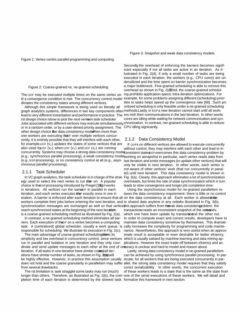
Figure 1: Vertex-centric parallel programming and computing.

barrier vertex

(a) BSP (b) straggler (c) fine-grain (d) barrier overhead

(e) barrier elimination

Figure 2: Coarse-grained vs. fine-grained scheduling

The UDF may be executed multiple times on the same vertex un-til a convergence condition is met. The concurrency control modeldictates the consistency states among different vertices.

Although this simple framework is being used on literally allgraph analytics systems, differences in two key components oftenlead to very different instantiation and performance in practice. Thefirst design choice is how to pick the next vertex v in task scheduler.Jobs associated with different vertices may execute simultaneously,or in a random order, or by a user-defined priority assignment. Theother design choice is the data consistency model: when more thanone workers are executing the UDF over multiple vertices concur-rently, it is entirely possible that they will interfere with each other,for example, UDF (v1) updates the states of some vertices that arealso used by UDF (v2) when UDF (v1) and UDF (v2) are runningconcurrently. Systems may choose a strong data consistency model(e.g., synchronous parallel processing), a weak consistency model(e.g., BSP processing), or no consistency control at all (e.g., asyn-chronous parallel processing).

2.1.1 Task SchedulerIn VC graph analytics, the task scheduler is in charge of the strat-

egy used to select the next vertex to run the UDF on. A popularchoice is the BSP processing introduced by Pregel [35]. BSP worksin iterations. All vertices run the same UDF in parallel in eachiteration, and each vertex executes the UDF exactly once in one it-eration. A barrier is enforced after each iteration to ensure that allworkers complete their jobs before entering the next iteration, andsynchronization messages are exchanged as well so that verticesreach synchronized states at the beginning of the next iteration. BSPis a coarse-grained scheduling method as illustrated by Fig. 2(a).

In contrast, a fine-grained scheduling method eliminates all bar-riers. Each execution of the UDF on a vertex becomes a computingtask. A (centralized) global scheduler, usually a work queue, isresponsible for scheduling. We illustrate its execution in Fig. 2(c).

The main advantage of coarse-grained scheduling like BSP is itssimplicity and low overhead in concurrency control, since verticesrun in parallel and isolation in one iteration and they only coor-dinate and send update messages to each other at the end of oneiteration. If all tasks in one iteration have similar costs, and all iter-ations have similar number of tasks, as shown in Fig. 2(a), BSP willbe highly effective. However, in practice this assumption usuallydoes not hold and the coarse granularity in parallelism may sufferfrom several drawbacks.

The first limitation is task straggler: some tasks may run (much)longer than others. Therefore, as illustrated as Fig. 2(b), the com-pletion time of each iteration is determined by the slowest task.

vertex read writeUDF

u

v

w

barrier

(a) Snapshot consistency (b) Weak consistency

Figure 3: Snapshot and weak data consistency models.

Secondly, the overhead of enforcing the barriers becomes signif-icant especially if not all tasks are active in an iteration. As il-lustrated in Fig. 2(d), if only a small number of tasks are beingexecuted in each iteration, the workers (e.g., CPU cores) are un-derutilized and the time spent on barrier synchronization becomesa major bottleneck. Fine-grained scheduling is able to remove thisoverhead as shown in Fig. 2(e). Third, the coarse-grained schedul-ing prohibits application-specific intra-iteration optimizations. Forexample, for some problems assigning different (scheduling) prior-ities to tasks helps speed up the convergence rate [68]. Such pri-oritized scheduling is only feasible under a fine-grained schedulingmethods. Lastly, in BSP a new iteration cannot start until all work-ers finish their communications in the last iteration. In other wordscores are idling while waiting for network communication and syn-chronization. In contrast, finer-grained scheduling is able to reduceCPU idling significantly.

2.1.2 Data Consistency ModelIf UDFs on different vertices are allowed to execute concurrently

without control, they may interfere with each other and lead to in-consistent states. BSP overcomes this data consistency problem byworking on a snapshot. In particular, each vertex reads data fromlast iteration and emits messages (to update other vertices) that willonly be visible in next iteration. In other words, each vertex isnot aware of other vertices’ work (that run concurrently in paral-lel) until next iteration. This data consistency model is shown inFig. 3(a). Clearly, this approach eliminates a lot of synchronizationoverheads, but limits the rate of state synchronization which in turnleads to slow convergence and longer job completion time.

Using the asynchronous model for fine-grained parallelism re-laxes the data consistency requirement: there is little or no controlon the data consistency at all. Each worker is allowed to writeto shared data anytime in any order. As illustrated in Fig. 3(b),this approach suffers from the weak data consistency problem: thetransaction w reads an inconsistent snapshot of the vertex u and v,which one have been update by transaction u and the other not.In order to compute exact and correct results, developers have tomaintain data consistency somehow by themselves. This dramati-cally increases the complexity for programming and code mainte-nance. Nevertheless, this approach is very useful when an approx-imate result is acceptable or even desirable for better efficiency,which is usually satisfied by machine learning and data mining ap-plications. However the exact trade-off between efficiency and ac-curacy is unclear and hard to model and reason about.

Lastly, strong data consistency model in fine-grained parallelismcan be achieved by using synchronous parallel processing. In par-ticular, for all workers that are being executed concurrently in par-allel, the strong data consistency model requires that they satisfyconflict serializability. In other words, the concurrent executionof these workers leads to a state that is the same as the state fromone of the serial executions of these workers. We will detail andformalize this framework in next section.

3. SYNCHRONOUS PARALLEL PROCESS-ING FOR FINE-GRAINED PARALLELISM

In this section we propose the fine-grained parallelism for graphanalytics with strong data consistency by using synchronous par-allel processing. Following the general VC framework, user willsubmit an UDF and it is executed over vertices in a graph. UDF (vj)may read other vertices’ attribute values and write values back. Thetask scheduler consists of the following modules:

1) The class vertex models the actions related to a vertex. Itasks for an implementation of the UDF for this vertex, that may becalled multiple times and may have different actions in each exe-cution depending on the current states of the vertices in a graph. Italso provides the interfaces for reading and writing values from andto other vertices. vertex can access its edge lists. For simplic-ity we do not distinguish the direction of edges. Instead we modelthem as undirected ones with tags. In other words, a vertex ob-ject represents a task related to a specific vertex.

2) addTask adds a task into the scheduler’s queue, possiblywith a priority assignment. Each task is removed from the sched-uler’s queue before its execution.

3) barrier introduces a global barrier; all workers enter thisbarrier after completing its currently assigned task. And they willexecute a user-specified function f before leaving the barrier. Thebarrier can be used for synchronization. The function f may useaddTask to add more tasks back to the queue. For example,to implement BSP-style scheduling, user adds each vertex usingaddTask and imposes the barrier based on a global value for itera-tion that is only updated when all workers in the current round havecompleted. Tasks in the next iteration are added back to the queueusing f . barrier is also used for progress monitoring, checkingfor termination condition, debugging and profiling, etc.

1 // global functions and class2 class vertex {3 abstract UDF(vertex v);4 value_t readVertex(vertex v);5 writeVertex(vertex v, value_t val);}6

7 addTask(vertex v, priority = 1.0);8 barrier(function f);

Figure 4: The API of fine-grained parallelism.1 in parallel for each worker (executed by a

thread)2 if at barrier3 wait until all workers reach barrier4 execute the function f5 continue6 if no more tasks in the scheduler queue7 exit8 retrieve (and remove) task vertex v9 begin transaction

10 execute UDF(v) as a transaction t(v)11 end transaction

Figure 5: The workflow of fine-grained parallelism.The workflow of fine-grained parallelism is shown as Fig. 5.

Once a worker becomes available, it retrieves a task from the sched-uler and executes the task concurrently in parallel with other activeworkers while ensuring strong data consistency. The UDF is treatedas an atomic unit. Atomic units run concurrently, but each of thembehaves like running by its own in isolation. Although users can de-fine such atomic unit with arbitrary logic, the most common form ingraph analytics involves computations over a single vertex and itsneighbors and the edges between them if applicable (i.e., its edgelist). These computations form an atomic unit and are encapsulatedby the UDF. Each such UDF proceeds as long as it does not interfere(i.e., conflict with) other concurrently running UDFs. For example,a conflict is identified if UDF (v1) tries to update the attribute values

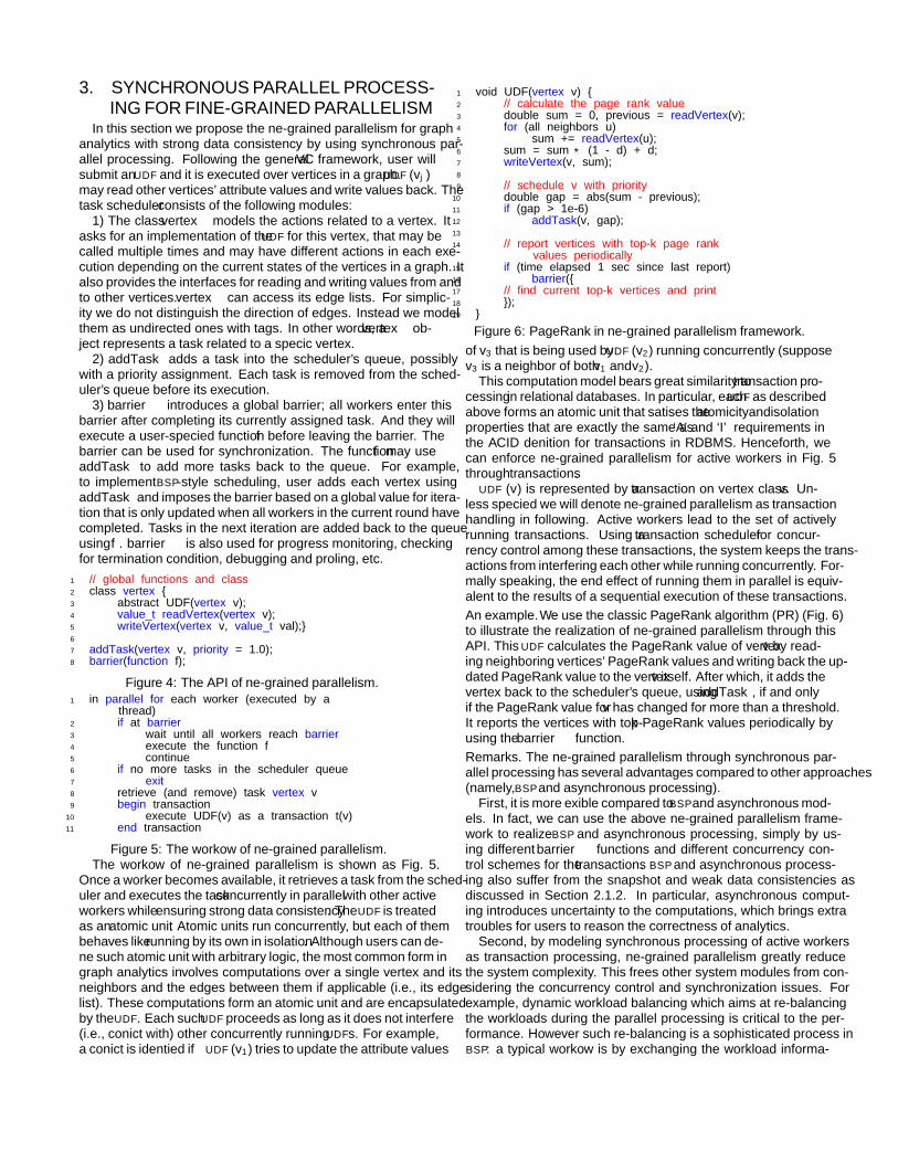
1 void UDF(vertex v) {2 // calculate the page rank value3 double sum = 0, previous = readVertex(v);4 for (all neighbors u)5 sum += readVertex(u);6 sum = sum * (1 - d) + d;7 writeVertex(v, sum);8

9 // schedule v with priority10 double gap = abs(sum - previous);11 if (gap > 1e-6)12 addTask(v, gap);13

14 // report vertices with top-k page rankvalues periodically

15 if (time elapsed 1 sec since last report)16 barrier({17 // find current top-k vertices and print18 });19 }

Figure 6: PageRank in fine-grained parallelism framework.of v3 that is being used by UDF (v2) running concurrently (supposev3 is a neighbor of both v1 and v2).

This computation model bears great similarity to transaction pro-cessing in relational databases. In particular, each UDF as describedabove forms an atomic unit that satisfies the atomicity and isolationproperties that are exactly the same as ‘A’ and ‘I’ requirements inthe ACID definition for transactions in RDBMS. Henceforth, wecan enforce fine-grained parallelism for active workers in Fig. 5through transactions.

UDF (v) is represented by a transaction on vertex class v. Un-less specified we will denote fine-grained parallelism as transactionhandling in following. Active workers lead to the set of activelyrunning transactions. Using a transaction scheduler for concur-rency control among these transactions, the system keeps the trans-actions from interfering each other while running concurrently. For-mally speaking, the end effect of running them in parallel is equiv-alent to the results of a sequential execution of these transactions.An example. We use the classic PageRank algorithm (PR) (Fig. 6)to illustrate the realization of fine-grained parallelism through thisAPI. This UDF calculates the PageRank value of vertex v by read-ing neighboring vertices’ PageRank values and writing back the up-dated PageRank value to the vertex v itself. After which, it adds thevertex back to the scheduler’s queue, using addTask, if and onlyif the PageRank value for v has changed for more than a threshold.It reports the vertices with top-k PageRank values periodically byusing the barrier function.Remarks. The fine-grained parallelism through synchronous par-allel processing has several advantages compared to other approaches(namely, BSP and asynchronous processing).

First, it is more flexible compared to BSP and asynchronous mod-els. In fact, we can use the above fine-grained parallelism frame-work to realize BSP and asynchronous processing, simply by us-ing different barrier functions and different concurrency con-trol schemes for the transactions. BSP and asynchronous process-ing also suffer from the snapshot and weak data consistencies asdiscussed in Section 2.1.2. In particular, asynchronous comput-ing introduces uncertainty to the computations, which brings extratroubles for users to reason the correctness of analytics.

Second, by modeling synchronous processing of active workersas transaction processing, fine-grained parallelism greatly reducethe system complexity. This frees other system modules from con-sidering the concurrency control and synchronization issues. Forexample, dynamic workload balancing which aims at re-balancingthe workloads during the parallel processing is critical to the per-formance. However such re-balancing is a sophisticated process inBSP: a typical workflow is by exchanging the workload informa-

tion several times before each worker agrees with the workloadsto be migrated. Additional communications are needed to performthe migration and notification [54, 23, 65]. Such complexity aredue to the staleness introduced by the coarse grain parallelism. Forfine-grained parallelism re-balancing is much simpler: underloadedworkers can steal the work from overloaded ones on the fly.

Lastly, dissemination of states among vertices is faster and syn-chronization reaches other vertices much quicker than using BSP,and ensures correctness that might not be possible in asynchronousmodel. For algorithms on convex problems like stochastic gradientdescent (SGD), the flexibility of fine-grained parallelism makes itpossible to support arbitrary update orders. Some gradients mayget updated more frequently than others, and these updates are in-stantly visible to others once the transactions commit. Thereforethe algorithm may converge faster. Non-convex and/or discreteproblems may have problem-specific constrains or dependencieson the update orders. Consider graph coloring as an example: eachvertex shall find a color distinct from its neighboring colors. It isimportant to ensure a vertex can access up-to-date and consistentcolor values of its neighbors during the computation. Fine-grainedparallelism helps enforce such constraints: user program does nothave to worry about a vertex u’s neighbors concurrently alter theircolors and lead to incorrect coloring assignment. Instead, the sys-tem itself will take over the concurrent executions while ensuringisolation. In contrast, the BSP model will incur significant over-head, and the asynchronous model may not even be able to imple-ment this correctly because each vertex cannot be sure to read itsneighbors’ correct and consistent status.

4. THE SCALE-FREE GRAPH CHALLENGEAlthough fine-grained parallelism has several significant advan-

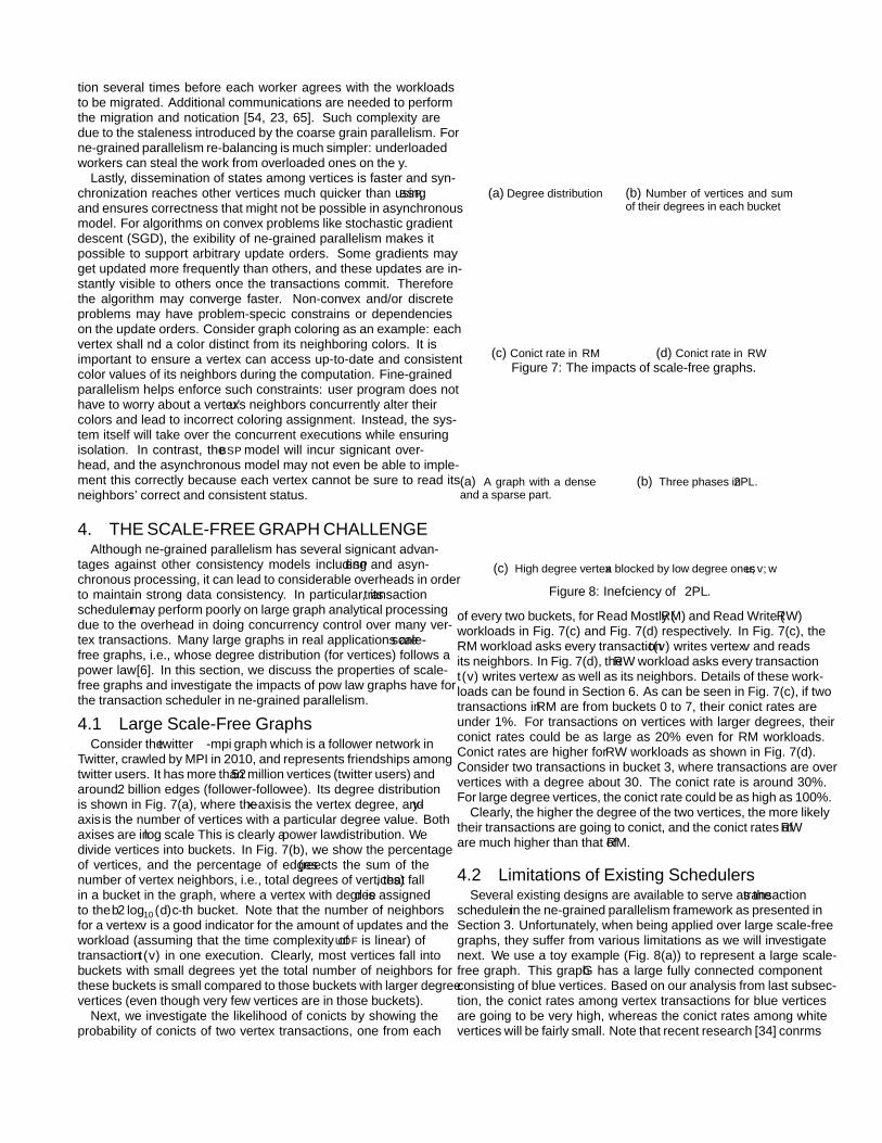
tages against other consistency models including BSP and asyn-chronous processing, it can lead to considerable overheads in orderto maintain strong data consistency. In particular, its transactionscheduler may perform poorly on large graph analytical processingdue to the overhead in doing concurrency control over many ver-tex transactions. Many large graphs in real applications are scale-free graphs, i.e., whose degree distribution (for vertices) follows apower law [6]. In this section, we discuss the properties of scale-free graphs and investigate the impacts of pow law graphs have forthe transaction scheduler in fine-grained parallelism.

4.1 Large Scale-Free GraphsConsider the twitter-mpi graph which is a follower network in

Twitter, crawled by MPI in 2010, and represents friendships amongtwitter users. It has more than 52 million vertices (twitter users) andaround 2 billion edges (follower-followee). Its degree distributionis shown in Fig. 7(a), where the x-axis is the vertex degree, and y-axis is the number of vertices with a particular degree value. Bothaxises are in log scale. This is clearly a power law distribution. Wedivide vertices into buckets. In Fig. 7(b), we show the percentageof vertices, and the percentage of edges (reflects the sum of thenumber of vertex neighbors, i.e., total degrees of vertices), that fallin a bucket in the graph, where a vertex with degree d is assignedto the b2 log10(d)c-th bucket. Note that the number of neighborsfor a vertex v is a good indicator for the amount of updates and theworkload (assuming that the time complexity of UDF is linear) oftransaction t(v) in one execution. Clearly, most vertices fall intobuckets with small degrees yet the total number of neighbors forthese buckets is small compared to those buckets with larger degreevertices (even though very few vertices are in those buckets).

Next, we investigate the likelihood of conflicts by showing theprobability of conflicts of two vertex transactions, one from each

101

103

105

107

100

101

102

103

104

105

count (in log)

degree (in log)

(a) Degree distribution

0

5

10

15

20

25

30

0 1 2 3 4 5 6 7 8 9 10111213

count (in %

)

bucket

# of vertices# of edges

(b) Number of vertices and sumof their degrees in each bucket

0 2 4 6 8 10 12bucket

0

2

4

6

8

10

12

bu

cke

t

0

0.1

0.2

0.3

0.4

0.5

(c) Conflict rate in RM

0 2 4 6 8 10 12bucket

0

2

4

6

8

10

12

bu

cke

t

0

0.2

0.4

0.6

0.8

1

(d) Conflict rate in RW

Figure 7: The impacts of scale-free graphs.

uvw

a

b

(a) A graph with a denseand a sparse part.

time

computing

shrinkinggrowing

locks

t(u)

(b) Three phases in 2PL.

time

locks

v awu

(c) High degree vertex a blocked by low degree ones u, v, w

Figure 8: Inefficiency of 2PL.

of every two buckets, for Read Mostly (RM) and Read Write (RW)workloads in Fig. 7(c) and Fig. 7(d) respectively. In Fig. 7(c), theRM workload asks every transaction t(v) writes vertex v and readsits neighbors. In Fig. 7(d), the RW workload asks every transactiont(v) writes vertex v as well as its neighbors. Details of these work-loads can be found in Section 6. As can be seen in Fig. 7(c), if twotransactions in RM are from buckets 0 to 7, their conflict rates areunder 1%. For transactions on vertices with larger degrees, theirconflict rates could be as large as 20% even for RM workloads.Conflict rates are higher for RW workloads as shown in Fig. 7(d).Consider two transactions in bucket 3, where transactions are oververtices with a degree about 30. The conflict rate is around 30%.For large degree vertices, the conflict rate could be as high as 100%.

Clearly, the higher the degree of the two vertices, the more likelytheir transactions are going to conflict, and the conflict rates of RWare much higher than that of RM.

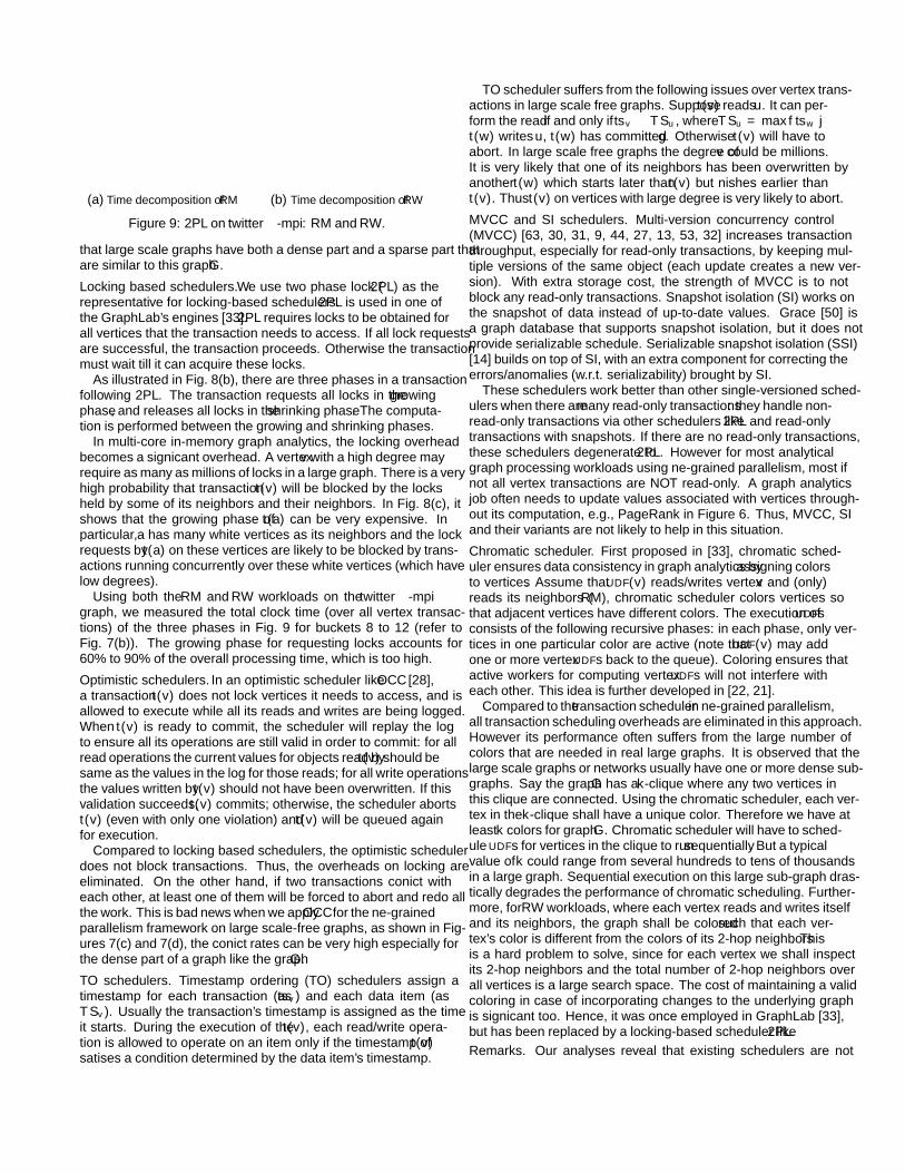
4.2 Limitations of Existing SchedulersSeveral existing designs are available to serve as the transaction

scheduler in the fine-grained parallelism framework as presented inSection 3. Unfortunately, when being applied over large scale-freegraphs, they suffer from various limitations as we will investigatenext. We use a toy example (Fig. 8(a)) to represent a large scale-free graph. This graph G has a large fully connected componentconsisting of blue vertices. Based on our analysis from last subsec-tion, the conflict rates among vertex transactions for blue verticesare going to be very high, whereas the conflict rates among whitevertices will be fairly small. Note that recent research [34] confirms

0%

20%

40%

60%

80%

100%

8 9 10 11 12

pe

rce

nta

ge

bucket

Grow Compute Shrink

(a) Time decomposition of RM

0%

20%

40%

60%

80%

100%

8 9 10 11 12

pe

rce

nta

ge

bucket

Grow Compute Shrink

(b) Time decomposition of RW

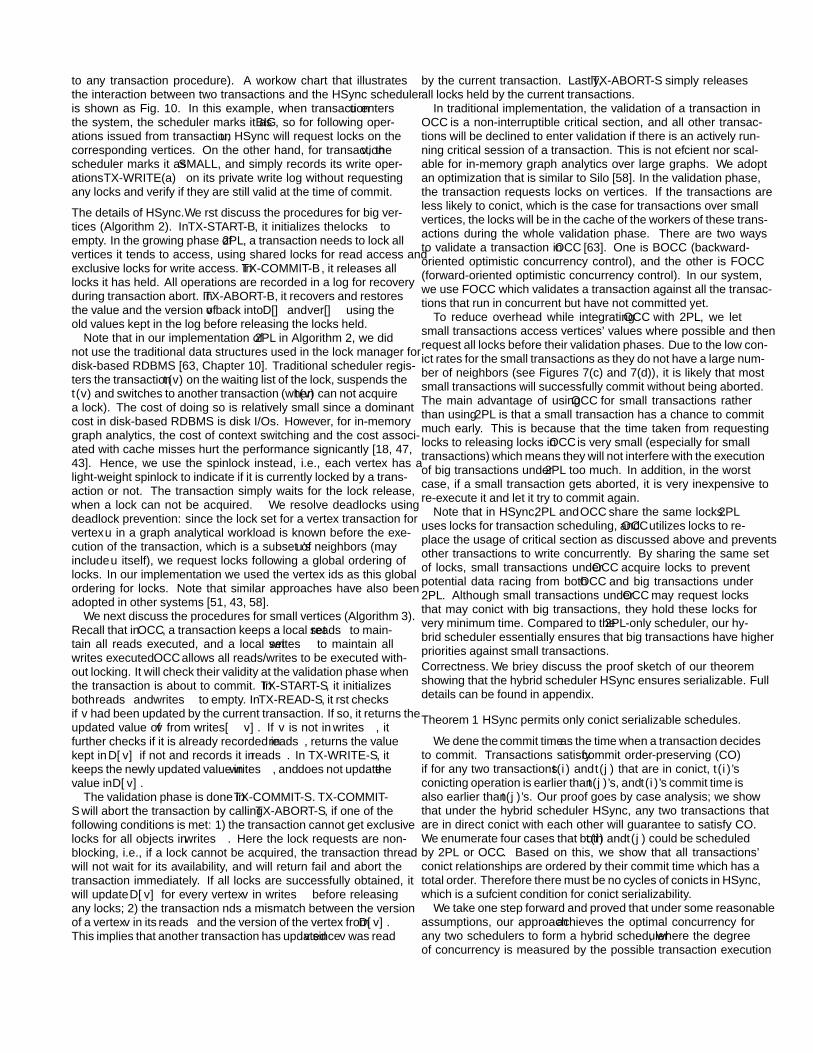
Figure 9: 2PL on twitter-mpi: RM and RW.

that large scale graphs have both a dense part and a sparse part thatare similar to this graph G.

Locking based schedulers. We use two phase lock (2PL) as therepresentative for locking-based schedulers. 2PL is used in one ofthe GraphLab’s engines [33]. 2PL requires locks to be obtained forall vertices that the transaction needs to access. If all lock requestsare successful, the transaction proceeds. Otherwise the transactionmust wait till it can acquire these locks.

As illustrated in Fig. 8(b), there are three phases in a transactionfollowing 2PL. The transaction requests all locks in the growingphase, and releases all locks in the shrinking phase. The computa-tion is performed between the growing and shrinking phases.

In multi-core in-memory graph analytics, the locking overheadbecomes a significant overhead. A vertex v with a high degree mayrequire as many as millions of locks in a large graph. There is a veryhigh probability that transaction t(v) will be blocked by the locksheld by some of its neighbors and their neighbors. In Fig. 8(c), itshows that the growing phase of t(a) can be very expensive. Inparticular, a has many white vertices as its neighbors and the lockrequests by t(a) on these vertices are likely to be blocked by trans-actions running concurrently over these white vertices (which havelow degrees).

Using both the RM and RW workloads on the twitter-mpigraph, we measured the total clock time (over all vertex transac-tions) of the three phases in Fig. 9 for buckets 8 to 12 (refer toFig. 7(b)). The growing phase for requesting locks accounts for60% to 90% of the overall processing time, which is too high.

Optimistic schedulers. In an optimistic scheduler like OCC [28],a transaction t(v) does not lock vertices it needs to access, and isallowed to execute while all its reads and writes are being logged.When t(v) is ready to commit, the scheduler will replay the logto ensure all its operations are still valid in order to commit: for allread operations the current values for objects read by t(v) should besame as the values in the log for those reads; for all write operationsthe values written by t(v) should not have been overwritten. If thisvalidation succeeds, t(v) commits; otherwise, the scheduler abortst(v) (even with only one violation) and t(v) will be queued againfor execution.

Compared to locking based schedulers, the optimistic schedulerdoes not block transactions. Thus, the overheads on locking areeliminated. On the other hand, if two transactions conflict witheach other, at least one of them will be forced to abort and redo allthe work. This is bad news when we apply OCC for the fine-grainedparallelism framework on large scale-free graphs, as shown in Fig-ures 7(c) and 7(d), the conflict rates can be very high especially forthe dense part of a graph like the graph G.

TO schedulers. Timestamp ordering (TO) schedulers assign atimestamp for each transaction (as tsv) and each data item (asTSv). Usually the transaction’s timestamp is assigned as the timeit starts. During the execution of the t(v), each read/write opera-tion is allowed to operate on an item only if the timestamp of t(v)satisfies a condition determined by the data item’s timestamp.

TO scheduler suffers from the following issues over vertex trans-actions in large scale free graphs. Suppose t(v) reads u. It can per-form the read if and only if tsv ≥ TSu, where TSu = max{tsw |t(w) writes u, t(w) has committed}. Otherwise t(v) will have toabort. In large scale free graphs the degree of v could be millions.It is very likely that one of its neighbors has been overwritten byanother t(w) which starts later than t(v) but finishes earlier thant(v). Thus t(v) on vertices with large degree is very likely to abort.

MVCC and SI schedulers. Multi-version concurrency control(MVCC) [63, 30, 31, 9, 44, 27, 13, 53, 32] increases transactionthroughput, especially for read-only transactions, by keeping mul-tiple versions of the same object (each update creates a new ver-sion). With extra storage cost, the strength of MVCC is to notblock any read-only transactions. Snapshot isolation (SI) works onthe snapshot of data instead of up-to-date values. Grace [50] isa graph database that supports snapshot isolation, but it does notprovide serializable schedule. Serializable snapshot isolation (SSI)[14] builds on top of SI, with an extra component for correcting theerrors/anomalies (w.r.t. serializability) brought by SI.

These schedulers work better than other single-versioned sched-ulers when there are many read-only transactions: they handle non-read-only transactions via other schedulers like 2PL and read-onlytransactions with snapshots. If there are no read-only transactions,these schedulers degenerate to 2PL. However for most analyticalgraph processing workloads using fine-grained parallelism, most ifnot all vertex transactions are NOT read-only. A graph analyticsjob often needs to update values associated with vertices through-out its computation, e.g., PageRank in Figure 6. Thus, MVCC, SIand their variants are not likely to help in this situation.

Chromatic scheduler. First proposed in [33], chromatic sched-uler ensures data consistency in graph analytics by assigning colorsto vertices. Assume that UDF(v) reads/writes vertex v and (only)reads its neighbors (RM), chromatic scheduler colors vertices sothat adjacent vertices have different colors. The execution of UDFsconsists of the following recursive phases: in each phase, only ver-tices in one particular color are active (note that UDF(v) may addone or more vertex UDFs back to the queue). Coloring ensures thatactive workers for computing vertex UDFs will not interfere witheach other. This idea is further developed in [22, 21].

Compared to the transaction scheduler in fine-grained parallelism,all transaction scheduling overheads are eliminated in this approach.However its performance often suffers from the large number ofcolors that are needed in real large graphs. It is observed that thelarge scale graphs or networks usually have one or more dense sub-graphs. Say the graph G has a k-clique where any two vertices inthis clique are connected. Using the chromatic scheduler, each ver-tex in the k-clique shall have a unique color. Therefore we have atleast k colors for graphG. Chromatic scheduler will have to sched-ule UDFs for vertices in the clique to run sequentially. But a typicalvalue of k could range from several hundreds to tens of thousandsin a large graph. Sequential execution on this large sub-graph dras-tically degrades the performance of chromatic scheduling. Further-more, for RW workloads, where each vertex reads and writes itselfand its neighbors, the graph shall be colored such that each ver-tex’s color is different from the colors of its 2-hop neighbors. Thisis a hard problem to solve, since for each vertex we shall inspectits 2-hop neighbors and the total number of 2-hop neighbors overall vertices is a large search space. The cost of maintaining a validcoloring in case of incorporating changes to the underlying graphis significant too. Hence, it was once employed in GraphLab [33],but has been replaced by a locking-based scheduler like 2PL.Remarks. Our analyses reveal that existing schedulers are not

Algorithm 1 TX-START (v)Require: vertices values in D[] . Graph dataRequire: vertices version in ver[] . Meta-data for schedulingRequire: vertices locks in L[] . Fine-grained locks

1: if d(v) ≥ threshold τ then2: BIG← true; TX-START-B (v);3: else4: BIG← false; TX-START-S (v);5: set version = concatenation of ThreadID and counter;6: counter++;

schedulertransaction u transaction vTX-SRART(u) TX-START(v)

TX-WRITE(a)

TX-READ(a)

TX-WRITE(w)

mark as BIG

lock a

lock w

mark as SMALL

record a

TX-COMMIT

validate

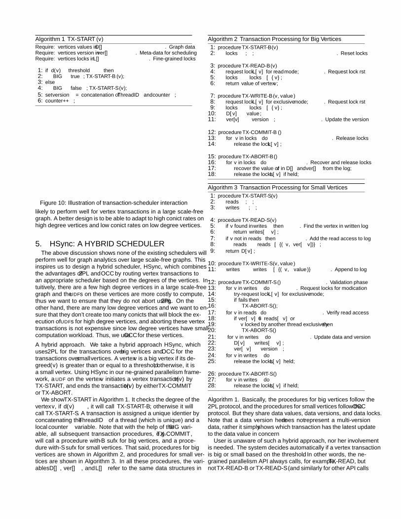
Figure 10: Illustration of transaction-scheduler interactionlikely to perform well for vertex transactions in a large scale-freegraph. A better design is to be able to adapt to high conflict rates onhigh degree vertices and low conflict rates on low degree vertices.

5. HSync: A HYBRID SCHEDULERThe above discussion shows none of the existing schedulers will

perform well for graph analytics over large scale-free graphs. Thisinspires us to design a hybrid scheduler, HSync, which combinesthe advantages of 2PL and OCC by routing vertex transactions toan appropriate scheduler based on the degrees of the vertices. In-tuitively, there are a few high degree vertices in a large scale-freegraph and the UDFs on these vertices are more costly to compute,thus we want to ensure that they do not abort using 2PL. On theother hand, there are many low degree vertices and we want to en-sure that they don’t create too many conflicts that will block the ex-ecution of UDFs for high degree vertices, and aborting these vertextransactions is not expensive since low degree vertices have smallcomputation workload. Thus, we use OCC for these vertices.

A hybrid approach. We take a hybrid approach HSync, whichuses 2PL for the transactions over big vertices and OCC for thetransactions over small vertices. A vertex v is a big vertex if its de-gree d(v) is greater than or equal to a threshold τ ; otherwise, it isa small vertex. Using HSync in our fine-grained parallelism frame-work, a UDF on the vertex v initiates a vertex transaction t(v) byTX-START, and ends the transaction t(v) by either TX-COMMITor TX-ABORT.

We show TX-START in Algorithm 1. It checks the degree of thevertex v, if d(v) ≥ τ , it will call TX-START-B; otherwise it willcall TX-START-S. A transaction is assigned a unique identifier byconcatenating the ThreadID of a thread (which is unique) and alocal counter variable. Note that with the help of the BIG vari-able, all subsequent transaction procedures, e.g. TX-COMMIT,will call a procedure with -B suffix for big vertices, and a proce-dure with -S suffix for small vertices. That said, procedures for bigvertices are shown in Algorithm 2, and procedures for small ver-tices are shown in Algorithm 3. In all these procedures, the vari-ables D[], ver[], and L[] refer to the same data structures in

Algorithm 2 Transaction Processing for Big Vertices1: procedure TX-START-B (v)2: locks← ∅; . Reset locks

3: procedure TX-READ-B (v)4: request lock L[v] for read mode; . Request lock first5: locks← locks ∪ {v};6: return value of vertex v;

7: procedure TX-WRITE-B (v, value)8: request lock L[v] for exclusive mode; . Request lock first9: locks← locks ∪ {v};

10: D[v]← value;11: ver[v]← version; . Update the version

12: procedure TX-COMMIT-B ()13: for v in locks do . Release locks14: release the lock L[v];

15: procedure TX-ABORT-B ()16: for v in locks do . Recover and release locks17: recover the value of v in D[] and ver[] from the log;18: release the locks L[v] if held;

Algorithm 3 Transaction Processing for Small Vertices1: procedure TX-START-S (v)2: reads← ∅;3: writes← ∅;

4: procedure TX-READ-S (v)5: if v found in writes then . Find the vertex in written log6: return writes[v];7: if v not in reads then . Add the read access to log8: reads← reads ∪ {(v, ver[v])};9: return D[v];

10: procedure TX-WRITE-S (v, value)11: writes← writes ∪ {(v, value)} . Append to log

12: procedure TX-COMMIT-S () . Validation phase13: for v in writes do . Request locks for modification14: try-request lock L[v] for exclusive mode;15: if fails then16: TX-ABORT-S ();17: for v in reads do . Verify read access18: if ver[v] 6= reads[v] or19: v locked by another thread exclusively then20: TX-ABORT-S ()21: for v in writes do . Update data and version22: D[v]← writes[v];23: ver[v]← version;24: for v in writes do25: release the locks L[v] held;

26: procedure TX-ABORT-S ()27: for v in writes do28: release the locks L[v] if held;

Algorithm 1. Basically, the procedures for big vertices follow the2PL protocol, and the procedures for small vertices follow the OCCprotocol. But they share data values, data versions, and data locks.Note that a data version here does not represent a multi-versiondata, rather it simply shows which transaction has the latest updateto the data value in concern.

User is unaware of such a hybrid approach, nor her involvementis needed. The system decides automatically if a vertex transactionis big or small based on the threshold τ . In other words, the fine-grained parallelism API always calls, for example, TX-READ, butnot TX-READ-B or TX-READ-S (and similarly for other API calls

to any transaction procedure). A workflow chart that illustratesthe interaction between two transactions and the HSync scheduleris shown as Fig. 10. In this example, when transaction u entersthe system, the scheduler marks it as BIG, so for following oper-ations issued from transaction u, HSync will request locks on thecorresponding vertices. On the other hand, for transaction v, thescheduler marks it as SMALL, and simply records its write oper-ations TX-WRITE(a) on its private write log without requestingany locks and verify if they are still valid at the time of commit.

The details of HSync. We first discuss the procedures for big ver-tices (Algorithm 2). In TX-START-B, it initializes the locks toempty. In the growing phase of 2PL, a transaction needs to lock allvertices it tends to access, using shared locks for read access andexclusive locks for write access. In TX-COMMIT-B, it releases alllocks it has held. All operations are recorded in a log for recoveryduring transaction abort. In TX-ABORT-B, it recovers and restoresthe value and the version of v back into D[] and ver[] using theold values kept in the log before releasing the locks held.

Note that in our implementation of 2PL in Algorithm 2, we didnot use the traditional data structures used in the lock manager fordisk-based RDBMS [63, Chapter 10]. Traditional scheduler regis-ters the transaction t(v) on the waiting list of the lock, suspends thet(v) and switches to another transaction (when t(v) can not acquirea lock). The cost of doing so is relatively small since a dominantcost in disk-based RDBMS is disk I/Os. However, for in-memorygraph analytics, the cost of context switching and the cost associ-ated with cache misses hurt the performance significantly [18, 47,43]. Hence, we use the spinlock instead, i.e., each vertex has alight-weight spinlock to indicate if it is currently locked by a trans-action or not. The transaction simply waits for the lock release,when a lock can not be acquired. We resolve deadlocks usingdeadlock prevention: since the lock set for a vertex transaction forvertex u in a graph analytical workload is known before the exe-cution of the transaction, which is a subset of u’s neighbors (mayinclude u itself), we request locks following a global ordering oflocks. In our implementation we used the vertex ids as this globalordering for locks. Note that similar approaches have also beenadopted in other systems [51, 43, 58].

We next discuss the procedures for small vertices (Algorithm 3).Recall that in OCC, a transaction keeps a local set reads to main-tain all reads executed, and a local set writes to maintain allwrites executed. OCC allows all reads/writes to be executed with-out locking. It will check their validity at the validation phase whenthe transaction is about to commit. In TX-START-S, it initializesboth reads and writes to empty. In TX-READ-S, it first checksif v had been updated by the current transaction. If so, it returns theupdated value of v from writes[v]. If v is not in writes, itfurther checks if it is already recorded in reads, returns the valuekept in D[v] if not and records it in reads. In TX-WRITE-S, itkeeps the newly updated value in writes, and does not update thevalue in D[v].

The validation phase is done in TX-COMMIT-S. TX-COMMIT-S will abort the transaction by calling TX-ABORT-S, if one of thefollowing conditions is met: 1) the transaction cannot get exclusivelocks for all objects in writes. Here the lock requests are non-blocking, i.e., if a lock cannot be acquired, the transaction threadwill not wait for its availability, and will return fail and abort thetransaction immediately. If all locks are successfully obtained, itwill update D[v] for every vertex v in writes before releasingany locks; 2) the transaction finds a mismatch between the versionof a vertex v in its reads and the version of the vertex from D[v].This implies that another transaction has updated v since v was read

by the current transaction. Lastly, TX-ABORT-S simply releasesall locks held by the current transactions.

In traditional implementation, the validation of a transaction inOCC is a non-interruptible critical section, and all other transac-tions will be declined to enter validation if there is an actively run-ning critical session of a transaction. This is not efficient nor scal-able for in-memory graph analytics over large graphs. We adoptan optimization that is similar to Silo [58]. In the validation phase,the transaction requests locks on vertices. If the transactions areless likely to conflict, which is the case for transactions over smallvertices, the locks will be in the cache of the workers of these trans-actions during the whole validation phase. There are two waysto validate a transaction in OCC [63]. One is BOCC (backward-oriented optimistic concurrency control), and the other is FOCC(forward-oriented optimistic concurrency control). In our system,we use FOCC which validates a transaction against all the transac-tions that run in concurrent but have not committed yet.

To reduce overhead while integrating OCC with 2PL, we letsmall transactions access vertices’ values where possible and thenrequest all locks before their validation phases. Due to the low con-flict rates for the small transactions as they do not have a large num-ber of neighbors (see Figures 7(c) and 7(d)), it is likely that mostsmall transactions will successfully commit without being aborted.The main advantage of using OCC for small transactions ratherthan using 2PL is that a small transaction has a chance to commitmuch early. This is because that the time taken from requestinglocks to releasing locks in OCC is very small (especially for smalltransactions) which means they will not interfere with the executionof big transactions under 2PL too much. In addition, in the worstcase, if a small transaction gets aborted, it is very inexpensive tore-execute it and let it try to commit again.

Note that in HSync, 2PL and OCC share the same locks. 2PLuses locks for transaction scheduling, and OCC utilizes locks to re-place the usage of critical section as discussed above and preventsother transactions to write concurrently. By sharing the same setof locks, small transactions under OCC acquire locks to preventpotential data racing from both OCC and big transactions under2PL. Although small transactions under OCC may request locksthat may conflict with big transactions, they hold these locks forvery minimum time. Compared to the 2PL-only scheduler, our hy-brid scheduler essentially ensures that big transactions have higherpriorities against small transactions.Correctness. We briefly discuss the proof sketch of our theoremshowing that the hybrid scheduler HSync ensures serializable. Fulldetails can be found in appendix.

Theorem 1 HSync permits only conflict serializable schedules.

We define the commit time as the time when a transaction decidesto commit. Transactions satisfy commit order-preserving (CO)if for any two transactions t(i) and t(j) that are in conflict, t(i)’sconflicting operation is earlier than t(j)’s, and t(i)’s commit time isalso earlier than t(j)’s. Our proof goes by case analysis; we showthat under the hybrid scheduler HSync, any two transactions thatare in direct conflict with each other will guarantee to satisfy CO.We enumerate four cases that both t(i) and t(j) could be scheduledby 2PL or OCC. Based on this, we show that all transactions’conflict relationships are ordered by their commit time which has atotal order. Therefore there must be no cycles of conflicts in HSync,which is a sufficient condition for conflict serializability. �

We take one step forward and proved that under some reasonableassumptions, our approach achieves the optimal concurrency forany two schedulers to form a hybrid scheduler, where the degreeof concurrency is measured by the possible transaction execution

t(u) u . . . . . . 3(a) 2PL t(v) v a 3

t(w) u w a 3

t(u) u w a b . . . 7(b) OCC t(v) v a 3

t(w) u w a 3

t(u) u w a b . . . 3(c) HSync t(v) v a 3

t(w) u w a 7time−−−−−−−−−−−−−−−−−−−−−−−−−−−−−−−→

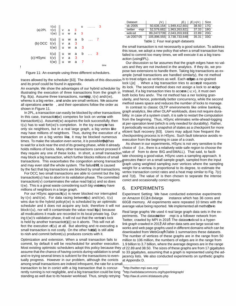
Figure 11: An example using three different schedulers.

traces allowed by the scheduler [63]. The details of this discussionand its proof could be found in appendix.An example. We show the advantages of our hybrid scheduler byillustrating the execution of three transactions from the graph inFig. 8(a). Assume three transactions, namely t(u), t(v) and t(w),where u is a big vertex , and v andw are small vertices. We assumeall operations are write, and their operations follow the order asshown in Figure 11.

In 2PL, a transaction can easily be blocked by other transactions.In this case, transaction t(w) competes for lock on vertex u withtransaction t(u). Assume t(w) acquires the lock successfully, thent(u) has to wait for t(w)’s completion. In the toy example u hasonly six neighbors, but in a real large graph, a big vertex like umay have millions of neighbors. Thus, during the execution of atransaction on a big vertex like u, it may be blocked numeroustimes. To make the situation even worse, it is possible that t(u) hasto wait for a lock near the end of its growing phase, while it alreadyholds millions of locks. Many other transactions cannot proceed ifthey require any one of these locks. In short, a small transactionmay block a big transaction, which further blocks millions of smalltransactions. This exacerbates the congestion among transactionsand may even stall the whole system. The failure of 2PL is causedby the fact that big transactions are blocked by small transactions.

For OCC, two small transactions are able to commit but the bigtransaction t(u) has to abort in its validation phase. The committedtransaction t(v) “contaminates” the value read by t(u) and so doest(w). This is a great waste considering such big vertex u may havemillions of neighbors in a large graph.

For our HSync approach, t(u) is never blocked nor interruptedby t(v) and t(w). For data racing between t(u) and t(w), t(u)wins due to the hybrid policy: t(w) is scheduled by an optimisticscheduler and it does not acquire any lock; therefore it will notblock t(u), nor will it contaminate the value read by t(u) becauseall modifications it made are recorded in its local private log. Dur-ing t(w)’s validation phase, it will find out that the vertex a’s lockis held by another transaction (t(u)) so it aborts. This will not af-fect the execution of t(u) at all. But aborting and re-executing asmall transaction is not costly. On the other hand, t(v) is still ableto finish and commit before t(u) produces conflicts with it.

Optimization and extension. When a small transaction fails tocommit, by default it will be rescheduled for another execution.Most existing optimistic schedulers adopt this policy because theyassume that the chance of having conflicts during validation is smalland re-trying several times is sufficient for the transactions to even-tually progress. However in our problem, although the conflictsamong small transactions are indeed infrequent, the rate for a smalltransaction to be in conflict with a big transaction that is concur-rently running is not negligible, and a big transaction could be longstanding as well due to its heavier workload. Thus, simply retrying

Dataset |V | |E| |E|/|V | Sizesk-2005 50,636,154 1,949,412,601 38.50 17Gtwitter-mpi 52,579,682 1,963,263,821 37.33 18Gwdc-sd 89,2472739 2,043,203,933 22.89 20Guk-2007-05 105,896,555 3,738,733,648 35.31 33G

Table 1: Four real graph datasetsthe small transaction is not necessarily a good solution. To addressthis issue, we adopt a new policy that when a small transaction hasfailed to commit too many times, we will execute it as a big trans-action (using 2PL).

Our discussion so far assumes that the graph edges have no val-ues and they are not involved in the analytics. If they do, we pro-pose two extensions to handle them. Taking big transactions as ex-ample (small transactions are handled similarly), the first methodis to treat edges as vertices as well. Each edge e has a fine-grainedlock L[e]. When a big transaction tries to access e, it requestsits lock. The second method does not assign a lock to an edge e.Instead, if a big transaction tries to access e = (u, v), it must ownboth locks for u and v. The first method has a finer locking gran-ularity, and hence, potentially better concurrency, while the secondmethod saves space and reduces the number of locks to manage.

In contrast to classic OLTP environments like online banking,graph analytics, like other OLAP workloads, does not require dura-bility: in case of a system crash, it is safe to restart the computationfrom the beginning. Thus, HSync eliminates write-ahead-loggingat per-operation level (which is only needed for durability). Rather,it periodically records a snapshot of states as a checkpoint for moreefficient fault recovery [63]. Users may adjust how frequent thecheckpointing process is in HSync. Such fault tolerance avoids re-execution from the beginning in case of a crash.

As shown in our experiments, HSync is not very sensitive to thechoice of τ (i.e., there is a relatively wide safe region to choose thevalue of τ from to define BIG and SMALL). That said, to facili-tate choosing a good τ value, HSync uses a sampling approach. Itexecutes the UDF on a small sample graph, sampled from the inputgraph using weighted sampling over vertices where the samplingweight for a vertex u is proportional to its degree, to estimate thevertex transaction conflict rates and a heat map similar to Fig. 7(c)and 7(d). The value of τ is then chosen to separate the intenseconflict and occasionally conflict regions.

6. EXPERIMENTSExperiment Setting: We have conducted extensive experimentson Amazon EC2 c4.8xlarge instance which has 36 cores and60GB memory. All experiments were repeated 10 times with theaverage value being reported. We implemented all methods in C++.

Real large graphs: We used 4 real large graph data sets in the ex-periments. The dataset twitter-mpi is a follower network fromTwitter, crawled by MPI in 2010.2 The dataset wdc-sd is a hyper-link graph crawled in 2012.3 All other data sets are large social net-works and web page graphs used in different domains which can bedownloaded from WebGraph.4 Table 1 summarizes these datasets.The number of vertices of these graphs are in the range from 50million to 106 million, the numbers of edges are in the range from1.9 billion to 3.7 billion, where the average degrees are in the rangeof 22.89 and 38.50. The sizes of these graphs are from 17 gigabytesto 33 gigabytes, assuming that a graph is represented using the ad-jacency lists. We also conducted experiments on synthetic graphsat Appendix D.

2http://twitter.mpi-sws.org/3http://webdatacommons.org/hyperlinkgraph/4http://law.di.unimi.it/datasets.php

2PL OCC Chromatic TO MVTO 2V2PL HSync

0

2

4

6

8

10

1 4 8 16 24 32(a) wdc-sd @ RM

0

2

4

6

8

10

12

1 4 8 16 24 32(b) sk-2005 @ RM

0

2

4

6

1 4 8 16 24 32(c) twitter-mpi @ RM

0

2

4

6

8

10

12

1 4 8 16 24 32(d) uk-2007-05 @ RM

0

2

4

6

1 4 8 16 24 32(e) wdc-sd @ RW

0

2

4

6

1 4 8 16 24 32(f) sk-2005 @ RW

0

2

4

1 4 8 16 24 32(g) twitter-mpi @ RW

0

2

4

6

1 4 8 16 24 32(h) uk-2007-05 @ RW

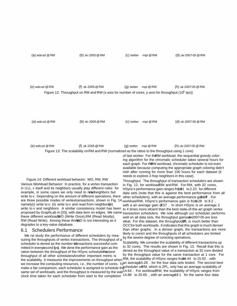
Figure 12: Throughput on RM and RW (x-axis for number of cores, y-axis for throughput (×106 tps))2PL OCC Chromatic TO MVTO 2V2PL HSync

0

4

8

12

1 4 8 16 24 32(a) wdc-sd @ RM

0

4

8

12

1 4 8 16 24 32(b) sk-2005 @ RM

0

4

8

12

16

1 4 8 16 24 32(c) twitter-mpi @ RM

0

4

8

12

1 4 8 16 24 32(d) uk-2007-05 @ RM

0

4

8

12

1 4 8 16 24 32(e) wdc-sd @ RW

048

1216

1 4 8 16 24 32(f) sk-2005 @ RW

048

121620

1 4 8 16 24 32(g) twitter-mpi @ RW

048

1216

1 4 8 16 24 32(h) uk-2007-05 @ RW

Figure 13: The scalability on RM and RW (normalized as the ratios to the throughput using 1 core)

Write

Read

Write

Write

Figure 14: Different workload behavior: WO, RM, RWVarious Workload Behavior: In practice, for a vertex transactionin t(v), v itself and its neighbors usually play different roles: forexample, in some cases we only need to read v’s neighbors butwrite to v. Depending on the amount of different operations, thereare three possible modes of vertextransactions, shown in Fig. 14,namely (i) write to v; (ii) write to v and read from neighbors; (iii)write to v and neighbors. A similar consistency model has beenproposed by GraphLab in [33], with data item on edges. We namethese different workloads WO (Write Once), RM (Read Mostly),RW (Read Write). Among these three, WO is not interesting as itdegrades to a key-value database.

6.1 Schedulers PerformanceWe first study the performance of different schedulers by mea-

suring the throughputs of vertex transactions. The throughput of ascheduler is defined as the number of transactions successful com-mitted in every second (tps). We define the performance gain as theration between the throughput of the HSync scheduler vs. the bestthroughput of all other schedulers. Another important metric isthe scalability. It measures the improvements on throughput whenwe increase the computing resources, i.e., the number of cores. Tomake a fair comparison, each scheduler is assigned to schedule thesame set of workloads, and the throughput is measured by the wallclock time taken for each scheduler from start to the completion

of last worker. For the RM workload, the sequential greedy color-ing algorithm for the chromatic scheduler takes several hours foreach graph. For the RW workload, chromatic scheduler is not evenavailable because computing the appropriate graph coloring didn’tfinish after running for more than 100 hours for each dataset (itneeds to explore 2-hop neighbors in this case).Throughput. The throughput of transaction schedulers are shownin Fig. 12, for workload RM and RW. For RM, with 32 cores,HSync’s performance gain ranges from 1.91 to 2.23 for differentdata sets (note that this is against the best performance from allother schedulers), with an average performance gain of 2.07. Forworkload RW, HSync’s performance gain is from 1.28 to 8.2,with a an average gain of 3.57. In short HSync is on average 2to 4 times more efficient than the best state-of-the-art graph vertextransaction schedulers. We note although our scheduler performswell on all data sets, the throughput gains on uk-2007-05 are lessideal. For this dataset, the throughput of 2PL is much better thanOCC for both workloads. It indicates that this graph is much denserthan other graphs. In a denser graph, the transactions are morelikely to conflict and the throughputs of all schedulers are limitedby the severe degree of conflicting operations.Scalability. We consider the scalability of different transactions upto 32 cores. The results are shown in Fig. 13. Recall that this isdefined as the throughput value of a transaction at 32 core dividedby the throughput value for the same transaction at 1 core. ForRM, the scalability of HSync ranges from 14.44 to 15.92, withan average 15.28, for the four data sets tested. The second bestscheduler on RM, which is 2PL, only has an average scalability of14.64. For workload RW, the scalability of HSync ranges from14.88 to 20.65, with an average 18.1 for the same four data

SMALL percentage Overall Throughput SMALL abort rate

0%

20%

40%

60%

80%

100%

10 102

103

104

105

0

2

4

6

8

10

(a) wdc-sd @ RM

0%

20%

40%

60%

80%

100%

10 102

103

104

105

0

2

4

6

8

10

12

(b) sk-2005 @ RM

0%

20%

40%

60%

80%

100%

10 102

103

104

105

0

2

4

6

(c) twitter-mpi @ RM

0%

20%

40%

60%

80%

100%

10 102

103

104

105

0

2

4

6

8

10

12

(d) uk-2007-05 @ RM

0%

20%

40%

60%

80%

100%

10 102

103

104

105

0

2

4

6

(e) wdc-sd @ RW

0%

20%

40%

60%

80%

100%

10 102

103

104

105

0

2

4

6

(f) sk-2005 @ RW

0%

20%

40%

60%

80%

100%

10 102

103

104

105

0

2

4

(g) twitter-mpi @ RW

0%

20%

40%

60%

80%

100%

10 102

103

104

105

0

2

4

6

(h) uk-2007-05 @ RW

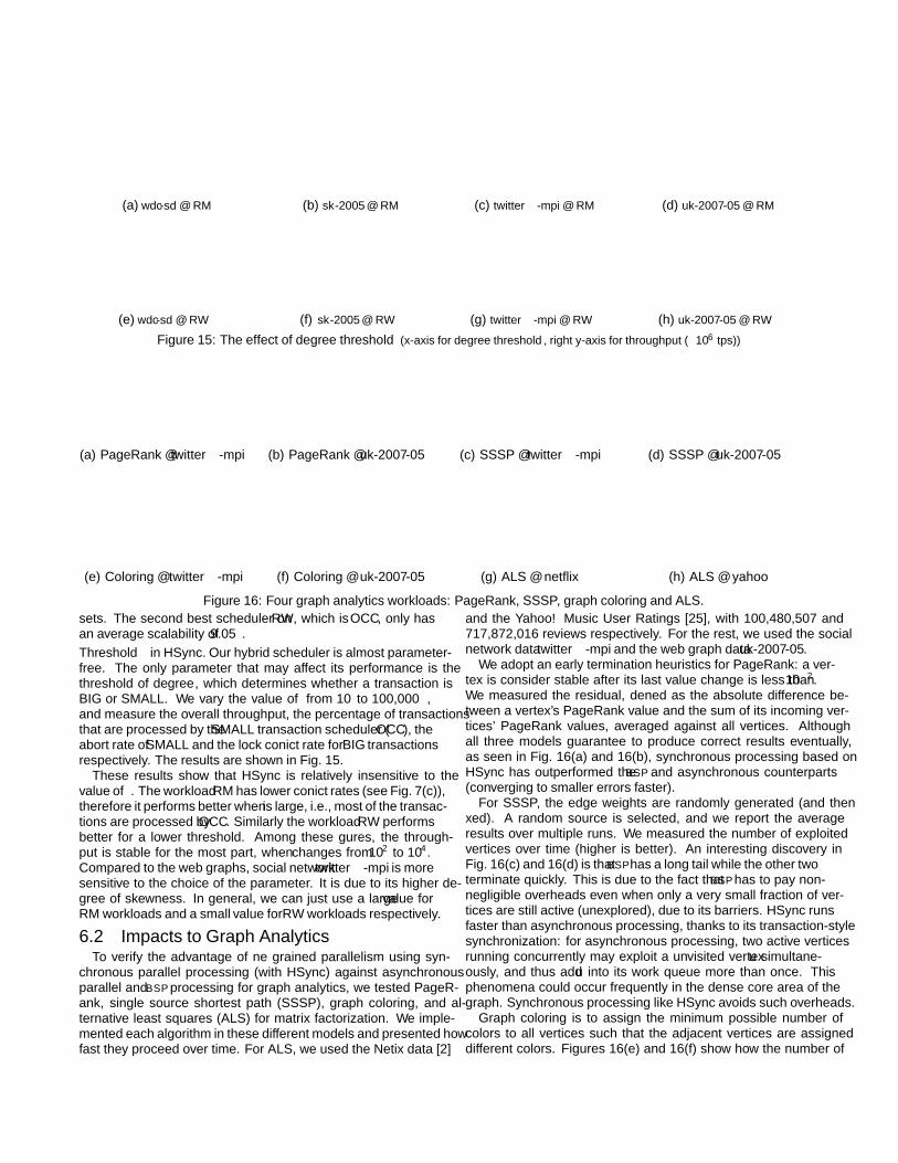
Figure 15: The effect of degree threshold τ (x-axis for degree threshold τ , right y-axis for throughput (×106 tps))

0.0

0.2

0.4

0.6

0.8

1.0

0 10 20 30 40 50 60

resid

ual

time (in second)

HSyncAsync

BSP

(a) PageRank @ twitter-mpi

0.0

0.2

0.4

0.6

0.8

1.0

0 5 10 15 20 25 30

resid

ual

time (in second)

HSyncAsync

BSP

(b) PageRank @ uk-2007-05

0

107

2*107

3*107

4*107

5*107

0 5 10 15 20 25 30 35 40explo

ited

time (in second)

HSyncAsync

BSP

(c) SSSP @ twitter-mpi

0

2*107

4*107

6*107

8*107

0 5 10 15 20 25 30 35 40

explo

ited

time (in second)

HSyncAsync

BSP

(d) SSSP @ uk-2007-05

0

100

200

300

400

0 50 100 150 200 250 300

cro

ss e

dges

time (in second)

HSyncAsync

BSP

(e) Coloring @ twitter-mpi

0

2*105

4*105

6*105

8*105

106

0 50 100 150 200 250

cro

ss e

dges

time (in second)

HSyncAsync

BSP

(f) Coloring @ uk-2007-05

1.0

1.5

2.0

2.5

0 20 40 60 80 100

rmse

time (in second)

HSyncAsync

BSP

(g) ALS @ netflix

1.0

1.5

2.0

2.5

0 100 200 300 400 500

rmse

time (in second)

HSyncAsync

BSP

(h) ALS @ yahoo

Figure 16: Four graph analytics workloads: PageRank, SSSP, graph coloring and ALS.sets. The second best scheduler on RW, which is OCC, only hasan average scalability of 9.05.Threshold τ in HSync. Our hybrid scheduler is almost parameter-free. The only parameter that may affect its performance is thethreshold of degree τ , which determines whether a transaction isBIG or SMALL. We vary the value of τ from 10 to 100,000,and measure the overall throughput, the percentage of transactionsthat are processed by the SMALL transaction scheduler (OCC), theabort rate of SMALL and the lock conflict rate for BIG transactionsrespectively. The results are shown in Fig. 15.

These results show that HSync is relatively insensitive to thevalue of τ . The workload RM has lower conflict rates (see Fig. 7(c)),therefore it performs better when τ is large, i.e., most of the transac-tions are processed by OCC. Similarly the workload RW performsbetter for a lower threshold. Among these figures, the through-put is stable for the most part, when τ changes from 102 to 104.Compared to the web graphs, social network twitter-mpi is moresensitive to the choice of the parameter. It is due to its higher de-gree of skewness. In general, we can just use a large τ value forRM workloads and a small τ value for RW workloads respectively.

6.2 Impacts to Graph AnalyticsTo verify the advantage of fine grained parallelism using syn-

chronous parallel processing (with HSync) against asynchronousparallel and BSP processing for graph analytics, we tested PageR-ank, single source shortest path (SSSP), graph coloring, and al-ternative least squares (ALS) for matrix factorization. We imple-mented each algorithm in these different models and presented howfast they proceed over time. For ALS, we used the Netflix data [2]

and the Yahoo! Music User Ratings [25], with 100,480,507 and717,872,016 reviews respectively. For the rest, we used the socialnetwork data twitter-mpi and the web graph data uk-2007-05.

We adopt an “early termination” heuristics for PageRank: a ver-tex is consider stable after its last value change is less than 10−2.We measured the residual, defined as the absolute difference be-tween a vertex’s PageRank value and the sum of its incoming ver-tices’ PageRank values, averaged against all vertices. Althoughall three models guarantee to produce correct results eventually,as seen in Fig. 16(a) and 16(b), synchronous processing based onHSync has outperformed the BSP and asynchronous counterparts(converging to smaller errors faster).

For SSSP, the edge weights are randomly generated (and thenfixed). A random source is selected, and we report the averageresults over multiple runs. We measured the number of exploitedvertices over time (higher is better). An interesting discovery inFig. 16(c) and 16(d) is that BSP has a “long tail” while the other twoterminate quickly. This is due to the fact that BSP has to pay non-negligible overheads even when only a very small fraction of ver-tices are still “active” (unexplored), due to its barriers. HSync runsfaster than asynchronous processing, thanks to its transaction-stylesynchronization: for asynchronous processing, two active verticesrunning concurrently may exploit a unvisited vertex u simultane-ously, and thus add u into its work queue more than once. Thisphenomena could occur frequently in the dense “core” area of thegraph. Synchronous processing like HSync avoids such overheads.

Graph coloring is to assign the minimum possible number ofcolors to all vertices such that the adjacent vertices are assigneddifferent colors. Figures 16(e) and 16(f) show how the number of

PR SSSP WCC Color ALSDataset T U T U T U T U N Y

PowerGraph 1268 381 58.8 90.2 197 210 m m 392 4956PowerLyra 662 m 37.5 m 107 m m m 164 1784GraphChi 3778 2424 701 2077 589 3090 848 820 >3000 >8000

HSync 181 42.7 48.8 66.7 30.1 31.9 174 59.8 74.6 901

Table 2: Efficiency of different systems. (End-to-end wall clocktime in seconds. T: twitter-mpi, U: uk-2007-05, N: netflix, Y:yahoo. m: memory limit exceeded.)

PR SSSP WCC Color ALSDataset T U T U T U T U N Y

PowerGraph 7.0 8.9 1.2 1.4 6.5 6.6 - - 5.3 5.5PowerLyra 3.7 - 0.8 - 3.6 - - - 2.2 2.0GraphChi 20.9 56.8 14.4 31.1 19.6 96.9 4.9 13.7 >40.2 >8.9

Table 3: Efficiency compared with HSync, running time as aratio to HSync’s running time. (T: twitter-mpi, U: uk-2007-05,N:netflix, Y: yahoo)

edges that have violated this rule (two neighbors still have the samecolor) decreases over time. Note the BSP in this case is too expen-sive to converge, and its results have been ignored in these figures.Clearly, the fine grained parallelism using HSync converges muchfaster than asynchronous processing; the latter has difficulty to con-verge on dataset uk-2007-05, possibly due to its smaller diameterand dense “core” (such that inconsistent readings and assignmentsin asynchronous processing are hard to converge).

ALS can be formalized as a bipartite graph. ALS works by fix-ing the values on the right side and updating the left side, thenvice visa. Note that there is no asynchronous parallel processingalgorithm that is able to guarantee correct results for ALS [33].That said, one can still execute a synchronous parallel processingalgorithm in an asynchronous manner, without requiring the cor-rectness of the final output, to understand its behavior. As seen inFig. 16(g) and 16(h), where they show how the root mean squareerror (RMSE) reduces over time, the asynchronous parallel pro-cessing approach could not converge at all, whereas both BSP andsynchronous parallel processing have shown much better perfor-mance. And fine-grained parallelism using synchronous parallelprocessing with HSync has clearly outperformed BSP.

6.3 System Performance ComparisonWe compared the performance of fine-grained parallelism us-

ing HSync against other graph analytics systems, including Pow-erGraph [15], PowerLyra [4], and GraphChi [24], using PageRank,SSSP, weakly connected component (WCC), graph coloring andALS. We conducted the PowerGraph and PowerLyra experimentswith a 16 node Amazon EC2 m3.2xlarge (8 cores, 30GB mem-ory) cluster, and GraphChi on a r3.8xlarge instance with 32cores, 244GB memory and 320GB SSD. The memory budget forGraphChi is set to 200GB which is much larger than the dataset.The (one-pass) data preparation time and I/O time are excluded.

We report the end-to-end wall clock running time of each ap-proach in Table 2, and each system’s running time as a ratio toHSync in Table 3. HSync outperforms other systems by 3x to100x folds in most cases. Note that PowerGraph and PowerLyraare cluster-based with 128 cores in total (from the cluster), andGraphchi and HSync run on a single node with 32 cores.

7. RELATED WORKMany existing graph systems including Neo4j [38], Trinity [55],

FlockDB [41], InfiniteGraph [40], Allegrograph [37], NetflixGraph[39], Titan [36] and HyperGraph-DB [19] support transactionalgraph processing at different levels. Trinity only provides the prim-itive functions for developers to lock and unlock vertices. DEXallows at most one read-write transaction, plus unlimited number

of concurrent read-only transactions. Neo4j and Titan use standardtwo-phase lock (2PL) to implement the vertex transaction sched-uler. The details of other systems are unknown due to lack of pub-lications and the fact that they are not open sourced.

There are also works in database systems where they assumestatic workloads (in particular, the types of transactions are knowna priori) and they rely on static analysis for improving transactionscheduler’s performance. For example, H-Store [56, 18, 20] pro-poses transaction processing systems based on the partition of datasuch that local transactions do not conflict and they can run con-currently without concurrency control. Calvin [57] is based on asimilar approach. These approaches rely on high quality partitionsof the data that lead to little or no cross-partition transactions. Af-ter that each worker is responsible for processing the transactions inone partition. Thus, they need strong knowledge about the transac-tions to execute a priori. These approaches work well on businessor e-commerce workloads like TPC-C and YCSB since the datacan be easily partitioned. However large scale graphs tend to forma “hyper-ball” [61] and are much hard to partition [29] while en-suring little or no cross-partition vertex transactions.

Mixing concurrency control schemes have been explored beforein the context of transaction processing in RDBMS [28, 49, 26]where schedulers that combine two or more CC schemes were de-signed. For example in real-time systems, 2PL is used for the trans-actions that must be answered in a timely manner, otherwise thesystem uses OCC [26]. However all these approaches employ se-rializable graph testing to ensure the correct interaction betweenmultiple (e.g., 2PL and OCC) schedulers. This hurts scalabilityand throughput since testing serializable graph is very expensive.Our approach does not require additional mechanism to maintainthe correctness between two different transaction schedulers.

Lastly, note that we have already reviewed the most closely re-lated work on different schedulers and parallel processing modelsfor graph analytics in Sections 2 and 4.2.

8. CONCLUSION AND FUTURE WORKWe introduce a new design for fine grained parallelism using

synchronous parallel processing for graph analytics. By exploringthe particular properties in large scale free graphs, we designed andimplemented the HSync scheduler that shows excellent through-put and scalability for processing vertex transactions. HSync inte-grates 2PL with OCC, and uses 2PL to schedule vertex transactionsfrom high degree vertices to avoid aborting them, and uses OCC toschedule vertex transactions from low degree vertices to reduce theoverall overheads they may introduce to the system. A careful anal-ysis and design show that the interaction between the two types ofschedulers in HSync lead to correct results. Experimental evalua-tion confirms the advantage of HSync over other approaches.

As for future work, it is interesting to explore how to utilize thenew hardware, specially hardware transactional memory (HTM),non-volatile random-access memory (NVRAM) and remote directmemory access (RDMA) for even better parallelism. Our focushere is in-memory multi-core architecture on a single node, but it ispossible to extend our hybrid scheduler to a distributed in-memorycluster [11, 60] with distributed transaction processing [12, 62, 5]on top of fast network infrastructures like InfiniBand and RoCE(RDMA). In principle, distributed schedulers, like distributed 2PLand distributed OCC can be combined together in a similar fash-ion to derive a distributed version of HSync. Nevertheless, thereare still significant research challenges as how to combine two dis-tributed schedulers safely to satisfy our aforementioned necessaryand sufficient condition to achieve conflict serializability, i.e., sat-isfying commit order-preserving.

AcknowledgmentsThe authors thank the helpful comments from the anonymous re-viewers. The work was supported by grant of Research GrantsCouncil of the Hong Kong SAR, China No. 14209314, The Chi-nese University of Hong Kong Direct Grant No. 4055048. Feifei Liwas supported in part by NSF grants 1251019 and 1302663. FeifeiLi was also supported in part by NSFC grant 61428204. We alsothank the generous gift from AWS Cloud Credits for Research fromAmazon.

9. REFERENCES[1] R. Angles and C. Gutierrez. Survey of graph database models. ACM

Comput. Surv., 40(1):1:1–1:39, Feb. 2008.[2] J. Bennett, S. Lanning, and Netflix. The Netflix prize. KDD Cup and

Workshop, 2007.[3] P. A. Bernstein, V. Hadzilacos, and N. Goodman. Concurrency

Control and Recovery in Database Systems. Addison-Wesley, 1987.[4] R. Chen, J. Shi, Y. Chen, and H. Chen. Powerlyra: Differentiated

graph computation and partitioning on skewed graphs. EuroSys ’15,pp. 1:1–1:15, 2015.

[5] Y. Chen, X. Wei, J. Shi, R. Chen, and H. Chen. Fast and generaldistributed transactions using rdma and htm. EuroSys ’16, page toappear, 2016.

[6] A. Clauset, C. R. Shalizi, and M. E. J. Newman. Power-lawdistributions in empirical data. SIAM Rev., 51(4):661–703, Nov.2009.

[7] T. David, R. Guerraoui, and V. Trigonakis. Everything you alwayswanted to know about synchronization but were afraid to ask. SOSP’13, pp. 33–48, 2013.

[8] J. Dean and S. Ghemawat. Mapreduce: Simplified data processing onlarge clusters. Commun. ACM, 51(1):107–113, Jan. 2008.

[9] C. Diaconu, C. Freedman, E. Ismert, P.-A. Larson, P. Mittal,R. Stonecipher, N. Verma, and M. Zwilling. Hekaton: Sql server’smemory-optimized oltp engine. SIGMOD ’13, pp. 1243–1254, 2013.

[10] S. N. Dorogovtsev, J. F. F. Mendes, and A. N. Samukhin. Structure ofgrowing networks with preferential linking. Phys. Rev. Lett.,85:4633–4636, Nov 2000.

[11] A. Dragojevic, D. Narayanan, M. Castro, and O. Hodson. Farm: Fastremote memory. NSDI ’14, pp. 401–414, Apr. 2014.

[12] A. Dragojevic, D. Narayanan, E. B. Nightingale, M. Renzelmann,A. Shamis, A. Badam, and M. Castro. No compromises: Distributedtransactions with consistency, availability, and performance. SOSP’15, pp. 54–70, 2015.

[13] J. M. Faleiro and D. J. Abadi. Rethinking serializable multiversionconcurrency control. Proc. VLDB Endow., 8(11):1190–1201, July2015.

[14] A. Fekete, D. Liarokapis, E. O’Neil, P. O’Neil, and D. Shasha.Making snapshot isolation serializable. ACM Trans. Database Syst.,30(2):492–528, June 2005.

[15] J. E. Gonzalez, Y. Low, H. Gu, D. Bickson, and C. Guestrin.Powergraph: Distributed graph-parallel computation on naturalgraphs. OSDI ’12, pp. 17–30, 2012.

[16] J. Gray and A. Reuter. Transaction Processing: Concepts andTechniques. Morgan Kaufmann Publishers Inc., 1st edition, 1992.

[17] M. Grund, P. Cudré-Mauroux, J. Krueger, and H. Plattner. Hybridgraph and relational query processing in main memory. DESWEB’13, pp. 23–24, April 2013.

[18] S. Harizopoulos, D. J. Abadi, S. Madden, and M. Stonebraker. OLTPthrough the looking glass, and what we found there. SIGMOD ’08,pp. 981–992, 2008.

[19] B. Iordanov. HyperGraphDB: a generalized graph database. WAIM’10, 2010.

[20] E. P. Jones, D. J. Abadi, and S. Madden. Low overhead concurrencycontrol for partitioned main memory databases. SIGMOD ’10, pp.603–614, 2010.

[21] T. Kaler. Chromatic scheduling of dynamic data-graph computations.Master’s thesis, Massachusetts Institute of Technology, 2013.

[22] T. Kaler, W. Hasenplaugh, T. B. Schardl, and C. E. Leiserson.Executing dynamic data-graph computations deterministically usingchromatic scheduling. SPAA ’14, 2014.

[23] Z. Khayyat, K. Awara, A. Alonazi, H. Jamjoom, D. Williams, andP. Kalnis. Mizan: A system for dynamic load balancing in large-scalegraph processing. EuroSys ’13, pp. 169–182, 2013.

[24] A. Kyrola, G. Blelloch, and C. Guestrin. Graphchi: Large-scalegraph computation on just a pc. OSDI ’12, pp. 31–46, 2012.

[25] Y. Labs.http://webscope.sandbox.yahoo.com/catalog.php?datatype=r.[Online; accessed 6-Mar-2016].

[26] K.-Y. Lam, T.-W. Kuo, B. Kao, T. S. Lee, and R. Cheng. Evaluationof concurrency control strategies for mixed soft real-time databasesystems. Information Systems, 27:149, 2002.

[27] P.-A. Larson, S. Blanas, C. Diaconu, C. Freedman, J. M. Patel, andM. Zwilling. High-performance concurrency control mechanisms formain-memory databases. Proc. VLDB Endow., 5(4):298–309, Dec.2011.

[28] G. Lausen. Concurrency control in database systems: A step towardsthe integration of optimistic methods and locking. ACM ’82, pp.64–68, 1982.

[29] J. Leskovec, K. J. Lang, A. Dasgupta, and M. W. Mahoney.Community structure in large networks: Natural cluster sizes and theabsence of large well-defined clusters. Internet Mathematics,6(1):29–123, 2009.

[30] J. Levandoski, D. Lomet, S. Sengupta, R. Stutsman, and R. Wang.High performance transactions in deuteronomy. CIDR ’15, January2015.

[31] J. Levandoski, D. Lomet, S. Sengupta, R. Stutsman, and R. Wang.Multi-version range concurrency control in deuteronomy. Proc.VLDB Endow., 8(13):2146–2157, Sept. 2015.

[32] D. B. Lomet, A. Fekete, R. Wang, and P. Ward. Multi-versionconcurrency via timestamp range conflict management. ICDE ’12,pp. 714–725, 2012.

[33] Y. Low, D. Bickson, J. Gonzalez, C. Guestrin, A. Kyrola, and J. M.Hellerstein. Distributed graphlab: A framework for machine learningand data mining in the cloud. Proc. VLDB Endow., 5(8):716–727,Apr. 2012.

[34] T. Maehara, T. Akiba, Y. Iwata, and K. Kawarabayashi. Computingpersonalized pagerank quickly by exploiting graph structures.PVLDB, 7(12):1023–1034, 2014.

[35] G. Malewicz, M. H. Austern, A. J. Bik, J. C. Dehnert, I. Horn,N. Leiser, and G. Czajkowski. Pregel: A system for large-scale graphprocessing. SIGMOD ’10, pp. 135–146, 2010.

[36] Aurelius Inc. http://thinkaurelius.github.io/titan/.[37] Franz Inc. http://www.franz.com/agraph/allegrograph/.[38] Neo Technology, Inc. . http://www.neo4j.org/.[39] Netflix Inc. https://github.com/Netflix/netflix-graph.[40] Objectivity Inc. http://www.objectivity.com/infinitegraph.[41] Twitter Inc. https://github.com/twitter/flockdb.[42] B. Mcmahan and M. Streeter. Delay-tolerant algorithms for

asynchronous distributed online learning. In Z. Ghahramani,M. Welling, C. Cortes, N. Lawrence, and K. Weinberger, editors,NIPS ’14, pp. 2915–2923, 2014.

[43] N. Narula, C. Cutler, E. Kohler, and R. Morris. Phase reconciliationfor contended in-memory transactions. OSDI ’14, pp. 511–524, 2014.

[44] T. Neumann, T. Mühlbauer, and A. Kemper. Fast serializablemulti-version concurrency control for main-memory databasesystems. SIGMOD ’15, pp. 677–689, 2015.

[45] D. Nguyen, A. Lenharth, and K. Pingali. A lightweight infrastructurefor graph analytics. SOSP ’13, pp. 456–471, 2013.

[46] J. Ousterhout, P. Agrawal, D. Erickson, C. Kozyrakis, J. Leverich,D. Mazières, S. Mitra, A. Narayanan, G. Parulkar, M. Rosenblum,S. M. Rumble, E. Stratmann, and R. Stutsman. The case forRAMClouds: Scalable high-performance storage entirely in dram.SIGOPS Oper. Syst. Rev., 43(4):92–105, Jan. 2010.

[47] I. Pandis, R. Johnson, N. Hardavellas, and A. Ailamaki.Data-oriented transaction execution. Proc. VLDB Endow.,3(1-2):928–939, Sept. 2010.

[48] C. Papadimitriou. The Theory of Database Concurrency Control.Computer Science Press, Inc., 1986.

[49] J.-F. Pons and J. F. Vilarem. Mixed concurrency control: Dealingwith heterogeneity in distributed database systems. VLDB ’88, pp.445–456, 1988.

[50] V. Prabhakaran, M. Wu, X. Weng, F. McSherry, L. Zhou, andM. Haridasan. Managing large graphs on multi-cores with graphawareness. USENIX ATC ’12, pp. 4–4, 2012.

[51] K. Ren, A. Thomson, and D. J. Abadi. Lightweight locking for mainmemory database systems. Proc. VLDB Endow., 6(2):145–156, Dec.2012.

[52] A. Rowstron, D. Narayanan, A. Donnelly, G. O’Shea, andA. Douglas. Nobody ever got fired for using hadoop on a cluster.HotCDP ’12, pp. 2:1–2:5, 2012.

[53] M. Sadoghi, M. Canim, B. Bhattacharjee, F. Nagel, and K. A. Ross.Reducing database locking contention through multi-versionconcurrency. Proc. VLDB Endow., 7(13):1331–1342, Aug. 2014.

[54] Z. Shang and J. X. Yu. Catch the wind: Graph workload balancing oncloud. ICDE ’13, pp. 553–564, 2013.

[55] B. Shao, H. Wang, and Y. Li. Trinity: A distributed graph engine on amemory cloud. SIGMOD ’13, pp. 505–516, 2013.

[56] M. Stonebraker, S. Madden, D. J. Abadi, S. Harizopoulos,N. Hachem, and P. Helland. The end of an architectural era: (it ’stime for a complete rewrite). VLDB ’07, pp. 1150–1160, 2007.

[57] A. Thomson, T. Diamond, S.-C. Weng, K. Ren, P. Shao, and D. J.Abadi. Calvin: Fast distributed transactions for partitioned databasesystems. SIGMOD ’12, pp. 1–12, 2012.

[58] S. Tu, W. Zheng, E. Kohler, B. Liskov, and S. Madden. Speedytransactions in multicore in-memory databases. SOSP ’13, pp.18–32, 2013.

[59] G. Wang, W. Xie, A. Demers, and J. Gehrke. Asynchronouslarge-scale graph processing made easy. CIDR ’13, 2013.

[60] Y. Wang, L. Zhang, J. Tan, M. Li, Y. Gao, X. Guerin, X. Meng, andS. Meng. Hydradb: A resilient rdma-driven key-value middleware forin-memory cluster computing. SC ’15, pp. 22:1–22:11, 2015.

[61] D. J. Watts and S. H. Strogatz. Collective dynamics of ‘small-world’networks. Nature, 393(6684):409–10, 1998.

[62] X. Wei, J. Shi, Y. Chen, R. Chen, and H. Chen. Fast in-memorytransaction processing using rdma and htm. SOSP ’15, pp. 87–104,2015.

[63] G. Weikum and G. Vossen. Transactional Information Systems:Theory, Algorithms, and the Practice of Concurrency Control andRecovery. Morgan Kaufmann Publishers Inc., 2001.

[64] R. Xin, J. Gonzalez, M. Franklin, and I. Stoica. Graphx: A resilientdistributed graph system on spark. CIDR ’13, 2013.

[65] S. Yang, X. Yan, B. Zong, and A. Khan. Towards effective partitionmanagement for large graphs. SIGMOD ’12, pp. 517–528, 2012.

[66] M. Zaharia, M. Chowdhury, T. Das, A. Dave, J. Ma, M. McCauly,M. J. Franklin, S. Shenker, and I. Stoica. Resilient distributeddatasets: A fault-tolerant abstraction for in-memory clustercomputing. NSDI ’12, pp. 15–28, 2012.

[67] H. Zhang, G. Chen, B. C. Ooi, K. L. Tan, and M. Zhang. In-memorybig data management and processing: A survey. IEEE Transactionson Knowledge and Data Engineering, 27(7):1920–1948, 2015.

[68] Y. Zhang, Q. Gao, L. Gao, and C. Wang. Priter: A distributedframework for prioritized iterative computations. SOCC ’11, pp.13:1–13:14, 2011.

[69] M. Zinkevich, J. Langford, and A. J. Smola. Slow learners are fast.NIPS ’09, pp. 2331–2339, 2009.

APPENDIXA. BACKGROUND ON TRANSACTION PRO-

CESSINGIn this section, we briefly introduce the basic concepts of trans-

action processing. We focus on the main intuitions without intro-ducing too many technical details. For readers who are interestedin an in-depth discussion on the theory of transaction processing,please refer to excellent discussion on this topic from the followingbooks [3, 16, 48].

We denote the basic unit of a database as a data element. It couldbe a tuple in a relational database, a vertex in a graph database, anda key-value pair in a key-value database. Each transaction worksby reading and writing data elements. It may read and write severaldata elements. After a number of reads and writes, the last opera-tion of each transaction is either abort or commit. If a transactionaborts, the transaction must have no side effect on the database atall, like the transaction had never been submitted. On the otherhand, if a transaction commits, all actions in the transaction mustbe executed and reflected by the database.

When transactions execute concurrently, their reads and writesmay interleave and interfere. There are several standards to definewhether a given execution is considered correct or not. A popularisolation level is serializability. Executing transactions serially (oneafter another) is considered correct because there is interleavingof actions from different transactions, hence, transactions do notinterfere with each other at all. And all schedules that are equivalentto a serial ordering of transactions are considered correct too.

Formally, let T be a set of transactions, T = {t(1), t(2), · · · }.A history for T is known when all transactions in T commit, anda serial history is a history in which t(i) < t(j) or t(j) < t(i) fori 6= j. By t(i) < t(j) it means that all reads/writes for a transac-tion t(i) are executed before all reads/writes of t(j). A history iscalled serializable if it is equivalent to a serial history s′ (s ≈ s′).Several serializability variations are defined. Among them, conflictserializability is defined on the notion of conflict, where two oper-ations p in t(i) and q in t(j) are conflict, for i 6= j, if both p and qaccess the same data element, and at least one of them is write. Forany two conflict operations p and q and a history s, we say p <s qif p proceeds q in s, and q depends on p (for history s) in this case.

A history s is conflict serializable if there exits a serial history s′

such that s and s′ contain same set of operations and for any twoconflict operations p and q, either p <s q and p <s′ q, or q <s pand q <s′ p. The class of conflict serializable schedules is denotedas CSR. For simplicity, we denote transaction t(j) depends on t(i)if one of t(j)’s operations depends on one of t(i)’s operations.

If each transaction is represented as a vertex in a graph, then thedependency relationships can be modeled as directed edges amongthese vertices. The graph is called serializable graph. A scheduleof these transactions satisfies (conflict) serializable if and only ifthe corresponding serializable graph is acyclic.

Based on CSR, we introduce a subclass of CSR, denoted asCOCSR for commit order-preserving conflict serializable. COCSRsays, a history s is ≈ to a serial history s′ with the additional re-striction such that for any two different transactions t(i) and t(j),if t(i) < t(j) in s′ then ct(i) < ct(j) in s (and s′), where ct(i) de-notes the time t(i) commits, and ct(i) < ct(j) means t(i) commitsbefore t(j) commits. The commit time ct(i) for transaction t(i) isdefined as the time when all parties reach a consensus that it shallcommit. In other words, before commit time the transaction couldcommit or abort (depending on the system status, user inputs, andthe states of other transactions), and after the commit time it willnot be aborted (regardless other transactions’ operations).

We note that commit order preserving is a sufficient (but not nec-essary) condition for CSR. If all transactions obey the commit orderpreserving rule, the conflict relationship is ordered by the ct(·)s ofall transactions, which is a total order, therefore the serializablegraph is acyclic (so the schedule satisfies CSR).

B. PROOF OF THEOREM 1We show that our hybrid approach in Algorithms 1, 2, 3 fol-

lows the COCSR, thus follows CSR. We begin with the followinglemma.

Lemma 2.1: Consider two committed transactions t(i) and t(j) inHSync, ct(i) < ct(j) if t(j) depends on t(i). 2

PROOF. For simplicity, we assume t(i) accesses vertex v beforet(j) (and at least one of them writes v). We denote the lock on v asLv .

By the definition of commit time, a BIG transaction commitswhen it just enters TX-COMMIT-B and a SMALL transaction com-mits when it passes validation and is ready to write D[] (line 21 inAlgorithm 3).

• Case-1: Both t(i) and t(j) are BIG transactions. They cannotacquire Lv simultaneously. Since t(j) depends on t(i), t(j)acquires Lv after t(i). Thus t(j) must wait until t(i) releasesLv . In other words, when t(j) is still in its growing phase,t(i) is already in its shrinking phase. Therefore ct(i) < ct(j).

• Case-2: t(i) is a BIG transaction whereas t(j) is a SMALLtransaction. In the validation phase of t(j), if Lv can be ac-quired by t(j), it means that t(i) has released Lv so it is in itsshrinking phase. Therefore ct(i) < ct(j) since t(j) has notstarted to commit yet. Otherwise, t(j) cannot pass validationand commit. It violates our assumption that both of them hadbeen committed.

• Case-3: t(i) is a SMALL transaction. t(j) could be BIG orSMALL. Note that at least one of t(i) and t(j) writes to v.

– If t(i) writes to v, at this time t(i) shall already beencommitted which indicates ct(i) < ct(j). Otherwiset(j) is not able to observe this modification as t(i) hasnot committed, which contradicts with the assumptionthat t(j) depends on t(i).

– If t(i) reads from v and t(j) writes to v. Suppose ct(i) >ct(j). Therefore t(j) successfully acquires the lock andwrites to v before t(i) commits. t(i) will never have achance to pass validation and commit. This violates ourassumption that both of them had successfully commit-ted. Thus ct(i) < ct(j).

Therefore we prove the Lemma 2.1.

Since CO is a sufficient condition of CSR, this completes theproof of Theorem 1.

C. EFFICIENT HYBRID SCHEDULER

C.1 Performance ConsiderationWe consider a problem that the transactions are scheduled by

two schedulers. We assume that scheduler Sh is responsible toprocess transactions when conflicts are common and scheduler Sl

is responsible for transactions that are not likely to conflict. Besidesthe two schedulers, an additional machinery is used to make surethe combination of them produces serializable schedules.

We emphasize that the coordination cost must be taken into con-sideration. If not, the coordinator itself may simply implement astandalone 2PL so that it ensures serializability anyway regardlesshow Sh and Sl behave. We highlight three general necessary condi-tions for efficient main memory computing, which are listed below.

Rule 1: No memory hot-spot. Ensuring strong locality in mod-ern CPU architecture often hinders the scalability and efficiency ofimplementing a centralized component. For example in the experi-ments of memory latency [7], process only needs 5 to 44 cycles toaccess memory address in CPU’s cache line, but 355 cycles for anydata that are not found in cache. The slowest case is to access data

t(i)

t(j)

time

ct(j)

ct(i)

depends

(a) t(j) depends on t(i)

t(i)

t(j)

time

ct(j)

cascadedepends

abort

(b) Cascade abort

Figure 17: Violating commit order: Sh schedules t(j) and Sl

schedules t(i).

t(i)

t(j)

time

ct(j)

ct(i)

depends

(a) t(j) depends on t(i)

t(i)

t(j)

time

depends

t(k)u

v

w

(b) Violating serializability

Figure 18: Violating commit order: Sh schedules t(i) and Sl

schedules t(j).

that had just been modified by other CPUs (dirty access), which isas slow as 492 cycles.

Centralized memory access, or informally speaking, memoryhot-spot, is a small area of memory that is frequently and repeat-edly accessed by different CPUs. Having such hot-spot makes al-most all access to it dirty. This phenomena is called cache thrash-ing. Memory hot-spot should be avoided if possible.

Rule 2: Linear overhead. In hard-disk based systems, disk accesscost dominates the overall execution time. CPU and main mem-ory operations are almost free. Hence, the amount of these mainmemory operations spent on transaction processing can be super-liner to the size of data items involved in the transactions if needed.However in a main memory database, CPU and memory operationsbecome dominating. It demands transaction processing schedulersto spend at most linear time, or even sub-linear time to the numberof data items in a transaction.

Rule 3: No sacrifice for Sh. The hybrid scheduler should not abortSh if possible. The reason is straightforward, transactions executedunder scheduler Sh have a exponentially larger size like millions.Aborting these transactions are not worthwhile.

C.2 Key to Success: Commitment OrderWe already showed CO is a sufficient condition for CSR and

even COCSR in Section B. We will show, CO is also a necessarycondition for an efficient hybrid scheduler. In other words, in orderto keep the transactions CSR and do not break the aforementionedrules, the coordination must obey commit order.

We prove by contradiction. Assume there are two transactionst(i) and t(j), t(j) depends on t(i) and ct(i) > ct(j), which meansthey do not satisfy CO.

• Suppose t(j) is scheduled by Sh, whereas t(i) is scheduledby Sl, as illustrated in Fig. 17(a). After t(j) commits, if t(i)aborts, then t(j) may access some “dirty” values from t(i),which violates the atomic property of transaction, and maycause cascade abort like shown Fig. 17(b).• Next, suppose t(i) is scheduled by Sh, whereas t(j) is sched-

uled by Sl, as shown in Fig. 18(a). As illustrated in Fig. 18(b),after t(j) commits, a transaction t(k), that depends on t(j)via accessing a value u, commits. However, t(i) may dependon t(k) via accessing a value w, which causes a cycle in theconflict graph. This violates CSR.

We show why such cycle is unavoidable. Firstly, when t(k) triesto access the value u that t(j) just committed, t(k) is completely

0

2

4

6

8

10

12

10 30 100 200 300

tps (

x1

06)

number of vertices (* 106)

2PLOCC

TOMVTO

2V2PLHSync

(a) RM

0

2

4

6

8

10

12

14

10 30 100 200 300

tps (

x1

06)

number of vertices (* 106)

2PLOCC

TOMVTO

2V2PLHSync

(b) RW

Figure 19: Synthetic graph: vary the number of vertices.

0 2 4 6 8

10 12 14 16 18 20

5 10 20 30 50

tps (

x1

06)

average degree

2PLOCC

TOMVTO

2V2PLHSync

(a) RM

0

2

4

6

8

10

12

14

5 10 20 30 50

tps (

x1

06)

average degree

2PLOCC

TOMVTO

2V2PLHSync

(b) RW

Figure 20: Synthetic graph: vary degree.

0

2

4

6

8

10

12

3 5 10 15 20

tps (

x1

06)

skewness

2PLOCC

TOMVTO

2V2PLHSync

(a) RM

0

2

4

6

8

10

12

14

3 5 10 15 20

tps (

x1

06)

skewness

2PLOCC

TOMVTO

2V2PLHSync

(b) RW

Figure 21: Synthetic graph: vary skewness.

unaware of t(i). It cannot access the metadata of t(i) directly, oth-erwise it violates the “no memory hot-spot” Rule 1. Neither can theliveness of t(i) be stored in places associated with t(j) or u, oth-erwise when t(i) commits, it has to update its liveness flags there.Since the number of t(i)’s operations could be large, the numberof such liveness flags could be even larger, this violates the “linearwork” Rule 2. Thus t(k) cannot infer whether the current valueu’s previous owner t(j) has active dependencies or not, so with noinformation, it has to access u and causes conflict with t(j). Forthe same reason, there is nothing that can prevent t(k) to commit.After t(k) has committed, it is entirely possible that t(i) has toaccess a value w that t(k) just committed. Allowing t(i)’s suchaccess will violate the serializability. Denying it will force t(i) toabort, or force both t(j) and t(k) to abort. For the later case, itis still possible that other transactions scheduled by Sh may havejust accessed values updated by t(j) or t(k), hence had to abort.Therefore it violates Rule 3.

D. ADDITIONAL EXPERIMENTSSynthetic Data. We also generate synthetic graph datasets to testdifferent approaches. Given a vertex size V and an average degreeD, we generate a graph G using the preference attachment methodin [10]. Another parameter A (the “power-law-ness”) is also usedin the graph generation process. The smaller the value of A

Dis, the

smaller the fraction of high-degree vertices is in the graph G. The

Parameter Range DefaultSize of V (×106) 10, 30, 100, 200, 300 100Average degree D 5, 10, 20, 30, 50 20

Skew-ness A 3, 5, 10, 15, 20 10

Table 4: The parameters of synthetic data.

range and default value of all parameters are shown in Table 4. Forall experiments over synthetic graphs, we set τ = 103.

We measured the performance (tps, transactions per second) ofdifferent schedulers by varying the values of these parameters. InFig. 19 we vary the number of vertices. HSync outperforms otherschedulers regardless the size of the graphs for both RM and RWworkloads. As the graph becomes bigger, the performance degen-erates slightly due to the increasing density of the graph, whichinherently limits the concurrency.

In Fig. 20 we vary the average degree of the graph. We noteas the degree increases the amount of work in a transactions in-creases. When the average degree is small, OCC outperforms the2PL since transactions conflicts are less likely to happen. Ourscheduler HSync achieves the best performance among all cases.

In Fig. 21 we vary the skewness. Clearly, the performance gapbetween HSync and other schedulers increases as the graph degreedistribution becomes skewer. It is contributed by the skewness-aware hybrid approach which schedules vertex transactions basedon the degree of the vertex with different schedulers.

HSync in GraphLab. Lastly, we implemented HSync in GraphLabusing GraphLab’s communication primitives, to show that existingsystems can also benefit from fine-grained parallelism using syn-chronous parallel processing with a scheduler like HSync. It isworth noting that the GraphLab is built on message passing, evenin single computer mode, which limits the performance of goodschedulers, since a scheduler needs to take a message round trip toverify before commitment.

In Fig. 22 we show how the training error reduces over time,while executing ALS on Netflix data. Clearly, the default fine-grained parallelism synchronous parallel processing in GraphLabhas the worst performance: it converges much slower than bothasynchronous and BSP approaches. This is due the ineffective sched-uler it has used. It confirms the observations from GraphLab devel-opers that fine-grained parallelism is not as fast as other engines.However, once using our hybrid scheduler HSync, fine-grained par-allelism has outperformed all other engines in GraphLab includingthe asynchronous engine.

1

1.4

1.8

2.2

2.6

0 20 40 60 80 100 120 140

tra

in e

rro

r (R

MS

E)

time (in sec)

HSync

Sync (GL)

Async (GL)

BSP (GL)

Figure 22: ALS in GraphLab