Granger Causality and Dynamic Structural Systemswebfac/bgraham/secnf/white.pdfKarim Chalak, and...

Granger Causality and Dynamic Structural Systems

Halbert White and Xun Lu�

Department of EconomicsUniversity of California, San Diego

June 26, 2008

Abstract

We analyze the relations between Granger (G) non-causality and a notion ofstructural causality arising naturally from a general nonseparable recursive dynamicstructural system. Building on classical notions of G non-causality, we introduceinteresting and natural extensions, namely weak G non-causality and retrospectiveweakG non-causality. We show that structural non-causality and certain (retrospec-tive) conditional exogeneity conditions imply (retrospective) (weak)G non-causality.We strengthen structural causality to notions of (retrospective) strong causality andshow that (retrospective) strong causality implies (retrospective) weak G�causality.We provide practical conditions and straightforward new methods for testing (ret-rospective) weak G non-causality, (retrospective) conditional exogeneity, and struc-tural non-causality. Finally, we apply our methods to explore structural causalityin industrial pricing, macroeconomics, and �nance.Keywords: Causality, Causality Testing, Granger Causality, Exogeneity, Con-

ditional Exogeneity, Structural Systems.JEL Classi�cation Numbers: C30, C32, C51, E65

1 Introduction

In a celebrated paper, Granger (1969) introduced a notion now known as Granger non-

causality, or, for brevity, "G non-causality." Since its introduction, it has been the focus

of intense attention and interest, both theoretically and in applications. Speci�cally,

G non-causality has often been used, either explicitly or implicitly, to gain insight into

possible structural relations holding between the variables investigated. An example is

�Corresponding author email address: [email protected]. We thank Clive Granger, Neil Ericcson,Karim Chalak, and seminar participants at UCSD�s Economics Department for their helpful commentsand suggestions.

1

Sims�s (1972) seminal investigation of the causal relations between money and income.

As Granger (1969) emphasizes, however, G non-causality is based purely on properties

involving the predictability of particular time series of interest, and does not necessarily

provide insight into whatever "true" causal relations may underlie the observed time

series. Our goal here is thus to provide a direct link, previously missing, between G non-

causality and a form of structural non-causality that emerges naturally from an explicit

system of dynamic structural equations compatible with a wide range of economic data

generating processes.

Not only does our analysis provide insight into situations where G non-causality is

informative about structural non-causality and situations where it is not, it also provides

explicit guidance as to how to properly apply G non-causality to obtain structural insight.

Speci�cally, when testing G non-causality, certain variables in addition to the dependent

variables (Y; say) and "potential G-causes" (D, say) play a crucial role in de�ning and

testing G non-causality. For convenience, call these additional variables "covariates," and

denote them S. Our results provide direct and speci�c guidance as to how the covariates

should be chosen to ensure the desired link between G non-causality and structural non-

causality. Speci�cally, this link holds when, among other things, the covariates S are

chosen to be observable variables that structurally cause D or Y or are observable proxies

for unobserved structural causes of either D or Y .

A further consequence of our analysis is the emergence of a variety of new and in-

teresting natural extensions of the classical notions of G non-causality. Speci�cally, we

introduce a notion of weak G non-causality that also is informative about structural non-

causality but that makes use of a weaker information set. This weaker information set

does not involve the entire past history of Y and thus leads to simpler tests. We also in-

troduce notions of retrospective G non-causality; these extend both the classical and weak

classical notions of G non-causality. Of particular interest is that retrospective (weak) G

non-causality involves not just lags but also leads of the covariates. As we explain, these

leads play a purely predictive role (in the back-casting sense); their presence thus does

not violate the causal direction of time.

We obtain our results by making use of a system of general dynamic structural equa-

tions analyzed by White and Kennedy (2008). These systems permit data generating

processes (DGPs) that may be nonlinear as well as nonseparable between observables

and unobservables and that may generate stationary or nonstationary (e.g., cointegrated)

processes. These systems support straightforward notions of structural causality.

Identi�cation of structural e¤ects is closely tied to certain conditional exogeneity as-

2

sumptions, as discussed, for example, in White (2006a) and White and Kennedy (2008).

Our formal results establish the relations between G non-causality, conditional exogeneity,

and structural non-causality. Moreover, we show how new tests for G non-causality and

conditional exogeneity can be combined to obtain new tests for structural non-causality.

The plan of the paper is as follows. In Section 2, we review classical notions of G

non-causality. In Section 3 we introduce our dynamic DGP and notions of structural non-

causality, and we introduce new notions of weak, retrospective, and retrospective weak

G non-causality. We then provide our main results linking G non-causality, structural

non-causality, and conditional exogeneity. In Section 4, we provide additional structure

that leads to new and convenient methods for conducting tests of the various �avors of G

non-causality. Section 5 discusses new tests for (retrospective) conditional exogeneity and

a pure test for structural non-causality, based on tests for (retrospective) (weak) G non-

causality and (retrospective) conditional exogeneity. Section 6 contains illustrations of

our methods, involving applications to gasoline and oil prices (as in White and Kennedy,

2008); monetary policy and industrial production (as in Romer and Romer, 1989 and

Angrist and Kuersteiner, 2004); and stock returns and macroeconomic announcements

(as in Chen, Roll, and Ross, 1986 and Flannery and Protopapadakis, 2002). Section 7

contains a summary and concluding remarks.

2 Granger Non-Causality

Granger (1969) de�ned G non-causality in terms of conditional expectations. Granger and

Newbold (1986) extend the concept to a de�nition in terms of conditional distributions.

Here, we work with the latter approach. In our discussion to follow, we adapt the notation

of these sources, but otherwise preserve the conceptual content.

For any sequence of random vectors fYtg; let Y t � (Y0; :::; Yt) denote the "t�history"of the sequence, and let �(Y t) denote the sigma-�eld generated by Y t. That is, �(Y t)

is the "information set" associated with Y t: Let fDt; St; Ytg be a sequence of randomvectors. Granger and Newbold (1986) say that Dt does not G-cause Yt with respect to

�(Dt; St; Y t) if for all t � 0;

Ft+k( � j Dt; St; Y t) = Ft+k( � j St; Y t); k = 1; 2; :::; (1)

where Ft+k( � j Dt; St; Y t) denotes the conditional distribution function of Yt+k given

Dt; St; Y t, and Ft+k( � j St; Y t) denotes the conditional distribution function of Yt+k given

St; Y t.

3

In the special case in which �(Dt; St; Y t) = �(U t); where Ut is the "universal" randomvector, so that �(U t) contains all information in the universe up to time t, Granger andNewbold drop the reference to the information set �(Dt; St; Y t): When �(Dt; St; Y t) ��(U t); Granger and Newbold also say that Dt is not a "prima facie" G�cause for Yt:If eq.(1) does not hold, Granger and Newbold say thatDt doesG�cause Yt with respect

to �(Dt; St; Y t) or that Dt is a prima facie G�cause for Yt: If �(Dt; St; Y t) = �(U t); the"prima facie" quali�er is dropped. As Granger (1969) and Granger and Newbold (1986)

further note, however, the use of the universal information set is not practical, so the

typical case is that in which �(Dt; St; Y t) � �(U t).Granger and Newbold (1986, p.221) caution that

Not everyone would agree that causation is the correct term to use for

this situation, but we shall continue to do so as it is both simple and clearly

de�ned.

As Granger and Newbold (1986, p.222) further note,

It has been suggested, for example, that causation can only be accepted if

the empirical evidence is associated with a clear and convincing theory of how

the cause produces the e¤ect. If this viewpoint is accepted, then "smoking

causes cancer" would not be accepted.

Granger and Newbold do not endorse the requirement of a clear and convincing theory of

how causes produce e¤ects. At the extreme, this suggests that notions of G�causality caninvolve any variables whatsoever, regardless of underlying structural relationships. Indeed,

as Granger (1969, p.430) notes, "The de�nition of causality used above is based entirely

on the predictability of some series." Knowledge about underlying structural relationships

may thus be helpful in investigating G�causality, but is by no means necessary.Of particular interest here is the reciprocal fact, established in what follows, that

knowledge about G�causality may be helpful in investigating structural relationships.This idea is often implicit in empirical tests of G�causality; our results below make therelations between G�causality and structural causality explicit and precise.As noted by Florens and Mouchart (1982) and Florens and Fougère (1995), G non-

causality is a conditional independence requirement. Following Dawid (1979) (D), we

write X ? Y j Z when X and Y are independent given Z: Letting N+ � f1; 2; :::g andN � f0g [ N+, we formally de�ne Granger non-causality as follows:

4

De�nition 2.1 Let fDt; St; Ytg be a sequence of random vectors, and let K � N+.Suppose that

Yt+k ? Dt j Y t; St for all t 2 N and all k 2 K: (2)

If K = f1g; then we say that D does not G�cause Y with respect to S: Otherwise, we

say that D G�causes Y with respect to S: If K = N+; then we say that D does not

G+�cause Y with respect to S: Otherwise, we say that D G+�causes Y with respect to

S:

The key idea is that Dt provides no information useful in predicting Yt+k beyond the

information contained in the histories St and Y t for the given values of k: The speci�cation

k = 1 is implicit in Granger (1969) and explicit in Granger (1980, 1988). We thus apply

the standard terminology ("G�cause") for this case. The case with k � 1 appears in

Granger and Newbold (1986). The superscript in G+ is intended to suggest that the

condition holds for all k 2 N+: Other choices for K are possible, but these will not play arole here.

Note that G+ non-causality implies G non-causality. Thus if D G�causes Y with

respect to S; we also have that D G+�causes Y with respect to S:

3 Granger Causality and Structural Causality

3.1 A dynamic DGP and structural causality

We now specify a data generating process (DGP) as a particular dynamic structural

system of equations. This is a version of the structure analyzed in White and Kennedy

(2008). As White and Chalak (2007a) (WC) discuss, such systems support clear structural

de�nitions of causal e¤ects.

Assumption A.1 (a) Let (;F ; P ) be a complete probability space, on which are de�nedthe random vectors D0; V0;W0; Y0; and the stochastic process fZtg; where D0; V0;W0; Y0;

and Zt take values in Rkd ;Rkv ;Rkw ;Rky ; and Rkz respectively, where kv and kz are count-ably valued integers and kd; kw; and ky are �nite integers, kd; ky > 0. Further, let

5

fDt; Vt;Wt; Ytg be a sequence of random vectors generated as

Vt+1c= b0;t+1(V

t; Zt)

Wt+1c= b1;t+1(W

t; V t; Zt)

Dt+1c= b2;t+1(D

t;W t; V t; Zt)

Yt+1c= qt+1(Y

t; Dt; V t; Zt); t = 0; 1; :::;

(3)

where b0;t+1; b1;t+1; b2;t+1; and qt+1 are unknownmeasurable functions of dimension kv; kw; kd;

and ky; respectively.

(b) For t = 0; 1; :::; Vt � ( ~Vt; �Vt) and Zt � ( ~Zt; �Zt); where ~Vt and ~Zt take values in Rk~vand Rk~z respectively, and k~v and k~z are �nite integers. Realizations of Yt; Dt; ~Vt;Wt; and~Zt are observed; realizations of �Vt and �Zt are not observed.

We view this system as representing the causal structure holding among the various

components of the system. We follow WC and Chalak and White (2007c) in using the

notation c= to emphasize that the structural equations (3) represent asymmetric causal

links (Goldberger, 1972, p.979), in which manipulations of elements of yt; dt; vt; zt result in

potentially di¤ering values for yt+1, as in Strotz and Wold (1960) and Fisher (1966, 1970).

Leading examples of such structures are those that arise from the dynamic optimization

behavior of economic agents and/or interactions among such agents. Chow (1997) provides

numerous examples.

Observe that this dynamic structure is general, in that the structural relations may be

nonlinear and non-monotonic in their arguments and non-separable between observables

and unobservables. The unobservables may be countably in�nite in number. Finally, this

system may generate stationary processes, non-stationary processes, or both.

This dynamic structure is a mild restriction of that given by White and Kennedy

(2008). There, "instantaneous causation" is permitted (but not required) by letting, e.g.,

Dt+1; Vt+1; and Zt+1 appear as arguments of qt+1. Here, we suppress this, in keeping

with the spirit of Granger�s (1969, 1988) and Granger and Newbold�s (1986) views on

instantaneous causation. For example, Granger and Newbold (1986, p.221) note that

Whether all IC (instantaneous causality) can be explained in terms of

data inadequacies is unclear... . However, it is clear that it is not possible,

in general, to di¤erentiate between instantaneous causation in either direction

6

and instantaneous feedback. Thus, the idea of instantaneous causality is of

little or no practical value.

The vector Yt+1 represents responses of interest, and we focus our attention on the

e¤ects of Dt on Yt+1: Because of the dynamics (lagged Yt�s) appearing in qt; these e¤ects

can propagate through time. To accommodate this, we work with an equivalent implicit

dynamic representation of the DGP. By recursive substitution, we have

Vt+1c= c0;t+1(V0; Z

t)

Wt+1c= c1;t+1(W0; V

t; Zt)

Dt+1c= c2;t+1(D0;W

t; V t; Zt)

Yt+1c= rt+1(Y0; D

t; V t; Zt); t = 0; 1; :::;

(4)

where c0;t; c1;t; c2;t; and rt are unknown functions. Thus, fYt; Dt;Wt; Vt; Ztg is determinedentirely by ~S �f(;F ; P ) ; (D0; V0;W0; Y0; fZtg ; fbt; qtg)g ; where fbtg � fb0;t; b1;t; b2;tg;or equivalently by S �f(;F ; P ) ; (D0; V0;W0; Y0; fZtg ; fct; rtg)g ; where fctg � fc0;t; c1;t;c2;tg: In the nomenclature of WC, S is a canonical recursive settable system. For suchsystems, WC introduce the following structurally based de�nition of causality.

De�nition 3.1 Suppose that for given t and all admissible values of y0; vt; and zt; the

function dt ! rt+1(y0; dt; vt; zt) is constant in dt. Then we say that Dt does not cause

Yt+1 with respect to S, and we write Dt 6)S Yt+1: Otherwise, we say that Dt causes Yt+1

with respect to S, and we write Dt )S Yt+1:

We state the de�nition in terms of Dt; as this is the case we pay most attention to. A

similar de�nition holds for the individual elements of Dt: Because of the structural basis

for this de�nition of causality, we refer to it as "structural causality" to distinguish it

from other notions of causality. This notion is broadly consistent with the causal notions

implicit in the work of the Cowles Commission, and in particular with those explicitly

articulated by Heckman (e.g., Heckman, 2008).

Given our focus on the e¤ects of Dt; we call Dt "causes of interest." The histories V t

and Zt contain causes of Yt+1 whose e¤ects are not of primary interest; we call Vt and Zt"ancillary causes." The variables Zt represent "fundamental" variables, that is, variables

that are structurally exogenous, in that they are not determined within the system.

7

According to A.1(b), we observe Yt and Dt: We also observe the �nite subvectors ~Vtand ~Zt of Vt and Zt; we call these "observed ancillary causes." The observable variables

Wt act as proxies for the countably dimensioned vector of "unobserved ancillary causes,"

Ut � ( �Vt; �Zt). Observe that W t may (but need not) directly determine Dt+1, but W t does

not directly determine Yt+1.

3.2 Structural causality and classical G-causality

Our �rst formal result forges a link between structural non-causality and the classical

notions of G or G+ non-causality.

Proposition 3.2 Suppose A.1(a) holds.(a) Then

Yt+k ? Dt j D0;Wt�1; V t�1; Zt�1 for all t 2 N and all k 2 N+; and (5)

Yt+k ? Dt j Y t; D0;Wt�1; V t�1; Zt�1 for all t 2 N and all k 2 N+: (6)

(b) Suppose in addition that Dt 6)S Yt+1 for all t 2 N: Then

Yt+k ? Dt j Y0; V t; Zt+k�1 for all t 2 N and all k 2 N+; and (7)

Yt+k ? Dt j Y t; V t; Zt+k�1 for all t 2 N and all k 2 N+: (8)

Part (a) shows that the speci�c choice St = (D0;Wt�1; V t�1; Zt�1) guarantees G and

G+ non-causality, even when Dt structurally causes Yt+1. Eqs.(5) and (6) follow directly

from D, lemmas 4.1 and 4.2, as A.1(a) ensures that Dt is measurable with respect to both

�(D0;Wt�1; V t�1; Zt�1) and �(D0; Y

t;W t�1; V t�1; Zt�1): Thus, the "right" information

set can break any link that might have been thought to exist from structural non-causality

to Granger non-causality.

In part (b), structural non-causality does imply G non-causality, but now with St =

(V t; Zt): This result holds because if Dt 6)S Yt+1; then Yt+k is measurable with respect

to both �(Y0; V t; Zt+k�1) and �(Y t; V t; Zt+k�1); straightforwardly delivering eqs.(7) and

(8).

Although eq.(8) resembles G+ non-causality, it is distinct, as here Zt+k�1 for k >

1 appears in the conditioning set. Thus, we generally can not claim that structural

non-causality implies G+ non-causality for this choice of St, because under A.1(a) we

8

can easily have Zt+k�1t+1 6? Dt j Y t; V t; Zt; and it can then easily happen that Yt+k =

rt+k�Y0; V

t+k�1; Zt+k�1�6? Dt j Y t; V t; Zt.

This latter result, in which we have G non-causality, but not G+ non-causality, is the

�rst of several indications we encounter suggesting that G+ non-causality may be overly

restrictive, and that G non-causality is the more fruitful concept in the presence of explicit

dynamic structure.

3.3 Weak G-causality and conditional exogeneity

Given A.1(b), Proposition 3.2 involves unobservables, so it is not of immediate practi-

cal value. For use in applications, we seek results that involve only observable random

variables. To explore the possibilities a¤orded by the structure in A.1(a), we introduce

some useful extensions of G and G+ non-causality. First, we de�ne weak G and G+

non-causality:

De�nition 3.3 Let fDt; St; Ytg be a sequence of random variables, and let K � N+:Suppose that

Yt+k ? Dt j Y0; St for all t 2 N and all k 2 K: (9)

If K = f1g; then we say that D does not weakly G�cause Y with respect to S. Otherwise,we say that D weakly G�causes Y with respect to S: If K = N+; then we say that D does

not weakly G+�cause Y with respect to S. Otherwise, we say that D weakly G+�causesY with respect to S:

Weak G (G+) non-causality di¤ers from classical G (G+) non-causality in that instead of

conditioning on Y t; St; we condition on the weaker information set generated by Y0; St:

This concept appears not to have been previously introduced, perhaps because it could

have signi�cant disadvantages in a purely predictive context. Nevertheless, this restric-

tion turns out to be a natural one, once the general dynamic structure of A.1 is speci�ed.

Moreover, because the entire past history Y t is no longer involved, this permits more par-

simonious tests and may thus o¤er strong practical advantages in empirical applications.

As suggested above, our nomenclature is driven by the fact that the information set

generated by Y0; St is "weaker" (less informative) than that generated by Y t; St: Never-

theless, there is no necessary relation between weak and classical Granger non-causality

concepts. Without further conditions, neither is necessary nor su¢ cient for the other.

White (2006a) shows how certain conditional exogeneity restrictions permit the iden-

ti�cation of a variety of causal e¤ects of interest in dynamic structural systems. Although

9

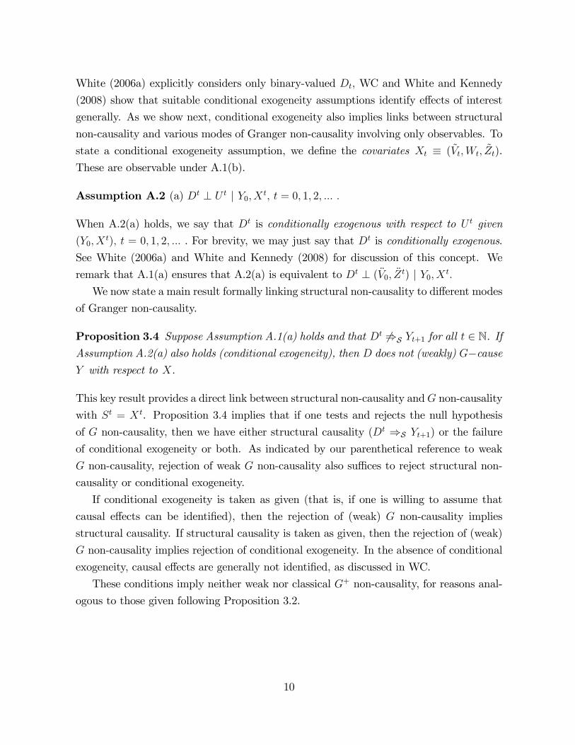
White (2006a) explicitly considers only binary-valued Dt; WC and White and Kennedy

(2008) show that suitable conditional exogeneity assumptions identify e¤ects of interest

generally. As we show next, conditional exogeneity also implies links between structural

non-causality and various modes of Granger non-causality involving only observables. To

state a conditional exogeneity assumption, we de�ne the covariates Xt � ( ~Vt;Wt; ~Zt).

These are observable under A.1(b).

Assumption A.2 (a) Dt ? U t j Y0; X t; t = 0; 1; 2; ::: :

When A.2(a) holds, we say that Dt is conditionally exogenous with respect to U t given

(Y0; Xt); t = 0; 1; 2; ::: . For brevity, we may just say that Dt is conditionally exogenous.

See White (2006a) and White and Kennedy (2008) for discussion of this concept. We

remark that A.1(a) ensures that A.2(a) is equivalent to Dt ? ( �V0; �Zt) j Y0; X t:

We now state a main result formally linking structural non-causality to di¤erent modes

of Granger non-causality.

Proposition 3.4 Suppose Assumption A.1(a) holds and that Dt 6)S Yt+1 for all t 2 N. IfAssumption A.2(a) also holds (conditional exogeneity), then D does not (weakly) G�causeY with respect to X.

This key result provides a direct link between structural non-causality andG non-causality

with St = X t. Proposition 3.4 implies that if one tests and rejects the null hypothesis

of G non-causality, then we have either structural causality (Dt )S Yt+1) or the failure

of conditional exogeneity or both. As indicated by our parenthetical reference to weak

G non-causality, rejection of weak G non-causality also su¢ ces to reject structural non-

causality or conditional exogeneity.

If conditional exogeneity is taken as given (that is, if one is willing to assume that

causal e¤ects can be identi�ed), then the rejection of (weak) G non-causality implies

structural causality. If structural causality is taken as given, then the rejection of (weak)

G non-causality implies rejection of conditional exogeneity. In the absence of conditional

exogeneity, causal e¤ects are generally not identi�ed, as discussed in WC.

These conditions imply neither weak nor classical G+ non-causality, for reasons anal-

ogous to those given following Proposition 3.2.

10

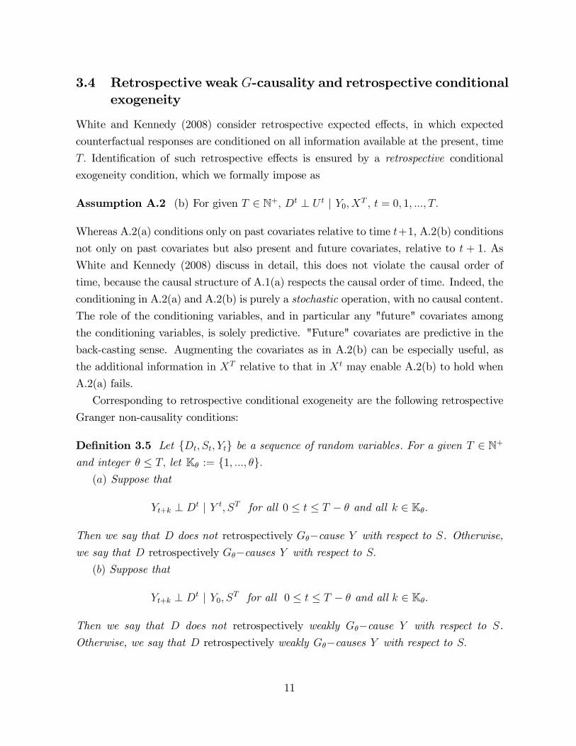
3.4 Retrospective weak G-causality and retrospective conditionalexogeneity

White and Kennedy (2008) consider retrospective expected e¤ects, in which expected

counterfactual responses are conditioned on all information available at the present, time

T: Identi�cation of such retrospective e¤ects is ensured by a retrospective conditional

exogeneity condition, which we formally impose as

Assumption A.2 (b) For given T 2 N+; Dt ? U t j Y0; XT ; t = 0; 1; :::; T:

Whereas A.2(a) conditions only on past covariates relative to time t+1, A.2(b) conditions

not only on past covariates but also present and future covariates, relative to t + 1: As

White and Kennedy (2008) discuss in detail, this does not violate the causal order of

time, because the causal structure of A.1(a) respects the causal order of time. Indeed, the

conditioning in A.2(a) and A.2(b) is purely a stochastic operation, with no causal content.

The role of the conditioning variables, and in particular any "future" covariates among

the conditioning variables, is solely predictive. "Future" covariates are predictive in the

back-casting sense. Augmenting the covariates as in A.2(b) can be especially useful, as

the additional information in XT relative to that in X t may enable A.2(b) to hold when

A.2(a) fails.

Corresponding to retrospective conditional exogeneity are the following retrospective

Granger non-causality conditions:

De�nition 3.5 Let fDt; St; Ytg be a sequence of random variables: For a given T 2 N+

and integer � � T; let K� := f1; :::; �g:(a) Suppose that

Yt+k ? Dt j Y t; ST for all 0 � t � T � � and all k 2 K�:

Then we say that D does not retrospectively G��cause Y with respect to S. Otherwise,

we say that D retrospectively G��causes Y with respect to S:

(b) Suppose that

Yt+k ? Dt j Y0; ST for all 0 � t � T � � and all k 2 K�:

Then we say that D does not retrospectively weakly G��cause Y with respect to S.

Otherwise, we say that D retrospectively weakly G��causes Y with respect to S:

11

The case where � = 1 is that most relevant here. For convenience, we thus refer to

retrospective (weak)G1 (non-) causality simply as retrospective (weak)G (non-) causality.

Just as for conditional exogeneity, there is no direct relation between weak and retro-

spective weak Granger (non-) causality. Neither is necessary nor su¢ cient for the other.

Nor are there any necessary relations between retrospective and classical Granger (non-)

causality.

We now state a main result formally linking structural non-causality to retrospective

(weak) Granger non-causality, parallel to Proposition 3.4.

Proposition 3.6 Suppose Assumption A.1(a) holds and that Dt 6)S Yt+1 for all t 2 N.If Assumption A.2(b) also holds (retrospective conditional exogeneity), then for the given

T; D does not retrospectively (weakly) G�cause Y with respect to X.

The structure wrovided by A.1(a) and A.2(b) thus implies both retrospective agd ret-

rospective weak G non-causality with ST = XT when Dt does not structurally cause

Yt+1:

3.5 Some converse results

So far, our results establish that given conditional exogeneity, structural non-causality

implies various forms of Granger non-causality. Our next result is a form of converse,

establishing that weak G non-causality implies a form of structural non-causality. To

establish this, we do not require conditional exogeneity; instead, we use a strengthened

version of structural causality.

Assumption A.3 For given t 2 N; suppose(a) there exist measurable sets BY ; B0; BD; and BX such that:

(i)

P [Yt+1 2 BY ; Y0 2 B0; Dt 2 BD; X t 2 BX ] > 0;

(ii)

P [Dt 2 BDjY0 2 B0; X t 2 BX ] < 1; and

(iii) with BU(dt; y0; xt) � supp(U t j Dt = dt; Y0 = y0; Xt = xt); for all dt =2 BD;

y0 2 B0; and xt 2 BX ; and all ut 2 BU(dt; y0; xt)

rt+1(y0; dt; ~vt; ~zt; �vt; �zt) 62 BY :

12

Observe that the requirement of A.3(a.i),

P [Yt+1 2 BY ; Y0 2 B0; Dt 2 BD; X t 2 BX ] > 0;

implies

P [Y0 2 B0; Dt 2 BD; X t 2 BX ] > 0 and P [Y0 2 B0; X t 2 BX ] > 0:

This in turn implies that

P [Dt 2 BD j Y0 2 B0; X t 2 BX ]= P [Y0 2 B0; Dt 2 BD; X t 2 BX ]=P [Y0 2 B0; X t 2 BX ]> 0:

Assumptions A.3(a.i) and A.3(a.ii) ensure 0 < P [Dt 2 BDjY0 2 B0; X t 2 BX ] < 1:Assumption A.3(a) is stronger than assuming that Dt)S Yt+1; because A.3(a) implies

Dt )S Yt+1; but Dt )S Yt+1 does not ensure A.3(a). In part, the idea is that the values

of the ancillary causes ensuring Dt )S Yt+1 may occur on a set with probability zero. If

so, we will not be able to detect structural causality in data. Assumption A.3(a) rules this

out. But Assumption A.3(a) goes further; it ensures that there are response values (those

in the set BY ) that can only be reached by variation in Dt; for some sets of conditioning

values of Y0 and X t (B0 and BX):

In fact, A.3(a) is quite a strong assumption. Consider, for example, the simple case

in which Yt = Dt + Ut; where Dt has unbounded support. Then A.3(a) can hold if the

support of Ut is conditionally bounded, but not otherwise. Because of its strength, this

condition may be plausible in some applications but not others. We o¤er A.3(a) and

the results that follow as a �rst step in investigating conditions ensuring that structural

causality implies G�causality. Despite its strength, A.3(a) nevertheless a¤ords usefulinsights, as discussed immediately below.

We provide a convenient way of referring to Assumption A.3(a) using the following

de�nition.

De�nition 3.7 (a) Suppose A.1 and A.3(a) hold. Then we say that Dt strongly causes

Yt+1 with respect to S, and we write Dt s)S Yt+1: Otherwise, we say that Dt does not

strongly cause Yt+1 with respect to S, and we write Dts

6)S Yt+1:

We can now state a form of converse to Proposition 3.4.

13

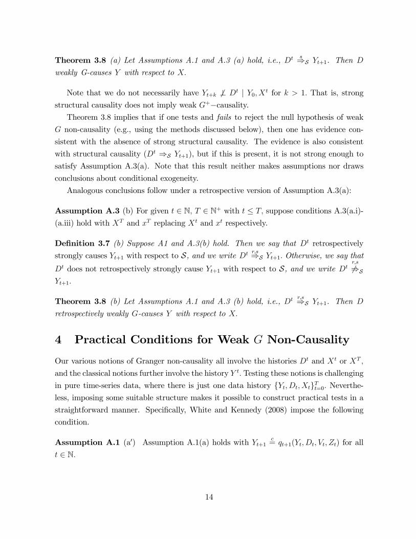
Theorem 3.8 (a) Let Assumptions A.1 and A.3 (a) hold, i.e., Dt s)S Yt+1. Then D

weakly G-causes Y with respect to X:

Note that we do not necessarily have Yt+k 6? Dt j Y0; X t for k > 1: That is, strong

structural causality does not imply weak G+�causality.Theorem 3.8 implies that if one tests and fails to reject the null hypothesis of weak

G non-causality (e.g., using the methods discussed below), then one has evidence con-

sistent with the absence of strong structural causality. The evidence is also consistent

with structural causality (Dt )S Yt+1), but if this is present, it is not strong enough to

satisfy Assumption A.3(a). Note that this result neither makes assumptions nor draws

conclusions about conditional exogeneity.

Analogous conclusions follow under a retrospective version of Assumption A.3(a):

Assumption A.3 (b) For given t 2 N; T 2 N+ with t � T; suppose conditions A.3(a.i)-

(a.iii) hold with XT and xT replacing X t and xt respectively.

De�nition 3.7 (b) Suppose A1 and A.3(b) hold. Then we say that Dt retrospectively

strongly causes Yt+1 with respect to S, and we write Dt r;s)S Yt+1: Otherwise, we say that

Dt does not retrospectively strongly cause Yt+1 with respect to S, and we write Dtr;s

6)S

Yt+1:

Theorem 3.8 (b) Let Assumptions A.1 and A.3 (b) hold, i.e., Dt r;s)S Yt+1. Then D

retrospectively weakly G-causes Y with respect to X:

4 Practical Conditions for Weak G Non-Causality

Our various notions of Granger non-causality all involve the histories Dt and X t or XT ;

and the classical notions further involve the history Y t: Testing these notions is challenging

in pure time-series data, where there is just one data history fYt; Dt; XtgTt=0: Neverthe-less, imposing some suitable structure makes it possible to construct practical tests in a

straightforward manner. Speci�cally, White and Kennedy (2008) impose the following

condition.

Assumption A.1 (a0) Assumption A.1(a) holds with Yt+1c= qt+1(Yt; Dt; Vt; Zt) for all

t 2 N:

14

Assumption A.1(a0) imposes "�rst order" dynamic structure on the data generating process

for fYtg: Analogous results hold with any �nite order dynamic structure, but we consider�rst order structure for concreteness and clarity.

To state the next assumption, let dFt+1;t( � jyt; dt; xt) denote the conditional densityof Yt+1 given Yt = yt; Dt = dt; and X t = xt; and let dF�� ( � jyt; dt; xtt�� ) denote theconditional density of Yt+1 given Yt = yt; Dt = dt; and X t

t�� = xtt�� ; where Xtt��

(Xt�� ; :::; Xt) is the one-sided (��) near history of Xt. Similarly, let dFt+1;T ( � jyt; dt; xT )denote the conditional density of Yt+1 given Yt = yt; Dt = dt; and XT = xT ; and let

dF� ( � jyt; dt; xt+�t�� ) denote the conditional density of Yt+1 given Yt = yt; Dt = dt; and

X t+�t�� = xt+�t�� ; where X

t+�t�� (Xt�� ; :::; Xt+� ) is the two-sided (��) near history of Xt.

Assumption A.4(a) There exist � 2 N and a conditional density dF�� such that for all t 2 N and for

all argument values

dFt+1;t(yt+1jyt; dt; xt) = dF�� (yt+1jyt; dt; xtt�� ):

(b) There exist � 2 N and a conditional density dF� such that for given T 2 N+; allintegers t � T � � , and for all argument values

dFt+1;T (yt+1jyt; dt; xT ) = dF� (yt+1jyt; dt; xt+�t�� ):

Assumption A.4 combines a memory condition with a conditional stationarity assumption.

The memory condition says that only the near history X tt�� (X

t+�t�� ) of the covariates is

useful in predicting the response Yt+1, given Yt and Dt: The fact that dF�� (dF� ) does

not have a subscript t expresses the assumption that the conditional density is the same

for all t, thereby imposing conditional stationarity. Observe that conditional stationarity

does not rule out integrated or cointegrated processes.

For the retrospective case, White and Kennedy (2008) establish a recursive representa-

tion of dFt+1;T (yt+1 j y0; dt; xT ): We state a version of this in our next result (Proposition4.1(b)). To obtain a similar representation for dFt+1;t(yt+1 j y0; dt; xt), we impose onefurther assumption.

Assumption A.5 Yt ? Xt j Y0; Dt�1; X t�1; t = 0; 1; 2; ::: :

This assumption is not implied by our prior assumptions, but it is nevertheless plausible

given that the elements of Xt do not enter the structural equation for Yt under A.1(a0).

15

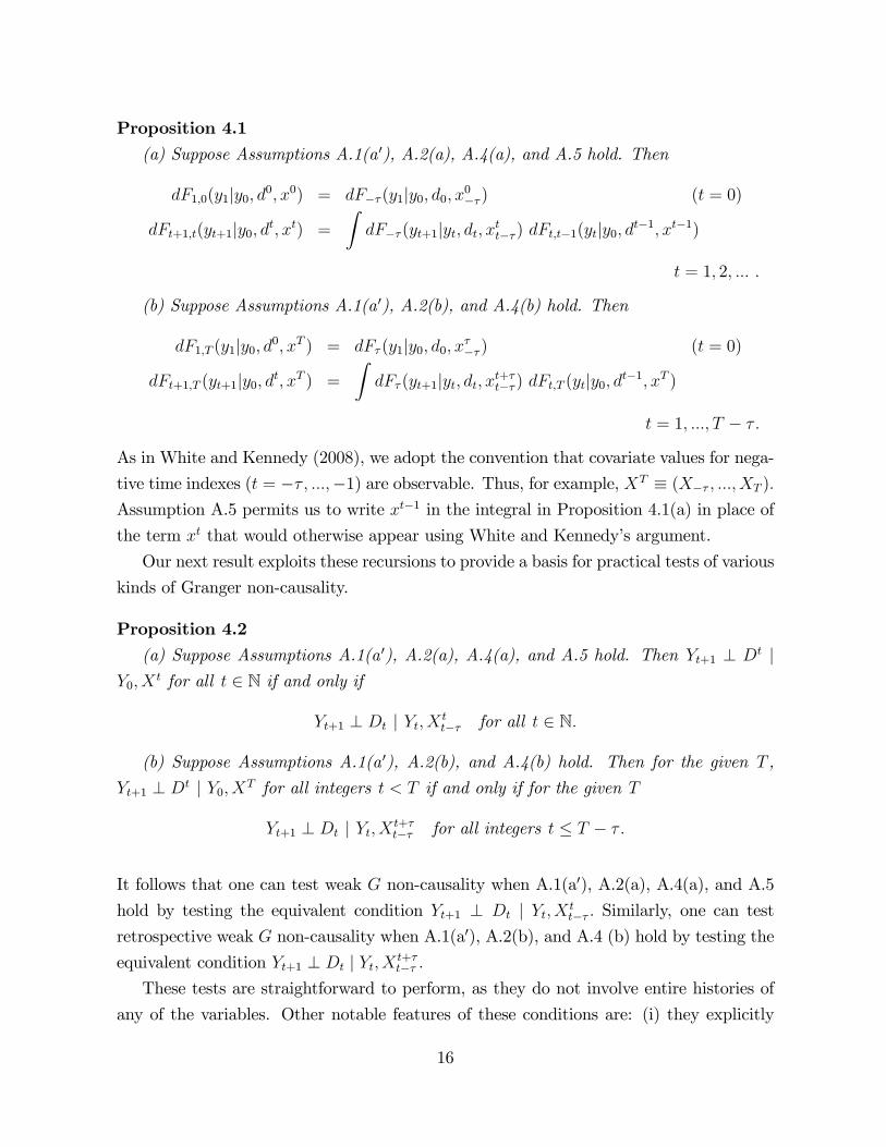
Proposition 4.1(a) Suppose Assumptions A.1(a 0), A.2(a), A.4(a), and A.5 hold. Then

dF1;0(y1jy0; d0; x0) = dF�� (y1jy0; d0; x0�� ) (t = 0)

dFt+1;t(yt+1jy0; dt; xt) =

ZdF�� (yt+1jyt; dt; xtt�� ) dFt;t�1(ytjy0; dt�1; xt�1)

t = 1; 2; ::: :

(b) Suppose Assumptions A.1(a 0), A.2(b), and A.4(b) hold. Then

dF1;T (y1jy0; d0; xT ) = dF� (y1jy0; d0; x�� ) (t = 0)

dFt+1;T (yt+1jy0; dt; xT ) =

ZdF� (yt+1jyt; dt; xt+�t�� ) dFt;T (ytjy0; dt�1; xT )

t = 1; :::; T � � :

As in White and Kennedy (2008), we adopt the convention that covariate values for nega-

tive time indexes (t = �� ; :::;�1) are observable. Thus, for example, XT � (X�� ; :::; XT ):

Assumption A.5 permits us to write xt�1 in the integral in Proposition 4.1(a) in place of

the term xt that would otherwise appear using White and Kennedy�s argument.

Our next result exploits these recursions to provide a basis for practical tests of various

kinds of Granger non-causality.

Proposition 4.2(a) Suppose Assumptions A.1(a 0), A.2(a), A.4(a), and A.5 hold. Then Yt+1 ? Dt j

Y0; Xt for all t 2 N if and only if

Yt+1 ? Dt j Yt; X tt�� for all t 2 N:

(b) Suppose Assumptions A.1(a 0), A.2(b), and A.4(b) hold. Then for the given T ,

Yt+1 ? Dt j Y0; XT for all integers t < T if and only if for the given T

Yt+1 ? Dt j Yt; X t+�t�� for all integers t � T � � :

It follows that one can test weak G non-causality when A.1(a0), A.2(a), A.4(a), and A.5

hold by testing the equivalent condition Yt+1 ? Dt j Yt; X tt�� : Similarly, one can test

retrospective weak G non-causality when A.1(a0), A.2(b), and A.4 (b) hold by testing the

equivalent condition Yt+1 ? Dt j Yt; X t+�t�� :

These tests are straightforward to perform, as they do not involve entire histories of

any of the variables. Other notable features of these conditions are: (i) they explicitly

16

specify which conditioning variables to include, namely a near history of the covariates;

(ii) the retrospective version includes leads as well as lags of the covariates.

There are numerous methods for testing the conditional independence identi�ed in

Proposition 4.2. For example, one can apply nonparametric methods of Su and White

(2007a, 2007b, 2008). Nevertheless, because of the typically modest number of time series

observations available relative to the number of relevant observable variables, parametric

methods for testing conditional independence will usually be more practical. In the ap-

plications of Section 6, we illustrate how parametric methods similar to those proposed

in section 5 of White (2006a) can be exploited to obtain tests with useful power against

a wide range of departures from conditional independence.

5 Testing (Retrospective) Conditional Exogeneity

Our main results in Section 3 crucially involve either conditional exogeneity or retro-

spective conditional exogeneity. In this section we provide some discussion about how to

choose covariates to help ensure these conditions, and we provide results supporting tests.

For concreteness, consider conditional exogeneity, the property that Dt ? U t j Y0; X t:

As explained in White (2006a), covariates Xt should include variables that are useful for

predicting either Dt or U t; as the better a predictor Xt is, the less useful Dt will be as a

predictor for U t and vice-versa. By applying Reichenbach�s (1956) principle of common

cause (if X and Y are correlated, then either X causes Y, Y causes X , or there is anunderlying common cause, say Z), White (2006a) reasons that Xt should include: (1)

observable causes ~Vt and ~Zt of Yt+1; (2) observable causes ~Vt;Wt; and ~Zt of Dt+1; and

(3) observable responses Wt to unobservable causes Ut of Yt+1 and/or Dt+1. In the case

of retrospective conditional exogeneity, the latter class of variables justi�es inclusion of

leads of ~Vt;Wt; and ~Zt:

Although economic theory can play a key role in justifying conditional exogeneity, it

is desirable to have straightforward statistical methods for empirically testing whether

a given Xt delivers (retrospective) conditional exogeneity. White (2006a) and White

and Chalak (2007c) provide a variety of tests for conditional exogeneity. White (2006a)

considers time-series conditional exogeneity tests where Dt is a binary variable. White

and Chalak (2007c) provide tests for cross-section data. Here we take a similar approach

appropriate for our general dynamic structure.

17

5.1 Testing conditional exogeneity

A �rst challenge in testing conditional exogeneity is that Ut is unobservable. A result

of White and Chalak (2007c) permits us to overcome this by delivering a consequence

of conditional exogeneity that involves only observables, provided that one can observe

suitable additional proxies. Assumption A.6(a) describes these additional variables.

Assumption A.6 (a) There exists an observable k ~w � 1 random vector ~W0; with k ~w�nite and positive, and an unobservable sequence of k�u� 1 random vectors f �Utg, with k�ua countably valued integer, such that (i) f ~Wtg is generated as

~Wt+1c= b3;t+1( ~W

t; X t; U t; �U t); t = 0; 1; :::;

where b3;t+1 is an unknown measurable function of dimension k ~w; and (ii)

Dt ? ( �U t; ~W0) j Y0; U t; X t; t = 1; 2; ::: :

A leading example is the case in which ~Wt+1 is an error-laden version of Ut, e.g., ~Wt+1 =

w(Ut) + �Ut: When �Ut is a measurement error, Assumption A.6(a.ii) is quite plausible.

We also impose an assumption on the initial values Y0 and ~W0 that permits us to

remove Y0 from the conditioning information set.

Assumption A.7 (a) ( ~Wt+1; ~Wt) ? ( ~W0; Y0) j X t for all t = 1; 2; ::: .

Assumption A.7(a) imposes a plausible restriction on the usefulness of the initial values

of ( ~W0; Y0) for predicting ~Wt and ~Wt+1; given X t:

Tests for conditional exogeneity based solely on observables follow from our next result.

Proposition 5.1 (a) Suppose Assumptions A.1(a), A.6(a), and A.7(a) hold. Then Dt ?U t j Y0; X t for all t 2 N implies ~Wt+1 ? Dt j ~W0; X

t for all t 2 N.

As in the case of weak G non-causality, it is inconvenient to attempt to test conditions

that involve entire data histories (here, Dt and X t): Nevertheless, an assumption similar

to A.4(a) delivers results similar to those of Proposition 4.2(a), supporting convenient

tests for conditional exogeneity that involve only �nite data histories. For this we let

dFt+1;t( ~wt+1 j ~wt; dt; xt) de�ne the conditional density of ~Wt+1 given ~Wt = ~wt; Dt = dt;

and X t = xt; and we let dF�� ( ~wt+1 j ~wt; dt; xtt�� ) de�ne the conditional density of ~Wt+1

given ~Wt = ~wt; Dt = dt; and X tt�� = xtt�� .

18

Assumption A.8 (a) There exists a �nite non-negative integer � such that for all t 2 N,and for all argument values

dFt+1;t( ~wt+1j ~wt; dt; xt) = dF�� ( ~wt+1j ~wt; dt; xtt�� ):

We also impose an assumption analogous to A.5.

Assumption A.9 For all t 2 N+; ~Wt ? Xt j ~W0; Xt�1:

A.9 is plausible, as Xt does not enter the structural equation for ~Wt:

The next result supports conditional exogeneity tests that involve only a �nite number

of lags of Xt.

Proposition 5.2 (a) Suppose Assumptions A.1(a), A.6(a), A.7(a), A.8(a), and A.9 hold.Then ~Wt+1 ? Dt j ~W0; X

t for all t 2 N if and only if ~Wt+1 ? Dt j ~Wt; Xtt�� for all t 2 N:

Thus, rejecting ~Wt+1 ? Dt j ~Wt; Xtt�� implies rejecting conditional exogeneity, D

t ? U t jY0; X

t: Just as for (weak) G non-causality tests, one may apply either parametric or

non-parametric tests of the conditional independence hypothesis ~Wt+1 ? Dt j ~Wt; Xtt�� .

5.2 Testing retrospective conditional exogeneity

Results for retrospective conditional exogeneity analogous to those of the previous sub-

section hold under analogous conditions. The notation in Assumption A.8(b) is parallel

to that previously de�ned.

Assumption A.6 (b) Assumption A.6(a.i) holds; and (ii) for given �nite integer T ,

Dt ? ( �U t; ~W0) j Y0; U t; XT ; t = 1; 2; :::; T:

Assumption A.7 (b) ( ~Wt+1; ~Wt) ? ( ~W0; Y0) j XT for all t = 1; 2; :::; T � 1:

Proposition 5.1 (b) Suppose Assumptions A.1(a), A.6(b), and A.7(b) hold. Then Dt ?U t j Y0; XT for all t = 0; 1; :::; T implies ~Wt+1 ? Dt j ~W0; X

T for all t = 0; 1; :::; T � 1:

Assumption A.8 (b) There exists a �nite non-negative integer � such that for given Tand all integers t � T � � , and for all argument values

dFt+1;T ( ~wt+1j ~wt; dt; xT ) = dF� ( ~wt+1j ~wt; dt; xt+�t�� ):

19

Proposition 5.2 (b) Suppose Assumptions A.1(a), A.6(b), A.7(b), and A.8(b) hold.Then for given T; ~Wt+1 ? Dt j ~W0; X

T for all integers t < T if and only if ~Wt+1 ? Dt j~Wt; X

t+�t�� for all integers t � T � � :

Observe that we do not require A.9 here. Parallel to the previous case, rejecting ~Wt+1 ? Dt

j ~Wt; Xt+�t�� implies rejecting retrospective conditional exogeneity, D

t ? U t j Y0; XT :

5.3 A pure test of structural non-causality

Our results of Section 3 say that if we reject (weak) G non-causality, then we must reject

either structural non-causality or conditional exogeneity (or both). The results just given

provide a way to test conditional exogeneity. If we �nd that we reject G non-causality

but not conditional exogeneity, then we have evidence against structural non-causality.

We thus propose a simple formal test of structural non-causality:

Reject structural non-causality if the (retrospective) (weak) G non-causality

test rejects and the (retrospective) conditional exogeneity test fails to reject.

Our next result provides easy bounds on the level and power of this test.

Proposition 5.3 Suppose the signi�cance levels of the (retrospective) conditional ex-

ogeneity test, the (retrospective) (weak) G non-causality test, and the structural non-

causality test are �1; �2; and � respectively. Suppose the powers of the (retrospective)

conditional exogeneity test, the (retrospective) (weak) G non-causality test, and the struc-

tural non-causality test are �1; �2; and � respectively. Then

max f0;min f(�2 � �1) ; (�2 � �1) ; (�2 � �1)gg �� maxfminf1� �1; �2g;minf1� �1; �2g;minf1� �1; �2gg and

�2 � �1 � � � min f1� �1; �2g :

The intuition here is that the level of the structural non-causality test decreases with the

level of the G non-causality test and the power of the conditional exogeneity test. The

lower bound for the level is zero when �1 is su¢ ciently large. For the power, the intuition

is that the power of the structural non-causality test increases with the power of the G

non-causality test and decreases with the level of the conditional exogeneity test.

20

In applications, tests are usually conducted using asymptotic critical values. The exact

level and power of a given test is then unknown, but it nevertheless converges to a known

limit. When the conditional exogeneity and G non-causality tests are consistent, as can

often be arranged, we have the following properties for the asymptotic level and power of

our procedure. (Limits are taken as T !1:)

Proposition 5.4 Suppose that for T = 1; 2; ::: the signi�cance levels of the (retrospec-

tive) conditional exogeneity test, the (retrospective) (weak) G non-causality test, and the

structural non-causality test are �1T ; �2T ; and �T respectively, and that �1T ! �1 and

�2T ! �2: Suppose the powers of the (retrospective) conditional exogeneity test, the (ret-

rospective) (weak) G non-causality test, and the structural non-causality test are �1T ; �2T ;

and �T respectively, and that �1T ! 1 and �2T ! 1. Then

0 � lim inf �T � lim sup�T � minf1� �1; �2g and �T ! 1� �1:

Typically, we can achieve �1 = 0 and �2 = 0 for a consistent test by suitable choice of

an increasing sequence of critical values. In this case we also have �T ! 0 and �T ! 1:

We note that conditional exogeneity tests may or may not be consistent against every

possible alternative. When the DGP corresponds to an alternative for which unit power

is not achieved, a weaker bound on the level and power of structural non-causality test

still holds by Proposition 5.3. This suggests exercising care to design the conditional

exogeneity test to be consistent against particularly important or plausible alternatives.

6 Illustrative Applications

In this section, we illustrate our methods by studying structural causality in industrial

pricing, macroeconomics, and �nance. First, we investigate structural causality from

crude oil prices to gasoline prices. Second, we examine structural causality from monetary

policy to industrial production. Third, we investigate structural causality from expected

macroeconomic announcements to stock returns.

6.1 Test Implementation

To test (retrospective) weak G non-causality and (retrospective) conditional exogeneity,

we require tests for conditional independence. Non-parametric tests for conditional inde-

pendence consistent against arbitrary alternatives are readily available (e.g., Linton and

21

Gozalo, 1997; Fernandes and Flores, 2001; Delgado and Gonzalez-Manteiga, 2001; and

Su and White, 2007a, 2007b, 2008), but given the large number of covariates in most

applications, these are often not practical. Here we apply parametric tests designed to

have power against a relatively broad spectrum of alternatives. Speci�cally, we apply

both traditional linear parametric tests and new, more �exible parametric tests based on

the "QuickNet" procedures introduced by White (2006b).

6.1.1 Testing conditional mean independence with linear conditional expec-tations

Traditional tests of G non-causality are based on the fact that rejection of conditional

mean independence implies rejection of conditional independence. Tests of conditional

mean independence are typically implemented by assuming the linearity of the conditional

expectation. Accordingly, to test Y ? D j S, we �rst suppose that

E(Y j D;S) = �+D0�0 + S 0�1:

Under the null that Y ? D j S; we have �0 = 0: Thus, we estimate the coe¢ cients of thefollowing regression equation and test �0 = 0 :

Y = �+D0�0 + S 0�1 + ": (CI Test Regression 1)

If we reject �0 = 0, then we also reject Y ? D j S: On the other hand, if we fail toreject �0 = 0, this does not necessarily imply a failure to reject Y ? D j S; as conditionalindependence can easily fail even if conditional mean independence holds.

6.1.2 Testing conditional mean independence with �exible conditional expec-tations

To achieve power against a wider range of alternatives than the traditional linear method

just speci�ed, we can use a more �exible function to test conditional mean independence.

In particular, we consider a speci�cation exploited in White�s (2006b, p.476) QuickNet

procedure:

E(Y j D;S) = a+D0�0 + S 0�1 +qXj=1

(S 0 j)�j+1;

where is a given activation function belonging to the class of generically comprehensively

revealing (GCR) functions. Here we let be the logistic cdf (z) = 1=(1 + exp(�z)) orthe ridgelet function (z) = (�z5 + 10z3 � 15z) exp(�:5z2) (see, for example, Candès,

22

1999). We call (S 0 j) the "activation" of "hidden unit" j. The integer q lies between 1and �q; the maximum number of hidden units. We choose j according to the algorithm

proposed in White (2006b, p.477). Thus, we estimate the coe¢ cients of the following

regression equation and test �0 = 0:

Y = a+D0�0 + S 0�1 +qXj=1

(S 0 j)�j+1 + ": (CI Test Regression 2)

6.1.3 Testing conditional independence using non-linear transformations

Third, to gain power against alternatives for which conditional mean independence holds

but conditional independence fails, we consider tests based on transformations of Y andD, as Y ? D j S implies that y(Y) ? d(D) j S for all measurable functions y and d:Accordingly, we consider speci�cations of the form

E( y(Y) j d(D);S) = a+ d(D)0�0 + S 0�1 +qXj=1

(S 0 j)�j+1:

We let y and d be the logistic cdf or ridgelet functions. The choices of ; q; and

are the same as in the previous case. Thus, we estimate the coe¢ cients of the following

regression equation and test �0 = 0 :

y(Y) = a+ d(D)0�0 + S 0�1 +qXj=1

(S 0 j)�j+1 + ": (CI Test Regression 3)

6.2 Crude oil and gasoline prices

White and Kennedy (2008) apply their methods for estimating retrospective causal e¤ects

to study the impact of crude oil prices on gasoline prices. Our methods here are fully

applicable to this setting. We let the response of interest, Yt; be the natural logarithm of

the spot price for US Gulf Coast conventional gasoline; our cause of interest, Dt; is the

natural logarithm of the Cushing OK WTI spot crude oil price. We let Ut represent all

unobservable causes of gasoline prices, so that ~Vt and ~Zt have zero dimension, as in White

and Kennedy (2008).

Considering that crude oil prices should be quickly re�ected in gasoline prices (e.g.,

as found by Borenstein, Cameron, and Gilbert, 1997) and that our data frequency is

monthly, a relatively long interval, here we investigate the structural causality of Dt on

contemporaneous Yt. Thus, we take the structure of interest to be

Ytc= rt(Y0; D

t; U t); t = 0; 1; :::; T:

23

We view this as involving "contemporaneous" rather than "instantaneous" causation. We

distinguish these notions as follows. For contemporaneous causation, the cause precedes

the response, but the causal interval is less than the observational interval. Thus, the

causal response occurs within the observed interval, justifying the appearance of the

contemporaneous value of a potential cause in the structural relation. On the other hand,

instantaneous causation violates the principle that causes precede e¤ects. We rule this

out.

We do not explicitly treat contemporaneous causation in our theoretical analysis above,

but all the relevant results hold by replacing Yt+1 with Yt on the left-hand side of the

implicit dynamic response function, and similarly in the other implicit dynamic relations.

This structure is that explicitly analyzed by White and Kennedy (2008).

Let Wt be proxies for the unobservable causes Ut. Similar to White and Kennedy

(2008), we let Wt include (1) the natural logarithm of Texas Initial and Continuing Un-

employment Claims (taken from State Weekly Claims for Unemployment Insurance Data,

Not Seasonally Adjusted); (2) Houston temperature; (3) a winter dummy for January,

February, and March; (4) a summer dummy for June, July, and August; (5) the nat-

ural logarithm of U.S. Bureau of Labor Statistics Electricity price index; (6) the 10-Year

Treasury Note Constant Maturity Rate; (7) the 3-Month T-Bill Secondary Market Rate;

and (8) the Index of the Foreign Exchange Value of the Dollar. Here, the covariates are

Xt = Wt: Our sample period covers from January 1987 through December 1997, a total

132 observations.

Over our sample period, both crude oil and gasoline prices are relatively stable. Specif-

ically, the augmented Dickey-Fuller tests for stationarity of Yt and Dt reject the null

hypothesis that these series contain a unit root. Nevertheless, we cannot reject the hy-

pothesis that there is a unit root for certain of the covariates (the 10-year Treasury Note

rate, the 3-month T-Bill rate, the natural logarithm of the electricity price index, and

the index of the foreign exchange value of the dollar). We enter these covariates in �rst

di¤erences.

There are some di¤erences between our use of data and that of White and Kennedy

(2008): (1) The sample period is di¤erent; (2) The natural gas price index does not appear

in Wt; instead we include this in ~Wt below; (3) We use the Federal Reserve�s Index of the

Foreign Exchange Value of the Dollar instead of the Yen-US dollar and British pound-US

dollar exchange rates to avoid multicollinearity (see http://www.federalreserve.gov/releases/

h10/summary/); and (4) Here, we consider a stationary process with contemporaneous

causation, whereas White and Kennedy�s (2008) empirical analysis involves a cointegrated

24

relation with a one period lag.

To test structural non-causality, we apply the procedure of Section 5.3. Speci�cally, we

perform tests of the key retrospective conditional exogeneity assumption, Dt ? U tjY0; XT ;

together with tests for retrospective weak G non-causality.

To test retrospective conditional exogeneity, we let ~Wt be the natural logarithm of the

U.S. Bureau of Labor Statistics Natural Gas Price Index. The key requirement for ~Wt is

A.6(b). Allowing contemporaneous causation, we state A.6 (b.i) as

~Wtc= b3;t( ~W

t�1; X t; U t; �U t);

where �Ut represents additional unobservable drivers of ~Wt other than Ut: This is a plausible

assumption, as we may view ~Wt as an error-laden measure of the natural gas prices that

actually drive oil prices, a component of Ut: The measurement error is then �Ut: Assumption

A.6 (b.ii) is the condition that

Dt ? ( �U t; ~W0) j Y0; U t; XT :

This condition means that conditioning on all the unobservable causes of gasoline prices

and the covariates, crude oil prices are independent of the measurement error history �U t

and the initial value of the natural gas price index, ~W0: This is also reasonably plausible.

With suitable memory and conditional stationarity assumptions as speci�ed in Sec-

tion 5, we test retrospective conditional exogeneity by testing Dt ? ~Wt j ~Wt�1; Xt+�t�� .

We implement the tests in the three forms (CI Test Regressions 1-3) described above.

Speci�cally, we let Y = ~Wt; D = Dt, and S = ( ~Wt�1; Xt+�t�� ); and we test �0 = 0: Given

the relatively small sample size, we consider only � � 5.We report our results in Tables 1-3. For CI Test Regression 1, we cannot reject �0 = 0

for all � = 1; 2; :::; 5 at the 5% signi�cance level. For CI Test Regression 2, we take �q � 5.Letting be the ridgelet function, we again cannot reject �0 = 0 for all � and q at the

5% signi�cance level: If we let function be the logistic cdf, we cannot reject �0 = 0

for most values of � and q: Exceptions are for � = 2 and q = 2; 3; 4 or 5; however, the

Bonferroni-Hochberg p-value bounds for the rows and columns and for the table as a

whole do not support rejection. For CI Test Regression 3, we again cannot reject �0 = 0

for almost all the choices of � ; q; ; ~w; and d: For brevity, we report results only for

the ridgelet case. Taken together, our results suggest that we cannot reject retrospective

conditional exogeneity.

For comparison purposes, we also implemented a (non-retrospective) conditional exo-

geneity test of the hypothesis Dt ? ~Wt j ~Wt�1; Xtt�� ; again using CI Test Regressions 1-3:

25

The results are quite similar: we again cannot reject conditional exogeneity. Given the

similarity of the results, to save space we report only the results for CI Test Regression 1

(see Table 1).

Next, we implement retrospective weak G non-causality tests. With suitable memory

and conditional stationarity assumptions as speci�ed in Section 4, we can test retrospec-

tive weak G non-causality by testing Yt ? Dt j Yt�1; X t+�t�� : We implement the tests in the

three forms described above. Speci�cally, we let Y = Yt; D = Dt, and S = (Yt�1; X t+�t�� );

and we test �0 = 0: Tables 4-6 contain the results. As expected, we soundly reject �0 = 0

for all three regressions and for all choices of � ; q; ; y; and d: As a comparison, we

also implement (non-retrospective) weak G non-causality tests. The results are similar;

again we soundly reject �0 = 0 for all the three regressions. To save space, we report

these results only in Table 4.

Given the consistency of our tests for retrospective conditional exogeneity, Proposi-

tion 5.4 ensures that we can soundly reject the hypothesis of structural non-causality

from crude oil prices to contemporaneous gasoline prices. Interestingly, when we replace

contemporaneous crude oil prices with lagged crude oil prices, the results become much

more equivocal, suggesting that contemporaneous causation plays a central role in this

market. For brevity, we do not tabulate these results here.

6.3 Monetary policy and industrial production

Angrist and Kuersteiner (2004) study the causal relationship between the Federal Re-

serve�s monetary policy and output using the data from Romer and Romer (1989). Romer

and Romer (1989, 1994) construct a monetary policy shock variable using a narrative ap-

proach. They examine the Federal Open Market Committee minutes to identify dates

when the Fed took a marked anti-in�ationary stance. There are six such dates over the

period from 1948 through 1991 (Romer and Romer 1994), the "Romer dates." The total

number of observations is 528.

Our methods are applicable to this setting. As in Angrist and Kuersteiner (2004),

we let the response of interest (Yt) be industrial production growth and the cause of

interest (Dt) be the Fed�s anti-in�ationary stance as measured by the Romer dates. The

observable ancillary causes ( ~Zt) are unemployment and in�ation rates, and Ut represents

unobservable causes. Wt and ~Vt are empty, so here the covariates are Xt = ~Zt. Industrial

production is thus determined as

Yt+1c= rt+1(Y0; D

t; ~Zt; U t); t = 0; 1; :::; T:

26

The null hypothesis is that monetary policy has no causal e¤ect on the real economy.

Under this null, not only does Dt not structurally cause Yt+1; but it also does not struc-

turally cause ~Zt or U t: This system thus satis�es the recursivity required by Assumption

A.1.

Signi�cantly, this structure also justi�es the key retrospective conditional exogeneity

assumption, Dt ? U t j XT : This condition says that given XT ; U t cannot help predict

Dt; and vice versa. Put another way, given past and future unemployment and in�ation

rates, the Fed�s policy is as good as randomly assigned. Fed decisions usually target future

in�ation and/or unemployment rates. To the extent that expectations about these targets

are driven by past and present values of unemployment and in�ation, current and lagged

values of Xt should predict Dt well, leaving little role for U t in predicting Dt: Even when

the null is true, so that Dt has no impact on future values of Xt; those future values may

be driven by U t: Leads of Xt may thus be useful in back-casting U t; leaving little role

for Dt in predicting U t. Both of these features act to ensure Dt ? U t j XT : Moreover,

when the null is false, so that Dt does impact future values of Xt; leads of Xt will act to

back-cast Dt; again reducing any role of U t in predicting Dt.

An important criticism of Romer and Romer�s (1989) approach is that it neglects the

forward-looking aspects of monetary policy (e.g., Shapiro, 1994; Leeper, 1997). By appro-

priately conditioning on both leads and lags of covariates, we exploit rather than neglect

the forward-looking aspects of monetary policy. This makes the use of our retrospective

approach especially appealing.

These structural considerations justify taking retrospective conditional exogeneity to

be given here. Testing structural non-causality can now be accomplished by testing ret-

rospective weak G non-causality. With suitable memory and conditional stationarity

conditions, as speci�ed in Section 4, we test this by testing Yt+1 ? Dt j Yt; X t+�t�� : We run

the three CI test regressions described above; speci�cally, we let Y = Yt+1; D = Dt; and

S = (Yt; X t+�t�� ) and test �0 = 0; letting the maximum � equal 12. For CI Test Regression

1, we �nd that we cannot reject �0 = 0; no matter how we choose � : The results are

reported in Table 7. For CI Test Regression 2, we let the maximum q equal 9 and we

again �nd that �0 is insigni�cant for all � . Representative results are reported in Table

8. For CI Test Regression 3, again we �nd that �0 is insigni�cant for most choices of � ;

q; ; y and d: Representative results are reported in Table 9.

For comparison, we test weak G non-causality conditioning only on covariate lags, i.e.,

we test Yt+1 ? Dt j Yt; X tt�� : For CI Test Regression 1, we �nd that �0 is insigni�cant

when � < 4 and signi�cant when � � 4: These results are reported in Table 7. For CI

27

Test Regressions 2 and 3, the results are the same as in the retrospective case: we cannot

reject �0 = 0. We omit tabulating these results to save space.

Before concluding that there is no evidence against the null that monetary policy has

no real impacts, we must consider the possibility that the e¤ects of monetary policy take

more than one month to be felt. Thus, we relax the single lag assumption of Section 4,

and we now permit monetary policy over the past year (Dtt�12) to possibly impact the

current growth of industrial production. We continue to assume retrospective conditional

exogeneity. Under the null of no structural causality, we then have Yt+1 ? Dtt�12 j Yt; X t+�

t�� :

We again run the three CI test regressions, but now with Y = Yt+1; D = Dtt�12; and

S = (Yt; X t+�t�� ); and we test �0 = 0 jointly. For all three CI test regressions, we soundly

reject �0 = 0. Representative results are reported in Tables 10-12.

For comparison, we also condition only on lags of covariates, i.e., we test Yt+1 ? Dtt�12 j

Yt; Xtt�� : Again we reject �0 = 0. The results of CI Test Regression 1 are reported in Table

10. The results of Regressions 2 and 3 are the same; we omit these to save space.

Our results suggest that we can soundly reject the hypothesis that monetary policy

has no causal e¤ects on the real economy if we permit the e¤ects of monetary policy

to gradually �lter into the real economy. This is consistent with Romer and Romer�s

(1989, 1994) conclusion that "these [monetary] policy shifts were followed by large and

statistically signi�cant declines in real output relative to its usual behavior. We interpret

these results as supporting the view that monetary policy has substantial real e¤ects." On

the other hand, our results contrast with Angrist and Kuersteiner�s (2004) conclusions;

they �nd that "money-output causality can fairly be described as mixed."

6.4 Stock returns and macroeconomic announcements

Beginning with Chen, Roll, and Ross (1986), many authors have studied the impact

of macroeconomic factors on aggregate stock returns (see, e.g., Flannery and Protopa-

padakis, 2002). In this section, we investigate whether there are causal e¤ects from

expected economic announcements to stock returns. This is in part a test of market

weak e¢ ciency, because if stock markets are e¢ cient in the weakest sense, then expected

returns should not respond to expected economic announcements. On the other hand,

other moments of the returns distribution may be a¤ected by expected announcements

without violating market weak e¢ ciency.

Although it would also be interesting to examine the causal e¤ects of economic news

(unexpected announcements) on stock returns, it is not obvious how one might justify

28

(retrospective) conditional exogeneity for news. We therefore leave an investigation of the

e¤ects of news to other work.

We let Yt; Dt; and ~Vt denote stock market returns, expected economic announcements,

and economic news, respectively; and we let Ut denote unobservable causes. The structural

relation is thus

Yt+1c= rt+1(Y0; D

t; ~V t; U t); t = 0; 1; :::; T

The sample consists of daily data from January 5, 1995 through October 31, 2006.

The daily returns series is that for the value-weighted NYSE-AMEX-NASDAQ market

index from the Center for Research on Security Prices (CRSP).

We decompose macroeconomic announcements into economic news and expected changes.

For example, let At denote a macroeconomic announcement at time t and let Et denote

its expectation. Then At �At�1 = (At �Et) + (Et �At�1) = ~Vt +Dt; ~Vt = At �Et then

represents news and Dt = Et � At�1 represents the expected change.

Here we include eight major macroeconomic announcements: (1) real GDP (ad-

vanced); (2) core CPI; (3) core PPI; (4) unemployment rate; (5) new home sales; (6)

nonfarm payroll employment; (7) consumer con�dence; and (8) capacity utilization rate.

The expectations of these announcements are gathered from the Money Market Service,

which surveys the expectations of professionals and practitioners for those series scheduled

to be announced during the following week. These data are widely to represent expecta-

tions of macroeconomic variables. To make the expected and unexpected announcements

comparable and unit free, we divide each by its standard deviation.

We let Wt represent drivers of Dt as well as responses to unobservable causes. Wt

includes (1) the three month T-Bill yield; (2) the term structure premium, measured by

the di¤erence between the yield to maturity of the ten-year bond and the three-month T-

Bill; (3) the corporate bond premium, measured by the di¤erence in the yield to maturity

between Moody�s BAA and AAA corporate bond indexes; (4) the daily change of the

Index of the Foreign Exchange Value of the Dollar; (5) the daily change of the crude oil

price. The �rst four variables are computed using data from the U.S. Federal Reserve

and the �fth from the Energy Information Administration. We view these variables as

representing macroeconomic fundamentals. The covariates are Xt = (Wt; ~Vt):

We use the augmented Dickey-Fuller test to test the stationarity of Yt and Dt; and

we reject the hypothesis that there is a unit root for both of them. Nevertheless, for

some covariates (the three month T-Bill yield, the corporate bond premium, and the

term structure premium), we cannot reject the unit root hypothesis; in these cases, we

29

use �rst di¤erences as covariates.

Again, we take retrospective conditional exogeneity, Dt ? U t j XT ; as given. This

is plausible, as the covariates include leads and lags of macroeconomic news and other

macroeconomic fundamentals. Given these, one would not expect unobservable causes of

stock returns to predict investors�expectations of changes in macroeconomic announce-

ments.

With suitable memory and conditional stationarity conditions as speci�ed in Section 4,

we can test structural non-causality by testing retrospective weak G non-causality, based

on Yt+1 ? Dt j Yt; X t+�t�� : We again run the three forms of the CI test regressions, letting

D = Dt;Y = Yt+1; and S = (Yt; X t+�t�� ); and we test �0 = 0 jointly.

For CI Test Regression 1, we let the maximum � equal 7. We �nd that for all � ; we

cannot reject �0 = 0. Table 13 contains the results. For CI Test Regression 2, we let

the maximum q equal 9: Again, we do not reject �0 = 0; as reported in Table 14. These

results are consistent with weak market e¢ ciency.

For CI Test Regression 3, when y and d are logistic functions, we again do not reject

�0 = 0 for all � and q: Nevertheless, for the ridgelet function case, we do reject �0 = 0 for

all � and q; as reported in Table 15. Thus, expected macroeconomic announcements do

appear to have a structural impact on stock returns, but not on mean returns, consistent

with market weak e¢ ciency. We also note that this pattern of results is consistent with

our maintained assumption of retrospective conditional exogeneity. If this assumption did

not hold, we would expect the test for retrospective weak G non-causality to reject across

the board.

For comparison, we perform the same tests, conditioning on lags only, testing Yt+1 ?Dt j Yt; X t

t�� : The results exhibit the identical pattern. To save space, we report only the

results of CI Test Regression 1 in Table 13.

7 Summary and Concluding Remarks

In this paper, we specify a general nonseparable recursive dynamic structural system and

give a natural de�nition of structural causality for such systems. Building on classical

notions of G non-causality, we introduce interesting and natural extensions, namely weak

G non-causality and retrospective weak G non-causality. We show that structural non-

causality and (retrospective) conditional exogeneity imply (retrospective) (weak) G non-

causality. We strengthen structural causality to notions of (retrospective) strong causality

and show that (retrospective) strong causality implies (retrospective) weak G�causality.

30

We provide practical conditions and straightforward methods for testing (retrospective)

weakG non-causality, (retrospective) conditional exogeneity, and structural non-causality.

Finally, we apply our methods to explore structural causality in industrial pricing, macro-

economics, and �nance.

There are many interesting topics for further research lying beyond the scope of this

paper. First, we consider only recursive structures here. It is of de�nite interest to inves-

tigate the relations between structural non-causality and G non-causality in non-recursive

systems. Second, it is of interest to explicitly incorporate cointegration into our frame-

work. Although our framework admits cointegrated systems, explicit examination of the

relationships between structural non-causality, conditional exogeneity, cointegration, and

G non-causality is of special importance. Finally, it is of interest to study the behavior ofpn�consistent nonparametric conditional independence tests implementing (retrospec-

tive) conditional exogeneity and (retrospective) weak G non-causality tests when there is

a relatively large number of covariates.

31

Table 1Crude Oil and Gasoline Prices

(Retrospective) conditional exogeneity test: CI Test Regression 1conditioning on conditioning on

� both leads and lags lags only row BH0 0.373 0.373 0.3731 0.272 0.430 0.4302 0.060 0.272 0.1203 0.142 0.201 0.2014 0.283 0.210 0.2835 0.171 0.272 0.272col BH

0.359 0.430 0.430Notes: Numbers in the main entries are individual p-values. BH denotes Bonferroni-Hochberg adjusted p-values. The �nal diagonal element is the BH p-value for the tableas a whole. We use Newey-West (1987) standard errors to compute individual p-values.


Retrospective conditional exogeneity test: CI Test Regression 2 ( : ridgelet function)��q 1 2 3 4 5 row BH0 0.471 0.345 0.298 0.305 0.362 0.4711 0.201 0.275 0.235 0.212 0.148 0.2752 0.077 0.063 0.185 0.119 0.094 0.1853 0.145 0.162 0.157 0.119 0.080 0.1624 0.396 0.203 0.100 0.108 0.076 0.3245 0.094 0.137 0.114 0.261 0.210 0.261col BH

0.462 0.345 0.298 0.305 0.362 0.471Notes: See notes to Table 1.

32


Retrospective conditional exogeneity test: CI Test Regression 3( ; ~w; d: ridgelet function)

��q 1 2 3 4 5 row BH0 0.846 0.930 0.628 0.916 0.942 0.9421 0.722 0.898 0.928 0.896 0.806 0.9282 0.455 0.211 0.205 0.242 0.147 0.4553 0.991 0.827 0.684 0.303 0.191 0.9554 0.797 0.791 0.563 0.522 0.574 0.7975 0.675 0.608 0.752 0.757 0.839 0.839col BH



(Retrospective) weak G non-causality test: CI Test Regression 1conditioning on conditioning on

� both leads and lags lags only row BH0 0.000 0.000 0.0001 0.000 0.000 0.0002 0.000 0.000 0.0003 0.000 0.000 0.0004 0.000 0.000 0.0005 0.000 0.000 0.000col BH

0.000 0.000 0.000Notes: See notes to Table 1.


Retrospective weak G non-causality test: CI Test Regression 2 ( : ridgelet function)��q 1 2 3 4 5 row BH0 0.000 0.000 0.000 0.000 0.000 0.0001 0.000 0.000 0.000 0.000 0.000 0.0002 0.000 0.000 0.000 0.000 0.000 0.0003 0.000 0.000 0.000 0.000 0.000 0.0004 0.000 0.000 0.000 0.000 0.000 0.0005 0.000 0.000 0.000 0.000 0.000 0.000col BH


33


Retrospective weak G non-causality test: CI Test Regression 3( ; y; d: ridgelet function)

��q 1 2 3 4 5 row BH0 0.000 0.000 0.000 0.000 0.000 0.0001 0.000 0.000 0.000 0.000 0.000 0.0002 0.000 0.000 0.000 0.000 0.000 0.0003 0.000 0.000 0.000 0.000 0.000 0.0004 0.000 0.000 0.000 0.000 0.000 0.0005 0.000 0.000 0.000 0.000 0.000 0.000col BH


Table 7Monetary Policy (Dt) and Industrial Production


� both leads and lags lags only row BH0 0.143 0.143 0.1431 0.120 0.125 0.1252 0.183 0.103 0.1833 0.210 0.053 0.1064 0.182 0.043 0.0865 0.196 0.034 0.0686 0.213 0.028 0.0567 0.252 0.028 0.0568 0.254 0.020 0.0409 0.304 0.026 0.05210 0.256 0.019 0.03811 0.351 0.021 0.04212 0.321 0.032 0.064col BH


34


Retrospective weak G non-causality test: CI Test Regression 3 ( : ridgelet function)��q 1 2 3 4 5 6 7 8 9 row BH0 0.157 0.161 0.071 0.075 0.066 0.082 0.212 0.212 0.204 0.2121 0.119 0.121 0.114 0.127 0.125 0.136 0.165 0.141 0.099 0.1652 0.160 0.197 0.215 0.295 0.385 0.376 0.380 0.364 0.362 0.3853 0.160 0.183 0.202 0.186 0.142 0.064 0.062 0.087 0.081 0.2024 0.174 0.185 0.216 0.190 0.190 0.196 0.170 0.176 0.147 0.2165 0.210 0.180 0.178 0.187 0.198 0.206 0.196 0.190 0.163 0.2106 0.197 0.185 0.181 0.189 0.202 0.223 0.212 0.212 0.193 0.2237 0.244 0.241 0.226 0.235 0.230 0.154 0.112 0.098 0.138 0.2448 0.265 0.250 0.318 0.348 0.392 0.339 0.313 0.320 0.301 0.3929 0.263 0.369 0.443 0.440 0.439 0.391 0.399 0.414 0.438 0.44310 0.278 0.269 0.279 0.290 0.313 0.261 0.214 0.260 0.333 0.33311 0.320 0.304 0.283 0.266 0.277 0.209 0.211 0.148 0.143 0.32012 0.282 0.270 0.308 0.292 0.299 0.310 0.352 0.378 0.348 0.378col BH

0.320 0.369 0.443 0.440 0.439 0.391 0.399 0.414 0.438 0.443Notes: See notes to Table 1.



��q 1 2 3 4 5 6 7 8 9 row BH0 0.178 0.172 0.113 0.097 0.054 0.070 0.075 0.052 0.048 0.1781 0.317 0.228 0.193 0.180 0.167 0.164 0.119 0.117 0.145 0.3172 0.165 0.112 0.173 0.123 0.124 0.128 0.081 0.076 0.060 0.1733 0.150 0.165 0.045 0.042 0.016 0.021 0.016 0.013 0.008 0.0724 0.197 0.245 0.230 0.230 0.269 0.128 0.121 0.126 0.133 0.2695 0.212 0.107 0.055 0.074 0.052 0.077 0.082 0.095 0.051 0.2126 0.369 0.360 0.376 0.199 0.175 0.169 0.142 0.162 0.147 0.3767 0.176 0.297 0.257 0.150 0.120 0.088 0.096 0.066 0.046 0.2978 0.215 0.154 0.184 0.203 0.141 0.141 0.126 0.088 0.103 0.2159 0.102 0.266 0.292 0.240 0.247 0.272 0.276 0.284 0.257 0.29210 0.479 0.473 0.464 0.491 0.423 0.265 0.348 0.364 0.304 0.49111 0.250 0.320 0.293 0.219 0.182 0.226 0.170 0.173 0.146 0.32012 0.300 0.263 0.257 0.303 0.199 0.196 0.258 0.296 0.243 0.303col BH


35

Table 10Monetary Policy (Dt

t�12) and Industrial Production(Retrospective) weak G non-causality test: CI Test Regression 1conditioning on conditioning on

� both leads and lags lags only row BH0 0.000 0.000 0.0001 0.000 0.000 0.0002 0.000 0.000 0.0003 0.000 0.000 0.0004 0.000 0.000 0.0005 0.000 0.000 0.0007 0.000 0.000 0.0008 0.000 0.000 0.0009 0.000 0.000 0.00010 0.000 0.000 0.00011 0.000 0.000 0.00012 0.000 0.000 0.000col BH



t�12) and Industrial ProductionRetrospective weak G non-causality test: CI Test Regression 2 ( : ridgelet function)��q 1 2 3 4 5 6 7 8 9 row BH0 0.000 0.000 0.000 0.000 0.000 0.000 0.000 0.000 0.000 0.0001 0.000 0.000 0.000 0.000 0.000 0.000 0.000 0.000 0.000 0.0002 0.000 0.000 0.000 0.000 0.000 0.000 0.000 0.000 0.000 0.0003 0.000 0.000 0.000 0.000 0.000 0.000 0.000 0.000 0.000 0.0004 0.000 0.000 0.000 0.000 0.000 0.000 0.000 0.000 0.000 0.0005 0.000 0.000 0.000 0.000 0.000 0.000 0.000 0.000 0.000 0.0006 0.000 0.000 0.000 0.000 0.000 0.000 0.000 0.000 0.000 0.0007 0.000 0.000 0.000 0.000 0.000 0.000 0.000 0.000 0.000 0.0008 0.000 0.000 0.000 0.000 0.000 0.000 0.000 0.000 0.000 0.0009 0.000 0.000 0.000 0.000 0.000 0.000 0.000 0.001 0.001 0.00010 0.000 0.000 0.000 0.000 0.000 0.000 0.000 0.000 0.000 0.00011 0.000 0.000 0.000 0.000 0.000 0.000 0.000 0.000 0.000 0.00012 0.000 0.000 0.000 0.000 0.000 0.000 0.001 0.000 0.000 0.000col BH


36


t�12) and Industrial ProductionRetrospective weak G non-causality test: CI Test Regression 3

( ; y; d: ridgelet function)��q 1 2 3 4 5 6 7 8 9 row BH0 0.000 0.000 0.000 0.000 0.000 0.000 0.000 0.000 0.000 0.0001 0.000 0.000 0.000 0.000 0.000 0.000 0.000 0.000 0.000 0.0002 0.000 0.000 0.000 0.000 0.000 0.000 0.000 0.000 0.000 0.0003 0.000 0.000 0.000 0.000 0.000 0.000 0.000 0.000 0.000 0.0004 0.000 0.000 0.000 0.000 0.000 0.000 0.000 0.000 0.000 0.0005 0.000 0.000 0.000 0.000 0.000 0.000 0.000 0.000 0.000 0.0006 0.000 0.000 0.000 0.000 0.000 0.000 0.000 0.000 0.000 0.0007 0.000 0.000 0.000 0.000 0.000 0.000 0.000 0.000 0.000 0.0008 0.000 0.000 0.000 0.000 0.000 0.000 0.000 0.000 0.000 0.0009 0.000 0.000 0.000 0.000 0.000 0.000 0.000 0.000 0.000 0.00010 0.000 0.000 0.000 0.000 0.000 0.000 0.000 0.000 0.000 0.00011 0.000 0.000 0.000 0.000 0.000 0.000 0.000 0.000 0.000 0.00012 0.000 0.000 0.000 0.000 0.000 0.000 0.001 0.000 0.000 0.000col BH


Table 13Stock Returns and Macroeconomic Announcements


� both leads and lags lags only row BH0 0.818 0.818 0.8181 0.814 0.833 0.8332 0.673 0.782 0.7823 0.658 0.756 0.7564 0.684 0.750 0.7505 0.613 0.724 0.7246 0.514 0.641 0.6417 0.510 0.663 0.663col BH


37


Retrospective weak G non-causality test: CI Test Regression 2 ( : ridgelet function)��q 1 2 3 4 5 6 7 8 9 row BH0 0.804 0.793 0.781 0.790 0.765 0.765 0.744 0.724 0.697 0.8041 0.782 0.810 0.828 0.848 0.834 0.823 0.824 0.814 0.800 0.8482 0.663 0.646 0.599 0.608 0.592 0.608 0.644 0.656 0.648 0.6633 0.653 0.635 0.643 0.621 0.636 0.632 0.608 0.596 0.601 0.6534 0.701 0.722 0.690 0.671 0.659 0.692 0.692 0.678 0.668 0.7225 0.600 0.578 0.534 0.541 0.536 0.518 0.499 0.512 0.550 0.6006 0.593 0.585 0.569 0.588 0.595 0.630 0.622 0.641 0.657 0.6577 0.529 0.572 0.604 0.562 0.582 0.564 0.510 0.483 0.469 0.604col BH




��q 1 2 3 4 5 6 7 8 9 row BH0 0.006 0.006 0.009 0.011 0.011 0.013 0.011 0.011 0.011 0.0131 0.002 0.002 0.002 0.002 0.003 0.003 0.004 0.003 0.002 0.0042 0.002 0.002 0.002 0.002 0.002 0.001 0.001 0.002 0.001 0.0023 0.003 0.004 0.007 0.003 0.004 0.006 0.006 0.005 0.005 0.0074 0.002 0.002 0.001 0.002 0.002 0.002 0.002 0.001 0.001 0.0025 0.002 0.002 0.002 0.002 0.002 0.002 0.002 0.001 0.001 0.0026 0.001 0.002 0.002 0.001 0.002 0.001 0.001 0.001 0.001 0.0027 0.003 0.003 0.003 0.003 0.002 0.003 0.004 0.003 0.003 0.004col BH


38

8 Appendix: Proofs

Proof of Proposition 3.2: (a) By Assumption A.1(a), Dt = c2;t(D0;Wt�1; V t�1; Zt�1);

so Dt is some function of D0;Wt�1; V t�1; Zt�1: For any constant c; we have Yt+k ? c j

D0;Wt�1; V t�1; Zt�1: Then by D lemma 4.1 (Yt+k; D0;W

t�1; V t�1; Zt�1) ? (c;D0;Wt�1;

V t�1; Zt�1) j D0;Wt�1; V t�1; Zt�1: Two applications of D lemma 4.2 then give Yt+k ?

Dt j D0;Wt�1; V t�1; Zt�1: Similarly, as Dt is also a function of D0; Y

t;W t�1; V t�1; Zt�1,

we have Yt+k ? Dt j D0; Yt;W t�1; V t�1; Zt�1: (b) As Dt 6)S Yt+1; there exists a mea-

surable function ft+k such that Yt+k = ft+k(Y0; Vt+k�1; Zt+k�1): Substituting Vt+k�1 =

c0;t+k�1(V0; Zt+k�1) yields a measurable function gt+k such that Yt+k = gt+k(Y0;V0;Z

t+k�1):

By the same argument as in (a), we have Yt+k ? Dt j Y0;V0;Zt+k�1: As �(Y0;V0;Zt+k�1);�(Y0; V

t; Zt+k�1); and �(Y t; V t; Zt+k�1) contain the same information, it follows that

Yt+k ? Dt j Y0; V t; Zt+k�1 and Yt+k ? Dt j Y t; V t; Zt+k�1: �

Proof of Proposition 3.4: (a) By D lemma 4.1, Dt ? U t j Y0; X t (Assumption A.2(a))

implies (Dt; Y0; Xt) ? (U t; Y0; X

t) j Y0; X t. Given Assumption A.1(a) and Dt 6)S Yt+1,

there exists a measurable function ft+1 such that Yt+1 = ft+1(Y0; ~Vt; ~Zt; U t): Because

X t = (~V t;W t; ~Zt), it follows from lemma 4.2(i) of D that ft+1(Y0; ~V t; ~Zt; U t) ? Dt jY0; X

t. That is, Yt+1 ? Dt j Y0; X t. Next, Dt 6)S Yt+1 and (Dt; Y0; X

t) ? (U t; Y0; X t) jY0; X

t imply (Dt; Y0; Xt) ? (U t; Y0; X t) j Y t; X t by D lemma 4.2(ii), as Y t

1 � (Y1; :::; Yt) =gt1(U

t; Y0; Xt); say, for some function gt1: It follows from lemma 4.2(i) of D that Yt+1 ? Dt j

Y t; X t: �

Proof of Proposition 3.6: The argument is entirely parallel to Proposition 3.4, replacingX t with XT : �

Proof of Theorem 3.8: For part (a), we show that for the sets speci�ed in A.3 (a),P [Yt+1 2 BY jDt 2 BD; Y0 2 B0; X

t 2 BX ] 6= P [Yt+1 2 BY jY0 2 B0; Xt 2 BX ]; as this

implies Yt+1 6? Dt j Y0; X t. Because A.3(a.i) ensures P [Dt 2 BDjY0 2 B0; Xt 2 BX ] > 0

and P [Y0 2 B0; X t 2 BX ] > 0, we have

P [ Yt+1 2 BY jDt 2 BD; Y0 2 B0; X t 2 BX ]

=P [Yt+1 2 BY ; Dt 2 BD; Y0 2 B0; X t 2 BX ]

P [Dt 2 BDjY0 2 B0; X t 2 BX ]P [Y0 2 B0; X t 2 BX ]

39

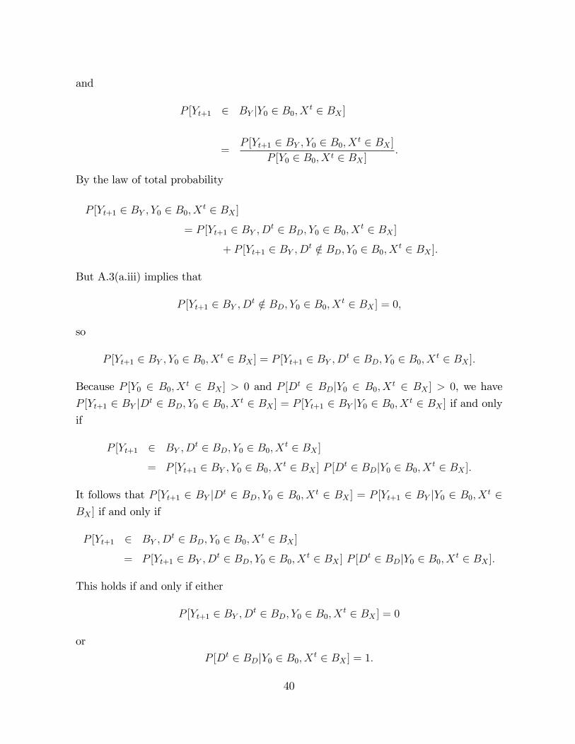
and

P [Yt+1 2 BY jY0 2 B0; X t 2 BX ]

=P [Yt+1 2 BY ; Y0 2 B0; X t 2 BX ]

P [Y0 2 B0; X t 2 BX ]:

By the law of total probability

P [Yt+1 2 BY ; Y0 2 B0; X t 2 BX ]= P [Yt+1 2 BY ; Dt 2 BD; Y0 2 B0; X t 2 BX ]

+ P [Yt+1 2 BY ; Dt =2 BD; Y0 2 B0; X t 2 BX ]:

But A.3(a.iii) implies that

P [Yt+1 2 BY ; Dt =2 BD; Y0 2 B0; X t 2 BX ] = 0;

so

P [Yt+1 2 BY ; Y0 2 B0; X t 2 BX ] = P [Yt+1 2 BY ; Dt 2 BD; Y0 2 B0; X t 2 BX ]:

Because P [Y0 2 B0; Xt 2 BX ] > 0 and P [Dt 2 BDjY0 2 B0; X

t 2 BX ] > 0, we have

P [Yt+1 2 BY jDt 2 BD; Y0 2 B0; X t 2 BX ] = P [Yt+1 2 BY jY0 2 B0; X t 2 BX ] if and onlyif

P [Yt+1 2 BY ; Dt 2 BD; Y0 2 B0; X t 2 BX ]

= P [Yt+1 2 BY ; Y0 2 B0; X t 2 BX ] P [Dt 2 BDjY0 2 B0; X t 2 BX ]:

It follows that P [Yt+1 2 BY jDt 2 BD; Y0 2 B0; Xt 2 BX ] = P [Yt+1 2 BY jY0 2 B0; X

t 2BX ] if and only if

P [Yt+1 2 BY ; Dt 2 BD; Y0 2 B0; X t 2 BX ]

= P [Yt+1 2 BY ; Dt 2 BD; Y0 2 B0; X t 2 BX ] P [Dt 2 BDjY0 2 B0; X t 2 BX ]:

This holds if and only if either

P [Yt+1 2 BY ; Dt 2 BD; Y0 2 B0; X t 2 BX ] = 0

or

P [Dt 2 BDjY0 2 B0; X t 2 BX ] = 1:

40

But these possibilities are ruled out by A.3(a.i) and A.3(a.ii) respectively. It follows that

P [Yt+1 2 BY jDt 2 BD; Y0 2 B0; X t 2 BX ]6= P [Yt+1 2 BY jY0 2 B0; X t 2 BX ];

and the proof of part (a) is complete. The proof of part (b) is similar. �

Proof of Proposition 4.1: For part (a), using the same argument as in Proposition 4.3of White and Kennedy (2008), we obtain




t = 1; ::: .

Then by applying A.5, we have




t = 1; ::: .

The proof of part (b) exactly follows Proposition 4.3 of White and Kennedy (2008). �

Proof of Proposition 4.2: For part(a), �rst we show necessity. Suppose Yt+1 ? Dt jYt; X

tt�� for all t = 0; 1::: : Take t = 0: Then by Proposition 4.1(a), we have

dF1;0(y1jy0; d0; x0) = dF�� (y1jy0; d0; x0�� )= dF�� (y1jy0; x0�� );

where the second equation follows from the maintained hypothesis. We also have for

t = 1; :::

dF� (yt+1jyt; dt; xtt�� ) = dF�� (yt+1jyt; xtt�� ):

By the maintained hypothesis, the recursions of Proposition 4.1(a) give


ZdF�� (yt+1jyt; dt; xtt�� )dFt;t�1(ytjy0; dt�1; xt�1)

=

ZdF�� (yt+1jyt; xtt�� )dFt;t�1(ytjy0; xt�1);

= dFt+1;t(yt+1jy0; xt)

41

t = 1; ::: .

so that necessity is proved.

For su¢ ciency, we give a proof by contradiction. Suppose there exists some t0 such

that Yt0+1 6? Dt0jYt0 ; X t0t0�� : This ensures that dF�� (yt0+1jyt0 ; dt0 ; x

t0t0�� ) must be a non-

constant function of dt0 on a set of positive probability. It follows that dF�� (y1jy0; d0; x0�� )must be a non-constant function of d0 on a set of positive probability, since we assume

the conditional density dF�� is the same for all t: By Proposition 4.1(a) for t = 0, we have

dF1;0(y1jy0; d0; x0) = dF�� (y1jy0; d0; x0�� ):

This implies that dF1;0(y1jy0; d0; x0) is a non-constant function of d0 on a set of positiveprobability. But this contradicts Yt+1 ? Dt j Y0; X t when t = 0: The su¢ ciency part is

proved and the proof of part (a) is complete. The proof of part (b) is similar. �

Proof of Proposition 5.1: For part (a), A.6(a.ii), i.e., Dt ? ( �U t; ~W0) j Y0; U t; X t; and

Dt ? U t j Y0; X t imply

(U t; �U t; ~W0) ? Dt j Y0; X t (A.i)

by D Lemma 4.3. (U t; �U t; ~W0) ? Dt j Y0; X t implies (U t; �U t; ~W0; Xt) ? Dt j Y0; X t by

D Lemma 4.1. Since ~Wt+1 = b3;t+1( ~Wt; X t; U t; �U t); by recursive substitution, there exists

some measurable function ft+1 such that ~Wt+1 = ft+1( ~W0; Xt; U t; �U t): Hence (U t; �U t; ~W0;

X t) ? Dt j Y0; X t implies ( ~Wt+1; ~W0) ? Dt j Y0; X t by D Lemma 4.2(i). ( ~Wt+1; ~W0) ?Dt j Y0; X t implies ~Wt+1 ? Dt j ~W0; Y0; X

t by D Lemma 4.2(ii). Further, A.7(a) implies~Wt+1 ? Y0 j ~W0; X

t by D Lemma 4.2. ~Wt+1 ? Y0 j ~W0; Xt and ~Wt+1 ? Dt j ~W0; Y0; X

t

together imply ~Wt+1 ? Dt j ~W0; Xt by D Lemma 4.3. The proof of part(a) is complete.

The proof of part(b) is parallel, replacing X t with XT : �

Proof of Proposition 5.2: For part (a), we �rst show that dFt+1;t( ~wt+1j ~w0; dt; xt) hasthe following recursive representation:

dF1;0( ~w1j ~w0; d0; x0) = dF�� ( ~w1j ~w0; d0; x0�� ) t = 0 (A.ii)

dFt+1;t( ~wt+1j ~w0; dt; xt) =ZdF�� ( ~wt+1j ~wt; dt; xtt�� ) dFt;t�1( ~wtj ~w0; dt�1; xt�1)

t = 1; ::: . (A.iii)

Eq.(A.ii) follows directly from A.8(a) when t = 0: Viewing ~Wt as a state vector, we have

the prediction density equation

dFt+1;t( ~wt+1j ~w0; dt; xt) =ZdFt+1;t( ~wt+1j ~wt; ~w0; dt; xt) dFt;t�1( ~wtj ~w0; dt; xt):

42

To verify eq.(A.iii), it su¢ ces to verify eqs.(A.iv), (A.v), and (A.vi):

dFt+1;t( ~wt+1j ~wt; ~w0; dt; xt) = dFt+1;t( ~wt+1j ~wt; dt; xt) (A.iv)

= dF�� ( ~wt+1j ~wt; dt; xtt�� ) (A.v)

dFt;t�1( ~wtj ~w0; dt; xt) = dFt;t�1( ~wtj ~w0; dt�1; xt�1): (A.vi)

Eq.(A.v) is A.6(a). Eq.(A.iv) says that ~Wt+1 ? ( ~W0;Dt�1) j ~Wt; Dt; X

t: We now

verify this. Now (U t; �U t; ~W0) ? Dt j Y0; X t (eq.(A.i)) implies (U t; �U t; ~W0; Xt) ? Dt j

~W0; Y0; Xt by D Lemma 4.1. Since ( ~Wt+1; ~Wt) is a function of ( ~W0; U

t; �U t; X t) by recursive

substitution, (U t; �U t; ~W0; Xt) ? Dt j ~W0; Y0; X

t implies ( ~Wt+1; ~Wt) ? Dt j ~W0; Y0; Xt by

D Lemma 4.2(i). ( ~Wt+1; ~Wt) ? Dt j ~W0; Y0; Xt implies ~Wt+1 ? Dt j ~W0; ~Wt; Y0; X

t

by D Lemma 4.2(ii). A.7(a) implies ~Wt+1 ? (Y0; ~W0) j ~Wt; Xt by D Lemma 4.2(ii).

~Wt+1 ? (Y0; ~W0) j ~Wt; Xt implies ~Wt+1 ? Y0 j ~W0; ~Wt; X

t by D Lemma 4.2(ii). ~Wt+1 ?Y0 j ~W0; ~Wt; X

t and ~Wt+1 ? Dt j ~W0; ~Wt; Y0; Xt imply ~Wt+1 ? Dt j ~W0; ~Wt; X

t by D

Lemma 4.3. A.7(a) also implies ~Wt+1 ? ~W0 j ~Wt; Xt by D Lemma 4.2. ~Wt+1 ? ~W0 j

~Wt; Xt and ~Wt+1 ? Dt j ~W0; ~Wt; X

t imply ~Wt+1 ? ( ~W0; Dt) j ~Wt; X

t by D Lemma 4.3.~Wt+1 ? ( ~W0; D

t) j ~Wt; Xt implies ~Wt+1 ? ( ~W0; D

t) j ~Wt; Dt; Xt by D Lemma 4.2(ii).

Further ~Wt+1 ? ( ~W0; Dt) j ~Wt; Dt; X

t implies ~Wt+1 ? ( ~W0; Dt�1) j ~Wt; Dt; X

t by D

Lemma 4.2(i). This veri�es eq.(A.iv).

Eq.(A.vi) says that ~Wt ? (Dt; Xt) j ~W0; Dt�1; X t�1: We now verify this. Now (U t; �U t;

~W0) ? Dt j Y0; X t (eq.(A.i)) implies (U t; �U t; ~W0) ? Dt j ~W0; Y0; Xt by D Lemma 4.2(ii).

(U t; �U t; ~W0) ? Dt j ~W0; Y0; Xt implies (U t; �U t; ~W0; X

t) ? Dt j ~W0; Y0; Xt by D Lemma

4.1. (U t; �U t; ~W0; Xt) ? Dt j ~W0; Y0; X

t implies ~Wt ? Dt j ~W0; Y0; Xt; since ~Wt is a

function of (U t; �U t; ~W0; Xt) by recursive substitution. A.7(a) implies ~Wt ? Y0 j ~W0; X

t

by D Lemma 4.2. ~Wt ? Y0 j ~W0; Xt and ~Wt ? Dt j ~W0; Y0; X

t imply ~Wt ? Dt j ~W0; Xt by

D Lemma 4.3. ~Wt ? Dt j ~W0; Xt and A.9 imply ~Wt ? (Dt; Xt) j ~W0; X

t�1 by D Lemma

4.3. ~Wt ? (Dt; Xt) j ~W0; Xt�1 implies ~Wt ? (Dt; Xt) j ~W0; D

t�1; X t�1 by D Lemma 4.2.

This veri�es eq.(A.vi).

With the recursive representation of dFt+1;t( ~wt+1j ~w0; dt; xt), the rest of the proof ofpart (a) follows the proof of Proposition 4.2(a) exactly. The proof of part (a) is thus

complete. The proof of part (b) is analogous. �

Proof of Proposition 5.3: We �rst de�ne the null hypothesis H0 and alternative hy-

pothesis HA. We denote (retrospective) conditional exogeneity H1 and (retrospective)

43

(weak) G non-causality H2: Then H0 and HA are de�ned as

H0 : Either H1 does not hold or H2 holds.

HA : H1 holds and H2 does not hold.

Under H0; we fail to reject structural non-causality. Under HA; we reject structural non-

causality. Let P0 denote the true probability measure under H0: There are three cases

under H0.

Case 1: H1 holds and H2 holds. In this case,

� = P0 [fail to reject H1 and reject H2]

� min fP0 [fail to reject H1 ] , P0 [reject H2]g= minf1� �1; �2g; and

� = 1� P0 [reject H1 or fail to reject H2]

� 1� P0 [reject H1]� P0 [fail to reject H2]

= 1� �1 � (1� �2) = �2 � �1:

Case 2: H1 does not hold and H2 does not hold. Similarly, in this case,

� � min fP0 [fail to reject H1] , P0 [reject H2]g= minf1� �1; �2g; and

� � 1� P0 [reject H1]� P0 [fail to reject H2]

= 1� �1 � (1� �2) = �2 � �1:

Case 3: H1 does not hold and H2 holds. Similarly, in this case,

� � min fP0 [fail to reject H1 ] , P0 [reject H2]g= minf1� �1; �2g; and

� � 1� P0 [reject H1]� P0 [fail to reject H2]

= 1� �1 � (1� �2) = �2 � �1:

Combining the three cases gives

� � maxfminf1� �1; �2g;minf1� �1; �2g;minf1� �1; �2gg and� � max f0;min f(�2 � �1) ; (�2 � �1) ; (�2 � �1)gg :

44

Let PA denote the probability measure under HA: Then

� = 1� PA [Either reject H1 or fail to reject H2]

� 1� PA [reject H1]� PA [fail to reject H2]

= 1� �1 � (1� �2) = �2 � �1; and

� = PA [fail to reject H1 and reject H2]

� min fPA [fail to reject H1] ; PA [reject H2]g= min f1� �1; �2g :

Hence,

�2 � �1 � � � min f1� �1; �2g : �

Proof of Proposition 5.4: FromProposition 5.3, we have �T � maxfminf1��1T ; �2Tg;minf1��1T ; �2Tg;minf1� �1T ; �2Tgg, which implies

lim sup�T � lim sup fmaxfminf1� �1T ; �2Tg;minf1� �1T ; �2Tg;minf1� �1T ; �2Tggg= lim fmaxfminf1� �1T ; �2Tg;minf1� �1T ; �2Tg;minf1� �1T ; �2Tggg= maxfmin f1� �1; �2g ;min f0; 1g ;min f0; �2gg = min f1� �1; �2g :

Also from Proposition 5.3, we have �T � fmax 0;min f(�2T � �1T ) ; (�2T � �1T ) ; (�2T � �1T )gg ;which implies

lim inf �T � lim inf fmax f0;min f(�2T � �1T ) ; (�2T � �1T ) ; (�2T � �1T )ggg= lim fmax f0;min f(�2T � �1T ) ; (�2T � �1T ) ; (�2T � �1T )ggg= maxf0;min f(�2 � �1) ; 0; (�2 � 1)gg = 0:

Thus,

0 � lim inf �T � lim sup�T � min f1� �1; �2g :

From Proposition 5.3, we have �T � min f1� �1T ; �2Tg, which implies

lim sup�T � lim sup fmin f1� �1T ; �2Tgg= lim fmin f1� �1T ; �2Tgg= minf1� �1; 1g = 1� �1:

Also from Proposition 5.3, we have �T � �2T � �1T , which implies

lim inf �T � lim inf (�2T � �1T )

= lim (�2T � �1T )

= 1� �1:

45

Thus,

1� �1 � lim inf �T � lim sup�T � 1� �1:

This further implies

lim �T = 1� �1: �

References

[1] Angrist, J. and G. Kuersteiner (2004), "Semiparametric Causality Tests Using the

Policy Propensity Score," NBER Working Paper No. 10975.

[2] Borenstein, S., A. Cameron, and R. Gilbert (1997), "Do Gasoline Prices Respond

Asymmetrically to Crude Oil Price Changes," Quarterly Journal of Economics, 112,

305-339.

[3] Candès, E. (1999), "Ridgelets: Estimating with Ridge Functions," Annals of Statis-

tics, 31, 1561-1599.

[4] Chalak, K. and H. White (2007a), "Independence and Conditional Independence in

Causal Systems," UCSD Dept. of Economics Discussion Paper.

[5] Chalak, K. and H. White (2007b), "Identi�cation with Conditioning Instruments in

Causal Systems," UCSD Dept. of Economics Discussion Paper.

[6] Chalak, K. and H. White (2007c), "An Extended Class of Instrumental Variables for

the Estimation of Causal E¤ects," UCSD Dept. of Economics Discussion Paper.

[7] Chen, N., R. Roll and S. Ross (1986), "Economic Forces and the Stock Market,"

Journal of Business, 59, 383-403.

[8] Chow, G. (1997). Dynamic Economics: Optimization by the Lagrange Method. Ox-

ford: Oxford University Press.

[9] Dawid, A.P. (1979), "Conditional Independence in Statistical Theory," Journal of

the Royal Statistical Society, Series B, 41, 1-31.

[10] Delgado, M. A. and W. Gonzalez-Manteiga (2001), "Signi�cance Testing in Nonpara-

metric Regression Based on the Bootstrap," Annals of Statistics, 29, 1469-1507.

46

[11] Fernandes, M. and R. G. Flores (2001), "Tests for Conditional Independence,

Markovian Dynamics, and Noncausality," Discussion Paper, European University

Institute.

[12] Fisher, F. (1966). The Identi�cation Problem in Econometrics. New York: McGraw-

Hill.

[13] Fisher, F. (1970), "A Correspondence Principle for Simultaneous Equations Models,"

Econometrica, 38, 73-92.

[14] Flannery, M. and A. Protopapadakis, 2002, "Macroeconomic Factors Do In�uence

Aggregate Stock Returns," Review of Financial Studies, 15, 751�782.

[15] Florens, J.P. and D. Fougère (1996), "Non-causality in Continuous Time," Econo-

metrica, 64, 1195�1212.

[16] Florens, J.P. and M. Mouchart (1982), "A Note on Non-causality," Econometrica,

50, 583�591.

[17] Goldberger, A. (1972), "Structural Equation Methods in the Social Sciences," Econo-

metrica, 40, 979-1001.

[18] Granger, C.W.J. (1969), "Investigating Causal Relations by Econometric Models and

Cross-spectral Methods," Econometrica, 37, 424�438.

[19] Granger, C.W.J. (1980), "Testing for Causality, a Personal Viewpoint," Journal of

Economic Dynamics and Control, 2, 329-352.

[20] Granger, C.W.J. (1988), "Some Recent Developments in a Concept of Causality,"

Journal of Econometrics, 39, 199-211.

[21] Granger, C.W.J. and P. Newbold (1986). Forecasting Economic Time Series. New

York: Academic Press (2nd edition).

[22] Heckman, J. (2008), "Econometric Causality," NBER Working Paper No. 13934.

[23] Hochberg, Y. (1988), "A Sharper Bonferroni Procedure for Multiple Tests of Signi�-

cance," Biometrika, 75, 800�802.

[24] Leeper, E. (1997), "Narrative and VAR approaches to Monetary Policy: Common

Identi�cation Problems," Journal of Monetary Economics, 40, 641-657.

47

[25] Linton, O. and P. Gozalo (1997), "Conditional Independence Restrictions: Testing

and Estimation," Discussion Paper, Cowles Foundation for Research in Economics,

Yale University.

[26] Newey, W. K. and K. D.West (1987), "A Simple, Positive Semide�nite, Heteroskedas-

ticity and Autocorrelation Consistent Covariance Matrix," Econometrica, 55, 703-

708.

[27] Reichenbach, H. (1956). The Direction of Time. Berkeley: University of California

Press.

[28] Romer, C. and D. Romer (1989), "Does Monetary Policy Matter? A New Test in

the Spirit of Friedman and Schwartz," NBER Macroeconomics Annual, 4, 121-170.

[29] Romer, C. and D. Romer (1994), "Monetary Policy Matters," Journal of Monetary

Economics, 34, 75-88.

[30] Shapiro, M. (1994), "Federal Reserve Policy: Cause and E¤ect," in G. Mankiw, ed.,

Monetary Policy. Chicago: University of Chicago Press, 307-334.

[31] Sims, C. (1972), "Money, Income, and Causality," American Economic Review, 62,

540-552.

[32] Strotz, R. and H. Wold (1960), "Recursive vs. Nonrecursive Systems: An Attempt

at Synthesis," Econometrica, 28, 417-427.

[33] Su, L. and H. White (2007a), "A Consistent Characteristic Function-Based Test for

Conditional Independence," Journal of Econometrics, 141, 807-834.

[34] Su, L. and H. White (2007b), "Testing Conditional Independence via Empirical Like-

lihood," UCSD Dept. of Economics Discussion Paper.

[35] Su, L. and H. White (2008), "A Nonparametric Hellinger Metric Test for Conditional

Independence," Econometric Theory, 24, 829�864.

[36] White, H. (2006a), "Time-series Estimation of the E¤ects of Natural Experiments,"

Journal of Econometrics, 135, 527-566.

[37] White, H (2006b), "Approximate Nonlinear Forecasting Methods," in G. Elliott,

C.W.J. Granger, and A. Timmermann, eds., Handbook of Economic Forecasting.

New York: Elsevier, 460-512.

48

[38] White, H. and K. Chalak (2007a), "Identifying E¤ects of Endogenous Causes in Non-

separable Systems Using Covariates," UCSD Dept. of Economics Discussion Paper.

[39] White, H. and K. Chalak (2007b), "Settable Systems: An Extension of Pearl�s Causal

Model with Optimization, Equilibrium, and Learning," UCSD Dept. of Economics

Discussion Paper.

[40] White, H. and K. Chalak (2007c), "Parametric and Nonparametric Estimation of

Covariate-Conditioned Average E¤ects," UCSD Dept. of Economics Discussion Pa-

per.

[41] White, H. and P. Kennedy (2008), "Retrospective Estimation of Causal E¤ects

Through Time," in J. Castle and N. Shephard, eds., A Festschrift in Honour of

David Hendry. Oxford: Oxford University Press (forthcoming).

49

Granger Causality and Dynamic Structural Systemswebfac/bgraham/secnf/white.pdfKarim Chalak, and...

Documents

Transcript of Granger Causality and Dynamic Structural Systemswebfac/bgraham/secnf/white.pdfKarim Chalak, and...