ANNIVERSARY REVIEW

Grain boundary energy anisotropy: a review

Gregory S. Rohrer

Received: 29 April 2011 / Accepted: 30 May 2011 / Published online: 10 June 2011! Springer Science+Business Media, LLC 2011

Abstract This paper reviews findings on the anisotropyof the grain boundary energies. After introducing the basic

concepts, there is a discussion of fundamental models used

to understand and predict grain boundary energy anisot-ropy. Experimental methods for measuring the grain

boundary energy anisotropy, all of which involve appli-

cation of the Herring equation, are then briefly described.The next section reviews and compares the results of

measurements and model calculations with the goal of

identifying generally applicable characteristics. This isfollowed by a brief discussion of the role of grain boundary

energies in nucleating discontinuous transitions in grain

boundary structure and chemistry, known as complexiontransitions. The review ends with some questions to be

addressed by future research and a summary of what is

known about grain boundary energy anisotropy.

Introduction

The vast majority of the solid materials used in engineered

systems are polycrystalline. In other words, they arecomprised of many single crystals joined together by a

three-dimensional (3D) network of internal interfaces

called grain boundaries. Because the performance andintegrity of a material are often determined by the structure

of this network, grain boundaries have been of interest to

materials scientists for many decades. There have beenseveral recent review articles surveying grain boundary

phenomena [1–5]. The current review is more narrowly

focused on the topic of grain boundary energy anisotropyand provides an account of advancements since the publi-

cation of Sutton and Balluffi’s [6] critical review of grain

boundary energy data in 1987. The paper contains a briefsurvey of historical concepts and grain boundary energy

measurements. Next, findings from experiments and sim-

ulations are reviewed. This is followed by an introductionto recent findings about complexion transitions at grain

boundaries. The review concludes with a prospectus for

future studies of grain boundary energy anisotropy and asummary.

Grain boundaries are defects that have an excess free

energy per unit area. This is evident by the fact that duringmost thermal and chemical etching processes, material near

the grain boundary is preferentially removed. If a solid

surface is polished and then etched, the preferentialremoval of material near the grain boundaries reveals the

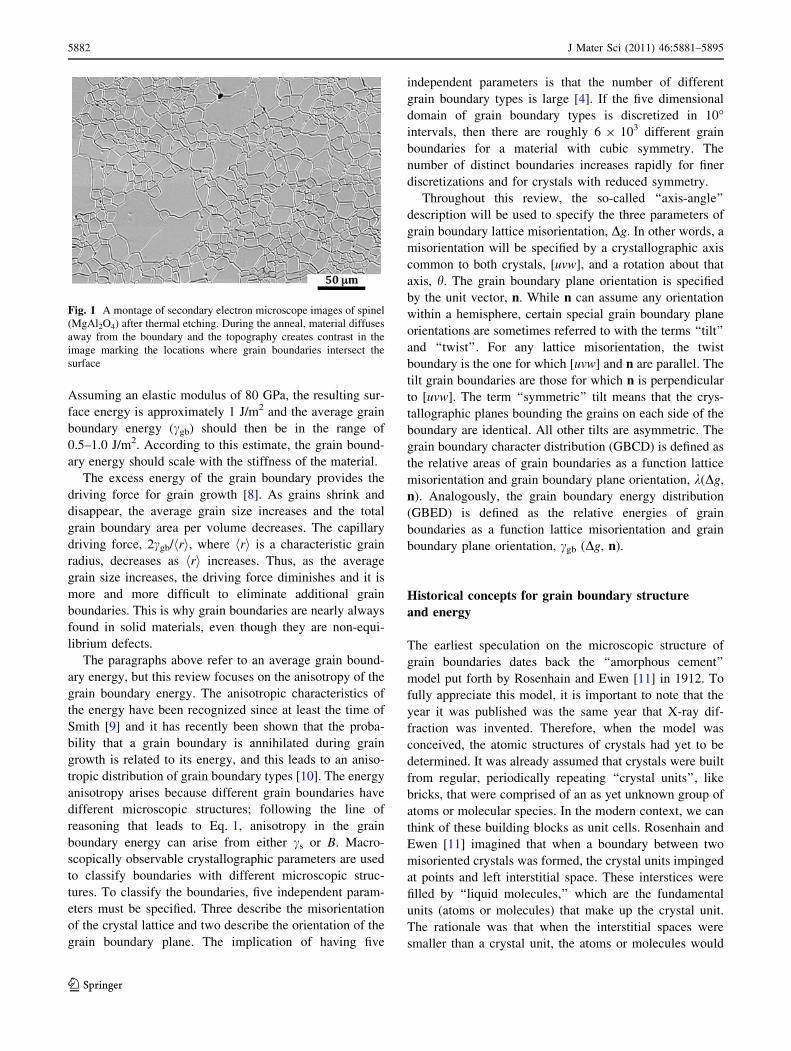
interfacial network, as illustrated in Fig. 1. To make a

rough estimate for the average excess energy of a grainboundary, we can imagine building the interface by first

creating two free surfaces and then joining them together toform the boundary. The energy to create the two surfaces

will be twice the surface energy, 2cs. However, the grain

boundary energy will be less than this because of thebinding energy (B) gained when the two surfaces are

brought together and new bonds are formed. The grain

boundary energy is then:

cgb ! 2cs " B #1$

If we guess that the bonding at the interface restores

one-half to three-quarters of the bonds to each side, thencs/2 B B B 3cs/4 and cs/2 B cgb\ cs. Using some simple

approximations, Mullins [7] estimated cs as the elastic

work done to create a free surface and found it to be(E/8) 9 10-10 m, where E is the elastic modulus.

G. S. Rohrer (&)Department of Materials Science and Engineering, CarnegieMellon University, Pittsburgh, PA 15213-3890, USAe-mail: rohrer@cmu.edu

123

J Mater Sci (2011) 46:5881–5895

DOI 10.1007/s10853-011-5677-3

Assuming an elastic modulus of 80 GPa, the resulting sur-face energy is approximately 1 J/m2 and the average grain

boundary energy (cgb) should then be in the range of

0.5–1.0 J/m2. According to this estimate, the grain bound-ary energy should scale with the stiffness of the material.

The excess energy of the grain boundary provides the

driving force for grain growth [8]. As grains shrink anddisappear, the average grain size increases and the total

grain boundary area per volume decreases. The capillary

driving force, 2cgb/hri, where hri is a characteristic grainradius, decreases as hri increases. Thus, as the average

grain size increases, the driving force diminishes and it is

more and more difficult to eliminate additional grainboundaries. This is why grain boundaries are nearly always

found in solid materials, even though they are non-equi-

librium defects.The paragraphs above refer to an average grain bound-

ary energy, but this review focuses on the anisotropy of the

grain boundary energy. The anisotropic characteristics ofthe energy have been recognized since at least the time of

Smith [9] and it has recently been shown that the proba-

bility that a grain boundary is annihilated during graingrowth is related to its energy, and this leads to an aniso-

tropic distribution of grain boundary types [10]. The energy

anisotropy arises because different grain boundaries havedifferent microscopic structures; following the line of

reasoning that leads to Eq. 1, anisotropy in the grain

boundary energy can arise from either cs or B. Macro-scopically observable crystallographic parameters are used

to classify boundaries with different microscopic struc-

tures. To classify the boundaries, five independent param-eters must be specified. Three describe the misorientation

of the crystal lattice and two describe the orientation of the

grain boundary plane. The implication of having five

independent parameters is that the number of different

grain boundary types is large [4]. If the five dimensionaldomain of grain boundary types is discretized in 10"intervals, then there are roughly 6 9 103 different grain

boundaries for a material with cubic symmetry. Thenumber of distinct boundaries increases rapidly for finer

discretizations and for crystals with reduced symmetry.

Throughout this review, the so-called ‘‘axis-angle’’description will be used to specify the three parameters of

grain boundary lattice misorientation, Dg. In other words, amisorientation will be specified by a crystallographic axis

common to both crystals, [uvw], and a rotation about that

axis, h. The grain boundary plane orientation is specifiedby the unit vector, n. While n can assume any orientation

within a hemisphere, certain special grain boundary plane

orientations are sometimes referred to with the terms ‘‘tilt’’and ‘‘twist’’. For any lattice misorientation, the twist

boundary is the one for which [uvw] and n are parallel. The

tilt grain boundaries are those for which n is perpendicularto [uvw]. The term ‘‘symmetric’’ tilt means that the crys-

tallographic planes bounding the grains on each side of the

boundary are identical. All other tilts are asymmetric. Thegrain boundary character distribution (GBCD) is defined as

the relative areas of grain boundaries as a function lattice

misorientation and grain boundary plane orientation, k(Dg,n). Analogously, the grain boundary energy distribution

(GBED) is defined as the relative energies of grain

boundaries as a function lattice misorientation and grainboundary plane orientation, cgb (Dg, n).

Historical concepts for grain boundary structureand energy

The earliest speculation on the microscopic structure of

grain boundaries dates back the ‘‘amorphous cement’’

model put forth by Rosenhain and Ewen [11] in 1912. Tofully appreciate this model, it is important to note that the

year it was published was the same year that X-ray dif-

fraction was invented. Therefore, when the model wasconceived, the atomic structures of crystals had yet to be

determined. It was already assumed that crystals were built

from regular, periodically repeating ‘‘crystal units’’, likebricks, that were comprised of an as yet unknown group of

atoms or molecular species. In the modern context, we can

think of these building blocks as unit cells. Rosenhain andEwen [11] imagined that when a boundary between two

misoriented crystals was formed, the crystal units impinged

at points and left interstitial space. These interstices werefilled by ‘‘liquid molecules,’’ which are the fundamental

units (atoms or molecules) that make up the crystal unit.

The rationale was that when the interstitial spaces weresmaller than a crystal unit, the atoms or molecules would

Fig. 1 A montage of secondary electron microscope images of spinel(MgAl2O4) after thermal etching. During the anneal, material diffusesaway from the boundary and the topography creates contrast in theimage marking the locations where grain boundaries intersect thesurface

5882 J Mater Sci (2011) 46:5881–5895

123

be unable to aggregate and, not crystallizing, would remain

amorphous. The uncrystallized material was referred to asan ‘‘amorphous cement’’ that held the boundary together.

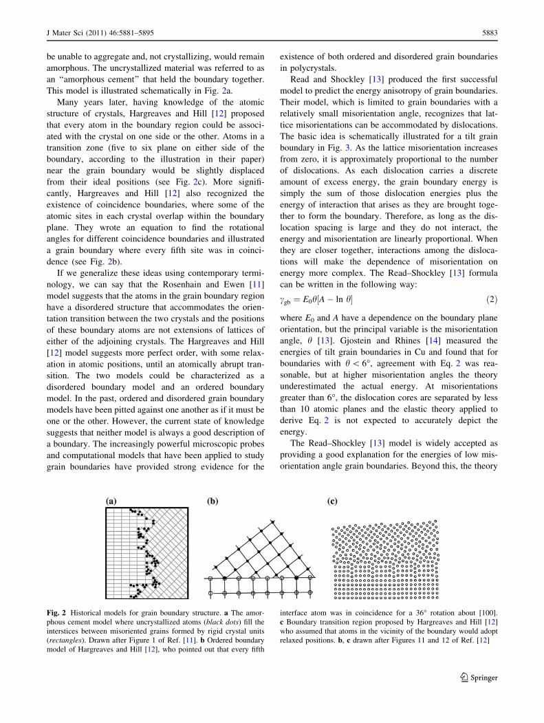
This model is illustrated schematically in Fig. 2a.

Many years later, having knowledge of the atomicstructure of crystals, Hargreaves and Hill [12] proposed

that every atom in the boundary region could be associ-

ated with the crystal on one side or the other. Atoms in atransition zone (five to six plane on either side of the

boundary, according to the illustration in their paper)near the grain boundary would be slightly displaced

from their ideal positions (see Fig. 2c). More signifi-

cantly, Hargreaves and Hill [12] also recognized theexistence of coincidence boundaries, where some of the

atomic sites in each crystal overlap within the boundary

plane. They wrote an equation to find the rotationalangles for different coincidence boundaries and illustrated

a grain boundary where every fifth site was in coinci-

dence (see Fig. 2b).If we generalize these ideas using contemporary termi-

nology, we can say that the Rosenhain and Ewen [11]

model suggests that the atoms in the grain boundary regionhave a disordered structure that accommodates the orien-

tation transition between the two crystals and the positions

of these boundary atoms are not extensions of lattices ofeither of the adjoining crystals. The Hargreaves and Hill

[12] model suggests more perfect order, with some relax-

ation in atomic positions, until an atomically abrupt tran-sition. The two models could be characterized as a

disordered boundary model and an ordered boundary

model. In the past, ordered and disordered grain boundarymodels have been pitted against one another as if it must be

one or the other. However, the current state of knowledge

suggests that neither model is always a good description ofa boundary. The increasingly powerful microscopic probes

and computational models that have been applied to study

grain boundaries have provided strong evidence for the

existence of both ordered and disordered grain boundaries

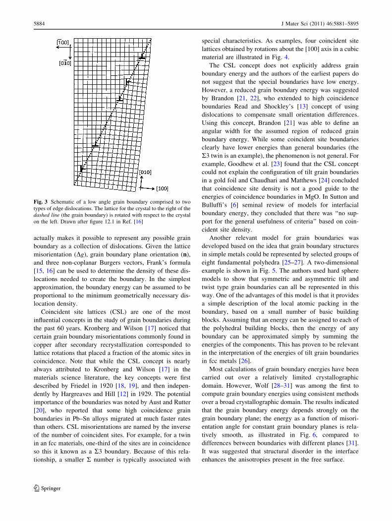
in polycrystals.Read and Shockley [13] produced the first successful

model to predict the energy anisotropy of grain boundaries.

Their model, which is limited to grain boundaries with arelatively small misorientation angle, recognizes that lat-

tice misorientations can be accommodated by dislocations.

The basic idea is schematically illustrated for a tilt grainboundary in Fig. 3. As the lattice misorientation increases

from zero, it is approximately proportional to the numberof dislocations. As each dislocation carries a discrete

amount of excess energy, the grain boundary energy is

simply the sum of those dislocation energies plus theenergy of interaction that arises as they are brought toge-

ther to form the boundary. Therefore, as long as the dis-

location spacing is large and they do not interact, theenergy and misorientation are linearly proportional. When

they are closer together, interactions among the disloca-

tions will make the dependence of misorientation onenergy more complex. The Read–Shockley [13] formula

can be written in the following way:

cgb ! E0h%A" ln h& #2$

where E0 and A have a dependence on the boundary plane

orientation, but the principal variable is the misorientation

angle, h [13]. Gjostein and Rhines [14] measured theenergies of tilt grain boundaries in Cu and found that for

boundaries with h\ 6", agreement with Eq. 2 was rea-

sonable, but at higher misorientation angles the theoryunderestimated the actual energy. At misorientations

greater than 6", the dislocation cores are separated by less

than 10 atomic planes and the elastic theory applied toderive Eq. 2 is not expected to accurately depict the

energy.

The Read–Shockley [13] model is widely accepted asproviding a good explanation for the energies of low mis-

orientation angle grain boundaries. Beyond this, the theory

Fig. 2 Historical models for grain boundary structure. a The amor-phous cement model where uncrystallized atoms (black dots) fill theinterstices between misoriented grains formed by rigid crystal units(rectangles). Drawn after Figure 1 of Ref. [11]. b Ordered boundarymodel of Hargreaves and Hill [12], who pointed out that every fifth

interface atom was in coincidence for a 36" rotation about [100].c Boundary transition region proposed by Hargreaves and Hill [12]who assumed that atoms in the vicinity of the boundary would adoptrelaxed positions. b, c drawn after Figures 11 and 12 of Ref. [12]

J Mater Sci (2011) 46:5881–5895 5883

123

actually makes it possible to represent any possible grain

boundary as a collection of dislocations. Given the lattice

misorientation (Dg), grain boundary plane orientation (n),and three non-coplanar Burgers vectors, Frank’s formula

[15, 16] can be used to determine the density of these dis-

locations needed to create the boundary. In the simplestapproximation, the boundary energy can be assumed to be

proportional to the minimum geometrically necessary dis-location density.

Coincident site lattices (CSL) are one of the most

influential concepts in the study of grain boundaries duringthe past 60 years. Kronberg and Wilson [17] noticed that

certain grain boundary misorientations commonly found in

copper after secondary recrystallization corresponded tolattice rotations that placed a fraction of the atomic sites in

coincidence. Note that while the CSL concept is nearly

always attributed to Kronberg and Wilson [17] in thematerials science literature, the key concepts were first

described by Friedel in 1920 [18, 19], and then indepen-

dently by Hargreaves and Hill [12] in 1929. The potentialimportance of the boundaries was noted by Aust and Rutter

[20], who reported that some high coincidence grain

boundaries in Pb–Sn alloys migrated at much faster ratesthan others. CSL misorientations are named by the inverse

of the number of coincident sites. For example, for a twin

in an fcc materials, one-third of the sites are in coincidenceso this it known as a R3 boundary. Because of this rela-

tionship, a smaller R number is typically associated with

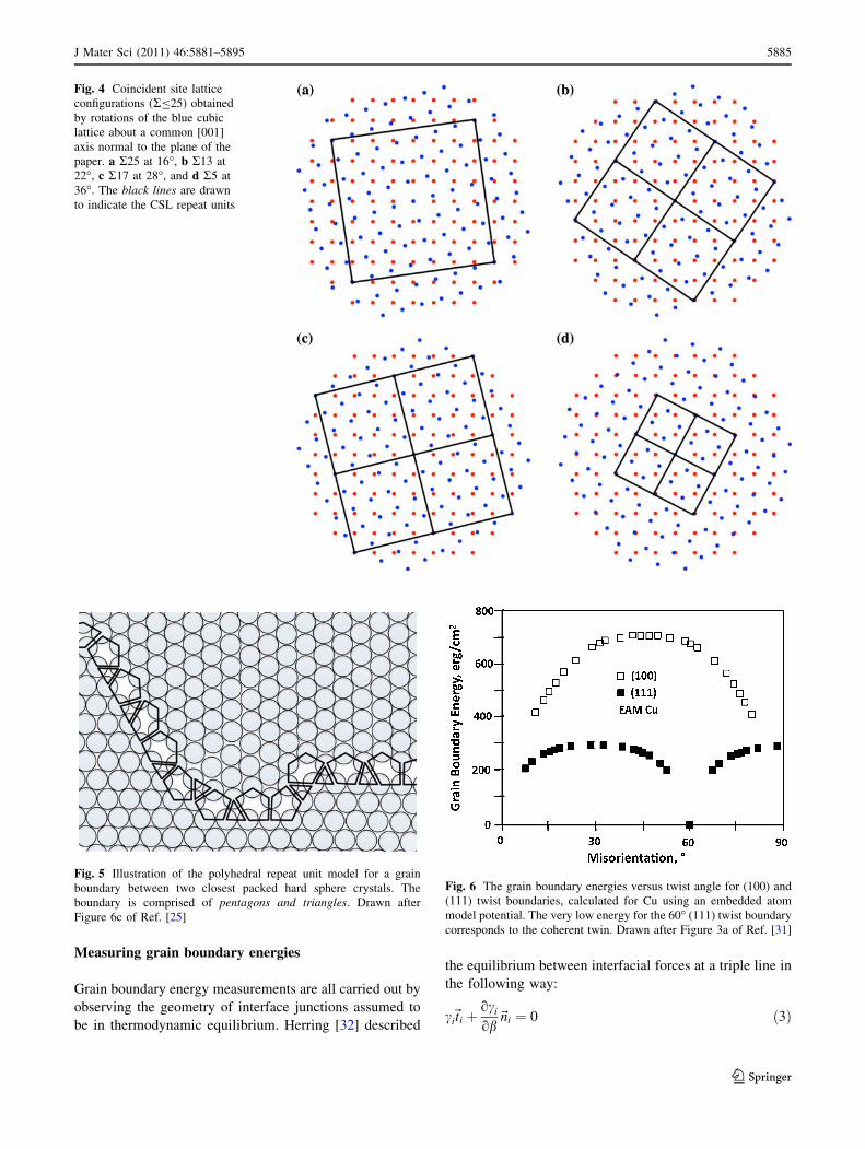
special characteristics. As examples, four coincident site

lattices obtained by rotations about the [100] axis in a cubicmaterial are illustrated in Fig. 4.

The CSL concept does not explicitly address grain

boundary energy and the authors of the earliest papers donot suggest that the special boundaries have low energy.

However, a reduced grain boundary energy was suggested

by Brandon [21, 22], who extended to high coincidenceboundaries Read and Shockley’s [13] concept of using

dislocations to compensate small orientation differences.Using this concept, Brandon [21] was able to define an

angular width for the assumed region of reduced grain

boundary energy. While some coincident site boundariesclearly have lower energies than general boundaries (the

R3 twin is an example), the phenomenon is not general. For

example, Goodhew et al. [23] found that the CSL conceptcould not explain the configuration of tilt grain boundaries

in a gold foil and Chaudhari and Matthews [24] concluded

that coincidence site density is not a good guide to theenergies of coincidence boundaries in MgO. In Sutton and

Bulluffi’s [6] seminal review of models for interfacial

boundary energy, they concluded that there was ‘‘no sup-port for the general usefulness of criteria’’ based on coin-

cident site density.

Another relevant model for grain boundaries wasdeveloped based on the idea that grain boundary structures

in simple metals could be represented by selected groups of

eight fundamental polyhedra [25–27]. A two-dimensionalexample is shown in Fig. 5. The authors used hard sphere

models to show that symmetric and asymmetric tilt and

twist type grain boundaries can all be represented in thisway. One of the advantages of this model is that it provides

a simple description of the local atomic packing in the

boundary, based on a small number of basic buildingblocks. Assuming that an energy can be assigned to each of

the polyhedral building blocks, then the energy of any

boundary can be approximated simply by summing theenergies of the components. This has proven to be relevant

in the interpretation of the energies of tilt grain boundaries

in fcc metals [26].Most calculations of grain boundary energies have been

carried out over a relatively limited crystallographic

domain. However, Wolf [28–31] was among the first tocompute grain boundary energies using consistent methods

over a broad crystallographic domain. The results indicated

that the grain boundary energy depends strongly on thegrain boundary plane; the energy as a function of misori-

entation angle for constant grain boundary planes is rela-

tively smooth, as illustrated in Fig. 6, compared todifferences between boundaries with different planes [31].

It was suggested that structural disorder in the interface

enhances the anisotropies present in the free surface.

Fig. 3 Schematic of a low angle grain boundary comprised to twotypes of edge dislocations. The lattice for the crystal to the right of thedashed line (the grain boundary) is rotated with respect to the crystalon the left. Drawn after figure 12.1 in Ref. [16]

5884 J Mater Sci (2011) 46:5881–5895

123

Measuring grain boundary energies

Grain boundary energy measurements are all carried out byobserving the geometry of interface junctions assumed to

be in thermodynamic equilibrium. Herring [32] described

the equilibrium between interfacial forces at a triple line in

the following way:

cit~i 'ociob

n~i ! 0 #3$

Fig. 4 Coincident site latticeconfigurations (RB25) obtainedby rotations of the blue cubiclattice about a common [001]axis normal to the plane of thepaper. a R25 at 16", b R13 at22", c R17 at 28", and d R5 at36". The black lines are drawnto indicate the CSL repeat units

Fig. 5 Illustration of the polyhedral repeat unit model for a grainboundary between two closest packed hard sphere crystals. Theboundary is comprised of pentagons and triangles. Drawn afterFigure 6c of Ref. [25]

Fig. 6 The grain boundary energies versus twist angle for (100) and(111) twist boundaries, calculated for Cu using an embedded atommodel potential. The very low energy for the 60" (111) twist boundarycorresponds to the coherent twin. Drawn after Figure 3a of Ref. [31]

J Mater Sci (2011) 46:5881–5895 5885

123

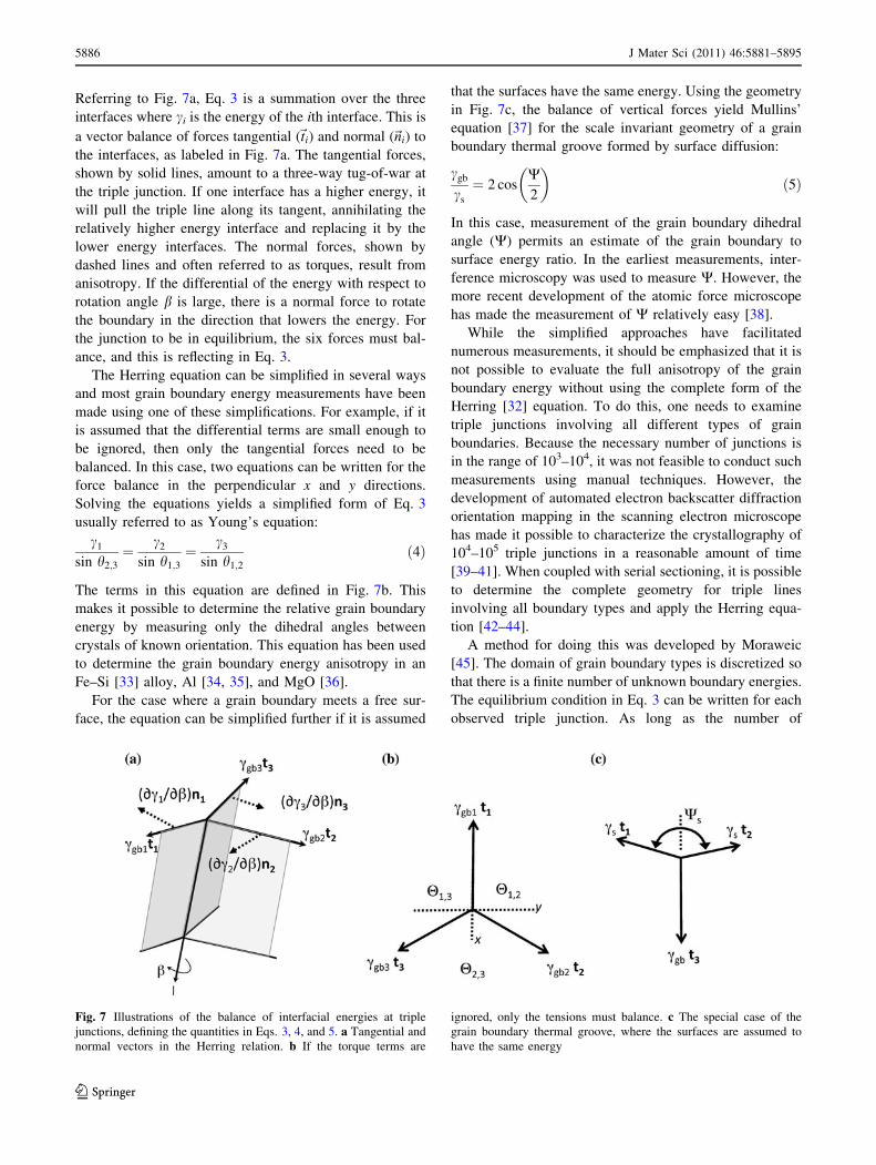
Referring to Fig. 7a, Eq. 3 is a summation over the three

interfaces where ci is the energy of the ith interface. This is

a vector balance of forces tangential (t~i) and normal (n~i) to

the interfaces, as labeled in Fig. 7a. The tangential forces,shown by solid lines, amount to a three-way tug-of-war at

the triple junction. If one interface has a higher energy, it

will pull the triple line along its tangent, annihilating therelatively higher energy interface and replacing it by the

lower energy interfaces. The normal forces, shown by

dashed lines and often referred to as torques, result fromanisotropy. If the differential of the energy with respect to

rotation angle b is large, there is a normal force to rotate

the boundary in the direction that lowers the energy. Forthe junction to be in equilibrium, the six forces must bal-

ance, and this is reflecting in Eq. 3.

The Herring equation can be simplified in several waysand most grain boundary energy measurements have been

made using one of these simplifications. For example, if itis assumed that the differential terms are small enough to

be ignored, then only the tangential forces need to be

balanced. In this case, two equations can be written for theforce balance in the perpendicular x and y directions.

Solving the equations yields a simplified form of Eq. 3

usually referred to as Young’s equation:

c1sin h2;3

! c2sin h1;3

! c3sin h1;2

#4$

The terms in this equation are defined in Fig. 7b. Thismakes it possible to determine the relative grain boundary

energy by measuring only the dihedral angles between

crystals of known orientation. This equation has been usedto determine the grain boundary energy anisotropy in an

Fe–Si [33] alloy, Al [34, 35], and MgO [36].

For the case where a grain boundary meets a free sur-face, the equation can be simplified further if it is assumed

that the surfaces have the same energy. Using the geometry

in Fig. 7c, the balance of vertical forces yield Mullins’equation [37] for the scale invariant geometry of a grain

boundary thermal groove formed by surface diffusion:

cgbcs

! 2 cosW2

! "#5$

In this case, measurement of the grain boundary dihedralangle (W) permits an estimate of the grain boundary to

surface energy ratio. In the earliest measurements, inter-

ference microscopy was used to measure W. However, themore recent development of the atomic force microscope

has made the measurement of W relatively easy [38].

While the simplified approaches have facilitatednumerous measurements, it should be emphasized that it is

not possible to evaluate the full anisotropy of the grain

boundary energy without using the complete form of theHerring [32] equation. To do this, one needs to examine

triple junctions involving all different types of grain

boundaries. Because the necessary number of junctions isin the range of 103–104, it was not feasible to conduct such

measurements using manual techniques. However, the

development of automated electron backscatter diffractionorientation mapping in the scanning electron microscope

has made it possible to characterize the crystallography of

104–105 triple junctions in a reasonable amount of time[39–41]. When coupled with serial sectioning, it is possible

to determine the complete geometry for triple lines

involving all boundary types and apply the Herring equa-tion [42–44].

A method for doing this was developed by Moraweic

[45]. The domain of grain boundary types is discretized sothat there is a finite number of unknown boundary energies.

The equilibrium condition in Eq. 3 can be written for each

observed triple junction. As long as the number of

Fig. 7 Illustrations of the balance of interfacial energies at triplejunctions, defining the quantities in Eqs. 3, 4, and 5. a Tangential andnormal vectors in the Herring relation. b If the torque terms are

ignored, only the tensions must balance. c The special case of thegrain boundary thermal groove, where the surfaces are assumed tohave the same energy

5886 J Mater Sci (2011) 46:5881–5895

123

equilibrium equations (observed triple junctions) exceeds

the number of unknown grain boundary energies, it ispossible to determine a set of energies that best satisfy the

equations. The implementation of the method has been

described in detail in Ref. [45] and has resulted in thedetermination of several complete grain boundary energy

distributions from metals and ceramics [44, 46–48]. The

method has also been applied to determine surface energyanisotropy [49, 50]. The method is sensitive to the amount

of data available, so the energies of the most rarelyobserved boundaries are the most uncertain. Furthermore,

in places where the energy varies rapidly with angle, the

depth of the minimum or height of the maximum will beunderestimated.

Measurements of grain boundary energy anisotropy

We begin by reviewing the grain boundary energy aniso-tropies that have been measured using the tricrystal and

thermal groove methods; in these cases, the differential

terms in the Herring equation are neglected. We willconcentrate on measurements where the grain boundary

plane is controlled and known. Results for Cu and Al are

compared in Fig. 8 because they both have the fcc structure[14, 34, 35, 51]. In both cases, the metals were annealed

very near the melting points, so the energy anisotropy

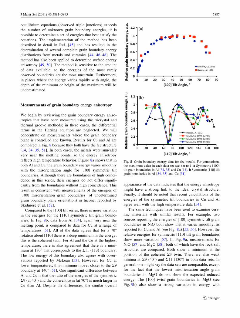
reflects high temperature behavior. Figure 8a shows that inboth Al and Cu, the grain boundary energy varies smoothly

with the misorientation angle for [100] symmetric tilt

boundaries. Although there are boundaries of high coinci-dence in this series, their energies do not differ signifi-

cantly from the boundaries without high coincidence. This

result is consistent with measurements of the energies of[100] misorientation grain boundaries (of undetermined

grain boundary plane orientation) in Inconel reported by

Skidmore et al. [52].Compared to the [100] tilt series, there is more variation

in the energies for the [110] symmetric tilt grain bound-

aries. In Fig. 8b, data from Al [34], again very near themelting point, is compared to data for Cu at a range of

temperatures [51]. All of the data agrees that for a 70"rotation about [110] there is a deep minimum in the energy;this is the coherent twin. For Al and the Cu at the highest

temperature, there is also agreement that there is a mini-

mum at 130" that corresponds to the R11 (113) boundary.The low energy of this boundary also agrees with obser-

vations reported by McLean [53]. However, for Cu at

lower temperatures, this minimum moves closer to the R9boundary at 140" [51]. One significant difference between

Al and Cu is that the ratio of the energies of the symmetric

R9 (at 40") and the coherent twin (at 70") is much larger inCu than Al. Despite the differences, the similar overall

appearance of the data indicates that the energy anisotropy

might have a strong link to the ideal crystal structure.

Finally, it should be noted that recent calculations of theenergies of the symmetric tilt boundaries in Cu and Al

agree well with the high temperature data [54].The same techniques have been used to examine cera-

mic materials with similar results. For example, two

sources reporting the energies of [100] symmetric tilt grainboundaries in NiO both show that it varies smoothly, as

reported for Cu and Al (see Fig. 8a) [55, 56]. However, the

relative energies for symmetric [110] tilt grain boundariesshow more variation [57]. In Fig. 9a, measurements for

NiO [57] and MgO [58], both of which have the rock salt

structure, are compared. Both show a minimum at theposition of the coherent R3 twin. There are also weak

minima at R9 (40") and R11 (130") in both data sets. In

general, one might say the data sets are comparable, exceptfor the fact that the lowest misorientation angle grain

boundaries in MgO do not show the expected reduced

energy. The [100] twist grain boundaries in MgO (seeFig. 9b) also show a strong variation in energy with

Fig. 8 Grain boundary energy data for fcc metals. For comparison,the maximum value in each data set was set to 1. a Symmetric [100]tilt grain boundaries in Al [34, 35] and Cu [14]. b Symmetric [110] tiltgrain boundaries in Al [34, 35] and Cu [51]

J Mater Sci (2011) 46:5881–5895 5887

123

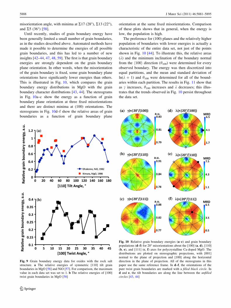
misorientation angle, with minima at R17 (28"), R13 (22"),and R5 (36") [58].

Until recently, studies of grain boundary energy have

been generally limited a small number of grain boundaries,

as in the studies described above. Automated methods havemade it possible to determine the energies of all possible

grain boundaries, and this has led to a number of new

insights [42–44, 47, 48, 59]. The first is that grain boundaryenergies are strongly dependent on the grain boundary

plane orientation. In other words, when the misorientationof the grain boundary is fixed, some grain boundary plane

orientations have significantly lower energies than others.

This is illustrated in Fig. 10, which compares the grainboundary energy distributions in MgO with the grain

boundary character distributions [43, 44]. The stereograms

in Fig. 10a–c show the energy as a function of grainboundary plane orientation at three fixed misorientations

and there are distinct minima at (100) orientations. The

stereograms in Fig. 10d–f show the relative areas of grainboundaries as a function of grain boundary plane

orientation at the same fixed misorientations. Comparison

of these plots shows that in general, when the energy islow, the population is high.

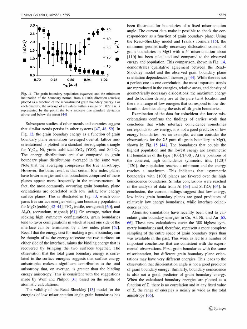
The preference for (100) planes and the relatively higher

population of boundaries with lower energies is actually acharacteristic of the entire data set, not just of the points

shown in Fig. 10 [44]. To illustrate this, the relative areas

(k) and the minimum inclination of the boundary normalfrom the h100i direction (h100) were determined for every

observed boundary. The energy was then discretized intoequal partitions, and the mean and standard deviation of

ln(k ? 1) and h100 were determined for all of the bound-

aries within each partition. The results in Fig. 11 show thatas c increases, h100 increases and k decreases; this illus-

trates that the trends observed in Fig. 10 persist throughout

the data set.

Fig. 9 Grain boundary energy data for oxides with the rock saltstructure. a The relative energies of symmetric [110] tilt grainboundaries in MgO [58] and NiO [57]. For comparison, the maximumvalue in each data set was set to 1. b The relative energies of [100]twist grain boundaries in MgO [58]

Fig. 10 Relative grain boundary energies (a–c) and grain boundarypopulations (d–f) for 20" misorientations about the [100] (a, d), [110](b, e), and [111] (c, f) axes for polycrystalline Ca-doped MgO. Thedistributions are plotted on stereographic projections, with [001]normal to the plane of projection and [100] along the horizontaldirection in the plane of projection. All of the stereograms in thispaper use the same reference frame. In d–f, the orientations of thepure twist grain boundaries are marked with a filled black circle. Ind and e, the tilt boundaries are along the line between the unfilledcircles [43, 44]

5888 J Mater Sci (2011) 46:5881–5895

123

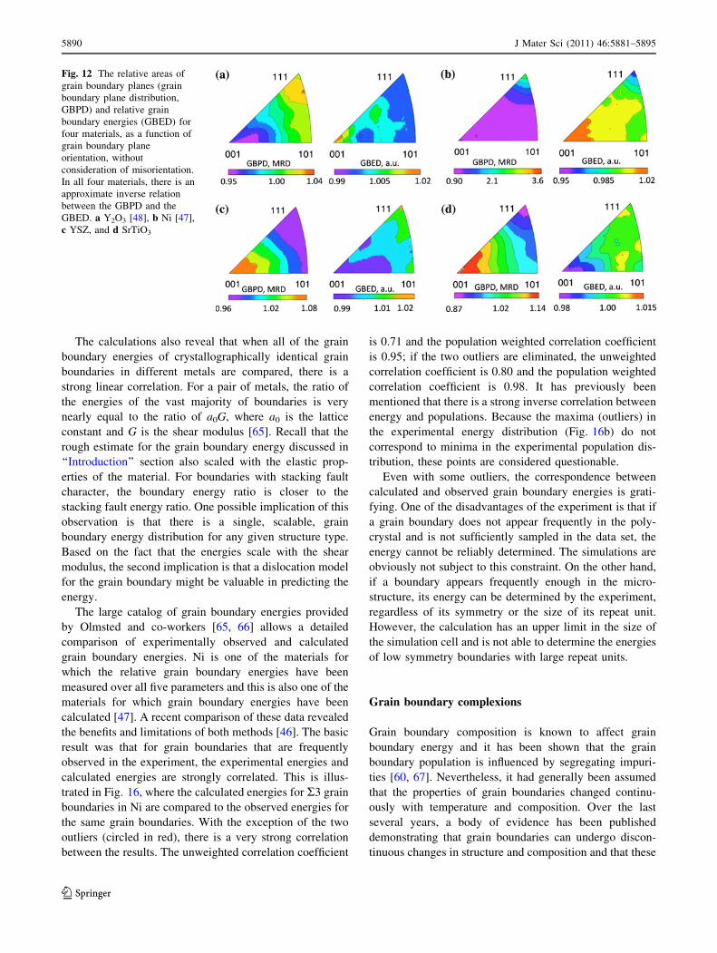
Subsequent studies of other metals and ceramics suggestthat similar trends persist in other systems [47, 48, 59]. In

Fig. 12, the grain boundary energy as a function of grain

boundary plane orientation (averaged over all lattice mis-orientations) is plotted in a standard stereographic triangle

for Y2O3, Ni, yttria stabilized ZrO2 (YSZ), and SrTiO3.

The energy distributions are also compared to grainboundary plane distributions averaged in the same way.

Note that the averaging compresses the true anisotropy.

However, the basic result is that certain low index planeshave lower energies and that boundaries comprised of these

planes appear more frequently in the microstructure. In

fact, the most commonly occurring grain boundary planeorientations are correlated with low index, low energy

surface planes. This is illustrated in Fig. 13, which com-pares free surface energies with grain boundary populations

for MgO (cubic) [42–44], TiO2 (rutile, tetragonal) [60], and

Al2O3 (corundum, trigonal) [61]. On average, rather thanseeking high symmetry configurations, grain boundaries

tend to favor configurations in which at least one side of the

interface can be terminated by a low index plane [62].Recall that the energy cost for making a grain boundary can

be thought of as the energy to create the two surfaces on

either side of the interface, minus the binding energy that isrecovered by bringing the two surfaces together. The

observation that the total grain boundary energy is corre-

lated to the surface energies suggests that surface energyanisotropies makes a significant contribution to the total

anisotropy that, on average, is greater than the binding

energy anisotropy. This is consistent with the suggestionsmade by Wolf and Philpot [31] based on the results of

atomistic calculations.

The validity of the Read–Shockley [13] model for theenergies of low misorientation angle grain boundaries has

been illustrated for boundaries of a fixed misorientation

angle. The current data make it possible to check the cor-respondence as a function of grain boundary plane. Using

the Read–Shockley model and Frank’s formula [15], the

minimum geometrically necessary dislocation content ofgrain boundaries in MgO with a 5" misorientation about

[110] has been calculated and compared to the observed

energy and population. This comparison, shown in Fig. 14,demonstrates qualitative agreement between the Read–

Shockley model and the observed grain boundary planeorientation dependence of the energy [44].While there is not

a perfect one-to-one correlation, the most important trends

are reproduced in the energies, relative areas, and density ofgeometrically necessary dislocations: the maximum energy

and dislocation density are at the pure twist location and

there is a range of low energies that correspond to low dis-location densities along the axis of tilt grain boundaries.

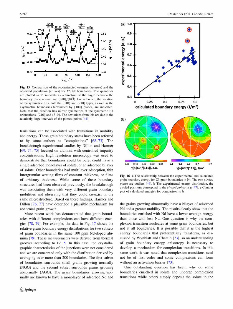
Examination of the data for coincident site lattice mis-

orientations confirms the findings of earlier work thatconcludes that while interface coincidence sometimes

corresponds to low energy, it is not a good predictor of low

energy boundaries. As an example, we can consider theobservations for the R5 pure tilt grain boundary in MgO,

shown in Fig. 15 [44]. The boundaries that couple the

highest population and the lowest energy are asymmetrictilt boundaries of the type {100}/{430}. At the positions of

the coherent, high coincidence symmetric tilts, {120}/

{120}, the population reaches a minimum and the energyreaches a maximum. This indicates that asymmetric

boundaries with {100} planes are favored over the high

coincidence boundaries. Similar conclusions were reachedin the analysis of data from Al [63] and SrTiO3 [64]. In

conclusion, the current findings suggest that low energy,

low index grain boundary planes are good predictors ofrelatively low energy boundaries, while interface coinci-

dence is not.

Atomistic simulations have recently been used to cal-culate grain boundary energies in Cu, Al, Ni, and Au [65,

66]. These new calculations cover the 388 highest sym-

metry boundaries and, therefore, represent a more completesampling of the entire space of grain boundary types than

was available in the past. This work as led to a number of

important conclusions that are consistent with the experi-mental observations. First, grain boundaries with the same

misorientation, but different grain boundary plane orien-

tations may have very different energies. This leads to theobservation that disorientation angle is not a good predictor

of grain boundary energy. Similarly, boundary coincidence

is also not a good predictor of grain boundary energy.When the calculated boundary energies are plotted as a

function of R, there is no correlation and at any fixed value

of R, the range of energies is nearly as wide as the totalanisotropy [66].

Fig. 11 The grain boundary population (squares) and the minimuminclination of the boundary normal from a h100i direction (circles)plotted as a function of the reconstructed grain boundary energy. Foreach quantity, the average of all values within a range of 0.022 a.u. isrepresented by the point; the bars indicate one standard deviationabove and below the mean [44]

J Mater Sci (2011) 46:5881–5895 5889

123

The calculations also reveal that when all of the grain

boundary energies of crystallographically identical grainboundaries in different metals are compared, there is a

strong linear correlation. For a pair of metals, the ratio of

the energies of the vast majority of boundaries is verynearly equal to the ratio of a0G, where a0 is the lattice

constant and G is the shear modulus [65]. Recall that the

rough estimate for the grain boundary energy discussed in‘‘Introduction’’ section also scaled with the elastic prop-

erties of the material. For boundaries with stacking faultcharacter, the boundary energy ratio is closer to the

stacking fault energy ratio. One possible implication of this

observation is that there is a single, scalable, grainboundary energy distribution for any given structure type.

Based on the fact that the energies scale with the shear

modulus, the second implication is that a dislocation modelfor the grain boundary might be valuable in predicting the

energy.

The large catalog of grain boundary energies providedby Olmsted and co-workers [65, 66] allows a detailed

comparison of experimentally observed and calculated

grain boundary energies. Ni is one of the materials forwhich the relative grain boundary energies have been

measured over all five parameters and this is also one of the

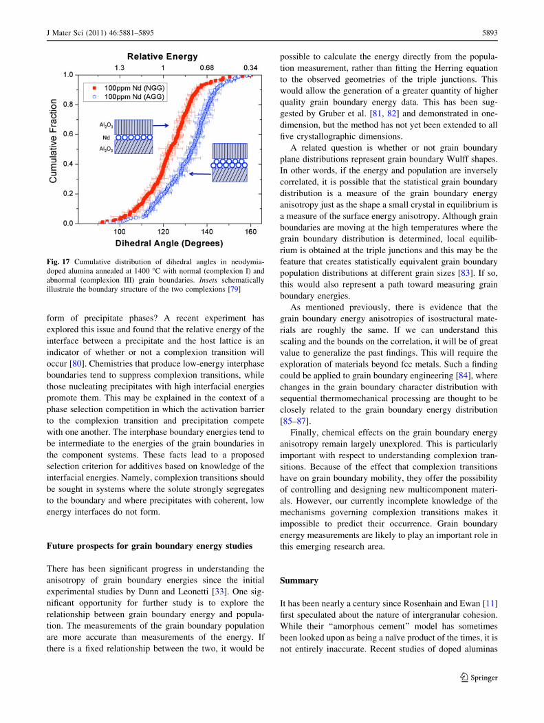
materials for which grain boundary energies have beencalculated [47]. A recent comparison of these data revealed

the benefits and limitations of both methods [46]. The basic

result was that for grain boundaries that are frequentlyobserved in the experiment, the experimental energies and

calculated energies are strongly correlated. This is illus-

trated in Fig. 16, where the calculated energies for R3 grainboundaries in Ni are compared to the observed energies for

the same grain boundaries. With the exception of the two

outliers (circled in red), there is a very strong correlationbetween the results. The unweighted correlation coefficient

is 0.71 and the population weighted correlation coefficient

is 0.95; if the two outliers are eliminated, the unweightedcorrelation coefficient is 0.80 and the population weighted

correlation coefficient is 0.98. It has previously been

mentioned that there is a strong inverse correlation betweenenergy and populations. Because the maxima (outliers) in

the experimental energy distribution (Fig. 16b) do not

correspond to minima in the experimental population dis-tribution, these points are considered questionable.

Even with some outliers, the correspondence betweencalculated and observed grain boundary energies is grati-

fying. One of the disadvantages of the experiment is that if

a grain boundary does not appear frequently in the poly-crystal and is not sufficiently sampled in the data set, the

energy cannot be reliably determined. The simulations are

obviously not subject to this constraint. On the other hand,if a boundary appears frequently enough in the micro-

structure, its energy can be determined by the experiment,

regardless of its symmetry or the size of its repeat unit.However, the calculation has an upper limit in the size of

the simulation cell and is not able to determine the energies

of low symmetry boundaries with large repeat units.

Grain boundary complexions

Grain boundary composition is known to affect grain

boundary energy and it has been shown that the grainboundary population is influenced by segregating impuri-

ties [60, 67]. Nevertheless, it had generally been assumed

that the properties of grain boundaries changed continu-ously with temperature and composition. Over the last

several years, a body of evidence has been published

demonstrating that grain boundaries can undergo discon-tinuous changes in structure and composition and that these

Fig. 12 The relative areas ofgrain boundary planes (grainboundary plane distribution,GBPD) and relative grainboundary energies (GBED) forfour materials, as a function ofgrain boundary planeorientation, withoutconsideration of misorientation.In all four materials, there is anapproximate inverse relationbetween the GBPD and theGBED. a Y2O3 [48], b Ni [47],c YSZ, and d SrTiO3

5890 J Mater Sci (2011) 46:5881–5895

123

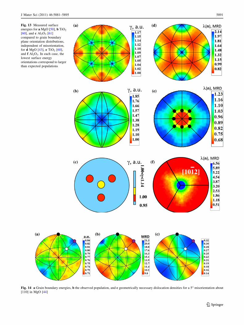
Fig. 13 Measured surfaceenergies for aMgO [50], b TiO2

[60], and c Al2O3 [61]compared to grain boundaryplane orientation distributions,independent of misorientation,for d MgO [43], e TiO2 [60],and f Al2O3. In each case, thelowest surface energyorientations correspond to largerthan expected populations

Fig. 14 a Grain boundary energies, b the observed population, and c geometrically necessary dislocation densities for a 5" misorientation about[110] in MgO [44]

J Mater Sci (2011) 46:5881–5895 5891

123

transitions can be associated with transitions in mobility

and energy. These grain boundary states have been referredto by some authors as ‘‘complexions’’ [68–73]. The

breakthrough experimental studies by Dillon and Harmer

[69, 74, 75] focused on alumina with controlled impurityconcentrations. High resolution microscopy was used to

demonstrate that boundaries could be pure, could have a

single adsorbed monolayer of solute, or an adsorbed bilayerof solute. Other boundaries had multilayer adsorption, thin

intergranular wetting films of constant thickness, or films

of arbitrary thickness. While some of these boundarystructures had been observed previously, the breakthrough

was associating them with very different grain boundary

mobilities and observing that they could co-exist in thesame microstructure. Based on these findings, Harmer and

Dillon [76, 77] have described a plausible mechanism for

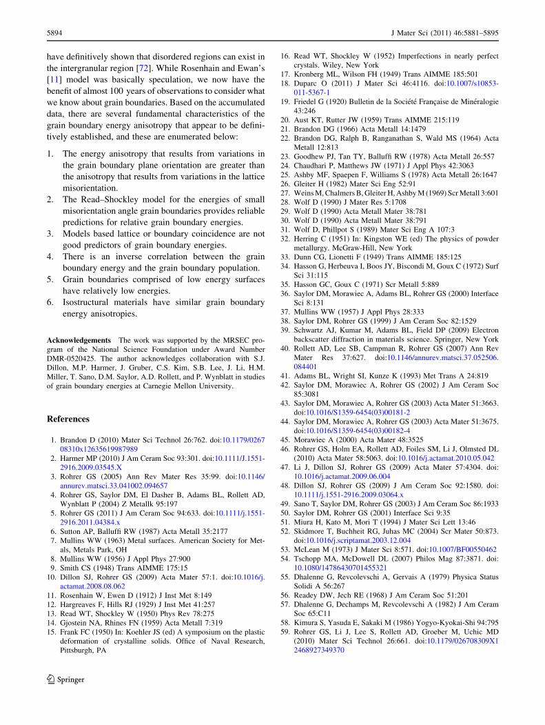
abnormal grain growth.More recent work has demonstrated that grain bound-

aries with different complexions can have different ener-

gies [78, 79]. For example, the data in Fig. 17 shows therelative grain boundary energy distributions for two subsets

of grain boundaries in the same 100 ppm Nd-doped alu-

mina [79]. These measurements were derived from thermalgrooves according to Eq. 5. In this case, the crystallo-

graphic characteristics of the junctions were not considered

and we are concerned only with the distribution derived byaveraging over more than 200 boundaries. The first subset

of boundaries surrounds small grains growing normally

(NGG) and the second subset surrounds grains growingabnormally (AGG). The grain boundaries growing nor-

mally are known to have a monolayer of adsorbed Nd and

the grains growing abnormally have a bilayer of adsorbed

Nd and a greater mobility. The results clearly show that theboundaries enriched with Nd have a lower average energy

than those with less Nd. One question is why the com-

plexion transition nucleates at some grain boundaries, butnot at all boundaries. It is possible that it is the highest

energy boundaries that preferentially transform, as dis-

cussed by Wynblatt and Chatain [73], so an understandingof grain boundary energy anisotropy is necessary to

develop a mechanism for complexion transitions. In this

same work, it was noted that complexion transitions neednot be of first order and some complexions can form

without an activation barrier [73].One outstanding question has been, why do some

boundaries enriched in solute and undergo complexion

transitions while others simply deposit the solute in the

Fig. 15 Comparison of the reconstructed energies (squares) and theobserved population (circles) for R5 tilt boundaries. The quantitiesare plotted in 5" intervals as a function of the angle between theboundary plane normal and 010# $=#04!3$. For reference, the locationof the symmetric tilts, both the {310} and {210} types, as well as theasymmetric boundaries terminated by {100} planes, are indicated.Note that the function has mirror symmetries at the symmetric tiltorientations, {210} and {310}. The deviations from this are due to therelatively large intervals of the plotted points [44]

Fig. 16 a The relationship between the experimental and calculatedgrain boundary energy for R3 grain boundaries in Ni. The two circledpoints are outliers [46]. b The experimental energy distribution, thecircled positions correspond to the circled points in a [47]. c Contourplot of calculated energies for comparison to b

5892 J Mater Sci (2011) 46:5881–5895

123

form of precipitate phases? A recent experiment hasexplored this issue and found that the relative energy of the

interface between a precipitate and the host lattice is an

indicator of whether or not a complexion transition willoccur [80]. Chemistries that produce low-energy interphase

boundaries tend to suppress complexion transitions, while

those nucleating precipitates with high interfacial energiespromote them. This may be explained in the context of a

phase selection competition in which the activation barrier

to the complexion transition and precipitation competewith one another. The interphase boundary energies tend to

be intermediate to the energies of the grain boundaries in

the component systems. These facts lead to a proposedselection criterion for additives based on knowledge of the

interfacial energies. Namely, complexion transitions should

be sought in systems where the solute strongly segregatesto the boundary and where precipitates with coherent, low

energy interfaces do not form.

Future prospects for grain boundary energy studies

There has been significant progress in understanding the

anisotropy of grain boundary energies since the initial

experimental studies by Dunn and Leonetti [33]. One sig-nificant opportunity for further study is to explore the

relationship between grain boundary energy and popula-tion. The measurements of the grain boundary population

are more accurate than measurements of the energy. If

there is a fixed relationship between the two, it would be

possible to calculate the energy directly from the popula-

tion measurement, rather than fitting the Herring equationto the observed geometries of the triple junctions. This

would allow the generation of a greater quantity of higher

quality grain boundary energy data. This has been sug-gested by Gruber et al. [81, 82] and demonstrated in one-

dimension, but the method has not yet been extended to all

five crystallographic dimensions.A related question is whether or not grain boundary

plane distributions represent grain boundary Wulff shapes.In other words, if the energy and population are inversely

correlated, it is possible that the statistical grain boundary

distribution is a measure of the grain boundary energyanisotropy just as the shape a small crystal in equilibrium is

a measure of the surface energy anisotropy. Although grain

boundaries are moving at the high temperatures where thegrain boundary distribution is determined, local equilib-

rium is obtained at the triple junctions and this may be the

feature that creates statistically equivalent grain boundarypopulation distributions at different grain sizes [83]. If so,

this would also represent a path toward measuring grain

boundary energies.As mentioned previously, there is evidence that the

grain boundary energy anisotropies of isostructural mate-

rials are roughly the same. If we can understand thisscaling and the bounds on the correlation, it will be of great

value to generalize the past findings. This will require the

exploration of materials beyond fcc metals. Such a findingcould be applied to grain boundary engineering [84], where

changes in the grain boundary character distribution with

sequential thermomechanical processing are thought to beclosely related to the grain boundary energy distribution

[85–87].

Finally, chemical effects on the grain boundary energyanisotropy remain largely unexplored. This is particularly

important with respect to understanding complexion tran-

sitions. Because of the effect that complexion transitionshave on grain boundary mobility, they offer the possibility

of controlling and designing new multicomponent materi-

als. However, our currently incomplete knowledge of themechanisms governing complexion transitions makes it

impossible to predict their occurrence. Grain boundary

energy measurements are likely to play an important role inthis emerging research area.

Summary

It has been nearly a century since Rosenhain and Ewan [11]first speculated about the nature of intergranular cohesion.

While their ‘‘amorphous cement’’ model has sometimes

been looked upon as being a naıve product of the times, it isnot entirely inaccurate. Recent studies of doped aluminas

Fig. 17 Cumulative distribution of dihedral angles in neodymia-doped alumina annealed at 1400 "C with normal (complexion I) andabnormal (complexion III) grain boundaries. Insets schematicallyillustrate the boundary structure of the two complexions [79]

J Mater Sci (2011) 46:5881–5895 5893

123

have definitively shown that disordered regions can exist in

the intergranular region [72]. While Rosenhain and Ewan’s[11] model was basically speculation, we now have the

benefit of almost 100 years of observations to consider what

we know about grain boundaries. Based on the accumulateddata, there are several fundamental characteristics of the

grain boundary energy anisotropy that appear to be defini-

tively established, and these are enumerated below:

1. The energy anisotropy that results from variations in

the grain boundary plane orientation are greater thanthe anisotropy that results from variations in the lattice

misorientation.

2. The Read–Shockley model for the energies of smallmisorientation angle grain boundaries provides reliable

predictions for relative grain boundary energies.

3. Models based lattice or boundary coincidence are notgood predictors of grain boundary energies.

4. There is an inverse correlation between the grainboundary energy and the grain boundary population.

5. Grain boundaries comprised of low energy surfaces

have relatively low energies.6. Isostructural materials have similar grain boundary

energy anisotropies.

Acknowledgements The work was supported by the MRSEC pro-gram of the National Science Foundation under Award NumberDMR-0520425. The author acknowledges collaboration with S.J.Dillon, M.P. Harmer, J. Gruber, C.S. Kim, S.B. Lee, J. Li, H.M.Miller, T. Sano, D.M. Saylor, A.D. Rollett, and P. Wynblatt in studiesof grain boundary energies at Carnegie Mellon University.

References

1. Brandon D (2010) Mater Sci Technol 26:762. doi:10.1179/026708310x12635619987989

2. Harmer MP (2010) J Am Ceram Soc 93:301. doi:10.1111/J.1551-2916.2009.03545.X

3. Rohrer GS (2005) Ann Rev Mater Res 35:99. doi:10.1146/annurev.matsci.33.041002.094657

4. Rohrer GS, Saylor DM, El Dasher B, Adams BL, Rollett AD,Wynblatt P (2004) Z Metallk 95:197

5. Rohrer GS (2011) J Am Ceram Soc 94:633. doi:10.1111/j.1551-2916.2011.04384.x

6. Sutton AP, Balluffi RW (1987) Acta Metall 35:21777. Mullins WW (1963) Metal surfaces. American Society for Met-

als, Metals Park, OH8. Mullins WW (1956) J Appl Phys 27:9009. Smith CS (1948) Trans AIMME 175:15

10. Dillon SJ, Rohrer GS (2009) Acta Mater 57:1. doi:10.1016/j.actamat.2008.08.062

11. Rosenhain W, Ewen D (1912) J Inst Met 8:14912. Hargreaves F, Hills RJ (1929) J Inst Met 41:25713. Read WT, Shockley W (1950) Phys Rev 78:27514. Gjostein NA, Rhines FN (1959) Acta Metall 7:31915. Frank FC (1950) In: Koehler JS (ed) A symposium on the plastic

deformation of crystalline solids. Office of Naval Research,Pittsburgh, PA

16. Read WT, Shockley W (1952) Imperfections in nearly perfectcrystals. Wiley, New York

17. Kronberg ML, Wilson FH (1949) Trans AIMME 185:50118. Duparc O (2011) J Mater Sci 46:4116. doi:10.1007/s10853-

011-5367-119. Friedel G (1920) Bulletin de la Societe Francaise de Mineralogie

43:24620. Aust KT, Rutter JW (1959) Trans AIMME 215:11921. Brandon DG (1966) Acta Metall 14:147922. Brandon DG, Ralph B, Ranganathan S, Wald MS (1964) Acta

Metall 12:81323. Goodhew PJ, Tan TY, Balluffi RW (1978) Acta Metall 26:55724. Chaudhari P, Matthews JW (1971) J Appl Phys 42:306325. Ashby MF, Spaepen F, Williams S (1978) Acta Metall 26:164726. Gleiter H (1982) Mater Sci Eng 52:9127. WeinsM,Chalmers B,Gleiter H,AshbyM (1969) ScrMetall 3:60128. Wolf D (1990) J Mater Res 5:170829. Wolf D (1990) Acta Metall Mater 38:78130. Wolf D (1990) Acta Metall Mater 38:79131. Wolf D, Phillpot S (1989) Mater Sci Eng A 107:332. Herring C (1951) In: Kingston WE (ed) The physics of powder

metallurgy. McGraw-Hill, New York33. Dunn CG, Lionetti F (1949) Trans AIMME 185:12534. Hasson G, Herbeuva I, Boos JY, Biscondi M, Goux C (1972) Surf

Sci 31:11535. Hasson GC, Goux C (1971) Scr Metall 5:88936. Saylor DM, Morawiec A, Adams BL, Rohrer GS (2000) Interface

Sci 8:13137. Mullins WW (1957) J Appl Phys 28:33338. Saylor DM, Rohrer GS (1999) J Am Ceram Soc 82:152939. Schwartz AJ, Kumar M, Adams BL, Field DP (2009) Electron

backscatter diffraction in materials science. Springer, New York40. Rollett AD, Lee SB, Campman R, Rohrer GS (2007) Ann Rev

Mater Res 37:627. doi:10.1146/annurev.matsci.37.052506.084401

41. Adams BL, Wright SI, Kunze K (1993) Met Trans A 24:81942. Saylor DM, Morawiec A, Rohrer GS (2002) J Am Ceram Soc

85:308143. Saylor DM, Morawiec A, Rohrer GS (2003) Acta Mater 51:3663.

doi:10.1016/S1359-6454(03)00181-244. Saylor DM, Morawiec A, Rohrer GS (2003) Acta Mater 51:3675.

doi:10.1016/S1359-6454(03)00182-445. Morawiec A (2000) Acta Mater 48:352546. Rohrer GS, Holm EA, Rollett AD, Foiles SM, Li J, Olmsted DL

(2010) Acta Mater 58:5063. doi:10.1016/j.actamat.2010.05.04247. Li J, Dillon SJ, Rohrer GS (2009) Acta Mater 57:4304. doi:

10.1016/j.actamat.2009.06.00448. Dillon SJ, Rohrer GS (2009) J Am Ceram Soc 92:1580. doi:

10.1111/j.1551-2916.2009.03064.x49. Sano T, Saylor DM, Rohrer GS (2003) J Am Ceram Soc 86:193350. Saylor DM, Rohrer GS (2001) Interface Sci 9:3551. Miura H, Kato M, Mori T (1994) J Mater Sci Lett 13:4652. Skidmore T, Buchheit RG, Juhas MC (2004) Scr Mater 50:873.

doi:10.1016/j.scriptamat.2003.12.00453. McLean M (1973) J Mater Sci 8:571. doi:10.1007/BF0055046254. Tschopp MA, McDowell DL (2007) Philos Mag 87:3871. doi:

10.1080/1478643070145532155. Dhalenne G, Revcolevschi A, Gervais A (1979) Physica Status

Solidi A 56:26756. Readey DW, Jech RE (1968) J Am Ceram Soc 51:20157. Dhalenne G, Dechamps M, Revcolevschi A (1982) J Am Ceram

Soc 65:C1158. Kimura S, Yasuda E, Sakaki M (1986) Yogyo-Kyokai-Shi 94:79559. Rohrer GS, Li J, Lee S, Rollett AD, Groeber M, Uchic MD

(2010) Mater Sci Technol 26:661. doi:10.1179/026708309X12468927349370

5894 J Mater Sci (2011) 46:5881–5895

123

60. Pang Y, Wynblatt P (2006) J Am Ceram Soc 89:666. doi:10.1111/j.1551-2916.2005.007993x

61. Kitayama M, Glaeser AM (2002) J Am Ceram Soc 85:61162. Saylor DM, El Dasher B, Pang Y et al (2004) J Am Ceram Soc

87:72463. Saylor DM, El Dasher BS, Rollett AD, Rohrer GS (2004) Acta

Mater 52:3649. doi:10.1016/j.actamat.2004.04.01864. Saylor DM, El Dasher B, Sano T, Rohrer GS (2004) J Am Ceram

Soc 87:67065. Holm EA, Olmsted DL, Foiles SM (2010) Scr Mater 63:905. doi:

10.1016/j.scriptamat.2010.06.04066. Olmsted DL, Foiles SM, Holm EA (2009) Acta Mater 57:3694.

doi:10.1016/j.actamat.2009.04.00767. Papillon F, Rohrer GS, Wynblatt P (2009) J Am Ceram Soc

92:3044. doi:10.1111/j.1551-2916.2009.03327.x68. Baram M, Chatain D, Kaplan WD (2011) Science 332:206. doi:

10.1126/science.120159669. Dillon SJ, Tang M, Carter WC, Harmer MP (2007) Acta Mater

55:6208. doi:10.1016/j.actamat.2007.07.02970. Tang M, Carter WC, Cannon RM (2006) Phys Rev Lett 97:4. doi:

07550210.1103/PhysRevLett.97.07550271. Tang M, Carter WC, Cannon RM (2006) J Mater Sci 41:7691.

doi:10.1007/s10853-006-0608-472. Tang M, Carter WC, Cannon RM (2006) Phys Rev B 73:14. doi:

02410210.1103/PhysRevB.73.02410273. Wynblatt P, Chatain D (2008) Mater Sci Eng A 495:119. doi:

10.1016/j.msea.2007.09.09174. Dillon SJ, Harmer MP (2007) Acta Mater 55:5247. doi:

10.1016/j.actamat.2007.04.051

75. Dillon SJ, Harmer MP (2007) J Am Ceram Soc 90:996. doi:10.1111/j.1551-2916.2007.01512.x

76. Dillon SJ, Harmer MP (2008) J Am Ceram Soc 91:2304. doi:10.1111/j.1551-2916.2008.02454.x

77. Dillon SJ, Harmer MP (2008) J Am Ceram Soc 91:2314. doi:10.1111/j.1551-2916.2008.02432.x

78. Dillon SJ, Miller H, Harmer MP, Rohrer GS (2010) Int J MaterRes 101:50. doi:10.3139/146.110253

79. Dillon SJ, Harmer MP, Rohrer GS (2010) J Am Ceram Soc93:1796. doi:10.1111/j.1551-2916.2010.03642.x

80. Dillon SJ, Harmer MP, Rohrer GS (2010) Acta Mater 58:5097.doi:10.1016/j.actamat.2010.05.045

81. Gruber J, Rollett AD, Rohrer GS (2010) Acta Mater 58:14. doi:10.1016/j.actamat.2009.08.032

82. Gruber J, Miller HM, Hoffmann TD, Rohrer GS, Rollett AD(2009) Acta Mater 57:6102. doi:10.1016/j.actamat.2009.08.036

83. Gruber J, George DC, Kuprat AP, Rohrer GS, Rollett AD (2005)Scr Mater 53:351. doi:10.1016/j.scriptamat.2005.04.004

84. Watanabe T (2011) J Mater Sci 46:4095. doi:10.1007/s10853-011-5393-z

85. Randle V, Rohrer GS, Miller HM, Coleman M, Owen GT (2008)Acta Mater 56:2363. doi:10.1016/j.actamat.2008.01.039

86. Rohrer GS, Randle V, Kim CS, Hu Y (2006) Acta Mater 54:4489.doi:10.1016/j.actamat.2006.05.035

87. Kim CS, Hu Y, Rohrer GS, Randle V (2005) Scr Mater 52:633.doi:10.1016/j.scriptamat.2004.11.025

J Mater Sci (2011) 46:5881–5895 5895

123