Canada Employment and Labour market - December 2016 - analysis and commentary
Upload
truongphucCategory
view
215download
2
Graduate Labour Market Analysis in
Malaysia
Diana Binti Abdul Wahab
Submitted in accordance with the requirements for the degree of
Doctor of Philosophy
The University of Leeds
Leeds University Business School
Department of Economics
February 2017

The candidate confirms that the work submitted is her own and that appropriate
credit has been given where reference has been made to the work of others.
This copy has been supplied on the understanding that it is copyright material and
that no quotation from the thesis may be published without proper
acknowledgement.
c© 2017 The University of Leeds and Diana Binti Abdul Wahab
ii

AbstractThis thesis studies several aspects related to graduate employment in Malaysia. The
first chapter examines graduate’s transition from education to work which includes
the analysis of the first destination choice after study and occupational types using
multinomial logit model. Within each occupational category, we use Fairlie’s non-
linear decomposition technique to compute the differences in the participation rate
between gender and ethnic groups. Women and Malay’s under-representation in su-
perior occupational types are largely due to their choice of less attractive courses that
are associated with low market demand. The second chapter analyzes the wage dif-
ferentials between the public-private sectors, gender and ethnic groups. The earning
equation is adjusted to account for the sample selection bias due to the participation
rate. We use the Oaxaca-Blinder decomposition technique to compute the wage dif-
ferences between the groups. The difference in the sectoral wage is non-significant,
and there is no evidence of wage differential in the public sector. Gender and ethnic
pay gap only occur in the private sector where male and Chinese consistently earn
higher. The third chapter explores another dimensions of graduate’s transition from
education to work. First, we found that higher ability graduates are more inclined
to migrate in order to maximize their employment prospects as well as compensat-
ing for their superior human capital. Indeed, graduate’s migration results in higher
earning but not necessarily reduce education-job mismatch. Second, graduates who
possess better characteristics took longer to obtain their first job but they ended up
with superior occupational types and higher earning. Yet, social attributes such as
being a male, a Chinese, or originating from an urban state increases the probabil-
ity for faster transition from education to work. Third, using a pseudo-panel data
and controlling for cohort heterogeneity shows that the remaining variables that
significantly affect earning are family income and locality.
iii

iv

Acknowledgements
All praise is due to Allah for His Mercy and Guidance.
My study is made possible with the funding from the Ministry of Higher Education
through the University of Malaya.
I am especially grateful to my supervisors Dr. Kausik Chaudhuri and Dr. Luisa
Zanchi for their helpful suggestions and advice throughout my study; and for their
trust in me against all odds even though I had only two years to come out with this
thesis. To Dr. Rohana Jani for her persistent support and inspiration, and also for
providing me with the data which becomes the essential part of this thesis.
My deepest gratitude to my mother who has fought for our education while she
was denied entry to the best school in the country during her childhood due to
poverty. To my late father, who passed away during my final year, making it the
most difficult journey home across the continents. To my husband, for endless and
tireless support throughout. To my toddler son, for being the source of joy when
life gets most difficult. Finally, to all families and friends who make life colorful.
v

vi

Contents
Abstract . . . . . . . . . . . . . . . . . . . . . . . . . . . . . . . . . . . . . iii
Acknowledgements . . . . . . . . . . . . . . . . . . . . . . . . . . . . . . . v
Contents . . . . . . . . . . . . . . . . . . . . . . . . . . . . . . . . . . . . . vii
List of figures . . . . . . . . . . . . . . . . . . . . . . . . . . . . . . . . . . xi
List of tables . . . . . . . . . . . . . . . . . . . . . . . . . . . . . . . . . . xii
1 Introduction 1
1.1 Thesis structure . . . . . . . . . . . . . . . . . . . . . . . . . . . . . . 1
1.2 Overview of Malaysia . . . . . . . . . . . . . . . . . . . . . . . . . . . 4
1.3 Educational system in Malaysia . . . . . . . . . . . . . . . . . . . . . 8
1.4 Description of the Graduate Tracer Study data. . . . . . . . . . . . . 11
2 Graduate’s first destination choice and employment. 19
2.1 Introduction. . . . . . . . . . . . . . . . . . . . . . . . . . . . . . . . 19
2.2 Literature review. . . . . . . . . . . . . . . . . . . . . . . . . . . . . . 22
2.3 Data. . . . . . . . . . . . . . . . . . . . . . . . . . . . . . . . . . . . . 30
vii
2.4 Econometric framework. . . . . . . . . . . . . . . . . . . . . . . . . . 39
2.4.1 Modelling graduate employment outcomes. . . . . . . . . . . . 39
2.4.2 Modelling gender differences in employment outcomes. . . . . 42
2.5 Empirical results. . . . . . . . . . . . . . . . . . . . . . . . . . . . . . 44
2.5.1 Graduate’s first destination and job characteristics. . . . . . . 44
2.5.2 Gender differences in employment pattern. . . . . . . . . . . . 55
2.5.3 Gender differences within course of study. . . . . . . . . . . . 62
2.5.4 Gender segregation by industry. . . . . . . . . . . . . . . . . . 66
2.5.5 Ethnic differences by industry. . . . . . . . . . . . . . . . . . . 70
2.6 Conclusion. . . . . . . . . . . . . . . . . . . . . . . . . . . . . . . . . 75
2.7 Appendix. . . . . . . . . . . . . . . . . . . . . . . . . . . . . . . . . . 79
3 Wage differentials across sectors, gender, and ethnic groups. 83
3.1 Introduction. . . . . . . . . . . . . . . . . . . . . . . . . . . . . . . . 83
3.2 Background and previous researches. . . . . . . . . . . . . . . . . . . 87
3.2.1 Earning function, equalising difference, and wage determination. 87
3.2.2 Public-private sector labour market. . . . . . . . . . . . . . . . 89
3.2.3 Gender pay gap . . . . . . . . . . . . . . . . . . . . . . . . . . 92
3.2.4 Ethnic wage gap. . . . . . . . . . . . . . . . . . . . . . . . . . 96
3.2.5 Full time wage premium. . . . . . . . . . . . . . . . . . . . . . 100
3.3 Data. . . . . . . . . . . . . . . . . . . . . . . . . . . . . . . . . . . . . 101
viii
3.4 Econometric framework. . . . . . . . . . . . . . . . . . . . . . . . . . 105
3.5 Empirical results. . . . . . . . . . . . . . . . . . . . . . . . . . . . . . 113
3.5.1 Public-private wage differentials. . . . . . . . . . . . . . . . . 113
3.5.2 Gender pay gap. . . . . . . . . . . . . . . . . . . . . . . . . . 129
3.5.3 Wage differential by ethnic groups. . . . . . . . . . . . . . . . 138
3.5.4 Full time pay premium. . . . . . . . . . . . . . . . . . . . . . 143
3.6 Conclusion. . . . . . . . . . . . . . . . . . . . . . . . . . . . . . . . . 145
3.7 Appendix. . . . . . . . . . . . . . . . . . . . . . . . . . . . . . . . . . 149
4 Interregional migration, time to obtain the first job, and cohorts
earning. 163
4.1 Introduction. . . . . . . . . . . . . . . . . . . . . . . . . . . . . . . . 163
4.2 Interregional migration and education-job mismatch. . . . . . . . . . 167
4.2.1 Graduates migration patterns. . . . . . . . . . . . . . . . . . . 174
4.2.2 Modelling migration and education-job mismatch. . . . . . . . 180
4.2.3 Summary on migration pattern and education-job mismatch. . 197
4.3 Transition time from higher education to employment. . . . . . . . . 198
4.3.1 Survival analysis of transition. . . . . . . . . . . . . . . . . . . 200
4.3.2 The transition from university to work in Malaysia. . . . . . . 203
4.3.3 Summary on transition time to gain employment. . . . . . . . 211
4.4 Estimating graduate earnings - pseudo-panel approach. . . . . . . . . 212
ix

4.4.1 Fixed effects ordered logit model of graduates earnings. . . . . 219
4.4.2 FEOL result. . . . . . . . . . . . . . . . . . . . . . . . . . . . 222
4.5 Conclusion. . . . . . . . . . . . . . . . . . . . . . . . . . . . . . . . . 226
4.6 Appendix. . . . . . . . . . . . . . . . . . . . . . . . . . . . . . . . . . 227
5 Conclusion 229
5.1 Summary of results . . . . . . . . . . . . . . . . . . . . . . . . . . . . 229
5.2 Limitation and future recommendation . . . . . . . . . . . . . . . . . 234
x

List of Figures
1.1 The states in Malaysia. The map is constructed for labelling purpose
only, ignoring the real distance between the Peninsular states and the
Borneo states as well as actual size comparison. . . . . . . . . . . . . 4
1.2 Total number of graduates produced by participating higher educa-
tion institutions in Malaysia including all levels of studies for the year
2013. . . . . . . . . . . . . . . . . . . . . . . . . . . . . . . . . . . . . 10
xi

xii
List of Tables
1.1 GDP Per Capita by State, 2012 - 2013 in Ringgit Malaysia (RM) . . 6
1.2 Urbanisation and population distribution by state . . . . . . . . . . . 7
1.3 Total number of graduates produced by Malaysia higher learning in-
stitutions in 2013 based on awarded certificates. . . . . . . . . . . . . 9
1.4 Data description - the Graduate Tracer Study . . . . . . . . . . . . . 14
1.5 Descriptive statistics - the Graduate Tracer Study. . . . . . . . . . . . 17
2.1 Summary statistics for the unemployed and employed graduates. . . 31
2.2 Summary statistics of the job characteristics among the employed
graduates. . . . . . . . . . . . . . . . . . . . . . . . . . . . . . . . . . 34
2.3 Employment patterns by universities. . . . . . . . . . . . . . . . . . 35
2.3 Employment patterns by universities. . . . . . . . . . . . . . . . . . . 36
2.4 Employment patterns by courses of study. . . . . . . . . . . . . . . . 37
2.5 Employment outcomes among graduates. . . . . . . . . . . . . . . . 49
2.6 Self-employment and working with family. . . . . . . . . . . . . . . . 52
2.7 Job levels among graduates. . . . . . . . . . . . . . . . . . . . . . . . 54
xiii
2.8 Gender differences in the employment outcomes. . . . . . . . . . . . 56
2.9 Gender differences in the job levels. . . . . . . . . . . . . . . . . . . 58
2.10 Gender differences in the job groups. . . . . . . . . . . . . . . . . . . 60
2.11 Gender differences within each course of study - full time employment 64
2.12 Gender differences within each course of study - part time employ-
ment. . . . . . . . . . . . . . . . . . . . . . . . . . . . . . . . . . . . 65
2.13 Gender differences within each industry - full time employment. . . . 67
2.14 Gender differences within each industry - part time employment. . . 69
2.15 Ethnic differences within each industry. . . . . . . . . . . . . . . . . 72
2.16 Ethnic differences within each industry. . . . . . . . . . . . . . . . . 73
2.17 Ethnic differences within each industry. . . . . . . . . . . . . . . . . 74
2.18 Employment outcomes among graduates. . . . . . . . . . . . . . . . 80
2.19 Job levels among graduates. . . . . . . . . . . . . . . . . . . . . . . . 81
3.1 Public and private sector wage distribution among sample graduates. 101
3.2 Graduate’s employment, gender, and income level by courses of study. 103
3.3 Gender and income level by industries. . . . . . . . . . . . . . . . . . 104
3.4 Estimation results of participation choice and public sector employ-
ment (marginal effects). . . . . . . . . . . . . . . . . . . . . . . . . . 114
3.5 Estimation results of graduate earnings in the public sector employ-
ment . . . . . . . . . . . . . . . . . . . . . . . . . . . . . . . . . . . 119
xiv
3.6 Estimation results of graduate earnings in the private sector employ-
ment . . . . . . . . . . . . . . . . . . . . . . . . . . . . . . . . . . . 121
3.7 Decomposition results for earning differentials in the public and pri-
vate sector employment. . . . . . . . . . . . . . . . . . . . . . . . . . 127
3.8 Decomposition results for gender pay gap in the public and private
sectors. . . . . . . . . . . . . . . . . . . . . . . . . . . . . . . . . . . 131
3.9 Decomposition results for gender pay gap within each industry. . . . . 135
3.10 Decomposition results for gender pay gap within each industry. . . . . 136
3.11 Decomposition results for gender pay gap within each industry. . . . . 137
3.12 Decomposition results for ethnic polarization in the public sector. . . 139
3.13 Decomposition results for ethnic polarization in the private sector. . 140
3.14 Decomposition results for public-private earning differentials within
each ethnic group. . . . . . . . . . . . . . . . . . . . . . . . . . . . . 142
3.15 Decomposition results for earning differential between full time / part
time workers. . . . . . . . . . . . . . . . . . . . . . . . . . . . . . . . 144
3.16 Estimation results of graduate earnings in the public sector employ-
ment . . . . . . . . . . . . . . . . . . . . . . . . . . . . . . . . . . . 150
3.17 Estimation results of graduate earnings in the private sector employ-
ment . . . . . . . . . . . . . . . . . . . . . . . . . . . . . . . . . . . 151
3.18 Estimation results of male graduate earnings . . . . . . . . . . . . . 152
3.19 Estimation results of female graduate earnings . . . . . . . . . . . . 155
3.20 Decomposition results for ethnic polarization in the public sector -
source of contribution. . . . . . . . . . . . . . . . . . . . . . . . . . . 158
xv
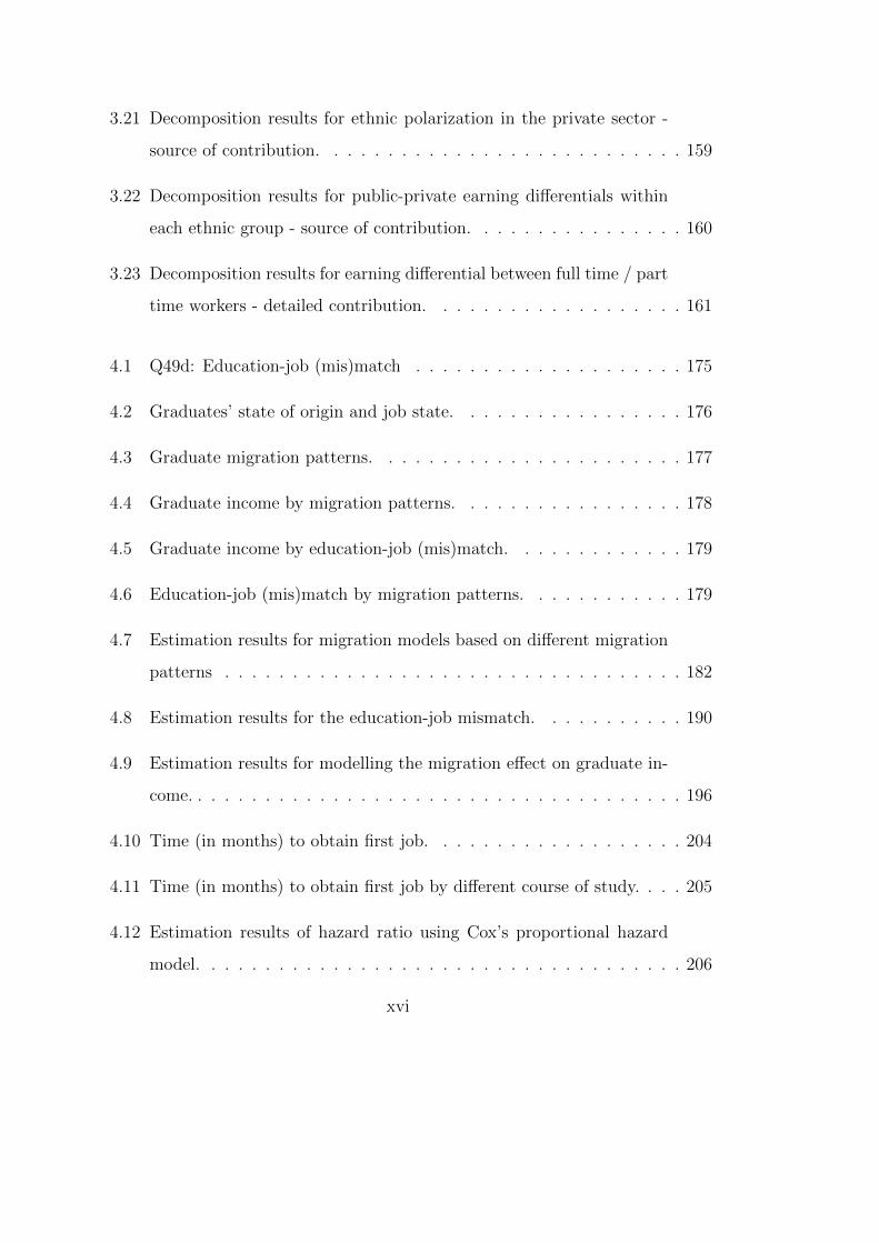
3.21 Decomposition results for ethnic polarization in the private sector -
source of contribution. . . . . . . . . . . . . . . . . . . . . . . . . . . 159
3.22 Decomposition results for public-private earning differentials within
each ethnic group - source of contribution. . . . . . . . . . . . . . . . 160
3.23 Decomposition results for earning differential between full time / part
time workers - detailed contribution. . . . . . . . . . . . . . . . . . . 161
4.1 Q49d: Education-job (mis)match . . . . . . . . . . . . . . . . . . . . 175
4.2 Graduates’ state of origin and job state. . . . . . . . . . . . . . . . . 176
4.3 Graduate migration patterns. . . . . . . . . . . . . . . . . . . . . . . 177
4.4 Graduate income by migration patterns. . . . . . . . . . . . . . . . . 178
4.5 Graduate income by education-job (mis)match. . . . . . . . . . . . . 179
4.6 Education-job (mis)match by migration patterns. . . . . . . . . . . . 179
4.7 Estimation results for migration models based on different migration
patterns . . . . . . . . . . . . . . . . . . . . . . . . . . . . . . . . . . 182
4.8 Estimation results for the education-job mismatch. . . . . . . . . . . 190
4.9 Estimation results for modelling the migration effect on graduate in-
come. . . . . . . . . . . . . . . . . . . . . . . . . . . . . . . . . . . . . 196
4.10 Time (in months) to obtain first job. . . . . . . . . . . . . . . . . . . 204
4.11 Time (in months) to obtain first job by different course of study. . . . 205
4.12 Estimation results of hazard ratio using Cox’s proportional hazard
model. . . . . . . . . . . . . . . . . . . . . . . . . . . . . . . . . . . . 206
xvi
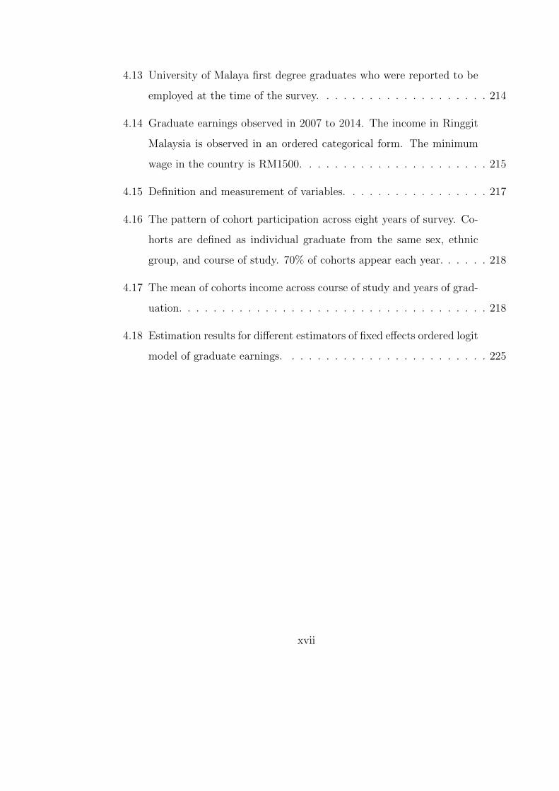
4.13 University of Malaya first degree graduates who were reported to be
employed at the time of the survey. . . . . . . . . . . . . . . . . . . . 214
4.14 Graduate earnings observed in 2007 to 2014. The income in Ringgit
Malaysia is observed in an ordered categorical form. The minimum
wage in the country is RM1500. . . . . . . . . . . . . . . . . . . . . . 215
4.15 Definition and measurement of variables. . . . . . . . . . . . . . . . . 217
4.16 The pattern of cohort participation across eight years of survey. Co-
horts are defined as individual graduate from the same sex, ethnic
group, and course of study. 70% of cohorts appear each year. . . . . . 218
4.17 The mean of cohorts income across course of study and years of grad-
uation. . . . . . . . . . . . . . . . . . . . . . . . . . . . . . . . . . . . 218
4.18 Estimation results for different estimators of fixed effects ordered logit
model of graduate earnings. . . . . . . . . . . . . . . . . . . . . . . . 225
xvii

xviii

Chapter 1
Introduction
1.1 Thesis structure
The thesis consists three main topics which look into different aspects of graduates
transition from education to work. The first topic investigates in great detail the
determinants that influence graduates’ first destination choices where each graduate
either choose to be employed, continue their study, or remain unemployed at the
time the measurement is taken. Half of the graduates observed are employed at the
time the survey was conducted. Among those who choose to be employed either in
full time or part time employment, we further investigate the determinants that in-
fluence graduates’ choice in different occupational categories. Graduates with higher
academic achievement, better proficiency in English language, coming from higher
family income and originated from an urban state, being a male or a Chinese, are
associated with better employment outcomes such as full time employment (com-
pared to part time or unemployed), permanent job position (compared to contract,
temporary, or self-employment), and hold professional job position.
1

We also investigate gender differences within each occupation types. Women have
a preference towards courses such as Education, Pharmacy, and Pure Science which
are characterised by low employment prospects. We investigate how this preference
affects women’s employment pattern within each occupational types. Nevertheless,
if women posses the same qualification as men would they improve their employment
prospect? Indeed, women’s effort to take highly technical courses does not seem to
help reduce their under-representation in the labour force participation. Our finding
will show that gender differences persist in high industrialised sectors, largely due
to unobserved features that may signify discrimination towards women. Malaysia’s
peculiar case in the labour market composition is that the imbalance in the ethnic
share in the country saw the ethnic majority suffers the most in terms of lower
participation rate and lower earning. Therefore, a part of this topic is devoted to
investigating ethnic differences in employment within each industry. The majority
ethnic Malays tend to take less attractive courses which lead to lower occupational
status.
The second topic looks at graduate earnings. Specifically, we look at the public-
private wage differentials to find evidence of wage premium among public sector
worker. Public sectors in developing countries like Malaysia are usually large in
terms of its size and provide good remuneration to its workers. They are also
associated with less discrimination and every so often provides unnecessary wage
premium. To examine whether workers from different sectors are paid equally, we
compute the earning difference between high skilled workers in the public and the
private sectors and found no evidence of significant wage differential. Our result is
consistent with Adamchik (1999) who found that after controlling for characteristics
and selection, public-private wage differences among first degree graduates disap-
peared. This topic further investigates the earning differentials between gender and
ethnic groups. We found evidence of gender gap in the private sector which are
2

attributable to some unmeasured features. There is no evidence of ethnic disparity
in the public sector but the Chinese and the other ethnic group earn significant wage
premium in the private sector compared to the Malays largely due to the unexplained
part. Finally, we examine if full time workers experience wage premium compared
to graduates who work part time. In summary, we found that employment patterns
and earnings are very interrelated - those who are offered better occupational types
are also rewarded more - and they are influenced by the same characteristics.
The third topic looks at another dimension of graduate employment. First, we look
into the inter-regional migration pattern and how it is related to the education-job
mismatch. The expansion of tertiary education leads to a more diversified compo-
sition of graduates which include some low quality students that would not have
entered university by the previous standard, and it further leads to education-job
mismatch which causes unnecessary wastage when individual’s investment in edu-
cation does not translate into better employment prospect. Indeed, Ismail (2011)
found that women in Malaysia may show better participation rate after secondary
school compared to those with a university degree. Consistent with the theory of
migration, we found that graduates who migrate to another state have successfully
increased their earning, but migration does not reduce mismatch. Another relevant
aspect of employment is the job search duration. Many studies in graduate em-
ployment pattern look at graduate’s employment status at one point in time. One
aspect that would be interesting is to look at the time it takes to obtain the first job.
Characteristics that are related to better employment outcomes are found to have
the opposite effect in the job search duration. Graduates with better characteris-
tics tend to spend longer in the transition but they end up with better occupations
and earning. The last section attempts to model graduate earning using a pseudo-
panel data by taking a cohort average of variables from a set of independent pooled
cross sectional data. A cohort is defined as a group of individuals who share the
3
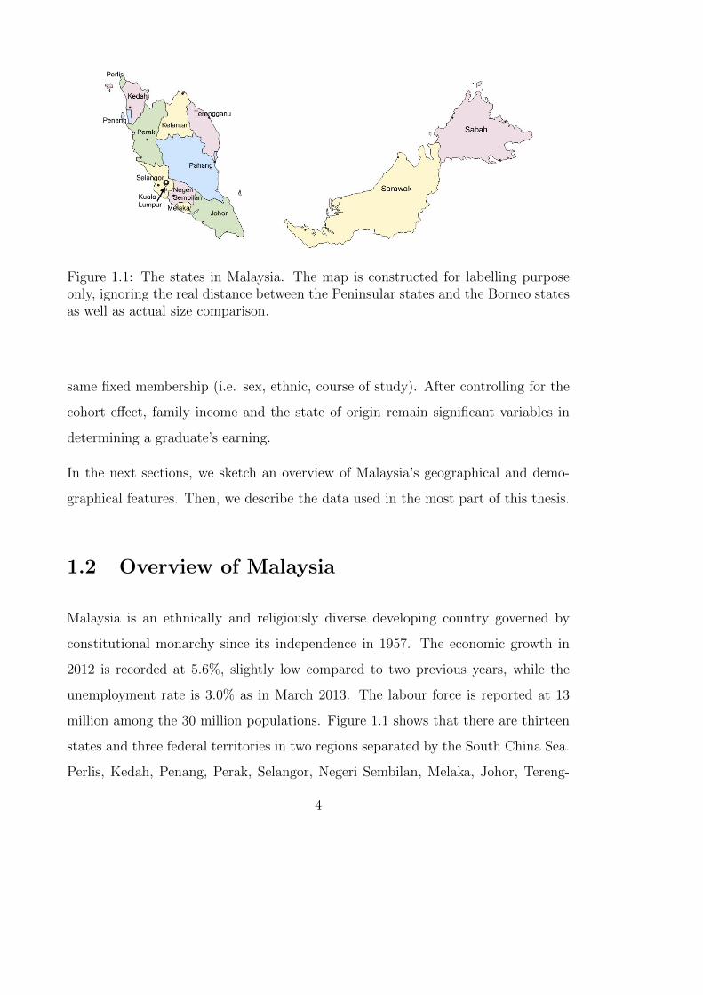
Figure 1.1: The states in Malaysia. The map is constructed for labelling purposeonly, ignoring the real distance between the Peninsular states and the Borneo statesas well as actual size comparison.
same fixed membership (i.e. sex, ethnic, course of study). After controlling for the
cohort effect, family income and the state of origin remain significant variables in
determining a graduate’s earning.
In the next sections, we sketch an overview of Malaysia’s geographical and demo-
graphical features. Then, we describe the data used in the most part of this thesis.
1.2 Overview of Malaysia
Malaysia is an ethnically and religiously diverse developing country governed by
constitutional monarchy since its independence in 1957. The economic growth in
2012 is recorded at 5.6%, slightly low compared to two previous years, while the
unemployment rate is 3.0% as in March 2013. The labour force is reported at 13
million among the 30 million populations. Figure 1.1 shows that there are thirteen
states and three federal territories in two regions separated by the South China Sea.
Perlis, Kedah, Penang, Perak, Selangor, Negeri Sembilan, Melaka, Johor, Tereng-
4

ganu, Pahang, and Kelantan are the eleven states in the eastern side of the country
called the Peninsular Malaysia, where Kelantan, Perlis, Kedah and Perak share bor-
der with Thailand. Kuala Lumpur is located in the middle of Selangor. On the
Borneo island there are two states: Sabah and Sarawak, and a federal territory
Wilayah Persekutuan Labuan (Labuan). The services and the manufacturing sec-
tors remained as the key engine to the growth. The performance of Selangor, Kuala
Lumpur, Johor, Sarawak and Penang contributed 75% to the national momentum.
The states of Selangor and Kuala Lumpur both dominate a quarter of total percent-
age share of services sector each, followed by Johor, Sarawak, Perak, and Penang.
Selangor on the other hand dominates manufacturing sector (0.297 of total), fol-
lowed by Pulau Pinang (0.136 of total) and Johor (0.126 of total). Agriculture is
more dominant in the states of Sabah, Johor and Sarawak. Labuan, Kuala Lumpur,
Selangor, Pahang and Perak are the top five states in economic growth. Table 1.1
shows the gross domestic product per capita for each state in 2012 and 2013.
Population distribution by state in Table 1.2 indicated that Selangor is the most
populous state (5.46 million), followed by Johor (3.35 million) and Sabah (3.21
million). The population share of these states to the total population of Malaysia
was 42.4 per cent. The least populated states were Putrajaya (72,413) and Labuan
(86,908). Population density of Malaysia is at 86 persons per square kilometre in
2010 compared with 71 persons in 2000. Unlike the population distribution, the
population density revealed a different picture. Selangor being the most populous
state was only ranked fifth in terms of population density with 674 persons per
square kilometre. Among the most densely populated states were Kuala Lumpur
(6,891 persons per kilometre), Penang (1,490 persons per kilometre) and Putrajaya
(1,478 persons per kilometre). The World Bank reported the urban population in
Malaysia was last measured at 75 per cent in 2015 while differences exist across
5
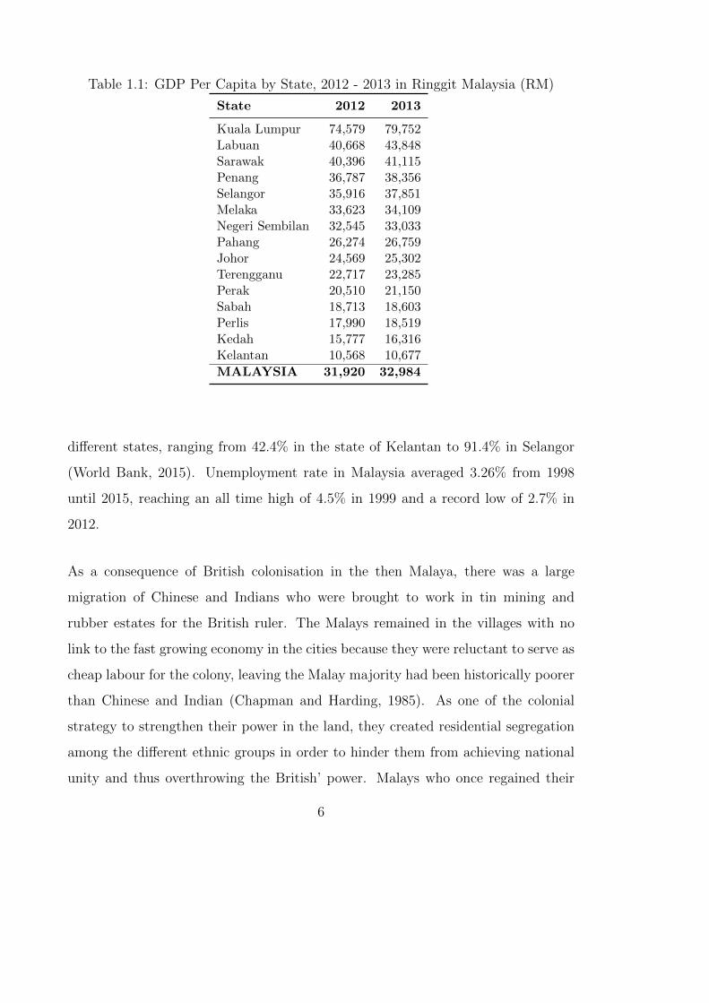
Table 1.1: GDP Per Capita by State, 2012 - 2013 in Ringgit Malaysia (RM)
State 2012 2013
Kuala Lumpur 74,579 79,752Labuan 40,668 43,848Sarawak 40,396 41,115Penang 36,787 38,356Selangor 35,916 37,851Melaka 33,623 34,109Negeri Sembilan 32,545 33,033Pahang 26,274 26,759Johor 24,569 25,302Terengganu 22,717 23,285Perak 20,510 21,150Sabah 18,713 18,603Perlis 17,990 18,519Kedah 15,777 16,316Kelantan 10,568 10,677
MALAYSIA 31,920 32,984
different states, ranging from 42.4% in the state of Kelantan to 91.4% in Selangor
(World Bank, 2015). Unemployment rate in Malaysia averaged 3.26% from 1998
until 2015, reaching an all time high of 4.5% in 1999 and a record low of 2.7% in
2012.
As a consequence of British colonisation in the then Malaya, there was a large
migration of Chinese and Indians who were brought to work in tin mining and
rubber estates for the British ruler. The Malays remained in the villages with no
link to the fast growing economy in the cities because they were reluctant to serve as
cheap labour for the colony, leaving the Malay majority had been historically poorer
than Chinese and Indian (Chapman and Harding, 1985). As one of the colonial
strategy to strengthen their power in the land, they created residential segregation
among the different ethnic groups in order to hinder them from achieving national
unity and thus overthrowing the British’ power. Malays who once regained their
6

Table 1.2: Urbanisation and population distribution by state
State Urbanisation % State Population (in millions)
Putrajaya 100 Selangor 5.46Kuala Lumpur 100 Johor 3.35Selangor 91.4 Sabah 3.21Penang 90.8 Sarawak 2.47Melaka 86.5 Perak 2.35Labuan 82.3 Kuala Lumpur 1.67Johor 71.9 Penang 1.56Perak 69.7 Kelantan 1.54Negeri Sembilan 66.5 Pahang 1.5Kedah 64.6 Terengganu 1.04Terengganu 59.1 Negeri Sembilan 1.02Sabah 54 Melaka 0.82Sarawak 53.8 Perlis 0.23Perlis 51.4 Labuan 0.09Pahang 50.5Kelantan 42.4
power in 1957 had to compete with Chinese and Indians who had a head start
in the economy. Government official has tried to correct this since 1971 through
the New Economic Policy (NEP) of affirmative action by giving Malays priority in
university scholarships and governmental jobs. Although since 1971 Malays have
benefited from positive discrimination in business, education, and civil services,
ethnic Chinese continue to hold economic power and are the wealthiest community.
The consequence of the NEP policy and its New Economic Model have also lead to
brain drain, particularly among the educated ethnic Chinese and Indian who leave
Malaysia to seek fairer treatment elsewhere. In 2010 the World Bank reported that
these groups have now made up the majority of the Malaysian diaspora; estimated
to be around 1.4 million people (World Bank, 2011).
In the next section, we discuss educational system in Malaysia highlighting on higher
education.
7

1.3 Educational system in Malaysia
Malaysian education pattern has typically been eleven years of schooling followed
by a transition period of pre-university educations before entering higher education
to a first degree. The eleven years of schooling is divided in three parts: primary
school from age seven at Standard 1 to age twelve at Standard 6, where students
sit for the Primary School Achievement Test at the end of Standard 6; followed by
lower secondary school from age 13 at Form 1 to age 15 at Form 3, where students
sit for Lower Secondary Assessment; and finally two years of higher secondary which
ends at Form 5, where students sit for Malaysian Education Certificate equivalent
of O-Level.
Pre-university education is offered by matriculation (commonly known to be offered
to top students, one year preparation for university education), or taking a two-years
Sixth Form, or Diploma. Higher education is offered by either public university, pri-
vate university, or international universities abroad. Application for entering public
university is centralised by the university intake unit who locate the students in any
of the preferred course of study and/or university of choice based on availability and
students’ ability. Top universities usually have the privilege of choosing the highest
ranking students arranged by the university intake unit, while less-fortunate stu-
dents will have to be located to any available courses of studies and/or universities
that still have the availability. Students may choose to accept the offer, or choose
another institutions such as private universities or studying abroad. Commonly stu-
dents coming from low to middle income families will tend to accept the offer by
studying at a public university due to lower costs.
Table 1.3 shows the number of university graduates for all levels of education pro-
duces in the year 2013. Figure 1.2 shows the composition of graduates within each
8

higher learning institution in 2013.
Table 1.3: Total number of graduates produced by Malaysia higher learning insti-tutions in 2013 based on awarded certificates.
Awarded certificate Number of graduates
Diploma 99292Professional 343First Degree 96745Master’s Degree 15550PhD 1819Certificates 7182Total 220931
9

Total220,931
Other HEI33,368
Others166
IPMARA786
KBS22
ILTJM101
CommunityColleges
5,350
Polytechnic26,943
Private73,365
Others19,435
Collegeuniversities
15,292
Universities38,638
Publicuniversities
114,198
Figure 1.2: Total number of graduates produced by participating higher educationinstitutions in Malaysia including all levels of studies for the year 2013.
10

1.4 Description of the Graduate Tracer Study data.
In 2002 with the collaboration of the Economic Planning Unit, the Prime Minister’s
Department, the Public Higher Education Institutions (Public HEI), the Private
Higher Education Institutions (Private HEI), and Polytechnics, the government of
Malaysia has introduced a university exit survey known locally as the Graduate
Tracer Study. The respondents involved are graduates who have finished study
and are qualified to receive certification. The study is conducted every year during
convocation involving all public universities and almost all private higher educations.
The system is open two to three weeks before convocation and closes one week after
the convocation. Starting from 2006 the questionnaire were made online to reduce
operational cost and data storage while increasing universities’ participation rate.
The main objective is to study graduate employability and marketability. The survey
covers all graduates of all levels - Diploma, first degree, and post-graduate levels.
The response rate for nine years of online operation averages around 81.51%, in-
creasing on yearly basis due to the committee’s affirmative action and institutions’
benefiting from the report outcome. The most recent data available when this thesis
starts is the 2013 survey capturing 220,931 graduates of all levels of studies, 96,745
of those are first degree graduates. This study focuses on first degree graduates
employment and earnings, the term ‘graduate’ henceforth refer to the first degree
graduates.
The graduates were asked about their socio-economic background (age, marital sta-
tus, place of origin, family income, disability status; academic and skill competen-
cies; educational experience (type of university, name of university, courses, field of
study, industrial training status, financial assistance or funding, and mode of study);
job information (employment status, reasons for unemployed, type of organisation,
11

income, industry, part time job, job level, address of workplace); and other rating
questionnaire: retrospective questions on the satisfaction on university facilities,
teaching environments and quality.
The age distribution of the graduates ranges from 19 to 69 with positive skew and
clustered between the common age of between 22 and 27. Entry to a first degree
requires graduates to pass either one of these after their O level certificate at the
age of 17: a one-year matriculation, two-years A level, or a three-years Diploma.
Some graduates may have taken up the advance class for the bright student which
allow them to skip one year of schooling (e.g. from Year 3 straight to Year 5).
Theoretically, the earliest age for first degree graduation is 20, and the occurrence
of one respondent with age 19 might be caused by at the date of convocation the
respondent has not reached the age of 20. However, in order for this analysis to
be representative of fresh graduates, the age has been filtered so the focus is on
graduates between the age of 22 to 27.
Graduates with a disability were also filtered out for they may have different at-
tributes of labour market. Most of the foreign students went back to their home
country and thus were removed. The academic achievement for most graduates was
recorded in a cumulative grade point average (CGPA) ranging from 0.00 to highest
score at 4.00. The passing mark is at 2.00 needed for graduation. Some Medical and
Dentistry students in several institutions do not have CGPA measure, instead, they
were only labeled as “passed”. Obviously, all of graduating Medical and Dentistry
graduates passed their studies. Analysis involving CGPA for these graduates may be
seriously biased because the majority of them have a missing value on CGPA. Con-
sidering Medical and Dentistry graduates have the toughest entry level grade where
only the brightest was accepted into the course, and the passing mark is exception-
ally intensive, then it is natural to impute the missing CGPA with 4.00. It is also
12
evident that Medical and Dentistry graduates’ employment rate is the highest com-
pared to graduates from other fields. Their earning is also significantly higher. The
measurement of English language ability is observed through the graduate’s score in
a national standardised English proficiency test, the Malaysian University English
Test (MUET) which was taken prior to admission. Even though the graduates may
have spent several years in education but their MUET score remains a significant
measure of their English language proficiency until graduation (see Rethinasamy
and Chuah (2011)).
A different institution may use a different name for their offered courses of studies,
and these have been reduced to 24 major courses of study as in Table 1.4. The details
of all the variables being used are shown in Table 1.4 with their descriptive statistics
in Table 1.5. Graduates income is observed in monthly income in eight incremental
level - the lowest below RM500 and the highest is more than RM5,000, where the
graduate’s entry level is averaged at RM2,000. Almost half of the graduates were
employed by the private local corporation and a quarter was employed by the private
multinational corporation. 15% of the graduates were employed in the public sector.
Another 11% were self-employed in their business or freelancing activities. The
majority of the employed graduates work in professional jobs, followed by clerical
support, and sales and services. Half of the employed graduates were employed
in permanent job level. The largest economic sector among the graduates was in
other services and professional, scientific, and technical occupation type, followed
by manufacturing, education, and construction.
13

Table 1.4: Data description - the Graduate Tracer Study
Variable Description
Ability
cgpa Grade Point Cumulative Averageenglish Malaysian University English Score (MUET)muet1 Band 1 (lowest)muet2 Band 2muet3 Band 3muet4 Band 4muet5 Band 5muet6 Band 6 (highest)
Education
publicuni Public universityprivateuni Private universitycourses courses of studycourses1 Lawcourses2 Arts / Social Sciencecourses3 Transportcourses4 Administrationcourses5 Managementcourses6 Economycourses7 Accountancycourses8 Marketingcourses9 Financecourses10 Journalismcourses11 Islamiccourses12 Food/hospitalitycourses13 Artscourses14 Pure sciencecourses15 Applied sciencecourses16 Pharmacycourses17 Medicalcourses18 Dentistrycourses19 Nursecourses20 Environmentcourses21 Sportscourses22 Engineeringcourses23 Computer Sciencecourses24 Education
Socio-economic
male Dummy, 1 if male
Continued on next page
14

Table 1.4: Data description - the Graduate Tracer Study
Table 1.4 – continued from previous page
Variable Description
age Age of respondentrace Main ethnic groupmalay 1 Malaychinese 2 Chineseothers 3 Indian and othersfaminc Family incomefaminc1 1 Less than RM500faminc2 2 Between RM501 to RM1000faminc3 3 Between RM1001 to RM1500faminc4 4 Between RM1501 to RM2000faminc5 5 Between RM2001 to RM2500faminc6 6 Between RM2501 to RM3000faminc7 7 Between RM3001 to RM5000faminc8 8 More than RM5000
Job related variables
employment 1 Full time employment, 2 Part time employment, 3 Continuestudy, 4 Unemployed.
joblev Job leveljlev1 1 Permanentjlev2 2 Contractjlev3 3 Temporaryjlev4 4 Self-employedjgroup Job groupjgroup1 Managerjgroup2 Professionaljgroup3 Technicianjgroup4 Admin supportjgroup5 Salesjgroup6 Prof. Agri.jgroup7 Commercejgroup8 Machineryjgroup9 Basicpublic Dummy, 1 if individual is hired in public sector
industry Industryindustry1 1 Agriculture, forestry, and fishingindustry2 2 Mining and quarryindustry3 3 Manufacturingindustry4 4 Electric, gas, steam, and air-conditioning supplies
Continued on next page
15

Table 1.4: Data description - the Graduate Tracer Study
Table 1.4 – continued from previous page
Variable Description
industry5 5 Water supply, sewerage, waste management, and related ac-tivities
industry6 6 Constructionindustry7 7 Wholesale and retail trade, repair of motor vehiclesindustry8 8 Transport and storageindustry9 9 Accommodation and food services activitiesindustry10 10 Information and communicationindustry11 11 Finance and insuranceindustry12 12 Real estateindustry13 13 Professional, scientific and technicalindustry14 14 Administrative and support servicesindustry15 15 Public administration and defense, compulsory social secu-
rityindustry16 16 Educationindustry17 17 Health and social workindustry18 18 Arts, entertainment, and recreationindustry19 19 Other servicesindustry20 20 Household / domestic personnelindustry21 21 Corporate and organization outside the regiongradinc Graduates’ monthly incomegradinc1 1 Less than RM500gradinc2 2 Between RM501 to RM1000gradinc3 3 Between RM1001 to RM1500gradinc4 4 Between RM1501 to RM2000gradinc5 5 Between RM2001 to RM2500gradinc6 6 Between RM2501 to RM3000gradinc7 7 Between RM3001 to RM5000gradinc8 8 More than RM5000
16

Tab
le1.5
:D
escr
ipti
ve
stati
stic
s-
the
Gra
du
ate
Tra
cer
Stu
dy.
Item
Vari
ab
leN
Per
centI
tem
Vari
ab
leN
Per
cent
Fir
std
esti
nat
ion
Fu
llti
me
job
29,9
54
39%
Job
leve
lP
erm
an
ent
17,6
48
49%
Part
tim
ejo
b5,7
14
8%
Contr
act
8,8
77
25%
Conti
nu
est
ud
y5,8
75
8%
Tem
pora
ry8,0
86
23%
Un
emp
loye
d34,3
26
45%
Sel
f-em
plo
yed
/fa
mil
y1,0
57
3%
Aca
dem
icsc
ore
CG
PA
3.1
6Job
Man
ager
2,3
38
7%
MU
ET
scor
eB
an
d1
4,3
67
7%
gro
up
Pro
fess
ion
al
18,8
17
53%
Ban
d2
20,5
77
33%
Tec
hn
icia
n2,3
40
7%
Ban
d3
26,0
46
41%
Ad
min
sup
port
5,3
83
15%
Ban
d4
9,9
92
16%
Sale
s4,5
84
13%
Ban
d5
1,8
37
3%
Pro
f.A
gri
.164
0.5
%B
an
d6
93
0%
Com
mer
ce500
1%
Un
iver
sity
Pub
lic
58,3
56
77%
Mach
iner
y138
0.4
%P
riva
te17,5
14
23%
Basi
c1,4
04
4%
Cou
rses
Law
1,5
62
2%
Sec
tor
Pu
bli
c4758
13%
Art
s/S
ocS
c4,0
60
5%
Pri
vate
30911
87%
Tra
nsp
ort
249
0.3
%In
du
stry
Agri
cult
ure
/F
ore
stry
/F
ish
ing
553
2%
Ad
min
istr
ati
on
4,4
20
6%
Min
ing/Q
uarr
y205
1%
Man
agem
ent
7,2
33
10%
Manu
fact
uri
ng
3,6
99
10%
Eco
nom
y1,6
20
2%
Ele
ctri
c/G
as/
Ste
am
708
2%
Acc
ou
nta
ncy
4,4
92
6%
Wate
r/S
ewer
age
157
0%
Mark
etin
g1,4
06
2%
Con
stru
ctio
n3,1
55
9%
Fin
an
ce3,4
68
5%
Wh
ole
sale
1,4
13
4%
Jou
rnali
sm1,7
99
2%
Tra
nsp
ort
/S
tora
ge
768
2%
Isla
mic
995
1%
Food
/A
ccom
.1,4
02
4%
Food
/h
osp
itali
ty1,4
04
2%
IT/C
om
m.
2,6
30
7%
Art
s1,9
05
3%
Fin
an
ce/In
sura
nce
3,0
94
9%
Pu
resc
ien
ce1,2
54
2%
Rea
les
tate
514
1%
Ap
pli
edsc
ien
ce4,9
14
6%
Sci
enti
fic/
Tec
hn
ical
4,7
84
13%
Ph
arm
acy
820
1%
Ad
min
/S
up
port
1,3
54
4%
Med
ical
2,5
38
3%
Def
ence
239
1%
Den
tist
ry365
0.5
%E
du
cati
on
3,5
13
10%
Conti
nu
edon
nex
tp
age
17

Tab
le1.5
:D
escr
ipti
ve
stati
stic
s-
the
Gra
du
ate
Tra
cer
Stu
dy.
Table
1.5
–continued
from
pre
viouspage
Item
Vari
ab
leN
Per
centI
tem
Vari
ab
leN
Per
cent
Nu
rse
1,2
91
2%
Soci
al
work
1,3
69
4%
Envir
on
men
t1,5
18
2%
Art
s694
2%
Sp
ort
s317
0.4
%O
ther
serv
ices
4,6
56
13%
En
gin
eeri
ng
17,4
78
23%
Dom
esti
c658
2%
Com
pS
ci5,2
29
7%
Extr
a-t
erri
tory
103
0.3
%E
du
cati
on
5,5
33
7%
Gra
du
ate
<R
M500
1,5
40
4%
SE
S∗
Male
27,3
80
36%
inco
me
RM
501
-R
M1000
5,5
23
15%
Fem
ale
48,4
90
64%
RM
1001
-R
M1500
5,8
31
16%
Mala
y51,9
18
68%
RM
1500
-R
M2000
7,8
37
22%
Ch
ines
e16,2
98
21%
RM
2001
-R
M2500
7,4
45
21%
Oth
eret
hn
ic7,6
54
10%
RM
2501
-R
M3000
4,5
33
13%
Age
23.7
RM
3000
-R
M5000
2,6
64
7%
Fam
ily
inco
me
<R
M500
5,5
11
7%
>R
M5000
295
1%
RM
501
-R
M1000
13,5
73
18%
RM
1001
-R
M1500
11,5
17
15%
RM
1500
-R
M2000
9,7
16
13%
RM
2001
-R
M2500
7,4
25
10%
RM
2501
-R
M3000
9,7
13
13%
RM
3000
-R
M5000
10,5
98
14%
>R
M5000
7,8
17
10%
SE
S∗
=so
cial
econ
omic
statu
s.
18

Chapter 2
Graduate’s first destination choice
and employment.
2.1 Introduction.
Graduate experience in embarking into labour force in recent times is more varied
and less standardised compared to the previous decades. Transition from university
to labour market is prolonged, and graduates take longer time to establish them-
selves into the labour market which cause some to experience repeated period of
unemployment or attached to marginal form of employment. Some graduates may
return to education or training, while others take the time out for leisure.
This chapter is set to answer several questions on the graduates transition from ed-
ucation to work. First, we examine four possible graduates’ first destinations after
study - they either get a full time employment, part time employment, continue to
study, or remain unemployed at the time the survey data was gathered. Second, we
examine occupational choices among graduates who are employed. We investigate
19
the determinants that are associated with different job levels (i.e. permanent, con-
tract, temporary, or self-employment). Third, we explain gender differences within
each of the first destination choice. We also investigate gender differences in differ-
ent occupational types. Women’s lower participation in superior occupational types
can be explained by their preferences in courses that have less demand in the labour
market. In order to investigate if attaining the same qualification with men would
reduce women’s performance, we compute gender differences in different employ-
ment outcome within the same courses. All else equal, we still found that women
who possess the same qualification as men are under-represented in the superior
occupational types compared to men.
Generally, we found that higher academic performance, better English proficiency,
higher family income, the choice of courses of study largely influenced graduate’s
better employment outcomes. Graduates with better characteristics as mentioned,
are more successful in gaining full time employment, permanent job level, and profes-
sional job category. However women are found to be consistently under-represented
in superior occupational types - some are largely due to their preference in less at-
tractive courses, some are due to unmeasured observations that may signify discrim-
ination or taste. Nonetheless, our result is consistent with the previous literatures
in the country who found that women are less preferred in Managerial job positions
and instead segregated into Administration Support jobs. Further investigation on
taste would be helpful to disentangle the reason of women segregation into lower
occupational status.
This paper contributes to the literature in terms of the use of a wider spectrum of
analysis that cover large categories of occupational types which is not limited to a
binary employed-unemployed category. The detailed categorisation of occupational
types allow us to investigate uniquely the impact of graduate’s achievement, char-
20
acteristics, and experiences that influence their settlement into the labour market.
The innovative aspect of this paper is when we disentangle the gender differences
within each course of study to investigate if women with the same qualification as
men would have similar employment opportunity.
Besides contributing to the literature on Malaysian graduate employment, our re-
sults may inform the policy of university admission especially related to the Malays
and women. Malay and women’s inferior employment outcomes are due to their
choice of less desired courses, where the sorting into such courses originated from
their lower academic performance at schools. One way to reduce unemployment
among these groups might be to reduce the intake of courses that are not demanded
by the labour market and instead increase the participation into STEM1 courses. If
a student are not qualified to enter university and take up such courses, then voca-
tional training must be promoted. Courses that are less demanded should not be
entirely banished (due to their contribution towards social benefits and knowledge
creation), but the admission into such courses should be limited in order to reduce
the incidence of over-education where graduate receive the wrong signal and they
invest in education that do not help them in their career.
The chapter is arranged as follows. In section 2.2 we discussed the underlying
theory behind graduate employment. Section 2.3 describes the sample data used in
this study. Section 2.4 introduces the econometric framework to analyse graduates
employment outcomes. The results are discussed in section 2.5 and finally section 2.6
concludes the findings.
1Science, Technology, Engineering, and Mathematics
21
2.2 Literature review.
Graduate’s transition from education to work increasingly gains worldwide attention
due to the expansion of higher education institutions and proliferation of tertiary
education enrolment across the globe. Worldwide studies on graduate labour market
such as the Malaysian’s Graduate Tracer Study, the United Kingdom’s Higher Ed-
ucation Data and Analysis (UK HESA), the European’s Careers after Graduation
- an European Research Survey (CHEERS), Canada’s National Graduate Survey
(NGS), and various reports from universities and survey institutions are established
to conduct research on the process of transitioning from university to work. They
collect data on graduate characteristics, educational choices, achievements, and ex-
periences, and information on first destination choice after study. The studies in-
volved identifying the determinants of graduates employability and earnings, the
effect of migration, the incidence of over-education, and the job search duration to
gain employment after finished study, and the differences between countries (Muller
and Gangl, 2003).
Technological progress in the current times require high skilled workers to fulfil
the jobs - which can be achieved through the massification of higher education.
Education enhances individuals productivity and reduces social inequality among
traditionally disadvantaged group and minimise social disparity. In the emergence of
knowledge economy the expansion of higher learning institutions supply high skilled
workers into the labour market but it also lead to more diversified composition
of graduates which include individuals who would not have attended university
by the previous standard. The side effect of higher education expansion may has
detrimental consequences for graduate labour market outcomes. High participation
rate would lead to credential inflation in which case if there are more highly educated
graduates than the labour market can absorb, the labour market value of credentials
22
will decline. In this case, some individual would be pushed downward to accept jobs
that require less educational level than they acquired leading to over-education or
under-employment.
Achieving a degree has become a less distinguishing mark among employers. With-
out parallel improvement in the creation of employment opportunities, higher educa-
tion expansion would only lead to increased unemployment rate, increased education-
job mismatch, and increase over-education - all of which have detrimental conse-
quences to individual’s future employment (i.e. loss of human capital), health, and
motivation. Graduate jobs in current times are less defined and graduates are ex-
periencing employment in the marginal sectors, positions that were not considered
as suitable, more temporary and part time jobs, interrupted and uncommon ca-
reer path, and new type of self employment. Nonetheless, the demand for higher
education continues to grow seeing that as an escape route from low wage job.
Graduates leave educational system to obtain jobs that gives return for their invest-
ment in education in terms of monetary or non-pecuniary rewards. Their first job
would be a stepping stone for a better future. At the same time, employers looking
for applicants who are productive and least costly for the kind of work required
by the job. The matching model signify the overall outcome of such simultaneous
decisions by both parties that will be reflected in the social stratification.
Despite numerous efforts from the government and universities to increase graduate
participation in the labour market, the persistence of graduates’ high unemployment
rate lead to major concern which is reflected by the numerous studies on the tran-
sitional process. Due to rising unemployment many universities turn to more direct
form of active intervention into graduate labour market by introducing industrial
training and graduate training scheme aiming to increase employment participation
(see Pillai et. al. (2012)).
23

Courses of study are reported to have tremendous effect on employment prospects.
Highly technical courses such as Medical and Engineering improves individual’s em-
ployment prospect compared to graduates from Arts and Social Science studies - but
courses of study are also related to ability which then translate into better employ-
ment outcomes. One important aspect to give attention is that prospective students
should have been informed about what skills are rewarded in the labour market so
they can use the information in maximising their employment prospect (Assaad et.
al., 2014).
Unemployment can be the result of labour oversupply which lead to limited avail-
ability of jobs in the market but if there are constant unfulfilled vacant jobs in the
market, as in the case of Malaysia, it may signify a mismatch between graduate qual-
ification and skills required by the labour market. The general theme in Malaysian
graduate unemployment studies lingers around the same argument - Malaysian grad-
uates lack of skills necessary for employment (Rahmah, 2011), (Hanapi et. al., 2015),
(Nasrudin, 2004)2.
Another important aspect that take up most researches is graduates’ lack of ability to
communicate in English - this is especially true among rural female Malay graduates
2The general theme of researches of Malaysia graduate unemployment problem focuses on grad-uates lack of necessary skills for employment. (Rahmah, 2011) reports that graduates posses “un-suitable skill and qualification ... no good working performance”. From employers perspectiveof local graduates, Rahman et. al. suggest that “lecturers are lack of skill and higher educationcould not produce graduates with skills required in the labour market”. A report from the CentralBank in 2002 states that Malaysian graduates are “less skilled as compared to the internationalgraduates”. The skills mentioned include technical skills, problem-solving skills and communica-tion skills, especially in English language. (Hanapi et. al., 2015) found ten primary weaknesses ofMalaysian graduates are in the aspect of management, problem-solving, communication, leader-ship, creativity, critical thinking, proactive, self-confidence and interaction skills while (Nasrudin,2004) stated the eleven factors that lead to the unemployment problem among the graduates arethe relationship between capital intensive economy, a rapid increase of graduated workforce, lack ofthe relationship between educational institutions and the industry, lack of training for work prepa-ration, rapid increase of the population rate and rapid decrease of the mortality rate, educationaldevelopment, economic recession, quality of education, capability of graduates, and the graduatesskills and personalities.
24

(Ismail, 2011). Gender also plays a role, where women graduates are found to be
less employable (Nagaraj, 2014) and an argument is based on simply because there
are a lot more women graduates enrolled in tertiary education (Ismail, 2011). In
order to improve graduates employability, universities and industries introduced
several graduate employment programs (one example is MY Graduate Scheme).
Universities are also creating conducive environment for entrepreneurship (Ismail,
2011). Public universities implement industrial training at the end of study period,
where graduates are getting temporary unpaid placement in the industry which not
only give real life training but also saw many graduates absorbed into employment
at the end of internship period (Pillai et. al., 2012).
In their transition from education to settlement in employment, graduates use their
qualifications to secure jobs and towards future occupational and professional devel-
opment. Muller and Gangl (2003) states that initial job outcome is highly influential
to shape further development of work careers. Hence, graduates ability to settle
smoothly and successfully into labour market would minimise their experience of
unemployment and generate subsequent job progress. This implies that graduate’s
smooth transition also play important role towards shaping social stratification of
modern societies. At the same time, another social process take place with this
transition in terms of starting a household or family.
Does attending to different type of university affect graduates’ employment prospect?
Hilmer and Hilmer (2012) found evidence of earning premium among graduates
from better universities. Ability is hard to observe, but university credential pro-
vide “cheap sorting” to help employers identify better graduates (Hartog et. al.,
2010). Graduates from better universities also receive more invitation for interviews
(Drydakis, 2016).
Universities differ in terms of ranking, size, establishment type (public or private uni-
25

versities), and operational focus (research based versus teaching based) - all of which
may affect enrolment criteria and learning experiences. There are top tier research
based public universities in the country: University of Malaya, National University
of Malaysia, Universiti Putra Malaysia, and Science University of Malaysia, all of
which reside in the urban states. Not only they obtained larger share for research
expenditure from the government compared to all other public universities in the
country, they also have priority in choosing potential applicants during student in-
take through a central processing body (University Application Unit).
To cater for the need for tertiary education among its population without having
to rely on excessive spending from the government, under the Education Act 1996
Malaysia establishes more private universities which offer courses that are mostly
in demand. Private universities are found to offer professional courses with high
private benefit but low social benefit (Assaad et. al., 2014). A study from Malaysia
found that public universities spend more in library facilities, but private universities
spend more on computer and laboratory (Wilkinson and Yussof, 2005). Wilkinson
Yusof reported that: Information Technology courses are mainly offered by private
institutions; Medical and Dentistry are expensive investment but give good return
and hence are also offered by private universities; Economic and Business subjects
require short training and the syllabus are well established and they are also very
marketable so it is more likely to be offered by private universities; in contrast Ed-
ucation, Applied Sciences, and Pure Sciences are less likely to be offered due to the
lack of demand and they are already sufficiently provided by the public universities.
(Wilkinson and Yussof, 2005) also reported that Law are less likely to be offered
locally due to students getting law education abroad for international recognition.
As comparison to Wilkinson and Yussof (2005), our sample data show that Man-
agement are much more likely to be offered public universities; while Engineering,
Computer Sciences, Accountancy, Medical, and Administration are more likely to
26

be offered by private universities.
Yet, Teichler (2000) found that university effect is moderated by subject heterogene-
ity. Different courses of study might be associated with different level of ability, and
certain level of ability lead to successful employment. Certain courses (i.e. Med-
ical, Engineering, Dentistry) put high entry requirement and only the best school
leavers would be accepted into such courses. These courses are also associated with
high employment and more homogenous employment outcomes. Purcell and Pitcher
(1996) found that the subject of study is the single most important determinants
of the ease or difficulties to start a career while James et. al. (1989) found that the
effect of subject endogeneity towards earnings is larger than the university effect.
Many studies on graduate employment ascribed courses of study as the major deter-
minant on heterogeneity in employment outcomes (Dolton et. al., 1989), (Smith et.
al., 2000), (Robst and VanGilder, 2016), (Koshy et. al., 2016), (Chevalier, 2011).
Certain courses (i.e. Medical, Engineering, Dentistry) put tougher entry require-
ment and they are also associated with homogenous occupational types and higher
earning.3.
We further consider the influences of social and economic status towards employ-
ment. Women’s higher education attainment and lower fertility rate should imply
better employment prospects. However we found that women are under-represented
in full time employment, as well as permanent and professional jobs. The reason for
3This lead to the question of hierarchical effect of courses of study. In multilevel model frame-work, graduates are nested within a higher level organisation (i.e. courses of study) where thereis a possible relationship between the outcome variable and the higher level group. In universitysetting, graduates are clustered within a course of study, which are nested within a university. Sig-nificant higher level variance indicates variability in employment outcome which depends on thedifferences in the course of study (and university). If employment prospect between two individualstaking the same course at the same university are correlated with each other, the covariance inthe error terms between these two individuals would not equal to zero. We attempted to modelgraduate first destination choice and employment pattern using a multinomial multilevel modelbut the model never converge.
27

this inferior employment pattern among women can be explained by their choice in
course of study. Women graduates in our sample show significant tendency towards
courses that are associated with low employment prospects and lesser earnings.
Consistent with Hilmer and Hilmer (2012), we found that women are less likely to
choose Sciences and Engineering subjects. However in this thesis we do not cover
the reason for their preferences into such courses and we keep this for future re-
search. Gender segregations continue to exists even in developed countries where
women are found to concentrate on low paid and low productivity industries, part
time employment with poor promotional prospects and lower responsibility (Blau
and Kahn, 2000), even though women’s enrolment in tertiary education increases
and gender gap in receiving work related training reduces over the years (Green and
Zanchi, 1997). However, Wharton and Baron (1987) describes women’s preference
towards less demanding jobs in paradoxical way - that women choose these occu-
pations in order to balance between job and family (Glass, 1990), (Bender et. al.,
2005). In many Asian countries especially, women are still strongly committed to
family responsibility (Abdullah et. al., 2008). Women are less likely to be accepted
in male dominated organisational structure, instead, they are more likely to be of-
fered supporting positions (Ng and Chakrabarty, 2005). Osman and Shahiri (2014)
found that majority of Malaysian women are concentrated in low paying semi-skilled
jobs in the Manufacturing industry.
In the case of Malaysia, another important aspect that require attention is ethnic dif-
ferences in employment pattern. Unlike many other multiethnic countries, Malaysia
is unique in a sense that it is the ethnic majority that have lower employment rate
and earning compared to the other ethnic groups. The racial imbalance rooted from
the period of British colonisation’s divide and rule strategy. Economic sectors were
identified with race - the Chinese were located in the fast growing tin mining and
commerce, the Indians were placed in rubber plantations, and the Malays were lo-
28
cated in the rural areas where they concentrated in agriculture, and only a small
number of Indians and Malays served in the public sector (Zainudin and Zulkifly,
1982). Chinese and a few Malay aristocrats and Indians were more privileged to
attend schools that were available in the cities - leaving a large number of Malays
and Indians either uneducated or seriously lagged behind. The Bumiputeras avoided
jobs in the commercial industry (i.e. import, wholesale, retail) which are dominated
by the Chinese because it was difficult if not impossible to break into the strong net-
work (Salih and Young, 1989). Even after the implementation of the New Economic
Policy (NEP) to eradicate poverty and reduce ethnic disparity, the Malays continued
to be under-represented in industrial and modern sectors (Osman-Rani, 1982). More
recent study found that although Malay’s participation in professional and technical
jobs increases but they are more likely to be in the lower level occupations such as
teachers and nurse (Osman and Shahiri, 2014). Prolonged imbalance in ethnic share
in employment coupled with persistent earning inequality and poverty have led to a
tragic period of ethnic riot in 1969 (Gomez and Jomo, 1999) and continue to create
sparks in the current political arena.
Public university quota and the influence of family economic status become the basis
that lead to social stratification within public and private tertiary education institu-
tions in Malaysia. The ethnic group Chinese tend to be more successful in securing
jobs after graduating because of strong economic status among Chinese families. For
the same reason, they also tend to earn more than the other ethnic groups. Seeing
education as a solution to reduce social stratification, public universities regulates
a quota for student intake which favours the ethnic group Malay, and in particular
in UiTM, where the regulation require that the Malay to non-Malay quota is 9:1.
On the other hand, private universities usually have larger proportion of Chinese.
Universities like UniKL and UTM which focuses on highly technical courses have
higher proportion of male. These differences in the social demographic profiles of
29
graduates within a particular institution would have a great impact on aggregate
level analysis.
2.3 Data.
This section describes the sample used in this study. There are 35,688 employed
graduates out of the total 75,870 individuals observed. Table 2.1 shows the descrip-
tive statistics for our data. The employed have slightly higher academic achievement
(measured by CGPA) and better proficiency in English (measured by the MUET
score). The employed are also associated with coming from family with higher in-
come, slightly older, and originate from an urban state. Courses that are related to
the highest employment rate are: Medical, Accountancy, Computer Sciences, and
Administrations. At the opposite side, courses that are associated with the lowest
employment rate are: Pharmacy, Arts, and Pure Sciences.
Among the employed, the average job search duration is 2.1 months with almost
seven out of ten employed graduates obtained their job within the first two months.
Six out of ten gained employment in the urban states, while 30% stay at the state
where they attended university. 45% worked in local corporations, 24% in a multina-
tional corporation (MNC), 12% in public sector, and 10% in self employment. Half
of our employed graduates were offered a permanent job position, almost quarter
in contract job and another quarter in temporary jobs. 66% were in professional
job category which breaks down to 56% professionals, 6.5% managerial, and 6.5%
associated professional and technical jobs.
30
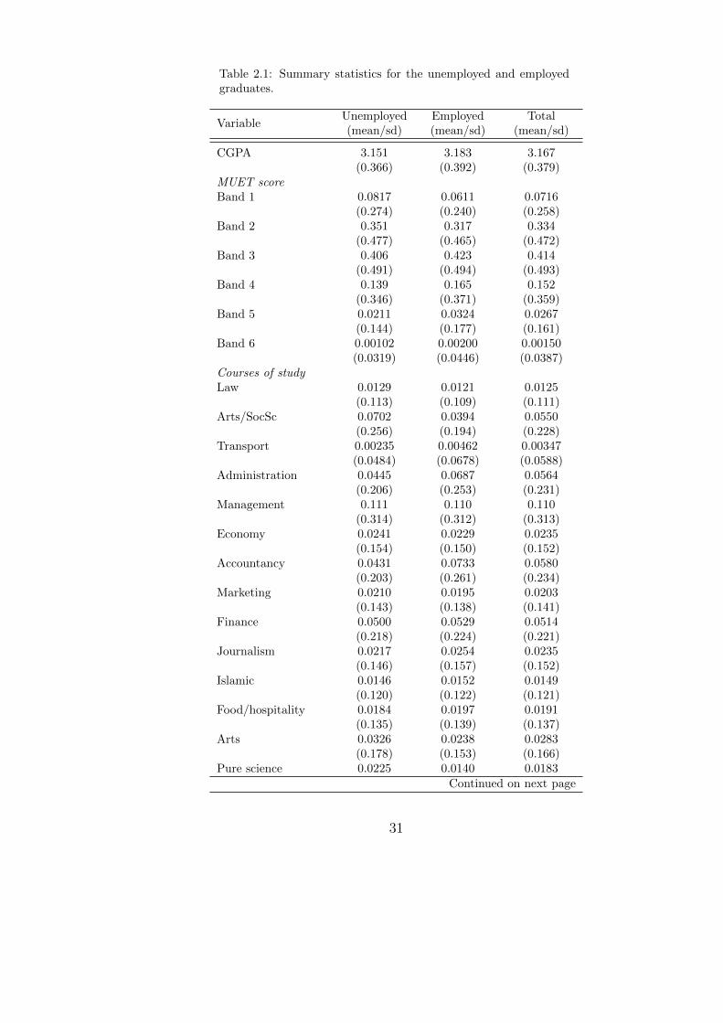
Table 2.1: Summary statistics for the unemployed and employedgraduates.
VariableUnemployed(mean/sd)
Employed(mean/sd)
Total(mean/sd)
CGPA 3.151 3.183 3.167(0.366) (0.392) (0.379)
MUET scoreBand 1 0.0817 0.0611 0.0716
(0.274) (0.240) (0.258)Band 2 0.351 0.317 0.334
(0.477) (0.465) (0.472)Band 3 0.406 0.423 0.414
(0.491) (0.494) (0.493)Band 4 0.139 0.165 0.152
(0.346) (0.371) (0.359)Band 5 0.0211 0.0324 0.0267
(0.144) (0.177) (0.161)Band 6 0.00102 0.00200 0.00150
(0.0319) (0.0446) (0.0387)Courses of studyLaw 0.0129 0.0121 0.0125
(0.113) (0.109) (0.111)Arts/SocSc 0.0702 0.0394 0.0550
(0.256) (0.194) (0.228)Transport 0.00235 0.00462 0.00347
(0.0484) (0.0678) (0.0588)Administration 0.0445 0.0687 0.0564
(0.206) (0.253) (0.231)Management 0.111 0.110 0.110
(0.314) (0.312) (0.313)Economy 0.0241 0.0229 0.0235
(0.154) (0.150) (0.152)Accountancy 0.0431 0.0733 0.0580
(0.203) (0.261) (0.234)Marketing 0.0210 0.0195 0.0203
(0.143) (0.138) (0.141)Finance 0.0500 0.0529 0.0514
(0.218) (0.224) (0.221)Journalism 0.0217 0.0254 0.0235
(0.146) (0.157) (0.152)Islamic 0.0146 0.0152 0.0149
(0.120) (0.122) (0.121)Food/hospitality 0.0184 0.0197 0.0191
(0.135) (0.139) (0.137)Arts 0.0326 0.0238 0.0283
(0.178) (0.153) (0.166)Pure science 0.0225 0.0140 0.0183
Continued on next page
31
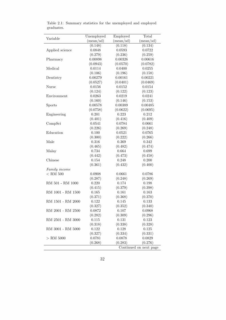
Table 2.1: Summary statistics for the unemployed and employedgraduates.
VariableUnemployed(mean/sd)
Employed(mean/sd)
Total(mean/sd)
(0.148) (0.118) (0.134)Applied science 0.0848 0.0593 0.0722
(0.279) (0.236) (0.259)Pharmacy 0.00898 0.00326 0.00616
(0.0943) (0.0570) (0.0782)Medical 0.0114 0.0400 0.0255
(0.106) (0.196) (0.158)Dentistry 0.00279 0.00161 0.00221
(0.0527) (0.0401) (0.0469)Nurse 0.0156 0.0152 0.0154
(0.124) (0.122) (0.123)Environment 0.0263 0.0219 0.0241
(0.160) (0.146) (0.153)Sports 0.00578 0.00389 0.00485
(0.0758) (0.0622) (0.0695)Engineering 0.201 0.223 0.212
(0.401) (0.416) (0.409)CompSci 0.0541 0.0784 0.0661
(0.226) (0.269) (0.248)Education 0.100 0.0521 0.0765
(0.300) (0.222) (0.266)Male 0.316 0.369 0.342
(0.465) (0.482) (0.474)Malay 0.734 0.664 0.699
(0.442) (0.473) (0.458)Chinese 0.154 0.248 0.200
(0.361) (0.432) (0.400)Family income< RM 500 0.0908 0.0661 0.0786
(0.287) (0.248) (0.269)RM 501 - RM 1000 0.220 0.174 0.198
(0.415) (0.379) (0.398)RM 1001 - RM 1500 0.165 0.161 0.163
(0.371) (0.368) (0.370)RM 1501 - RM 2000 0.122 0.145 0.133
(0.327) (0.352) (0.340)RM 2001 - RM 2500 0.0872 0.107 0.0968
(0.282) (0.309) (0.296)RM 2501 - RM 3000 0.115 0.131 0.123
(0.318) (0.338) (0.328)RM 3001 - RM 5000 0.122 0.128 0.125
(0.327) (0.334) (0.331)> RM 5000 0.0781 0.0878 0.0829
(0.268) (0.283) (0.276)Continued on next page
32

Table 2.1: Summary statistics for the unemployed and employedgraduates.
VariableUnemployed(mean/sd)
Employed(mean/sd)
Total(mean/sd)
Age 23.61 23.76 23.68(0.989) (0.995) (0.995)
Urban 0.244 0.380 0.311(0.429) (0.485) (0.463)
Observations 57972
mean coefficients; sd in parentheses
33

Table 2.2: Summary statistics of the job characteristics among theemployed graduates.
Job attributes (mean/sd) Job attributes (mean/sd)
Duration 2.117 Temporary 0.227(1.874) (0.419)
Urban (job) 0.601 Self-employed/family 0.0296(0.490) (0.170)
Unistay 0.307 Job group(0.461) Manager 0.0655
Sector (0.247)Government 0.119
(0.323) Professional 0.528(0.499)
Statutory body 0.0231(0.150) Technician 0.0656
(0.248)MNC 0.238
(0.426) Admin support 0.151(0.358)
Local corp 0.453(0.498) Sales 0.129
(0.335)Self-employed 0.101
(0.301) Prof. Agri. 0.00460(0.0677)
GLC 0.0314(0.174) Commerce 0.0140
(0.118)NGO 0.0204
(0.141) Machinery 0.00387Job level (0.0621)Permanent 0.495
(0.500) Basic 0.0394(0.194)
Contract 0.249(0.432)
Observations 35668
mean coefficients; sd in parentheses
34

Tab
le2.3
:E
mp
loym
ent
patt
ern
sby
un
iver
siti
es.
Un
iver
sity
N%
emp
loye
d%
urb
an
Un
ista
y∗
Un
iver
sity
N%
emplo
yed
%u
rban
Un
ista
y∗
Public
Universities
KU
HB
46
82%
59%
46%
UIA
M3,
068
59%
40%
14%
KU
IM15
21%
27%
7%
UK
M3,
366
45%
33%
15%
KU
IS252
66%
45%
22%
UM
1,95
055%
39%
14%
LE
LC
37
26%
68%
5%
UM
K51
942%
20%
5%
LIC
T6
67%
17%
0%
UM
P1,
383
44%
25%
3%
LU
C76
65%
46%
7%
UM
S3,
315
37%
10%
13%
LU
CT
198
15%
55%
5%
UM
T1,
629
40%
17%
8%
MA
HS
A43
69%
63%
7%
UN
IMA
S1,
986
42%
11%
16%
MM
MC
215
98%
45%
3%
UP
M3,
435
52%
37%
20%
MM
U1,9
16
60%
33%
13%
UP
NM
501
30%
29%
13%
MS
U392
76%
47%
31%
UP
SI
2,66
028%
11%
3%
MU
SM
566
51%
77%
22%
US
IM1,
211
57%
25%
7%
NE
C40
50%
70%
25%
US
M2,
872
39%
32%
12%
Nil
ai
U1
100%
0%
0%
UT
HM
1,73
754%
23%
9%
OU
M68
79%
32%
22%
UT
M2,
394
56%
24%
14%
SE
GiU
122
22%
83%
14%
UT
eM1,
436
55%
31%
7%
SW
INB
UR
NE
396
67%
2%
52%
UU
M4,
583
70%
25%
5%
TA
TiU
C89
22%
7%
15%
UiT
M18
,306
48%
39%
18%
TC
S18
25%
0%
17%
Un
iMA
P1,
458
32%
28%
2%
TU
C539
65%
64%
24%
Un
iSZ
A54
749%
18%
8%
TW
INT
EC
H117
75%
38%
29%
Tot
al58
,356
47%
26%
10%
UC
SI
U924
74%
64%
28%
Private
universities.
UN
IRA
ZA
K1,1
12
42%
24%
7%
AIM
ST
213
47%
39%
12%
UN
ISE
L801
65%
57%
31%
AM
U11
449%
39%
20%
UN
ITE
N1,4
71
64%
50%
26%
AP
U20
558%
80%
26%
UT
AR
3,1
76
56%
43%
17%
AU
CM
S66
7%
39%
0%
UT
P837
54%
35%
1%
CIT
YU
560%
60%
20%
Un
iKL
-BM
I341
62%
45%
30%
CU
SM
1100%
100%
100%
Un
iKL
-BiS
27
33%
52%
19%
HU
426
65%
81%
20%
Un
iKL
-IP
RO
M159
62%
52%
14%
IBS
10100%
0%
10%
Un
iKL
-ME
ST
EC
H76
26%
36%
11%
Conti
nu
edon
nex
tp
age
35
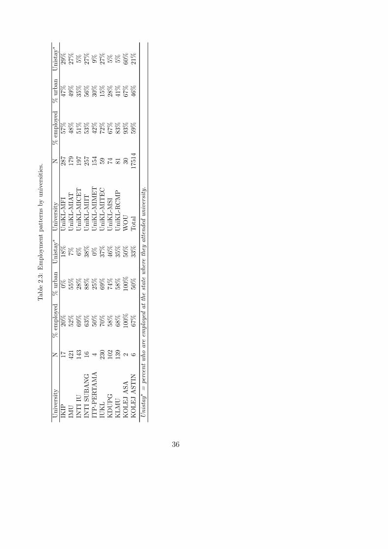
Tab
le2.3
:E
mp
loym
ent
patt
ern
sby
un
iver
siti
es.
Un
iver
sity
N%
emp
loye
d%
urb
an
Un
ista
y∗
Un
iver
sity
N%
emplo
yed
%u
rban
Un
ista
y∗
IKIP
1720%
0%
18%
Un
iKL
-MF
I287
57%
47%
29%
IMU
421
52%
55%
7%
Un
iKL
-MIA
T179
48%
49%
27%
INT
IIU
143
69%
28%
6%
Un
iKL
-MIC
ET
197
51%
35%
5%
INT
IS
UB
AN
G16
63%
88%
38%
Un
iKL
-MII
T257
53%
56%
27%
ITP
-PE
RT
AM
A4
50%
25%
0%
Un
iKL
-MIM
ET
154
42%
30%
9%
IUK
L23
070%
69%
37%
Un
iKL
-MIT
EC
59
72%
15%
27%
KD
UP
G10
258%
74%
46%
Un
iKL
-MS
I74
67%
28%
5%
KL
MU
139
68%
58%
35%
Un
iKL
-RC
MP
81
83%
41%
5%
KO
LE
JA
SA
2100%
100%
50%
WO
U30
93%
67%
60%
KO
LE
JA
ST
IN6
67%
50%
33%
Tota
l17514
59%
46%
21%
Unistay∗
=percen
twhoare
employedatthestate
wherethey
atten
ded
university.
36

Table 2.4: Employment patterns by courses of study.
Courses Percent employed Percent professional Percent permanent
Law 50% 90% 29%Arts/SocSc 40% 46% 30%Transport 67% 51% 51%Administration 60% 45% 56%Management 50% 41% 41%Economy 49% 38% 41%Accountancy 65% 80% 67%Marketing 50% 38% 54%Finance 51% 52% 45%Journalism 52% 63% 45%Islamic 51% 61% 12%Food/hospitality 55% 40% 54%Arts 42% 52% 26%Pure science 39% 59% 36%Applied science 42% 58% 45%Pharmacy 32% 70% 47%Medical 74% 94% 70%Dentistry 46% 95% 80%Nurse 49% 72% 45%Environment 44% 42% 39%Sports 40% 53% 34%Engineering 53% 86% 59%CompSci 58% 79% 53%Education 34% 61% 18%Total 51% 66% 49%
Table 2.3 shows employment patterns by university. For each participating public
and private university we report the average employment rate, the percentage of
urban graduates, and the percentage of those who obtained job at the state where
they attended university. The employment rates among different universities are
very mixed. Top three public universities (i.e. UM, UPM, UKM) have between 45%-
53% of employment rates. Public university in management has 70% employment
rate (UUM). The only international public university (UIAM) has 59% employment
rate. Employment rates among private universities are more mixed due to small
sample observed in some universities.
37

Table 2.4 shows employment pattern by courses of study. Medical, Dentistry, Law,
Engineering, Accountancy report high percentage of employment, professional job
(managerial, professional, technical) and higher percentage of permanent job posi-
tion.
38
2.4 Econometric framework.
2.4.1 Modelling graduate employment outcomes.
Consider the probabilistic outcomes in which graduates may find themselves in a
particular type of destination after study - they either choose to work in full time
employment, or work part time, or continue their education, or defer entry into
the labour market to a later date. A discrete response model can be modelled as
an ordered or nominal response. For an ordered response, we might assign each
graduate a particular type of the first destination where the response variable takes
the value of 3 for employed, 2 for further study, and 1 for unemployed. Each value
is ordered with the assumption that the lowest level (1: unemployed) has the lowest
rank, and the highest level is 3:employed. Indeed, we may also assign the value of
4 for full time employment, 3 for part time employment, 2 for further study, and 1
for unemployment with the basis that full time employment is at a higher rank than
part time employment.
For an unordered (or nominal) response, the value assigned to each outcome is
arbitrary in the sense that none of the destination is at the higher or lower rank
than the others. The individual outcome depends on individual characteristics rather
than the characteristics of the outcomes. A graduate may choose to obtain full time
employment right after study. For some, they may take a part time job in order
to gain experience to obtain a better job later on. Another graduate may choose
to further their study, and the rest are still actively looking for employment. On
the basis that the unemployed graduates are actively waiting for jobs, and those
who further study are not any better or worse than those who are working, we
decided to model graduate’s first destination as an unordered response. Implying
a graduate’s choice of the first destination after study is discrete (one of the four
39

mutually exclusive options) and unordered, the dependent variable can be denoted
by a categorical variable y which takes the value of
y =
1 if choose full time employment
2 if choose part time employment
3 if choose further study
4 if waiting for job
(2.1)
The potential outcomes y is then parametrised by conditioning vector X that in-
cludes a set of covariates such as individual academic achievement, English language
ability, and SES4 variables. A multinomial logit model can be used to model indi-
vidual choice among the discrete alternatives assuming each individual maximises
his or her utility. The probability that an individual i chooses option j ∈ {1, 2, 3, 4}
conditioning on covariates X is given by
Pr(y = j|X) = Pij =exp(X ′ijβ)∑Jj=1 exp(X ′ijβ)
(2.2)
The above response probability must sum to unity, hence to be able to identify the
model, one choice category must be set to become the base category. We choose
y = 4(unemployed) as the base category in this case, hence the remaining coeffi-
cients measure the relative change of each of the first destination outcome to the
unemployed category. The response probability now becomes
Pr(y = j|X) = Pij =exp(X ′ijβ
(j))
1 +∑J−1
j=1 exp(X ′ijβ(j))
(2.3)
4social and economic status
40
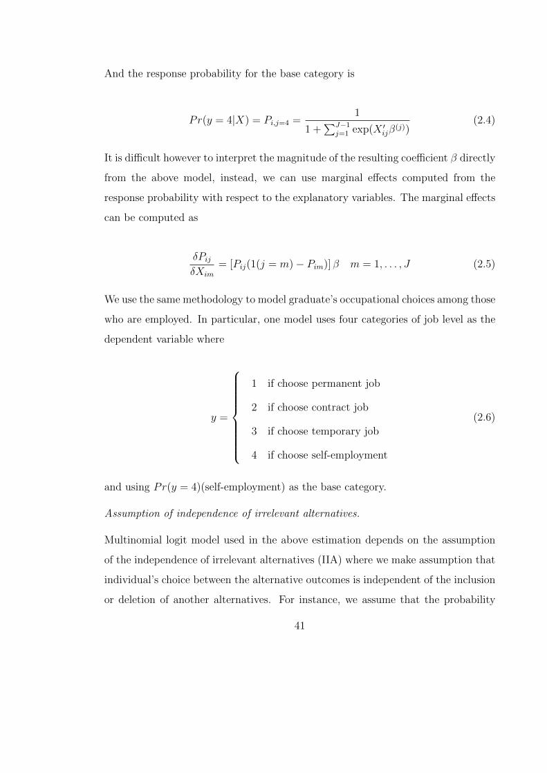
And the response probability for the base category is
Pr(y = 4|X) = Pi,j=4 =1
1 +∑J−1
j=1 exp(X ′ijβ(j))
(2.4)
It is difficult however to interpret the magnitude of the resulting coefficient β directly
from the above model, instead, we can use marginal effects computed from the
response probability with respect to the explanatory variables. The marginal effects
can be computed as
δPijδXim
= [Pij(1(j = m)− Pim)] β m = 1, . . . , J (2.5)
We use the same methodology to model graduate’s occupational choices among those
who are employed. In particular, one model uses four categories of job level as the
dependent variable where
y =
1 if choose permanent job
2 if choose contract job
3 if choose temporary job
4 if choose self-employment
(2.6)
and using Pr(y = 4)(self-employment) as the base category.
Assumption of independence of irrelevant alternatives.
Multinomial logit model used in the above estimation depends on the assumption
of the independence of irrelevant alternatives (IIA) where we make assumption that
individual’s choice between the alternative outcomes is independent of the inclusion
or deletion of another alternatives. For instance, we assume that the probability
41
of a graduate to choose self-employment is unaffected by the other occupational
choices available. This assumption can be tested using the Hausman-McFadden test
or the Small-Hsiao test (Hausman and McFadden, 1984),(Small and Hsiao, 1985).
However, Cheng and Long (2007) through their simulation experiments concluded
that the IIA is not satisfactory for applied analysis due to its dependency on the
data structure which give inconsistent results. Hence, we used Amemiya (1981)’s
suggestion by making sure that the alternatives are distinct in order to facilitate the
usability of a multinomial model.
2.4.2 Modelling gender differences in employment outcomes.
Consider the average employment rates between male and female graduates are
denoted by Ymale and Yfemale. The difference (Ymale) − (Yfemale) gives the mean
difference in the employment outcome between the two gender groups which can
be decomposed into two components: the characteristic effect that explains the
differences as caused by the differences in graduate’s attributes (e.g. differences in
the employment rate caused by the differences in academic achievement); and into
a component due to unmeasured or unobserved feature (Fairlie, 2005).
The decomposition technique is prominently used in various studies to explain the
differences in the mean level of a variable between any two groups (see Oaxaca(1979)
and Blinder(1979)). The original development of the technique uses linear method
but the development of non-linear methods allow for decomposition when the de-
pendent variable is in categorical form (see (Fairlie, 1999), (Fairlie, 2005), (Yun,
2004) and (Sinning et. al., 2008)).
The non-linear decomposition adapting (Fairlie, 1999) is given by
42

Ymale − Yfemale =
Nmale∑i=1
φ(Xi,maleβmale)
Nmale
−Nfemale∑i=1
φ(Xi,femaleβmale)
Nfemale
+
Nfemale∑i=1
φ(Xi,femaleβmale)
Nfemale
−Nfemale∑i=1
φ(Xi,femaleβfemale)
Nfemale
where Nmale and Nfemale are the sample sizes of male and female graduates, and
φ(.) is the average predicted probability. The first term of the equation decomposes
gender difference in the employment outcome due to the difference in the distribution
of explanatory variables which are included in the model. If male have superior
productive attributes and it translates into higher employment rate then this term
will capture the said effect. The second term of the equation bear the remaining
differences in (Ymale − Yfemale) into parts that cannot be measured by the existing
variables in the model.
We use the methodology in various settings. First, gender differences in employment
outcomes are computed within each of graduate’s first destination choice - full time
employment, part time employment, further study, or unemployed. Then, among the
employed graduates the gender differences are computed within each occupational
types.
To investigate if gender differences exist among women graduates who posses similar
qualification as men, we decompose gender differences in employment outcomes
within each course of study. We also computed gender differences in employment
outcome within each industry and region. Finally, the same methodology is being
used to decompose inter-ethnic differences in mean employment outcome within each
industry.
43
2.5 Empirical results.
This section begins by showing the estimation results of the determinants of gradu-
ate employment patterns. We first show the outcome of graduate’s first destination
during convocation which includes choosing to work in full time employment, part
time employment, continue study, or remain unemployed either by choice or be-
cause they defer entry to a later date. We proceed to describe who decides to take
permanent job, contract job, temporary job, or choose self-employment by charac-
terising the options depending on graduate’s characteristics. Subsequently, we anal-
yse gender differences in various employment outcomes. Part of women’s inferior
employment outcome can be based on their preferences for less attractive courses
that are associated with low employment rate and low paying jobs. We test the
underrepresentation of women graduates by studying the difference in employment
outcomes among women and men having similar qualifications. We also test for
gender differences within industry. The final part of this section discusses findings
in the employment outcome by different ethnic group.
2.5.1 Graduate’s first destination and job characteristics.
Table 2.5 presents the estimation results of graduate first destination outcomes.
The sample used in this analysis is 62,912 graduates. The marginal effects for
the multinomial logit model is presented separately for male and female graduates.
For each gender column, we report the effect of each explanatory variable based
in four choices of first destination outcomes: a graduate may choose to work full
time, part time, or choose to continue study, or remain unemployed. The set of
explanatory variables included in the model is: graduate’s academic achievement
(CGPA), English language ability (MUET score), course of study (Law as base
44
category), age, ethnic group, family income, and an urban dummy (=1 of a graduate
originated from Klang Valley or Penang).
Generally, we found that graduates from certain courses of study who did well
academically, with better English proficiency, and coming from higher family income
tend to have better employment outcomes. Graduates with better characteristics
as mentioned are more successful in gaining full time employment, permanent job
level, and professional job category. Detailed analysis is as follows.
The results show that an increase in academic achievement increases the probability
to participate in full time employment and decreases the probability to choose part
time employment or unemployment for both sexes. Employers look for applicants
who are productive and least costly for the kind of work required by the job, and
CGPA can be regarded as a human capital trait that demonstrate an individual’s
commitment and cognitive ability to perform challenging tasks and carrying out
responsibilities. The magnitude of CGPA effect for men is found to be larger than
women for full time employment showing that men’s academic achievement is re-
warded more than women. Another rationality for men’s more fortunate outcome
for their academic achievement is that men are more likely to posses qualification
in better courses, and their higher CGPA in those courses are rewarded more than
women’s higher CGPA in less attractive courses. On the other hand, part time em-
ployment and unemployment category are associated with lower CGPA. The impact
of lower CGPA towards part time employment is larger for women than for men.
However, we found that lower CGPA penalty affect men’s unemployment in higher
magnitude than women.
Getting a good grade from a good university may have a different effect than getting
a good grade from a lesser known university. Employers look for cheaply observed
attributes among job applicants and would prefer graduates from more prestigious
45
universities. Graduates who attended more selective institution went through tough
entry requirement and they possess aptitude and talent that made them successful
in their studies and subsequently in their jobs. After controlling for graduate’s
attributes we found that the university effect is moderated by the courses effect
and hence is not included in our model. We may, however, run another model by
including the university fixed effects.
Various local studies show the lack of English proficiency among the main deter-
minants towards graduate’s inability to secure a job. This is especially true among
Malay rural females. The effect of English language proficiency is measured by
MUET score. Our results show that its impact towards graduate’s first destination
outcome is found to be moderate compared to the effect of CGPA. MUET score does
not have any significant effect on men’s full time employment but it reduces part
time employment among men. On the other hand, moderate MUET score (Bands
3 - 4) increases female’s full time employment and choosing to further study, at the
same time reduces female’s part time employment.
We move on to discuss the effect of graduate’s characteristics. With each additional
year of age increases the probability of full time employment, and decreases the
probability for all other first destinations. Younger graduates took a faster route in
their education without any gaps during their study but older graduates may have
had temporary jobs during their study which help them to secure jobs as soon as
finishing studies, or they have the urge to get employed as soon as possible right
after finishing study.
Compared to the other ethnic group, Malay male coefficient for full time employment
is not significantly different but Malay women are less likely to obtain full time
employment as comparison to the other ethnic group. Instead, Malay men and
women are more likely to be in part time employment, additionally, Malay women
46
are more likely to further their education. Chinese men and women are more likely
to be in full time employment and less likely to choose other first destination choices.
We testify that parental income influences graduate’s first destination choice. Parental
income and residence are also related to ethnicity in which Malays mostly come from
rural areas with low family income. Higher family income increases the probabil-
ity of choosing full time employment while significantly decreases the probability of
unemployment. Higher family income provides means of network and more affluent
background to facilitate resources for an individual to attend interview and finding
a job, giving graduates from higher family income a competitive edge. Hence a
tertiary education may not be a perfect equaliser if social immobility in the country
persists. In overall, our finding shows that family income plays an important role in
shaping graduates employment.
Similarly, urban graduates are more likely to be in full time employment and less
likely to be unemployed. Living in an urban state may signify several features: first,
living in an urban state increases family income and family income significantly
influences graduate employment pattern. Second, the availability of jobs in the
urban state facilitates first job employment where urban graduates do not have
to migrate to find job elsewhere. Urban states offers more job availability with
competitive wage and access to high skilled jobs.
We further discuss the effect of courses of study. Certain courses are associated with
certain employment pattern as shown in Table 2.18 in the appendix. The effect of
courses of study using Law as the base category generally shows that women are
more advantageous in taking Business subjects5, Sciences subjects6, Engineering and
Computer Sciences.
5Administration, Management, Economy, Accountancy, Marketing, and Finance6Pure Science, Applied Science, Pharmacy, Medical, Dentistry, Nurse, Environment, and Sports.
47
Firstly, we discuss the pattern of full time employment. Business subjects increases
women’s probability for full time employment. The effect of Business studies is not
as advantageous for men in terms of significance and magnitude. Though the effect
of certain Business subjects such as Administration, Accountancy, and Finance are
positive and significant but lower in magnitude compared to women. The effect of
Food & Hospitality towards full time employment is more gainful for women than
for men. Applied Science increases women’s probability for full time employment
but decreases men’s probability for full time employment. The effect of Pharmacy
and Dentistry are lower for both sexes with larger magnitude among men. Medical,
Engineering, and Computer Science courses increase probability for full time em-
ployment, larger in magnitude for women. Considering women’s overall lower rate
of employment compared to men, this finding show that by taking highly technical
courses (i.e. Medical, Engineering, Computer Sciences) women may clearly improve
their employment prospects. Women’s choice for other Science subjects also found
to boost their full time employment prospect, while for men it is not significant.
We further discuss the patterns of part time employment. Using Law as the base
category, most other courses of study show significant positive coefficient towards
part time employment. Nonetheless, the magnitude of courses effect is much higher
among Education, Sports, Arts, Arts & Social Science, and Journalism for male and
female graduates. Female graduates who took Food & Hospitality, Pure Science,
and Environment are much more likely to choose part time employment, while male
graduates who took Nurse are much more likely to be in part time employment.
48

Tab
le2.5
:E
mp
loym
ent
ou
tcom
esam
on
ggra
du
ate
s.
Male
gra
du
ate
sF
emale
gra
du
ate
s(1
)(2
)(3
)(4
)(1
)(2
)(3
)(4
)F
ull
tim
eP
art
tim
eS
tud
yU
nem
plo
yed
Fu
llti
me
Part
tim
eS
tud
yU
nem
plo
yed
CG
PA
0.06
24∗∗
∗-0
.0192∗∗
∗0.0
340∗
∗∗-0
.0772∗∗
∗0.0
304∗
∗∗-0
.0227∗∗
∗0.0
364∗
∗∗-0
.0440∗∗
∗
Ban
d2
0.01
93
-0.0
104
0.0
0720
-0.0
161
0.0
141
0.0
0171
0.0
0341
-0.0
192
Ban
d3
0.02
58
-0.0
271∗
∗∗0.0
0936
-0.0
0807
0.0
306∗
∗-0
.0149∗∗
0.0
121∗
-0.0
279∗∗
Ban
d4
0.02
05
-0.0
374∗
∗∗0.0
112
0.0
0569
0.0
253∗
-0.0
204∗∗
0.0
142∗
-0.0
192
Ban
d5
-0.0
00296
-0.0
390∗∗
0.0
223
0.0
170
0.0
212
-0.0
128
0.0
233∗
-0.0
317
Ban
d6
0.08
09
0.0
0618
-0.0
596∗∗
∗-0
.0275
0.0
333
-0.0
532
-0.0
151
0.0
350
Age
0.04
45∗∗
∗-0
.00536∗
∗-0
.0111∗∗
∗-0
.0281∗∗
∗0.0
425∗
∗∗-0
.00529∗
∗∗-0
.00978∗
∗∗-0
.0274∗∗
∗
Mal
ay0.
00104
0.0
138∗
0.0
00635
-0.0
155
-0.0
222∗∗
0.0
146∗
∗0.0
121∗
-0.0
0442
Ch
ines
e0.
117∗∗
∗-0
.0225∗∗
-0.0
0402
-0.0
901∗∗
∗0.1
04∗∗
∗-0
.00905
0.0
132∗
-0.1
08∗
∗∗
RM
501
-R
M10
000.
0244
0.0
0153
0.0
0219
-0.0
281
0.0
245∗
∗0.0
0567
-0.0
0642
-0.0
237∗
RM
1001
-R
M15
000.
0575
∗∗∗
0.0
0113
-0.0
0292
-0.0
557∗
∗∗0.0
488∗
∗∗0.0
00139
-0.0
108
-0.0
381∗
∗∗
RM
1501
-R
M20
000.
0855
∗∗∗
-0.0
102
-0.0
118
-0.0
635∗∗
∗0.0
725∗
∗∗-0
.00118
-0.0
0848
-0.0
628∗∗
∗
RM
2001
-R
M25
000.
0756
∗∗∗
0.0
0459
-0.0
0223
-0.0
779∗
∗∗0.0
645∗
∗∗-0
.00472
-0.0
0959
-0.0
501∗∗
∗
RM
2501
-R
M30
000.
0838
∗∗∗
-0.0
0818
-0.0
0369
-0.0
720∗∗
∗0.0
494∗
∗∗-0
.00287
-0.0
0488
-0.0
417∗∗
∗
RM
3001
-R
M50
000.
0638
∗∗∗
-0.0
162∗
-0.0
0658
-0.0
410∗
∗0.0
342∗
∗∗-0
.00404
0.0
0669
-0.0
368∗∗
∗
>R
M50
000.
0816
∗∗∗
-0.0
307∗∗
∗0.0
0739
-0.0
583∗
∗∗0.0
382∗
∗∗-0
.00697
0.0
0820
-0.0
395∗∗
Urb
an0.
107∗∗
∗0.0
0519
-0.0
0474
-0.1
08∗
∗∗0.1
26∗∗
∗0.0
00267
-0.0
119∗∗
∗-0
.114∗
∗∗
Ob
serv
atio
ns
2128
021280
21280
21280
41632
41632
41632
41632
Sta
nd
ard
erro
rsin
par
enth
eses
∗p<
0.05
,∗∗p<
0.0
1,∗∗
∗p<
0.001
49

Graduate employment pattern.
We further analyse the job characteristics among those who are employed. Grad-
uates may took a permanent job, temporary job, contract job, or self-employment.
Permanent job is defined as a type of long term employment where a worker is
eligible for full employment benefits, usually until the worker reaches the age of
retirement. Contract employment is defined as a fixed period employment where
the continuity of the employment depends on whether further extension is being
made. Temporary employment is defined as provisional placement that is either
seasonal (i.e. due to absence of permanent staff) or at the beginning of employment
contract during probation before become permanent. Self-employment is defined
as freelance, sole-proprietor or by partnership where contract of employment does
not apply. The expansion of the higher education enrolment that lead to greater
competition to enter labour market gives rise to new type of graduate occupations
such as self employment. Table 2.7 presents the marginal effects of each explana-
tory variable separately for men and women graduates. The sample size is 28,570
graduates who are employed.
In general, the same determinants that lead to getting employed and reduce unem-
ployment are found to be leading to good occupational category (such as permanent
instead of contract and temporary). Interestingly, the effect of CGPA towards a
permanent job is not significant. In fact, higher CGPA increases the probability to
work on a contract basis. This is not very surprising considering the sample is com-
posed of fresh graduates in their first jobs, where they obtained jobs within the short
time period between finish study and recruitment, many of them were accepted in
contract jobs before becoming permanent, which is the normal practice in the coun-
try usually offered by large companies by giving new employees a probation period
before continuation towards permanent status. Higher CGPA, however, reduces the
50

probability of temporary jobs or self-employment.
Higher MUET score on the other hand significantly increases the probability of per-
manent job and decreases the probability of temporary job. That means, controlling
for all other factors, academic achievement included, graduates with better English
proficiency may increase probability to work on a permanent basis.
In general, the effect of graduates attributes on job level is similar to that of the
first destination in which higher age, Chinese, and higher family income significantly
increase the probability of permanent job, decreases the probability of all other job
levels.
Universities have been urged to introduce entrepreneurship programs to graduates to
create an opportunity for self-employment in the informal sector as an alternative
to the other first destinations to handle high unemployment rate among gradu-
ates. We found that higher family income may increase the probability to choose
self-employment. The self-employed graduates may be composed of two distinct
segments: one segment composed of graduates who work with a family business
which gives them higher wage compared to working in the formal sector; another
as the last option when they are unable to secure jobs elsewhere and had to do
freelance jobs to escape unemployment. Table 2.6 shows that those who work with
family business earn higher than those who conduct their own business or trade.
This group chooses self-employment because they have the comparative advantage
by working in the family businesses instead of in the formal sector.
Finally, urban graduates are more likely to hold permanent or contract jobs while
non-urban graduates are more likely to hold a temporary job or become self-employed.
Our finding shows that non-urban graduates’ tendency towards temporary job or
self-employment in comparison to urban graduates is due merely because of regional
differences.
51

Table 2.6: Self-employment and working with family.
Graduate’s monthlyincome
Workingwith
family(percent)
Other typeof self-
employment(percent)
Totalpercent
RM500 and below 24 76 100RM501 - RM1000 22 78 100RM1001 - RM1500 27 73 100RM1501 - RM2000 29 71 100RM2001 - RM2500 26 74 100RM2501 - RM3000 36 64 100RM3001 - RM5000 45 55 100RM5001 and above 41 59 100
Total 27 73 100
Several patterns of the courses effect on employment type are also discussed. The
coefficients are reported in Table 2.19 in the appendix. Law graduate is used as
the base category. Medical, Dentistry, Accountancy and Engineering graduates are
more likely to obtain permanent job7. The effect of Dentistry and Medical degree
in increasing the probability of permanent job and decreases all other job levels
are found in both sexes. However the same cannot be said about Engineering and
Accountancy - even though the magnitude of Engineering and Accountancy towards
increasing the probability of permanent job are almost similar across genders, but
Accountancy and Engineering female graduates are also likely to obtain contract
employment or choose self-employment. Further analysis is needed to determine
whether female from these courses are more likely to choose self-employment (and
what’s their motivation) or they are pushed to choose self-employment because it is
harder to get a permanent job.
Most graduates who took Business subjects have the tendency towards perma-
7In the previous model these graduates are also more likely to obtain full time jobs.
52

nent job or self-employment. The striking difference within Business subjects is
that women have a significant tendency towards contract employment (compared to
men). In general, we certify the existence of courses effect on employment outcome
but the there is no obvious gender differences with the exception of Accountancy
and Engineering graduates.
53

Tab
le2.7
:Job
leve
lsam
on
ggra
du
ate
s.
Male
gra
du
ate
sF
emale
gra
du
ate
s(1
)(2
)(3
)(4
)(1
)(2
)(3
)(4
)P
erm
anen
tC
ontr
act
Tem
pora
ryS
elf-
emp
loye
dP
erm
an
ent
Contr
act
Tem
pora
ryS
elf-
emp
loye
d
CG
PA
-0.0
0222
0.0
497∗
∗∗-0
.0318∗∗
-0.0
157∗∗
0.0
136
0.0
382∗∗
∗-0
.0362∗∗
∗-0
.0156∗∗
∗
Ban
d2
0.02
910.0
226
-0.0
440∗∗
-0.0
0765
0.0
185
0.0
0547
-0.0
195
-0.0
0441
Ban
d3
0.06
87∗∗
0.0
0980
-0.0
655∗∗
∗-0
.0130
0.0
699∗
∗∗-0
.00477
-0.0
562∗∗
∗-0
.00893
Ban
d4
0.10
2∗∗∗
-0.0
0556
-0.0
856∗
∗∗-0
.0106
0.0
781∗
∗∗0.0
0656
-0.0
689∗
∗∗-0
.0158∗
Ban
d5
0.08
23∗
-0.0
0313
-0.0
655∗
-0.0
137
0.0
607∗
0.0
403
-0.0
730∗
∗-0
.0280∗∗
∗
Ban
d6
-0.0
424
0.1
84
-0.0
954
-0.0
463∗∗
∗0.0
368
-0.0
977
0.0
966
-0.0
357∗∗
∗
Age
0.02
72∗∗
∗-0
.0000167
-0.0
244∗∗
∗-0
.00277
0.0
409∗
∗∗-0
.00476
-0.0
349∗∗
∗-0
.00129
Mal
ay-0
.090
1∗∗
∗0.0
845∗
∗∗-0
.00524
0.0
108
-0.0
971∗∗
∗0.0
572∗
∗∗0.0
371∗
∗∗0.0
0277
Ch
ines
e0.
112∗
∗∗-0
.0333
-0.0
559∗∗
∗-0
.0225∗∗
0.1
39∗∗
∗-0
.0611∗∗
∗-0
.0552∗∗
∗-0
.0231∗∗
∗
RM
501
-R
M10
00-0
.026
50.0
326
-0.0
225
0.0
164∗
-0.0
0309
0.0
0813
-0.0
0941
0.0
0436
RM
1001
-R
M15
000.
0024
30.0
0981
-0.0
236
0.0
113
0.0
234
0.0
156
-0.0
509∗
∗∗0.0
119∗
∗
RM
1501
-R
M20
000.
0226
0.0
132
-0.0
509∗∗
0.0
151∗
0.0
583∗
∗∗0.0
140
-0.0
800∗
∗∗0.0
0767
RM
2001
-R
M25
000.
0300
-0.0
0993
-0.0
453∗
0.0
252∗
∗0.0
580∗
∗∗0.0
0916
-0.0
701∗
∗∗0.0
0295
RM
2501
-R
M30
000.
0445
∗-0
.000546
-0.0
657∗∗
∗0.0
217∗
∗0.0
398∗
0.0
0385
-0.0
618∗
∗∗0.0
181∗
∗∗
RM
3001
-R
M50
000.
0594
∗∗-0
.00117
-0.0
781∗
∗∗0.0
198∗
∗0.0
392∗
0.0
187
-0.0
748∗
∗∗0.0
168∗
∗
>R
M50
000.
100∗
∗∗-0
.0293
-0.0
835∗∗
∗0.0
124
0.0
697∗
∗∗0.0
210
-0.1
15∗
∗∗0.0
244∗
∗∗
Urb
an0.
0237
∗0.0
294∗
∗∗-0
.0411∗∗
∗-0
.0120∗∗
0.0
595∗
∗∗0.0
288∗
∗∗-0
.0749∗∗
∗-0
.0135∗∗
∗
Ob
serv
atio
ns
1053
210532
10532
10532
18038
18038
18038
18038
Sta
nd
ard
erro
rsin
par
enth
eses
∗p<
0.05
,∗∗p<
0.0
1,∗∗
∗p<
0.001
54
2.5.2 Gender differences in employment pattern.
This section analyses gender differences in employment outcomes in various settings.
The binary outcome variable takes a value of 1 for an individual who participated
in a particular type of occupation and 0 otherwise. For each of graduate’s first
destination outcome (Table 2.8), job level (Table 2.9), and job group (Table 2.10), we
estimate a logit model of graduate’s participation in a particular type of occupation
separately for men and women and then estimate the difference in their participation
rate. The raw probability for men and women is given in the top two rows of each
table, the third row shows the difference in the probabilities. The differences are then
further decomposed into a part that can be explained by graduate’s characteristics
and a part that cannot be explained by the explanatory variables in the study. We
only report the percentage of the explained part (e.g. how much of the difference
can be explained by the variables included in the model)8. The finding helps us
to understand the existence of gender differences in a particular type of occupation
and where the differences arise.
Earlier we discussed the determinants of graduates’ first destination choices and how
graduates characteristics, their educational choices and experiences affect male and
female graduates quite differently. To investigate the gender differences in each of
the first destination choice and how it is influenced by the observed attributes, we
use non-linear decomposition to calculate the difference (Fairlie, 1999). The results
are shown in table 2.8 together with the detailed decomposition. The top part of
the table shows the gender proportion in each of the first destination choice and
the difference in the proportion. The bottom part shows the contribution of each
observed variable towards the explained part of the difference.
8The total explained is the sum of all contributing variables that may have direct or indirecteffect, which may have positive or negative sign depending on which group has the higher value.
55
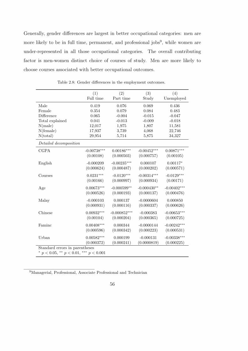
Generally, gender differences are largest in better occupational categories: men are
more likely to be in full time, permanent, and professional jobs9, while women are
under-represented in all those occupational categories. The overall contributing
factor is men-women distinct choice of courses of study. Men are more likely to
choose courses associated with better occupational outcomes.
Table 2.8: Gender differences in the employment outcomes.
(1) (2) (3) (4)Full time Part time Study Unemployed
Male 0.419 0.076 0.069 0.436Female 0.354 0.079 0.084 0.483Difference 0.065 -0.004 -0.015 -0.047Total explained 0.041 -0.013 -0.009 -0.018N(male) 12,017 1,975 1,807 11,581N(female) 17,937 3,739 4,068 22,746N(total) 29,954 5,714 5,875 34,327
Detailed decomposition
CGPA -0.00738∗∗∗ 0.00186∗∗∗ -0.00452∗∗∗ 0.00871∗∗∗
(0.00108) (0.000503) (0.000757) (0.00105)
English -0.000209 -0.00235∗∗∗ 0.000107 0.00117∗
(0.000624) (0.000487) (0.000202) (0.000571)
Courses 0.0231∗∗∗ -0.0120∗∗∗ -0.00314∗∗∗ -0.0129∗∗∗
(0.00166) (0.000997) (0.000934) (0.00171)
Age 0.00673∗∗∗ -0.000599∗∗ -0.000430∗∗ -0.00402∗∗∗
(0.000526) (0.000193) (0.000137) (0.000476)
Malay -0.000103 0.000137 -0.0000604 0.000850(0.000931) (0.000116) (0.000337) (0.000626)
Chinese 0.00932∗∗∗ -0.000852∗∗∗ -0.000383 -0.00653∗∗∗
(0.00104) (0.000204) (0.000365) (0.000725)
Faminc 0.00408∗∗∗ 0.000344 -0.0000144 -0.00242∗∗∗
(0.000596) (0.000342) (0.000223) (0.000531)
Urban 0.00582∗∗∗ 0.000199 -0.000131 -0.00338∗∗∗
(0.000372) (0.000241) (0.0000819) (0.000225)Standard errors in parentheses∗ p < 0.05, ∗∗ p < 0.01, ∗∗∗ p < 0.001
9Managerial, Professional, Associate Professional and Technician
56

Gender differences in full time employment is positive and large, while it is negative
for all the other destinations, showing that men are more likely than women to
be in full time employment. A large portion (63%) of the differences in full time
employment is due to the explained part - the largest contribution is the courses of
study. In previous models we testified that men are more likely to choose courses
that offer better employment prospects. Gender differences in part time employment
is negligible but courses of study remain an important factor10. Women tend to
have higher proportion in choosing to study and choosing self-employment. 60%
of the gender differences in choosing to continue study can be explained by the
observed variables (particularly CGPA and courses) while only 38% of women’s over-
representation in unemployment can be explained by the observed variable (courses
of study). Our finding confirms that women’s inferior employment outcome is partly
due to their choice of courses of study. We may also refute the idea that women’s
lower employment rate is caused by fiercer competition simply because there are
more women in high education. Instead, if women choose Medical, Engineering,
and Computer Science they are more likely to improve their employment prospects.
We proceed with the analysis of gender differences in different job levels among
the employed graduates in Table 2.9. Gender differences is found to be largest
within permanent job level. Again, the largest portion of the difference is due to
the observed characteristics. 74% of the differences can be attributed to graduates’
characteristics and educational attributes. Courses of study contributes more than
half of the explained part. The differences in contract job and self-employment is
negligible. Within temporary jobs, women’s proportion is higher than men where
10The difference between men and women’s participation in part time employment is negative,showing women’s over-representation in that particular occupation by 4% point. There may bethe case where the total explained is larger than the gap itself, for example in column 2. The sumof all contributing variables is a mix of positive and negative coefficients. For example, the sum ofall the coefficients for part time employment is is -0.013 with the courses of study as the largestcontributing factor (-0.012/-0.013).
57
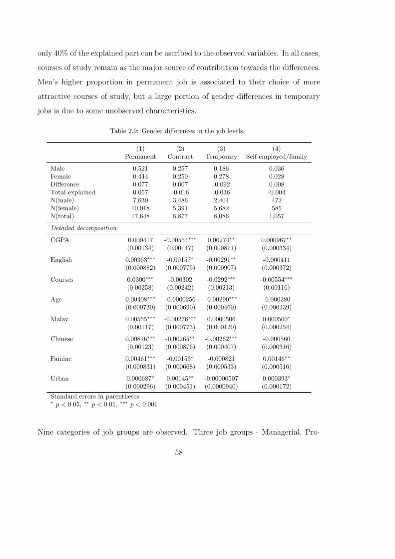
only 40% of the explained part can be ascribed to the observed variables. In all cases,
courses of study remain as the major source of contribution towards the differences.
Men’s higher proportion in permanent job is associated to their choice of more
attractive courses of study, but a large portion of gender differences in temporary
jobs is due to some unobserved characteristics.
Table 2.9: Gender differences in the job levels.
(1) (2) (3) (4)Permanent Contract Temporary Self-employed/family
Male 0.521 0.257 0.186 0.036Female 0.444 0.250 0.278 0.028Difference 0.077 0.007 -0.092 0.008Total explained 0.057 -0.016 -0.036 -0.004N(male) 7,630 3,486 2,404 472N(female) 10,018 5,391 5,682 585N(total) 17,648 8,877 8,086 1,057
Detailed decomposition
CGPA 0.000417 -0.00554∗∗∗ 0.00274∗∗ 0.000967∗∗
(0.00134) (0.00147) (0.000871) (0.000334)
English 0.00363∗∗∗ -0.00157∗ -0.00291∗∗ -0.000411(0.000882) (0.000775) (0.000907) (0.000372)
Courses 0.0300∗∗∗ -0.00302 -0.0292∗∗∗ -0.00554∗∗∗
(0.00258) (0.00242) (0.00213) (0.00116)
Age 0.00408∗∗∗ -0.0000256 -0.00290∗∗∗ -0.000380(0.000730) (0.000690) (0.000460) (0.000239)
Malay 0.00555∗∗∗ -0.00276∗∗∗ 0.0000506 0.000500∗
(0.00117) (0.000773) (0.000120) (0.000254)
Chinese 0.00816∗∗∗ -0.00265∗∗ -0.00262∗∗∗ -0.000560(0.00123) (0.000876) (0.000407) (0.000316)
Faminc 0.00461∗∗∗ -0.00153∗ -0.000821 0.00146∗∗
(0.000831) (0.000668) (0.000533) (0.000516)
Urban 0.000687∗ 0.00145∗∗ -0.00000507 0.000393∗
(0.000296) (0.000451) (0.0000940) (0.000172)
Standard errors in parentheses∗ p < 0.05, ∗∗ p < 0.01, ∗∗∗ p < 0.001
Nine categories of job groups are observed. Three job groups - Managerial, Pro-
58

fessional, Associate Professional and Technician - are considered as ‘higher’ quality
compared to the rest. The differences in the male-female proportion is computed
and detailed decomposition is calculated in Table 2.10. Women are consistently
under-represented in all three superior job groups. Instead, women are found to be
segregated into Administration Support jobs. The proportion of women in Sales are
also higher than men. Half of the gender differences in Professional and Technical
jobs are due to the observed variables such as course of study and CGPA. There
is a significant magnitude of the contribution of courses of study towards gender
differences in professional job group, which help to justify men’s higher proportion
in professional jobs. Fascinatingly, the coefficient for the explained part of gen-
der differences in Managerial job is negative. The peculiarity can be described by
women’s tendency to take Business subject courses which is supposed to strengthen
their share in Managerial job positions. Instead, we find that women are still under-
represented in this particular job group. Our result is consistent with the finding
in Ng and Chakrabarty (2005) and Abdullah et. al. (2008) who found that women
is less preferred in Managerial job positions compared to men. Women are more
likely to be accepted to work as Administration Support workers rather than be-
ing positioned at the centre of organisation (Ng and Chakrabarty, 2005). Women’s
segregation into Administration & Support and Sales jobs are largely due to their
courses of study. The gender difference in Professional Agriculture, Commerce, and
Machinery are negligible. Yet, women are found to be over-represented in basic jobs.
59

Table 2.10: Gender differences in the job groups.
(1) (2) (3) (4) (5)Manager Professional Technician Admin support Sales
Male 0.072 0.576 0.083 0.077 0.109Female 0.064 0.469 0.043 0.220 0.147Difference 0.007 0.108 0.040 -0.143 -0.038Total explained -0.012 0.057 0.024 -0.032 -0.023N(male) 969 8,224 1,301 962 1,492N(female) 1,369 10,593 1,039 4,421 3,092N(total) 2,338 18,817 2,340 5,383 4,584
Detailed decomposition
CGPA 0.00129∗ -0.0181∗∗∗ 0.00235∗∗∗ 0.00149∗∗ 0.00221∗∗∗
(0.000588) (0.00120) (0.000396) (0.000504) (0.000369)
English -0.00214∗ 0.00735∗∗∗ -0.00195 -0.00306∗∗ -0.00206∗
(0.000854) (0.000984) (0.00103) (0.000949) (0.000890)
Courses -0.0146∗∗∗ 0.0644∗∗∗ 0.0157∗∗∗ -0.0306∗∗∗ -0.0277∗∗∗
(0.00152) (0.00243) (0.00150) (0.00179) (0.00178)
Age 0.00104∗ 0.00161∗ -0.000279 0.000233 -0.000487(0.000524) (0.000650) (0.000270) (0.000476) (0.000298)
Malay 0.000685 0.00157 0.000698 0.000569∗ -0.000804(0.000492) (0.00115) (0.00214) (0.000288) (0.00171)
Chinese -0.000542 -0.00319∗ 0.00584∗∗ -0.000824∗∗ 0.00435∗
(0.000429) (0.00129) (0.00226) (0.000283) (0.00191)
Faminc 0.00240∗∗∗ 0.00272∗∗∗ 0.000113 -0.000168 0.00117∗
(0.000722) (0.000724) (0.000387) (0.000447) (0.000569)
Urban -0.0000593 0.000884∗∗∗ 0.00110∗∗ 0.000354 0.000334∗
(0.000134) (0.000220) (0.000348) (0.000355) (0.000142)
(6) (7) (8) (9)Prof. Agri. Commerce Machinery Basic
Male 0.009 0.022 0.005 0.048Female 0.003 0.010 0.004 0.041Difference 0.006 0.012 0.001 0.007Total explained -0.002 0.001 0.000 -0.010N(male) 100 295 65 584N(female) 64 205 73 820N(total) 164 500 138 1,404
Detailed decomposition
CGPA -0.0000739 0.000626∗ 0.000117 0.000836∗∗∗
(0.000271) (0.000265) (0.000123) (0.000243)
English -0.000616 -0.000980∗ 0.0000145 -0.00142∗∗
(0.000380) (0.000417) (0.0000889) (0.000519)
60

Courses -0.00305∗∗∗ 0.000413 -0.000813 -0.00895∗∗∗
(0.000715) (0.000878) (0.000479) (0.00125)
Age -0.000181 -0.000158 0.0000668 -0.000840∗∗
(0.000249) (0.000194) (0.000143) (0.000263)
Malay 0.000132 -0.000468 -0.0000342 0.000218(0.000195) (0.000579) (0.000162) (0.000184)
Chinese -0.000101 0.000233 -0.00000873 -0.000420(0.000112) (0.000630) (0.000228) (0.000245)
Faminc 0.000726∗∗ 0.000392 0.000326 0.000339(0.000279) (0.000223) (0.000182) (0.000317)
Urban 0.000908∗∗∗ 0.000477∗∗ 0.000222 0.000715∗∗∗
(0.000269) (0.000174) (0.000136) (0.000211)
Standard errors in parentheses. ∗ p < 0.05, ∗∗ p < 0.01, ∗∗∗ p < 0.001
61

2.5.3 Gender differences within course of study.
Up to this point, courses of study appear to be the strongest factor that explain
gender differences in graduates first destination choices and employment pattern.
Women’s preference for less attractive courses of study such as Pharmacy, Educa-
tion, and Pure Science11 has detrimental effect on their employment opportunity. If
women posses the same qualification as men, would she be more likely to improve
her employment prospect and reduce their gender differences? Another reason for
women inferior employment rate in our sample is because there are twice the number
of women graduates compared to men (see Ismail (2011)). But if women have the
same qualification, undergone the same training, while controlling for other factors
(i.e. academic achievement, English, SES) the prevailing gender differences may
either signify statistical discrimination towards women or may indicate taste. The
policy implication of women enrolment into higher education by merit alone may
just do more harm, encouraging unnecessary investment in tertiary education for
some women if there is no action taken to rectify gender differences in employment
opportunity.
To test whether gender differences exist among graduate possessing similar qual-
ification, we compute gender differences in full time and part time employment
within each course of study. Table 2.11 shows the result for full time employment
and Table 2.12 for part time employment. We found evidence of gender differ-
ences between courses of study and its variation is more profound in the full time
employment as shown in Table 2.11. In full time employment, men are found to
be over-represented in courses such as: Law, Transport, Computer Sciences and
Engineering while women are over-represented in Arts & Social Science, Manage-
11The employment rates for Pharmacy, Education, and Pure Science are 32%, 34%, and 39%,respectively and the ratio women to men is almost 4:1.
62

ment, and Administration. The over-representation of men in Computer Science
can be ascribed by the observed variables which make up 40% of the differences,
leaving a large portion to some unexplained part. The worse can be seen in Law,
Transport and Engineering where the observed variables only explains between 17%
(Engineering) to 22% (Transport) of the variation. Women’s over-representation in
Administration is largely ascribable to their characteristics. But only 11% of the
women’s over-representation in Art & Social Science and 27% in Management can
be explained by the observed variables, the larger portion remain unexplained.
The magnitude of gender differences in part time employment is small compared to
full time employment, indicating that the pattern for part time employment is more
uniformly distributed among men and women. We found moderate differences in
several courses, particularly men are found to be over-represented in Nurse, Jour-
nalism, and Education with very low percentage of the explained part - indicating
that within these courses the propensity for men who took part time jobs are due to
some unmeasured attributes. Women who took Transport and Pure Science courses
are over-represented in part time employment, largely due to their characteristics
which explain 89% and 51% of the variation, respectively.
The finding shows that even though women have the same qualification as men,
they are still under-represented in full time employment despite their investment in
highly technical courses such as Engineering and Computer Sciences. The differences
in full time employment are attributable to some unmeasured components - which
may also be a potential discrimination towards women with these qualifications.
The situation is worse for women with Engineering qualification. Indeed, women
have higher participation in full time employment when they took courses such as
Art & Social Science and Management - which are characterised by low employment
prospect and low pay.
63

Tab
le2.1
1:
Gen
der
diff
eren
ces
wit
hin
each
cou
rse
of
stu
dy
-fu
llti
me
emp
loym
ent
Law
Art
s/S
ocS
cT
ran
sport
Ad
min
istr
ati
on
Man
agem
ent
Eco
nom
yA
ccou
nta
ncy
Mark
etin
g
Mal
e0.
355
0.1
95
0.6
36
0.4
85
0.3
68
0.3
79
0.5
71
0.4
20
Fem
ale
0.24
30.2
19
0.5
26
0.4
98
0.3
88
0.3
51
0.5
50
0.3
46
Diff
eren
ce0.
113
-0.0
24
0.1
10
-0.0
13
-0.0
21
0.0
28
0.0
21
0.0
73
Tot
alex
pla
ined
0.02
3-0
.003
-0.0
25
0.0
11
-0.0
05
0.0
22
0.0
05
0.0
43
%ex
pla
ined
20%
11%
22%
83%
27%
78%
26%
59%
N(m
ale)
346
879
77
1002
1594
414
837
379
N(f
emal
e)79
92485
133
2411
5126
1040
2687
858
N(t
otal
)11
453364
210
3413
6720
1454
3524
1237
Fin
ance
Jou
rnali
smIs
lam
icF
ood/h
osp
itali
tyA
rts
Pu
resc
ien
ceA
pp
lied
scie
nce
Ph
arm
acy
Mal
e0.
449
0.4
16
0.2
88
0.4
24
0.2
44
0.2
88
0.0
91
0.3
26
Fem
ale
0.39
00.4
21
0.2
78
0.3
79
0.2
26
0.2
39
0.0
97
0.2
81
Diff
eren
ce0.
059
-0.0
06
0.0
10
0.0
45
0.0
18
0.0
49
-0.0
06
0.0
45
Tot
alex
pla
ined
0.03
60.0
06
0.0
21
-0.0
24
0.0
24
0.0
46
-0.0
26
0.0
21
%ex
pla
ined
61%
104%
205%
55%
136%
93%
421%
46%
N(m
ale)
853
385
243
295
594
267
154
1233
N(f
emal
e)22
891037
659
850
1118
904
505
3301
N(t
otal
)31
421422
902
1145
1712
1171
659
4534
Med
ical
Den
tist
ryN
urs
eE
nvir
on
men
tS
port
sE
ngin
eeri
ng
Com
pS
ciE
du
cati
on
Mal
e0.
639
0.1
88
0.3
70
0.3
60
0.2
58
0.4
79
0.5
48
0.1
82
Fem
ale
0.58
30.1
45
0.3
73
0.3
03
0.2
21
0.3
87
0.4
51
0.1
59
Diff
eren
ce0.
056
0.0
43
-0.0
04
0.0
57
0.0
36
0.0
92
0.0
98
0.0
23
Tot
alex
pla
ined
0.02
5-0
.022
-0.0
33
0.0
00
0.0
53
0.0
16
0.0
39
0.0
25
%ex
pla
ined
46%
49%
878%
0%
146%
17%
40%
109%
N(m
ale)
626
69
165
491
159
7319
1658
1241
N(f
emal
e)12
19207
790
999
131
5802
2405
3877
N(t
otal
)18
45276
955
1490
290
13121
4063
5118
Sta
nd
ard
erro
rsin
par
enth
eses
.∗p<
0.0
5,∗∗p<
0.01,∗∗
∗p<
0.001
64
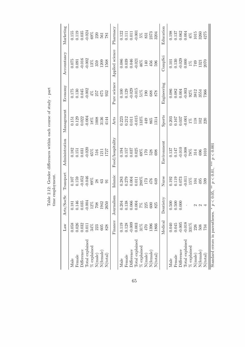
Tab
le2.1
2:
Gen
der
diff
eren
ces
wit
hin
each
cou
rse
of
stu
dy
-p
art
tim
eem
plo
ym
ent.
Law
Art
s/S
ocS
cT
ran
sport
Ad
min
istr
ati
on
Man
agem
ent
Eco
nom
yA
ccou
nta
ncy
Mark
etin
g
Mal
e0.
058
0.1
81
0.1
07
0.1
82
0.1
51
0.1
75
0.0
75
0.1
55
Fem
ale
0.02
60.1
46
0.1
59
0.1
51
0.1
29
0.1
30
0.0
91
0.1
19
Diff
eren
ce0.
032
0.0
35
-0.0
52
0.0
31
0.0
22
0.0
45
-0.0
16
0.0
35
Tot
alex
pla
ined
0.01
1-0
.004
-0.0
46
-0.0
20
-0.0
04
-0.0
02
-0.0
02
-0.0
24
%ex
pla
ined
34%
12%
89%
65%
18%
4%
13%
69%
N(m
ale)
223
708
28
516
1008
257
359
220
N(f
emal
e)60
51942
63
1211
3136
675
1209
561
N(t
otal
)82
82650
91
1727
4144
932
1568
781
Fin
ance
Jou
rnali
smIs
lam
icF
ood
/h
osp
itality
Art
sP
ure
scie
nce
Ap
pli
edsc
ien
ceP
harm
acy
Mal
e0.
119
0.2
04
0.2
83
0.1
94
0.2
23
0.1
00
0.0
86
0.1
22
Fem
ale
0.12
80.1
38
0.2
79
0.1
57
0.2
12
0.1
29
0.0
39
0.1
11
Diff
eren
ce-0
.009
0.0
66
0.0
04
0.0
37
0.0
11
-0.0
29
0.0
46
0.0
11
Tot
alex
pla
ined
0.00
30.0
04
0.0
11
0.0
25
-0.0
15
-0.0
15
-0.0
21
-0.0
01
%ex
pla
ined
31%
7%
288%
69%
133%
51%
46%
5%
N(m
ale)
470
225
173
170
449
190
140
831
N(f
emal
e)13
96600
476
528
865
688
456
2373
N(t
otal
)18
66825
649
698
1314
878
596
3204
Med
ical
Den
tist
ryN
urs
eE
nvir
on
men
tS
port
sE
ngin
eeri
ng
Com
pS
ciE
du
cati
on
Mal
e0.
040
0.5
00
0.1
92
0.1
37
0.2
03
0.0
86
0.1
01
0.1
98
Fem
ale
0.04
50.5
00
0.1
19
0.1
47
0.1
67
0.0
82
0.1
30
0.1
37
Diff
eren
ce-0
.005
0.0
00
0.0
73
-0.0
10
0.0
37
0.0
04
-0.0
29
0.0
62
Tot
alex
pla
ined
-0.0
18.
-0.0
11
-0.0
08
-0.0
01
-0.0
03
0.0
00
0.0
04
%ex
pla
ined
331%
15%
78%
1%
92%
1%
6%
N(m
ale)
226
2104
314
118
3812
749
1015
N(f
emal
e)50
82
495
696
102
3554
1321
3260
N(t
otal
)73
44
599
1010
220
7366
2070
4275
Sta
nd
ard
erro
rsin
par
enth
eses
.∗p<
0.05,∗∗p<
0.01,∗∗
∗p<
0.001
65

2.5.4 Gender segregation by industry.
This part examines industrial variations in gender segregation among our sample
graduates. Twenty one industries were included in the the analysis. The differences
in the employment outcomes between male and female graduates within each indus-
try are reported in Table 2.13 for full time employment and Table 2.14 for part time
employment.
Consistent with the finding in (Osman and Shahiri, 2014), the evidence for dis-
crimination for women graduates within Manufacturing sector is prevalent. Women
are under-represented in Construction, Manufacturing, Scientific / Technical, IT /
Communication, and Electric / Gas / Steam industries - all of which are heavily
industrialised sector associated with high skilled workers and high paying jobs. In-
terestingly, a large portion of the differences in the full time employment within
these sectors are ascribable to some unmeasured factors which may signify discrimi-
nation or taste (considering these jobs are very demanding). The situation is worse
for Construction and Manufacturing industries. Instead, we found women are segre-
gated towards Education, Finance / Insurance, Administration Support, and other
services. Again, large portion of male-female difference in full time employment
within these sectors are unexplained (probably unmeasured taste). These sectors
are also found to be associated with low employment rate, more heterogenous job
prospects and low paying jobs.
The magnitude of gender differences is even bigger in part time employment shown
in Table 2.14 where women are inclined to have part time employment more than
men in industries such as Agriculture / Forestry / Fishing, Food / Hospitality, and
Transport / Storage. In the other hand, men have higher proportion in part time
employment in industries such as IT / Communication, Social work, and Wholesale
- which are largely explained by graduates’ characteristics.
66
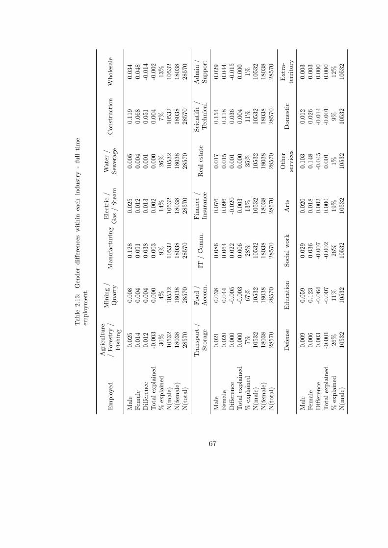
Tab
le2.1
3:
Gen
der
diff
eren
ces
wit
hin
each
ind
ust
ry-
full
tim
eem
plo
ym
ent.
Em
plo
yed
Agr
icu
ltu
re/
For
estr
y/
Fis
hin
g
Min
ing
/Q
uarr
yM
anu
fact
uri
ng
Ele
ctri
c/
Gas
/S
team
Wate
r/
Sew
erage
Con
stru
ctio
nW
hole
sale
Mal
e0.
025
0.0
08
0.1
28
0.0
25
0.0
05
0.1
19
0.0
34
Fem
ale
0.01
40.0
04
0.0
91
0.0
12
0.0
04
0.0
68
0.0
48
Diff
eren
ce0.
012
0.0
04
0.0
38
0.0
13
0.0
01
0.0
51
-0.0
14
Tot
alex
pla
ined
-0.0
030.0
00
0.0
03
0.0
02
0.0
00
0.0
04
-0.0
02
%ex
pla
ined
30%
4%
9%
14%
26%
7%
13%
N(m
ale)
1053
210532
10532
10532
10532
10532
10532
N(f
emal
e)18
038
18038
18038
18038
18038
18038
18038
N(t
otal
)28
570
28570
28570
28570
28570
28570
28570
Tra
nsp
ort
/S
tora
ge
Food
/A
ccom
.IT
/C
om
m.
Fin
an
ce/
Insu
ran
ceR
eal
esta
teS
cien
tifi
c/
Tec
hn
ical
Ad
min
/S
up
port
Mal
e0.
021
0.0
38
0.0
86
0.0
76
0.0
17
0.1
54
0.0
29
Fem
ale
0.02
00.0
44
0.0
64
0.0
96
0.0
15
0.1
18
0.0
44
Diff
eren
ce0.
000
-0.0
05
0.0
22
-0.0
20
0.0
01
0.0
36
-0.0
15
Tot
alex
pla
ined
0.00
0-0
.003
0.0
06
0.0
03
0.0
00
0.0
04
0.0
00
%ex
pla
ined
7%67%
28%
13%
35%
11%
1%
N(m
ale)
1053
210532
10532
10532
10532
10532
10532
N(f
emal
e)18
038
18038
18038
18038
18038
18038
18038
N(t
otal
)28
570
28570
28570
28570
28570
28570
28570
Def
ense
Ed
uca
tion
Soci
al
work
Art
sO
ther
serv
ices
Dom
esti
cE
xtr
a-
terr
itory
Mal
e0.
009
0.0
59
0.0
29
0.0
20
0.1
03
0.0
12
0.0
03
Fem
ale
0.00
60.1
23
0.0
36
0.0
18
0.1
48
0.0
26
0.0
03
Diff
eren
ce0.
003
-0.0
64
-0.0
07
0.0
02
-0.0
45
-0.0
14
0.0
00
Tot
alex
pla
ined
-0.0
01-0
.007
-0.0
02
0.0
00
0.0
01
-0.0
010.0
00
%ex
pla
ined
26%
11%
26%
19%
1%
9%
12%
N(m
ale)
1053
210532
10532
10532
10532
10532
10532
67

N(f
emal
e)18
038
18038
18038
18038
18038
18038
18038
N(t
otal
)28
570
28570
28570
28570
28570
28570
28570
68

Tab
le2.1
4:
Gen
der
diff
eren
ces
wit
hin
each
ind
ust
ry-
part
tim
eem
plo
ym
ent.
FT
/P
T
Agr
icu
ltu
re/
For
estr
y/
Fis
hin
g
Manu
fact
uri
ngEle
ctri
c/
Gas
/S
team
Con
stru
ctio
nWh
ole
sale
Tra
nsp
ort
/S
tora
ge
Food
/A
ccom
.IT
/C
om
m.
Fin
an
ce/
Insu
ran
ce
Mal
e0.
679
0.9
28
0.9
19
0.9
23
0.7
04
0.8
72
0.5
53
0.9
11
0.9
32
Fem
ale
0.84
80.9
17
0.9
22
0.9
55
0.6
86
0.9
56
0.6
84
0.8
75
0.9
32
Diff
eren
ce-0
.169
0.0
11
-0.0
03
-0.0
32
0.0
18
-0.0
85
-0.1
31
0.0
35
0.0
00
Tot
alex
pla
ined
-0.0
430.0
06
0.0
22
0.0
08
0.0
50
0.0
01
-0.0
17
0.0
23
0.0
08
%ex
pla
ined
25%
60%
710%
25%
280%
1%
13%
65%
6874%
N(m
ale)
265
1353
259
1250
358
218
405
906
797
N(f
emal
e)24
41634
218
1223
866
365
788
1153
1724
N(t
otal
)50
92987
477
2473
1224
583
1193
2059
2521
Rea
les
tate
Sci
enti
fic
/T
ech
nic
al
Ad
min
/S
up
port
Def
ense
Ed
uca
tion
Soci
al
work
Art
sO
ther
serv
ices
Dom
esti
c
Mal
e0.
880
0.9
48
0.8
20
0.8
28
0.5
60
0.8
87
0.6
48
0.7
68
0.6
61
Fem
ale
0.92
10.9
30
0.8
18
0.8
30
0.5
47
0.8
55
0.7
29
0.7
87
0.6
74
Diff
eren
ce-0
.041
0.0
18
0.0
02
-0.0
02
0.0
13
0.0
32
-0.0
82
-0.0
19
-0.0
13
Tot
alex
pla
ined
-0.0
090.0
03
0.0
31
0.0
48
0.0
25
0.0
41
-0.0
17
0.0
13
0.0
38
%ex
pla
ined
22%
15%
1556%
2332%
190%
129%
21%
70%
297%
N(m
ale)
175
1623
306
99
621
309
213
1081
124
N(f
emal
e)27
72127
787
112
2210
656
329
2667
460
69

2.5.5 Ethnic differences by industry.
One continuous dilemma in Malaysia is due to the imbalance proportion of ethnic
share in the country where ethnic groups are still identified with economic activities
(Osman and Shahiri, 2014), (Osman-Rani, 1982). Unlike other socially heterogenous
countries where the ethnic minority usually have lower employment rate, in Malaysia
it is the ethnic majority, the aborigine that lack participation in the labour market
and are associated with lower earning. This section investigates ethnic share in
different types of occupations especially among high technological industries which
require high skilled workers to carry out the job tasks. Theoretically we suppose that
education, particularly higher education, should be able to remedy the imbalance
for ethnic differences in the employment outcome and enhance social mobility within
high technological industries. Our results shows that Malays remain at the economic
disadvantage by working in the low-skilled industries compared to Chinese who are
over-represented in high-skilled industries.
The results for ethnic differences in the employment outcome within each industry is
given by Table 2.15-Table 2.17. The top part shows ethnic differences in employment
status within each industry between the Malays and all other ethnic groups, while
the lower part shows ethnic differences between the Chinese and all other ethnic
groups. The result is almost parallel to each other - Malay’s over-representation in
one industry is related to Chinese’s under-representation in that industry, and vice
versa. The Chinese are over-represented in high skilled industries such as Scientific
/ Technical, Manufacturing, Finance / Insurance, and IT / Communication sectors.
These sectors are also associated with higher average income. Ethnic differences in
IT / Communication and Finance / Insurance are largely explained by graduates’
attributes but only 21% of the differences in Manufacturing and 41% in Scientific
/ Technical can be explained by the observed variables. One important variable
70

that may explain the variation is parental education and occupations, otherwise the
difference may signify potential discrimination. On the other hand, Malays are over-
represented in industries such as Education, Administration Support, Wholesale,
and other services. Malay’s segregation into Education and other services industries
are largely explained by their characteristics. However, their over-representation
in Administration Support is largely due to some unmeasured observations. In
general, we found evidence of ethnic segregation to some extent within industries -
the Chinese show tendency towards highly skilled and high paying industries, while
the Malays show tendency towards low skilled and low paying industries.
71

Tab
le2.1
5:
Eth
nic
diff
eren
ces
wit
hin
each
ind
ust
ry.
(1)
(2)
(3)
(4)
(5)
(6)
(7)
Agr
icu
ltu
re/
For
estr
y/
Fis
hin
g
Min
ing
/Q
uarr
yM
anu
fact
uri
ng
Ele
ctri
c/
Gas
/S
team
Wate
r/
Sew
erage
Con
stru
ctio
nW
hole
sale
Oth
er0.
015
0.0
06
0.1
32
0.0
15
0.0
03
0.0
84
0.0
32
Mal
ay0.
019
0.0
06
0.0
91
0.0
18
0.0
05
0.0
88
0.0
48
Diff
eren
ce-0
.005
0.0
00
0.0
42
-0.0
02
-0.0
01
-0.0
04
-0.0
17
Tot
alex
pla
ined
-0.0
070.0
01
0.0
09
-0.0
04
-0.0
01
-0.0
04
-0.0
05
%ex
pla
ined
1.45
02.6
05
0.2
10
1.6
42
0.9
93
0.8
72
0.2
77
N(o
ther
)16
572
1,4
98
227
42
1,1
14
396
N(m
alay
)38
8133
2,2
01
481
115
2,0
41
1,0
17
N(t
otal
)55
3205
3,6
99
708
157
3,1
55
1,4
13
Agr
icu
ltu
re/
For
estr
y/
Fis
hin
g
Min
ing
/Q
uarr
yM
anu
fact
uri
ng
Ele
ctri
c/
Gas
/S
team
Wate
r/
Sew
erage
Con
stru
ctio
nW
hole
sale
Oth
er0.
020
0.0
06
0.0
89
0.0
18
0.0
05
0.0
87
0.0
48
Ch
ines
e0.
010
0.0
06
0.1
51
0.0
14
0.0
03
0.0
85
0.0
26
Diff
eren
ce0.
011
0.0
00
-0.0
62
0.0
04
0.0
02
0.0
03
0.0
23
Tot
alex
pla
ined
0.00
3-0
.003
-0.0
06
0.0
00
0.0
00
0.0
08
0.0
09
%ex
pla
ined
0.29
07.9
63
0.1
04
0.1
16
0.0
48
3.0
70
0.4
21
N(o
ther
)46
9155
2,4
52
558
130
2,2
99
1,1
57
N(c
hin
ese)
8450
1,2
47
150
27
856
256
N(t
otal
)55
3205
3,6
99
708
157
3,1
55
1,4
13
72

Tab
le2.1
6:
Eth
nic
diff
eren
ces
wit
hin
each
ind
ust
ry.
(8)
(9)
(10)
(11)
(12)
(13)
(14)
Tra
nsp
ort/
Sto
rageF
ood
/A
ccom
.IT
/C
om
m.
Fin
an
ce/
Insu
ran
ceR
eal
esta
teS
cien
tifi
c/
Tec
hn
ical
Ad
min
/S
up
port
Oth
er0.
019
0.0
32
0.0
77
0.1
04
0.0
12
0.1
70
0.0
26
Mal
ay0.
021
0.0
47
0.0
70
0.0
80
0.0
18
0.1
12
0.0
44
Diff
eren
ce-0
.003
-0.0
15
0.0
07
0.0
24
-0.0
06
0.0
58
-0.0
18
Tot
alex
pla
ined
-0.0
01-0
.010
0.0
10
0.0
22
0.0
03
0.0
24
-0.0
01
%ex
pla
ined
0.43
80.6
29
1.5
23
0.9
28
0.4
78
0.4
09
0.0
45
N(o
ther
)25
5432
963
1,2
50
146
2,0
50
355
N(m
alay
)51
3970
1,6
67
1,8
44
368
2,7
34
999
N(t
otal
)76
81,4
02
2,6
30
3,0
94
514
4,7
84
1,3
54
Tra
nsp
ort/
Sto
rageF
ood
/A
ccom
.IT
/C
om
m.
Fin
an
ce/
Insu
ran
ceR
eal
esta
teS
cien
tifi
c/
Tec
hn
ical
Ad
min
/S
up
port
Oth
er0.
021
0.0
48
0.0
70
0.0
80
0.0
16
0.1
11
0.0
43
Ch
ines
e0.
017
0.0
23
0.0
79
0.1
13
0.0
14
0.1
91
0.0
23
Diff
eren
ce0.
004
0.0
25
-0.0
09
-0.0
33
0.0
03
-0.0
80
0.0
21
Tot
alex
pla
ined
0.00
00.0
09
-0.0
12
-0.0
23
0.0
00
-0.0
40
0.0
09
%ex
pla
ined
0.11
10.3
48
1.3
39
0.7
02
-0.1
23
0.5
06
0.4
29
N(o
ther
)59
71,1
35
1,9
04
2,1
13
392
3,1
05
1,1
20
N(c
hin
ese)
171
267
726
981
122
1,6
79
234
N(t
otal
)76
81,4
02
2,6
30
3,0
94
514
4,7
84
1,3
54
73

Tab
le2.1
7:
Eth
nic
diff
eren
ces
wit
hin
each
ind
ust
ry.
(15)
(16)
(17)
(18)
(19)
(20)
(21)
Def
ense
Ed
uca
tion
Soci
al
work
Art
sO
ther
serv
ices
Dom
esti
cE
xtr
a-
terr
itory
Oth
er0.
003
0.0
79
0.0
35
0.0
20
0.1
19
0.0
14
0.0
04
Mal
ay0.
010
0.1
09
0.0
33
0.0
18
0.1
37
0.0
24
0.0
02
Diff
eren
ce-0
.007
-0.0
30
0.0
02
0.0
02
-0.0
19
-0.0
09
0.0
01
Tot
alex
pla
ined
-0.0
04-0
.023
0.0
10
-0.0
04
-0.0
18
-0.0
05
-0.0
01
%ex
pla
ined
0.63
00.7
72
4.9
09
2.0
44
0.9
46
0.5
03
-0.8
66
N(o
ther
)35
989
529
278
1,5
64
165
47
N(m
alay
)20
42,5
24
840
416
3,0
92
493
56
N(t
otal
)23
93,5
13
1,3
69
694
4,6
56
658
103
Def
ense
Ed
uca
tion
Soci
al
work
Art
sO
ther
serv
ices
Dom
esti
cE
xtr
a-
terr
itory
Oth
er0.
009
0.1
11
0.0
33
0.0
19
0.1
38
0.0
23
0.0
03
Ch
ines
e0.
001
0.0
63
0.0
35
0.0
20
0.1
11
0.0
13
0.0
03
Diff
eren
ce0.
008
0.0
48
-0.0
01
-0.0
01
0.0
27
0.0
10
-0.0
01
Tot
alex
pla
ined
0.00
30.0
26
-0.0
05
0.0
02
0.0
07
0.0
05
0.0
00
%ex
pla
ined
0.36
10.5
41
3.3
79
1.4
58
0.2
50
0.4
73
0.8
00
N(o
ther
)22
82,9
26
992
484
3,5
47
544
70
N(c
hin
ese)
11587
377
210
1,1
09
114
33
N(t
otal
)23
93,5
13
1,3
69
694
4,6
56
658
103
74
2.6 Conclusion.
The expansion of higher learning institution which leads to the proliferation in ter-
tiary education enrolment is motivated by the need for high skilled workers to fulfil
the demand for high technological jobs, but also bring with it problems with rising
unemployment among its graduates. Universities and the policy makers have collab-
orated to understand the determinants of graduate’s employability. Many studies
found various factors that influence individual’s success in obtaining his first job
after education. This paper contributes to the literature in terms of the use of a
wider spectrum of analysis that cover large categories of occupational types which
are not limited to a binary employed-unemployed category. The innovative aspect
of this paper is when we disentangle the gender differences within each course of
study to investigate if women with the same qualification as men would have similar
employment opportunity.
In this chapter, we confirm many studies that found that graduate academic achieve-
ment, English language ability, and other social and economic status such as family
income, locality, and ethnic also play a major role in determining graduate’s first
destination choice as well as their employment pattern. Higher academic achieve-
ment and better English proficiency, which is also related to individual’s ability are
also associated with better employment outcomes. Older age, Chinese, and higher
family income - lead to high full time employment and decreases unemployment.
But higher family income also lead to self-employment among graduates who work
in family businesses. Generally, we found that courses of study play a major role in
graduate’s employment outcomes.
We found the evidence of gender differences in full time employment but within
part time employment the distribution of men and women graduates are almost
75

uniform, though women tend to have a higher proportion in choosing to study and
self-employment. Women’s under-representation in superior occupations (full time,
permanent, professional, and managerial) is due to their chosen course of study
(Pharmacy, Pure Science, Education)12. Women’s segregation into Administration
& Support and Sales jobs are largely due to their courses of study. Women are also
found to be over-represented in basic jobs.
The finding shows that even though women have the same qualification as men in
highly technical courses such as Engineering and Computer Sciences, they are still
under-represented in full time employment. The differences in full time employment
are attributable to some unmeasured components - which may also be a potential
discrimination towards women with these qualifications.
We also found evidence of discrimination for women graduates within Manufacturing
sector which is consistent with the finding by Osman and Shahiri (2014). Women
are under-represented in heavily industrialised sector associated with high skilled
workers and high paying jobs. Indeed, women are found to be segregated into
services sectors. The gender inequality in employment opportunity may signify
either discrimination or taste - that women may have chosen less demanding jobs in
order to balance between family and work.
The policy implication of women enrolment into higher education by merit alone
may just do more harm if it is only encouraging unnecessary investment in tertiary
education for some women when there is no action taken to rectify gender differences
in employment opportunity. In the case of women who possess similar qualification
as men but end up in the lower occupational category, we haven’t been able to
measure whether the pattern is due to taste/preference or discrimination. In the
12The employment rates for Pharmacy, Education, and Pure Science are 32%, 34%, and 39%,respectively and the ratio women to men is almost 4:1.
76

case of taste, qualified women may take attractive courses such as Engineering but
intentionally choose low demanding jobs. But if it is due to discrimination, especially
in the case of the private sector (i.e. Manufacturing), necessary actions need to
be taken to devise a policy that will reduce the imbalance participation rate by
encouraging female labour force participation in those industries. In the case of
Malaysia, women have the same right as men (same working hours, no employment
ban) but women’s lower employment rate in high skilled industries is perhaps due
to restrictions such as maternity leave, small children, avoiding dangerous jobs, and
cultural expectation. If that is the case, we need to reinforce policies to support
women’s employment such as the implementation of maternity and paternity leave
(so that childcare is distributed equally between parents), encourage flexible working
hours, and the provision of childcare facilities.
Finally, we also found evidence of ethnic segregation within industries - the Chinese
show tendency towards highly skilled jobs in the high paying industries, while the
Malays show a tendency towards low skilled and low paying industries. The con-
tinuity of imbalance proportion of ethnic share in the country where ethnic groups
are identified with economic activities still remains among graduates of tertiary
education. Theoretically, we suppose that education should be able to remedy the
imbalance for ethnic differences in the employment outcome, especially in high tech-
nological industries. We showed that Malay’s inferior employment outcome due to
their choice of courses which may stem from their under-achievement at schools -
high scorers among school leavers were accepted in selective universities and selec-
tive courses. Family influence also plays a significant role where families who see the
importance of education will emphasis school achievement which leads to gaining
entry to superior education which will eventually lead to successful employment.
Generally, we found Malay’s and women’s inferior employment outcomes because
77

of their choice of courses, where sorting into such courses originated from their
lower academic performance at schools. Malays generally come from rural origin
where education quality is lower, the physical environment is poor, low parental
education and occupation which affect they way individual behave for their choice
of education and work. University quota in student intake does not seem to help
because Malay tends to take less attractive courses associated with less demanding
jobs, which is also conditional on their poorer performance in school. Majority
Malays took Malay studies, Islamic studies, and Arts & Social Sciences which have
limited practicability in the economy. One way to reduce unemployment among
these groups might be to reduce the intake of courses that are not demanded by the
labour market and instead increase the participation into STEM courses. If a student
is not qualified to enter university and take up such courses, then vocational training
must be promoted. Courses that are less demanded should not be entirely banished
due to their contribution towards social benefits and knowledge creation, but the
admission into such courses should be limited in order to reduce the incidence of
over-education where graduate receive the wrong signal and they invest in education
that does not help them in their career.
78

2.7 Appendix.
79

Tab
le2.1
8:
Em
plo
ym
ent
ou
tcom
esam
on
ggra
du
ate
s.
Male
gra
du
ate
sF
emale
gra
du
ate
s(1
)(2
)(3
)(4
)(1
)(2
)(3
)(4
)F
ull
tim
eP
art
tim
eS
tud
yU
nem
plo
yed
Fu
llti
me
Part
tim
eS
tud
yU
nem
plo
yed
Art
s/S
ocS
c-0
.107∗∗
∗0.0
827∗
∗∗-0
.243∗∗
∗0.2
67∗∗
∗0.0
135
0.0
862∗∗
∗-0
.341∗∗
∗0.2
42∗∗
∗
Tra
nsp
ort
0.26
6∗∗
∗-0
.00486
-0.2
48∗∗
∗-0
.0136
0.2
62∗∗
∗0.0
525∗
-0.3
47∗∗
∗0.0
318
Ad
min
istr
atio
n0.
118∗∗
∗0.0
519∗
∗∗-0
.253∗∗
∗0.0
836∗
∗0.2
39∗∗
∗0.0
548∗
∗∗-0
.350∗∗
∗0.0
563∗
∗
Man
agem
ent
0.04
91
0.0
385∗
∗-0
.242∗∗
∗0.1
55∗∗
∗0.1
71∗∗
∗0.0
511∗
∗∗-0
.349∗∗
∗0.1
26∗∗
∗
Eco
nom
y0.
0461
0.0
607∗
∗-0
.229∗∗
∗0.1
22∗∗
∗0.1
25∗∗
∗0.0
595∗
∗∗-0
.334∗∗
∗0.1
50∗∗
∗
Acc
ounta
ncy
0.19
2∗∗
∗-0
.00834
-0.2
50∗∗
∗0.0
661∗
0.2
83∗∗
∗0.0
218∗
∗-0
.348∗∗
∗0.0
431∗
Mar
keti
ng
0.04
91
0.0
531∗
∗-0
.243∗∗
∗0.1
41∗∗
∗0.0
911∗
∗∗0.0
564∗
∗∗-0
.337∗∗
∗0.1
89∗∗
∗
Fin
ance
0.10
6∗∗
∗0.0
199
-0.2
48∗
∗∗0.1
23∗∗
∗0.1
65∗∗
∗0.0
523∗
∗∗-0
.340∗∗
∗0.1
23∗∗
∗
Jou
rnal
ism
0.04
60
0.0
761∗
∗∗-0
.244∗∗
∗0.1
22∗∗
∗0.1
43∗∗
∗0.0
625∗
∗∗-0
.356∗∗
∗0.1
50∗∗
∗
Isla
mic
-0.0
00116
0.1
15∗∗
∗-0
.253∗∗
∗0.1
38∗∗
∗0.0
842∗
∗∗0.1
63∗∗
∗-0
.353∗∗
∗0.1
07∗∗
∗
Food
/hos
pit
alit
y0.
0921∗
0.0
585∗
∗-0
.250∗∗
∗0.0
994∗
∗0.1
49∗∗
∗0.0
736∗
∗∗-0
.364∗∗
∗0.1
42∗∗
∗
Art
s-0
.0709∗
0.0
934∗
∗∗-0
.241∗∗
∗0.2
18∗∗
∗0.0
195
0.1
26∗∗
∗-0
.353∗∗
∗0.2
07∗∗
∗
Pu
resc
ien
ce-0
.0583
0.0
325
-0.1
99∗∗
∗0.2
25∗∗
∗0.0
369
0.0
711∗∗
∗-0
.314∗∗
∗0.2
06∗∗
∗
Ap
pli
edsc
ien
ce-0
.0103
0.0
405∗
∗-0
.226∗∗
∗0.1
96∗∗
∗0.0
625∗
∗∗0.0
568∗
∗∗-0
.322∗∗
∗0.2
02∗∗
∗
Ph
arm
acy
-0.2
64∗∗
∗0.0
550
0.1
46∗∗
0.0
630
-0.1
46∗
∗∗0.0
192
0.0
429
0.0
843∗∗
Med
ical
0.21
5∗∗
∗-0
.0116
-0.1
27∗∗
∗-0
.0764∗
0.3
06∗∗
∗0.0
118
-0.2
38∗
∗∗-0
.0789∗∗
∗
Den
tist
ry-0
.211∗∗
∗0.0
171
0.0
761
0.1
18
-0.1
03∗
∗∗-0
.0129
0.0
507
0.0
652
Nu
rse
0.00
866
0.0
903∗
∗-0
.273∗∗
∗0.1
74∗∗
∗0.1
23∗∗
∗0.0
612∗
∗∗-0
.329∗∗
∗0.1
45∗∗
∗
Envir
onm
ent
0.03
64
0.0
385∗
-0.2
43∗∗
∗0.1
68∗∗
∗0.0
924∗
∗∗0.0
788∗
∗∗-0
.336∗∗
∗0.1
64∗∗
∗
Sp
orts
-0.0
590
0.0
824∗
∗-0
.257∗∗
∗0.2
34∗∗
∗0.0
212
0.0
972∗∗
∗-0
.365∗∗
∗0.2
46∗∗
∗
En
gin
eeri
ng
0.12
1∗∗
∗0.0
00290
-0.2
29∗
∗∗0.1
07∗∗
∗0.1
53∗∗
∗0.0
269∗
∗∗-0
.324∗∗
∗0.1
44∗∗
∗
Com
pS
ci0.
173∗∗
∗0.0
0575
-0.2
33∗
∗∗0.0
545
0.2
04∗∗
∗0.0
496∗
∗∗-0
.340∗∗
∗0.0
856∗
∗∗
Ed
uca
tion
-0.1
43∗∗
∗0.1
06∗
∗∗-0
.184∗∗
∗0.2
21∗∗
∗-0
.0629∗∗
∗0.0
994∗
∗∗-0
.266∗∗
∗0.2
29∗∗
∗
Ob
serv
atio
ns
21280
21280
21280
21280
41632
41632
41632
41632
Sta
nd
ard
erro
rsin
par
enth
eses
∗p<
0.05
,∗∗p<
0.01
,∗∗
∗p<
0.0
01
80

Tab
le2.1
9:
Job
leve
lsam
on
ggra
du
ate
s.
Male
gra
du
ate
sF
emale
gra
du
ates
(1)
(2)
(3)
(4)
(1)
(2)
(3)
(4)
Per
man
ent
Contr
act
Tem
pora
ryS
elf-
emplo
yed
Per
man
ent
Contr
act
Tem
por
ary
Sel
f-em
plo
yed
Art
s/S
ocS
c0.
0232
0.0
0180
-0.0
803
0.0
553∗∗
-0.0
0868
0.1
22∗∗
∗-0
.156∗∗
∗0.0
427∗
∗∗
Tra
nsp
ort
0.27
2∗∗∗
0.0
882
-0.3
66∗
∗∗0.0
0525
0.2
08∗∗
∗0.1
55∗∗
-0.3
59∗∗
∗-0
.00486
Ad
min
istr
atio
n0.
290∗
∗∗-0
.0124
-0.3
03∗∗
∗0.0
253
0.2
11∗∗
∗0.1
18∗∗
∗-0
.355∗∗
∗0.0
257∗
∗∗
Man
agem
ent
0.18
5∗∗∗
0.0
478
-0.2
59∗
∗∗0.0
262∗
0.1
66∗∗
∗0.1
34∗∗
∗-0
.316∗∗
∗0.0
158∗
∗
Eco
nom
y0.
0785
0.0
717
-0.2
02∗
∗∗0.0
522∗
0.1
11∗∗
0.1
30∗∗
∗-0
.274∗∗
∗0.0
337∗
∗
Acc
ounta
ncy
0.36
1∗∗∗
-0.0
243
-0.3
39∗∗
∗0.0
0184
0.3
26∗∗
∗0.0
551∗
-0.3
93∗∗
∗0.0
123∗
Mar
keti
ng
0.18
7∗∗∗
0.0
629
-0.3
18∗
∗∗0.0
681∗∗
0.1
80∗∗
∗0.1
38∗∗
∗-0
.321∗∗
∗0.0
0351
Fin
ance
0.18
0∗∗∗
0.0
946∗
-0.2
88∗∗
∗0.0
138
0.1
59∗∗
∗0.1
74∗∗
∗-0
.363∗∗
∗0.0
296∗
∗∗
Jou
rnal
ism
0.15
4∗∗
0.0
839
-0.2
64∗
∗∗0.0
259
0.1
22∗∗
∗0.1
92∗∗
∗-0
.328∗∗
∗0.0
150
Isla
mic
-0.0
0529
0.0
557
-0.1
11
0.0
604∗
-0.1
34∗∗
∗0.1
28∗∗
∗-0
.049
80.0
557∗
∗∗
Food
/hos
pit
alit
y0.
265∗
∗∗-0
.0799
-0.2
35∗∗
∗0.0
498∗
0.2
14∗∗
∗0.0
507
-0.2
94∗∗
∗0.0
295∗
∗
Art
s0.
122∗
-0.0
396
-0.1
37∗
∗0.0
543∗∗
-0.0
0761
0.0
896∗∗
-0.1
36∗∗
∗0.0
544∗
∗∗
Pu
resc
ien
ce0.
183∗
∗-0
.0105
-0.1
81∗
∗0.0
0816
0.0
648
0.0
911∗
∗-0
.189∗∗
∗0.0
335∗
∗
Ap
pli
edsc
ien
ce0.
173∗
∗∗0.0
534
-0.2
66∗
∗∗0.0
390∗∗
0.1
37∗∗
∗0.0
848∗
∗-0
.251∗∗
∗0.0
294∗
∗∗
Ph
arm
acy
-0.1
01-0
.120
0.1
91
0.0
288
0.0
593
-0.0
690
-0.0
784
0.0
881∗
Med
ical
0.35
0∗∗∗
-0.1
45∗∗
∗-0
.191∗∗
∗-0
.0139
0.3
08∗∗
∗-0
.0466
-0.2
68∗
∗∗0.0
0660
Den
tist
ry0.
357∗
-0.2
45∗∗
∗-0
.359∗∗
∗0.2
47
0.3
82∗∗
∗-0
.118∗
∗-0
.386∗∗
∗0.1
21
Nu
rse
0.16
9∗∗
0.0
535
-0.2
21∗
∗∗-0
.00154
0.1
28∗∗
∗0.0
919∗
∗-0
.274∗∗
∗0.0
549∗
∗∗
Envir
onm
ent
0.22
4∗∗∗
0.0
190
-0.2
86∗
∗∗0.0
426∗
0.1
13∗∗
0.0
835∗
∗-0
.232∗∗
∗0.0
358∗
∗∗
Sp
orts
0.15
5∗0.0
0272
-0.1
69∗
0.0
112
0.0
890
0.0
795
-0.1
83∗
0.0
144
En
gin
eeri
ng
0.31
4∗∗∗
0.0
139
-0.3
41∗
∗∗0.0
130
0.2
63∗∗
∗0.1
10∗∗
∗-0
.385∗∗
∗0.0
117∗
Com
pS
ci0.
265∗
∗∗0.0
628
-0.3
46∗
∗∗0.0
176
0.1
86∗∗
∗0.1
92∗∗
∗-0
.390∗∗
∗0.0
123∗
Ed
uca
tion
-0.0
0271
-0.0
427
0.0
0267
0.0
427∗
∗-0
.121∗∗
∗0.0
501
0.0
327
0.0
381∗
∗∗
Ob
serv
atio
ns
1053
210532
10532
10532
18038
18038
18038
18038
Sta
nd
ard
erro
rsin
par
enth
eses
∗p<
0.0
5,∗∗p<
0.01
,∗∗
∗p<
0.001
81

82
Chapter 3
Wage differentials across sectors,
gender, and ethnic groups.
3.1 Introduction.
There are large empirical literatures in studying the public-private sector wage dif-
ferences with mixed findings supporting the evidence of public sector wage premium
(Bender, 2003),(Bender and Elliot, 1999),(Disney and Gosling, 2008),(Azam et. al,
2013),(Tansel, 2005),(Terrel, 1993),(Seshan, 2013); or the evidence of wage premium
in the private sector (Heitmueller, 2004); the evidence that the public sector pay
less than the private sector especially among university graduates (Adamchik, 1999);
and the greater emphasis in investigating the variance of the differential distribu-
tion instead of the overall differences (Melly, 2005)(Bender, 2003). To date there
has been very little studies on the public-private sector wage differential in the
Southeast Asia. Specifically, there was only two studies conducted in Malaysia -
Mazumdar (1981) using 1975 data, and more recent study by Seshan (2013) us-
83

ing 2007 Malaysian Household Income Survey. One aspect of this chapter seeks to
contribute to the literature by addressing the public-private sector wage differential
among the high skilled workers in Malaysia and investigate the evidence of public
sector wage premium among university graduates in the country. My finding shows
distinct discovery than Seshan (2013) in a sense that there is no evidence of public
sector wage premium among university graduates. The different outcomes from both
studies can be attributed to the different sample being used. My study is rather
consistent with (Adamchik, 1999) who found no evidence of public pay premium
among university graduates.
Despite the increasing number of women in tertiary education, gender gap still per-
sists even in developed countries. Nonetheless, it is also important to note that
there has been reduction in gender pay gap over the years. Women enrolment in
Malaysian tertiary education is doubled compared to men, but women’s participa-
tion in employment and their remuneration still lag behind. Several reasons can
be used to explain the disparity: first, women have tendency to choose less attrac-
tive courses of study that are usually associated with blurred employment prospect
and low pay compared to men’s preferences towards highly technical and attractive
courses of study. Second, women face greater competition simply because there
are greater number of women in tertiary education in the country. In order to in-
vestigate whether gender pay gap exists among Malaysian university graduates, we
investigate male-female wage gap in different settings. The finding shows that the
gender pay gap exists in the private sector labour market, where male graduates
earn significantly higher than females and the difference is accounted for by some
unexplained factors, suggesting potential evidence of discrimination towards women
in the private sector. We also found evidence of discrimination towards women
in Manufacturing and Defence industries, while men face discrimination in Food /
Accommodation industry.
84

Ethnic polarisation is still a heated argument in the country. Due to historical
division by ethnic group prior to Independence, one common assumption that con-
tinues to hold is that the Malays and the indigenous are more preferable to gain
employment and better remuneration in the public sector; while Chinese are more
preferable in the private sector labour market. One aspect of this paper investigates
the wage differential by ethnic groups in the public and private sector labour market
to test if the assumption holds. My finding informs that, consistent with the public
policy that do not practice discrimination, we found no evidence of ethnic wage dif-
ferential in the public sector. However, we found significant wage premium between
all other groups compared to the Malays in the private sector. The difference is
found to be largely due to some unexplained factors.
The measurement of graduate earning in this study was taken a few months after
finishing study. Some graduates have experienced a very successful transition into
full time employment, but due to the narrow time frame between finishing study
and the time the survey was conducted, a fraction of graduates found themselves
land on a transitory, rather than perpetual job to begin their career. The last part
of this chapter investigates wage premium among graduates who obtained full time
employment at the time the survey was conducted compared to those who work part
time. The finding shows the evidence of wage premium among full time workers with
male premium larger than female. The difference is however largely accounted for
by full time worker’s superior characteristics.
The chapter is related to a literature that points toward the earning differences in
the public-private sector labour market among youth. This paper also speaks to
the literature on graduate’s gender and ethnic pay gap. As mentioned before, there
is little empirical studies done in Southeast Asian due to the lack of data avail-
ability. This paper contributes to the literature by correcting the selectivity bias
85

in the earning equation where the earning is only observed among those who are
employed. Estimating a pooled earning equation by including a dummy variable
for each group (i.e. sector, gender, and race) restrict all other coefficients to be the
same for all groups which is unlikely, hence alternative method should be applied.
Indeed, separate wage equation can be estimated for both group and then use the
results to decompose the differences in the average income into two portions. One
portion represents the difference in the average worker characteristics and job at-
tributes, another represents the difference in the returns to workers characteristics
and their job attributes. The former explains the differences in wages between two
workers having different characteristics, where we would expect worker with higher
productive ability and/or job that compensate for equalising difference to earn more.
The latter explains the differences in the earning among two workers possessing sim-
ilar characteristics and job attributes and hence may provide potential evidence of
discrimination. To my knowledge this is the first study of graduates that exten-
sively analyse graduate earning in various ways. Previous literatures in the research
on Malaysian graduates rarely examine the earning and instead largely focused on
graduate’s employability.
The chapter will be organised as follows: Section 3.2 discusses theoretical issues
related to the earning function (Section 3.2.1), previous studies on public-private
labour market (Section 3.2.2), gender pay gap (Section 3.2.3), and a short his-
torical description related to economic share of different ethnicity in Malaysia (Sec-
tion 3.2.4). Section 3.4 introduces the econometric framework, and finally Section 3.5
discusses the results. The chapter is closed with a conclusion.
86
3.2 Background and previous researches.
3.2.1 Earning function, equalising difference, and wage de-
termination.
The human capital earning function pioneered by Mincer in 1974 has work so well in
the empirical regularities to study the effect of investment in schooling and on-the-
job training on productivity-related earnings. Workers who invest more to acquire
skills through schooling have to face opportunity costs in terms of forgone earning
and direct costs of school tuition and hence it is highly relevant for these workers
to be compensated with a higher lifetime earnings for their increased productivity
through the investment in schooling and training. A possible deficiency in the human
capital theory can be explained by the positive relationship between ability and years
of schooling where individual who spent more years in schooling also possess higher
ability, and ability translates into higher productivity and hence higher earning
which then places an upward bias in rate of return to schooling. In the case of
university graduates, years of schooling alone is inadequate to explain the return
to education because of the existence of different effect of different course of study
(Walker and Zhu, 2001). Heterogenous returns across different course of study can
be explained by certain course of study that is associated with higher ability. These
courses offer distinct and high skilled workers for labour market. Individuals with
more intensive course of study possess higher ability which translate into higher
productivity. Medical, Dentistry, and Engineering graduates for example already
posses higher ability before starting university and their courses are more intense
compared to others.
In the study of earnings differences between individuals the theory of equalising
differences may explain the equalisation of monetary and non-monetary gain (or
87
lose) among different job attributes. In the labour market transaction workers and
employers each simultaneously choose job attributes and worker’s attributes, respec-
tively, to achieve an acceptable match where preferred choice of workers and em-
ployers are met. In a situation where productively homogenous workers are choosing
between two jobs - one is pleasant, and one is unpleasant - in making the decision
the workers are taking the rational and optimal choice for a preferred job based on
how much income must be compensated so that the worker may be indifference to
take up the less preferred job. This level of income is called the reservation wage or
the shadow price to compensate for the unpleasantness of the job attributes associ-
ated with the less desirable job. The unpleasant job attributes may be explained by
hazardous working conditions, unusual working hours, and jobs that require specific
set of skills that have to be acquired through years of training and high level of in-
tensity such as medical and law professions. The undesirable attributes of jobs can
also be explained by the geographical location where certain location may provide
better living conditions such as amenities and lower living costs compared to other
locations (Rosen, 1999).
The persistence of wage difference due to discrimination can be observed in sys-
tematic and consistent disparity of income between groups of workers that may be
attributed by gender, race, and other social attributes. In the economic discrimina-
tion concept, the term minority describes a group who experience lesser economic
rewards, and the term majority describes the favourable group. Discrimination is
defined as two workers possessing similar productivity-related attributes but getting
paid differently, and the difference is persistent based on the minority’s demographic
profile. Employers and other worker’s taste for discrimination which translate into
unequal employment and earning opportunity among minority workers is what is
termed as prejudice. Workers within the same firm may practice prejudice if they
abstain from working with the minority workers, which may cause job segregation
88

where the minorities are more concentrated in different type of jobs. Consumer may
also be another source of discrimination when they abstain from being served with
minority workers (Cain, 1999).
3.2.2 Public-private sector labour market.
In the study of wage differential in the public-private sector labour market, Gregory
and Borland (1999) provides an extensive discussion on the unique nature of public
sector labour market in terms of its objective, ownership, production, and operation.
Governments are generally the largest employer of a country. Its operation involves
large expenditure which is financed primarily through taxes and borrowing, hence
calling for the public concern over the efficiency (Bender, 2003).
There are a number of possibility that public-private differences and how it may
affect the earning determination between those sectors might be of interest. Wage
determination between the two sectors are different, due to the difference in the
functionality and size of both establishments. Unlike their private sector counter-
parts, governments are lack of profit motives. They do not only produce goods
and services, Borjas (1980) also believed that bureaucrats are also involved in elec-
toral process and producing votes, hence may justify higher pay (Gunderson, 1980).
Public sector may produce goods and services not available elsewhere, allowing for
monopolistic market for its production.
The political environment provide means for achieving specific government objec-
tives, while the private sector’s objectives is restricted by the market environment.
While the private sector objective is to minimise production costs, the public sector
objectives can be classified into three types of concentration. Public sector that
concern with the maximisation of social welfare will seek to resolve labour market
89

imperfection by introducing equal policy and affirmative action to reduce discrimina-
tion. Bureaucrats will seek to maximise budget allocation. Politicians may seek for
vote maximisation. Hence, hiring and earning decision made by politicians would be
different than if the decision is made to maximise efficiency (Gregory and Borland,
1999).
As a model employer the government may also offer low-skilled workers with higher
rates, but might be adverse to paying too high if the public does not like to see
government workers earning too much. Women and minority often benefit most
by being employed in the public sector (Bender, 2003). Bender (2003) also suggest
that overpaying government workers results in waste in public budget, but offering
too low results in incapability to recruit and retain skilled and productive workers.
It is difficult to identify attributes of workers who seek employment in the public
sector from those who obtain the job. Bellante and Link (1981) found evidence of
public sector workers being more risk averse. However Gregory and Borland (1999)
provides another perspective that perhaps the employers in the public sector are
more keen to hire workers who are risk averse and more loyal. Public sector labour
market also allow scope for welfare-type activities. The consequence is it make it
difficult to identify the unobserved motivation of workers who seek employment in
the public sector for reasons related to the welfare goals.
There are evidence of public sector employees being paid more than equally pro-
ductive private sector employees at the lower earning distribution, while the reverse
is observed at the higher earning distribution (Katz and Krueger, 1992). Studies
found that there is a double imbalance in the public-private sector pay comparison.
Workers at the lower end of the occupational hierarchy receive higher pay in public
sector, but earn less at the upper end of the earnings compared to private sector
workers (Bender, 2003)(Katz and Krueger, 1992)(Elliott, Robert and Duffus, 1996).
90

There are a number of reasons why the public sector may provide better pay scheme
to its workers. Certain types of public sector occupations do not exist in the private
sector hence the government uses the highest wage in order to attract workers who
would otherwise choose private sectors. For certain occupations, it is impossible to
appropriately classify and survey the jobs in other sector hence lead to an upward
bias in public sector wage. While deciding wage structure, public sector often do not
consider the non-monetary benefits that is being offered to their workers, resulting in
the government ‘paying compensating differentials when they are not needed’ (Fogel
and Lewin, 1974). However, given the persistence of the unexplained portion of wage
differentials between public-private sector wages which is ‘too unlikely’, Moore and
Raisian (1981) suggested that the premiums are due to skill differentials between
workers of both sectors.
Many previous literatures attempted to decompose wage differential into a portion
accounted for by differences in productivity-related factors that individuals bring
to the labour market and a residual that presumably represents labour market dis-
crimination (Daymont and Andrisani, 1984). Borland, Gregory and Sheehan (2001)
provides an extensive cross-country analysis on the differentials. The overall find-
ing from various literatures found that the results depend on country differences
and model specifications. Some studies provided mixed results on the overall wage
differences, another focused on the differences in the distribution of the wage and
found that the variance is an important element that needs to be included in study-
ing public-private wage differential because public sector wage is more compress
(Melly, 2005). This is important especially in the case of a double imbalance in
pay distribution where government workers are paid more at the lower end of the
wage distribution, and less at the higher end of the distribution (Katz and Krueger,
1992).
91

Private sector is a key driver of economic growth in most Southeast Asian countries.
However at the moment, there has been very little research done on public-private
wage differentials in Southeast Asia. Recent study in Malaysia using Malaysia
Household Income Survey from 1995 to 2007, Seshan (2013) reported that in 1995
the average public-private wage ratio is 1.12, and by 2007 it has grown to 1.29.
After controlling for individual characteristics, public sector employees were found
to earn some unexplained wage premium, particularly higher starting wage. Instead
of rewarding its workers based on productivity, public sector is found to reward its
workers for the length of service. Public sector employees are found to be older, with
more work experience, and better educated. Women in both sectors posses better
education than men, and women’s wage premium working in a public sector is higher
than men. There is greater gender wage gap in the private sector favouring men, in
contrast, the gender wage gap is lower in the public sector. The large unexplained
gender pay gap in the private sector suggesting wage discrimination against women.
3.2.3 Gender pay gap
Gender pay gap and job discrimination against women have received a lot of atten-
tion and continue to gain widespread attention across the world. The exclusion of
women in male occupations leads to an “overcrowding” of women in certain jobs,
at the same time create job segregation for women in certain occupation. Following
this, the devaluation theory suggests that women’s lower status contribute to the
lower wage setting in “female” jobs. The devaluation theory implies employer’s view
on occupation with high proportion of women as less valuable, resulting in low pay
determination (England, Allison and Wu, 2007). Because of employer’s preference
for men in most jobs, women were forced to choose less attractive occupations hence
explaining their lower earning. Based on a study using Current Population Survey
92
in 2007, England, Allison and Wu (2007) show that given workers’ preference, em-
ployers is more likely to take men for high paying jobs since they can easily able to
get men. On the other hand for low paying occupations employers is more likely
to take women since men are already more likely to be accepted for high paying
jobs. Women face obstacle to high paying jobs and are blocked from receiving equal
pay especially at the higher end of income distribution, creating a condition which
is called as the “glass ceiling” (Albrecht et. al., 2001) especially at managerial job
position (Jurajda and Paligorova, 2006).
From sociological perspective women are viewed to play important role as a carer in
the family, not a breadwinner. Becker (1985) and Polachek (1976) suggested that
women’s rational decision for family care and child bearing lead them into investing
less in human capital accumulation. Women also choose to seek less demanding
job since house works undertaken by women is quite an intensive energy consuming
labour. Interruptions due to child birth which cause human capital decay among
women also causes women to have less labour market experience compared to men.
However, following massive expansion of higher education it is found that women are
now more educated than men. McDaniel (2012) reported that young women perform
better in academic achievement than young men. Indeed, UNESCO (2012) reported
that young women’s aspiration is now higher than young men in terms of career
progression. With the deceleration of marital institution women are now taking
shorter break from employment and hence should have close their wage gap with
men especially in full-time employment (Makepeace and Pal, 2004). Nonetheless
the persistence of gender wage gap causes some women to be more vulnerable to
over-education (Figueiredo et. al, 2015).
A meta-analysis on gender pay gap by Weichselbaumer (2005) utilising more than
260 published papers from 63 countries between 1960s to 1990s found that the raw
93

wage differentials have fallen from 65% to 30%, largely characterised by women’s pro-
gressive attributes such as better education and work attachment. From the sources
of the published papers being investigated, the unexplained component shows no
decline over time. However, the meta-regression analysis uses specification for a
standardised method including data selection suggested an actual discrimination is
actually lower. They also found that data restrictions seriously affect statistical re-
sult of gender pay gap. Studies using data of a particular group of respondent who
are never married, new entrant to the job market, or workers in narrow occupations
provide better comparability and result in lower wage differential. However, omitted
variables such as complete record of human capital characteristics (i.e. on-the-job
training and job tenure) can result in serious bias. Studies that do not include work
experience can seriously overestimate the unexplained wage gap.
One major mis-specification in the existing empirical literatures is the inability of
human capital function to measure ability, which is also correlated with schooling
(Griliches, 1977). Using schooling as a measure of attributes assumes all individu-
als have similar distribution of the courses taken at the university while in fact men
were more likely to study in engineering and business, while women were more likely
to study education, liberal arts, and social sciences (Brown and Corcoran, 1997).
Courses of study play an important role in the structure of wage in specialised hu-
man capital. Investing in specialised human capital require more relinquishment
than ordinary human capital and hence we would expect workers with acquisition
of specialised human capital should receive higher return (Becker, 1971). Another
important measure that may explain wage differentials is inter-industry character-
istics. Firm characteristics exert influence on discrimination against women (Tam,
1997)(Becker, 1975). Firm specific information may provide better measures of
workers ability hence may better explain wage differentials (Altonji and Blank,
1999)(Zanchi, 1998). We overcome these mis-specification by controlling for dif-
94

ferent courses of study. We also compute wage differential within each industry to
obtain finer results in the wage differentials.
In Malaysia, Nagaraj (2014) studied 120 establishments in manufacturing industry
within the region of Klang Valley (most industrialised and developed region in the
country) found evidence of raw difference in the male-female earnings but the result
is doubtful due to omitted variable and sample selection bias using the restricted
data. An earlier study in Malaysia by Chapman and Harding (1985) suggested that
there has been very low studies involving developing countries, and surprisingly the
finding is somewhat similar to that of the developed countries. Using data from the
Economic Planning Unit, the study found that there was a systematic difference
in education and experience among men and women and hence women earned less
because they had lower skills (but keep in mind that the study was conducted
more than 30 years ago). But it was also evident that employers practiced wage
discrimination within particular job where women were rewarded at a lower rate.
Women were also found to be employed in relatively low-paying jobs. Chapman and
Harding (1985) offered two reasons on the difficulty to concur with the existence of
discrimination. First, it is difficult to determine to what extent does the employer
practice discrimination towards women workers. Women high turnover can be the
cause towards their lower earning, however if it becomes the determinant towards
the overall women’s wage then women at large might be statistically discriminated.
Secondly, if certain occupation offer lower pay, it is also difficult to look at the
difference between employer’s allocation and worker’s own choice. It is possible that
women socialisation processes such as tradition and education before entering the
labour market influence their decision to choose certain types of occupations that
are characterised by low wage.
In his paper Chapman and Harding (1985) concluded that women received higher
95

rate of returns for their primary and secondary schooling, while men received higher
rate of return for tertiary education. Each year increase in experience gave higher
return for men. Men also received higher return for on-the-job training and each
hour worked. Married men earned 6% increase in wage, but for married women
the change in wage was insignificant. However migration to the capital city Kuala
Lumpur benefited women more than men. Based on these finding, Chapman and
Harding (1985) reckoned that by providing women with more education will not
necessarily reduce their pay gap. Chapman and Harding (1985) conceded that since
the study focused on young workers (average age is 27) hence it may not be possible
to generalise the result to the whole population.
3.2.4 Ethnic wage gap.
Malaysia is a special case of a segmented plural society with persistent ethnic in-
equality in terms of societal rewards such as earning (dominated by Chinese) and
political power (dominated by Malays). Chronically, as a consequence of British
colonisation in the then Malaya between 1786 to 1957, a large number of Chinese
and Indians were brought to work in tin mining and rubber estates for the British
ruler. Residential location and occupations were stratified by ethnic group. The
Chinese established small towns for tin mining, wage labourers, artisans, traders,
and merchants. The Indians were located around rubber estates and oil palm plan-
tations. Malays remained in agriculture as farmers and fishermen, further hamper
their possibility to gain education in the cities, where education may cause upris-
ing. Rather, Malays attended orthodox religious schools in their villages. English
schools were introduced in the towns where Chinese, Indians and a minority Malay
aristocrats had had better access to English education. English-language was also
a prominent language in trade and industry and hence those who attended English
96

schools have an upward occupational mobility (Ong, 2012).
Malays once regained their power in 1957 (Independence) had to compete with Chi-
nese and Indians who had a head start in economy. Residential segregation during
the British colonisation persisted after the Independence. Strong intergenerational
occupation immobility shows that father’s occupation played an influential role in
their offsprings’ success. Intergenerational occupational inheritance is strong in all
ethnic group. Chinese were more likely to follow their fathers in non-agricultural
jobs and succeeding their fathers’ occupations in the cities. Malays were more likely
to stay in the agriculture following their birth of origin and their fathers’ occu-
pation. The trend for Indians were intermingled between the two, some were still
working in the rubber estates and plantations, and some moved the city. Location of
birth and fathers’ occupation were the main determinant of children’s occupations.
Hirschman (1983) found strong intergenerational immobility leading to job segrega-
tion and ethnic stratification. Occupational attainment depended largely on social
origin. The structural opportunity block in ethnic-based recruitment in sales and
retail restrained the Malays from entering such occupations. Hirschman (1983) also
found that Malays were also under-represented in commerce, manufacturing, and
prestigious white collar occupations (i.e. professional, administration, and clerical)
where Chinese were more privileged to take up such occupations due to living in an
urban state and family ties (i.e. ownership and management of shops and factories).
It is a common knowledge that less advantageous group is thought to be lacking in
motivation and aspiration. If this is the case then policy need to be established to
increase their values and aspirations. However Hirschman (1983) found no evidence
for a certain group’s lacking in motivation or ambition to be the cause for their being
less advantageous in economy rather than their intergenerational mobility limitation
and place of origin. If ethnicity alone become the barrier towards employment in
97

certain type of occupation then no any kind of intervention can remedy the problem
(Hirschman, 1983), as in the case for sales occupations. Hence Hirschman (1983)
suggested that direct policy in terms of setting quotas to assure ethnic proportions
would lessen the discrimination.
Intervention action should be looking at the adjustment criteria in recruiting and
promoting. To make sure that socioeconomic status is not linked to ethnicity, ed-
ucational opportunity and training should be expanded for the less advantageous
group (Hirschman, 1983). Indeed, equalising socioeconomic for all ethnic actually
neutralise the intergenerational process. The availability of jobs in the urban/rural
setting has a major impact on the job opportunity for certain ethnic group due
to geographical segregation. If the job creation in the rural setting is implausible
then it is important to promote migration to the city. In small establishments kin
recruitment is common. When economic unit grow and become more bureaucratic,
the hiring pattern become more universalistic (Hirschman, 1983).
Persistent ethnic inequality coupled with structural poverty will seriously harm the
country. The serious ethnic-economic disparity reached its peak when the tension
caused an ethnic riot in 1969. To remedy the problem of economic disparity, the
government introduced a New Economic Policy (NEP) targeting to eradicate poverty
among all ethnic groups and “to restructure society to abolish the identification of
race with economic function” (see Second Malaysia Plan (1971)). The NEP coined
the term “Bumiputera” to acknowledge Malays and the indigenous of Sabah and
Sarawak as the sons of the soil which grant them special rights in economy and
education. The plan included preferential treatment towards the Bumiputeras in
terms of education, employment, business, and ownership. In education an elite
Majlis Amanah Rakyat (MARA) Junior Science Colleges, Fully Residential Schools,
Science Secondary Schools, and a number of pre-university and tertiary education
98

institutions were opened exclusively for the Bumiputeras (Ong, 2012). Enrolment
into public university also increased dramatically due to ethnic quota into university.
Intervention in employment saw the establishment of Industrial Coordination Act
(1975) which regulates 30% of Bumiputera employment quota in private sector. The
legislation transformed private sector in terms of ownership, workers recruitment,
and licensing under the purview of Ministry of Trade and Industry.
However the result of implementation NEP received various responses. NEP was
found to be able to reduce ethnic gap and reduce Malay poverty to a certain extent
where it is evident over a generation we observed the occurrence of Malay urban
middle class entering professional occupations. On the other hand, NEP received
heavy criticism from the non-Malays who are being recognised as second class citizen
due to the Malay supremacy. Some opined that NEP was Malay’s agenda to mak-
ing sure Malay’s special position in the land for their acknowledgement of Chinese
and Indians as citizen. However, instead of benefiting the low income Bumiputeras,
Selvaratnam (1988) found that the NEP has indeed benefitted the mostly urban
middle class especially in education. Then again Jomo (2004) found that govern-
ment special consideration on Malays have actually benefited among the politicians
and politically-connected businessmen. Only in the public sector that NEP seems
to be able to eradicate Malay’s poverty - employment in the public sector increased
to almost double with the creation of public enterprises in various industries. Even
though public sector offer lower wages but it is compensated for greater job security
and better pension plan. The lower proportion of non-Malays in the public sector is
due to common perception of unequal chances in recruitment and promotion (Ong,
2012). The trend sees Malays dominating the public sector, while Chinese domi-
nating the private sectors (Jomo, 2004). Nevertheless, Nagaraj (2014) found that
after the NEP the intra-ethnic wage gap worsened especially among Malays. It is
also found that education, employment and politic remain entangled with ethnicity.
99

NEP’s preferential treatment towards Malays in public university and public sector
jobs created brain drain where a lot of non-Malays choose to study or work abroad.
A study on ethnic economic gap and the impact of NEP by Shahiri (2012) found
that occupation segregation have reduced for all ethnic group by the end of NEP im-
plementation. However, ethnic wage gap continue to rise especially between Malays
and Chinese in all types of occupations. The study utilises various sources of data
from West Malaysian Family Survey, First Malaysian Family Life survey, Second
Malaysian Family Life Survey, Population Census of Peninsular Malaysia, and Pop-
ulation and Housing Census of Malaysia. Using Oaxaca decomposition technique,
the study concludes that NEP does not succeeded in reducing ethnic wage gap
between all ethnic groups except between Malay and Indians in professional and
agricultural sectors. Chinese remains benefitting highest income in every type of
occupations.
3.2.5 Full time wage premium.
The final part of this chapter discusses the wage premium among the employed
graduates. Graduate’s employment status is observed within the narrow time frame
after they finished their studies. Some graduates found themselves landed on a tem-
porary job before they obtain more suitable job with their qualification. During this
waiting room effect some graduates found themselves experiencing over-education
by taking up part-time or temporary jobs at the beginning of their career (Dekker
et. al., 2002). We computed the difference between graduates who work full time
compared to those who work part time. Obviously, wage premium among full time
workers is significant and large. However we cannot conclude the subsequent effect
of part time job penalty because we do not observe graduate’s career mobility for
several years ahead. The part time workers among graduates may accept the first
100

job offer in order to gain experience and then use this job as a stepping stone before
they take up more suitable job in the future (Rosen, 1972).
3.3 Data.
The data used in this chapter is obtained from the 2013 Graduate Tracer Study
conducted by the Ministry of Higher Education Malaysia. The data is described
earlier in Section 2.3. We remove non-first degree graduates, disabled graduates, and
non-citizen from the data, leaving us with 69,995 graduates with 35,668 reported as
employed at the time the survey data is taken. Table 3.1 shows the observed wage
among our sample graduates - public sector wage is bimodal at RM501-RM1,500 and
RM3,001-RM5,000, while private sector wage distribution is located in the middle
income group (RM1,501-RM2,501).
Table 3.1: Public and private sector wage distribution among sample graduates.
Graduate income Public Percent Private Percent
< RM 500 249 0.05 1,291 0.04RM 501 - RM 1000 1,057 0.22 4,466 0.14RM 1001 - RM 1500 1,072 0.23 4,759 0.15RM 1501 - RM 2000 568 0.12 7,269 0.24RM 2001 - RM 2500 285 0.06 7,160 0.23RM 2501 - RM 3000 299 0.06 4,234 0.14RM 3001 - RM 5000 1,150 0.24 1,514 0.05> RM 5000 78 0.02 217 0.01Total 4758 1.00 30,910 1.00
Table 3.2 shows some descriptive statistics on courses of study. The largest group in
our sample is graduates who took Engineering course which make up a quarter of all
individuals. The top five courses of study are: Engineering, Management, Computer
Sciences, Education, and Applied Science. The average employment rate is 51%.
101
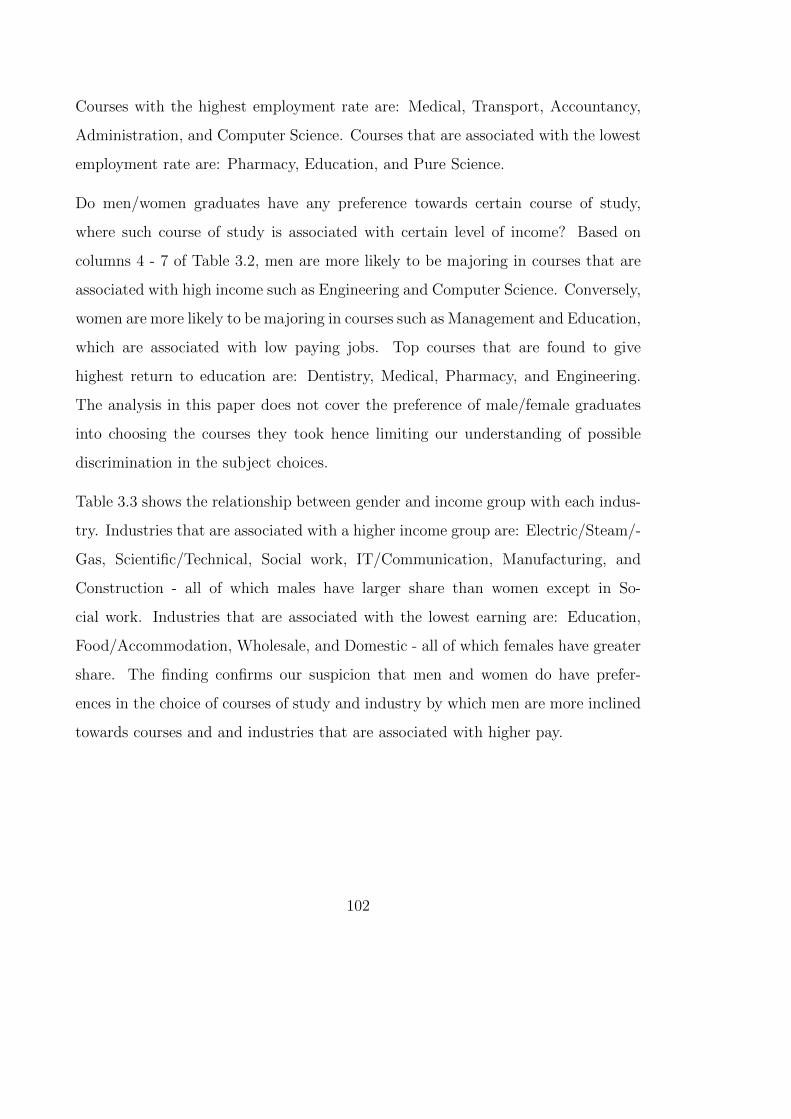
Courses with the highest employment rate are: Medical, Transport, Accountancy,
Administration, and Computer Science. Courses that are associated with the lowest
employment rate are: Pharmacy, Education, and Pure Science.
Do men/women graduates have any preference towards certain course of study,
where such course of study is associated with certain level of income? Based on
columns 4 - 7 of Table 3.2, men are more likely to be majoring in courses that are
associated with high income such as Engineering and Computer Science. Conversely,
women are more likely to be majoring in courses such as Management and Education,
which are associated with low paying jobs. Top courses that are found to give
highest return to education are: Dentistry, Medical, Pharmacy, and Engineering.
The analysis in this paper does not cover the preference of male/female graduates
into choosing the courses they took hence limiting our understanding of possible
discrimination in the subject choices.
Table 3.3 shows the relationship between gender and income group with each indus-
try. Industries that are associated with a higher income group are: Electric/Steam/-
Gas, Scientific/Technical, Social work, IT/Communication, Manufacturing, and
Construction - all of which males have larger share than women except in So-
cial work. Industries that are associated with the lowest earning are: Education,
Food/Accommodation, Wholesale, and Domestic - all of which females have greater
share. The finding confirms our suspicion that men and women do have prefer-
ences in the choice of courses of study and industry by which men are more inclined
towards courses and and industries that are associated with higher pay.
102

Table 3.2: Graduate’s employment, gender, and income level by courses of study.
Courses N%
EmployedMale Female
% <RM2,000
% >RM2,000
Law 969 0.50 1.25 1.46 0.42 0.58Arts/SocSc 3,860 0.40 3.91 6.44 0.32 0.68Transport 240 0.67 0.36 0.33 0.42 0.58Administration 4,243 0.60 5.29 6.51 0.36 0.64Management 6,899 0.50 6.64 11.71 0.37 0.63Economy 1,519 0.49 1.78 2.4 0.33 0.67Accountancy 4,293 0.65 4.32 7.18 0.40 0.60Marketing 1,336 0.50 1.73 2.01 0.31 0.69Finance 3,286 0.51 3.65 5.29 0.32 0.68Journalism 1,727 0.52 1.8 2.85 0.30 0.70Islamic 954 0.51 1.05 1.54 0.48 0.52Food/hospitality 1,355 0.55 1.54 2.17 0.43 0.57Arts 1,818 0.42 2.5 2.65 0.38 0.62Pure science 1,139 0.39 1.05 1.96 0.28 0.72Applied science 4,542 0.42 4.92 7.39 0.29 0.71Pharmacy 457 0.32 0.43 0.78 0.15 0.85Medical 2,059 0.74 2.8 3.02 0.08 0.92Dentistry 189 0.46 0.23 0.29 0.04 0.96Nurse 1,218 0.49 0.84 2.26 0.30 0.70Environment 1,425 0.44 1.89 2.12 0.33 0.67Sports 307 0.40 0.69 0.29 0.34 0.66Engineering 16,400 0.53 37.95 15.07 0.21 0.79CompSci 4,948 0.58 8.79 6.08 0.25 0.75Education 4,812 0.34 4.6 8.18 0.30 0.70
Total 69,995 0.51 100 100 0.30 0.70
103
Table 3.3: Gender and income level by industries.
Industry N Male Female% <
RM2,000% >
RM2,000
Agriculture/Forestry/Fishing 553 2.07 1.21 0.73 0.27Mining/Quarry 205 0.81 0.42 0.25 0.75Manufacturing 3,699 12.77 8.82 0.44 0.56Electric/Gas/Steam 708 3.04 1.31 0.40 0.60Water/Sewerage 157 0.51 0.4 0.57 0.43Construction 3,155 11.99 6.82 0.45 0.55Wholesale 1,413 3.16 4.48 0.85 0.15Transport/Storage 768 2.25 2.09 0.59 0.41Food/Accom. 1,402 3.64 4.12 0.86 0.14IT/Comm. 2,630 8.86 6.41 0.43 0.57Finance/Insurance 3,094 7.51 9.43 0.45 0.55Real estate 514 1.47 1.42 0.67 0.33Scientific/Technical 4,784 15.44 12.11 0.40 0.60Admin/Support 1,354 2.87 4.39 0.74 0.26Defense 239 0.79 0.6 0.79 0.21Education 3,513 5.79 12.47 0.88 0.12Social work 1,369 3.19 4.25 0.42 0.58Arts 694 1.99 1.91 0.73 0.27Other services 4,656 10.41 14.76 0.70 0.30Domestic 658 1.12 2.31 0.82 0.18Extra-territory 103 0.31 0.28 0.60 0.40
Total 35,668 100 100 0.58 0.42
104
3.4 Econometric framework.
The basic approach to study wage differentials between any two groups of interest
(e.g. public sector workers against private sector workers) is to estimate a pooled
wage equation by including a dummy variable identifying the group (Rees and Shah,
2000). However, estimating a single wage equation restricts the coefficients of the
other explanatory variables to be the same for both groups, which may be unlikely.
Alternatively, separate wage equation can be estimated for both groups. The results
from these estimations can be used to decompose the difference in the average in-
come into two portions: one portion represents the difference in the average worker
characteristics and job attributes, another represents the difference in the returns
to workers characteristics and their job attributes (Oaxaca, 1973)(Blinder, 1973).
The former explains the difference in wages between two workers having different
characteristics, where we would expect individual with higher productive character-
istics to earn more. The latter explains the difference in the earning among two
workers possessing similar characteristics and job attributes and hence may provide
potential evidence of discrimination.
The wage equation can be estimated separately by
Wij = X ′ijβj + εij (3.1)
where i = 1, 2, . . . , n denotes individual worker belonging to either of the two sectors
denoted by j = 1 for public sector and j = 2 for private sector. The error is normally
distributed with zero mean variance σ2j . The dependent variable Wij is the monthly
wage received by the graduates working in the public and private sectors. The
explanatory variables Xij are matrix of individual and job characteristics, while εij
are vectors of errors. Note that the wage Wij is not observed, instead we have a
105

latent unobserved variable for eight ordinal category of graduate income
W ∗ij = k if µk ≤ Wij ≤ µk+1, k = 1, . . . , K (3.2)
the unknown points µ1 < µ2 < . . . < µ8 are estimated along with β. The response
probability should be
Pr(W ∗ij = k|Xij) = Λ(µk+1 −X ′ijβ)− Λ(µk −X ′ijβ) (3.3)
After the estimation results of wage equation for each sector is obtained, the next
step would be decomposing the wage differential into several components.
The Oaxaca-Blinder (OB) decomposition is a commonly used technique to compute
differences between groups. Standard OB package are commonly applied in the case
where the dependent variable is in linear or log-linear form (Oaxaca, 1973)(Blinder,
1973). As a matter of fact, OB can also be applied in a non-linear case such as
binary, ordered, or multinomial (Fairlie, 2005)(Yun, 2004)(Bauer and Sinning, 2006);
and quantile regression (Mata and Machado, 2005). However, standard packages to
compute OB decomposition in limited dependent variable models are only restricted
to the computation of the average differences in the probabilities. There is no
available packages to allow the computation of the contribution of each explanatory
variables towards the differences in the probabilities. The complication in computing
OB decomposition in an ordered model is due to the sign of the estimated coefficient
which does not necessarily determine the direction of the effect for intermediate
outcomes (Madden, 2010). Since we are more interested in examining the effect
of each contributing variables, linear model seems more suitable. In this case, we
make assumption that the graduate income is observed in cardinal measure, hence
106
analysis using linear OB seems more plausible.
The decomposition can be computed as
WA − WB = (XA − XB)β∗ + {XA(βA − β∗)− XB(βB − β∗)} (3.4)
The above standard decomposition analysis separate the partitions of wage differ-
ential into (i) differences due to group A and group B’s differences in characteristics
such as education, family background, and job characteristics; and (ii) differences
due to the differences in group A and B’s earning in the regression coefficients.
The coefficient βA represents group with higher average income (i.e. public sector
worker’s) and βB represents group with lower average income. Assuming β∗ is the
returns to workers characteristics in the absence of discrimination, the decomposi-
tion of the earning differences between employees in the two groups WA − WB can
be broken down into a component representing the effect of inter-group differences
in the average worker’s characteristics and job attributes (the first term in the right
hand side of Equation 3.4), and into a component representing the inter-group differ-
ences in the returns to worker’s characteristics and job attributes (the second term
in the right hand side of the equation). We assume that the resulting wage structure
in the absence of inter-group differences would be the existing earning structure of
either public or private sector and hence let β∗ = 0.5βA + 0.5βB following (Reimers,
1983). By using similar weightage to both groups, we did not make any assumption
on the potential existence of discrimination on any groups.
The complexity of the above calculation of wage differences is when the earning
of the graduates depends on some unobserved characteristics which relates to the
sorting of employees into different sector, where the sorting is based in the worker’s
characteristics. Note that the pool of employees are non-random since participation
107

decision is endogenous on an individual reservation wage. Workers who possess
specific human capital to be hired may choose to work or not to work depending on
the minimum wage that they may accept. If the offered wage is at least equal to
or larger than the reservation wage, they would choose to participate in the labour
market. Otherwise, they would choose not to participate in the labour market. In
addition, given the participation decision, individuals have to decide on which sector
to work. Again, if the reservation wage for working in the public sector is higher
than working in the private sector, they would choose to work in the public sector,
vice versa. If the choice to labour market participation and public-private sector is
endogenously related to the reservation wage, estimates of wage equation are biased
and further correction term for this type of self-selection is required.
These unobserved productivity-related characteristics can be represented by
E(WA|S = public) = XAβA + E(u|S = public)
E(WB|S = private) = XBβB + E(u|S = private)
If the sorting of workers into sectors and choice of labour market participation de-
pend on some unobserved characteristics of the workers i.e. when E(u|S = public) 6=
0 and E(u|S = private) 6= 0, then the estimates of βA and βB would be biased
(Heckman, 1979)(Tunali, 1986). As a consequence, the differences in the returns to
worker’s characteristics in the calculation of wage differences decomposition will be
affected by the unobserved characteristics of the sorting algorithm. Hence, the evi-
dence of wage differences might only be the effects of an unobserved characteristics
in the participation choice and selection of workers into different sectors.
One possible approach to deal with the issue of selectivity is to jointly estimate the
108

earning equation for graduates earning together with the participation decision and
sectoral choice. This approach can be implemented in two stages where the pres-
ence of selection bias due to participation decision and sectoral choice is commonly
addressed by including an additional regressor in the wage equation which corrects
the estimates (see Heckman (1979) andYavuzoglua et. al. (2008)). In the first stage
an equation is specified for a person’s decision whether to participate in the labour
market, and whether to work in the public sector or private sector:
Let ζ∗ and η∗ are the latent variables identifying, respectively, participation in the
labour force and choosing to work in the public sector. B and Z are vector pa-
rameters of individual characteristics that are supposed to predict the decision to
participate in the labour market and choosing to work in the public sector respec-
tively. The participation and working in the public sector can be determined by the
following two equations:
ζ∗ = B′iθ + υ where ζ = 1 if W ∗ > WR (3.5)
η∗ = Z ′iϑ+ ν where η = 1 if WRA > WR
B (3.6)
where WR is the minimum reservation price and W ∗ is the offered wage. We make
the assumption that: E(υ) = E(ν) = 0 and E(υ, ν) = σjj′ with joint density of υ, ν
is h(υ, ν). Obviously, η can only be observed if ζ = 1. The relationship between two
processes ζ∗ and η∗ is independent if the error correlation term ρυ,ν = 0, indicating
no connection between choosing public sector and choosing to work. Our data shows
that the correlation term is very small and not significantly different from zero (-
0.001). For the case when the correlation term is not significant, the estimated
inverse Mills ratio for public sector is given by
109
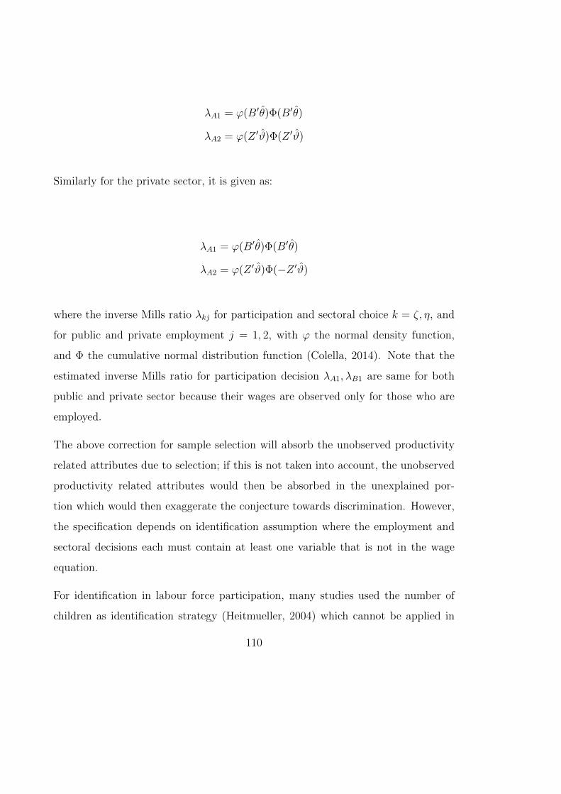
λA1 = ϕ(B′θ)Φ(B′θ)
λA2 = ϕ(Z ′ϑ)Φ(Z ′ϑ)
Similarly for the private sector, it is given as:
λA1 = ϕ(B′θ)Φ(B′θ)
λA2 = ϕ(Z ′ϑ)Φ(−Z ′ϑ)
where the inverse Mills ratio λkj for participation and sectoral choice k = ζ, η, and
for public and private employment j = 1, 2, with ϕ the normal density function,
and Φ the cumulative normal distribution function (Colella, 2014). Note that the
estimated inverse Mills ratio for participation decision λA1, λB1 are same for both
public and private sector because their wages are observed only for those who are
employed.
The above correction for sample selection will absorb the unobserved productivity
related attributes due to selection; if this is not taken into account, the unobserved
productivity related attributes would then be absorbed in the unexplained por-
tion which would then exaggerate the conjecture towards discrimination. However,
the specification depends on identification assumption where the employment and
sectoral decisions each must contain at least one variable that is not in the wage
equation.
For identification in labour force participation, many studies used the number of
children as identification strategy (Heitmueller, 2004) which cannot be applied in
110

our case, since we are observing male and female graduates who have invested in
education to increase their human capital in order to gain employment and earning.
Moreover, our sample graduates are rather homogenous among youth, and the in-
cidence of having a child would be very little. Instead, we observe graduates who
have some part time working experience during their study (i.e. semester break
temporary jobs or part time jobs while studying) and we found that those who have
some working experience by the time they graduated are more likely to be employed
regardless of the quality of the job they had. Their part time job during study is
however do not affect their subsequent job in the wage equation and thus making
this variable fit to be used as identification.
On the hand, identification in the sectoral decision is more complicated and depends
on country specific criteria. In the case of Malaysia, we would expect increased par-
ticipation in the public sector labour market among graduates whose parents are
or have worked with the public sector. Since we do not observed parent’s occupa-
tion, instead, we observe graduates who are already attached with a public sector
employer. They are sponsored by these employers1 with the expectation that after
study they return to work at the said employers. These graduates have obvious
tendency towards working with the sponsoring public sector employers. Thus, we
use this information as the identification strategy for sectoral choice.
Given the above construct, consistent estimate can be achieved. First, the partici-
pation and sectoral choice are estimated to obtain the inverse Mills ratio. Assum-
ing normal distribution of the error term, equation 3.5 can be estimated by the
Maximum Likelihood (MLE). Then the sample selection corrections factors are con-
structed and are used to estimate equation 3.1 for public/private (two equations) via
ordinal probit, including the inverse Mills ratio as additional regressor. The inverse
1Department of Public Services, the Ministry of Education, the Ministry of Health, and publicuniversities.
111
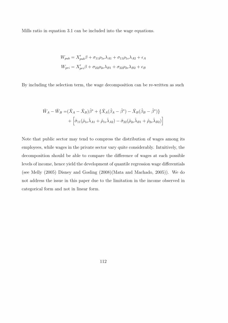
Mills ratio in equation 3.1 can be included into the wage equations.
Wpub = X ′pubβ + σ11ρ1νλA1 + σ11ρ1vλA2 + εA
Wpri = X ′priβ + σ22ρ2νλB1 + σ22ρ2vλB2 + εB
By including the selection term, the wage decomposition can be re-written as such
WA − WB =(XA − XB)β∗ + {XA(βA − β∗)− XB(βB − β∗)}
+[σ11(ρ1νλA1 + ρ1vλA2)− σ22(ρ2νλB1 + ρ2vλB2)
]
Note that public sector may tend to compress the distribution of wages among its
employees, while wages in the private sector vary quite considerably. Intuitively, the
decomposition should be able to compare the difference of wages at each possible
levels of income, hence yield the development of quantile regression wage differentials
(see Melly (2005) Disney and Gosling (2008)(Mata and Machado, 2005)). We do
not address the issue in this paper due to the limitation in the income observed in
categorical form and not in linear form.
112
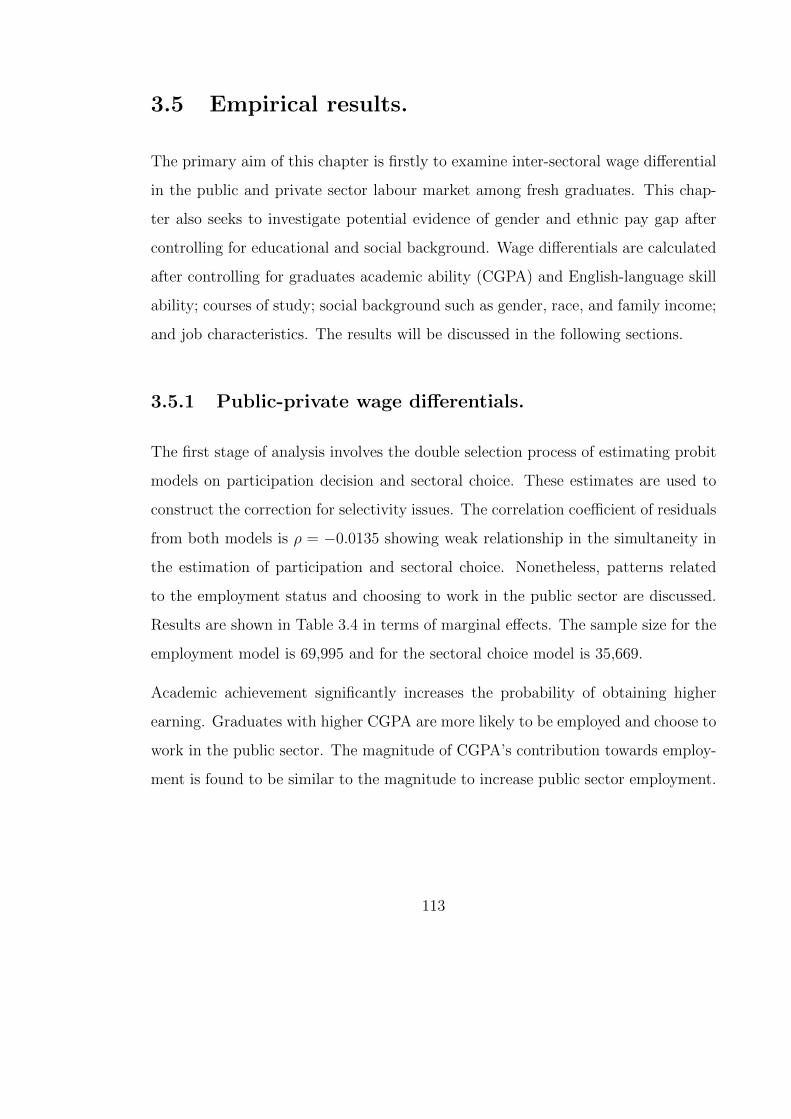
3.5 Empirical results.
The primary aim of this chapter is firstly to examine inter-sectoral wage differential
in the public and private sector labour market among fresh graduates. This chap-
ter also seeks to investigate potential evidence of gender and ethnic pay gap after
controlling for educational and social background. Wage differentials are calculated
after controlling for graduates academic ability (CGPA) and English-language skill
ability; courses of study; social background such as gender, race, and family income;
and job characteristics. The results will be discussed in the following sections.
3.5.1 Public-private wage differentials.
The first stage of analysis involves the double selection process of estimating probit
models on participation decision and sectoral choice. These estimates are used to
construct the correction for selectivity issues. The correlation coefficient of residuals
from both models is ρ = −0.0135 showing weak relationship in the simultaneity in
the estimation of participation and sectoral choice. Nonetheless, patterns related
to the employment status and choosing to work in the public sector are discussed.
Results are shown in Table 3.4 in terms of marginal effects. The sample size for the
employment model is 69,995 and for the sectoral choice model is 35,669.
Academic achievement significantly increases the probability of obtaining higher
earning. Graduates with higher CGPA are more likely to be employed and choose to
work in the public sector. The magnitude of CGPA’s contribution towards employ-
ment is found to be similar to the magnitude to increase public sector employment.
113

Table 3.4: Estimation results of participation choice and pub-lic sector employment (marginal effects).
(1) (2)Employed Public sector
Coef. s.e. Coef. s.e.
CGPA 0.105∗∗∗ (0.0143) 0.108∗∗∗ (0.0307)Arts/SocSc -0.176∗∗∗ (0.0456) 0.784∗∗∗ (0.101)Transport 0.408∗∗∗ (0.0938) 0.198 (0.187)Administration 0.208∗∗∗ (0.0452) 0.412∗∗∗ (0.102)Management 0.0626 (0.0434) 0.580∗∗∗ (0.0982)Economy 0.00316 (0.0521) 0.492∗∗∗ (0.115)Accountancy 0.377∗∗∗ (0.0453) -0.00732 (0.105)Marketing -0.0555 (0.0535) 0.295∗ (0.126)Finance 0.0898 (0.0463) 0.266∗ (0.106)Journalism -0.0341 (0.0509) 0.411∗∗∗ (0.111)Islamic 0.121∗ (0.0579) 0.921∗∗∗ (0.112)Food/hospitality 0.103 (0.0532) 0.274∗ (0.121)Arts -0.171∗∗∗ (0.0506) 0.196 (0.115)Pure science -0.170∗∗ (0.0560) 0.872∗∗∗ (0.115)Applied science -0.150∗∗∗ (0.0450) 0.646∗∗∗ (0.101)Pharmacy -0.484∗∗∗ (0.0757) 1.799∗∗∗ (0.146)Medical 0.526∗∗∗ (0.0529) 2.537∗∗∗ (0.108)Dentistry -0.330∗∗ (0.105) 3.001∗∗∗ (0.247)Nurse -0.0126 (0.0546) 0.348∗∗ (0.118)Environment -0.0646 (0.0530) 0.656∗∗∗ (0.114)Sports -0.222∗∗ (0.0822) 0.608∗∗∗ (0.166)Engineering 0.0622 (0.0418) -0.0563 (0.0968)CompSci 0.197∗∗∗ (0.0445) 0.277∗∗ (0.100)Education -0.349∗∗∗ (0.0453) 0.985∗∗∗ (0.100)Male 0.0623∗∗∗ (0.0107) -0.0871∗∗∗ (0.0220)Age 0.0978∗∗∗ (0.00499) 0.0737∗∗∗ (0.0105)Malay -0.00247 (0.0164) 0.101∗∗ (0.0338)Chinese 0.275∗∗∗ (0.0190) -0.255∗∗∗ (0.0400)RM 501 - RM 1000 0.0882∗∗∗ (0.0213) -0.0234 (0.0458)RM 1001 - RM 1500 0.145∗∗∗ (0.0219) 0.0375 (0.0466)RM 1501 - RM 2000 0.200∗∗∗ (0.0226) 0.00658 (0.0483)RM 2001 - RM 2500 0.184∗∗∗ (0.0240) 0.0432 (0.0508)RM 2501 - RM 3000 0.175∗∗∗ (0.0227) 0.0347 (0.0486)RM 3001 - RM 5000 0.141∗∗∗ (0.0224) 0.0489 (0.0479)> RM 5000 0.150∗∗∗ (0.0242) 0.0638 (0.0505)Urban 0.300∗∗∗ (0.0107) -0.114∗∗∗ (0.0214)Experiencea 0.278∗∗∗ (0.0103)
114
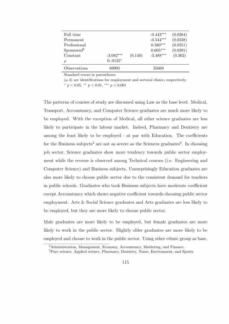
Full time -0.443∗∗∗ (0.0264)Permanent -0.544∗∗∗ (0.0238)Professional 0.380∗∗∗ (0.0251)Sponsoredb 0.605∗∗∗ (0.0391)Constant -3.082∗∗∗ (0.140) -3.488∗∗∗ (0.302)ρ 0-.0135∗
Observations 69995 35669
Standard errors in parentheses
(a, b) are identifications for employment and sectoral choice, respectively.∗ p < 0.05, ∗∗ p < 0.01, ∗∗∗ p < 0.001
The patterns of courses of study are discussed using Law as the base level. Medical,
Transport, Accountancy, and Computer Science graduates are much more likely to
be employed. With the exception of Medical, all other science graduates are less
likely to participate in the labour market. Indeed, Pharmacy and Dentistry are
among the least likely to be employed - at par with Education. The coefficients
for the Business subjects2 are not as severe as the Sciences graduates3. In choosing
job sector, Science graduates show more tendency towards public sector employ-
ment while the reverse is observed among Technical courses (i.e. Engineering and
Computer Science) and Business subjects. Unsurprisingly Education graduates are
also more likely to choose public sector due to the consistent demand for teachers
in public schools. Graduates who took Business subjects have moderate coefficient
except Accountancy which shows negative coefficient towards choosing public sector
employment. Arts & Social Science graduates and Arts graduates are less likely to
be employed, but they are more likely to choose public sector.
Male graduates are more likely to be employed, but female graduates are more
likely to work in the public sector. Slightly older graduates are more likely to be
employed and choose to work in the public sector. Using other ethnic group as base,
2Administration, Management, Economy, Accountancy, Marketing, and Finance.3Pure science, Applied science, Pharmacy, Dentistry, Nurse, Environment, and Sports.
115

Malay coefficient is not significantly different than the other ethnic in their labour
market participation but Malays are more likely to choose public sector employment.
Chinese is more likely to be employed, but less likely to work in the public sector
compared to the other ethnic group. Higher family income is associated with greater
probability to be employed. The magnitude is especially high among graduates with
moderate family income (RM1,500 - RM3,000). However, family income does not
affect the probability to choose public sector employment. Originating from an
urban state increases graduate’s employment probability due to the availability of
suitable jobs offered in the urban states - but urban graduates are less likely to work
in the public sector compared to non-urban graduates. Graduates who attended
public university are less likely to be employed but more likely to choose public
sector.
Graduates’ experience of part time jobs during study is used as the identification
for labour force participation estimation. The coefficient is positive and significant,
which indicates that these graduates are more employable than those who did not
have a part time or temporary job during or before study. Other the other hand,
graduates who were employed or attached with a public sector employer4 before or
during their study are naturally more likely to work with the public sector.
Job characteristics such as full time employment, permanent position, and profes-
sional jobs are used as controls in the sectoral choice model. Full time employment
and permanent position are negatively associated with public sector employment
but public sector workers are more likely to have professional jobs.
4Department of Public Services, the Ministry of Education, the Ministry of Health, and varioushigher learning institutions.
116
Separate public and private wage equations.
The second step involves the estimation of separate wage equation for public and
private sector by including the inverse Mills ratio as the correction for selectivity is-
sues. The response variable for the ordinal logit is eight incremental monthly income
level observed in Ringgit Malaysia. The marginal effects for the public and private
sector wage equations are given in Tables 3.5 and 3.6. The sample size for public
sector workers is 3,954 and private sector workers is 24,616. The overall pattern
shows that the determinants that led to better occupational category in the previ-
ous chapter also lead to higher income. Generally, graduates who performed better
academically, have better English proficiency, and took more attractive courses of
study are rewarded more. Detailed analysis of earning found that entry level earning
between public and private sectors is not significantly different, but men may earn
more in the private sector while Malays may earn more in the public sector. Higher
earners in the public sector generally have higher CGPA, indicating that graduates
with better academic achievement may seek public sector employment for its mon-
etary reward. English language is not an important element in the public sector
earning determination. Business subjects are rewarded more in the private sector,
while graduates who took Sciences subjects, Arts and Social Sciences may earn more
if they work in the public sector. More detailed analysis is further discussed.
Higher academic achievement increases the probability for higher income. For both
sectors, graduates with higher CGPA tend to earn more. The mean CGPA for pub-
lic and private sector workers are (3.40, 3.12) respectively. A one unit increase in
CGPA may additively increases public sector worker’s earning by 1.14 percentage
point to earn between RM1,001 - RM1,500 but decreases private sector worker’s
earning by 1.9 percentage point for the same income band. Higher CGPA increases
the probability for higher earning in the public sector starting from an income level of
117

RM1,000 but for private sector the positive effect of CGPA is observed at RM2,000.
Employers use CGPA to rank candidates and they are more likely to hire gradu-
ates with better grades considering academic performance can be easily observed to
indicate innate ability, commitment, and potential productive characteristics. The
estimation result shows evidence of wage premium among those with higher CGPA,
after controlling for other factors in consideration including courses of study.
Local studies on Malaysian graduate unemployment often cited graduate’s inability
to use English proficiently lead to unsuccessful job interviews (Devadason et. al.,
2010),(Ismail, 2011). This is especially true among graduates from public univer-
sities and rural female Malay graduates (Ismail, 2011). Apart from the interview
process to assess graduate’s English proficiency, MUET score can also be used dur-
ing a screening process even before the interview take place. Much as the same way
the CGPA is used to indicate potential ability, MUET score is used to demonstrate
English language ability. The results show that MUET is only positively associ-
ated with earning in the private sector, in view of the fact that English is the main
language in business and private practices and hence requirement for good English
proficiency is an essential factor during recruitment. However, MUET is only sig-
nificant between the middle score (Band 3 - 5) and its positive effect is detected
starting at the income level of RM2,000. MUET score is barely significant in the
public sector wage equation.
118

Tab
le3.5
:E
stim
ati
on
resu
lts
of
gra
du
ate
earn
ings
inth
ep
ub
lic
sect
or
emplo
ym
ent
(1)
(2)
(3)
(4)
(5)
(6)
(7)
(8)
CG
PA
-0.0
250∗
∗-0
.0467∗∗
0.0
114∗
∗0.0
231∗
∗0.0
118∗
∗0.0
0163
0.0
161∗
∗0.0
0775∗∗
Ban
d2
-0.0
00563
-0.0
00999
0.0
00283
0.0
00494
0.0
00233
0.0
0000419
0.0
00411
0.0
00136
Ban
d3
-0.0
0540
-0.0
100
0.0
0255
0.0
0493
0.0
0241
0.0
00153
0.0
0398
0.0
0142
Ban
d4
-0.0
104
-0.0
204
0.0
0449
0.0
0993
0.0
0504
0.0
00562
0.0
0774
0.0
0299
Ban
d5
-0.0
178∗
-0.0
376
0.0
0626∗
0.0
181∗
0.0
0978
0.0
0181
0.0
134
0.0
0593
Ban
d6
-0.0
133
-0.0
268
0.0
0536
0.0
130
0.0
0675
0.0
00943
0.0
0993
0.0
0404
Art
s/S
ocS
c-0
.187
-0.0
796
0.0
925∗
∗0.0
764∗
∗∗0.0
439∗
∗∗0.0
311∗
∗0.0
223∗
0.0
00330
Tra
nsp
ort
0.0
576
-0.0
0863
-0.0
237
-0.0
133
-0.0
0611
-0.0
0372
-0.0
0210
-0.0
000239
Ad
min
istr
atio
n-0
.110
-0.0
155
0.0
517
0.0
353
0.0
183
0.0
120
0.0
0772
0.0
000988
Man
agem
ent
-0.1
67
-0.0
560
0.0
824∗
0.0
637∗
∗0.0
355∗
∗∗0.0
245∗
∗∗0.0
170∗
∗0.0
00239∗
Eco
nom
y-0
.177
-0.0
669
0.0
875∗
∗0.0
698∗
∗0.0
395∗
∗∗0.0
275∗∗
0.0
194∗
∗0.0
00280∗
Acc
ounta
ncy
-0.0
728
-0.0
0391
0.0
333
0.0
215
0.0
108
0.0
0690
0.0
0428
0.0
000528
Mar
keti
ng
-0.1
10
-0.0
157
0.0
519
0.0
355
0.0
184
0.0
121
0.0
0777
0.0
000996
Fin
ance
-0.0
845
-0.0
0670
0.0
390
0.0
256
0.0
129
0.0
0836
0.0
0524
0.0
000653
Jou
rnal
ism
-0.1
57
-0.0
459
0.0
768∗
0.0
577∗
∗0.0
317∗
∗0.0
216∗∗
0.0
147∗
∗0.0
00203∗
Isla
mic
-0.1
83
-0.0
745
0.0
906∗
∗0.0
737∗
∗0.0
421∗
∗0.0
296∗
0.0
211∗
0.0
00309
Food
/hos
pit
alit
y-0
.0824
-0.0
0614
0.0
379
0.0
248
0.0
125
0.0
0808
0.0
0506
0.0
000629
Art
s-0
.0120
0.0
00681
0.0
0522
0.0
0314
0.0
0150
0.0
00936
0.0
00553
0.0
0000651
Pu
resc
ien
ce-0
.180
-0.0
712
0.0
893∗
0.0
720∗
∗0.0
410∗
∗0.0
287∗
∗0.0
204∗
0.0
00296
Ap
pli
edsc
ien
ce-0
.163
-0.0
520
0.0
802∗
0.0
614∗
∗0.0
340∗
∗0.0
233∗
∗0.0
161∗
0.0
00224
Ph
arm
acy
-0.2
74∗
-0.3
83∗∗
∗-0
.115
0.0
819
0.1
47∗∗
∗0.1
96∗∗
∗0.3
28∗
∗∗0.0
196
Med
ical
-0.2
76∗
-0.4
02∗∗
∗-0
.194∗
∗∗-0
.0683∗∗
-0.0
133
0.0
358
0.6
38∗∗
∗0.2
79∗
Den
tist
ry-0
.276∗
-0.4
02∗∗
∗-0
.193∗
∗∗-0
.0648∗∗
-0.0
0548
0.0
567
0.6
61∗
∗∗0.2
23
Nu
rse
-0.1
32
-0.0
275
0.0
637
0.0
453
0.0
241∗
0.0
161
0.0
106
0.0
00140
Envir
onm
ent
-0.1
80
-0.0
702
0.0
889∗∗
0.0
715∗
∗∗0.0
406∗
∗∗0.0
284∗
∗∗0.0
201∗
∗0.0
00292∗
Sp
orts
-0.1
94
-0.0
909
0.0
962∗
0.0
819∗
∗0.0
478∗
0.0
342∗
0.0
249
0.0
00377
En
gin
eeri
ng
0.0
422
-0.0
0555
-0.0
176
-0.0
100
-0.0
0463
-0.0
0283
-0.0
0161
-0.0
000185
Com
pS
ci-0
.0974
-0.0
107
0.0
455
0.0
305
0.0
156
0.0
101
0.0
0644
0.0
000814
Ed
uca
tion
-0.1
91
-0.0
855
0.0
945∗
0.0
793∗
∗0.0
460∗
∗0.0
327∗
0.0
237
0.0
00354
119

Mal
e-0
.00866
-0.0
162
0.0
0393
0.0
0799
0.0
0408
0.0
00563
0.0
0558
0.0
0268
Age
-0.0
193∗
∗-0
.0361∗∗
0.0
0879∗∗
0.0
179∗∗
0.0
0911∗∗
0.0
0126
0.0
125∗
∗0.0
059
9∗∗
Mal
ay-0
.0200∗
∗∗-0
.0374∗∗
∗0.0
0909∗
∗0.0
185∗∗
∗0.0
0943∗∗
∗0.0
0130∗
0.0
129∗
∗0.0
061
9∗∗
Ch
ines
e0.
00821
0.0
153
-0.0
0373
-0.0
0758
-0.0
0387
-0.0
00534
-0.0
0529
-0.0
0254
Familyincome
RM
501
-R
M10
00-0
.00612
-0.0
0854
0.0
0374
0.0
0442
0.0
0171
-0.0
00502
0.0
0432
0.0
00972
RM
1001
-R
M15
00-0
.0165
-0.0
255
0.0
0956
0.0
130
0.0
0545
-0.0
00911
0.0
119
0.0
0307
RM
1501
-R
M20
00-0
.0277
-0.0
477∗
0.0
143
0.0
239
0.0
110∗
-0.0
00352
0.0
202
0.0
0625∗
RM
2001
-R
M25
00-0
.0287
-0.0
500∗
0.0
146
0.0
251∗
0.0
116∗
-0.0
00225
0.0
210
0.0
0661∗
RM
2501
-R
M30
00-0
.0284∗
-0.0
494∗
0.0
145
0.0
248∗
0.0
115∗
-0.0
00258
0.0
208∗
0.0
0652∗
RM
3001
-R
M50
00-0
.0240
-0.0
398∗
0.0
130
0.0
201∗
0.0
0893∗
-0.0
00690
0.0
174
0.0
0505∗
>R
M50
00-0
.0407∗∗
-0.0
811∗∗
∗0.0
156∗
0.0
399∗
∗∗0.0
208∗
∗∗0.0
0276
0.0
305∗
∗0.0
123∗
∗∗
Urb
an0.
000457
0.0
00853
-0.0
00207
-0.0
00422
-0.0
00215
-0.0
000297
-0.0
00294
-0.0
00141
Fu
llti
me
-0.0
0824
-0.0
154
0.0
0374
0.0
0761
0.0
0388
0.0
00536
0.0
0531
0.0
0255
Per
man
ent
-0.0
158
-0.0
294
0.0
0716
0.0
146
0.0
0743
0.0
0103
0.0
102
0.0
0488
Pro
fess
ion
al-0
.109∗
∗∗-0
.204∗
∗∗0.0
497∗
∗∗0.1
01∗∗
∗0.0
516∗
∗∗0.0
0712∗
0.0
705∗
∗∗0.0
339∗
∗∗
λA
-0.0
198
-0.0
371
0.0
0901
0.0
183
0.0
0935
0.0
0129
0.0
128
0.0
0614
λB
-0.1
62∗
∗∗-0
.303∗
∗∗0.0
737∗
∗∗0.1
50∗∗
∗0.0
765∗
∗∗0.0
106∗
0.1
05∗∗
∗0.0
502∗
∗∗
Ob
serv
atio
ns
3954
3954
3954
3954
3954
3954
3954
395
4
Sta
nd
ard
erro
rsin
par
enth
eses
∗p<
0.05
,∗∗p<
0.01
,∗∗
∗p<
0.0
01
120

Tab
le3.6
:E
stim
ati
on
resu
lts
of
gra
du
ate
earn
ings
inth
ep
riva
tese
ctor
emplo
ym
ent
(1)
(2)
(3)
(4)
(5)
(6)
(7)
(8)
CG
PA
-0.0
157∗
∗∗-0
.0295∗∗
∗-0
.0199∗∗
∗-0
.00828∗∗
∗0.0
222∗
∗∗0.0
319∗∗
∗0.0
162∗
∗∗0.0
0315∗
∗∗
Ban
d2
0.00
0428
0.0
00790
0.0
00515
0.0
00146
-0.0
00672
-0.0
00800
-0.0
00346
-0.0
000615
Ban
d3
-0.0
0680∗
∗∗-0
.0131∗∗
∗-0
.00883∗
∗∗-0
.00331∗∗
∗0.0
106∗
∗∗0.0
139∗∗
∗0.0
0634∗∗
∗0.0
0115∗
∗∗
Ban
d4
-0.0
138∗
∗∗-0
.0278∗∗
∗-0
.0194∗∗
∗-0
.00905∗∗
∗0.0
211∗
∗∗0.0
310∗∗
∗0.0
151∗
∗∗0.0
0282∗
∗∗
Ban
d5
-0.0
188∗
∗∗-0
.0391∗∗
∗-0
.0279∗∗
∗-0
.0150∗∗
∗0.0
278∗
∗∗0.0
452∗∗
∗0.0
232∗
∗∗0.0
0447∗
∗∗
Ban
d6
0.00
224
0.0
0410
0.0
0265
0.0
00693
-0.0
0352
-0.0
0411
-0.0
0175
-0.0
00310
Art
s/S
ocS
c-0
.079
5∗∗
∗-0
.117∗∗
∗-0
.0572∗
∗∗0.0
237∗
∗0.1
06∗∗
∗0.0
859∗
∗∗0.0
322∗
∗∗0.0
0554∗
∗∗
Tra
nsp
ort
-0.0
313
-0.0
390
-0.0
117
0.0
203
0.0
352
0.0
198
0.00580
0.0
00901
Ad
min
istr
atio
n-0
.063
1∗∗∗
-0.0
871∗∗
∗-0
.0369∗∗
∗0.0
293∗
∗∗0.0
805∗
∗∗0.0
557∗
∗∗0.0
186∗
∗∗0.0
0304∗
∗∗
Man
agem
ent
-0.0
735∗∗
∗-0
.105∗∗
∗-0
.0490∗∗
∗0.0
270∗
∗∗0.0
967∗
∗∗0.0
734∗
∗∗0.0
262∗
∗∗0.0
0440∗
∗∗
Eco
nom
y-0
.079
2∗∗∗
-0.1
16∗∗
∗-0
.0568∗∗
∗0.0
240∗
∗∗0.1
06∗∗
∗0.0
853∗
∗∗0.0
319∗
∗∗0.0
0547∗
∗∗
Acc
ounta
ncy
-0.0
157
-0.0
187
-0.0
0456
0.0
110
0.0
165
0.0
0862
0.00243
0.0
00372
Mar
keti
ng
-0.0
869∗∗
∗-0
.132∗∗
∗-0
.0687∗∗
∗0.0
171∗
0.1
17∗∗
∗0.1
04∗∗
∗0.0
419∗
∗∗0.0
0746∗
∗∗
Fin
ance
-0.0
790∗
∗∗-0
.116∗∗
∗-0
.0565∗∗
∗0.0
241∗
∗∗0.1
05∗∗
∗0.0
849∗
∗∗0.0
317∗
∗∗0.0
0543∗
∗∗
Jou
rnal
ism
-0.0
868∗∗
∗-0
.132∗∗
∗-0
.0685∗∗
∗0.0
173∗
0.1
17∗∗
∗0.1
04∗∗
∗0.0
416∗
∗∗0.0
0742∗
∗∗
Isla
mic
0.02
87
0.0
300
0.0
0276
-0.0
220
-0.0
249
-0.0
112
-0.0
0294
-0.0
00441
Food
/hos
pit
alit
y-0
.033
5∗∗
∗-0
.0421∗∗
∗-0
.0131∗∗
∗0.0
215∗
∗0.0
381∗∗
∗0.0
217∗
∗∗0.0
0640∗∗
∗0.0
00997∗∗
∗
Art
s-0
.073
6∗∗
∗-0
.105∗∗
∗-0
.0491∗∗
∗0.0
270∗
∗∗0.0
968∗
∗∗0.0
736∗
∗∗0.0
263∗
∗∗0.0
0442∗
∗∗
Pu
resc
ien
ce-0
.089
2∗∗∗
-0.1
37∗∗
∗-0
.0727∗∗
∗0.0
143
0.1
20∗
∗∗0.1
11∗∗
∗0.0
457∗
∗∗0.0
0826∗
∗∗
Ap
pli
edsc
ien
ce-0
.089
9∗∗
∗-0
.139∗∗
∗-0
.0739∗∗
∗0.0
135
0.1
21∗
∗∗0.1
12∗∗
∗0.0
468∗
∗∗0.0
0849∗
∗∗
Ph
arm
acy
-0.0
457
-0.0
595
-0.0
212
0.0
266∗
∗0.0
545
0.0
333
0.0102
0.0
0162
Med
ical
-0.0
0116
-0.0
0133
-0.0
00256
0.0
00852
0.0
0114
0.0
00566
0.0
00155
0.0
000235
Den
tist
ry0.
0145
0.0
158
0.0
0220
-0.0
109
-0.0
133
-0.0
0626
-0.0
0167
-0.0
00252
Nu
rse
-0.0
846∗∗
∗-0
.127∗∗
∗-0
.0649∗∗
∗0.0
196∗
0.1
14∗∗
∗0.0
979∗
∗∗0.0
384∗
∗∗0.0
0677∗
∗∗
Envir
onm
ent
-0.0
805∗∗
∗-0
.119∗∗
∗-0
.0587∗∗
∗0.0
230∗
∗0.1
08∗∗
∗0.0
882∗
∗∗0.0
333∗
∗∗0.0
0575∗
∗∗
Sp
orts
-0.0
881∗∗
∗-0
.135∗∗
∗-0
.0708∗∗
∗0.0
157
0.1
19∗
∗∗0.1
07∗∗
∗0.0
438∗
∗∗0.0
0787∗
∗
En
gin
eeri
ng
-0.0
945∗
∗∗-0
.150∗∗
∗-0
.0827∗∗
∗0.0
0629
0.1
27∗
∗∗0.1
27∗∗
∗0.0
562∗
∗∗0.0
106∗∗
∗
Com
pS
ci-0
.083
6∗∗
∗-0
.125∗∗
∗-0
.0634∗∗
∗0.0
205∗
∗∗0.1
12∗∗
∗0.0
955∗
∗∗0.0
372∗
∗∗0.0
0651∗
∗∗
Ed
uca
tion
-0.0
813∗
∗∗-0
.120∗∗
∗-0
.0599∗∗
∗0.0
224∗
0.1
09∗∗
∗0.0
901∗
∗∗0.0
343∗
∗∗0.0
0594∗
∗
121
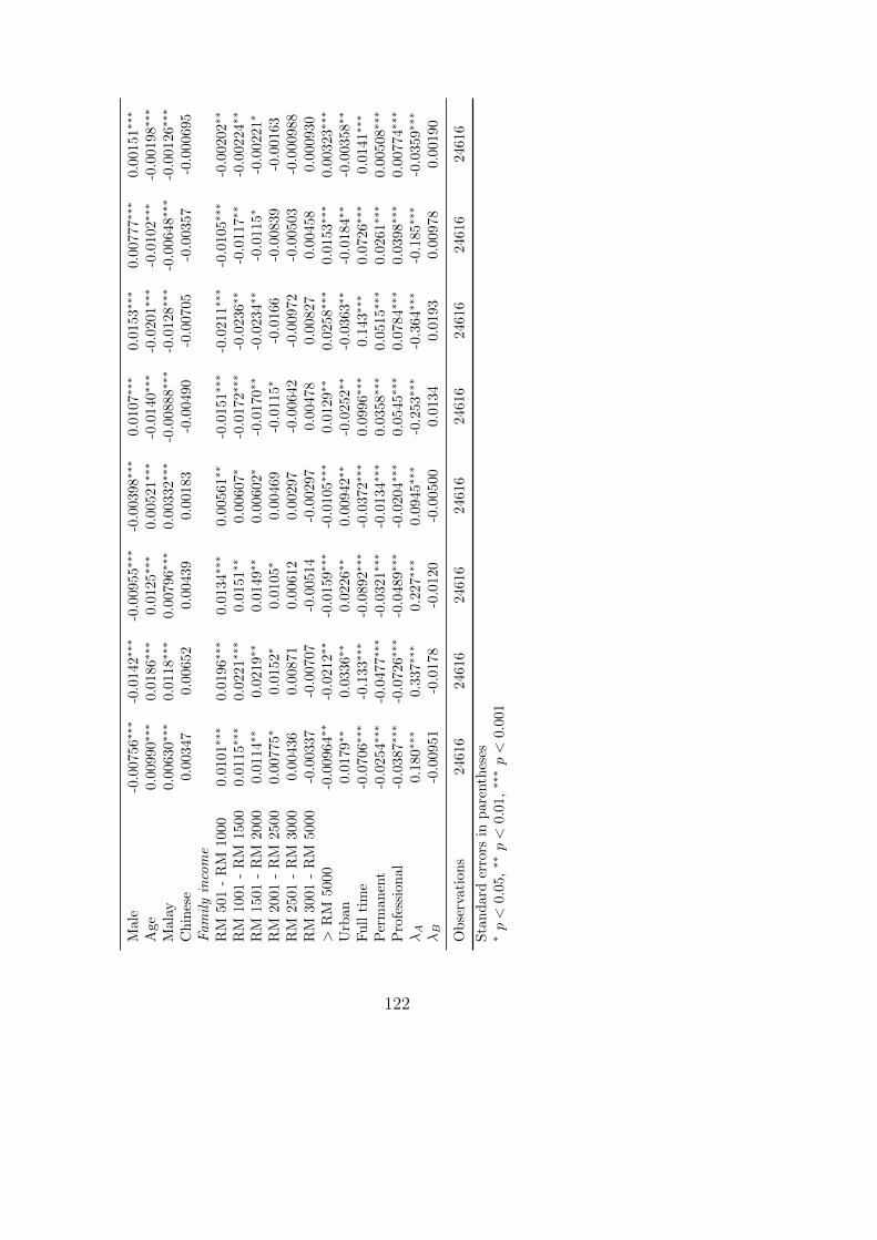
Mal
e-0
.007
56∗∗
∗-0
.0142∗∗
∗-0
.00955∗
∗∗-0
.00398∗∗
∗0.0
107∗
∗∗0.0
153∗
∗∗0.0
0777∗
∗∗0.0
0151∗∗
∗
Age
0.00
990∗
∗∗0.0
186∗∗
∗0.0
125∗
∗∗0.0
0521∗
∗∗-0
.0140∗∗
∗-0
.0201∗∗
∗-0
.0102∗∗
∗-0
.00198∗
∗∗
Mal
ay0.
0063
0∗∗∗
0.0
118∗∗
∗0.0
0796∗∗
∗0.0
0332∗
∗∗-0
.00888∗
∗∗-0
.0128∗∗
∗-0
.00648∗
∗∗-0
.00126∗
∗∗
Ch
ines
e0.
00347
0.0
0652
0.0
0439
0.0
0183
-0.0
0490
-0.0
0705
-0.0
0357
-0.0
00695
Familyincome
RM
501
-R
M10
000.
0101
∗∗∗
0.0
196∗∗
∗0.0
134∗
∗∗0.0
0561∗
∗-0
.0151∗∗
∗-0
.0211∗∗
∗-0
.0105∗∗
∗-0
.00202∗
∗
RM
1001
-R
M15
000.
0115
∗∗∗
0.0
221∗
∗∗0.0
151∗
∗0.0
0607∗
-0.0
172∗∗
∗-0
.0236∗∗
-0.0
117∗∗
-0.0
0224∗∗
RM
1501
-R
M20
000.
0114∗
∗0.0
219∗
∗0.0
149∗
∗0.0
0602∗
-0.0
170∗∗
-0.0
234∗∗
-0.0
115∗
-0.0
0221∗
RM
2001
-R
M25
000.
00775∗
0.0
152∗
0.0
105∗
0.0
0469
-0.0
115∗
-0.0
166
-0.0
0839
-0.0
0163
RM
2501
-R
M30
000.
00436
0.0
0871
0.0
0612
0.0
0297
-0.0
0642
-0.0
0972
-0.0
0503
-0.0
00988
RM
3001
-R
M50
00-0
.00337
-0.0
0707
-0.0
0514
-0.0
0297
0.0
0478
0.0
0827
0.0
0458
0.000930
>R
M50
00-0
.009
64∗∗
-0.0
212∗∗
-0.0
159∗∗
∗-0
.0105∗∗
∗0.0
129∗
∗0.0
258∗
∗∗0.0
153∗
∗∗0.0
0323∗∗
∗
Urb
an0.
0179∗
∗0.0
336∗
∗0.0
226∗
∗0.0
0942∗
∗-0
.0252∗∗
-0.0
363∗∗
-0.0
184∗∗
-0.0
0358∗
∗
Fu
llti
me
-0.0
706∗
∗∗-0
.133∗
∗∗-0
.0892∗∗
∗-0
.0372∗∗
∗0.0
996∗
∗∗0.1
43∗∗
∗0.0
726∗
∗∗0.0
141∗
∗∗
Per
man
ent
-0.0
254∗
∗∗-0
.0477∗∗
∗-0
.0321∗∗
∗-0
.0134∗∗
∗0.0
358∗
∗∗0.0
515∗
∗∗0.0
261∗
∗∗0.0
0508∗∗
∗
Pro
fess
ion
al-0
.038
7∗∗∗
-0.0
726∗∗
∗-0
.0489∗∗
∗-0
.0204∗∗
∗0.0
545∗
∗∗0.0
784∗
∗∗0.0
398∗
∗∗0.0
0774∗∗
∗
λA
0.18
0∗∗
∗0.3
37∗∗
∗0.2
27∗∗
∗0.0
945∗∗
∗-0
.253∗∗
∗-0
.364∗
∗∗-0
.185∗∗
∗-0
.0359∗∗
∗
λB
-0.0
0951
-0.0
178
-0.0
120
-0.0
0500
0.0
134
0.0
193
0.0
0978
0.0
0190
Ob
serv
atio
ns
2461
624616
24616
24616
24616
24616
24616
24616
Sta
nd
ard
erro
rsin
par
enth
eses
∗p<
0.05
,∗∗p<
0.01
,∗∗
∗p<
0.001
122
Male dummy coefficient is non-significant in the public sector wage equation, but
is positively associated with higher earnings in the private sector. The finding is
consistent with the public sector’s practice in maximising welfare, particularly in
providing similar wage structure regardless of gender. However, we do keep in
mind that male wage premium in the private sector may not be the evidence of
discrimination against women, instead, men higher earning in the private sector
may be due to their choice of more specialised and technical courses of study which
translate into higher earning because private sectors reward productivity. Female
graduates, on the other hand, who are generally associated with courses of study
that are related to low paying jobs - may earn better if they work in the public
sector instead of private sector. We will investigate the matter in greater details in
the subsequent analysis.
Slightly older graduates are associated with higher earning in the public sector, but
slightly younger graduates are associated with higher earning in the private sector.
Compared to the other ethnic group, Malays tend to earn more in the public sector
but tend to earn less in the private sector. Chinese coefficient in both sectors are
non-significant. Higher family income is barely significant in the public sector wage
equation, except for the highest family income group (>RM5,000) where graduates
from this family income level tend to earn higher in the public sector. The result
for family income is more mixed in the case of private sector wage equation. Using
the lowest family income level as the base, only the highest family income level
(>RM5,000) tend to earn more, while slightly higher family income from low to mid
income level (between RM501 - RM2,000) tend to earn less. The result may show
evidence that graduates with the lowest family income may perform well to increase
their intergenerational mobility.
Graduate originated from the urban states tend to earn less than the non-urban
123

graduates in the private sector indicating wage premium for non-urban who are
willing to migrate. The coefficient is non-significant in the public sector wage equa-
tion. Job characteristics such as full time employment and permanent position are
only significantly related to higher earning in the private sector, and non-significant
in the public sector considering public sector’s entry wage does not vary greatly.
Graduates with professional jobs tend to earn higher in both sectors. Finally, the
selection into employment is significant in the private sector wage equation, while
the selection into sectoral choice is significant in the public sector wage equation.
Coefficients for courses of study is given in the appendix on Table 3.16 and Ta-
ble 3.17. Using Law as the base category for courses of study, Arts and Social
Science course increases graduate’s probability for higher earning by 9.2 percentage
point in the public sector, while decreasing it by 5.7 percentage point in the private
sector. The positive effect of Art and Social Science course is observed starting
from RM1,500 for public sector employment, RM2,000 for private sector employ-
ment. However, the magnitude for higher income is large in the private sector for
these graduates. The overall results for other courses of study are quite mixed but
courses such as Management, Economy, Journalism, and Environment show similar
pattern. Several Business subjects (i.e. Management, Economy, Marketing, and Fi-
nance) show larger magnitude towards higher earning in the private sector. Islamic
study is only significant in the public sector. The effect of Pure and Applied Science
courses gave quite similar inter-sectoral pattern but the private sector workers have
higher tendency for higher earning. Pharmacy, Medical and Dentistry courses are
only significant in the public sector - which is not surprising because large majority
of them obtained jobs in the public sector. On the contrary, Nurse is only significant
in the private sector.
124

Decomposing public-private wage differential.
Using the results of the public and private wage equation presented earlier, the
inter-sectoral wage difference can be consistently estimated. Apart from calculat-
ing the mean wage difference between public and private sector and decomposing
them into several components, more meaningful result can be discussed based on
the contribution of explanatory variable towards the wage difference. However, the
computation of wage difference in based on the assumption of cardinality of the
graduate’s wage. This is because the computation of Oaxaca-Blinder (OB) decom-
position in a non-linear standard packages5 are only limited to the computation of
the average differences in the probability of earning especially in the case of an or-
dinal variable, restricting the computation of contribution from other explanatory
variables. The available packages also lack the ability to adjust for selectivity is-
sue. Therefore, we make assumption of the cardinality of the our response variable
and report the public-private decomposition analysis in Table 3.7. The assumption
of cardinality is supported by the fact that the wage indicator has cardinal mean-
ing: the change from the lowest category 1(<RM500) to the second lowest category
2(RM501 - RM1,000) has equivalent magnitude to the change from any of the subse-
quent wage indicator (a difference of RM500). The mid point within each category
has the same interval for all categories6.
The sample size n =28,570 is composed of both the public and private sector work-
ers. Column 2 of Table 3.7 reports the OB decomposition without considering the
issue of selectivity due to the sorting of graduates into employment and sectoral
choice, while column 4 reports the decomposition result after the adjustment in the
wage equation. The difference between the average probabilities between groups
5nldecompose,fairlie6Analysis based on the wage indicator (i.e. 1, 2, . . . , 8) has the same results as analysis based
on the wage mid-point (i.e. 750, 1250, . . . , 5250).
125

is computed from the wage equation, and the decomposition method compute part
that can be explained by the included variables and part that is due to the difference
between group A and B’s earning in the regression coefficients. For the Adjusted
part of the table, the average probabilities obtained by the separate wage equation
for public and private sectors are given by 0.635 and 0.763 respectively, with private
sector slightly higher by 12 percentage points. The difference (−0.128) composed
of the explained and unexplained components - the explained component (−0.176)
is the sum of all the contributing coefficients listed under the Explained part, while
the unexplained component (0.0487) is the sum of all the contributing coefficients
listed under the the Unexplained part. Out of the total difference of −0.128, 137%
of the difference is attributable to the Explained part while −38% is attributable
to the Unexplained part. The sum of contributing factors are larger under the Ex-
plained part, which signifies that the private sector’s higher earning due to their
better characteristics such as the choice of courses of study.
The average earning of public sector workers is found to be slightly lower than pri-
vate sector workers. Our preliminary result has some resemblance with the finding in
(Adamchik, 1999) who found that after controlling for characteristics and selection,
public sector pay less than private sector, especially among university graduates.
However in our case, the difference is not significant, both before and after adjust-
ment for selectivity. Unlike the previous study in Malaysia by Seshan (2013), we
cannot conclude the evidence of wage premium among public sector workers in our
sample. The result may be due to a homogenous sample of high skilled university
graduates who all possess tertiary education. Results for larger population as in Se-
shan (2013) may give different outcome (evidence for public sector wage premium).
Nonetheless, the difference is found to be accounted for by a mixed contribution
from the characteristic effects (the explained part) and the unexplained component.
Courses effect is negative indicating private sector workers generally possess quali-
126

fications that have high market value and it is rewarded in the private sectors. The
largest contribution towards the explained factor is job characteristics such as full
time employment and permanent job level. It is found that the proportion of private
sector workers in these occupational type is higher than the public sector but they
have lower proportion in professional jobs.
We next discuss the gender disparity in earning.
Table 3.7: Decomposition results for earning differentials in thepublic and private sector employment.
(1) (2)Unadjusted Adjusted
Coef. s.e.
DecompositionPublic 3.969∗∗∗ (0.0323) 3.969∗∗∗ (0.0323)Private 4.009∗∗∗ (0.00993) 4.009∗∗∗ (0.00993)Difference -0.0399 (0.0338) -0.0399 (0.0338)Explained -0.0296 (0.0283)Unexplained -0.0103 (0.0243)
AdjustedPublic 0.635 (0.374)Private 0.763∗∗∗ (0.129)Difference -0.128 (0.396)Explained -0.176 (0.0941)Unexplained 0.0487 (0.334)
ExplainedCGPA 0.0660∗∗∗ (0.00780) 0.0337∗∗∗ (0.00913)Muet 0.0184∗∗∗ (0.00347) 0.00983∗∗∗ (0.00277)Courses 0.119∗∗∗ (0.0182) -0.00369 (0.0680)Age 0.0139∗∗∗ (0.00226) -0.0147∗∗ (0.00460)Faminc 0.00150 (0.00251) 0.00984∗∗∗ (0.00225)Urban -0.0126∗∗∗ (0.00197) 0.0173∗∗∗ (0.00345)Full time -0.160∗∗∗ (0.00826) -0.160∗∗∗ (0.0104)Permanent -0.151∗∗∗ (0.00764) -0.144∗∗∗ (0.0122)Professional 0.0750∗∗∗ (0.00612) 0.0746∗∗∗ (0.00692)
UnexplainedCGPA -1.243∗∗∗ (0.201) -1.850∗∗∗ (0.242)Muet -0.136∗ (0.0687) -0.0305 (0.0680)Courses -0.674∗∗ (0.237) -1.726∗∗∗ (0.272)Age 2.111∗∗∗ (0.450) -2.102∗ (1.040)Faminc -0.0198 (0.0658) -0.106 (0.0756)
127

Urban -0.0493∗∗∗ (0.0135) -0.0566∗ (0.0284)Full time -0.242∗∗∗ (0.0343) 0.245∗∗∗ (0.0666)Permanent 0.140∗∗∗ (0.0193) 0.494∗∗∗ (0.0422)Professional -0.0245 (0.0296) -0.384∗∗∗ (0.0522)Constant 0.127 (0.571) 5.564∗∗∗ (1.207)
Observations 28570 28570
Standard errors in parentheses∗ p < 0.05, ∗∗ p < 0.01, ∗∗∗ p < 0.001
128

3.5.2 Gender pay gap.
Male-female wage equation.
In the previous chapter we showed that men and women graduates in our sample
have different first destination outcomes which men are found to be associated with
better occupational patterns compared to women. Better job category naturally
corresponds to higher pay, thus in this section we are investigating the source of
difference in men and women’s income controlling for various factors. To compute
the wage differential between men and women after controlling for their ability, socio-
economic status, and job attributes, the first step is to estimate the wage equation
separately for men and women. However, the wage equation lead to biased estimates
if the selection into employment is not taken into account. This may especially true
for women, since women are less likely to choose to participate into employment /
labour market, and more likely to choose lower paying job. However, for university
graduate we may expect the preference gap may reduce compared to women with
no higher education. We would expect women who spend longer time in education
would expect higher salary, perhaps similar to men. Since the wage equation for men
and especially women depend on some unobserved characteristics that lead them
into employment, we first construct a probit model for employment probability to
compute the inverse Mills ratio which is then included in wage equation to correct
for selection bias.
We discuss briefly the results of separate male-female wage equation. The marginal
effects of male and female wage equation is reported in Table 3.18 and 3.19 in the
appendix. The sample sizes are n = 10, 532 for male and n = 18, 038 for female .
Higher academic achievement increases earning for both sexes. The magnitude is
however, different - men is rewarded more for each unit increase in CGPA compared
to women. Proficiency in English is however only associated with higher earning
129
among female graduates. For male graduates, MUET score has barely significant
effect on earning. The overall pattern of the courses of study show that men gen-
erally have higher earning in comparison i.e. the magnitude of coefficient within
each course is higher for men than women for higher income groups. Transport,
Accountancy, Food & Hospitality courses only increase women’s probability to earn
higher but are not significant in the male wage equation. Compared to the other
ethnic group, only Malay male graduates show significant coefficient towards lower
earning. Chinese coefficient in the female wage equation is not significant implying
that the ethnicity does not play a role in the case of female wage. Hence, the effect
of ethnic group is only prevalent in the case of male graduates. Naturally, better
job characteristics are associated with higher earning for both gender groups.
Decomposition of gender pay gap.
Based on the above results, the decompositions of gender pay gap can be computed
and are reported in Table 3.8. The first three columns display the results for gender
pay gap in the pooled sample (column 1), among public sector workers (column
2), and among private sector workers (column 3). The unadjusted wage gap show
that male graduates consistently earn more in all the three model specifications.
After adjusting for participation into employment, only the private sector shows
persistent wage gap (men earn significantly higher by 92 percentage point in the
private sector with the difference due to the explained and unexplained components
is 31.4% and 68.6% respectively). The gap is largely due to the unexplained portion
of the wage differential, suggesting potential evidence of discrimination in the private
wage setting towards female graduates. Male significant higher earning in the private
sector can be attributable to their higher MUET score, the choice of courses of study,
and better job characteristics (men have higher proportion in full time employment,
permanent position, and professional jobs). The unexplained portion is due to the
130
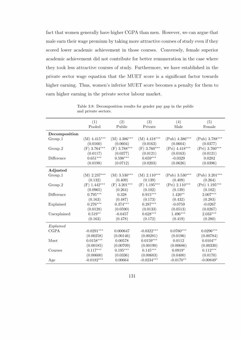
fact that women generally have higher CGPA than men. However, we can argue that
male earn their wage premium by taking more attractive courses of study even if they
scored lower academic achievement in those courses. Conversely, female superior
academic achievement did not contribute for better remuneration in the case where
they took less attractive courses of study. Furthermore, we have established in the
private sector wage equation that the MUET score is a significant factor towards
higher earning. Thus, women’s inferior MUET score becomes a penalty for them to
earn higher earning in the private sector labour market.
Table 3.8: Decomposition results for gender pay gap in the publicand private sectors.
(1) (2) (3) (4) (5)Pooled Public Private Male Female
DecompositionGroup 1 (M) 4.415∗∗∗ (M) 4.386∗∗∗ (M) 4.418∗∗∗ (Pub) 4.386∗∗∗ (Pub) 3.788∗∗∗
(0.0160) (0.0604) (0.0163) (0.0604) (0.0377)Group 2 (F) 3.764∗∗∗ (F) 3.788∗∗∗ (F) 3.760∗∗∗ (Pri) 4.418∗∗∗ (Pri) 3.760∗∗∗
(0.0117) (0.0377) (0.0121) (0.0163) (0.0121)Difference 0.651∗∗∗ 0.598∗∗∗ 0.659∗∗∗ -0.0329 0.0282
(0.0198) (0.0712) (0.0203) (0.0626) (0.0396)
AdjustedGroup 1 (M) 2.237∗∗∗ (M) 3.530∗∗∗ (M) 2.110∗∗∗ (Pub) 3.530∗∗∗ (Pub) 3.201∗∗∗
(0.132) (0.409) (0.139) (0.409) (0.264)Group 2 (F) 1.442∗∗∗ (F) 3.201∗∗∗ (F) 1.195∗∗∗ (Pri) 2.110∗∗∗ (Pri) 1.195∗∗∗
(0.0965) (0.264) (0.102) (0.139) (0.102)Difference 0.795∗∗∗ 0.328 0.915∗∗∗ 1.420∗∗ 2.007∗∗∗
(0.163) (0.487) (0.173) (0.432) (0.283)Explained 0.276∗∗∗ 0.374∗∗∗ 0.287∗∗∗ -0.0759 -0.0267
(0.0128) (0.0590) (0.0133) (0.0513) (0.0267)Unexplained 0.519∗∗ -0.0457 0.628∗∗∗ 1.496∗∗∗ 2.033∗∗∗
(0.163) (0.478) (0.172) (0.419) (0.280)
ExplainedCGPA -0.0291∗∗∗ 0.000647 -0.0322∗∗∗ 0.0760∗∗∗ 0.0296∗∗∗
(0.00258) (0.00146) (0.00281) (0.0196) (0.00784)Muet 0.0158∗∗∗ 0.00578 0.0159∗∗∗ 0.0112 0.0104∗∗
(0.00185) (0.00709) (0.00190) (0.00686) (0.00330)Courses 0.117∗∗∗ 0.195∗∗∗ 0.145∗∗∗ 0.0919∗ 0.112∗∗∗
(0.00600) (0.0336) (0.00683) (0.0400) (0.0170)Age -0.0182∗∗∗ 0.00664 -0.0234∗∗∗ -0.0170∗∗ -0.00849∗
131

(0.00207) (0.00416) (0.00255) (0.00558) (0.00335)Faminc 0.00995∗∗∗ 0.00490 0.0116∗∗∗ 0.00829 0.0109∗∗∗
(0.00196) (0.00397) (0.00222) (0.00490) (0.00262)Urban -0.00875∗∗∗ -0.00132 -0.00901∗∗∗ 0.0163∗∗ 0.0114∗∗∗
(0.00189) (0.00172) (0.00216) (0.00555) (0.00316)Full time 0.0337∗∗∗ 0.0425∗∗ 0.0229∗∗∗ -0.176∗∗∗ -0.150∗∗∗
(0.00514) (0.0142) (0.00532) (0.0173) (0.00925)Permanent 0.0424∗∗∗ 0.0889∗∗∗ 0.0303∗∗∗ -0.105∗∗∗ -0.152∗∗∗
(0.00357) (0.0147) (0.00326) (0.0115) (0.00922)Professional 0.113∗∗∗ 0.0312∗∗ 0.126∗∗∗ 0.0178 0.110∗∗∗
(0.00491) (0.0104) (0.00548) (0.00914) (0.00787)
UnexplainedCGPA 0.552∗∗∗ 0.0406 0.554∗∗∗ -0.997∗ -0.470
(0.136) (0.464) (0.141) (0.395) (0.251)Muet -0.158∗∗ 0.0875 -0.199∗∗∗ 0.138 -0.137
(0.0559) (0.135) (0.0604) (0.123) (0.0827)Courses -0.169 0.311 -0.199 -0.0907 -0.670∗
(0.123) (0.503) (0.127) (0.433) (0.282)Age -0.429 -1.929 0.103 3.951∗∗∗ 5.945∗∗∗
(0.443) (1.235) (0.471) (1.100) (0.728)Faminc 0.0920 0.0270 0.113 0.0973 0.187∗
(0.0549) (0.140) (0.0588) (0.128) (0.0818)Urban -0.000812 -0.0330 0.00747 0.0690 0.107∗∗∗
(0.0179) (0.0445) (0.0194) (0.0450) (0.0283)Full time 0.242∗∗∗ 0.287∗∗∗ 0.210∗∗∗ -0.142∗ -0.264∗∗∗
(0.0353) (0.0623) (0.0407) (0.0694) (0.0390)Permanent -0.0378∗ -0.0569 -0.0165 0.138∗∗∗ 0.167∗∗∗
(0.0149) (0.0305) (0.0166) (0.0375) (0.0223)Professional 0.0146 -0.0761 0.0306 -0.0915 0.0179
(0.0224) (0.0687) (0.0238) (0.0646) (0.0322)Constant 0.412 1.296 0.0230 -1.576 -2.849∗∗∗
(0.462) (1.328) (0.492) (1.189) (0.770)
Observations 28570 3954 24616 10532 18038
Standard errors in parentheses∗ p < 0.05, ∗∗ p < 0.01, ∗∗∗ p < 0.001
Column 4 and 5 of Table 3.8 shows the result for public-private wage differential
within each gender group. There is evidence of public pay premium for both gender,
with public pay premium among female graduates is larger than male. Courses of
study and job characteristics play major role in the explained part of the wage
differential. However, major contribution towards the pay premium is found to be
132

largely accounted for by the unexplained part of the wage differential which may
due to some unmeasured characteristics that are not included in the current model.
It may also due to some unexplained wage premium among public sector workers,
probably public sector’s better treatment towards low quality graduates.
133

Gender pay gap within different industry.
In the previous chapter we showed women are found to be under-represented in heav-
ily industrialised sectors associated with high skilled and high paying jobs (i.e. Con-
struction, Manufacturing, Scientific / Technical, IT / Communication, and Electric /
Gas / Steam). However, we are unable to conclude if women’s under-representation
in those sectors is due to taste or discrimination. In this section we are going to in-
vestigate if women who take up jobs in these industries face discrimination in terms
of lower wage than men. Perhaps if women earn significantly lower after controlling
for SES and education, any evidence of a gender wage gap may become an explana-
tion on why women may avoid seeking jobs in these sectors if their expected wage
does not compensate for their human capital in the same way as men.
The decomposition results for the gender differences within each industry are shown
in Tables 3.9-3.11. The adjusted decomposition results show that the gender gap
persists in Manufacturing, Food & Accommodation, and Defence. The large gen-
der gap in the Manufacturing industry where men earn significantly higher than
women shows that women employment and earning prospects in the Manufacturing
industry has not improved even when they have a degree qualification. Indeed, after
controlling for educational background and achievement, as well as graduates’ back-
ground and job characteristics, men-women pay gap in the Manufacturing industry
is still largely accounted for by the unexplained factor (96% of the total unexplained
part). Similar result is found in the Defence sector, where men have more preference
for higher earning. In contrast, women tend to earn more than men in the Food &
Accommodation. This industry is the third lowest paying industry in our sample,
while Manufacturing is the seventh higher paying industry.
134

Tab
le3.9
:D
ecom
posi
tion
resu
lts
for
gen
der
pay
gap
wit
hin
each
ind
ust
ry.
(1)
(2)
(3)
(4)
(5)
(6)
(7)
Agr
icu
ltu
re/
For
estr
y/
Fis
her
y
Min
ing
/Q
uarr
yM
anu
fact
uri
ng
Ele
ctri
c/
Gas
/S
team
Wate
r/
Sew
erage
Con
stru
ctio
nW
hole
sale
Dec
omp
osit
ion
Mal
e3.
657∗
∗∗5.6
90∗
∗∗4.8
29∗∗
∗4.8
11∗∗
∗4.3
65∗∗
∗4.8
35∗∗
∗3.1
84∗∗
∗
(0.1
14)
(0.1
55)
(0.0
358)
(0.0
957)
(0.2
13)
(0.0
375)
(0.0
814)
Fem
ale
3.25
0∗∗∗
4.8
10∗
∗∗4.1
34∗∗
∗4.4
45∗∗
∗3.8
63∗∗
∗4.3
16∗∗
∗2.6
40∗∗
∗
(0.0
960)
(0.1
82)
(0.0
348)
(0.1
19)
(0.1
53)
(0.0
356)
(0.0
416)
Diff
eren
ce0.
407∗
∗0.8
80∗∗
∗0.6
95∗∗
∗0.3
66∗
0.5
02
0.5
19∗∗
∗0.5
45∗∗
∗
(0.1
49)
(0.2
39)
(0.0
500)
(0.1
52)
(0.2
62)
(0.0
517)
(0.0
914)
Adjusted
Mal
e2.
122
4.0
05∗
∗3.0
49∗∗
∗3.0
22∗∗
∗3.0
01
1.7
27∗∗
∗-0
.888
(1.0
92)
(1.4
14)
(0.3
00)
(0.8
97)
(2.6
84)
(0.3
75)
(0.6
96)
Fem
ale
0.96
03.1
15
1.0
22∗
∗∗2.2
24
1.1
89
0.7
55∗
-1.0
56∗
∗
(0.8
99)
(1.7
12)
(0.2
71)
(1.1
77)
(1.3
22)
(0.3
62)
(0.3
85)
Diff
eren
ce1.
161
0.8
90
2.0
27∗
∗∗0.7
98
1.8
12
0.9
72
0.1
68
(1.4
15)
(2.2
20)
(0.4
05)
(1.4
80)
(2.9
92)
(0.5
21)
(0.7
96)
Exp
lain
ed-0
.088
00.6
24∗∗
0.3
64∗∗
∗0.3
69∗∗
0.2
92
0.1
40∗∗
∗0.0
843
(0.1
13)
(0.2
08)
(0.0
352)
(0.1
31)
(0.2
55)
(0.0
329)
(0.0
593)
Un
exp
lain
ed1.
249
0.2
66
1.6
62∗
∗∗0.4
29
1.5
21
0.8
32
0.0
841
(1.4
27)
(2.1
99)
(0.4
04)
(1.4
83)
(3.0
94)
(0.5
20)
(0.7
84)
Ob
serv
atio
ns
509
166
2987
477
125
2473
1224
tst
atis
tics
inp
aren
thes
es.
∗p<
0.05,∗∗p<
0.01,∗∗
∗p<
0.0
01
135

Tab
le3.1
0:
Dec
om
posi
tion
resu
lts
for
gen
der
pay
gap
wit
hin
each
ind
ust
ry.
(8)
(9)
(10)
(11)
(12)
(13)
(14)
Tra
nsp
ort
/S
tora
geF
ood
/A
ccom
.IT
/C
om
m.
Fin
an
ce/
Insu
ran
ceR
eal
esta
teS
cien
tifi
c/
Tec
hn
ical
Ad
min
/S
up
port
Decomposition
Mal
e4.
083∗
∗∗2.8
22∗∗
∗4.7
81∗∗
∗4.7
16∗∗
∗4.1
37∗∗
∗5.1
85∗∗
∗3.5
98∗∗
∗
(0.1
04)
(0.0
683)
(0.0
469)
(0.0
484)
(0.1
22)
(0.0
386)
(0.0
811)
Fem
ale
3.92
6∗∗
∗2.8
64∗∗
∗4.3
24∗∗
∗4.3
50∗∗
∗3.8
12∗∗
∗4.6
76∗∗
∗3.3
28∗∗
∗
(0.0
662)
(0.0
438)
(0.0
411)
(0.0
324)
(0.0
781)
(0.0
364)
(0.0
486)
Diff
eren
ce0.
157
-0.0
420
0.4
58∗
∗∗0.3
66∗∗
∗0.3
25∗
0.5
10∗∗
∗0.2
70∗∗
(0.1
24)
(0.0
812)
(0.0
623)
(0.0
583)
(0.1
44)
(0.0
531)
(0.0
945)
Adjusted
Mal
e1.
644
-2.1
51∗∗
2.8
21∗∗
∗3.0
76∗∗
∗0.6
10
3.6
57∗∗
∗2.1
95∗
(1.1
16)
(0.7
16)
(0.4
42)
(0.4
62)
(1.4
90)
(0.3
26)
(0.8
99)
Fem
ale
0.46
40.6
07
2.4
03∗
∗∗2.5
16∗∗
∗-1
.330
3.3
59∗
∗∗0.6
57
(0.6
21)
(0.4
01)
(0.3
84)
(0.3
13)
(0.7
50)
(0.2
80)
(0.5
50)
Diff
eren
ce1.
180
-2.7
57∗
∗∗0.4
18
0.5
60
1.9
40
0.2
99
1.5
39
(1.2
77)
(0.8
21)
(0.5
86)
(0.5
58)
(1.6
68)
(0.4
30)
(1.0
54)
Exp
lain
ed-0
.032
6-0
.106
0.2
20∗
∗∗0.1
35∗∗
∗-0
.00150
0.2
12∗
∗∗0.1
13
(0.0
760)
(0.0
565)
(0.0
404)
(0.0
361)
(0.0
959)
(0.0
374)
(0.0
596)
Un
exp
lain
ed1.
213
-2.6
51∗∗
0.1
99
0.4
25
1.9
42
0.0
863
1.4
26
(1.2
82)
(0.8
26)
(0.5
82)
(0.5
56)
(1.6
64)
(0.4
29)
(1.0
52)
Ob
serv
atio
ns
583
1193
2059
2521
452
3750
1093
tst
atis
tics
inp
aren
thes
es.
∗p<
0.05,∗∗p<
0.0
1,∗∗
∗p<
0.001
136
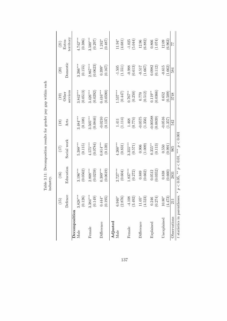
Tab
le3.1
1:
Dec
om
posi
tion
resu
lts
for
gen
der
pay
gap
wit
hin
each
ind
ust
ry.
(15)
(16)
(17)
(18)
(19)
(20)
(21)
Def
ence
Ed
uca
tion
Soci
al
work
Art
sO
ther
serv
ices
Dom
esti
cE
xtr
a-
terr
itory
Decomposition
Mal
e3.
828∗
∗∗3.1
96∗
∗∗5.3
88∗∗
∗3.4
84∗∗
∗3.8
42∗∗
∗3.2
66∗∗
∗4.7
42∗∗
∗
(0.1
26)
(0.0
562)
(0.1
15)
(0.1
08)
(0.0
513)
(0.1
55)
(0.3
86)
Fem
ale
3.38
4∗∗∗
2.8
08∗
∗∗4.5
75∗∗
∗3.5
05∗∗
∗3.4
26∗∗
∗2.8
67∗∗
∗3.5
00∗∗
∗
(0.1
49)
(0.0
259)
(0.0
784)
(0.0
846)
(0.0
292)
(0.0
623)
(0.2
97)
Diff
eren
ce0.
444∗
0.3
89∗∗
∗0.8
14∗∗
∗-0
.0210
0.4
16∗
∗∗0.3
99∗
1.2
42∗
(0.1
95)
(0.0
619)
(0.1
39)
(0.1
37)
(0.0
590)
(0.1
67)
(0.4
87)
Adjusted
Mal
e6.
940∗
2.7
27∗
∗∗4.2
60∗∗
∗1.4
11
1.5
37∗∗
∗-1
.505
11.9
4∗
(2.8
76)
(0.6
04)
(0.8
31)
(1.1
14)
(0.4
47)
(1.5
51)
(4.6
81)
Fem
ale
-4.1
081.8
37∗
∗∗3.3
55∗∗
∗1.4
68
0.7
67∗∗
-0.9
88
-1.0
25
(3.4
92)
(0.2
72)
(0.5
71)
(0.7
74)
(0.2
50)
(0.6
13)
(5.0
44)
Diff
eren
ce11
.05∗
0.8
89
0.9
06
-0.0
575
0.7
70
-0.5
17
12.9
6(4
.523
)(0
.662)
(1.0
09)
(1.3
56)
(0.5
12)
(1.6
67)
(6.8
82)
Exp
lain
ed0.
246
0.0
512
0.3
55∗
∗-0
.00588
0.1
19∗∗
0.0
982
0.8
66
(0.2
74)
(0.0
352)
(0.1
13)
(0.0
839)
(0.0
366)
(0.1
12)
(1.0
74)
Un
exp
lain
ed10
.80∗
0.8
38
0.5
50
-0.0
516
0.6
52
-0.6
15
12.0
9(4
.473
)(0
.660)
(0.9
91)
(1.3
57)
(0.5
09)
(1.6
62)
(6.9
63)
Ob
serv
atio
ns
211
2831
965
542
3748
584
77
tst
atis
tics
inp
aren
thes
es.
∗p<
0.05,∗∗p<
0.01,∗∗
∗p<
0.0
01
137

3.5.3 Wage differential by ethnic groups.
The ethnic wage differentials are computed between major ethnic groups in the
country - Malays, Chinese, and all the other ethnics which are classified into one
group due to large diversity and significantly lower representative proportion of the
smaller groups. We make separate analysis among public and private sector workers.
Table 3.12 reports the decomposition results for ethnic wage differential in the
public sector. Detailed source of difference is given in the appendix (Table 3.20).
The unadjusted wage difference is positive and significant between all groups, with
Chinese earning significantly higher than all the other groups combined, and other
ethnic group earn higher than Malays. The gap disappears however, after correcting
for selectivity issue. All the wage differences between all ethnic groups are now
insignificant. The result is consistent with public sector’s non-discriminatory policy
in the recruitment process. Nonetheless, the existence of the ethnic wage difference
in the public sector is found to be largely due to graduates’ characteristic effects.
Particularly, the course of study bear 50% contribution towards the explained part of
the wage difference. The other contributing factor are the type of job characteristics
possessed by those with higher earning.
Table 3.13 reports the ethnic wage differential in the private sector labour market.
Detailed source of difference is given in the appendix (Table 3.21). The unadjusted
wage differential shows similar result as in the unadjusted public sector outcome.
However, after adjusting for participation decision, ethnic wage gap in the private
sector is found to be persistent between Chinese and Malays, and between the other
ethnic group and Malays, with Malays consistently earn lower. Furthermore, the
ethnic wage differential in the private sector are largely accounted for by the unex-
plained part. 76% of the Chinese-Malay wage difference is due to the unexplained
part, while 89% of the wage difference between the other ethnic group and Malays
138
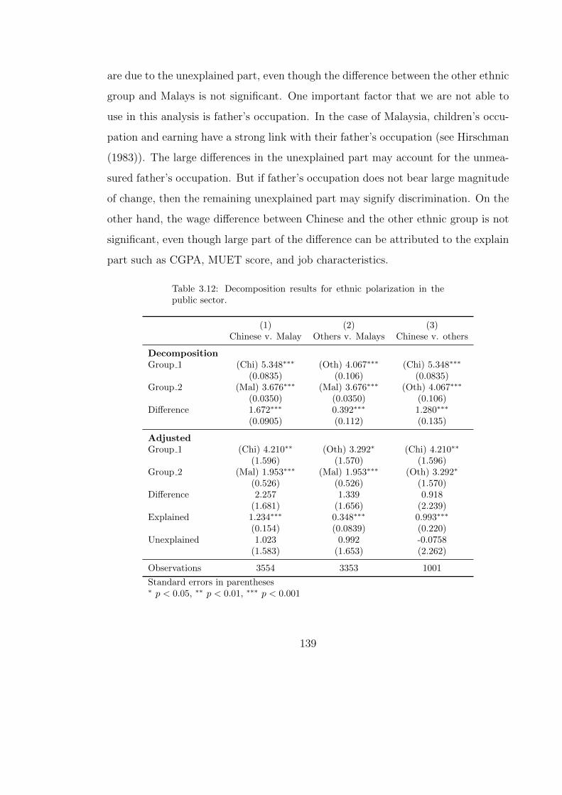
are due to the unexplained part, even though the difference between the other ethnic
group and Malays is not significant. One important factor that we are not able to
use in this analysis is father’s occupation. In the case of Malaysia, children’s occu-
pation and earning have a strong link with their father’s occupation (see Hirschman
(1983)). The large differences in the unexplained part may account for the unmea-
sured father’s occupation. But if father’s occupation does not bear large magnitude
of change, then the remaining unexplained part may signify discrimination. On the
other hand, the wage difference between Chinese and the other ethnic group is not
significant, even though large part of the difference can be attributed to the explain
part such as CGPA, MUET score, and job characteristics.
Table 3.12: Decomposition results for ethnic polarization in thepublic sector.
(1) (2) (3)Chinese v. Malay Others v. Malays Chinese v. others
DecompositionGroup 1 (Chi) 5.348∗∗∗ (Oth) 4.067∗∗∗ (Chi) 5.348∗∗∗
(0.0835) (0.106) (0.0835)Group 2 (Mal) 3.676∗∗∗ (Mal) 3.676∗∗∗ (Oth) 4.067∗∗∗
(0.0350) (0.0350) (0.106)Difference 1.672∗∗∗ 0.392∗∗∗ 1.280∗∗∗
(0.0905) (0.112) (0.135)
AdjustedGroup 1 (Chi) 4.210∗∗ (Oth) 3.292∗ (Chi) 4.210∗∗
(1.596) (1.570) (1.596)Group 2 (Mal) 1.953∗∗∗ (Mal) 1.953∗∗∗ (Oth) 3.292∗
(0.526) (0.526) (1.570)Difference 2.257 1.339 0.918
(1.681) (1.656) (2.239)Explained 1.234∗∗∗ 0.348∗∗∗ 0.993∗∗∗
(0.154) (0.0839) (0.220)Unexplained 1.023 0.992 -0.0758
(1.583) (1.653) (2.262)
Observations 3554 3353 1001
Standard errors in parentheses∗ p < 0.05, ∗∗ p < 0.01, ∗∗∗ p < 0.001
139
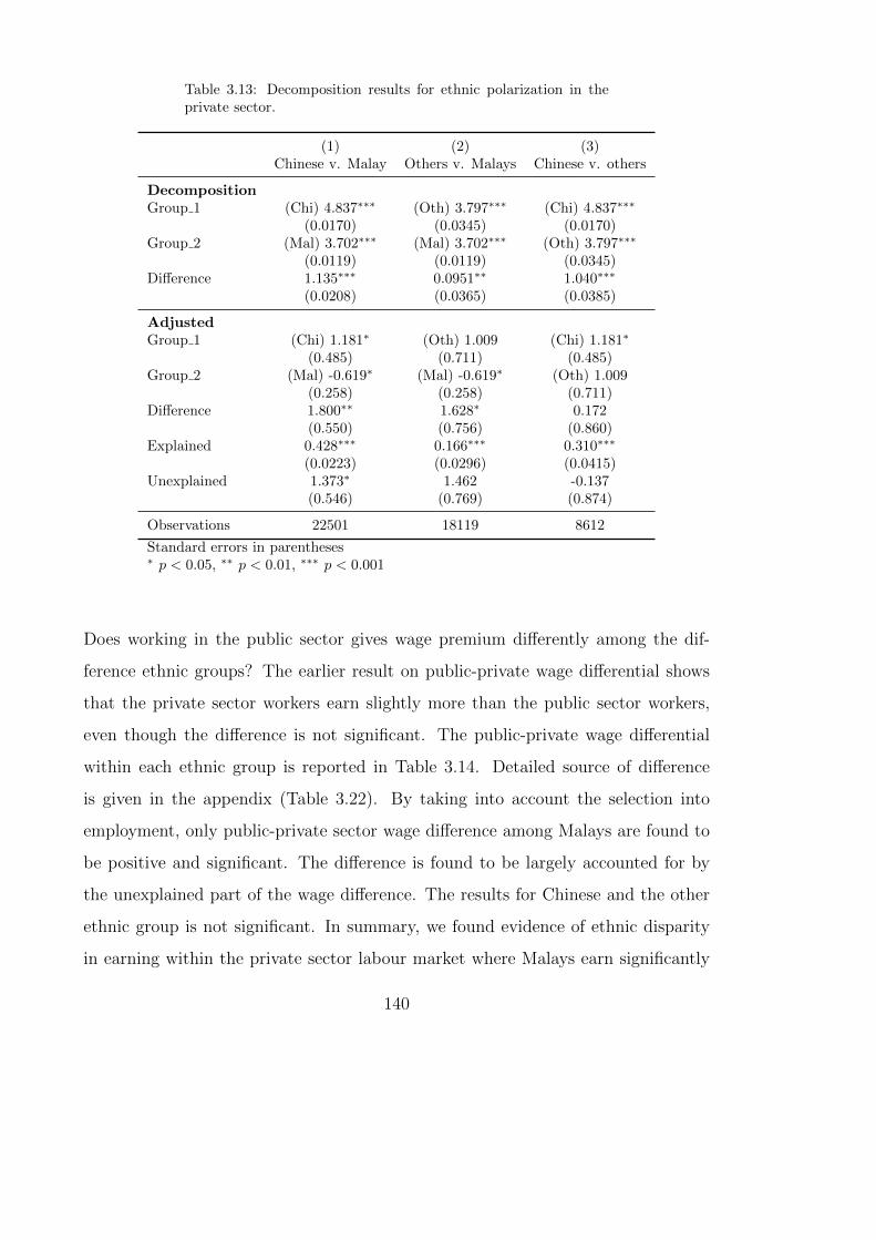
Table 3.13: Decomposition results for ethnic polarization in theprivate sector.
(1) (2) (3)Chinese v. Malay Others v. Malays Chinese v. others
DecompositionGroup 1 (Chi) 4.837∗∗∗ (Oth) 3.797∗∗∗ (Chi) 4.837∗∗∗
(0.0170) (0.0345) (0.0170)Group 2 (Mal) 3.702∗∗∗ (Mal) 3.702∗∗∗ (Oth) 3.797∗∗∗
(0.0119) (0.0119) (0.0345)Difference 1.135∗∗∗ 0.0951∗∗ 1.040∗∗∗
(0.0208) (0.0365) (0.0385)
AdjustedGroup 1 (Chi) 1.181∗ (Oth) 1.009 (Chi) 1.181∗
(0.485) (0.711) (0.485)Group 2 (Mal) -0.619∗ (Mal) -0.619∗ (Oth) 1.009
(0.258) (0.258) (0.711)Difference 1.800∗∗ 1.628∗ 0.172
(0.550) (0.756) (0.860)Explained 0.428∗∗∗ 0.166∗∗∗ 0.310∗∗∗
(0.0223) (0.0296) (0.0415)Unexplained 1.373∗ 1.462 -0.137
(0.546) (0.769) (0.874)
Observations 22501 18119 8612
Standard errors in parentheses∗ p < 0.05, ∗∗ p < 0.01, ∗∗∗ p < 0.001
Does working in the public sector gives wage premium differently among the dif-
ference ethnic groups? The earlier result on public-private wage differential shows
that the private sector workers earn slightly more than the public sector workers,
even though the difference is not significant. The public-private wage differential
within each ethnic group is reported in Table 3.14. Detailed source of difference
is given in the appendix (Table 3.22). By taking into account the selection into
employment, only public-private sector wage difference among Malays are found to
be positive and significant. The difference is found to be largely accounted for by
the unexplained part of the wage difference. The results for Chinese and the other
ethnic group is not significant. In summary, we found evidence of ethnic disparity
in earning within the private sector labour market where Malays earn significantly
140
lower than all the other ethnic groups. However, Malays may choose to work in the
public sector to improve their earning prospect even though there is no evidence that
the public sector practices ethnic-based recruitment by giving preferential treatment
to the Malays. This finding sparks another question on factors that cause Malay’s
inferior earning compared to the others having similar qualifications. We found
that Malays are slightly over-represented in less attractive courses such as Manage-
ment, Islamic studies, Education, and Arts (even though Malay are also found to
be slightly over-represented in Engineering). On the other spectrum, Chinese are
slightly over-represented in courses such as Computer Science, Accountancy, and
Administration (even though Chinese are also slightly over-represented in Market-
ing and Applied Science). However, course differences have been taken into account
in the decomposition of the Malay-Chinese wage gap. Hence, we would recommend
the study of Malay-Chinese persistent wage gap in the future research to gain a thor-
ough understanding, particularly by observing the influence of parental occupation
and education.
141

Table 3.14: Decomposition results for public-private earning differ-entials within each ethnic group.
(1) (2) (3)Malay Chinese Others
DecompositionPublic 3.676∗∗∗ 5.348∗∗∗ 4.067∗∗∗
(0.0350) (0.0835) (0.106)Private 3.702∗∗∗ 4.837∗∗∗ 3.797∗∗∗
(0.0119) (0.0170) (0.0345)Difference -0.0261 0.511∗∗∗ 0.271∗
(0.0370) (0.0852) (0.111)
AdjustedPublic 1.953∗∗∗ 4.210∗∗ 3.292∗
(0.526) (1.596) (1.570)Private -0.619∗ 1.181∗ 1.009
(0.258) (0.485) (0.711)Difference 2.572∗∗∗ 3.028 2.283
(0.586) (1.668) (1.723)Explained -0.0543∗ 0.00143 -0.0277
(0.0245) (0.125) (0.0868)Unexplained 2.626∗∗∗ 3.027 2.311
(0.585) (1.582) (1.695)
Observations 18957 7098 2515
Standard errors in parentheses∗ p < 0.05, ∗∗ p < 0.01, ∗∗∗ p < 0.001
142
3.5.4 Full time pay premium.
Table 3.15 shows the results for the wage differential between full time workers
and part time workers with detailed source of difference is given in the appendix
(Table 3.23). Consistent with our expectation, we found evidence of wage premium
among full time workers in our sample for both gender groups. In the case of male
graduates, 68% of the difference is due to the unexplained portion of the wage
difference. Full time workers among male graduates have higher CGPA, higher
family income, and higher probability for permanent position and professional jobs.
But the unexplained part is also largely due to the choice of courses of study. Wage
premium among female full time workers is not as big as male. Indeed, large and
significant portion of the wage difference is due to the explained part of the wage
difference (higher CGPA, higher MUET score, higher family income, and better job
characteristics).
Even though we found significant difference between full time - part time workers
among first degree graduates, but we do not expect that this will continue especially
because the survey is done within a very short period right after finishing study.
Some graduates, in particular those with part time jobs, may use the first job offer
as a stepping stone to gain experience before they begin their career. It would
be interesting to see the progress of part time workers over the years to test the
hypothesis if first job affect subsequent jobs. However, since we do not have the
tracer study data hence we keep this for future research.
143

Table 3.15: Decomposition results for earning differential be-tween full time / part time workers.
(1) (2) (3)Pooled Male Female
DecompositionFull time 4.358∗∗∗ 4.779∗∗∗ 4.104∗∗∗
(0.00973) (0.0152) (0.0122)Part time 2.298∗∗∗ 2.399∗∗∗ 2.249∗∗∗
(0.0155) (0.0295) (0.0181)Difference 2.060∗∗∗ 2.381∗∗∗ 1.855∗∗∗
(0.0183) (0.0332) (0.0218)
AdjustedFull time 1.766∗∗∗ 2.637∗∗∗ 1.646∗∗∗
(0.0781) (0.141) (0.106)Part time 0.672∗∗∗ 0.436 0.940∗∗∗
(0.182) (0.391) (0.237)Difference 1.094∗∗∗ 2.201∗∗∗ 0.706∗∗
(0.198) (0.416) (0.259)Explained 0.553∗∗∗ 0.685∗∗∗ 0.503∗∗∗
(0.0290) (0.0567) (0.0353)Unexplained 0.541∗ 1.516∗∗∗ 0.202
(0.213) (0.449) (0.278)
Observations 28570 10532 18038
Standard errors in parentheses∗ p < 0.05, ∗∗ p < 0.01, ∗∗∗ p < 0.001
144

3.6 Conclusion.
Previous studies in Malaysia have been focusing on graduate employability and
they generally criticize graduates for their lack of skills to fulfill the market demand.
Among the many issues is Malaysian graduate’s English language proficiency. Our
study shows that English plays an important role in obtaining a job and a high
income, but we found another key finding: the courses of study. Unemployment
is higher within certain courses of study. Malays and women generally have lower
labour force participation and lower earning, they are also found to have some
preference towards these less attractive courses.
In studying the public-private wage gap, we arrived at the conclusion that there
is no evidence of public sector wage premium among our graduates. The result is
different than the earlier finding in the country due to the different composition
of sample characteristics. Seshan (2013) found an evidence of public pay premium
in which the private sector in the country was found to be lagged behind in wage
determination that may lead to uncompetitiveness. The sample in our study is
composed of a group of high skilled workers who possess university qualification and
hence cannot be comparable to the larger population.
Due to the restriction in the type of response variable from the tracer study, we
cannot test for the existence of double imbalance in the distribution of the wage
distribution. Even though the private sector workers earn slightly higher than the
public sector workers, the difference is found to be non-significant. Higher earning
among private sector workers is largely due to their better choice of courses of
study. The connection between courses of study and sectors is also prevalent -
private sector restricts employee recruitment from those who took courses that have
higher private benefits such as Engineering, Management, and Accountancy; while
145

there is a higher proportion of public sector recruitment among graduates who took
Medical and Education.
Gender pay gap is only significant in the private sector labour market. The gap
is largely due to the unexplained part of the difference - female graduates have
higher CGPA but the superior academic achievement does not translate into better
remuneration in the private sector, hampered by their choice of less attractive courses
of study. Unlike the private sector, the public sector does not show evidence of gender
pay gap. Women in our study have a tendency to choose less attractive courses of
study that are usually associated with blurred employment prospect and low pay
compared to men’s preferences towards highly technical and attractive courses of
study. We found that even if women have similar qualification as men such as in
the case of Engineering, they still have lower earning. It is difficult to ascertain
the reason for Engineering women’s avoidance of getting a better job and higher
earning unless we have a suitable instrument to measure whether the difference is
due to their preference or discrimination. We also found evidence of gender pay
gap in industries such as Manufacturing and Defence (favouring males), and Food
& Accommodation (favouring females).
We found no evidence of pay differences among the different ethnic groups in the
public sector, nonetheless, the small wage difference is found to be associated with
the explained part of the wage gap, particularly, the choice of courses of study. The
opposite can be said about the private sector. We found evidence of significant
wage differential between all other ethnic groups and Malays, largely due to the
unexplained part. In studying wage differential between ethnic groups in Malaysia,
previous literatures showed that intergenerational inheritance in terms of father’s
occupations plays a very strong influential role in their children’s employment pat-
tern. Indeed, across all ethnic group, the intergenerational occupation inheritance
146

is a strong predictor of their offspring’s type of occupation and earning. However,
in the tracer study we do not have information on father’s occupation and hence
with the available data, we could not be able to make further investigation related
to the ethnic wage differential.
The increase in the number of Malay student intake into university does not help
to reduce ethnic inequality because they entered courses that do not alleviate their
economic status (most of them come from a rural area with low family income).
This finding sparks another question on factors that cause Malay’s inferior earn-
ing compared to the others having the same level of qualifications. We found that
Malays are slightly over-represented in less attractive courses such as Management,
Islamic studies, Education, and Arts (even though Malay are also found to be slightly
over-represented in Engineering). On the other spectrum, Chinese are slightly over-
represented in courses such as Medical, Computer Science, Accountancy, and Ad-
ministration (even though Chinese are also slightly over-represented in Marketing
and Applied Science). However, courses differences have been taken into account in
the decomposition of the Malay-Chinese wage gap. Hence, we would recommend the
study of the Malay-Chinese persistent wage gap in the future research to gain a thor-
ough understanding, particularly by observing the influence of parental occupation
and education.
Full time workers evidently earn higher than the part time workers due to their
superior characteristics. Even though we found significant difference between full
time - part time workers among first degree graduates, but we do not expect that
this will continue. Some graduates, in particular, those with part time jobs, may
use the first job offer as a stepping stone to gain experience before they begin their
career. It would be interesting to see the progress of part time workers over the
years to test the hypothesis if the first job affects their subsequent jobs. Because
147

we only observe the employment status and earning at one point of time within
a short period after finishing study, we are unable to see if part time workers will
continue to earn lower than those who have secured full time employment at the
time of graduation.
148

3.7 Appendix.
149
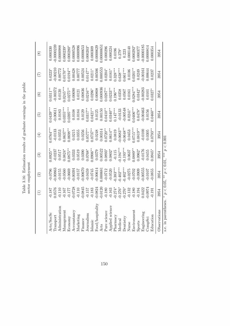
Tab
le3.1
6:
Est
imati
on
resu
lts
of
gra
du
ate
earn
ings
inth
ep
ub
lic
sect
or
emplo
ym
ent
(1)
(2)
(3)
(4)
(5)
(6)
(7)
(8)
Art
s/S
ocS
c-0
.187
-0.0
796
0.0
925∗
∗0.0
764∗
∗∗0.0
439∗
∗∗0.0
311∗
∗0.0
223∗
0.0
00330
Tra
nsp
ort
0.0
576
-0.0
0863
-0.0
237
-0.0
133
-0.0
0611
-0.0
0372
-0.0
0210
-0.0
000239
Ad
min
istr
atio
n-0
.110
-0.0
155
0.0
517
0.0
353
0.0
183
0.0
120
0.0
0772
0.0
000988
Man
agem
ent
-0.1
67
-0.0
560
0.0
824∗
0.0
637∗
∗0.0
355∗
∗∗0.0
245∗
∗∗0.0
170∗
∗0.0
00239∗
Eco
nom
y-0
.177
-0.0
669
0.0
875∗∗
0.0
698∗
∗0.0
395∗
∗∗0.0
275∗
∗0.0
194∗
∗0.0
00280∗
Acc
ounta
ncy
-0.0
728
-0.0
0391
0.0
333
0.0
215
0.0
108
0.0
0690
0.0
0428
0.0
000528
Mar
keti
ng
-0.1
10
-0.0
157
0.0
519
0.0
355
0.0
184
0.0
121
0.0
0777
0.0
000996
Fin
ance
-0.0
845
-0.0
0670
0.0
390
0.0
256
0.0
129
0.0
0836
0.0
0524
0.0
000653
Jou
rnal
ism
-0.1
57
-0.0
459
0.0
768∗
0.0
577∗
∗0.0
317∗
∗0.0
216∗
∗0.0
147∗
∗0.0
00203∗
Isla
mic
-0.1
83
-0.0
745
0.0
906∗∗
0.0
737∗
∗0.0
421∗
∗0.0
296∗
0.0
211∗
0.0
00309
Food
/hos
pit
alit
y-0
.0824
-0.0
0614
0.0
379
0.0
248
0.0
125
0.0
0808
0.0
0506
0.0
000629
Art
s-0
.0120
0.0
00681
0.0
0522
0.0
0314
0.0
0150
0.0
00936
0.0
00553
0.0
0000651
Pu
resc
ien
ce-0
.180
-0.0
712
0.0
893∗
0.0
720∗
∗0.0
410∗
∗0.0
287∗
∗0.0
204∗
0.0
00296
Ap
pli
edsc
ien
ce-0
.163
-0.0
520
0.0
802∗
0.0
614∗
∗0.0
340∗
∗0.0
233∗
∗0.0
161∗
0.0
00224
Ph
arm
acy
-0.2
74∗
-0.3
83∗
∗∗-0
.115
0.0
819
0.1
47∗
∗∗0.1
96∗∗
∗0.3
28∗∗
∗0.0
196
Med
ical
-0.2
76∗
-0.4
02∗
∗∗-0
.194∗∗
∗-0
.0683∗∗
-0.0
133
0.0
358
0.6
38∗∗
∗0.2
79∗
Den
tist
ry-0
.276∗
-0.4
02∗
∗∗-0
.193∗∗
∗-0
.0648∗∗
-0.0
0548
0.0
567
0.6
61∗
∗∗0.2
23
Nu
rse
-0.1
32
-0.0
275
0.0
637
0.0
453
0.0
241∗
0.0
161
0.0
106
0.0
00140
Envir
onm
ent
-0.1
80
-0.0
702
0.0
889∗
∗0.0
715∗
∗∗0.0
406∗
∗∗0.0
284∗
∗∗0.0
201∗
∗0.0
00292∗
Sp
orts
-0.1
94
-0.0
909
0.0
962∗
0.0
819∗
∗0.0
478∗
0.0
342∗
0.0
249
0.0
00377
En
gin
eeri
ng
0.0
422
-0.0
0555
-0.0
176
-0.0
100
-0.0
0463
-0.0
0283
-0.0
0161
-0.0
000185
Com
pS
ci-0
.0974
-0.0
107
0.0
455
0.0
305
0.0
156
0.0
101
0.0
0644
0.0
000814
Ed
uca
tion
-0.1
91
-0.0
855
0.0
945∗
0.0
793∗
∗0.0
460∗
∗0.0
327∗
0.0
237
0.0
00354
Ob
serv
atio
ns
3954
3954
3954
3954
3954
3954
3954
3954
s.e.
inp
aren
thes
es.
∗p<
0.0
5,∗∗p<
0.01,∗∗
∗p<
0.001
150
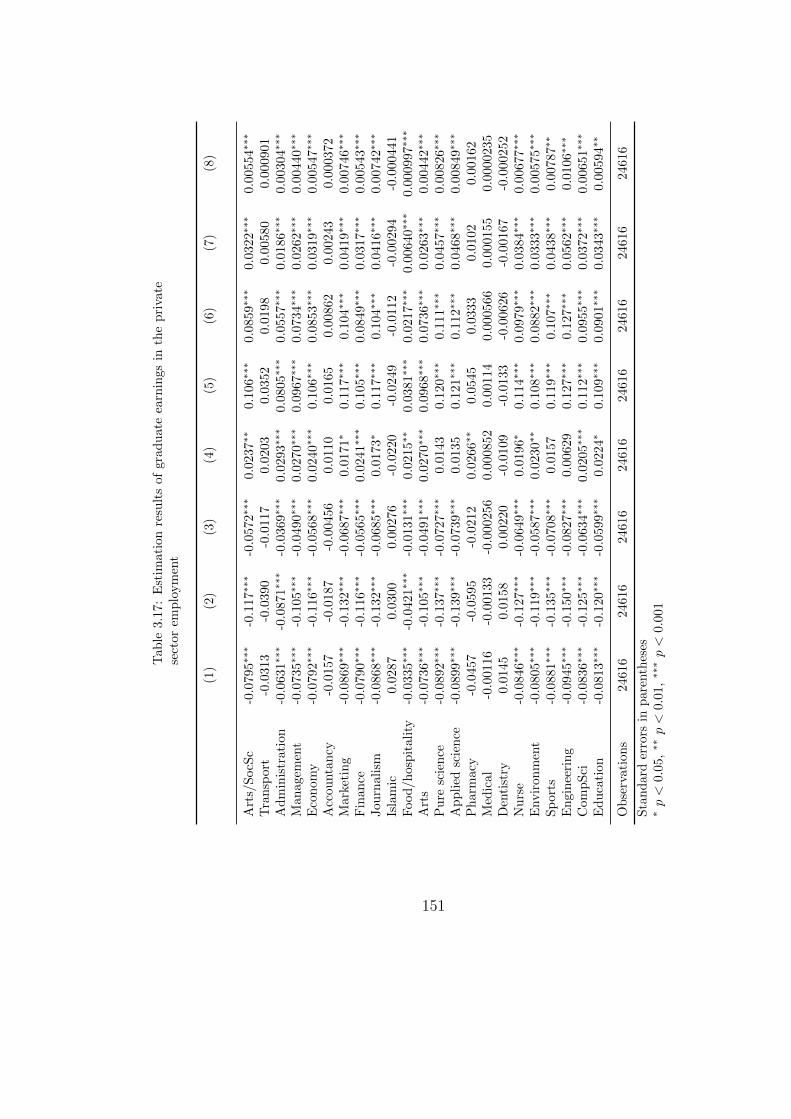
Tab
le3.1
7:
Est
imati
on
resu
lts
of
gra
du
ate
earn
ings
inth
ep
riva
tese
ctor
emplo
ym
ent
(1)
(2)
(3)
(4)
(5)
(6)
(7)
(8)
Art
s/S
ocS
c-0
.0795∗∗
∗-0
.117∗∗
∗-0
.0572∗∗
∗0.0
237∗
∗0.1
06∗∗
∗0.0
859∗
∗∗0.0
322∗∗
∗0.0
0554∗
∗∗
Tra
nsp
ort
-0.0
313
-0.0
390
-0.0
117
0.0
203
0.0
352
0.0
198
0.0
0580
0.0
00901
Ad
min
istr
atio
n-0
.0631∗
∗∗-0
.0871∗∗
∗-0
.0369∗∗
∗0.0
293∗
∗∗0.0
805∗
∗∗0.0
557∗
∗∗0.0
186∗
∗∗0.0
0304∗
∗∗
Man
agem
ent
-0.0
735∗∗
∗-0
.105∗
∗∗-0
.0490∗∗
∗0.0
270∗
∗∗0.0
967∗
∗∗0.0
734∗∗
∗0.0
262∗
∗∗0.0
0440∗
∗∗
Eco
nom
y-0
.0792∗
∗∗-0
.116∗
∗∗-0
.0568∗∗
∗0.0
240∗
∗∗0.1
06∗∗
∗0.0
853∗
∗∗0.0
319∗
∗∗0.0
0547∗
∗∗
Acc
ounta
ncy
-0.0
157
-0.0
187
-0.0
0456
0.0
110
0.0
165
0.0
0862
0.0
0243
0.0
00372
Mar
keti
ng
-0.0
869∗∗
∗-0
.132∗
∗∗-0
.0687∗∗
∗0.0
171∗
0.1
17∗∗
∗0.1
04∗∗
∗0.0
419∗
∗∗0.0
0746∗
∗∗
Fin
ance
-0.0
790∗
∗∗-0
.116∗
∗∗-0
.0565∗∗
∗0.0
241∗
∗∗0.1
05∗∗
∗0.0
849∗
∗∗0.0
317∗
∗∗0.0
0543∗
∗∗
Jou
rnal
ism
-0.0
868∗∗
∗-0
.132∗
∗∗-0
.0685∗∗
∗0.0
173∗
0.1
17∗∗
∗0.1
04∗∗
∗0.0
416∗
∗∗0.0
0742∗
∗∗
Isla
mic
0.0287
0.0
300
0.0
0276
-0.0
220
-0.0
249
-0.0
112
-0.0
0294
-0.0
00441
Food
/hos
pit
alit
y-0
.0335∗∗
∗-0
.0421∗∗
∗-0
.0131∗∗
∗0.0
215∗
∗0.0
381∗
∗∗0.0
217∗
∗∗0.0
0640∗∗
∗0.0
00997∗∗
∗
Art
s-0
.0736∗∗
∗-0
.105∗
∗∗-0
.0491∗∗
∗0.0
270∗
∗∗0.0
968∗
∗∗0.0
736∗
∗∗0.0
263∗
∗∗0.0
0442∗
∗∗
Pu
resc
ien
ce-0
.0892∗
∗∗-0
.137∗
∗∗-0
.0727∗∗
∗0.0
143
0.1
20∗
∗∗0.1
11∗∗
∗0.0
457∗
∗∗0.0
0826∗
∗∗
Ap
pli
edsc
ien
ce-0
.0899∗∗
∗-0
.139∗
∗∗-0
.0739∗∗
∗0.0
135
0.1
21∗
∗∗0.1
12∗∗
∗0.0
468∗
∗∗0.0
0849∗
∗∗
Ph
arm
acy
-0.0
457
-0.0
595
-0.0
212
0.0
266∗∗
0.0
545
0.0
333
0.0
102
0.0
0162
Med
ical
-0.0
0116
-0.0
0133
-0.0
00256
0.0
00852
0.0
0114
0.0
00566
0.0
00155
0.0
000235
Den
tist
ry0.
0145
0.0
158
0.0
0220
-0.0
109
-0.0
133
-0.0
0626
-0.0
0167
-0.0
00252
Nu
rse
-0.0
846∗∗
∗-0
.127∗
∗∗-0
.0649∗∗
∗0.0
196∗
0.1
14∗∗
∗0.0
979∗
∗∗0.0
384∗
∗∗0.0
0677∗
∗∗
Envir
onm
ent
-0.0
805∗∗
∗-0
.119∗
∗∗-0
.0587∗∗
∗0.0
230∗
∗0.1
08∗∗
∗0.0
882∗
∗∗0.0
333∗
∗∗0.0
0575∗
∗∗
Sp
orts
-0.0
881∗∗
∗-0
.135∗
∗∗-0
.0708∗∗
∗0.0
157
0.1
19∗
∗∗0.1
07∗∗
∗0.0
438∗
∗∗0.0
0787∗
∗
En
gin
eeri
ng
-0.0
945∗
∗∗-0
.150∗
∗∗-0
.0827∗∗
∗0.0
0629
0.1
27∗
∗∗0.1
27∗∗
∗0.0
562∗
∗∗0.0
106∗
∗∗
Com
pS
ci-0
.0836∗∗
∗-0
.125∗
∗∗-0
.0634∗∗
∗0.0
205∗
∗∗0.1
12∗∗
∗0.0
955∗
∗∗0.0
372∗
∗∗0.0
0651∗
∗∗
Ed
uca
tion
-0.0
813∗
∗∗-0
.120∗
∗∗-0
.0599∗∗
∗0.0
224∗
0.1
09∗∗
∗0.0
901∗
∗∗0.0
343∗
∗∗0.0
0594∗
∗
Ob
serv
atio
ns
24616
24616
24616
24616
24616
24616
24616
24616
Sta
nd
ard
erro
rsin
par
enth
eses
∗p<
0.05
,∗∗p<
0.0
1,∗∗
∗p<
0.001
151
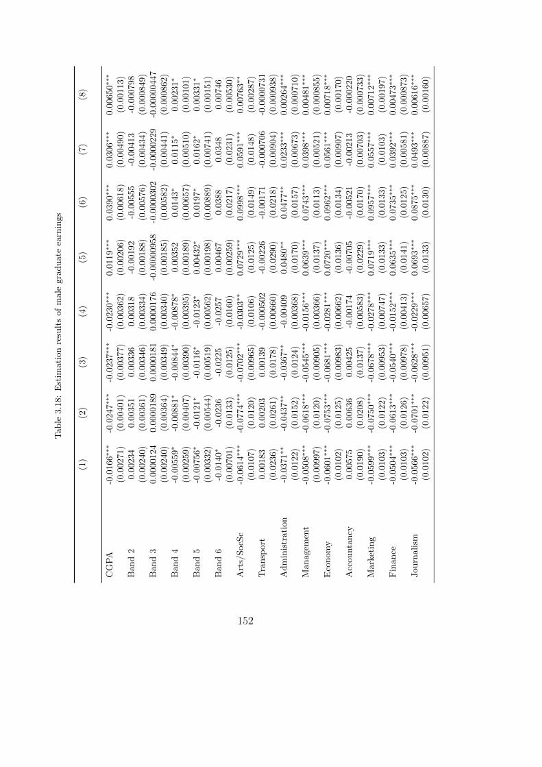
Tab
le3.1
8:
Est
imati
on
resu
lts
of
male
gra
du
ate
earn
ings
(1)
(2)
(3)
(4)
(5)
(6)
(7)
(8)
CG
PA
-0.0
166∗∗
∗-0
.0247∗∗
∗-0
.0237∗∗
∗-0
.0230∗∗
∗0.0
119∗
∗∗0.0
390∗
∗∗0.0
306∗
∗∗0.0
0650∗
∗∗
(0.0
0271)
(0.0
0401)
(0.0
0377)
(0.0
0362)
(0.0
0206)
(0.0
0618)
(0.0
0490)
(0.0
0113)
Ban
d2
0.00
234
0.0
0351
0.0
0336
0.0
0318
-0.0
0192
-0.0
0555
-0.0
0413
-0.0
00798
(0.0
0240)
(0.0
0361)
(0.0
0346)
(0.0
0334)
(0.0
0188)
(0.0
0576)
(0.0
0434)
(0.0
00849)
Ban
d3
0.00
00124
0.0
000189
0.0
000181
0.0
000176
-0.0
0000958
-0.0
000302
-0.0
000229
-0.0
0000447
(0.0
0240)
(0.0
0364)
(0.0
0349)
(0.0
0340)
(0.0
0185)
(0.0
0582)
(0.0
0441)
(0.0
00862)
Ban
d4
-0.0
0559∗
-0.0
0881∗
-0.0
0844∗
-0.0
0878∗
0.0
0352
0.0
143∗
0.0
115∗
0.0
0231∗
(0.0
0259)
(0.0
0407)
(0.0
0390)
(0.0
0395)
(0.0
0189)
(0.0
0657)
(0.0
0510)
(0.0
0101)
Ban
d5
-0.0
0756∗
-0.0
121∗
-0.0
116∗
-0.0
123∗
0.0
0432∗
0.0
197∗
0.0
162∗
0.0
0331∗
(0.0
0332)
(0.0
0544)
(0.0
0519)
(0.0
0562)
(0.0
0198)
(0.0
0889)
(0.0
0741)
(0.0
0151)
Ban
d6
-0.0
140∗
-0.0
236
-0.0
225
-0.0
257
0.0
0467
0.0
388
0.0
348
0.0
0746
(0.0
0701)
(0.0
133)
(0.0
125)
(0.0
160)
(0.0
0259)
(0.0
217)
(0.0
231)
(0.0
0530)
Art
s/S
ocS
c-0
.0614∗
∗∗-0
.0774∗∗
∗-0
.0702∗∗
∗-0
.0303∗∗
0.0
729∗
∗∗0.0
998∗
∗∗0.0
591∗
∗∗0.0
0763∗∗
(0.0
107)
(0.0
120)
(0.0
0965)
(0.0
106)
(0.0
125)
(0.0
149)
(0.0
148)
(0.0
0287)
Tra
nsp
ort
0.00
183
0.0
0203
0.0
0139
-0.0
00502
-0.0
0226
-0.0
0171
-0.0
00706
-0.0
000731
(0.0
236)
(0.0
261)
(0.0
178)
(0.0
0660)
(0.0
290)
(0.0
218)
(0.0
0904)
(0.0
00938)
Ad
min
istr
atio
n-0
.0371∗∗
-0.0
437∗∗
-0.0
367∗∗
-0.0
0409
0.0
480∗
∗0.0
477∗
∗0.0
233∗
∗∗0.0
0264∗∗
∗
(0.0
122)
(0.0
152)
(0.0
124)
(0.0
0368)
(0.0
170)
(0.0
157)
(0.0
0673)
(0.0
00710)
Man
agem
ent
-0.0
508∗
∗∗-0
.0618∗∗
∗-0
.0545∗∗
∗-0
.0156∗∗
∗0.0
639∗
∗∗0.0
743∗
∗∗0.0
398∗
∗∗0.0
0481∗∗
∗
(0.0
0997)
(0.0
120)
(0.0
0905)
(0.0
0366)
(0.0
137)
(0.0
113)
(0.0
0521)
(0.0
00855)
Eco
nom
y-0
.0601∗
∗∗-0
.0753∗∗
∗-0
.0681∗∗
∗-0
.0281∗∗
∗0.0
720∗
∗∗0.0
962∗
∗∗0.0
561∗
∗∗0.0
0718∗∗
∗
(0.0
102)
(0.0
125)
(0.0
0983)
(0.0
0662)
(0.0
136)
(0.0
134)
(0.0
0907)
(0.0
0170)
Acc
ounta
ncy
0.00
575
0.0
0636
0.0
0425
-0.0
0174
-0.0
0705
-0.0
0521
-0.0
0213
-0.0
00220
(0.0
190)
(0.0
208)
(0.0
137)
(0.0
0583)
(0.0
229)
(0.0
170)
(0.0
0703)
(0.0
00733)
Mar
keti
ng
-0.0
599∗
∗∗-0
.0750∗∗
∗-0
.0678∗∗
∗-0
.0278∗∗
∗0.0
719∗
∗∗0.0
957∗
∗∗0.0
557∗
∗∗0.0
0712∗∗
∗
(0.0
103)
(0.0
122)
(0.0
0953)
(0.0
0747)
(0.0
133)
(0.0
133)
(0.0
103)
(0.0
0197)
Fin
ance
-0.0
504∗∗
∗-0
.0613∗∗
∗-0
.0540∗∗
∗-0
.0152∗∗
∗0.0
635∗
∗∗0.0
735∗
∗∗0.0
392∗
∗∗0.0
0473∗∗
∗
(0.0
103)
(0.0
126)
(0.0
0978)
(0.0
0413)
(0.0
141)
(0.0
125)
(0.0
0581)
(0.0
00873)
Jou
rnal
ism
-0.0
566∗
∗∗-0
.0701∗∗
∗-0
.0628∗∗
∗-0
.0229∗∗
∗0.0
693∗
∗∗0.0
875∗
∗∗0.0
493∗
∗∗0.0
0616∗∗
∗
(0.0
102)
(0.0
122)
(0.0
0951)
(0.0
0657)
(0.0
133)
(0.0
130)
(0.0
0887)
(0.0
0160)
152
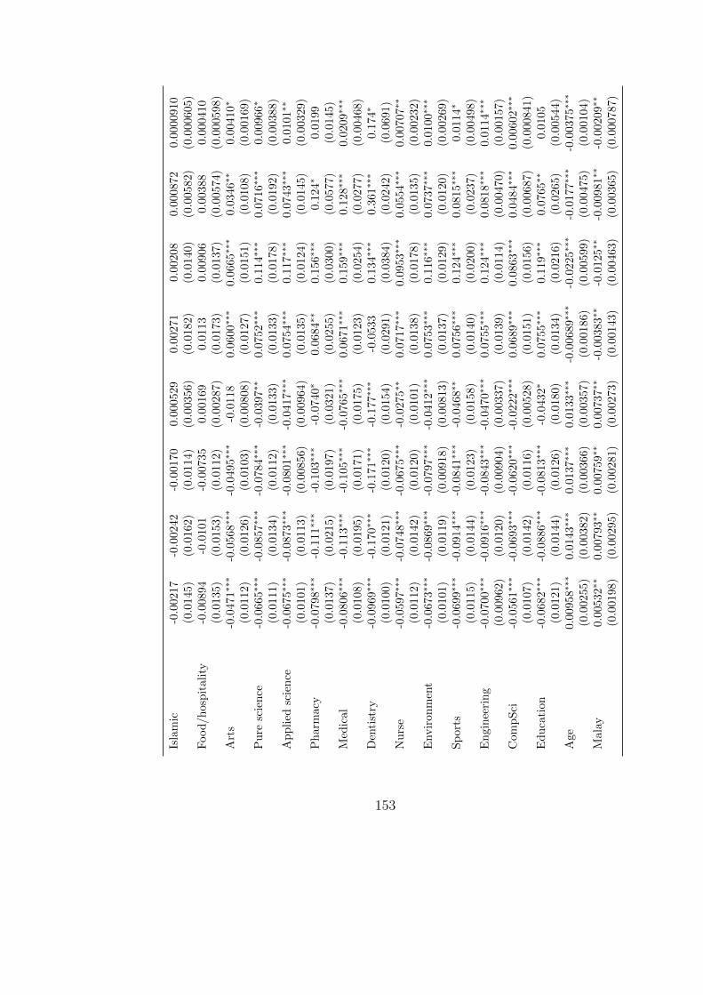
Isla
mic
-0.0
0217
-0.0
0242
-0.0
0170
0.0
00529
0.0
0271
0.0
0208
0.0
00872
0.0
000910
(0.0
145)
(0.0
162)
(0.0
114)
(0.0
0356)
(0.0
182)
(0.0
140)
(0.0
0582)
(0.0
00605)
Food
/hos
pit
alit
y-0
.00894
-0.0
101
-0.0
0735
0.0
0169
0.0
113
0.0
0906
0.0
0388
0.0
00410
(0.0
135)
(0.0
153)
(0.0
112)
(0.0
0287)
(0.0
173)
(0.0
137)
(0.0
0574)
(0.0
00598)
Art
s-0
.0471∗
∗∗-0
.0568∗∗
∗-0
.0495∗∗
∗-0
.0118
0.0
600∗
∗∗0.0
665∗∗
∗0.0
346∗
∗0.0
0410∗
(0.0
112)
(0.0
126)
(0.0
103)
(0.0
0808)
(0.0
127)
(0.0
151)
(0.0
108)
(0.0
0169)
Pu
resc
ien
ce-0
.0665∗
∗∗-0
.0857∗∗
∗-0
.0784∗∗
∗-0
.0397∗∗
0.0
752∗
∗∗0.1
14∗∗
∗0.0
716∗
∗∗0.0
0966∗
(0.0
111)
(0.0
134)
(0.0
112)
(0.0
133)
(0.0
133)
(0.0
178)
(0.0
192)
(0.0
0388)
Ap
pli
edsc
ien
ce-0
.0675∗∗
∗-0
.0873∗∗
∗-0
.0801∗∗
∗-0
.0417∗∗
∗0.0
754∗
∗∗0.1
17∗∗
∗0.0
743∗
∗∗0.0
101∗
∗
(0.0
101)
(0.0
113)
(0.0
0856)
(0.0
0964)
(0.0
135)
(0.0
124)
(0.0
145)
(0.0
0329)
Ph
arm
acy
-0.0
798∗∗
∗-0
.111∗∗
∗-0
.103∗∗
∗-0
.0740∗
0.0
684∗
∗0.1
56∗∗
∗0.1
24∗
0.0
199
(0.0
137)
(0.0
215)
(0.0
197)
(0.0
321)
(0.0
255)
(0.0
300)
(0.0
577)
(0.0
145)
Med
ical
-0.0
806∗
∗∗-0
.113∗∗
∗-0
.105∗∗
∗-0
.0765∗∗
∗0.0
671∗
∗∗0.1
59∗∗
∗0.1
28∗∗
∗0.0
209∗
∗∗
(0.0
108)
(0.0
195)
(0.0
171)
(0.0
175)
(0.0
123)
(0.0
254)
(0.0
277)
(0.0
0468)
Den
tist
ry-0
.0969∗∗
∗-0
.170∗∗
∗-0
.171∗∗
∗-0
.177∗∗
∗-0
.0533
0.1
34∗∗
∗0.3
61∗∗
∗0.1
74∗
(0.0
100)
(0.0
121)
(0.0
120)
(0.0
154)
(0.0
291)
(0.0
384)
(0.0
242)
(0.0
691)
Nu
rse
-0.0
597∗∗
∗-0
.0748∗∗
∗-0
.0675∗∗
∗-0
.0275∗∗
0.0
717∗
∗∗0.0
953∗∗
∗0.0
554∗
∗∗0.0
0707∗
∗
(0.0
112)
(0.0
142)
(0.0
120)
(0.0
101)
(0.0
138)
(0.0
178)
(0.0
135)
(0.0
0232)
Envir
onm
ent
-0.0
673∗∗
∗-0
.0869∗∗
∗-0
.0797∗∗
∗-0
.0412∗∗
∗0.0
753∗
∗∗0.1
16∗∗
∗0.0
737∗
∗∗0.0
100∗
∗∗
(0.0
101)
(0.0
119)
(0.0
0918)
(0.0
0813)
(0.0
137)
(0.0
129)
(0.0
120)
(0.0
0269)
Sp
orts
-0.0
699∗∗
∗-0
.0914∗∗
∗-0
.0841∗∗
∗-0
.0468∗∗
0.0
756∗
∗∗0.1
24∗∗
∗0.0
815∗
∗∗0.0
114∗
(0.0
115)
(0.0
144)
(0.0
123)
(0.0
158)
(0.0
140)
(0.0
200)
(0.0
237)
(0.0
0498)
En
gin
eeri
ng
-0.0
700∗∗
∗-0
.0916∗∗
∗-0
.0843∗∗
∗-0
.0470∗∗
∗0.0
755∗
∗∗0.1
24∗∗
∗0.0
818∗
∗∗0.0
114∗
∗∗
(0.0
0962)
(0.0
120)
(0.0
0904)
(0.0
0337)
(0.0
139)
(0.0
114)
(0.0
0470)
(0.0
0157)
Com
pS
ci-0
.0561∗
∗∗-0
.0693∗∗
∗-0
.0620∗∗
∗-0
.0222∗∗
∗0.0
689∗
∗∗0.0
863∗
∗∗0.0
484∗∗
∗0.0
0602∗
∗∗
(0.0
107)
(0.0
142)
(0.0
116)
(0.0
0528)
(0.0
151)
(0.0
156)
(0.0
0687)
(0.0
00841)
Ed
uca
tion
-0.0
682∗∗
∗-0
.0886∗∗
∗-0
.0813∗∗
∗-0
.0432∗
0.0
755∗∗
∗0.1
19∗∗
∗0.0
765∗
∗0.0
105
(0.0
121)
(0.0
144)
(0.0
126)
(0.0
180)
(0.0
134)
(0.0
216)
(0.0
265)
(0.0
0544)
Age
0.00
958∗
∗∗0.0
143∗
∗∗0.0
137∗
∗∗0.0
133∗
∗∗-0
.00689∗∗
∗-0
.0225∗∗
∗-0
.0177∗∗
∗-0
.00375∗
∗∗
(0.0
0255)
(0.0
0382)
(0.0
0366)
(0.0
0357)
(0.0
0186)
(0.0
0599)
(0.0
0475)
(0.0
0104)
Mal
ay0.
00532∗
∗0.0
0793∗
∗0.0
0759∗
∗0.0
0737∗
∗-0
.00383∗∗
-0.0
125∗∗
-0.0
0981∗∗
-0.0
0209∗
∗
(0.0
0198)
(0.0
0295)
(0.0
0281)
(0.0
0273)
(0.0
0143)
(0.0
0463)
(0.0
0365)
(0.0
00787)
153
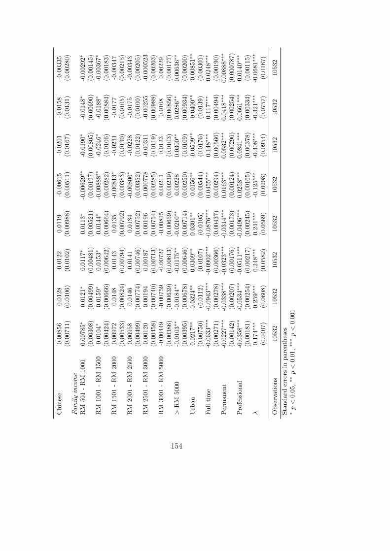
Ch
ines
e0.
00856
0.0
128
0.0
122
0.0
119
-0.0
0615
-0.0
201
-0.0
158
-0.0
0335
(0.0
0711)
(0.0
106)
(0.0
102)
(0.0
0988)
(0.0
0511)
(0.0
167)
(0.0
131)
(0.0
0280)
Familyincome
RM
501
-R
M10
000.
00785∗
0.0
121∗
0.0
117∗
0.0
113∗
-0.0
0629∗
∗-0
.0190∗
-0.0
148∗
-0.0
0292∗
(0.0
0308)
(0.0
0499)
(0.0
0481)
(0.0
0521)
(0.0
0197)
(0.0
0805)
(0.0
0690)
(0.0
0145)
RM
1001
-R
M15
000.
0104∗
0.0
159∗
0.0
153∗
0.0
144∗
-0.0
0888∗
∗-0
.0246∗
-0.0
188∗
-0.0
0367∗
(0.0
0424)
(0.0
0666)
(0.0
0642)
(0.0
0664)
(0.0
0282)
(0.0
106)
(0.0
0884)
(0.0
0183)
RM
1501
-R
M20
000.
00972
0.0
148
0.0
143
0.0
135
-0.0
0813∗
-0.0
231
-0.0
177
-0.0
0347
(0.0
0533)
(0.0
0824)
(0.0
0794)
(0.0
0792)
(0.0
0383)
(0.0
130)
(0.0
105)
(0.0
0215)
RM
2001
-R
M25
000.
00958
0.0
146
0.0
141
0.0
134
-0.0
0800∗
-0.0
228
-0.0
175
-0.0
0343
(0.0
0499)
(0.0
0774)
(0.0
0746)
(0.0
0752)
(0.0
0352)
(0.0
122)
(0.0
100)
(0.0
0205)
RM
2501
-R
M30
000.
00120
0.0
0194
0.0
0187
0.0
0196
-0.0
00778
-0.0
0311
-0.0
0255
-0.0
00523
(0.0
0458)
(0.0
0740)
(0.0
0713)
(0.0
0754)
(0.0
0285)
(0.0
119)
(0.0
0988)
(0.0
0203)
RM
3001
-R
M50
00-0
.00449
-0.0
0759
-0.0
0727
-0.0
0815
0.0
0211
0.0
123
0.0
108
0.0
0229
(0.0
0386)
(0.0
0639)
(0.0
0613)
(0.0
0659)
(0.0
0239)
(0.0
103)
(0.0
0856)
(0.0
0177)
>R
M50
00-0
.0103∗
∗-0
.0184∗∗
-0.0
175∗∗
-0.0
210∗∗
0.0
0228
0.0
300∗
∗0.0
286∗
∗0.0
0636∗
∗
(0.0
0395)
(0.0
0678)
(0.0
0646)
(0.0
0714)
(0.0
0250)
(0.0
109)
(0.0
0934)
(0.0
0200)
Urb
an0.
0217∗∗
0.0
324∗
∗0.0
309∗
∗0.0
301∗
∗-0
.0156∗∗
-0.0
509∗∗
-0.0
400∗∗
-0.0
0851∗
∗
(0.0
0750)
(0.0
112)
(0.0
107)
(0.0
105)
(0.0
0544)
(0.0
176)
(0.0
139)
(0.0
0301)
Fu
llti
me
-0.0
633∗∗
∗-0
.0943∗∗
∗-0
.0902∗∗
∗-0
.0876∗∗
∗0.0
455∗
∗∗0.1
48∗∗
∗0.1
17∗
∗∗0.0
248∗
∗∗
(0.0
0271)
(0.0
0278)
(0.0
0366)
(0.0
0437)
(0.0
0294)
(0.0
0566)
(0.0
0494)
(0.0
0190)
Per
man
ent
-0.0
227∗∗
∗-0
.0338∗∗
∗-0
.0323∗∗
∗-0
.0314∗∗
∗0.0
163∗
∗∗0.0
532∗
∗∗0.0
418∗
∗∗0.0
0888∗∗
∗
(0.0
0142)
(0.0
0207)
(0.0
0176)
(0.0
0173)
(0.0
0124)
(0.0
0290)
(0.0
0254)
(0.0
00787)
Pro
fess
ion
al-0
.0358∗∗
∗-0
.0534∗∗
∗-0
.0511∗∗
∗-0
.0496∗∗
∗0.0
258∗
∗∗0.0
841∗
∗∗0.0
661∗
∗∗0.0
140∗
∗∗
(0.0
0181)
(0.0
0254)
(0.0
0217)
(0.0
0245)
(0.0
0165)
(0.0
0378)
(0.0
0334)
(0.0
0115)
λ0.
174∗
∗∗0.2
59∗∗
∗0.2
48∗∗
∗0.2
41∗∗
∗-0
.125∗∗
∗-0
.408∗∗
∗-0
.321∗∗
∗-0
.0681∗∗
∗
(0.0
407)
(0.0
608)
(0.0
582)
(0.0
569)
(0.0
298)
(0.0
954)
(0.0
757)
(0.0
167)
Ob
serv
atio
ns
10532
10532
10532
10532
10532
10532
10532
10532
Sta
nd
ard
erro
rsin
par
enth
eses
∗p<
0.05
,∗∗p<
0.01
,∗∗
∗p<
0.0
01
154

Tab
le3.1
9:
Est
imati
on
resu
lts
of
fem
ale
gra
du
ate
earn
ings
(1)
(2)
(3)
(4)
(5)
(6)
(7)
(8)
CG
PA
-0.0
137∗
∗∗-0
.0268∗∗
∗-0
.0113∗
∗∗0.0
0378∗
∗∗0.0
189∗
∗∗0.0
161∗
∗∗0.0
116
∗∗∗
0.0
0143∗∗
∗
(0.0
0290)
(0.0
0565)
(0.0
0237)
(0.0
00873)
(0.0
0397)
(0.0
0339)
(0.0
0244)
(0.0
00332)
Ban
d2
-0.0
0167
-0.0
0308
-0.0
0114
0.0
00797
0.0
0229
0.0
0162
0.0
0107
0.0
00104
(0.0
0272)
(0.0
0499)
(0.0
0182)
(0.0
0133)
(0.0
0372)
(0.0
0260)
(0.0
0172)
(0.0
00166)
Ban
d3
-0.0
143∗
∗∗-0
.0286∗∗
∗-0
.0120∗
∗∗0.0
0525∗
∗∗0.0
211∗
∗∗0.0
164∗
∗∗0.0
111
∗∗∗
0.0
0113∗∗
∗
(0.0
0272)
(0.0
0517)
(0.0
0199)
(0.0
0133)
(0.0
0386)
(0.0
0275)
(0.0
0183)
(0.0
00211)
Ban
d4
-0.0
226∗
∗∗-0
.0481∗∗
∗-0
.0218∗
∗∗0.0
0597∗
∗∗0.0
347∗
∗∗0.0
293∗
∗∗0.0
203
∗∗∗
0.0
0218∗∗
∗
(0.0
0291)
(0.0
0591)
(0.0
0257)
(0.0
0134)
(0.0
0437)
(0.0
0343)
(0.0
0236)
(0.0
00317)
Ban
d5
-0.0
267∗
∗∗-0
.0590∗∗
∗-0
.0279∗
∗∗0.0
0531∗
∗∗0.0
419∗
∗∗0.0
372∗
∗∗0.0
262
∗∗∗
0.0
0289∗∗
∗
(0.0
0367)
(0.0
0857)
(0.0
0447)
(0.0
0150)
(0.0
0594)
(0.0
0585)
(0.0
0433)
(0.0
00552)
Ban
d6
0.0455
0.0
662∗
0.0
148∗
∗∗-0
.0300
-0.0
485∗
-0.0
283∗∗
-0.0
181∗∗
-0.0
0153∗
∗
(0.0
260)
(0.0
305)
(0.0
0266)
(0.0
191)
(0.0
215)
(0.0
109)
(0.0
0677)
(0.0
00528)
Art
s/S
ocS
c-0
.0978∗∗
∗-0
.127∗∗
∗-0
.0241∗∗
∗0.0
579∗
∗∗0.0
951∗
∗∗0.0
632∗
∗∗0.0
307∗
∗∗0.0
0158∗
∗
(0.0
126)
(0.0
119)
(0.0
0549)
(0.0
0878)
(0.0
0855)
(0.0
0901)
(0.0
0730)
(0.0
00507)
Tra
nsp
ort
-0.0
582∗∗
-0.0
615∗
-0.0
0227
0.0
393∗
0.0
468∗
0.0
251∗
0.0
102∗
0.0
00485∗
(0.0
225)
(0.0
285)
(0.0
0476)
(0.0
161)
(0.0
215)
(0.0
119)
(0.0
0494)
(0.0
00241)
Ad
min
istr
atio
n-0
.0879∗
∗∗-0
.108∗∗
∗-0
.0160∗∗
∗0.0
549∗
∗∗0.0
814∗
∗∗0.0
506∗∗
∗0.0
232
∗∗∗
0.0
0116∗
∗∗
(0.0
135)
(0.0
178)
(0.0
0426)
(0.0
103)
(0.0
135)
(0.0
0692)
(0.0
0258)
(0.0
00178)
Man
agem
ent
-0.0
962∗∗
∗-0
.123∗∗
∗-0
.0226∗∗
∗0.0
575∗∗
∗0.0
927∗
∗∗0.0
609∗∗
∗0.0
293∗∗
∗0.0
0150∗
∗∗
(0.0
119)
(0.0
125)
(0.0
0236)
(0.0
0937)
(0.0
0966)
(0.0
0414)
(0.0
0241)
(0.0
00241)
Eco
nom
y-0
.101∗
∗∗-0
.134∗∗
∗-0
.0274∗∗
∗0.0
584∗∗
∗0.1
00∗
∗∗0.0
682∗∗
∗0.0
339∗∗
∗0.0
0177∗
∗∗
(0.0
121)
(0.0
129)
(0.0
0364)
(0.0
0930)
(0.0
0986)
(0.0
0590)
(0.0
0436)
(0.0
00361)
Acc
ounta
ncy
-0.0
405∗
-0.0
396
0.0
00995
0.0
278
0.0
300
0.0
151
0.0
0588∗
0.0
00274∗
(0.0
198)
(0.0
216)
(0.0
0189)
(0.0
147)
(0.0
161)
(0.0
0771)
(0.0
0285)
(0.0
00133)
Mar
keti
ng
-0.1
11∗∗
∗-0
.157∗∗
∗-0
.0395∗∗
∗0.0
580∗∗
∗0.1
15∗
∗∗0.0
856∗
∗∗0.0
462
∗∗∗
0.0
0254∗
∗∗
(0.0
120)
(0.0
124)
(0.0
0455)
(0.0
0958)
(0.0
0941)
(0.0
0711)
(0.0
0690)
(0.0
00600)
Fin
ance
-0.1
04∗
∗∗-0
.140∗∗
∗-0
.0304∗∗
∗0.0
586∗∗
∗0.1
04∗
∗∗0.0
726∗
∗∗0.0
368∗
∗∗0.0
0195∗
∗∗
(0.0
120)
(0.0
138)
(0.0
0339)
(0.0
0936)
(0.0
107)
(0.0
0516)
(0.0
0295)
(0.0
00309)
Jou
rnal
ism
-0.1
12∗∗
∗-0
.158∗∗
∗-0
.0403∗∗
∗0.0
579∗∗
∗0.1
16∗
∗∗0.0
866∗
∗∗0.0
470∗
∗∗0.0
0259∗
∗∗
(0.0
119)
(0.0
123)
(0.0
0388)
(0.0
0951)
(0.0
0956)
(0.0
0599)
(0.0
0578)
(0.0
00543)
155

Isla
mic
0.00761
0.0
0609
-0.0
0115
-0.0
0516
-0.0
0460
-0.0
0203
-0.0
00730
-0.0
000330
(0.0
169)
(0.0
135)
(0.0
0252)
(0.0
114)
(0.0
102)
(0.0
0458)
(0.0
0167)
(0.0
000759)
Food
/hos
pit
alit
y-0
.0566∗∗
∗-0
.0595∗∗
∗-0
.00187
0.0
384∗∗
∗0.0
452∗
∗∗0.0
241∗
∗∗0.0
0980∗∗
∗0.0
004
64∗
∗∗
(0.0
142)
(0.0
152)
(0.0
0218)
(0.0
106)
(0.0
113)
(0.0
0537)
(0.0
0206)
(0.0
00110)
Art
s-0
.0943∗∗
∗-0
.120∗∗
∗-0
.0210∗∗
∗0.0
571∗
∗∗0.0
902∗
∗∗0.0
585∗
∗∗0.0
278∗
∗∗0.0
0142∗∗
(0.0
128)
(0.0
127)
(0.0
0538)
(0.0
0867)
(0.0
0924)
(0.0
0892)
(0.0
0671)
(0.0
00452)
Pu
resc
ien
ce-0
.104∗
∗∗-0
.139∗∗
∗-0
.0301∗∗
∗0.0
586∗
∗∗0.1
04∗∗
∗0.0
721∗
∗∗0.0
365∗
∗∗0.0
0193∗∗
(0.0
128)
(0.0
134)
(0.0
0675)
(0.0
0922)
(0.0
0933)
(0.0
106)
(0.0
0903)
(0.0
00648)
Ap
pli
edsc
ien
ce-0
.108∗∗
∗-0
.149∗∗
∗-0
.0353∗∗
∗0.0
585∗
∗∗0.1
10∗∗
∗0.0
796∗
∗∗0.0
417∗
∗∗0.0
0225∗∗
∗
(0.0
121)
(0.0
108)
(0.0
0517)
(0.0
0958)
(0.0
0778)
(0.0
0830)
(0.0
0833)
(0.0
00657)
Ph
arm
acy
-0.1
21∗
∗∗-0
.185∗∗
∗-0
.0568∗∗
0.0
527∗
∗∗0.1
31∗∗
∗0.1
09∗
∗∗0.0
662∗
0.0
0393
(0.0
152)
(0.0
273)
(0.0
196)
(0.0
155)
(0.0
129)
(0.0
268)
(0.0
292)
(0.0
0237)
Med
ical
-0.1
38∗
∗∗-0
.249∗∗
∗-0
.107∗∗
∗0.0
171
0.1
47∗∗
∗0.1
70∗
∗∗0.1
48∗
∗∗0.0
120∗
∗∗
(0.0
120)
(0.0
236)
(0.0
161)
(0.0
117)
(0.0
105)
(0.0
182)
(0.0
220)
(0.0
0229)
Den
tist
ry-0
.146∗
∗∗-0
.307∗∗
∗-0
.180∗∗
∗-0
.0718∗∗
0.0
917∗
∗∗0.1
99∗∗
∗0.3
49∗∗
∗0.0
650∗
(0.0
120)
(0.0
121)
(0.0
118)
(0.0
225)
(0.0
259)
(0.0
141)
(0.0
457)
(0.0
272)
Nu
rse
-0.1
04∗∗
∗-0
.140∗∗
∗-0
.0307∗∗
∗0.0
586∗
∗∗0.1
05∗∗
∗0.0
730∗
∗∗0.0
371∗
∗∗0.0
019
7∗∗
∗
(0.0
121)
(0.0
130)
(0.0
0439)
(0.0
0933)
(0.0
0981)
(0.0
0677)
(0.0
0545)
(0.0
00442)
Envir
onm
ent
-0.0
929∗∗
∗-0
.117∗∗
∗-0
.0198∗∗
∗0.0
567∗
∗∗0.0
883∗
∗∗0.0
567∗
∗∗0.0
267∗
∗∗0.0
013
6∗∗
∗
(0.0
122)
(0.0
120)
(0.0
0395)
(0.0
0892)
(0.0
0899)
(0.0
0671)
(0.0
0490)
(0.0
00347)
Sp
orts
-0.1
08∗∗
∗-0
.149∗∗
∗-0
.0354∗∗
0.0
585∗
∗∗0.1
10∗∗
∗0.0
797∗
∗∗0.0
418∗
∗0.0
0226∗
(0.0
151)
(0.0
232)
(0.0
125)
(0.0
0969)
(0.0
152)
(0.0
184)
(0.0
148)
(0.0
0102)
En
gin
eeri
ng
-0.1
15∗
∗∗-0
.166∗∗
∗-0
.0447∗∗
∗0.0
569∗
∗∗0.1
21∗∗
∗0.0
928∗
∗∗0.0
519∗
∗∗0.0
029
1∗∗
∗
(0.0
117)
(0.0
130)
(0.0
0318)
(0.0
0929)
(0.0
104)
(0.0
0460)
(0.0
0341)
(0.0
00462)
Com
pS
ci-0
.107∗∗
∗-0
.146∗∗
∗-0
.0339∗∗
∗0.0
586∗
∗∗0.1
09∗∗
∗0.0
776∗
∗∗0.0
404∗
∗∗0.0
0216∗∗
∗
(0.0
125)
(0.0
173)
(0.0
0540)
(0.0
0926)
(0.0
131)
(0.0
0746)
(0.0
0301)
(0.0
00296)
Ed
uca
tion
-0.0
989∗
∗∗-0
.129∗∗
∗-0
.0251∗∗
0.0
581∗
∗∗0.0
966∗
∗∗0.0
647∗
∗∗0.0
316∗
∗0.0
0164∗
(0.0
147)
(0.0
179)
(0.0
0958)
(0.0
0852)
(0.0
122)
(0.0
151)
(0.0
115)
(0.0
00749)
Age
0.00678∗
0.0
133∗
0.0
0562∗
-0.0
0187∗
-0.0
0935∗
-0.0
0801∗
-0.0
0573∗
-0.0
00707∗
(0.0
0278)
(0.0
0543)
(0.0
0232)
(0.0
00761)
(0.0
0383)
(0.0
0329)
(0.0
0236)
(0.0
00298)
Mal
ay0.
00352
0.0
0689
0.0
0292
-0.0
00974
-0.0
0485
-0.0
0416
-0.0
0298
-0.0
00367
(0.0
0202)
(0.0
0395)
(0.0
0168)
(0.0
00561)
(0.0
0278)
(0.0
0238)
(0.0
0171)
(0.0
00214)
156

Ch
ines
e-0
.00430
-0.0
0842
-0.0
0357
0.0
0119
0.0
0593
0.0
0508
0.0
0364
0.0
00449
(0.0
0776)
(0.0
152)
(0.0
0643)
(0.0
0216)
(0.0
107)
(0.0
0916)
(0.0
0656)
(0.0
00811)
Familyincome
RM
501
-R
M10
000.
00966∗
∗0.0
192∗
∗0.0
0811∗∗
-0.0
0306∗
∗∗-0
.0137∗∗
-0.0
113∗∗
-0.0
0802∗
-0.0
00908∗
(0.0
0316)
(0.0
0668)
(0.0
0315)
(0.0
00707)
(0.0
0466)
(0.0
0429)
(0.0
0316)
(0.0
00388)
RM
1001
-R
M15
000.
00987∗
0.0
196∗
0.0
0826∗
-0.0
0315∗
∗-0
.0140∗
-0.0
115∗
-0.0
0818
-0.0
00924
(0.0
0454)
(0.0
0927)
(0.0
0417)
(0.0
0107)
(0.0
0652)
(0.0
0576)
(0.0
0420)
(0.0
00499)
RM
1501
-R
M20
000.
00813
0.0
163
0.0
0698
-0.0
0246
-0.0
116
-0.0
0967
-0.0
0690
-0.0
00785
(0.0
0575)
(0.0
116)
(0.0
0511)
(0.0
0149)
(0.0
0820)
(0.0
0708)
(0.0
0513)
(0.0
00598)
RM
2001
-R
M25
000.
00190
0.0
0398
0.0
0179
-0.0
00454
-0.0
0280
-0.0
0244
-0.0
0177
-0.0
00206
(0.0
0524)
(0.0
110)
(0.0
0499)
(0.0
0118)
(0.0
0772)
(0.0
0681)
(0.0
0494)
(0.0
00580)
RM
2501
-R
M30
000.
00353
0.0
0731
0.0
0325
-0.0
00908
-0.0
0517
-0.0
0445
-0.0
0320
-0.0
00372
(0.0
0505)
(0.0
105)
(0.0
0475)
(0.0
0116)
(0.0
0739)
(0.0
0650)
(0.0
0472)
(0.0
00554)
RM
3001
-R
M50
00-0
.00387
-0.0
0844
-0.0
0399
0.0
00645
0.0
0585
0.0
0538
0.0
0395
0.0
00474
(0.0
0417)
(0.0
0899)
(0.0
0415)
(0.0
00911)
(0.0
0630)
(0.0
0559)
(0.0
0405)
(0.0
00480)
>R
M50
00-0
.0119∗∗
-0.0
276∗
∗-0
.0140∗∗
0.0
00461
0.0
185∗∗
0.0
186∗
∗0.0
141∗
∗0.0
0176∗∗
(0.0
0425)
(0.0
0955)
(0.0
0456)
(0.0
0100)
(0.0
0665)
(0.0
0603)
(0.0
0441)
(0.0
00553)
Urb
an0.
0126
0.0
247
0.0
105
-0.0
0349
-0.0
174
-0.0
149
-0.0
107
-0.0
0132
(0.0
0819)
(0.0
160)
(0.0
0683)
(0.0
0224)
(0.0
113)
(0.0
0970)
(0.0
0696)
(0.0
00866)
Fu
llti
me
-0.0
731∗
∗∗-0
.143∗∗
∗-0
.0606∗∗
∗0.0
202∗
∗∗0.1
01∗∗
∗0.0
863∗
∗∗0.0
618∗
∗∗0.0
0763∗∗
∗
(0.0
0229)
(0.0
0312)
(0.0
0239)
(0.0
0130)
(0.0
0305)
(0.0
0278)
(0.0
0238)
(0.0
00774)
Per
man
ent
-0.0
354∗
∗∗-0
.0694∗∗
∗-0
.0294∗∗
∗0.0
0980∗∗
∗0.0
489∗
∗∗0.0
419∗
∗∗0.0
300∗
∗∗0.0
0370∗∗
∗
(0.0
0150)
(0.0
0257)
(0.0
0103)
(0.0
00754)
(0.0
0176)
(0.0
0168)
(0.0
0139)
(0.0
00388)
Pro
fess
ion
al-0
.0483∗∗
∗-0
.0945∗∗
∗-0
.0401∗∗
∗0.0
134∗
∗∗0.0
666∗
∗∗0.0
570∗
∗∗0.0
408∗
∗∗0.0
0504∗∗
∗
(0.0
0163)
(0.0
0266)
(0.0
0122)
(0.0
00935)
(0.0
0190)
(0.0
0187)
(0.0
0164)
(0.0
00515)
λ0.
167∗∗
∗0.3
26∗∗
∗0.1
38∗∗
∗-0
.0461∗∗
∗-0
.230∗
∗∗-0
.197∗∗
∗-0
.141∗∗
∗-0
.0174∗∗
∗
(0.0
423)
(0.0
826)
(0.0
355)
(0.0
116)
(0.0
585)
(0.0
502)
(0.0
362)
(0.0
0474)
Ob
serv
atio
ns
18038
18038
18038
18038
18038
18038
1803
818038
Sta
nd
ard
erro
rsin
par
enth
eses
∗p<
0.05
,∗∗p<
0.0
1,∗∗
∗p<
0.001
157
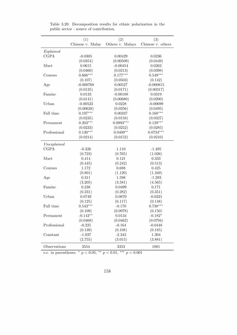
Table 3.20: Decomposition results for ethnic polarization in thepublic sector - source of contribution.
(1) (2) (3)Chinese v. Malay Others v. Malays Chinese v. others
ExplainedCGPA -0.0305 0.00429 0.0236
(0.0354) (0.00509) (0.0449)Muet 0.0615 -0.00454 0.0262
(0.0460) (0.0213) (0.0398)Courses 0.666∗∗∗ 0.177∗∗∗ 0.549∗∗∗
(0.107) (0.0503) (0.142)Age -0.000768 0.00527 -0.000815
(0.0135) (0.0171) (0.00317)Faminc 0.0133 -0.00108 0.0319
(0.0141) (0.00680) (0.0200)Urban -0.00523 0.0228 -0.00699
(0.00638) (0.0356) (0.0495)Full time 0.197∗∗∗ 0.00337 0.168∗∗∗
(0.0235) (0.0158) (0.0327)Permanent 0.203∗∗∗ 0.0993∗∗∗ 0.129∗∗∗
(0.0233) (0.0252) (0.0285)Professional 0.130∗∗∗ 0.0409∗∗ 0.0734∗∗∗
(0.0214) (0.0152) (0.0210)
UnexplainedCGPA -0.326 1.110 -1.495
(0.723) (0.765) (1.026)Muet 0.414 0.121 0.333
(0.445) (0.242) (0.513)Courses 1.172 0.688 0.425
(0.801) (1.120) (1.349)Age 0.311 1.598 -1.293
(3.205) (3.581) (4.565)Faminc 0.238 0.0499 0.171
(0.231) (0.282) (0.351)Urban 0.0749 0.0870 -0.0331
(0.125) (0.117) (0.148)Full time 0.543∗∗∗ -0.170 0.738∗∗∗
(0.109) (0.0978) (0.150)Permanent -0.143∗∗ 0.0134 -0.182∗
(0.0468) (0.0462) (0.0794)Professional -0.225 -0.164 -0.0448
(0.139) (0.108) (0.185)Constant -1.037 -2.342 1.304
(2.755) (3.015) (3.881)
Observations 3554 3353 1001
s.e. in parentheses. ∗ p < 0.05, ∗∗ p < 0.01, ∗∗∗ p < 0.001
158

Table 3.21: Decomposition results for ethnic polarization in theprivate sector - source of contribution.
(1) (2) (3)Chinese v. Malay Others v. Malays Chinese v. others
ExplainedCGPA 0.0237∗∗∗ -0.00975∗∗ 0.0435∗∗∗
(0.00323) (0.00298) (0.00867)Muet 0.0940∗∗∗ 0.0466∗∗∗ 0.0522∗∗∗
(0.0106) (0.00645) (0.00980)Courses -0.0283 0.0203 -0.0230
(0.0145) (0.0140) (0.0234)Age 0.0439∗∗∗ -0.0406∗∗∗ 0.0642∗∗∗
(0.00527) (0.00814) (0.0133)Faminc -0.0372∗∗∗ -0.0173∗∗∗ -0.00698
(0.00590) (0.00463) (0.00907)Urban 0.0103∗ 0.0790∗∗∗ -0.0649∗∗∗
(0.00525) (0.0162) (0.0158)Full time 0.141∗∗∗ 0.0146 0.127∗∗∗
(0.00671) (0.00888) (0.0126)Permanent 0.111∗∗∗ 0.0417∗∗∗ 0.0736∗∗∗
(0.00581) (0.00616) (0.00770)Professional 0.0690∗∗∗ 0.0319∗∗∗ 0.0438∗∗∗
(0.00467) (0.00916) (0.00730)
UnexplainedCGPA 0.501∗∗ 0.306 0.185
(0.164) (0.289) (0.306)Muet -0.0693 -0.0336 -0.0405
(0.151) (0.101) (0.180)Courses 0.914∗∗∗ 0.405 0.483∗
(0.145) (0.223) (0.245)Age 1.306 4.980∗∗ -3.654∗
(1.062) (1.644) (1.795)Faminc 0.0158 0.162 -0.159
(0.0872) (0.117) (0.138)Urban 0.0383 0.152∗ -0.117
(0.0510) (0.0692) (0.0731)Full time 0.581∗∗∗ 0.0771 0.503∗∗∗
(0.0556) (0.0659) (0.0843)Permanent -0.110∗∗∗ -0.0132 -0.102∗∗
(0.0207) (0.0271) (0.0384)Professional -0.308∗∗∗ -0.0283 -0.286∗∗∗
(0.0253) (0.0384) (0.0457)Constant -1.495 -4.546∗∗∗ 3.051∗
(0.832) (1.320) (1.432)
Observations 22501 18119 8612
s.e. in parentheses. ∗ p < 0.05, ∗∗ p < 0.01, ∗∗∗ p < 0.001
159

Table 3.22: Decomposition results for public-private earning differ-entials within each ethnic group - source of contribution.
(1) (2) (3)Malay Chinese Others
ExplainedCGPA 0.00894 0.0327 0.0784∗
(0.00827) (0.0438) (0.0364)Muet 0.0147∗∗∗ 0.0519∗∗ 0.00821
(0.00278) (0.0195) (0.0151)Courses 0.0917∗∗∗ 0.0995 0.0451
(0.0171) (0.0953) (0.0675)Age -0.0213∗∗∗ -0.0639∗ -0.00544
(0.00484) (0.0315) (0.0136)Faminc 0.00799∗∗∗ 0.0183∗ 0.00781
(0.00232) (0.00886) (0.00928)Urban 0.0408∗∗∗ 0.0139 0.0119
(0.00774) (0.0102) (0.0201)Full time -0.145∗∗∗ -0.155∗∗∗ -0.138∗∗∗
(0.00900) (0.0256) (0.0243)Permanent -0.127∗∗∗ -0.0762∗∗∗ -0.115∗∗∗
(0.00813) (0.0136) (0.0226)Professional 0.0749∗∗∗ 0.0805∗∗∗ 0.0791∗∗∗
(0.00770) (0.0184) (0.0183)
UnexplainedCGPA -0.543∗ -1.448∗ 0.205
(0.248) (0.685) (0.754)Muet -0.0442 0.370 0.0657
(0.0692) (0.484) (0.257)Courses -0.499∗ 0.446 -0.0133
(0.254) (0.789) (1.110)Age 7.566∗∗∗ 6.569∗ 4.214
(1.227) (3.129) (3.751)Faminc 0.233∗ 0.495∗ 0.137
(0.0926) (0.235) (0.290)Urban 0.165∗∗ 0.213 0.0733
(0.0566) (0.133) (0.105)Full time -0.170∗∗∗ -0.143 -0.436∗∗∗
(0.0357) (0.134) (0.121)Permanent 0.141∗∗∗ 0.150∗ 0.213∗∗
(0.0194) (0.0693) (0.0673)Professional -0.0662∗ 0.0727 -0.197
(0.0303) (0.139) (0.107)Constant -4.155∗∗∗ -3.698 -1.951
(1.003) (2.698) (3.135)
Observations 18957 7098 2515
s.e. in parentheses. ∗ p < 0.05, ∗∗ p < 0.01, ∗∗∗ p < 0.001
160

Table 3.23: Decomposition results for earning differential betweenfull time / part time workers - detailed contribution.
(1) (2) (3)Pooled Male Female
ExplainedCGPA 0.00776∗∗∗ 0.0150∗∗∗ 0.00766∗∗∗
(0.00158) (0.00393) (0.00195)Muet 0.0129∗∗ -0.00449 0.0228∗∗∗
(0.00412) (0.00918) (0.00442)Courses -0.000983 0.0185 -0.00201
(0.0119) (0.0242) (0.0147)Age -0.0168∗∗∗ -0.0193∗∗∗ -0.0116∗∗∗
(0.00251) (0.00484) (0.00272)Faminc 0.0163∗∗∗ 0.0331∗∗∗ 0.0103∗∗
(0.00314) (0.00694) (0.00345)Public sector -0.000951 0.00788 -0.00704
(0.00319) (0.00513) (0.00400)Urban -0.0387∗∗∗ -0.0338∗∗∗ -0.0323∗∗∗
(0.00470) (0.00843) (0.00589)Permanent 0.364∗∗∗ 0.351∗∗∗ 0.368∗∗∗
(0.0197) (0.0359) (0.0235)Professional 0.210∗∗∗ 0.317∗∗∗ 0.148∗∗∗
(0.00773) (0.0182) (0.00779)
UnexplainedCGPA 0.594∗∗∗ 1.157∗∗∗ 0.401
(0.167) (0.304) (0.212)Muet 0.318∗∗∗ 0.288∗∗ 0.349∗∗∗
(0.0545) (0.0934) (0.0676)Courses 1.377∗∗∗ 1.431∗∗∗ 1.318∗∗∗
(0.197) (0.320) (0.253)Age -2.340∗∗∗ -0.729 -2.888∗∗∗
(0.567) (1.094) (0.712)Faminc -0.0506 -0.0104 -0.0737
(0.0582) (0.110) (0.0700)Public sector -0.0248∗∗ -0.00986 -0.0337∗∗
(0.00834) (0.0135) (0.0105)Urban -0.0339 -0.00869 -0.0318
(0.0214) (0.0437) (0.0266)Permanent -0.107∗∗∗ -0.100∗ -0.109∗∗∗
(0.0225) (0.0422) (0.0265)Professional 0.115∗∗∗ 0.0383 0.133∗∗∗
(0.0196) (0.0402) (0.0219)Constant 0.693 -0.541 1.139
(0.580) (1.077) (0.728)
Observations 28570 10532 18038
s.e. in parentheses. ∗ p < 0.05, ∗∗ p < 0.01, ∗∗∗ p < 0.001
161

162

Chapter 4
Interregional migration, time to
obtain the first job, and cohorts
earning.
4.1 Introduction.
In the previous chapters, we analysed factors affecting graduate’s first destination
after graduation and their earnings. Another interesting aspect of graduate em-
ployment is the patterns of interregional migration and how it affects education-job
(mis)match and earnings. Some graduates moved from their state of origin to an-
other state to attend university education, and may subsequently moved to another
state to acquire a job. In the case of Malaysian graduates, it would be interesting
to examine graduate migration decision in a dualistic economy where the country
is divided into two major regions: the urban and the non-urban regions, which
differ very much in terms of their economic activity and growth. Migration from
163

non-urban states to urban states is hypothesised to increase graduate’s employment
outcomes. Therefore, we are set to answer the question of whether the decision to
migrate translates into better education-job match and higher earning.
For graduates who have spent years of investment in education, the incidence of
skill mismatch would not only turn out to be a waste in their education but also
may result in lower remuneration because they took the wrong job with the wrong
qualification i.e. an Engineering graduate who choose to become a teacher. There are
various measures of mismatch in the literatures, in this paper we define the mismatch
as the degree of practical usefulness of graduate’s course of study towards their
job. Therefore, mismatch can indicate how graduate’s qualification being helpful
or unhelpful in carrying out their job tasks. The first section of this chapter will
tackle the issue of migration and we will discuss in great detail the link between
different interregional movements on the education-job mismatch and earning. Our
analysis shows that interregional migration significantly increases graduate earning,
but does not necessarily reduce education-job mismatch. This paper contributes to
the literature in which there have been no studies on graduate migration pattern in
the country, whilst graduates are highly mobile.
As we have covered in the first chapter, being employed, or specifically, being in
full time employment within a year after finished studying is regarded as a success.
However, another dimension that is crucial in determining success in employment
outcome among graduates is the shorter job search duration, or the shorter time
taken to obtain the first job after graduation. For this purpose, the second section
of this chapter uses a hazard model to understand factors affecting faster/slower
transition from unemployment to employment. Interestingly, we find contrasting
discovery in the transition model where some determinants that are associated with
better employment outcomes in the previous chapters are found to be give contrast-
164

ing result in this section. Higher academic achievement and more attractive courses
are associated with longer transition, but they eventually end with more successful
employment (i.e. higher pay, better occupational status). However, graduates’ back-
ground consistently has the same effect as in the employment and earning analyses
- male, Chinese, urban origin are all associated with a faster transition. Another
interesting result shows that family income does not have any significant impact in
graduate’s transition period which signifies that graduates from all background ob-
tained jobs at the same rate, although we have evidence that graduates from lower
social class generally obtained less advantageous jobs (i.e. lower pay, non-permanent,
part time).
The innovative aspect of this paper is the construction of a pseudo-panel from a
set of independent pooled cross sectional data through cohort averaging. Studying
graduates earning would be more meaningful if we have a panel data set, so we
can control for individual heterogeneity and see the effect of time-varying variables
on earnings. Panel data allows us to make an inference of the impact of dynamic
changes in graduates’ characteristics on the same individual, hence provides more
accurate representation of the impact of certain variables. However, the Graduate
Tracer Study do not collect panel data of graduates, instead, they collect an indepen-
dent cross sectional data on an annual basis where they observe graduate earning for
different individuals every year. Using Deaton (1985)’s concept of cohort averaging
however, we are able to construct a set of pseudo-panel based on these independent
cross sectional data. We take cohort averages based on a group of graduates with
similar sex, ethnic, and course of study, since we have previously established that
these variables have consistently become the major factors that differentiate grad-
uates employment outcomes (i.e. employment status and earning). We use fixed
effects model to control for cohort heterogeneity and ordered logit model to model
the graduate’s income. There are developing literatures on finding an efficient esti-
165

mators for fixed effects ordered logit models which will be discussed in more detailed
in Section 4.4. After controlling for cohort heterogeneity, we found that the remain-
ing characteristics that have the significant impact on earning are family income
and residential location. Due to the data as well as the model restriction that will
be discussed in Section 4.4 however, we need to exercise considerable caution while
interpreting this result.
My empirical findings may be summarised by three broad conclusions. First, the
overall impact of migration increases graduate’s income and other superior job char-
acteristics. Higher ability graduates are more inclined to migrate in order to max-
imise their employment potential as well as compensating for their superior human
capital. There is a strong link between the location of a university and the job
location, where graduates who attended an urban university are more likely to stay
in that region for work. There is also a correlation between high ability graduates
attending selective universities since all the top universities are located in the urban
states. Second, graduates who possess better characteristics took longer to obtain
their first job but they ended up with superior occupational types and higher earn-
ing. Yet, social attributes such as being a male, a Chinese, or originating from
an urban state increases the probability for a faster transition from education to
work. Third, after controlling for cohort heterogeneity the remaining variables that
significantly affect earning are family income and locality.
The chapter is arranged as follows. Section 4.2.2 discusses the graduate migration
patterns and how it affect education-job mismatch and earning. Section 4.3 analysed
the time it took to obtain the first job. Section 4.4 analyses cohort earning. Finally,
section 4.5 concludes the findings.
166

4.2 Interregional migration and education-job mis-
match.
One important aspect of graduate employment is their spatial mobility from educa-
tion to finding a job. Following several literatures suggested that the geographical
aspect of graduate employment has a significant impact on their employment out-
come (Iammarino and Marinelli, 2007)(Nakosteen and Zimmer, 1980)(Venhorst and
Corvers, 2015), this section is set to examine graduate’s interregional movement
across the country and how their migration pattern affect their employment out-
come, specifically, on their education-job (mis)match and earning. The study of
education-job mismatch is important in such a way that if interregional migration
significantly reduces education-job mismatch, then the country benefits in avoiding
internal brain drain.
There are several definitions for education-job mismatch and various ways to mea-
sure it. Essentially, education-job mismatch can be defined as an incidence in which
an educational attainment does not match with the job requirement. One aspect of
education-job mismatch is over-education, although we do not use the term in this
paper due to the lack of specificity. Over-education is one spectrum of education-
job mismatch in which an education attainment is higher than the job requirement
(Rumberger, 1981). Over-education can be further divided into two categories:
the real over-education where graduate experiences under-utilisation of skills; and
the formal over-education where education may not match the job requirement yet
graduate experiences full utilisation of their ability. Under the screening theory,
individual use qualification as a credential to obtain a job. Since employers cannot
observe the real productivity at the time of recruitment, they accept workers based
on credential alone, even though the individual has lower required ability than the
167
job they obtained.
However, in this paper we use a broader definition of education-job mismatch in
which we asked the graduate how helpful their education is towards their jobs.
This measurement may include a larger spectrum of conformity or contradiction
between education and job. A graduate may experience a total match between
their education and job. On the other hand, graduates who experience education-
job mismatch can be either over-educated or under-educated for their job. In this
paper, we define the mismatch as the degree of practical usefulness of graduate’s
course of study towards their job. Therefore, mismatch can indicate how graduate’s
qualification being helpful or unhelpful in carrying out their job tasks.
Previous literatures in discussing the education-job mismatch issue suggested that
the increase in education attainment does not necessarily translate into an increase
in skills (Sloane, 2003). The side effect of the expansion of tertiary education is a
more broaden and mixed quality of students entering higher education level, which
includes those who would not have entered university by the previous standards.
Thus, attaining university education in current time may not necessarily be asso-
ciated with better remuneration. The limitation imposed by the geographical con-
straint in graduates job search leads to the education-job mismatch when graduates
accept jobs that are offered to them in those limiting circumstances. By accepting
jobs that contradict with their qualifications, these graduates experience worse em-
ployment conditions (e.g. lower salary, employee dissatisfaction, lower firm produc-
tivity, higher labour turnover (Iammarino and Marinelli, 2007) simply because they
invested in the wrong education or obtained the wrong job for the qualification they
possess which is reflected in their lower wage. These graduates may increase their
job-qualification match if they move to another location. Various studies have found
a negative association between migration and education-job mismatch (Iammarino
168

and Marinelli, 2007), (Buchel and Van Ham, 2003). It is found that even though
the over-educated earn higher than non-over-educated within the same job, but they
earn lower than those with correctly educated or matched (Duncan and Hoffman,
1981).
What is the main motivation to migrate? According to Hicks (1963), an individual
migrates to increase his earning. Indeed, Sjaastad (1970) who viewed migration as
another facet of human capital stated that an individual makes a rational decision
to maximise their present value of their net gain by moving to another location.
An individual would choose to migrate if the gain in the migrated location is larger
than the total one-time costs involved in their migration (Nakosteen and Zimmer,
1980). This voluntary act of choosing to move to another location by comparing the
costs and benefits of migration induces the self-selection process where individuals
with higher ability are more likely to migrate to compensate for their human capital
investment where jobs with better pay are more sparsely distributed. Moreover, the
probability to migrate increases with educational level and potential productivity
(Molho, 1987). Quinn and Rubb (2005) found that the over-educated are more likely
to migrate in order to apply the skills they possess.
There are several theories to describe the occurrence of education-job mismatch.
First, the job search and match theory stated that graduate experiences education-
job mismatch or particularly over-education at the beginning of their career as a
transitory phenomenon. Due to the imperfect and costly information in the labour
market during the search period, these graduates may accept jobs which are mis-
matched with their qualification in order to gain experience and time to obtain more
information for the subsequent jobs (Hartog et. al., 2010). Second, the career mobil-
ity theory suggested that graduate may accept jobs that are mismatched with their
qualification of the jobs offer better promotional prospects rather than accepting
169

a matched job with a lesser promotional prospect for career upgrade (Sicherman,
1991) but this theory was disproved by Buchel and Mertens (2004) who found that
the over-educated remained mismatched for several years after. Third, the signalling
theory stated that since employers have imperfect information on the potential work-
ers, they generally hire individuals by using education as a signal. This leads to
individuals, which include those with lower ability, to increase their investment in
education to some unnecessary extent in order to stand out in the competition with
the other job applicants (Spence, 1973). Fourth, the job competition theory stated
that employers choose job applicants with higher education attainment because it
reduces the costs associated with job training (Thurow, 1975).
This paper examines the effect of spatial mobility on education-job mismatch and
graduates income. First, we examine the factors affecting graduate’s decision to
migrate. To better understand the net effect of migration, we do not only analyse
a pool of migrating graduates, since there are different significantly distinct mi-
gration patterns. Instead, we analyse separately the migration behaviour among
graduates who originated from an urban/non-urban state and then moved to an-
other urban/non-urban state. Second, we investigate the impact of interregional
migration on graduate’s education-job (mis)match and examine if such factors dif-
fer according to geographical regions based on the state of origin and the destination
state. We are also interested to see if education-job mismatch varies across differ-
ent regions between urban and non-urban states. Third, we examine the effect of
migration on graduates income. We anticipated that those who migrated to urban
states may increase their wages and reduce education-job mismatch due to a more
vibrant economy in the urban states which require a large number of highly skilled
workers to fill up the jobs.
Geographically, Malaysia is divided into two main parts - the Peninsular and the
170

Borneo states1, which are separated by the South China Sea. Malaysia is a newly
industrialised market economy, with its main economic activity have moved from
1970’s predominantly agriculture towards industrialised sectors. However, most de-
velopments only occur in certain parts of the country causing a large disparity
between the urban and the non-urban states.
The dualistic economic structure in the country causes significant interregional dif-
ferentiated skills where highly innovative regions in Klang Valley and Penang (KVP)
attract high skilled workers to work in highly industrialised sectors, while the less
developed regions are characterised mainly by agriculture, self-employment, tradi-
tional and low-technology industries which offer low skilled jobs2. On the higher end
- Klang Valley (Kuala Lumpur and part of more developed Selangor3) and Penang
are the most innovative states with superior scientific and technological infrastruc-
ture, the centre for public sectors administration offices, and the location all of the
top public universities in the country. Klang Valley also receives inflows of workers
from the other states. In particular, Selangor is the main migrant destination in the
country followed by Penang (Dept. of Statistics, 2011). At the lower end, the East-
ern states (Kelantan and Terengganu) experience increasing internal brain-drain due
to its population moving out to obtain more suitable jobs. One question of interest
is if migration towards wealthier Klang Valley regions increases Eastern graduates.
There are large differences in the employment opportunities in different parts of
the country. The regional environment (i.e. economic, technology, social) provide a
1The Borneo states Sabah and Sarawak joined the federation of Malaya in September 1963 togain independence from the British colonisation, resulting in the formation of Malaysia.
2With the exception of public sector employment such as hospitals and schools which are moresparsely distributed across the country and may require high skilled workers i.e. doctors.
3Klang Valley constitutes Kuala Lumpur and part of Selangor e.g. Shah Alam, Klang, SubangJaya, Cheras, Ampang, Kajang, and Selayang. The Klang Valley part of Selangor is also the mostdeveloped in the state and constitute the larger part of Selangor. Since we do not have the data todifferentiate between non-Klang Valley Selangor then we categorise the whole Selangor as KlangValley.
171

platform for further economic growth and in order to develop, these regions require
skilful workers and hence these regions tend to attract more inflow of migration.
More innovative states offer more learning opportunity through the establishment
of good ranking universities. Moreover, highly industrious regions are more able
to integrate various skills in the labour market. This phenomenon leads to a self-
reinforcing mechanism of skills creation and retaining skills for work, which leads to
further development in the urban states and a larger disparity between the urban
and the non-urban regions. The sub-national economic disparity leads us to question
if migration to urban states increases graduates wages. At the same time, does
migrating to urban states decreases education-job mismatch because graduate moves
to another state in order to increase wages and find a more suitable job.
Demographically, the Bumiputera consists of the Malays and the indigenous tribes
in Sabah and Sarawak, who possess special rights as the son of the soil. There is
also a sub-national disparity in the ethnic distribution. The Bumiputeras are more
populated in less developed regions. Eastern states (Kelantan and Terengganu) are
mainly populated by Malays and are the least developed states in the country. The
main economic activity in the Eastern states is agriculture (fishing, forestry, farm-
ing). The two states are also under the left wing political party. Sabah and Sarawak
are populated by various groups of Bumiputeras and there is lesser migration be-
tween the Borneo states and the Peninsular states because of the further distance
between the two lands which are separated by the South China Sea. Chinese popu-
lation had been historically coinciding with the fast development of the urban states
when they started to work in the then booming tin mining in Kuala Lumpur (now
the capital city). The second most developed region in the country is Penang where
the Chinese had been affiliated with merchant activities in the import and export
of goods through the Penang port. Penang’s historical success is due to its strate-
gic location in the Strait of Malacca which became the main port for trades, while
172
Indians work in rubber plantations in various regions, with a small fraction works
with the public sector (Zainudin and Zulkifly, 1982).
Another important question is whether graduates stay in the state where they at-
tended university. The top public universities are all located in the Klang Valley
and Penang regions. If graduates moved to these cities for their education, there
is a high probability that they will adjust themselves in those cities and stay there
for a better prospect of employment instead of going back to where they originated
from, especially if they come from a non-urban state.
We should acknowledge that this paper is examining graduates in their first job after
graduation within a very short time frame. For some graduates in our study, their
current job might probably be a transitory phenomenon (Rosen, 1972) where they
accept the first job offers that require less qualification in order to gain experience
and use this job as a stepping stone before they take up more suitable job in the
future. Dekker et. al. (2002) called this as the waiting room effect - graduates found
themselves experiencing education-job mismatch at the beginning of their career by
taking up part-time or temporary jobs.
This paper speaks to the literature aimed at explaining the impact of migration on
education-job mismatch. According to (Venhorst and Corvers, 2015), education-job
mismatch depends on certain types of course of study. The finding in Iammarino and
Marinelli (2007) showed, in general, the significant effect of migration on reducing
education-job mismatch and increasing the likelihood of being employed. Ciriaci
(2014) showed that the most important decision is actually where the education
takes place. They found that large majority of Italian graduates tend to stay at
the location where they attended university4. In another study, using geographical
4The study of Italian graduate migration is also interesting because of the dualistic economybetween the centre and the north/south provinces.
173

information system in their three-stage simultaneous equation model, Faggian and
McCann (2009) studied the connection between regional mobility and the innovation
dynamism of a region, where they found that higher education plays an important
role in fostering local and regional economic development.
4.2.1 Graduates migration patterns.
Education-job (mis)match can be measured objectively where the mismatch is eval-
uated by professionals or by using statistical matching in which an individual’s
education is compared to the average requirement of that particular job. A subjec-
tive measure such as in the case of our study, on the other hand, uses individual’s
self-reported response and is the easiest to observe compared to a more objective
measure. However, a subjective measure may subject to measurement errors based
on individual perception and expectation. This is especially so because our sam-
ple is composed of inexperienced fresh graduates in their first jobs. These young
workers may also choose jobs that are not related to the courses of study and they
may report that their education is not helpful in carrying their job tasks. The phe-
nomenon is especially true among graduates from certain type of courses where the
employment prospects are rather varied compared to courses such as Medical (in
each specific specialisation) and Dentistry in which their trainings are specifically
designed to perform specific tasks for the job.
Question 49d of the tracer study provides information on graduates’ self-assessment
on whether or not their course of study helps to carry out their job tasks. The
optimal condition is when a graduate responded with “highly matched”, indicating
the effectiveness of their education towards carrying out the job tasks. The incidence
of education-job mismatch occurs when a graduate responded with “mismatched”
or “highly mismatched”. The response is recorded as in Table 4.1. We use this
174

information as the measurement of education-job (mis)match in our subsequent
analyses. Majority of the graduates responded positively, where only 13.7% said
their course of study are does not contribute to the productivity of their current
job.
Table 4.1: Q49d: Education-job (mis)match
Frequency PercentHighly mismatched 1,067 2.22Mismatched 5,515 11.50Matched 24,754 51.61Highly matched 16,627 34.67Total 47,963 100.00
Interregional migration is defined as individual who migrated to another state other
than their state of origin. Graduate’s state of origin and state of which they are
employed is given in table Table 4.2. Urban states such as Selangor, Kuala Lumpur,
Putrajaya, and Penang see the inflow of graduates while the rest of the regions are
losing out graduates to urban states.
In order to analyse the effect of migration in Malaysian dualistic economy, we need
to differentiate the movement between the urban and the non-urban states. We
categorise the urban states to include Klang Valley (Selangor, Kuala Lumpur, and
Putrajaya) and Penang. The East Coast Peninsular states Kelantan and Terengganu
are grouped into the Eastern states. The rest of the Peninsular states are grouped
together into the North/South states. Finally, Sabah and Sarawak are grouped into
the Borneo states.
We identify graduates who originated from non-urban states and moved to urban
states for work, and call this group urb2urb. Conversely, among those who orig-
inated from urban states and moved to non-urban states for work is identified as
urb2non. We identify graduates originated from Klang Valley and Penang and
175
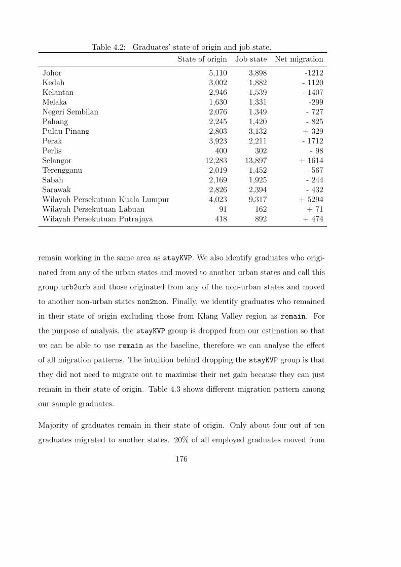
Table 4.2: Graduates’ state of origin and job state.
State of origin Job state Net migration
Johor 5,110 3,898 -1212Kedah 3,002 1,882 - 1120Kelantan 2,946 1,539 - 1407Melaka 1,630 1,331 -299Negeri Sembilan 2,076 1,349 - 727Pahang 2,245 1,420 - 825Pulau Pinang 2,803 3,132 + 329Perak 3,923 2,211 - 1712Perlis 400 302 - 98Selangor 12,283 13,897 + 1614Terengganu 2,019 1,452 - 567Sabah 2,169 1,925 - 244Sarawak 2,826 2,394 - 432Wilayah Persekutuan Kuala Lumpur 4,023 9,317 + 5294Wilayah Persekutuan Labuan 91 162 + 71Wilayah Persekutuan Putrajaya 418 892 + 474
remain working in the same area as stayKVP. We also identify graduates who origi-
nated from any of the urban states and moved to another urban states and call this
group urb2urb and those originated from any of the non-urban states and moved
to another non-urban states non2non. Finally, we identify graduates who remained
in their state of origin excluding those from Klang Valley region as remain. For
the purpose of analysis, the stayKVP group is dropped from our estimation so that
we can be able to use remain as the baseline, therefore we can analyse the effect
of all migration patterns. The intuition behind dropping the stayKVP group is that
they did not need to migrate out to maximise their net gain because they can just
remain in their state of origin. Table 4.3 shows different migration pattern among
our sample graduates.
Majority of graduates remain in their state of origin. Only about four out of ten
graduates migrated to another states. 20% of all employed graduates moved from
176

Table 4.3: Graduate migration patterns.
Item Number Per centnon2urb 7,980 21.39urb2urb 4,361 11.69non2non 2,320 6.22urb2non 850 2.28stayKVP 8,640 23.16remain 13,158 35.27Total 37,309 100.00
non-urban states to urban states. There are larger fraction of Law and Computer
Science graduates who move within the urban states urb2urb. A percentage of 2%
moved from an urban origin to non-urban states. Out of 850 graduates who reported
as urb2non, half of them were from Medical and Engineering. 12% moved from an
urban state to another and 5% moved from a non-urban state to another.
The cross tabulation between graduate income and migration pattern in Table 4.4
confirms our initial assumption that graduates who remain in their states (excluding
those from Klang Valley region) have more tendency of getting lower pay. There
may be several reasons for this. It could be because of their lower characteristics,
where they couldn’t compete with those who migrated out and hence they choose
to remain. It could be that they prefer to remain, at the cost of lower remuneration.
However we can’t say similar things to those who originated and remained employed
in Klang Valley region because they are more likely to earn middle income between
RM 1500 to RM 2500. Another pattern can be seen among those who migrated but
stay within the urban regions - half of these graduates earn a little bit higher than
those who remained in the Klang Valley, they earn between RM2000 to RM 3000.
We would expect graduates who moved from the non-urban states to show more ten-
dency towards the highest earning, instead our graduates sample show that those
177
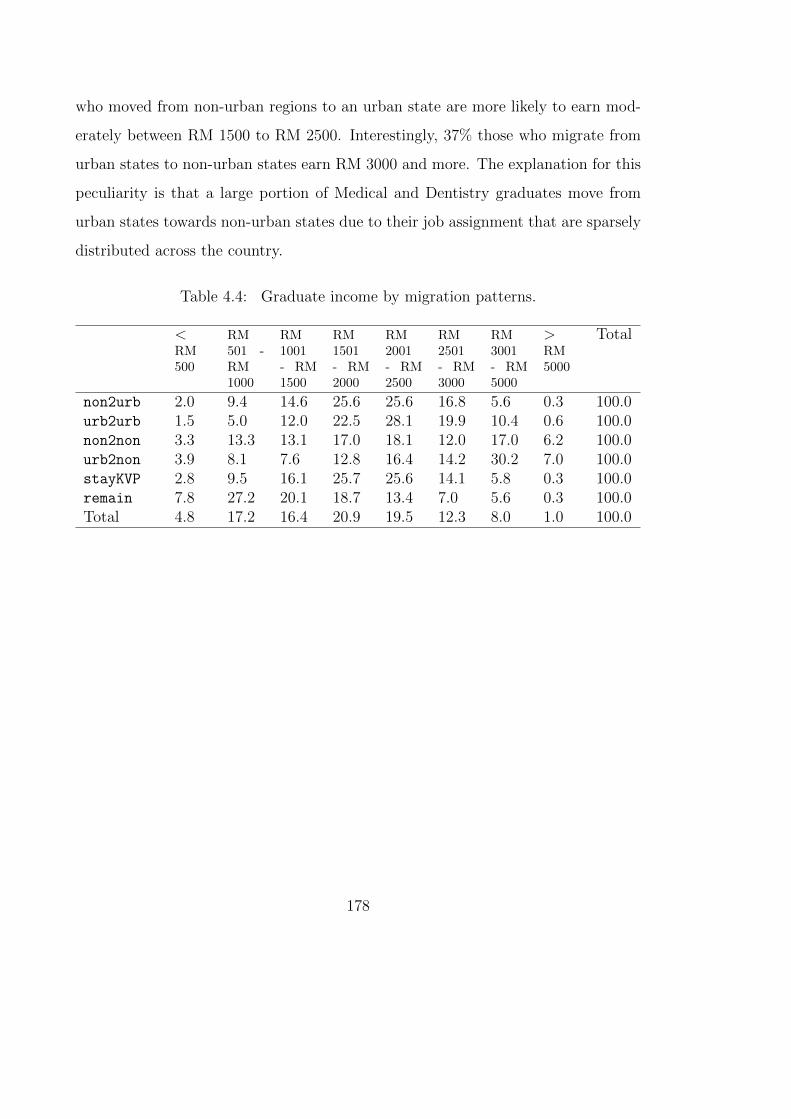
who moved from non-urban regions to an urban state are more likely to earn mod-
erately between RM 1500 to RM 2500. Interestingly, 37% those who migrate from
urban states to non-urban states earn RM 3000 and more. The explanation for this
peculiarity is that a large portion of Medical and Dentistry graduates move from
urban states towards non-urban states due to their job assignment that are sparsely
distributed across the country.
Table 4.4: Graduate income by migration patterns.
<RM500
RM501 -RM1000
RM1001- RM1500
RM1501- RM2000
RM2001- RM2500
RM2501- RM3000
RM3001- RM5000
>RM5000
Total
non2urb 2.0 9.4 14.6 25.6 25.6 16.8 5.6 0.3 100.0urb2urb 1.5 5.0 12.0 22.5 28.1 19.9 10.4 0.6 100.0non2non 3.3 13.3 13.1 17.0 18.1 12.0 17.0 6.2 100.0urb2non 3.9 8.1 7.6 12.8 16.4 14.2 30.2 7.0 100.0stayKVP 2.8 9.5 16.1 25.7 25.6 14.1 5.8 0.3 100.0remain 7.8 27.2 20.1 18.7 13.4 7.0 5.6 0.3 100.0Total 4.8 17.2 16.4 20.9 19.5 12.3 8.0 1.0 100.0
178

Table 4.5 presents the cross tabulation between graduate income and education-job
mismatch. Consistent with our assumption, education-job mismatch is related to
lower wage. The pattern of migration and education-job mismatch in Table 4.6
seems do not display any significant pattern.
Table 4.5: Graduate income by education-job (mis)match.
Graduate income Highlymatched
Matched Mis-matched
Highlymis-
matched
Total
< RM 500 24.9 47.7 20.9 6.5 100.0RM 501 - RM 1000 26.6 49.2 18.8 5.4 100.0RM 1001 - RM 1500 30.0 54.3 13.3 2.3 100.0RM 1501 - RM 2000 29.8 56.4 11.9 1.8 100.0RM 2001 - RM 2500 25.5 60.1 12.7 1.6 100.0RM 2501 - RM 3000 26.5 60.9 11.2 1.5 100.0RM 3001 - RM 5000 40.1 50.8 7.6 1.5 100.0> RM 5000 33.2 54.2 10.5 2.0 100.0Total 28.6 55.5 13.3 2.6 100.0
Table 4.6: Education-job (mis)match by migration patterns.
Highlymatched
Matched Mis-matched
Highlymis-
matched
Total
non2urb 27.7 57.4 12.9 2.0 100.0urb2urb 27.7 57.4 12.9 2.0 100.0non2non 29.7 55.9 12.4 1.9 100.0urb2non 38.4 49.9 10.1 1.6 100.0stayKVP 28.0 56.6 13.1 2.3 100.0remain 28.9 53.3 14.6 3.2 100.0Total 28.6 55.5 13.3 2.6 100.0
179
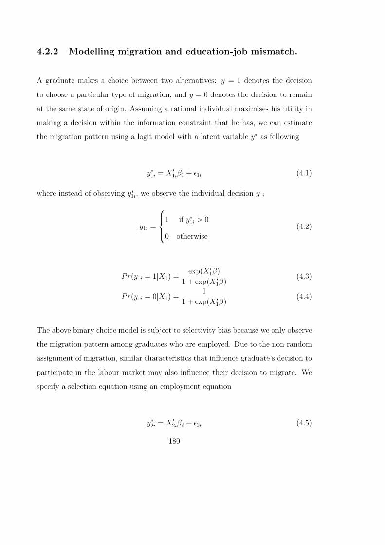
4.2.2 Modelling migration and education-job mismatch.
A graduate makes a choice between two alternatives: y = 1 denotes the decision
to choose a particular type of migration, and y = 0 denotes the decision to remain
at the same state of origin. Assuming a rational individual maximises his utility in
making a decision within the information constraint that he has, we can estimate
the migration pattern using a logit model with a latent variable y∗ as following
y∗1i = X ′1iβ1 + ε1i (4.1)
where instead of observing y∗1i, we observe the individual decision y1i
y1i =
1 if y∗1i > 0
0 otherwise
(4.2)
Pr(y1i = 1|X1) =exp(X ′1β)
1 + exp(X ′1β)(4.3)
Pr(y1i = 0|X1) =1
1 + exp(X ′1β)(4.4)
The above binary choice model is subject to selectivity bias because we only observe
the migration pattern among graduates who are employed. Due to the non-random
assignment of migration, similar characteristics that influence graduate’s decision to
participate in the labour market may also influence their decision to migrate. We
specify a selection equation using an employment equation
y∗2i = X ′2iβ2 + ε2i (4.5)
180
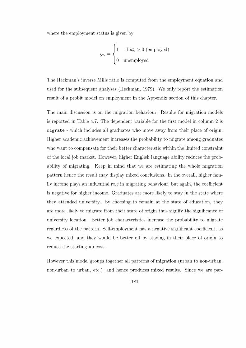
where the employment status is given by
y2i =
1 if y∗2i > 0 (employed)
0 unemployed
The Heckman’s inverse Mills ratio is computed from the employment equation and
used for the subsequent analyses (Heckman, 1979). We only report the estimation
result of a probit model on employment in the Appendix section of this chapter.
The main discussion is on the migration behaviour. Results for migration models
is reported in Table 4.7. The dependent variable for the first model in column 2 is
migrate - which includes all graduates who move away from their place of origin.
Higher academic achievement increases the probability to migrate among graduates
who want to compensate for their better characteristic within the limited constraint
of the local job market. However, higher English language ability reduces the prob-
ability of migrating. Keep in mind that we are estimating the whole migration
pattern hence the result may display mixed conclusions. In the overall, higher fam-
ily income plays an influential role in migrating behaviour, but again, the coefficient
is negative for higher income. Graduates are more likely to stay in the state where
they attended university. By choosing to remain at the state of education, they
are more likely to migrate from their state of origin thus signify the significance of
university location. Better job characteristics increase the probability to migrate
regardless of the pattern. Self-employment has a negative significant coefficient, as
we expected, and they would be better off by staying in their place of origin to
reduce the starting up cost.
However this model groups together all patterns of migration (urban to non-urban,
non-urban to urban, etc.) and hence produces mixed results. Since we are par-
181
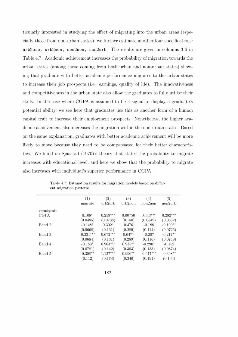
ticularly interested in studying the effect of migrating into the urban areas (espe-
cially those from non-urban states), we further estimate another four specifications:
urb2urb, urb2non, non2non, non2urb. The results are given in columns 3-6 in
Table 4.7. Academic achievement increases the probability of migration towards the
urban states (among those coming from both urban and non-urban states) show-
ing that graduate with better academic performance migrates to the urban states
to increase their job prospects (i.e. earnings, quality of life). The innovativeness
and competitiveness in the urban state also allow the graduates to fully utilise their
skills. In the case where CGPA is assumed to be a signal to display a graduate’s
potential ability, we see here that graduates use this as another form of a human
capital trait to increase their employment prospects. Nonetheless, the higher aca-
demic achievement also increases the migration within the non-urban states. Based
on the same explanation, graduates with better academic achievement will be more
likely to move because they need to be compensated for their better characteris-
tics. We build on Sjaastad (1970)’s theory that states the probability to migrate
increases with educational level, and here we show that the probability to migrate
also increases with individual’s superior performance in CGPA.
Table 4.7: Estimation results for migration models based on differ-ent migration patterns
(1) (2) (3) (4) (5)migrate urb2urb urb2non non2non non2urb
y=migrateCGPA 0.108∗ 0.259∗∗∗ 0.00750 0.443∗∗∗ 0.282∗∗∗
(0.0485) (0.0738) (0.150) (0.0849) (0.0552)Band 2 -0.148∗ 0.302∗ 0.476 -0.188 -0.190∗∗
(0.0668) (0.131) (0.289) (0.114) (0.0726)Band 3 -0.231∗∗∗ 0.672∗∗∗ 0.647∗ -0.207 -0.217∗∗
(0.0684) (0.131) (0.289) (0.116) (0.0749)Band 4 -0.183∗ 0.963∗∗∗ 0.935∗∗ -0.290∗ -0.152
(0.0781) (0.142) (0.303) (0.133) (0.0874)Band 5 -0.308∗∗ 1.127∗∗∗ 0.996∗∗ -0.677∗∗∗ -0.398∗∗
(0.112) (0.178) (0.340) (0.194) (0.133)
182

Band 6 0.165 1.772∗∗∗ 1.315∗ 0.0675 0.699(0.332) (0.495) (0.652) (0.563) (0.447)
Arts/SocSc -0.246 -0.249 1.674 -0.271 -0.514∗∗
(0.165) (0.229) (1.061) (0.334) (0.185)Transport 0.300 -0.292 1.980 -1.268 0.0133
(0.268) (0.385) (1.183) (0.787) (0.301)Administration -0.0271 -0.373 1.674 -0.0243 -0.255
(0.155) (0.207) (1.029) (0.313) (0.177)Management -0.234 -0.364 1.417 -0.142 -0.486∗∗
(0.150) (0.195) (1.027) (0.307) (0.170)Economy -0.0592 -0.518∗ 1.620 0.194 -0.281
(0.174) (0.255) (1.074) (0.334) (0.195)Accountancy -0.129 -0.283 1.006 -0.298 -0.332
(0.155) (0.201) (1.037) (0.317) (0.176)Marketing -0.372∗ -0.216 0.968 0.0942 -0.556∗∗
(0.182) (0.245) (1.131) (0.341) (0.204)Finance -0.105 -0.138 1.140 0.0148 -0.285
(0.156) (0.205) (1.049) (0.317) (0.177)Journalism 0.0463 0.847∗∗∗ 1.607 -0.612 0.177
(0.171) (0.219) (1.091) (0.405) (0.198)Islamic -0.00436 -0.910∗∗ 2.050 0.266 -0.257
(0.189) (0.306) (1.069) (0.355) (0.212)Food/hospitality -0.153 -0.121 2.159∗ -0.0949 -0.442∗
(0.180) (0.238) (1.049) (0.353) (0.204)Arts -0.000492 -0.127 1.889 -0.397 -0.262
(0.175) (0.252) (1.085) (0.371) (0.197)Pure science 0.0997 -0.167 1.497 -0.159 -0.162
(0.190) (0.273) (1.133) (0.395) (0.213)Applied science -0.216 -0.145 2.006 -0.196 -0.508∗∗
(0.156) (0.204) (1.029) (0.320) (0.177)Pharmacy -0.0615 0.0756 3.673∗∗∗ -0.992 -0.596
(0.303) (0.425) (1.116) (0.797) (0.362)Medical -0.0896 -1.949∗∗∗ 2.697∗∗ 0.142 -1.338∗∗∗
(0.175) (0.244) (1.039) (0.336) (0.210)Dentistry -0.461 -1.616∗∗ 3.746∗∗∗ -0.0636 -2.328∗∗∗
(0.388) (0.596) (1.114) (0.591) (0.649)Nurse 0.258 -0.105 2.133∗ -0.142 0.0101
(0.183) (0.251) (1.066) (0.391) (0.209)Environment -0.292 -0.768∗∗ 2.267∗ 0.517 -0.628∗∗
(0.176) (0.250) (1.041) (0.327) (0.200)Sports 0.530 -0.0180 2.884∗ -0.812 0.258
(0.275) (0.458) (1.182) (0.792) (0.310)Engineering 0.00554 -0.538∗∗ 2.082∗ 0.431 -0.233
(0.143) (0.186) (1.012) (0.297) (0.164)CompSci 0.488∗∗ 0.434∗ 1.782 0.161 0.559∗∗
(0.150) (0.197) (1.029) (0.315) (0.173)Education -0.690∗∗∗ -1.405∗∗∗ 1.810 0.0164 -1.103∗∗∗
183

(0.167) (0.245) (1.043) (0.321) (0.188)Male 0.0835∗ 0.237∗∗∗ 0.350∗∗∗ 0.343∗∗∗ 0.164∗∗∗
(0.0352) (0.0534) (0.0987) (0.0598) (0.0403)Age -0.0156 -0.00226 -0.109 -0.00727 -0.00100
(0.0196) (0.0293) (0.0588) (0.0342) (0.0222)Malay 0.502∗∗∗ 1.068∗∗∗ 0.355∗ 0.203∗ 0.749∗∗∗
(0.0585) (0.0946) (0.165) (0.0968) (0.0644)Chinese 0.593∗∗∗ 0.111 0.163 0.751∗∗∗ 0.758∗∗∗
(0.0750) (0.119) (0.207) (0.125) (0.0839)RM 501 - RM 1000 -0.0635 -0.243 -0.710∗∗∗ -0.160 -0.0876
(0.0671) (0.126) (0.213) (0.110) (0.0747)RM 1001 - RM 1500 -0.0560 0.0268 -0.389 -0.252∗ -0.0826
(0.0691) (0.125) (0.202) (0.113) (0.0772)RM 1501 - RM 2000 -0.107 0.167 -0.363 -0.266∗ -0.103
(0.0723) (0.127) (0.207) (0.118) (0.0813)RM 2001 - RM 2500 -0.171∗ 0.467∗∗∗ -0.238 -0.306∗ -0.145
(0.0763) (0.128) (0.214) (0.126) (0.0863)RM 2501 - RM 3000 -0.140 0.667∗∗∗ -0.342 -0.382∗∗ -0.0561
(0.0730) (0.123) (0.209) (0.124) (0.0826)RM 3001 - RM 5000 -0.254∗∗∗ 0.800∗∗∗ -0.253 -0.454∗∗∗ -0.143
(0.0733) (0.121) (0.204) (0.126) (0.0833)> RM 5000 -0.367∗∗∗ 1.152∗∗∗ 0.0431 -0.416∗∗ -0.166
(0.0822) (0.127) (0.211) (0.147) (0.0965)Unistay∗ 0.800∗∗∗ 0.530∗∗∗ -0.349∗∗ 0.0253 1.015∗∗∗
(0.0347) (0.0577) (0.134) (0.0699) (0.0401)Full time 0.542∗∗∗ 0.921∗∗∗ 0.326∗ 0.401∗∗∗ 0.731∗∗∗
(0.0494) (0.0813) (0.149) (0.0815) (0.0533)Permanent 0.0754∗ 0.0449 0.114 0.0696 0.104∗∗
(0.0343) (0.0516) (0.101) (0.0599) (0.0390)Professional 0.262∗∗∗ 0.520∗∗∗ 0.374∗∗ 0.252∗∗∗ 0.392∗∗∗
(0.0368) (0.0564) (0.118) (0.0636) (0.0404)Self-employed -1.113∗∗∗ -1.533∗∗∗ 0.179 -0.737∗∗∗ -1.671∗∗∗
(0.134) (0.223) (0.238) (0.189) (0.164)λ 0.393∗ -0.833∗∗ -1.502∗∗ -0.0301 0.443∗
(0.178) (0.269) (0.537) (0.309) (0.200)Constant -2.111∗∗ -4.055∗∗∗ -2.254 -3.560∗∗ -3.059∗∗∗
(0.668) (1.005) (2.206) (1.167) (0.757)
Observations 21952 13464 11302 12521 16768
Standard errors in parenthesesUnistay∗ = Obtain job at the state where they attended university.∗ p < 0.05, ∗∗ p < 0.01, ∗∗∗ p < 0.001
The results for English language score is more meaningful when we separate the
analysis by different migration pattern. Higher MUET score clearly increases mi-
184

gration of graduates within the urban states but it also increases the migration from
an urban state to a non-urban state. The peculiarity of the relationship between
higher English score and moving from an urban state to work in the non-urban
state can be explained by the courses of study. We found that at least seven out
of ten Medical and Dentistry graduates attained a MUET score of at least Band 3,
compared to the other graduates (except Law) who averages about three out of ten.
Medical and Dentistry graduates also have the highest fraction of graduates who
move from an urban state to non-urban states (15% of Medical and 23% of Den-
tistry), compared to the average of all other graduates at 2.9%. The explanation of
higher MUET and choosing to move from an urban state to a non-urban state must
therefore be taken with precaution. On the other hand, graduates who scored Band
2, Band 3, and Band 5 reduces the migration pattern from a non-urban state to an
urban state. Similarly, Band 4 and Band 5 graduates reduces non2non migration.
One explanation is that due to the competitiveness in the urban job market, grad-
uates with better signalling (both CGPA and MUET) have better chance to obtain
jobs in the urban state, pushing the remaining with lower CGPA and lower MUET
score to work in the non-urban states.
We use Law as the base category to discuss the effect of courses of study. Journalism
and Computer Science graduates are much more likely to choose urb2urb migra-
tion. Courses such as Economy and Engineering are less likely than Law, but their
pattern to choose urb2urb is higher than the rest. For urb2non migration we found
mostly the graduates who took Science subjects5 are more likely to migrate in this
pattern. 60% of Pharmacy graduates, 84% of Medical graduates, and 93% of Den-
tistry graduates work with the public sector which randomly assign them towards
more sparsely distributed job location across the country. We also found that Engi-
neering and Food & Hospitality are also more likely to move urb2non. Engineering
5Pharmacy, Medical, Dentistry, Nurse, Environment, Sports
185
graduates constitute the largest group in our sample, a quarter of all the observed
graduates. The migration pattern of Engineering graduates who are more likely to
choose urb2non can perhaps be explained by the competition dimply because there
are a lot of Engineering graduates in the market and the jobs availability in the
urban states are limited.
We found none of the courses of study are significantly different than Law in the case
of migration from a non-urban state to another. For non2urb, again, Medical, Den-
tistry, and Education graduates are less likely to choose this migration pattern - on
account of their employment with the public sector (hospitals, health departments,
schools) that allocate them more sparsely into the larger region of non-urban states.
In contrast, Computer Science graduates are more likely to move from a non-urban
state to an urban state which corresponds to the availability of high technological
jobs in the more developed states.
Male graduates are more likely to migrate in all migration circumstances, which
may help explain their better remuneration and job characteristics. Women, on the
other hand, are less likely to move and rather remain at the state of origin. Age
has no significant effect on graduates’ migration. The result for age in this sample
should not be generalised to the larger sample because we only observe a homoge-
nous group of youth in their early careers. We further look at the contribution
of family income. Higher family income increases the migration within the urban
states, understandably due to the costs associated with migration, and particularly,
migrating towards urban states require higher costs of living. However, higher fam-
ily income reduces the migration within the non-urban states. Graduates among the
lowest family income may choose to migrate within the non-urban states so they
can increase their employment prospects better than staying. Compared to all the
other ethnic groups, Malays are more likely to migrate in all directions. Chinese’s
186

coefficients are only significant in the migration from the non-urban states - signify
the movement patterns of Chinese towards the urban states. The coefficients of
Chinese migration from the urban states are not significant.
As we have expected, those who attended universities in an urban state are more
likely to migrate from their state of origin and stay at the location of their study.
The place of education is found to be a strong link for migration behaviour - those
who choose to study at an urban institution tend to stay there for employment,
conversely, those who studied at non-urban areas did not choose to stay. The result
is similar to the Italian graduates (Iammarino and Marinelli, 2007) in which grad-
uates who attended universities in the urban areas are more likely to be absorbed
by the local labour market. There is some correlation between attending selective
universities in the urban areas and high ability graduates. This is because the top
universities are located in the urban states6. More prestigious universities choose
potential applications from a pool of high school leavers who scored exceptional
achievements. These highly competitive students possess better attributes to per-
form well in those selective institutions and then perform better to secure superior
occupations after graduating. Regardless of where they come from, these graduates
who have already resided in an urban state during their study have already accus-
tomed themselves to those states and hence making the transition to obtain a job in
those states is much easier than those who attend institutions in non-urban states.
The correlation between migration and high ability graduates creates an endogene-
ity problem where only those with high expectation for higher income coupled with
the higher confidence that they can do better (due to their better quality) will move.
This opens up an opportunity for new research using an appropriate instrument to
handle the endogeneity issue created by the sorting algorithm.
6Top public universities such as UM, UKM, and UPM are located in the Klang Valley; USM inPenang; and all renowned private institutions are located in Klang Valley.
187

This finding suggests that an urban state may continuously creating a self-reinforcing
mechanism in which they offer education for skills creation, and at the same time
offer jobs to utilise those skills, thus making an urban state continues to grow while
leaving the remaining states losing out both in terms of retaining skills and growth.
Our analysis shows that better job characteristics are associated with all migrating
patterns, which only strengthen our assumption that graduates choose to migrate
to obtain better jobs. As we have expected, the self-employed are less likely to
move into another state in all model (except urb2non where the coefficient is not
significant).
188

Education-job mismatch and migration.
Turning to the core research question on the impact of migration towards education-
job (mis)match. Consider the model of education-job mismatch in an ordered depen-
dent variable of a 4-Likert scales from 1:highly matched to 4:highly mismatched
listed in the Table 4.1. The model can be estimated by a latent variable y∗i = X ′β+ε
where the observed variable y is related to the latent variable as y = 1(y∗ ≤ j) with
j = 1, 2, 3, 4 denotes the four levels of education-job (mis)match. Let α1 < α2 < α3
be the threshold parameters to be estimated with β where
y = 1 if y∗ ≤ α1
y = 2 if α1 < y∗ ≤ α2
y = 3 if α1 < y∗ ≤ α3
y = 4 if y∗ > α3
Then, the response probability is defined as
Pr(y = j) = Λ(αj −X ′β) (4.6)
where Λ(.) is a logistic function. A set of factors such as SES variables, education,
and job characteristics, may explain the education-job (mis)match. We take into
account the selectivity bias by including the inverse Mills ratio from the employment
equation, which is reflected in the λ coefficient in the estimation result.
The results of an ordered model are presented in Table 4.8 for four regions: Klang
Valley and Penang (KVP), North and South, Borneo, and Eastern states. The
189
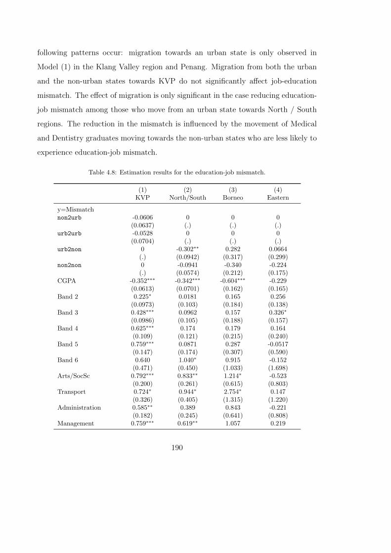
following patterns occur: migration towards an urban state is only observed in
Model (1) in the Klang Valley region and Penang. Migration from both the urban
and the non-urban states towards KVP do not significantly affect job-education
mismatch. The effect of migration is only significant in the case reducing education-
job mismatch among those who move from an urban state towards North / South
regions. The reduction in the mismatch is influenced by the movement of Medical
and Dentistry graduates moving towards the non-urban states who are less likely to
experience education-job mismatch.
Table 4.8: Estimation results for the education-job mismatch.
(1) (2) (3) (4)KVP North/South Borneo Eastern
y=Mismatchnon2urb -0.0606 0 0 0
(0.0637) (.) (.) (.)urb2urb -0.0528 0 0 0
(0.0704) (.) (.) (.)urb2non 0 -0.302∗∗ 0.282 0.0664
(.) (0.0942) (0.317) (0.299)non2non 0 -0.0941 -0.340 -0.224
(.) (0.0574) (0.212) (0.175)CGPA -0.352∗∗∗ -0.342∗∗∗ -0.604∗∗∗ -0.229
(0.0613) (0.0701) (0.162) (0.165)Band 2 0.225∗ 0.0181 0.165 0.256
(0.0973) (0.103) (0.184) (0.138)Band 3 0.428∗∗∗ 0.0962 0.157 0.326∗
(0.0986) (0.105) (0.188) (0.157)Band 4 0.625∗∗∗ 0.174 0.179 0.164
(0.109) (0.121) (0.215) (0.240)Band 5 0.759∗∗∗ 0.0871 0.287 -0.0517
(0.147) (0.174) (0.307) (0.590)Band 6 0.640 1.040∗ 0.915 -0.152
(0.471) (0.450) (1.033) (1.698)Arts/SocSc 0.792∗∗∗ 0.833∗∗ 1.214∗ -0.523
(0.200) (0.261) (0.615) (0.803)Transport 0.724∗ 0.944∗ 2.754∗ 0.147
(0.326) (0.405) (1.315) (1.220)Administration 0.585∗∗ 0.389 0.843 -0.221
(0.182) (0.245) (0.641) (0.808)Management 0.759∗∗∗ 0.619∗∗ 1.057 0.219
190

(0.175) (0.239) (0.602) (0.789)Economy 1.075∗∗∗ 0.518 1.216 -0.163
(0.216) (0.269) (0.644) (0.819)Accountancy 0.238 0.210 0.627 0.00437
(0.179) (0.246) (0.623) (0.809)Marketing 0.225 0.199 0.339 -0.286
(0.218) (0.274) (0.627) (0.854)Finance 0.601∗∗ 0.461 0.938 0.335
(0.183) (0.248) (0.615) (0.804)Journalism 0.557∗∗ 0.282 1.152 -0.605
(0.195) (0.287) (0.684) (0.866)Islamic 0.624∗ 0.177 0.463 0.140
(0.251) (0.284) (0.762) (0.815)Food/hospitality 0.373 0.325 0.692 -0.795
(0.218) (0.281) (0.634) (0.855)Arts 0.690∗∗ 1.038∗∗∗ 1.557∗ 0.0233
(0.217) (0.290) (0.634) (0.818)Pure science 1.454∗∗∗ 1.082∗∗∗ 2.378∗∗ 0.697
(0.226) (0.312) (0.799) (0.849)Applied science 1.240∗∗∗ 1.120∗∗∗ 1.606∗∗ 0.788
(0.183) (0.249) (0.609) (0.802)Pharmacy 0.415 0.422 -0.886 -0.543
(0.398) (0.443) (1.332) (1.129)Medical -0.594∗∗ -0.103 0.987 0.134
(0.228) (0.269) (0.659) (0.849)Dentistry 0.797 0.0559 0.0692 -1.507
(0.774) (0.493) (1.300) (1.350)Nurse 0.134 0.822∗∗ 0.870 -0.441
(0.219) (0.310) (0.723) (0.856)Environment 0.729∗∗ 1.015∗∗∗ 1.410∗ 0.585
(0.226) (0.266) (0.660) (0.822)Sports 0.571 0.873 1.389 2.261
(0.362) (0.447) (1.257) (1.200)Engineering 0.820∗∗∗ 1.027∗∗∗ 1.720∗∗ 0.646
(0.165) (0.233) (0.590) (0.786)CompSci 0.863∗∗∗ 0.914∗∗∗ 1.455∗ 0.588
(0.172) (0.250) (0.628) (0.813)Education 0.606∗∗ 0.228 0.609 -0.257
(0.209) (0.253) (0.616) (0.801)Male -0.0839 -0.166∗∗ -0.141 0.340∗∗
(0.0453) (0.0511) (0.106) (0.112)Age -0.0639∗ -0.128∗∗∗ -0.0298 -0.0296
(0.0254) (0.0284) (0.0584) (0.0603)Malay 0.0909 -0.0577 -0.249∗ -0.684
(0.0862) (0.100) (0.120) (0.475)Chinese 0.669∗∗∗ 0.717∗∗∗ 0.839∗∗∗ 0.424
(0.105) (0.119) (0.172) (0.549)
191
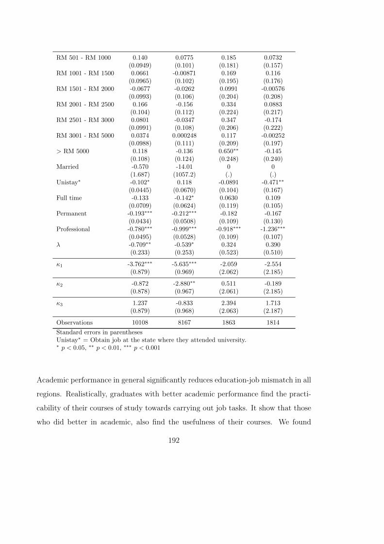
RM 501 - RM 1000 0.140 0.0775 0.185 0.0732(0.0949) (0.101) (0.181) (0.157)
RM 1001 - RM 1500 0.0661 -0.00871 0.169 0.116(0.0965) (0.102) (0.195) (0.176)
RM 1501 - RM 2000 -0.0677 -0.0262 0.0991 -0.00576(0.0993) (0.106) (0.204) (0.208)
RM 2001 - RM 2500 0.166 -0.156 0.334 0.0883(0.104) (0.112) (0.224) (0.217)
RM 2501 - RM 3000 0.0801 -0.0347 0.347 -0.174(0.0991) (0.108) (0.206) (0.222)
RM 3001 - RM 5000 0.0374 0.000248 0.117 -0.00252(0.0988) (0.111) (0.209) (0.197)
> RM 5000 0.118 -0.136 0.650∗∗ -0.145(0.108) (0.124) (0.248) (0.240)
Married -0.570 -14.01 0 0(1.687) (1057.2) (.) (.)
Unistay∗ -0.102∗ 0.118 -0.0891 -0.471∗∗
(0.0445) (0.0670) (0.104) (0.167)Full time -0.133 -0.142∗ 0.0630 0.109
(0.0709) (0.0624) (0.119) (0.105)Permanent -0.193∗∗∗ -0.212∗∗∗ -0.182 -0.167
(0.0434) (0.0508) (0.109) (0.130)Professional -0.780∗∗∗ -0.999∗∗∗ -0.918∗∗∗ -1.236∗∗∗
(0.0495) (0.0528) (0.109) (0.107)λ -0.709∗∗ -0.539∗ 0.324 0.390
(0.233) (0.253) (0.523) (0.510)
κ1 -3.762∗∗∗ -5.635∗∗∗ -2.059 -2.554(0.879) (0.969) (2.062) (2.185)
κ2 -0.872 -2.880∗∗ 0.511 -0.189(0.878) (0.967) (2.061) (2.185)
κ3 1.237 -0.833 2.394 1.713(0.879) (0.968) (2.063) (2.187)
Observations 10108 8167 1863 1814
Standard errors in parenthesesUnistay∗ = Obtain job at the state where they attended university.∗ p < 0.05, ∗∗ p < 0.01, ∗∗∗ p < 0.001
Academic performance in general significantly reduces education-job mismatch in all
regions. Realistically, graduates with better academic performance find the practi-
cability of their courses of study towards carrying out job tasks. It show that those
who did better in academic, also find the usefulness of their courses. We found
192
an unexpected output for MUET score which shows graduates with higher MUET
(Band 2 - Band 5) are more likely to experience education-job mismatch in the
case of KVP region. What is more interesting however, this finding is especially
true among the private sector workers. Even though higher MUET score lead to
better occupational types and higher earning, MUET does not necessarily affect the
usefulness of courses of study in the job sector.
Using Law as the base category, we found a larger number of courses taken by
graduates working in the KVP region that are associated with significant tendency
to obtain jobs that do not match with their specialised qualification. Only Medical
courses significantly reduce the probability to obtain a mismatched job. Among the
courses that have the highest impact on increasing education-job mismatch in all
regions are generally: Pure Science, Applied Science, Engineering, and Computer
Science. In Eastern region, none of the courses are significantly different than Law,
but Applied Science, Pure Science, Engineering, and Computer Science consistently
have the largest impact (although non-significant). We analyse the incidence of an
education-job mismatch with precaution because there are various ways to measure
education-job mismatch and over-education. Since we use a secondary data from the
Graduate Tracer Study provided by the ministry, we have no control to construct a
question that can precisely differentiate between the incidence of over- and under-
education. Graduates’ response to the question if their qualification helps in their
current job may have a mixed combination of the two categories of mismatch.
Nonetheless, we discuss the influence of SES variables towards education-job mis-
match. Higher age significantly reduces the mismatch in the KVP and the North
/ South regions. Malays are less likely to be mismatched if they work in Borneo
regions. Chinese are experiencing significant education-job mismatch in all the three
regions excluding the Eastern state (because Chinese are less likely to be originated
193
from the Eastern states). Family income does not have any significant impact ex-
cept in the case of the Borneo region where the highest family income increases the
incidence of education-job mismatch. The impact of staying in the state where a
graduate attends their university reduces job mismatch in the KVP and the Eastern
states, intuitively because urban states consist of more selective universities attended
by better quality graduates. These graduates find the practicable usefulness of their
courses of study. Professional jobs significantly reduce job mismatch in all regions,
but full-time and permanent jobs show a more mixed findings.
The results are very mixed, partly considering the inadequacy of the question to
capture the distinction between over-education and under-education. Nonetheless,
graduates’ self-assessment on how helpful their courses are towards carrying out
their job tasks may explain who benefits most from their education by looking at the
contrast of the above results. Medical and Dentistry graduates are found to benefit
most because their courses of study are tailored to the market demand for highly
specialised skill in their field. Other courses are reported to have a lower degree of
practical usefulness of their degree towards carrying our their job tasks. The high
mismatch in courses such as Arts and Social Science is expected due to their varying
nature of practicability. However, the biggest concern is among the more attractive
and highly technical courses such as Engineering and Computer Science graduates
who have a similar pattern of a mismatch with the other courses. In another aspect,
CGPA and MUET are not significant in the model, hence suggesting that there is
no difference between the high scorer and the low scorer in terms of benefitting from
their education. However, graduates who work in professional job groups reported
a significant positive effect on the usefulness of their education towards their jobs.
194

The effect of migration on income.
Consider individual anticipated wage at current location is W ∗s and their anticipated
wage if move to new location is W ∗m as given in the following
W ∗s = Z ′sβs + us (4.7)
W ∗m = Z ′mβm + um (4.8)
Say the one-time cost of migration is C∗ = Z ′cβc + uc and the average realisable
earning gain across individual is given by ∆∗ = W ∗m −W ∗
s (Tunali, 2000)(Greene,
2000). The systematic sorting / migrating decision M = 1(W ∗m −W ∗
s − C∗ > 0)
is made on the basis of whether W ∗m − W ∗
s is larger than the costs of migrating.
However note that ∆∗ > 0 is not necessary condition for migration to take place.
M∗ = W ∗m −W ∗
s − C∗ (4.9)
= Z ′mβm − Z ′sβs − Z ′cβc + (um − us − uc) (4.10)
= X ′β + ε (4.11)
where a graduate’s choice to migrate is denoted as M = 1(M∗ > 0) which is in-
fluenced by the explanatory variables X. If the factors affecting employment also
affect migration decision, then we must take into account selectivity issues (Heck-
man, 1979). Thus, first we estimate employment equation where we calculate the
inverse Mills ratio and included it in the second step to estimate the earning equa-
tion.
195

We only report the effect of migration as presented in Table 4.9. The baseline
category is remain. The overall impact of migration in all regions are positive
and significant, signifies that by moving to another state regardless of origin or
destination being urban or not, increases graduates income, although it does not
have same effect on education-job (mis)match. This confirms our expectation that
graduates may move out of their state of origin to another states to maximise their
earnings regardless of whether the job matches with their qualification. We also
look at the effect of staying at the same location as the university. Surprisingly, we
found that the effect of working at the same state as the university reduces income
among those working in KVP and North/South regions.
Table 4.9: Estimation results for modelling the migration effect ongraduate income.
(1) (2) (3) (4)KVP North/South Borneo Eastern
y=Graduate incomenon2urb 0.562∗∗∗ 0 0 0
(0.0590) (.) (.) (.)urb2urb 0.805∗∗∗ 0 0 0
(0.0653) (.) (.) (.)urb2non 0 0.787∗∗∗ 1.247∗∗∗ 0.650∗
(.) (0.0900) (0.310) (0.302)non2non 0 0.830∗∗∗ 0.774∗∗∗ 0.890∗∗∗
(.) (0.0550) (0.204) (0.175)Unistay∗ -0.177∗∗∗ -0.253∗∗∗ -0.0676 -0.280
(0.0412) (0.0620) (0.0986) (0.169)
Observations 10108 8167 1863 1814
Standard errors in parenthesesUnistay∗ = Obtain job at the state where they attended university.∗ p < 0.05, ∗∗ p < 0.01, ∗∗∗ p < 0.001
196

4.2.3 Summary on migration pattern and education-job mis-
match.
The empirical findings on the effect of migration on education-job mismatch and
earning may be summarised by three broad conclusions. First, higher ability gradu-
ates are more likely to migrate and their migration reflects in their higher earnings.
Second, better job characteristics are associated with all migrating patterns, which
only strengthen our assumption that graduates choose to migrate to obtain better
jobs and to compensate for their higher ability (human capital). Third, migration
does not necessarily reduce education-job mismatch especially among some attrac-
tive courses such as Engineering and Computer Science. The finding informs us that
these graduates reported that their courses of study were not helpful in their current
job. On the surface, this finding may indicate the lack of quality in the teaching
of Engineering and Computer Science courses in Malaysian universities, but a more
accurate measure of education-job match is necessary to make a conclusion of the
usefulness of these courses offered in the country. The model however clearly dis-
tinguishes Medical and Dentistry graduates who were found to benefit the most
from their education. This is not surprising since their training is highly specialised
towards the needs of their labour market.
In the next section, we look at another dimension of graduate’s transition from
education to work by investigating the determinants influencing the time it took to
obtain their first job.
197
4.3 Transition time from higher education to em-
ployment.
Despite the occupational adjustment in the labour market to cater for the increasing
supply of graduates, the unemployment rate among university graduates is still very
high and their transition from university to work is distinctly long. Due to the
significant increases in the tertiary education, we may find newer cohorts facing
difficulties in securing jobs after spending years of education, and they took much
longer time to settle down on a job, compared to university graduates several years
back. Considering university education is a long and expensive investment, longer
transition period can be both devastating to graduates’ labour market opportunity
and motivation.
Graduates’ job search duration has become longer and is less defined now than
before. Longer job search period may have a direct effect on the graduate’s earnings
- in some cases due to prolonged unemployment, some graduates may opt to lower
their reservation wages. Some graduates, due to the difficulty to find a proper job,
coupled with the stress to pay up the education loan, may choose to lower their
expectation after some period elapsed and took up any jobs available, which may
result in over-qualification and being under-paid. By taking too long to start work,
they also lose in terms of skill accumulation that is necessary for a subsequent job
opportunity and remain at the back of the line compared to graduates who already
spent a longer time in employment.
In the first chapter, we have established the factors that lead to graduates successful
transition from university to work. However, the distribution of the length of dura-
tion to obtain the first job itself it rather interesting. Hence, this section is devoted
to understand the factors that lead to shorter or longer job search period until a
198
graduate land on his first job. The period of job search is characterised by the time
it took between finishing study and the time that the tracer study was conducted
during convocation. Obviously, there are still some graduates who remained unem-
ployed when the measure is taken, which causes some observation to be regarded as
censored.
Considering graduates’ first job have a significant impact on their subsequent tran-
sition in the labour market, it is important to understand what causes the long
job search duration. An interesting question to be asked is can it be plausible to
say that the longer the unemployment period, the harder for that individual to
get employed? Among graduates who remained unemployed several months after
graduation, what is the likelihood that the event (unemployment) will end in the
next period for individuals who have lasted that long? Are there factors affecting
the shorter/longer job search duration that can be explained by graduates’ choice
of education or simply due to their characteristics such as SES factors, academic
performance, and English language ability?
The screening hypothesis states that employers use cheaply observed characteristics
such as sex, ethnic group, academic performance, and course of study (some of
which is believed to correlate with productivity) during recruitment (Arrow, 1973).
Employers prefer those with superior characteristics, leaving job seekers with less
attractive attributes remained unemployed and have longer transition compared to
those with more attractive attributes. The job search theory states that both workers
and jobs are heterogenous - therefore, information about them becomes valuable and
hence, both employers and job seekers spend time and money in order to acquire
that information. Some graduates may refrain from accepting the first job offers
they received if they think they can do better in maximising their expected lifetime
earnings (Fallon and Verry, 1988). We will see later that Medical, Dentistry, and
199
Engineering graduates in this study show their tendency to delay working due to this
particular reason, considering their first job plays an important role for a subsequent
job in their career path. For Medical and Dentistry, their prolonged transition may
also be explained by their waiting for placement at one of the public organisations
which are scattered all over the country. Our data shows that longer transition is
also associated with public sector employment. We suspect that graduates who seek
employment with a larger firm such as multinational companies (MNC) may prolong
their employment due to the fact that MNC generally offers jobs at a certain time
within a year, but the data shows that there is no difference in the transition time
between those seeking employment with the MNC with those seeking job elsewhere.
4.3.1 Survival analysis of transition.
Appropriate method to model duration data is survival analysis. The duration is
defined as the time elapsed until a transition occur i.e. the event of employment.
The model was originally used in the medical field to analyse patient’s mortality
rate, hence called ‘survival’, but it is now widely applied in econometric settings
such as the study of unemployment duration. The dependent variable of interest
is the length of time that elapsed beginning from the time of finishing study until
the time the measurement is taken (survey) which may precede termination among
those who remain unemployed at the time the survey is conducted.
Given that an individual have remained unemployed until time t, let T ≥ 0 be the
length of time before the first spell of employment took place. The probability that
the respondent will be employed in the next short interval of time is given by a
200
hazard rate
λ(t) = limh→0
Pr(t ≤ T ≤ t+ h|T ≥ t)
h(4.12)
where λ(t) is the hazard function at which the spells are completed after duration
t and h is a small change in t. However the limitation of the above function is
that it does not take into consideration the effect of covariates that may explain the
transition process itself.
Indeed, we are more interested in the hazard function conditional on a set of covari-
ates X which is available for each individual and may have the predictive capability
of an individual subsequent failure time. Thus the hazard function is defined condi-
tional on the covariates. One way is to estimate an accelerated failure time (AFT)
model which allows for non-monotonic hazard function. We may assume that the
longer the unemployment spell, the less of a risk that the individual will remain
unemployed in the next short time period. This may due to several reasons. The
longer an individual spent in their job search, the more information they gain about
employment. Due to their longer wait, they may also reduce their reservation wage
by widening up their range of occupational choices. Considering majority of the
graduates took a study loan, they may feel an urge to seize any employment op-
portunity to be able to pay up the debt. There may be circumstances where an
individual may be more susceptible to remain unemployed after a long spell of un-
employment due to preference (i.e. married, child-bearing) or loss of motivation
(Salas-Velasco, 2007).
However, because parametric approach requires a certain degree of structure impo-
sition for modelling the distribution of baseline hazard which if not specified cor-
rectly may distort the estimated hazard rate (see Greene (2000) Ch. 19 pp. 909).
201
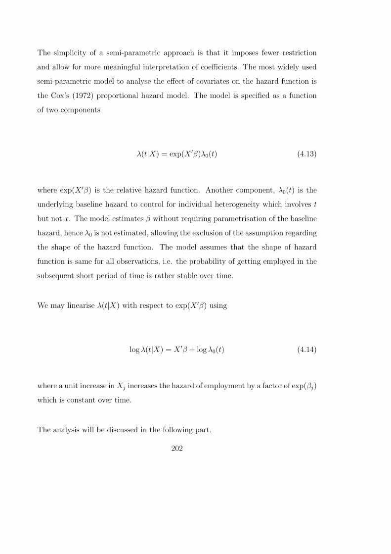
The simplicity of a semi-parametric approach is that it imposes fewer restriction
and allow for more meaningful interpretation of coefficients. The most widely used
semi-parametric model to analyse the effect of covariates on the hazard function is
the Cox’s (1972) proportional hazard model. The model is specified as a function
of two components
λ(t|X) = exp(X ′β)λ0(t) (4.13)
where exp(X ′β) is the relative hazard function. Another component, λ0(t) is the
underlying baseline hazard to control for individual heterogeneity which involves t
but not x. The model estimates β without requiring parametrisation of the baseline
hazard, hence λ0 is not estimated, allowing the exclusion of the assumption regarding
the shape of the hazard function. The model assumes that the shape of hazard
function is same for all observations, i.e. the probability of getting employed in the
subsequent short period of time is rather stable over time.
We may linearise λ(t|X) with respect to exp(X ′β) using
log λ(t|X) = X ′β + log λ0(t) (4.14)
where a unit increase in Xj increases the hazard of employment by a factor of exp(βj)
which is constant over time.
The analysis will be discussed in the following part.
202

4.3.2 The transition from university to work in Malaysia.
The graduates were asked about the length (in months) of their job search period
before they obtain first employment after graduation. Nevertheless, some obser-
vations are censored due to the on-going process of job search while the study is
conducted, leaving some respondents remained unemployed at the time they an-
swered the questionnaire. Table 4.10 display the frequency of employment spell
among our graduates. Within a twelve months timeframe, around 55% of the grad-
uate was reported to be employed. More than 80% among those whose employment
spell occurred at the time the survey is conducted were employed within the first
three months after graduation.
The average month it took for employed graduates from a different course of study
to obtain their first job is shown in Table 4.11. The overall waiting period is 2.18
months. Graduates from Arts, Sports, Transportation, and Environment were re-
ported to have the fastest transition from university to work. As a matter of fact,
graduates who studied Transportation do not only display the fastest transition to
work, 70% of them were reported to be employed when the survey is conducted.
At the end of another spectrum, graduates from Dentistry, Pharmacy, Medical,
and Education are reported to have the longest average waiting period, consistent
with our assumption that these graduates refrain from accepting their first job offer
when they think they can do better. They are followed by graduates who stud-
ied Education, Islamic, Management, and Engineering. Medical graduates are the
most employable, but they are among those who spent the longest in the search
period. Analysis later will show that professional and permanent job have a longer
transition. Hence it is reasonable that Medical, Dentistry, Engineering take longer
to obtain their first job because of their bias towards a permanent or professional
position.
203
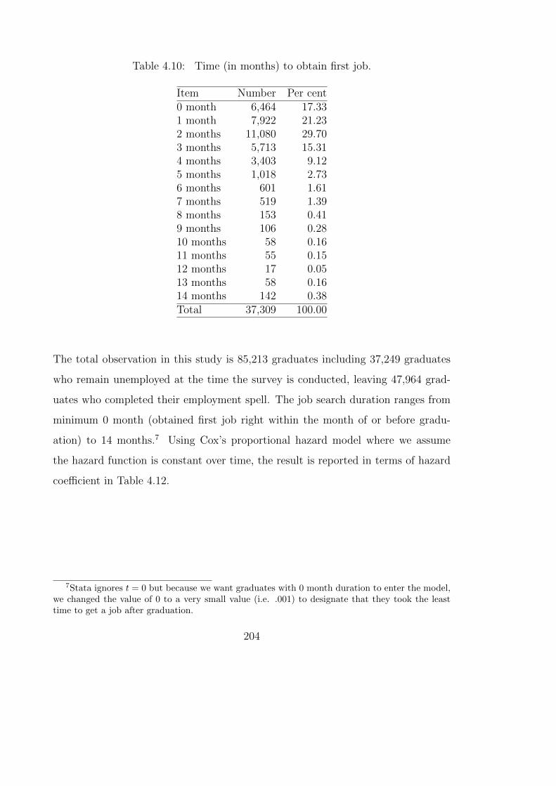
Table 4.10: Time (in months) to obtain first job.
Item Number Per cent0 month 6,464 17.331 month 7,922 21.232 months 11,080 29.703 months 5,713 15.314 months 3,403 9.125 months 1,018 2.736 months 601 1.617 months 519 1.398 months 153 0.419 months 106 0.2810 months 58 0.1611 months 55 0.1512 months 17 0.0513 months 58 0.1614 months 142 0.38Total 37,309 100.00
The total observation in this study is 85,213 graduates including 37,249 graduates
who remain unemployed at the time the survey is conducted, leaving 47,964 grad-
uates who completed their employment spell. The job search duration ranges from
minimum 0 month (obtained first job right within the month of or before gradu-
ation) to 14 months.7 Using Cox’s proportional hazard model where we assume
the hazard function is constant over time, the result is reported in terms of hazard
coefficient in Table 4.12.
7Stata ignores t = 0 but because we want graduates with 0 month duration to enter the model,we changed the value of 0 to a very small value (i.e. .001) to designate that they took the leasttime to get a job after graduation.
204
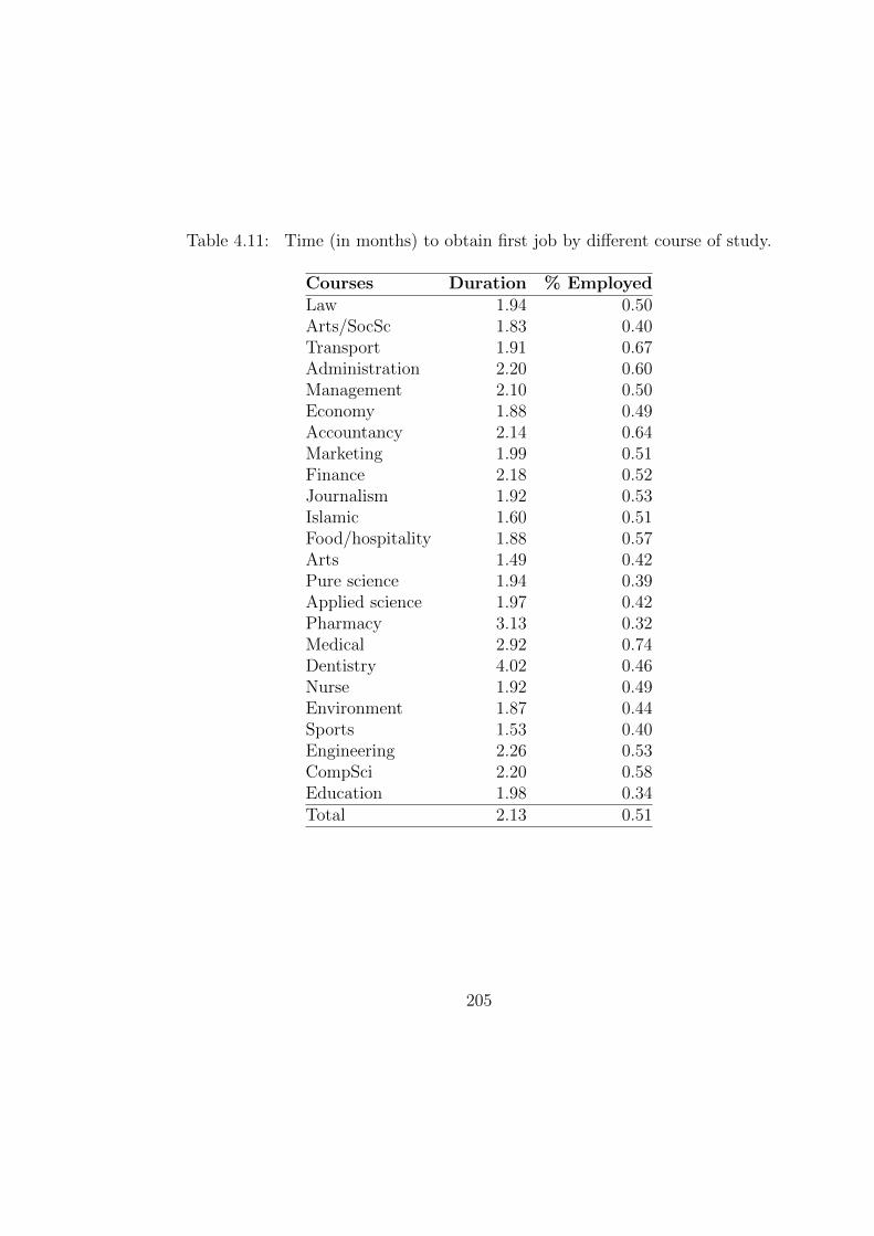
Table 4.11: Time (in months) to obtain first job by different course of study.
Courses Duration % EmployedLaw 1.94 0.50Arts/SocSc 1.83 0.40Transport 1.91 0.67Administration 2.20 0.60Management 2.10 0.50Economy 1.88 0.49Accountancy 2.14 0.64Marketing 1.99 0.51Finance 2.18 0.52Journalism 1.92 0.53Islamic 1.60 0.51Food/hospitality 1.88 0.57Arts 1.49 0.42Pure science 1.94 0.39Applied science 1.97 0.42Pharmacy 3.13 0.32Medical 2.92 0.74Dentistry 4.02 0.46Nurse 1.92 0.49Environment 1.87 0.44Sports 1.53 0.40Engineering 2.26 0.53CompSci 2.20 0.58Education 1.98 0.34Total 2.13 0.51
205
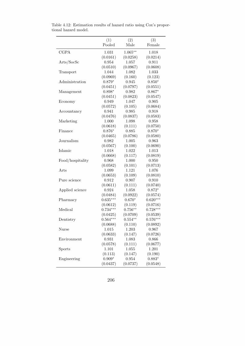
Table 4.12: Estimation results of hazard ratio using Cox’s propor-tional hazard model.
(1) (2) (3)Pooled Male Female
CGPA 1.031 1.065∗∗ 1.018(0.0161) (0.0258) (0.0214)
Arts/SocSc 0.954 1.057 0.911(0.0510) (0.0967) (0.0608)
Transport 1.044 1.082 1.033(0.0969) (0.160) (0.123)
Administration 0.879∗ 0.945 0.850∗
(0.0451) (0.0797) (0.0551)Management 0.898∗ 0.982 0.867∗
(0.0451) (0.0823) (0.0547)Economy 0.949 1.047 0.905
(0.0572) (0.105) (0.0684)Accountancy 0.941 0.985 0.918
(0.0476) (0.0837) (0.0583)Marketing 1.000 1.098 0.958
(0.0618) (0.111) (0.0750)Finance 0.876∗ 0.885 0.870∗
(0.0465) (0.0786) (0.0580)Journalism 0.982 1.005 0.963
(0.0567) (0.100) (0.0690)Islamic 1.018 1.022 1.013
(0.0668) (0.117) (0.0819)Food/hospitality 0.968 1.000 0.950
(0.0582) (0.101) (0.0713)Arts 1.099 1.121 1.076
(0.0653) (0.109) (0.0810)Pure science 0.912 0.907 0.910
(0.0611) (0.111) (0.0740)Applied science 0.924 1.058 0.872∗
(0.0484) (0.0922) (0.0574)Pharmacy 0.635∗∗∗ 0.670∗ 0.620∗∗∗
(0.0612) (0.119) (0.0716)Medical 0.734∗∗∗ 0.756∗∗ 0.728∗∗∗
(0.0425) (0.0709) (0.0539)Dentistry 0.564∗∗∗ 0.554∗∗ 0.576∗∗∗
(0.0688) (0.110) (0.0892)Nurse 1.015 1.203 0.967
(0.0633) (0.147) (0.0726)Environment 0.931 1.083 0.866
(0.0578) (0.111) (0.0677)Sports 1.101 1.055 1.201
(0.113) (0.147) (0.190)Engineering 0.909∗ 0.954 0.883∗
(0.0437) (0.0737) (0.0548)
206

CompSci 0.894∗ 0.968 0.850∗
(0.0452) (0.0782) (0.0554)Education 0.928 0.961 0.911
(0.0498) (0.0870) (0.0611)Age 0.969∗∗∗ 0.974∗∗ 0.964∗∗∗
(0.00543) (0.00848) (0.00708)Malay 1.103∗∗∗ 1.122∗∗∗ 1.092∗∗∗
(0.0213) (0.0347) (0.0271)Chinese 1.205∗∗∗ 1.195∗∗∗ 1.211∗∗∗
(0.0258) (0.0402) (0.0339)Urban 1.041∗∗ 1.056∗∗ 1.032
(0.0142) (0.0222) (0.0185)Married 1.238 1.089 1.318
(0.620) (1.091) (0.762)Family incomeRM 501 - RM 1000 0.982 1.020 0.964
(0.0251) (0.0448) (0.0305)RM 1001 - RM 1500 0.961 0.980 0.950
(0.0248) (0.0427) (0.0306)RM 1501 - RM 2000 0.972 0.999 0.958
(0.0256) (0.0437) (0.0317)RM 2001 - RM 2500 0.950 0.970 0.937
(0.0262) (0.0436) (0.0330)RM 2501 - RM 3000 0.956 0.964 0.954
(0.0253) (0.0420) (0.0319)RM 3001 - RM 5000 0.951 0.967 0.943
(0.0250) (0.0420) (0.0314)> RM 5000 0.955 0.953 0.962
(0.0267) (0.0434) (0.0343)Graduate incomeRM 501 - RM 1000 0.853∗∗∗ 0.829∗∗∗ 0.871∗∗∗
(0.0255) (0.0450) (0.0313)RM 1001 - RM 1500 0.783∗∗∗ 0.678∗∗∗ 0.828∗∗∗
(0.0244) (0.0377) (0.0313)RM 1501 - RM 2000 0.737∗∗∗ 0.638∗∗∗ 0.780∗∗∗
(0.0237) (0.0362) (0.0306)RM 2001 - RM 2500 0.747∗∗∗ 0.657∗∗∗ 0.779∗∗∗
(0.0249) (0.0380) (0.0322)RM 2501 - RM 3000 0.760∗∗∗ 0.660∗∗∗ 0.801∗∗∗
(0.0269) (0.0395) (0.0360)RM 3001 - RM 5000 0.690∗∗∗ 0.607∗∗∗ 0.713∗∗∗
(0.0273) (0.0393) (0.0372)> RM 5000 0.834∗∗ 0.759∗∗ 0.817
(0.0571) (0.0714) (0.0891)Full time 0.844∗∗∗ 0.834∗∗∗ 0.856∗∗∗
(0.0153) (0.0267) (0.0190)Urban (job) 0.995 0.999 0.993
207

(0.0140) (0.0221) (0.0182)Professional 0.934∗∗∗ 0.955 0.925∗∗∗
(0.0125) (0.0229) (0.0150)Permanent 0.975∗ 0.979 0.971
(0.0122) (0.0195) (0.0157)
Observations 34687 13595 21092
Exponentiated coefficients; Standard errors in parentheses∗ p < 0.05, ∗∗ p < 0.01, ∗∗∗ p < 0.001
A coefficient greater than zero indicates a positive impact on the hazard rate, which
means shorter job search duration. The second column of Table 4.12 is the result
for pooled model, while separate estimates were obtained for male (column 3) and
female graduates (column 4). By using Cox model, we assume that the explanatory
variables do not affect the shape of the overall hazard function. Instead, they only
affect the risk of transition.
Previous analyses showed that graduates with higher academic achievement, better
English language ability, and took certain courses of study conjointly lead to better
occupational outcomes with high paying jobs. However, the analysis of the transition
time between finishing study and obtaining the first job reveals another finding.
Graduates with better academic achievement, better English proficiency, and took
more attractive courses prolong their entry into the labour market, but they end up
with better occupational categories and higher earning. Detailed analysis follows.
Academic achievement has a significant impact on men’s employment survival.
Higher CGPA is associated with longer transition time, indicating that male gradu-
ates may delay entry into the labour market to wait for jobs that can compensate for
their higher ability. Women’s academic performance does not affect their transition
time. For courses of study: using Law as the base category, we found an almost
symmetrical association between more attractive courses with longer job search du-
ration. Courses that are in general associated with longer transition are Dentistry,
208
Pharmacy, Medical, and Computer Science. Graduates from these courses are found
to have better remuneration, showing that they would rather wait longer to obtain
their first job when they can do better than accepting the first job offer. The co-
efficients for these courses are quite similar between men and women except for
Computer Science course where women experience longer transition than men. 35%
of men graduates who took Computer Science obtained their job within the first
month after finishing study, compared to 29% of women graduates. On the other
hand, courses that are associated with shorter transition are Sports, Arts, Trans-
port, Islamic, and Nurse - which is also associated with low employment rate and
lesser pay. In sum, graduates with better academic performance and took more
attractive courses may take longer to establish themselves in the labour market and
they end up with better jobs.
Age significantly lengthen the waiting period. Malay and Chinese have faster tran-
sition than the other ethnic group. Indeed, Chinese coefficient is larger in its mag-
nitude. Living in an urban state also leads to faster transition due to the vast
availability of jobs in the local setting. Marital status does not have a significant
effect on transition process in our sample. Interestingly, family income is found to
bear no significant effect towards the transition period. Unlike the previous analysis
of employment and earning where greater family income increases better employ-
ment prospect and remuneration, in the transition model we found that graduates
from all social class background do not differ in terms of the time it took to obtain a
job, even though graduates from lower family income may have embarked into lower
occupational types (e.g. part time) compared to those with higher family income.
We found that job characteristics significantly affect the transition period. Verifying
the job search theory, graduate income significantly lengthen the transition and this
is more prominent among men than women. Men wait longer and they end up with
209

higher pay. The coefficient is monotonically decreasing in terms of hazard coefficient
shows that each increment in income level is associated with a longer transition to
employment. Full time employment significantly lengthens the transition process
for both genders. Interestingly, obtaining a job in an urban state do not affect the
transition process. Graduates seeking jobs in the urban and non-urban states enter
the labour market at the same rate. Professional jobs lengthen the wait, but only
among women. This may suggest that the time it took for men to seek a professional
job is not significantly longer than non-professional jobs.
210
4.3.3 Summary on transition time to gain employment.
While the analysis of employment and earning in the previous chapters provide some
understanding of the relationship between graduate’s achievement, characteristics,
social background, and their job attribute towards their occupational status; this
section reveals another dimension of graduate employment. The characteristics that
correspond to graduate’s success in better occupational type and high paying jobs
do not necessarily lead to faster transition. With the exception of SES variables,
determinants that lead to better occupational categories and higher income are
found to be associated with a longer transition. Indeed, we found that graduates
with higher CGPA and took more attractive courses are more likely to prolong their
job search which results in attaining better job characteristics. Older graduates
with higher academic achievement and who took more attractive courses associated
with higher earning eventually have a longer transition from education to work.
Computer Science is one of the more attractive courses in which graduates generally
have a longer transition, but women from these courses took much longer than men
to obtain her first job. However, SES variables such as Chinese and urban have a
faster transition. Family income does not affect the transition period - graduates
from all economic background find a job at the same rate, except that graduates
from lower family income find jobs in the lower occupational category and generally
have lower income.
211

4.4 Estimating graduate earnings - pseudo-panel
approach.
We have established in the previous chapters that sex and ethnic group consistently
influence a graduate’s choice of education as well as employment i.e. Chinese or
male graduates are generally more successful in employment and earning. The
choice of education matters, as graduates from certain courses are more successful
than another. In fact, the choice of course of study is related to ability, which
is unobserved. If we can control these variables (sex, ethnic group, and course
of study) and observe graduate earnings over the years, we can therefore see the
effect of changes in the other characteristics such as academic performance, English
language ability, the effect of state of origin, and the effect of job characteristics i.e.
sector, job level, job category, and location - and how they affect earning.
The fundamental issue related to the unobserved ability differences among graduates
is that the ability bias would disappear if we can compare the earnings of two
individuals of the same sex, ethnic group, and course of study. The two individuals
would face the same wage-education locus and face similar job opportunity, and
the difference in their earnings would reflect the other characteristics of interest.
This could be done if panel data is available, in which the data contain information
on graduate’s earnings and other characteristics for several years. However, the
panel data of graduate is not available and the only choice we have is a set of
independent pooled cross section units. Nonetheless, a pseudo-panel approach which
is constructed by taking cohort average based on work by (Deaton, 1985) allows us
to track these cohorts for several years.
My previous analyses in this thesis were based on a single year data taken from
all participating universities in the country. For this section, however, due to the
212
limited accessibility, the data is taken from one particular university in the country.
The focus of this analysis will be from the University of Malaya (UM) graduates.
UM is the oldest and most prestigious university in the country, even though the
status quo is frequently challenged in recent years by other competing top public
universities. The university is the only public university located in the heart of
Malaysia capital city, Kuala Lumpur. Student enrolment is managed centrally, and
UM has the privilege to choose its students among the best applicants. Hence,
results from this section may not be generalised to the larger graduates body in the
country.
The data for this particular section is different from all the other chapters and sec-
tions that we have covered earlier. The data is collected between 2007 to 2014, each
year consisting different set of individuals graduating in a particular year. For each
individual observation, there exists a cohort version of the same relationship, but in-
stead of observing individual characteristics, we observe the cohort means (Deaton,
1985). We created a set of pseudo panel data from these independent cross sectional
data so that each cohort consists of individuals with fixed shared membership (i.e.
time invariant variables like sex, ethnic, and course of study). Individuals in genuine
panel data are replaced with subgroups of means and analysed as if they are a panel.
These cohorts are observed over the years so we are able to trace cohorts earnings
over time while controlling for the impact of cohorts heterogeneity.
For the purpose of the analysis, we only observe employed graduates thus removing
the unemployed and those who further their education. Disabled, non-first degree,
and non-citizen graduates were also removed. Age is rather scattered, and we remove
those outside of the range [21,26]. The remaining observations are then reported in
Table 4.13 showing the number of individual employed graduates, while Table 4.14
213

shows the tabulation of graduate income by year.8 The ratio of women to men
graduates is around 2:1 although the population ratio is 1:1.02 female to a male
between the ages of 25 to 54 years old (Department of Statistics, Malaysia). The
biased representation of female graduates in the sample is due university intake
based on merit.
Table 4.13: University of Malaya first degree graduates who were reported to beemployed at the time of the survey.
Year Female Male Malay ChineseOtherEthnic
2007 3,051 1,408 2,200 1,788 471(Percent) (68.42) (31.58) (49.34) (40.1) (10.56)2008 3,112 1,570 2,537 1,708 437(Percent) (66.47) (33.53) (54.19) (36.48) (9.33)2009 2,953 1,472 2,506 1,481 438(Percent) (66.73) (33.27) (56.63) (33.47) (9.9)2010 2,551 1,337 2,292 1,206 390(Percent) (65.61) (34.39) (58.95) (31.02) (10.03)2011 2,433 1,327 2,169 1,209 382(Percent) (64.71) (35.29) (57.69) (32.15) (10.16)2012 2,026 1,102 1,843 968 317(Percent) (64.77) (35.23) (58.92) (30.95) (10.13)2013 1,096 695 1,107 512 172(Percent) (61.19) (38.81) (61.81) (28.59) (9.6)2014 1,690 843 1,591 695 247(Percent) (66.72) (33.28) (62.81) (27.44) (9.75)
We then take cohort means for academic performance, language competency, family
income, and job characteristics as described in Table 4.15. We have two gender
groups, three ethnic groups, and sixteen courses of study, henceforth hypothetically
we should have 2 × 3 × 16 = 96 cohorts observed across 8 years. Our data have
8Note that we cannot deflate the wage because it is observed in categorical form. Note thatwage category increases over the years may not necessarily reflect superior earnings among newergraduates because we did not take into account the inflation rate.
214
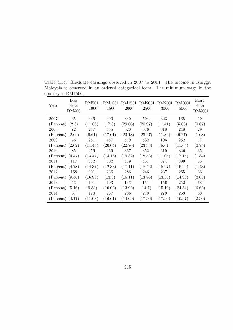
Table 4.14: Graduate earnings observed in 2007 to 2014. The income in RinggitMalaysia is observed in an ordered categorical form. The minimum wage in thecountry is RM1500.
YearLessthan
RM500
RM501- 1000
RM1001- 1500
RM1501- 2000
RM2001- 2500
RM2501- 3000
RM3001- 5000
Morethan
RM5001
2007 65 336 490 840 594 323 165 19(Percent) (2.3) (11.86) (17.3) (29.66) (20.97) (11.41) (5.83) (0.67)2008 72 257 455 620 676 318 248 29(Percent) (2.69) (9.61) (17.01) (23.18) (25.27) (11.89) (9.27) (1.08)2009 46 261 457 519 532 196 252 17(Percent) (2.02) (11.45) (20.04) (22.76) (23.33) (8.6) (11.05) (0.75)2010 85 256 269 367 352 210 326 35(Percent) (4.47) (13.47) (14.16) (19.32) (18.53) (11.05) (17.16) (1.84)2011 117 352 302 419 451 374 399 35(Percent) (4.78) (14.37) (12.33) (17.11) (18.42) (15.27) (16.29) (1.43)2012 168 301 236 286 246 237 265 36(Percent) (9.46) (16.96) (13.3) (16.11) (13.86) (13.35) (14.93) (2.03)2013 53 101 103 143 151 156 252 68(Percent) (5.16) (9.83) (10.03) (13.92) (14.7) (15.19) (24.54) (6.62)2014 67 178 267 236 279 279 263 38(Percent) (4.17) (11.08) (16.61) (14.69) (17.36) (17.36) (16.37) (2.36)
215

a total number of 686 cohorts, with some cohorts are not observed. For example
there are no Chinese studying Islamic studies which reduces our cohort observation
by 16. Cohort occurrences is summarised in Table 4.16. 70% of the cohorts occur
for all eight years of our observations. The dependent variable is graduate income
in an ordered form. We would model the earning as if we are observing genuine
panel. Table 4.17 shows the mean of graduate income (ranges between 1 to 8)
across different course of study and year.
216

Table 4.15: Definition and measurement of variables.
Variable Cohort averaging process Measurement
gradinc Cohort means of income. Observed in eight categories withthe lowest (<RM500) and thehighest category (>RM5,000).
cgpa Cohort means of CGPA. Cumulative grade point average(CGPA) to measure academicperformance.
muet Cohort means of MUETscore.
Six bands of MUET score, thelowest Band 1 to the highestBand 6 indicating proficiency inusing English in writing,listening, and speaking.
faminc Cohort mean of familyincome.
Observed in eight categories withthe lowest (<RM500) and thehighest category (>RM5,000).
age Cohort mean age.
urban Proportion of cohorts livingin urban states.
Urban states include KlangValley and Penang.
joburban Proportion of cohortsworking in urban states.
Urban states include KlangValley and Penang.
public Proportion of cohortsworking in the publicsector.
permanent Proportion of cohortsworking as permanent.
professional Proportion of cohortsworking as professional.
year Years fo when the survey isconducted or when thecohorts graduated.
217
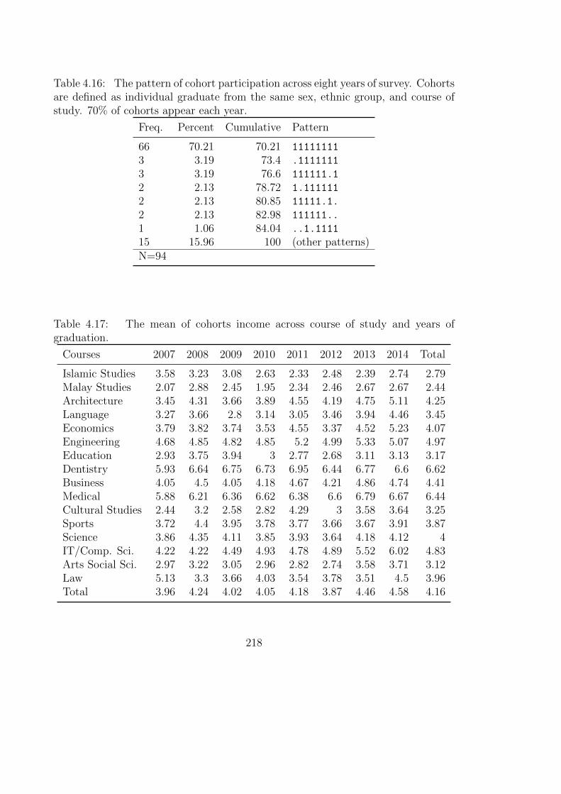
Table 4.16: The pattern of cohort participation across eight years of survey. Cohortsare defined as individual graduate from the same sex, ethnic group, and course ofstudy. 70% of cohorts appear each year.
Freq. Percent Cumulative Pattern
66 70.21 70.21 11111111
3 3.19 73.4 .1111111
3 3.19 76.6 111111.1
2 2.13 78.72 1.111111
2 2.13 80.85 11111.1.
2 2.13 82.98 111111..
1 1.06 84.04 ..1.1111
15 15.96 100 (other patterns)N=94
Table 4.17: The mean of cohorts income across course of study and years ofgraduation.
Courses 2007 2008 2009 2010 2011 2012 2013 2014 Total
Islamic Studies 3.58 3.23 3.08 2.63 2.33 2.48 2.39 2.74 2.79Malay Studies 2.07 2.88 2.45 1.95 2.34 2.46 2.67 2.67 2.44Architecture 3.45 4.31 3.66 3.89 4.55 4.19 4.75 5.11 4.25Language 3.27 3.66 2.8 3.14 3.05 3.46 3.94 4.46 3.45Economics 3.79 3.82 3.74 3.53 4.55 3.37 4.52 5.23 4.07Engineering 4.68 4.85 4.82 4.85 5.2 4.99 5.33 5.07 4.97Education 2.93 3.75 3.94 3 2.77 2.68 3.11 3.13 3.17Dentistry 5.93 6.64 6.75 6.73 6.95 6.44 6.77 6.6 6.62Business 4.05 4.5 4.05 4.18 4.67 4.21 4.86 4.74 4.41Medical 5.88 6.21 6.36 6.62 6.38 6.6 6.79 6.67 6.44Cultural Studies 2.44 3.2 2.58 2.82 4.29 3 3.58 3.64 3.25Sports 3.72 4.4 3.95 3.78 3.77 3.66 3.67 3.91 3.87Science 3.86 4.35 4.11 3.85 3.93 3.64 4.18 4.12 4IT/Comp. Sci. 4.22 4.22 4.49 4.93 4.78 4.89 5.52 6.02 4.83Arts Social Sci. 2.97 3.22 3.05 2.96 2.82 2.74 3.58 3.71 3.12Law 5.13 3.3 3.66 4.03 3.54 3.78 3.51 4.5 3.96Total 3.96 4.24 4.02 4.05 4.18 3.87 4.46 4.58 4.16
218

4.4.1 Fixed effects ordered logit model of graduates earn-
ings.
The main purpose of this section is to look at the possibility of tracking cohorts
and model them as genuine panel. Estimation by pooled ordered model suffers from
unobserved cohort heterogeneity. Another alternative is to use Mundlak’s correlated
random effect approach but this method requires a strong assumption on the time
invariant unobserved component (see Wooldridge (2010) Ch 16 pp. 662). Instead,
we use the new proposed estimator by modelling cohort earning using a fixed effects
ordered logit model (FEOL). There are several estimators being introduced in the
literature, in this paper we focus on two estimators which will be described later.
Using FEOL, we can obtain the treatment effect of other variables while controlling
for stable characteristics of cohorts. We know for example that Chinese, male and
graduates from certain courses tend to earn higher wage, now that we can control
for the cohort effect (gender, ethnic, course of study) we can estimate the effect of
academic performance, English competency, and other job characteristics on cohort
incomes. By using fixed effects model we can also control for more difficult variables
such as intelligence, upbringing, and heredity that coincide with cohort effects that
might also influence earnings. FEOL allows these unobserved variables to have
correlation with the observed variables (Allison, 2009).
The drawback of fixed effects model is that it cannot estimate the time-invariant
variables. Furthermore, if the differences within individual is small, while the dif-
ferences between individual is great, then fixed effects model may give imprecise
estimates. From computational aspect, the development of fixed effects estima-
tion for ordered variable is ongoing and there is no standard package available for
analysis. While there is no available program to run FEOL, there are developing
219

literatures on finding estimators that is efficient. Efficient estimators such as blow-
up and cluster (BUC) (Baetschmann et al., 2015), Das van Soest (DvS) (Das and
Van Soest, 1999), and conditional likelihood estimator (CLE) (Muris, 2016) will be
discussed in the following.
For each cohort i observed in time t, the earning is given in ordered scale y∗it, which
is related to a latent variables yit as
y∗it = k if µk < yit ≤ µk+1 and k = 1, . . . , K. (4.15)
where µ are unknown parameters to be estimated with β, and are strictly increasing
(µk < µk+1 ∀k). The error term εit ∼ IID and standard logistic. The probability of
observing the outcome k for cohort i at time t is
Pr(y∗it = k|Xit, αi) = Λ(µk+1 −Xitβ − αi)− Λ(µk −Xitβ − αi) (4.16)
where Λ(X) = exp(X)/(1 + exp(X)) is CDF of the logistic distribution and we set
µ0 = −∞ and µK =∞. The MLE is affected by the incidental parameter problem
since the number of parameter in the likelihood function grows with the sample size
n. The estimator β based on this will be inconsistent for n → ∞ if T is fixed.
However in this case we have T = 8 hence the incidental parameter problem is
minimised.
For the binary choice panel data model, Chamberlain (1980) suggested an approach
based upon a conditional likelihood, conditioning on sufficient statistics for the nui-
sance parameters ai. Then the minimum sufficient statistics for ai is yit. It does not
depend on the incidental parameter ai and the conditional MLE of β is, under mild
regularity conditions, consistent and asymptotically normal. However, this approach
220
cannot be directly extended to an ordered panel data model where the dependent
variables has p > 2 possible outcomes.
As a solution, Winkelmann and Winkelmann (1998) suggested to collapse y∗it to
binary. The ordered dependent variable is dichotomised at cutoff k : dkit = 1(y∗it ≥
k)9. Next, we use Chamberlain’s estimator for fixed effects binary logit model.
Chamberlain’s binary logit fixed effect estimator uses the fact that conditioning the
individual likelihood contribution on the sum of the outcome over time provides
an expression which is independent of the fixed effects. The effect of time-varying
regressors can be estimated by conditional maximum likelihood.
Chamberlain show that maximising the conditional log-likelihood gives consistent
estimate of β. If the estimator β at each cutoff is consistent, we can estimate for
all each possible K − 1 cutoffs. Then, we can combine the estimation results by
minimum distance estimation, taking into account the weight given by the inverse
of their variance. The solution is proposed by Das and Van Soest (1999) and is
called DvS estimator. However, if there is only a small overlap between sample
contributing to the conditional maximum likelihood logit estimator, then the small
sample problem may lead to convergence problem.
To overcome this, Baetschmann et al. (2015) proposes estimating all dichotomisation
jointly subject to the restriction βk = β ∀k = 2, . . . , K. The proposed estimator
called the Blow-up and Cluster (BUC) - first generate data set where each individual
is repeated K − 1 times (blowing up the sample size). Then dichotomise every
K−1 copies of individual at different cutoff points. Next, estimate using conditional
maximum likelihood using the entire sample. The standard error should be adjusted
for clustering (by using sandwich variance estimator) as some individual contribute
9But any particular choice of cutoff leads to some observation been discarded because individualwith constant dkit do not contribute to the likelihood function.
221

to several terms in the log-likelihood function. Unlike DvS, BUC do not suffer from
small sample size problems.
However, the existing estimators (i.e. DvS, BUC) do not estimate the cut point
differences. For this reason, the model cannot compute the partial effects of ex-
planatory variables hence prevent the examination of the magnitude of regression
coefficients. The model’s inability to compute marginal effect hamper its usability
in the empirical applications (Muris, 2016). In light of this, Muris (2016) proposed
a new estimator that can simultaneously estimate the cut point differences and use
the information to bound a marginal effect.
Muris (2016) proposed to convert an ordered logit model with J outcomes, T ob-
servations into binary choice logit in (J − 1)T ways before applying Chamberlain’s
conditional MLE to each binary choice model. The ordered variable is transformed
into binary by yit ≤ π(t) for any time series of cutoff categories π(t), t = 1, . . . , T .
The resulting binary time series after applying transformation π = (π(t))Tt=1 is
di,π = (di,t,π = 1{yit ≤ π(t)}, t = 1, . . . , T ) or di,t,π = 1[αi + Xitβ + uit < µπ(t)].
The additional information that we obtained from the cut point differences can
inform us of how far apart the categories are (Muris, 2016).
4.4.2 FEOL result.
The preceding part discusses the estimation results of two chosen fixed effects or-
dered logit models - the BUC and the CLE. We investigate the relationship between
cohort’s academic achievement, English language ability, cohort’s characteristics and
their job attributes. To date, there have been no studies done on graduates cohort
earning due to the data limitation and this analysis is the first to examine this phe-
nomenon. We take cohort average from 28,666 individuals to create theoretically 96
222
cohorts that appear at least once in the 8 years period. A total number of cohort ×
year is 686 will be used in the analysis. Cohort’s income is observed in an ordered
category similar to individual earning that we have consistently used in the previous
chapters.
A precaution in using cohorts is that it is not a genuine panel. For a genuine panel,
we observe the same individual graduates from the first year they finished study
and we observe their career progression for at least several years in which we would
expect that they would increase their earnings by either moving into better occupa-
tional category, or among those who are unemployed we would expect them to end
their unemployment period. However, careful interpretation should be taken when
analysis is done on cohorts because each year we are still observing cohort character-
istics in their first year after finishing study. Any changes in their earning reflect the
changes of graduate’s other time-changing variables such as academic achievement,
English language ability, family income, age, location, and job attributes. Between
cohorts with the same sex and race, and took the same course, any changes in the
time-changing variables would affect their earning. A significant coefficient in any
of the included variables signifies the impact of such variable towards changes in
earning.
Controlling for cohort heterogeneity, we found that the effect of academic achieve-
ment and English language ability disappear and becoming insignificant in the FEOL
model. Indeed, only family income and locality remain significant - higher family
income and originating from an urban state increase graduates’ earning. Our result
is consistent with Chapman and Harding (1985) who found that intergenerational
inheritance and residential location play a very important role in Malaysia. Our
finding shows that the situation still occurs among those who have invested in ed-
ucation which is suppose to moderate the effect of intergenerational inheritance.
223

Among all the job characteristics included in the model, only permanent position is
significantly associated with higher graduate earning.
The results show that among graduates of the same sex and race and took the same
courses of study, only family income and locality play important roles in changes of
earning surpassing the other cohort characteristics. Family income and residing in
an urban area are also related to each other, since families who live in the urban
areas generally earn higher than those from the rural.
Nevertheless, the interpretation of the result must be taken with caution. First,
we only observe a group of individuals who share the same fixed membership where
these individuals are correlated to each other. Yet, they are not identical. We would
recommend to collect data on the same individual for several years. From here, we
can actually see the trend in the earning of the same individuals that may help to
gain better understanding on graduates career mobility after several years leaving
their education. With the current data we only observe graduates’ employment and
earning within a very short time frame which may not provide complete picture of
graduate employment since there are graduates who are still embarking on successive
education, took a transitory jobs, or remain in the job search process - which limit
our understanding on the graduates careers as a whole.
224
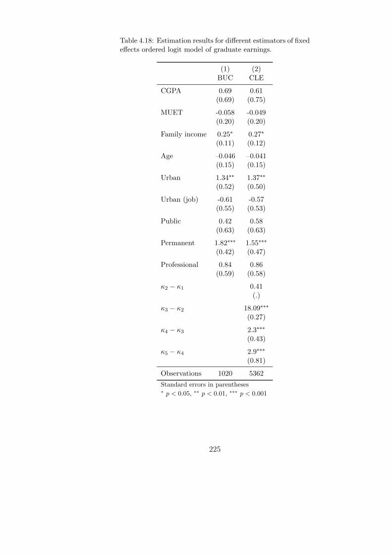
Table 4.18: Estimation results for different estimators of fixedeffects ordered logit model of graduate earnings.
(1) (2)BUC CLE
CGPA 0.69 0.61(0.69) (0.75)
MUET -0.058 -0.049(0.20) (0.20)
Family income 0.25∗ 0.27∗
(0.11) (0.12)
Age –0.046 –0.041(0.15) (0.15)
Urban 1.34∗∗ 1.37∗∗
(0.52) (0.50)
Urban (job) -0.61 -0.57(0.55) (0.53)
Public 0.42 0.58(0.63) (0.63)
Permanent 1.82∗∗∗ 1.55∗∗∗
(0.42) (0.47)
Professional 0.84 0.86(0.59) (0.58)
κ2 − κ1 0.41(.)
κ3 − κ2 18.09∗∗∗
(0.27)
κ4 − κ3 2.3∗∗∗
(0.43)
κ5 − κ4 2.9∗∗∗
(0.81)
Observations 1020 5362
Standard errors in parentheses∗ p < 0.05, ∗∗ p < 0.01, ∗∗∗ p < 0.001
225
4.5 Conclusion.
This chapter shed a light on several aspects that is under-explored in the litera-
ture of graduate employment, particularly in Malaysia. The first section dealt with
examining factors that lead to the decision to migrate and how those decision af-
fect employment outcomes such as education-job match and earning. By separating
the analysis based on four migration patterns we are able to see motivation behind
movement from and to an urban or non-urban states. Consistent with our assump-
tion, migration from non-urban to an urban state significantly increases earning. In
fact, all migrating graduates earn significantly more than non-migrating graduates.
However, the relationship between migration and education-job mismatch is more
mixed.
The second chapter analysed the time taken to obtain the first job using survival
analysis. The same attributes that are associated with better employment outcomes
do not necessarily lead to faster transition, indeed, higher CGPA and more attractive
courses correspond to longer transition on the basis that graduates prolong their job
search period if they think they can do better.
The third part looks at the possibility to track the cohort of graduates and observe
cohort’s earning over the years. While controlling for the unobserved heterogeneity
of cohort effects, we use fixed effects ordered logit model to estimate the impact of
several cohorts averaged variables towards their earning. The result shows that fam-
ily income and locality consistently contributes to the estimation of cohort earning.
226

4.6 Appendix.
(1)y=Employed
CGPA 0.137∗∗∗ (0.0178)Band 2 0.0206 (0.0237)Band 3 -0.00114 (0.0245)Band 4 -0.0368 (0.0287)Band 5 -0.0277 (0.0451)Band 6 0.0545 (0.159)Arts/SocSc -0.289∗∗∗ (0.0587)Transport 0.322∗∗ (0.115)Administration 0.202∗∗∗ (0.0584)Management 0.0133 (0.0558)Economy -0.0533 (0.0648)Accountancy 0.270∗∗∗ (0.0581)Marketing -0.112 (0.0662)Finance 0.0362 (0.0587)Journalism -0.0335 (0.0650)Islamic 0.0761 (0.0705)Food/hospitality 0.0402 (0.0668)Arts -0.209∗∗ (0.0637)Pure science -0.239∗∗∗ (0.0681)Applied science -0.217∗∗∗ (0.0568)Pharmacy -0.629∗∗∗ (0.0929)Medical 0.685∗∗∗ (0.0673)Dentistry -0.451∗∗∗ (0.128)Nurse -0.0533 (0.0696)Environment -0.0661 (0.0640)Sports -0.290∗∗ (0.0996)Engineering 0.0252 (0.0542)CompSci 0.173∗∗ (0.0574)Education -0.386∗∗∗ (0.0577)Male 0.0740∗∗∗ (0.0127)Age 0.0854∗∗∗ (0.00611)Malay -0.0313 (0.0195)Chinese 0.355∗∗∗ (0.0228)RM 501 - RM 1000 0.0749∗∗ (0.0237)RM 1001 - RM 1500 0.120∗∗∗ (0.0245)RM 1501 - RM 2000 0.170∗∗∗ (0.0257)RM 2001 - RM 2500 0.159∗∗∗ (0.0276)
227

RM 2501 - RM 3000 0.122∗∗∗ (0.0264)RM 3001 - RM 5000 0.0749∗∗ (0.0264)> RM 5000 0.0758∗ (0.0295)Married 0.914 (0.700)experience 0.272∗∗∗ (0.0121)Constant -2.882∗∗∗ (0.172)
Observations 50703
Standard errors in parentheses∗ p < 0.05, ∗∗ p < 0.01, ∗∗∗ p < 0.001
228
Chapter 5
Conclusion
5.1 Summary of results
This thesis studies several aspects related to graduates transition from education
to their first destinations after study. The first chapter confirms previous studies
related to graduate employment outcomes in which graduates with better academic
achievement, better English proficiency, took certain courses of study, and coming
from certain socio-economic background (i.e. older, Chinese, higher family income,
and originating from an urban state) generally have better occupational outcomes
such as being able to secure full time, professional, and permanent jobs. Further
analysis shows that gender differences exist between different sexes - men generally
have better employment outcomes than women, but men are also more likely to
take up more challenging courses which are associated with superior job categories.
Women have the tendency to choose less attractive courses which are associated with
low employment rate, more heterogenous occupational categories, and low income.
To some extent, this tendency may rationalise women’s under-representation in high
229
skilled jobs associated with high remuneration. Moreover, there is a paradoxical the-
ory stating that women intentionally prefer less demanding jobs to balance between
work and families.
However, the situation may be reasonable for the whole women population, but we
would expect the situation would be different in the case of women graduates who
have invested a huge sum of money, sacrifice their forgone earning, time and effort
to gain a qualification at the tertiary level of education. This progressive action
to improve productivity and investment in their human capital should translate
into women’s equal share in the labour force participation and equal earning with
men. Rationally after controlling for courses of study the effect of women should
disappear but we found persistent gender segregation within different occupation
types especially those in highly industrialised sectors.
We even investigated further the gender difference in gaining full time employment
among female graduates who have similar qualification as men and found that women
in Engineering, Computer Sciences, and Transport studies have lower employment
rate, all else equal. Due to the inter-connection between taking Engineering course
and working in the Manufacturing industry, both parts show that women are se-
riously under-represented and the differences are largely due to some unobserved
features which may be ascribed to discrimination or taste (women might prefer less
demanding jobs). Our result is consistent with another study among women workers
in the Manufacturing industry (Osman and Shahiri, 2014)(Osman-Rani, 1982).
Not only women are under-represented in the better occupational categories, the sec-
ond chapter shows that women are under-paid after controlling for SES, educational,
and job attributes. Women generally have higher CGPA but they took less attrac-
tive courses which hamper their wage determination. We found evidence of gender
gap where women earn significantly lower especially in the case of the private sector
230

(i.e. Manufacturing). Necessary actions need to be taken to devise a policy that will
reduce the imbalance participation rate by encouraging female labour force partic-
ipation in those industries. In the case of Malaysia, women have the same right as
men (same working hours, no employment ban) but women’s lower employment rate
in high skilled industries is perhaps due to restrictions such as the determination of
maternity leave, small children, avoiding dangerous jobs, and cultural expectation.
If that is the case, we need to reinforce policies to support women’s employment
such as the implementation of maternity and paternity leave (so that childcare is
distributed equally between parents), to promote for flexible working hours, and
the provision of childcare facilities at work. There should be a policy intervention
among women graduates who took Engineering course because if they perform as
good as men and having the same qualification, their under-representation in labour
force participation can be a huge waste of talent. Universities should then send the
right signal so that prospective students taking Engineering courses have complete
information of their employment prospects after graduation. The policy implication
of women enrolment into higher education by merit alone may just do more harm if
it encourages unnecessary investment in tertiary education for some women if there
is no action taken to rectify gender differences in employment opportunity.
Another major finding of this thesis is the persistence of ethnic imbalance in the
economy among Malaysian youth in which the Malays are under-represented in
better occupational categories and earn lower than the other ethnic groups. Malay’s
under-performance in securing better jobs is due to their choice of less attractive
courses, lower academic achievement, and come from families with low income and
low education. Malays are also more likely to be originated from non-urban states
with limited job availability which require Malay graduates to migrate, but migration
is costly. If the imbalance in the ethnic share persists while the intergenerational
inheritance is strong, the disparity will continue to deteriorate - Malays will remain in
231

the lower income trap and the Chinese will continue to be economically progressive.
The National Economic Policy which was introduced to eradicate poverty did not
achieve its intended goal. Due to poor implementation, the NEP does not show
improvement in social mobility among Malays except very few aristocrats; it rather
creating a serious intra-ethnic gap within the Malay community. Another critic for
the poor execution of NEP is ignoring the minority ethnic Indian who remain in
poverty (among those living in the estates). The intervention in the public univer-
sity quota does not efficiently remove the gap, partly because even though Malay’s
participation in tertiary education has increased but the admission is offered to less
attractive courses that have low market demand. The finding suggests that offering
certain types of courses that have low marketability may lead to skill wastage in
a sense that graduates spend their time and money for their study but they end
up with jobs that may not compensate for their educational investment. One way
to intervene this issue is to reduce the intake for less attractive courses that have
heterogenous marketability, instead, offer more STEM and vocational courses that
can be more practical in the labour market. The admission to courses that are less
profitable but have high social benefit should be reduced to cater for the need of
knowledge creation but not as an investment for human capital. Another aspect that
should be taken care of is the educational achievement among the rural Malays so
they can perform better and consequently able to take up more challenging courses
which lead to better jobs. Seeing education as the key to upgrade the socio-economic
status of an individual, more equally distributed resources for education should be
enhanced to includes the children of the disadvantages. Awareness of the importance
of education should be promoted among low-income families in the rural.
The third chapter covers a different aspect of graduate’s transition from education
to work. The analysis of migration shows that higher ability graduates are more
232

likely to migrate and their migration reflects in their higher earnings. There is
also some sort of correlation between attending selective universities in the urban
areas and high ability graduates because the top universities are located in the
urban states hence urban and non-urban graduates who attend urban institutions
are more likely to stay at the location of their education. We also found that
better job characteristics are associated with all migrating patterns, which only
strengthen our assumption that graduates choose to migrate to obtain better jobs
and to compensate for their higher ability (human capital).
An analysis on the transition time elapsed between finishing study and obtaining the
first job show that with the exception of SES variables, the determinants that lead
to better occupational categories and higher income are associated with a longer
instead of faster transition. Graduates with higher CGPA and took more attractive
courses are more likely to prolong their job search which results in attaining better
job characteristics. Older graduates with higher academic achievement and who
took more attractive courses associated with higher earning eventually have a longer
transition from education to work. The finding confirms the job search theory which
states that an individual with high ability may lengthen their job search period if
they think they can do better by not accepting the first job offer. We found that
graduates from all economic background find a job at the same rate, but graduates
from lower family income find jobs in the lower occupational category and generally
have lower income.
The final part of the thesis shows that for a cohort with similar sex and ethnic
group and took the same course, the change of their first job earning is attributable
to their family income, originating from an urban state, and holding a permanent
job. Family income and residing in an urban area are also related to each other
since families who live in the urban areas generally earn higher than those from the
233
rural. Intergenerational inheritance is found to be persistent even among graduates
who have obtained a high level of education in which family’s economic background
and locality still play a role in determining an individual’s earning hence education,
even at tertiary level, has not successfully moderated the effect of social immobility.
5.2 Limitation and future recommendation
This thesis leaves open important avenues for future research. First, parent edu-
cation is probably more relevant than parent income because children with higher
parent education tend to have upward mobility than those with lower parent edu-
cation (i.e. upbringing, connection, genetic heredity). A graduate that comes from
lower parent education is the first generation of university student so they are sur-
viving in the professional world without guidance from their parents. Second, if
the income is observed in an interval form then more analysis can be done such as
the quantile regression analysis to examine the effect of the variance in the wage
decomposition. Third, women’s and Malay’s preference for certain type of courses
and jobs could be an interesting subject to study that may explain their inferior
performance in their employment outcomes hence school performance would help
to understand their choice of courses of study. Fourth, if a graduate’s earning can
be observed for several years after graduation then we can study the effect of part
time jobs in graduate’s subsequent earning whether the part time job is transitory
or have a permanent effect on graduate’s career.
234
Bibliography
Abdullah, K., Noor, N. M., & Wok, S. (2008). The perceptions of women’s roles and
progress: A study of Malay women. Social indicators research, 89(3), 439-455.
Adamchik, V. (1999). The Effect of Unemployment Benefits on the Probability of
Re-employment in Poland. Oxford Bulletin of Economics and Statistics, 61(1),
95-108.
Albrecht, J., Bjorklund, A., & Vroman, S. (2003). Is there a glass ceiling in Sweden?.
Journal of Labor economics, 21(1), 145-177.
Allison, P. D. (2009). Fixed effects regression models (Vol. 160). SAGE publications.
Altonji, J. G. & Blank, R. M. (1999). Race and Gender in the Labor Market. Hand-
book of Labor Economics. Vol. 3, Chapter 48, pp. 3144-3213.
Arrow, K. J. (1973). Higher education as a filter. Journal of public economics, 2(3),
193-216.
Amemiya, T. (1981). Qualitative response models: A survey. Journal of economic
literature, 19(4), 1483-1536.
Angrist, J. D., & Pischke, J. S. (2008). Mostly harmless econometrics: An empiri-
cist’s companion. Princeton university press.
235

Arulampalam, W., Booth, A. L., & Bryan, M. L. (2007). Is there a glass ceiling over
Europe? Exploring the gender pay gap across the wage distribution. Industrial &
Labor Relations Review, 60(2), 163-186.
Assaad, R., Krafft, C., & Salehi-Isfahani, D. (2014). Does the type of higher education
affect labor market outcomes? A comparison of Egypt and Jordan. In Economic
Research Forum Working Paper Series No (Vol. 826).
Azam, M., Chin, A., & Prakash, N. (2013). The returns to English-language skills
in India. Economic Development and Cultural Change, 61(2), 335-367.
Baetschmann, G., Staub, K. E., & Winkelmann, R. (2015). Consistent estimation
of the fixed effects ordered logit model. Journal of the Royal Statistical Society:
Series A (Statistics in Society), 178(3), 685-703.
Bauer, T. K., & Sinning, M. (2006). An Extension of the Blinder- Oaxaca Decom-
position to Non-Linear Models, RWI Discussion Papers, No. 49.
Becker, Gary S., (1971). The Economics of Discrimination,University of Chicago
Press Economics Books, University of Chicago Press, edition 2.
Becker, G. S. (1975). Front matter, human capital: a theoretical and empirical anal-
ysis, with special reference to education. In Human Capital: A Theoretical and
Empirical Analysis, with Special Reference to Education, Second Edition(pp. 22-
0). NBER
Becker, G. S. (1985). Human capital, effort, and the sexual division of labor. Journal
of Labor Economics, 3(1), S33-S58.
Bellante, D. and Link, A.N. (1981), Are public sector workers more risk averse than
private sector workers?, Industrial and Labor Relations Review 34(3), 408-412.
236
Bender, K. A. and R. F. Elliot (1999), Relative earnings in the UK public sector:
the impact of pay reform on pay structure?, in R. Elliot, C. Lucifora and D.
Meurs (eds.), Public sector pay determination in the European Union, London:
McMillan Press Ltd., pp. 285-339.
Bender, K. A. (1998). The central government private sector wage differential. Jour-
nal of Economic Surveys, 12(2), 177-220.
Bender, K. A. (2003), Examining Equality Between Public and Private Sector Wage
Distributions, Economic Enquiry, Vol. 41, No. 1, pp. 62-79.
Bender, K. A., Donohue, S. M., & Heywood, J. S. (2005). Job satisfaction and
gender segregation. Oxford economic papers, 57(3), 479-496.
Biggeri, L., Bini, M., & Grilli, L. (2001). The transition from university to work: a
multilevel approach to the analysis of the time to obtain the first job. Journal of
the Royal Statistical Society: Series A (Statistics in Society), 164(2), 293-305.
Blau, F. D., & Kahn, L. M. (2000). Gender differences in pay National bureau of
economic research.
Blinder, A. S. (1973). Wage discrimination: reduced form and structural estimates.
Journal of Human resources, 436-455.
Borjas, G. J. (1980). Wage determination in the federal government: The role of
constituents and bureaucrats. The Journal of Political Economy, 1110-1147.
Borland, J., Gregory, R. G., & Sheehan, P. (2001). Work rich, work poor: inequality
and economic change in Australia.
Brown, C. & Corcoran, M. (1997). Sex-Based Differences In School Content And
The Male/Female Wage Gap, Journal of Labor Economics, v15(3,Jul), Part 1,
431-465.
237
Buchel, F., & Mertens, A. (2004). Overeducation, undereducation, and the theory of
career mobility. Applied Economics, 36(8), 803-816.
Buchel, F., & Van Ham, M. (2003). Overeducation, regional labor markets, and
spatial flexibility. Journal of Urban Economics, 53(3), 482-493.
Cain, G. G. (1986). The economic analysis of labor market discrimination: a survey.
in Handbook of Labor Economics, by Ashenfelter, O & Card, D. Elsevier Science.
Chamberlain, G. (1979). Analysis of covariance with qualitative data, Review of
Economic Studies, 47, pp. 225-238.
Chapman, B. J., & Harding, J. R. (1985). Sex differences in earnings: An analysis
of Malaysian wage data. Journal of Development Studies, 21(3), 362-376.
Cheng, S., & Long, J. S. (2007). Testing for IIA in the multinomial logit model.
Sociological methods & research, 35(4), 583-600.
Chevalier, A. (2011). Subject choice and earnings of UK graduates. Economics of
Education Review, 30(6), 1187-1201.
Ciriaci, D. (2014). Does university quality influence the interregional mobility of
students and graduates? The case of Italy. Regional Studies, 48(10), 1592-1608.
Colella, F. (2014). Women’s Part-Time/Full-Time Wage Differentials in Europe:
An Endogenous Switching Model.
Das, M., & Van Soest, A. (1999). A panel data model for subjective information on
household income growth. Journal of Economic Behavior & Organization, 40(4),
409-426.
Daymont, T. N. and Andrisani, P. J. (1984), Job Preferences, College Major, and
the Gender Gap in Earnings, Journal of Human Resources, pp. 408-428.
238
Deaton, A. (1985). Panel data from time series of cross-sections. Journal of econo-
metrics, 30(1), 109-126.
Dekker, R., De Grip, A., & Heijke, H. (2002). The effects of training and overedu-
cation on career mobility in a segmented labour market. International Journal of
Manpower, 23(2), 106-125.
Malaysian Department of Statistics: Population and Demography.
https://www.dosm.gov.my/v1/index.php?r=column/ ctwoByCat&parent id=115
&menu id= L0pheU43NWJwRWVSZklWdzQ4TlhUUT09 (Accessed on
27/2/2017).
Devadason, E. S., Subramaniam, T., & Daniel, E. G. S. (2010). Final year under-
graduates? perceptions of the integration of soft skills in the formal curriculum:
a survey of Malaysian public universities. Asia Pacific Education Review, 11(3),
321-348.
Disney, R., and Gosling, A. (2008), Changing public sector wage differentials in the
UK, (No. 08/02). IFS Working Papers, Institute for Fiscal Studies.
Dolton, P. J., Makepeace, G. H., & van der Klaauw, W. (1989). Occupational choice
and earnings determination: The role of sample selection and non-pecuniary fac-
tors. Oxford Economic Papers, 41(3), 573-594.
Drydakis, N. (2016). The effect of university attended on graduates’ labour market
prospects: A field study of Great Britain. Economics of Education Review, 52,
192-208.
Duncan, G. J., & Hoffman, S. D. (1981). The incidence and wage effects of overed-
ucation. Economics of Education Review, 1(1), 75-86.
239
Elliott, R. F., & Duffus, K. (1996). What Has Been Happening to Pay in the Public
Service Sector of the British Economy? Developments over the Period 1970-1992.
British Journal of Industrial Relations, 34(1), 51-85.
England, P., Allison, P., & Wu, Y. (2007). Does bad pay cause occupations to fem-
inize, does feminization reduce pay, and how can we tell with longitudinal data?
Social Science Research, 36(3), 1237-1256.
Faggian, A., & McCann, P. (2009). Human capital, graduate migration and innova-
tion in British regions. Cambridge Journal of Economics, 33(2), 317-333.
Fairlie, R. W. (1999). The absence of the African-American owned business: An
analysis of the dynamics of self-employment. Journal of Labor Economics, 17(1),
80-108.
Fairlie, R. W. (2005). An extension of the Blinder-Oaxaca decomposition technique
to logit and probit models. Journal of economic and social measurement, 30(4),
305-316.
Fallon, P., & Verry, D. (1988). The economics of labour markets. Philip Allan Pub-
lishers, Oxford.
Figueiredo, H., Rocha, V., Biscaia, R., & Teixeira, P. (2015). Gender pay gaps
and the restructuring of graduate labour markets in Southern Europe. Cambridge
Journal of Economics, bev008.
Fogel, W., & Lewin, D. (1974). Wage determination in the public sector. Industrial
and Labor Relations Review, 410-431.
Glass, J. (1990). The impact of occupational segregation on working conditions. So-
cial Forces, 779-796.
240

Gomez, E.T. and Jomo, K.S. (1999) Malaysia’s Political Economy: Politics, Pa-
tronage and Profits, Cambridge: Cambridge University Press.
Greene, W. H. (2000). Econometric analysis, 4th ed. International edition, New
Jersey: Prentice Hall.
Green, F., & Zanchi, L. (1997). Trends in the training of male and female workers
in the United Kingdom. British Journal of Industrial Relations, 35(4), 635-644.
Gregory, R.G. and Borland, J. (1999), Recent developments in public sector labor
markets?, Handbook of Labor Economics 3, 3573-3630.
Griliches, Z. (1977). Education, Income, and Ability: Rejoinder to Cardell and Hop-
kins. Journal of Political Economy, 85(1).
Gunderson, M. (1980). Probit and logit estimates of labor force participation. Indus-
trial Relations: A Journal of Economy and Society, 19(2), 216-220.
Hanapi, Z., Nordin, M. S., & Khamis, A. (2015). Challenges faced by engineering
lecturers in integrating technical and employability skills in the curriculum: A case
study in Community College, Malaysia. International Journal of Social Science
and Humanity, 5(5), 483.
Hartog, J., Van Praag, M., & Van Der Sluis, J. (2010). If you are so smart, why
aren’t you an entrepreneur? Returns to cognitive and social ability: Entrepreneurs
versus employees. Journal of Economics & Management Strategy, 19(4), 947-989.
Hausman, J., & McFadden, D. (1984). Specification tests for the multinomial logit
model. Econometrica: Journal of the Econometric Society, 1219-1240.
Heckman, J. J. (1979), Sample Selection Bias for a Specification Error, Economet-
rica, Vol. 47, No. 1, pp 153-161.
241

Heitmueller, A. (2004), Public-Private Sector Wage Differentials in Scotland: An
Endogenous Switching Model, IZA Discussion Paper No. 992.
Hicks, J. (1963). The theory of wages. Springer.
Hilmer, M. J., & Hilmer, C. E. (2012). On the relationship between student tastes
and motivations, higher education decisions, and annual earnings. Economics of
Education Review, 31(1), 66-75.
Hirschman, C. 1983. Labor markets and ethnic inequality in Peninsular Malaysia.
Journal of Developing Areas 18: 1-20.
Iammarino, S., & Marinelli, E. (2015). Education-Job (Mis) Match and Interregional
Migration: Italian University Graduates’ Transition to Work. Regional Studies,
49(5), 866-882.
Ismail, N. A. (2011). Graduates’ characteristics and unemployment: A study among
Malaysian graduates. International journal of business and social science, 2(16).
James, E., Nabeel, A., Conaty, J., & To, D. (1989). College quality and future earn-
ings: where should you send your child to college? American Economic Review,
79, 247-252.
Jomo, K. S. (2004). The new economic policy and interethnic relations in Malaysia
identities, conflict and cohesion (Vol. 7). Geneva, Switzerland: United Nations
Research Institute for Social Development.
Kanapathy, V. (2006). Migrant workers in Malaysia: an overview.
In Country paper prepared for Workshop on East Asian Coopera-
tion Framework for Migrant Labour, Kuala Lumpur. Retrieved from
http://www.cpiasia.net/v3/images/policy papers/Migrant%20Workers
%20in%20Malaysia An%20Overview.pdf. (Accessed 21/2/2017).
242

Katz, L. F., & Krueger, A. B. (1992). The effect of the minimum wage on the
fast-food industry. Industrial & Labor Relations Review, 46(1), 6-21.
Koshy, P., Seymour, R., & Dockery, M. (2016). Are there institutional differences in
the earnings of Australian higher education graduates?. Economic Analysis and
Policy, 51, 1-11.
Jurajda, S., & Paligorova, T. (2006). Female managers and their wages in Central
Europe.
Lee, K. H., & Nagaraj, S. (1995). Male-female earnings differentials in Malaysia.
Journal of Development Studies, 31(2), 467-480.
Muller, W., & Gangl, M. (2003). The transition from school to work: a European
perspective. Transitions from education to work in Europe. The integration of
youth into EU labour markets, 1-22.
Maddala, G. S. (1986). Limited-dependent and Qualitative Variables in Econometrics
No. 3, Cambridge university press.
Madden, D. (2010). Gender differences in mental well-being: a decomposition anal-
ysis. Social indicators research, 99(1), 101-114.
Makepeace, G. & Pal, S., 2004. Understanding the Effects of Sibling Composition
on Child, Labor and Demography 0402004, EconWPA.
Mata, J. & Machado, J. A. F., Counterfactual decomposition of changes in wage dis-
tributions using quantile regression. Journal of Applied Econometrics, 20(4):445-
465, 2005.
Mazumdar, D. (1981). The urban labor market and income distribution: A study of
Malaysia. A World Bank Research Publication.
243

McDaniel, A. (2012). Women’s advantage in higher education: towards understand-
ing a global phenomenon, Sociology Compass, vol. 6, 581-95
Melly, B., Decomposition of differences in distribution using quantile regression.
Labour Economics, 12(4):577-590, August 2005.
Migration Survey (2011), Malaysian Department of Statistics. Retrieved
from https://www.dosm.gov.my/v1/images/stories/files/LatestReleases/findings/
Summary findings Migras2011.pdf (Accessed on 25/2/2017).
Molho, I. (1987). The migration decisions of young men in Great Britain. Applied
Economics, 19(2), 221-243.
Moore, W. J., & Raisian, J. (1981). A time series analysis of the growth and deter-
minants of union/nonunion relative wage effects, 1967-1977 (Vol. 115). US Dept.
of Labor, Bureau of Labor Statistics, Office of Research and Evaluation.
Muris, C. (2016). Estimation in the fixed effects ordered logit model. Review of Eco-
nomics and Statistics.
Nagaraj, S. (2014). Gender imbalance in educational attainment and labour market
dynamics: Evidence from Malaysia. Malaysian Journal of Economic Studies, 51,
127.
Nakosteen, R. A., & Zimmer, M. (1980). Migration and income: the question of
self-selection. Southern Economic Journal, 840-851.
Nasrudin, M. (2004). Graduate Unemployment; Perspectives & Brief Analysis. Jour-
nal of Administrative Science.
Ng, C. W., & Chakrabarty, A. S. (2005). Women managers in Hong Kong: Personal
and political agendas. Asia Pacific Business Review, 11(2), 163-178.
244

Oaxaca, R. (1973), Male-female Wage Differentials in Urban Labor Markets, Inter-
national economic review, pp. 693-709.
Ong, E. (2012). Education and Labor Market Outcomes of Malaysia’s Affirmative
Action Policies.
Osman, Z., & Shahiri, H. (2014). Ethnic and gender inequality in employment during
the new economic policy. Institutions and Economics, 6(1), 57-72.
Osman-Rani, H. (1982) Manufacturing Industries, in E. K. Fisk and Osman- Rani,
H. (ed.) The Political Economy of Malaysia, Kuala Lumpur: Oxford.
Pillai, S., Khan, M. H., Ibrahim, I. S., & Raphael, S. (2012). Enhancing employability
through industrial training in the Malaysian context. Higher Education, 63(2),
187-204.
Polachek, S. (1976) Occupational Segregation: An Alternative Hypothesis, Journal
of Contemporary Business 5:1-12.
Polavieja, J. G. (2006). The incidence of temporary employment in advanced
economies: why is Spain different?. European Sociological Review, 22(1), 61-78.
Purcell, K., & Pitcher, J. (1996). Great Expectations: the new diversity of graduate
skills and aspirations. CSU.
Quinn, M. A., & Rubb, S. (2005). The importance of education-occupation matching
in migration decisions. Demography, 42(1), 153-167.
Rahmah et, al (2011). Employer Perceptions on Graduates in Malaysian Services
Sector. Medwell Journals, 5(3):184-193.
245
Rees, H., and Shah, A. (2000), An empirical analysis of self-employment in the UK,
Small Business: Critical Perspectives on Business and Management, Vol. 4, Issue
1, pp. 1414.
Reimers, C. W. (1983). Labor market discrimination against Hispanic and black
men. Review of Economics and Statistics 65: 570-579.
Rethinasamy, S., & Chuah, K. M. (2011). The Malaysian University English Test
(MUET) and its Use for Placement Purposes: A Predictive Validity Study. Elec-
tronic Journal of Foreign Language Teaching, 8(2), 234-245.
Robst, J., & VanGilder, J. (2016). Salary and job satisfaction among economics and
business graduates: The effect of match between degree field and job. International
Review of Economics Education, 21, 30-40.
Rosen, S. (1972). Learning and experience in the labor market. Journal of Human
Resources, 326-342.
Rosen, S. (1986). The theory of equalizing differences. in Handbook of Labor Eco-
nomics, by Ashenfelter, O & Card, D. Elsevier Science.
Rumberger, R. W. (1981). The rising incidence of overeducation in the US labor
market. Economics of Education Review, 1(3), 293-314.
Salas-Velasco, M. (2007). The transition from higher education to employment in
Europe: the analysis of the time to obtain the first job. Higher Education, 54(3),
333-360.
Salih, K., & Young, M. L. (1989). Changing conditions of labour in the semiconductor
industry in Malaysia. Labour and Society, 14(1989), 59-80.
Second Malaysia Plan. Retrieved from http://www.epu.gov.my/en/second-malaysia-
plan-1971-1975. (Accessed on 21/2/2017).
246

Selvaratnam, S. (1988). Population and status of women. Asia-Pacific Population
Journal, 3(2), 3-23.
Seshan, G. K., (2013). Public-Private-Sector Employment Decisions and Wage Dif-
ferentials in Peninsular Malaysia, Emerging Markets Finance and Trade, M.E.
Sharpe, vol. 49(S5), pages 163-179, November
Shahiri, H. (2012). An Analysis of the Reduction of the Ethnic Economic Gap in
Malaysia under the New Economy Policy: Evidence from Ethnic Occupation Seg-
regation and Wage Differential. Jurnal Ekonomi Malaysia, 46(2), 127-139.
Sicherman, N. (1991). “Overeducation” in the Labor Market. Journal of labor Eco-
nomics, 9(2), 101-122.
Sinning, M., Hahn, M., and Bauer, T. K. (2008), The Blinder-Oaxaca Decomposition
for Nonlinear Regression Models, The Stata Journal, Vol. 8, No. 4, pp. 480-492.
Sinning, M., Hahn, M., & Bauer, T. K. (2008). The Blinder-Oaxaca decomposition
for nonlinear regression models. The Stata Journal, 8(4), 480-492.
Sjaastad, L. A. (1970). The costs and returns of human migration. In Regional
Economics (pp. 115-133). Palgrave Macmillan UK.
Sloane, P. J. (2003) Much ado about nothing? What does the over-education litera-
ture really tell us?, in Buchel F., Degrip A. and Mertens A. (Eds) Overeducation
in Europe: Current Issues in Theory and Policy, pp. 11-48. Edward Elgar, Chel-
tenham.
Small, K. A., & Hsiao, C. (1985). Multinomial logit specification tests. International
economic review, 619-627.
247

Smith, J. P., Naylor, R. A., & McKnight, A. A. (2000). Graduate employment out-
comes and university performance measures. Economic Journal, 110(464), F382-
411.
Spence, M. (1973). Job market signaling. The quarterly journal of Economics, 87(3),
355-374.
Tam, T. (1997). Sex segregation and occupational gender inequality in the united
states: devaluation or specialized training? American Journal of Sociology, 102(6),
1652- 1692.
Tansel, A. 2005. Public-Private Employment Choice, Wage Differentials, and Gen-
der in Turkey. Economic Development and Cultural Change 53, no. 2: 453-477.
Teichler, U. (2000). Graduate employment and work in selected European countries.
European Journal of Education, 35(2), 141-156.
Terrell, K. (1993). Public-private wage differentials in Haiti Do public servants earn
a rent?. Journal of Development Economics, 42(2), 293-314.
Thurow, L. C. (1975). Generating Inequality: The Distributional mechanisms of the
economy. National Technical Information Service.
Tunali, I. (1986). A general structure for models of double-selection and an appli-
cation to a joint migration/earnings process with remigration. Research in labor
Economics, 8(Part B), 235-282.
Tunali, I. (2000). Rationality of migration. International Economic Review, 41(4),
893-920.
UNESCO (2012), Graduate Employability in Asia, UNESCO Bangkok, Asia and
Pacific Regional Bureau for Education.
248

Venhorst, V., & Corvers, J. G. F. (2015). Entry into working life: Spatial mobil-
ity and the job match quality of higher-educated graduates. Maastricht University
School of Business and Economics, GSBE.
Walker, I., & Zhu, Y. (2001). The returns to education: Evidence from the Labour
Force Surveys..
Weichselbaumer, D., & Winter-Ebmer, R. (2005). A Meta-Analysis of the Interna-
tional Gender Wage Gap. Journal of Economic Surveys, 19(3), 479-511.
Wharton, A. S., & Baron, J. N. (1987). So happy together? The impact of gender
segregation on men at work. American Sociological Review, 574-587.
Wilkinson, R., & Yussof, I. (2005). Public and private provision of higher education
in Malaysia: A comparative analysis. Higher Education, 50(3), 361-386.
Winkelmann, L., & Winkelmann, R. (1998). Why are the unemployed so unhappy?
Evidence from panel data. Economica, 65(257), 1-15.
Wooldridge, J. M. (2010). Econometric analysis of cross section and panel data.
MIT press.
World Bank (2011). Malaysia Economic Monitor - Brain Drain.
Washington, D.C.: The World Bank. April. Retrieved from
http://documents.worldbank.org/curated/en/282391468050059744/pdf/
614830WP0malay10Box358348B01PUBLIC1.pdf. (Accessed 21/2/2017).
The World Bank, World Urbanization Prospect (2015). Urban population.
Retrieved from http://data.worldbank.org/indicator/SP.URB.TOTL.IN.ZS (Ac-
cessed 21/2/2017).
Yavuzoglua, B., Tunali, I., & Ceyhanc, E. (2008). Correction of Selectivity Bias in
Models of Double Selection (Doctoral dissertation, Koc University).
249

Yun, M. S. (2004), Decomposing Differences in the First Moment. Economics letters,
Vol. 82, Issue 2, 275-280.
Zainudin, S. M. and Zulkifly, O. (1982) The Economic Structure, in E. K. Fisk
and Osman-Rani, H. (eds.), The Political Economy of Malaysia, Kuala Lumpur:
Oxford University Press.
Zanchi, L. (1998). Interindustry wage differentials in dummy variable models. Eco-
nomics Letters, 60(3), 297-301.
250