GPU Modeling of Ship Operations in Pack Ice · vessel performance in pack ice. The methodology is...
6
Paper No. ICETECH12-XYZ-R0 Daley Page number: 1 GPU Modeling of Ship Operations in Pack Ice Claude Daley Memorial University St. John's, Newfoundland and Labrador, Canada [email protected] Shadi Alawneh Memorial University St. John's, Newfoundland and Labrador, Canada Dennis Peters Memorial University St. John's, Newfoundland and Labrador, Canada Bruce Quinton Memorial University St. John's, Newfoundland and Labrador, Canada Bruce Colbourne Memorial University St. John's, Newfoundland and Labrador, Canada ABSTRACT The paper explores the use of an event-mechanics approach to assess vessel performance in pack ice. The methodology is developed using massively parallel programming strategies on a GPU enabled workstation. A set of simulation domains, each containing hundreds of discrete and interacting ice floes is modeled. A simple vessel is modeled as it navigates through the domains. Each ship-ice collision is modeled, as is every ice-ice contact. Time histories of resistance, speed and position are presented along with the parametric sensitivities. The results are compared to published data from analytical, numerical and scale model tests. The work is part of a large research project at Memorial University called STePS 2 (Sustainable Technology for Polar Ships and Structures). KEY WORDS: ice forces; pack ice; simulation; GPU, event- mechanics. INTRODUCTION The paper presents some preliminary results concerning the use of GPU computer technology to simulate ship-ice interaction. A GPU (Graphics Processing Unit) is a specialized form of computer processor that can be used in the simulation of complex physical phenomena, especially those that benefit from parallel computation. The latest generation of GPUs contains hundreds of parallel processors on a single chip. The (NVidia CUDA) website gives an overview of the technology. The problem being explored here is the transit of a vessel through open pack ice (see Figure 1), with floes ranging in size from 1m to 20m. A ship transiting this kind of ice cover will not only collide with many floes, but the ice floes will interact in a complex way. A very large number of interactions will occur as a vessel travels even one ship length. The complexity of the problem is more readily handled by using the parallel computing power of a GPU. The simulation results given here represent only a first step in the use of this technology. The longer term aim of the project is to permit realistic and rapid simulation of a wide range of ship-ice and ice- structure interactions and operations. The simulations presented in this paper, involving simultaneous interactions of hundreds of ice floes have been performed at up to 6x real time. Figure 1. Example of natural first year pack ice
Transcript of GPU Modeling of Ship Operations in Pack Ice · vessel performance in pack ice. The methodology is...

Paper No. ICETECH12-XYZ-R0 Daley Page number: 1
GPU Modeling of Ship Operations in Pack Ice
Claude Daley Memorial University
St. John's, Newfoundland and Labrador, Canada
Shadi Alawneh Memorial University
St. John's, Newfoundland and Labrador, Canada
Dennis Peters
Memorial University
St. John's, Newfoundland and Labrador, Canada
Bruce Quinton Memorial University
St. John's, Newfoundland and Labrador, Canada
Bruce Colbourne
Memorial University
St. John's, Newfoundland and Labrador, Canada
ABSTRACT
The paper explores the use of an event-mechanics approach to assess
vessel performance in pack ice. The methodology is developed using
massively parallel programming strategies on a GPU enabled
workstation. A set of simulation domains, each containing hundreds of
discrete and interacting ice floes is modeled. A simple vessel is
modeled as it navigates through the domains. Each ship-ice collision is
modeled, as is every ice-ice contact. Time histories of resistance, speed
and position are presented along with the parametric sensitivities. The
results are compared to published data from analytical, numerical and
scale model tests. The work is part of a large research project at
Memorial University called STePS2 (Sustainable Technology for Polar
Ships and Structures).
KEY WORDS: ice forces; pack ice; simulation; GPU, event-
mechanics.
INTRODUCTION
The paper presents some preliminary results concerning the use of GPU
computer technology to simulate ship-ice interaction. A GPU (Graphics
Processing Unit) is a specialized form of computer processor that can
be used in the simulation of complex physical phenomena, especially
those that benefit from parallel computation. The latest generation of
GPUs contains hundreds of parallel processors on a single chip. The
(NVidia CUDA) website gives an overview of the technology.
The problem being explored here is the transit of a vessel through open
pack ice (see Figure 1), with floes ranging in size from 1m to 20m. A
ship transiting this kind of ice cover will not only collide with many
floes, but the ice floes will interact in a complex way. A very large
number of interactions will occur as a vessel travels even one ship
length. The complexity of the problem is more readily handled by using
the parallel computing power of a GPU.
The simulation results given here represent only a first step in the use
of this technology. The longer term aim of the project is to permit
realistic and rapid simulation of a wide range of ship-ice and ice-
structure interactions and operations. The simulations presented in this
paper, involving simultaneous interactions of hundreds of ice floes have
been performed at up to 6x real time.
Figure 1. Example of natural first year pack ice

Paper No. ICETECH12-XYZ-R0 Daley Page number: 2
MODEL INPUT
Ice Conditions
The simulations presented below were performed in eight different ice
fields. Six of the fields involved randomly shaped and oriented pack ice
of varying concentration (see Figure 2 and Figure 3), while two involved
regular arrays of equally sized hexagons (see Figure 4) .
Figure 2. 35%, 39% and 41% simulation domains
Figure 3. 42%, 50% and 69% simulation domains
Table 1. List of simulation run parameters.
Run #s Number of
Floes Ice
Coverage Bollard Thrust [kN] geometry
1.1 to 1.5 560 35% 23, 46, 92,178, 370 random
2.1 to 2.5 581 39% 23, 46, 92,178, 370 random
3.1 to 3.5 618 41% 23, 46, 92,178, 370 random
4.1 to 4.5 657 42% 23, 46, 92,178, 370 random
5.1 to 5.5 456 46% 23, 46, 92,178, 370 hexagonal
6.1 to 6.5 824 50% 23, 46, 92,178, 370 random
7.1 to 7.5 595 60% 23, 46, 92,178, 370 hexagonal
8.1 to 8.5 721* 69% 23, 46, 92,178, 370 random
* in this case there field was 200x 250m instead of the normal 200x500m.
Figure 4. 46% and 60% simulation domains (hexagons)
For the random polygon cases the ice floes were all represented as
convex polygons of less than 20 sides. Floes were typically 4 to 7 sided
(see Figure 5). The floe characteristic dimensions (defined as the square
root of the area) ranged from 2m to 20 m, with a mean of 6.9m and a
standard deviation of 3.9m. The floe set was created by drawing
polygons on several of the floes in Figure 1 and then making copies
of the floes. The different concentrations were created manually
by copying floes to increasingly fill in the gaps. For numerical
reasons all the simulations started with no floes in contact with
any other floes.
Figure 5. Close-up of Random Polygonal ice floes

Paper No. ICETECH12-XYZ-R0 Daley Page number: 3
For the hexagonal polygon cases, the floes were all the same
size, with a characteristic dimension of 10.1m.(see Figure 6)
The polygons were slightly rotated, with the intent of breaking
the perfect symmetry and diminishing the tendency to interlock.
Figure 6. Close-up of hexagonal ice floes
Vessel Description
The vessel used in the simulation has the following nominal properties:
Length: 100m
Beam: 20m
Mass: 7200 tonnes
Geometry: 2D polygon (see Figure 7, 8)
Figure 7. Sketch of 2D concept used in simulations
Figure 8. Geometry of vessel polygon
MODEL MECHANICS
Ice Behavior
As stated above, the concept for the simulation is the rapid
assessment of a sequence of discrete interactions with a large
number of discrete ice objects. The transit of a vessel through
pack ice, and the interactions of the ice are modeled as a set of
contact events. The movements are treated using simple
equations of motion. The individual ice blocks move in the 2D
space of the simulation. The position and velocity of each floe is
updated every time step. A simple water drag model results in
the floes tending to slow. Ice-ice interactions account for both
ice crushing impact forces and steady elastic stresses to resist
static pressure. In this generation of the model there are no
environmental driving forces (wind, current), nor are there any
of the more complex responses such as rafting and rubbling.
These are being planned for future generations of the model.
Vessel Behavior
The vessel is modeled as only moving forward with a simple
self-propulsion algorithm. A simple water resistance model is
combined with a simple thrust deduction model to produce a
simple net-thrust vs speed effect. In open water, the vessel will
accelerate until the net thrust is zero, and then settle at its open
water speed. In pack ice the sequence of ice forces will, on
average, balance the available net thrust at some speed below
the open water speed. In this way the net thrust is a surrogate for
time-averaged ice resistance. The process is not steady. Future
versions of the model will include more aspects of vessel
behavior.
MODEL RESULTS
Field Images
Figure 9 shows an image of a simulation taken as the vessel
transits open pack ice. The vessel leave a tack of relatively open
water along with a zone where the ice is more closely packed.
The ice ahead and to the sides is undisturbed. A very large
number is ship-ice and ice-ice contacts have taken place.
Figure 10 shows a similar situation, but with 3 images overlaid
using partial transparency. This makes it easier to see the ice
floe disturbance (termed the "action zone"). The size and shape
of the action zone changes as the ice cover becomes more
concentrated.
Figure 9. Image from simulation video in 35% coverage
Figure 10. Image from simulation video in 35% coverage showing action
zone.
Time Sequence Results
Shown below are three time series plots for the simulation in
35% ice cover with a bollard thrust of 370kN. As the vessel
moves through the ice, a sequence on impulses acts on the ship.

Paper No. ICETECH12-XYZ-R0 Daley Page number: 4
The net thrust model tends to keep the ship moving and the
vessel tends to settle down to a speed where the ice forces tend
to balance the available net thrust. The process is not steady.
The ice forces are a series of very short impulses mixed with
relatively long periods of no ice loads. Figure 11 shows a
portion of the ice impact forces on the vessel. The ice forces are
very quick, but do tend to last longer than one simulation step
due to the number of floes in contact and the turning (and this
re-impact) of the floes. If the entire time history of this data
were shown, it appears to be just a sequence of spikes.
Figure 11. Partial time-history of ice collision forces on the vessel 35%
coverage
Figure 12 shows the vessel speed for the entire simulation. At
the start, the vessel is set moving at its open water speed. As it
enters the ice field it quickly slows to a nearly steady ice speed,
though still with fluctuations. The fluctuations are due to the ice
impulse loads. Figure 13 shows the net thrust. This time-
averaged value of net thrust is effectively the ice resistance, as
long as the net acceleration is close to zero.
Figure 12. Vessel speed during simulation 35% coverage
Figure 13. Net Thrust during simulation in 35% coverage
The above plots are representative of the simulations performed.
Each impact is tracked. Considerably more data is available for
extraction from the simulations, such as the exact location of the
impact on the hull. The approach also lends itself to easily
including stochastic distributions of ice geometric and strength
properties (shape, thickness, strength), which would generate
additional data for parametric relationships.
Parametric Results
To illustrate the general validity of the approach as well as to
identify areas for improvement, the following section will
present parametric trends in the results. The influence of
velocity and concentration will be presented and compared to
other published data. In the plots below (Figure 14 to Figure 20)
the data labeled GPU refers to the present results. WC(2010)
refers to an empirical model based on physical model tests
(Woolgar and Colbourne, 2010). MA(1989) refers to an analytical model
of resistance in pack ice (Muggeridge and Aboulazm 1989).
The ice resistance vs. velocity for various ice concentrations is
given in Figure 14 to Figure 18. The plots show two noteworthy
aspects. The agreement with MA(1989) is remarkably good,
while the agreement with WC(2010) is much less so. This is
likely due to several reasons. The MA(1989) model made
essentially the same assumptions about contact and energy that
are in the GPU simulation. In both cases, all collisions are
inelastic, such that energy is absorbed in ice crushing and water
drag while momentum is conserved.
The WC(2010) model has a quite different basis. For one thing
the WC model is an empirical fit to model test data at higher
concentrations. This means that there is some potential for error
in the extrapolation to lower concentrations. Secondly and more
importantly, the WC physical tests contained a number of
physical behaviors that were not part of the GPU model. In the
physical model tests the ice was able to flex, raft, and rubble, as
well as submerge below a 3D ship shape. These additional
behaviors would result in different trend with velocity and
concentration. There is also the likelihood that the ice sizes and
shapes were different, which may have made a difference. As
evidence of this, the GPU simulations in the 60% regular
hexagonal pack ice produced resistance resulted in noticeably
higher resistance than in random floes. This appeared to be the
result of mechanical interlocking amoung the floes.

Paper No. ICETECH12-XYZ-R0 Daley Page number: 5
0
50
100
150
200
250
0 2 4 6 8
Ice
Re
sist
ance
[kN
]
Velocity [m/s]
Random 1m Ice FloesConc. = 35%
GPU
WC(2010)
MA(1989)
Figure 14. Comparison of Resistance Estimates in 35% coverage
0
50
100
150
200
250
0 2 4 6
Ice
Re
sist
ance
[kN
]
Velocity [m/s]
Random 1m Ice FloesConc. = 39%
GPU
WC(2010)
MA(1989)
Figure 15. Comparison of Resistance Estimates in 39% coverage
0
50
100
150
200
250
0 2 4 6
Ice
Re
sist
ance
[kN
]
Velocity [m/s]
Random 1m ice floesConc. = 41%
GPU
WC(2010)
MA(1989)
Figure 16. Comparison of Resistance Estimates in 41% coverage
0
50
100
150
200
250
0 2 4 6
Ice
Re
sist
ance
[kN
]
Velocity [m/s]
Random
1m ice floesConc. = 50%
GPU
WC(2010)
MA(1989)
Figure 17. Comparison of Resistance Estimates in 50% coverage
0
100
200
300
400
500
600
700
800
0 2 4 6
Ice
Re
sist
ance
[kN
]
Velocity [m/s]
Random 1m ice floesConc. = 69%
GPU
WC(2010)
MA(1989)
Figure 18. Comparison of Resistance Estimates in 69% coverage
Figure 19 shows the trends of resistance vs. velocity for all the
concentrations with random floes. The curves are approximately
quadratic (i.e. exponent on velocity is close to two).
0
50
100
150
200
250
300
350
0 2 4 6 8
GP
U Ic
e R
esis
tan
ce [k
N]
Velocity [m/s]
35%
39%
41%
50%
69%
ice concentration
Figure 19. GPU model Resistance Estimates vs. velocity
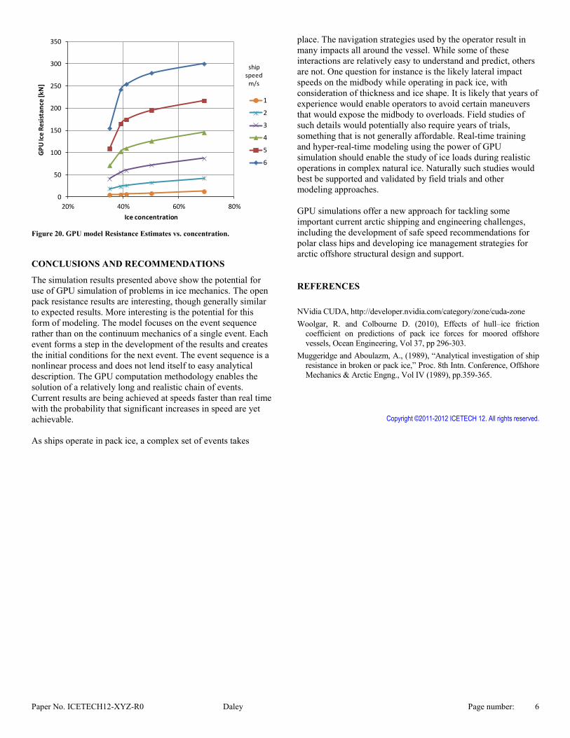
Figure 20 shows the trends vs. ice concentration. One interesting
aspect to note is that the relationship is close to linear at slower
speeds and becomes much less so at higher speed. This could be
the result of the change in the size of the action zone as speed
increases.
Paper No. ICETECH12-XYZ-R0 Daley Page number: 6
0
50
100
150
200
250
300
350
20% 40% 60% 80%
GP
U Ic
e R
esis
tan
ce [k
N]
Ice concentration
1
2
3
4
5
6
ship speed
m/s
Figure 20. GPU model Resistance Estimates vs. concentration.
CONCLUSIONS AND RECOMMENDATIONS
The simulation results presented above show the potential for
use of GPU simulation of problems in ice mechanics. The open
pack resistance results are interesting, though generally similar
to expected results. More interesting is the potential for this
form of modeling. The model focuses on the event sequence
rather than on the continuum mechanics of a single event. Each
event forms a step in the development of the results and creates
the initial conditions for the next event. The event sequence is a
nonlinear process and does not lend itself to easy analytical
description. The GPU computation methodology enables the
solution of a relatively long and realistic chain of events.
Current results are being achieved at speeds faster than real time
with the probability that significant increases in speed are yet
achievable.
As ships operate in pack ice, a complex set of events takes
place. The navigation strategies used by the operator result in
many impacts all around the vessel. While some of these
interactions are relatively easy to understand and predict, others
are not. One question for instance is the likely lateral impact
speeds on the midbody while operating in pack ice, with
consideration of thickness and ice shape. It is likely that years of
experience would enable operators to avoid certain maneuvers
that would expose the midbody to overloads. Field studies of
such details would potentially also require years of trials,
something that is not generally affordable. Real-time training
and hyper-real-time modeling using the power of GPU
simulation should enable the study of ice loads during realistic
operations in complex natural ice. Naturally such studies would
best be supported and validated by field trials and other
modeling approaches.
GPU simulations offer a new approach for tackling some
important current arctic shipping and engineering challenges,
including the development of safe speed recommendations for
polar class hips and developing ice management strategies for
arctic offshore structural design and support.
REFERENCES
NVidia CUDA, http://developer.nvidia.com/category/zone/cuda-zone
Woolgar, R. and Colbourne D. (2010), Effects of hull–ice friction
coefficient on predictions of pack ice forces for moored offshore
vessels, Ocean Engineering, Vol 37, pp 296-303.
Muggeridge and Aboulazm, A., (1989), “Analytical investigation of ship
resistance in broken or pack ice,” Proc. 8th Intn. Conference, Offshore
Mechanics & Arctic Engng., Vol IV (1989), pp.359-365.
Copyright ©2011-2012 ICETECH 12. All rights reserved.