GPS, Glonass, Galileo Receiver testing Using a - Inside GNSS
GPS, Glonass, Galileo, BeiDou Receiver Testing Using a GNSS Signal Simulator Application Note
Products:
| R&SSMBV100A
Testing global navigation satellite system
(GNSS) receivers can be done easily,
reliably and cost-efficiently by using the
R&S®SMBV100A vector signal generator.
This GNSS simulator can generate GPS,
Glonass, Galileo and BeiDou signals for
up to 24 satellites in realtime.
This application note explains how to
perform automated receiver tests using
the R&S®SMBV100A. The presented tests
include TTFF, sensitivity and location
accuracy measurements, moving receiver
and interference tests, and many more.
Basic remote control examples are
provided for the individual tests to ease
programming.
This application note also includes a short
guide for parsing NMEA data.
App
licat
ion
Not
e
C. T
röst
er-S
chm
id
06.2
014-
1GP
86_2
E
Table of Contents
1GP86_2E Rohde & Schwarz GPS, Glonass, Galileo, BeiDou Receiver Testing Using a GNSS Signal Simulator 2
Table of Contents
1 Note ......................................................................................... 4
2 Introduction ............................................................................ 4
3 GNSS Signal Simulation ........................................................ 5
3.1 Advantages of Simulation over Real GNSS Satellite Signals .................. 5
3.2 Rohde & Schwarz GNSS Signal Simulator ................................................ 6
3.2.1 You Need More Than 24 Satellites?............................................................ 8
4 Test Setup ............................................................................... 9
4.1 Radiation ....................................................................................................... 9
4.2 Direct Connection ......................................................................................10
4.3 Complete Setup ..........................................................................................12
4.4 Sometimes Receivers Know Too Much… ................................................13
5 GNSS Receiver Testing ....................................................... 15
5.2 Time To First Fix .........................................................................................19
5.3 Reacquisition Time ....................................................................................21
5.4 Sensitivity ....................................................................................................23
5.4.1 Sensitivity Testing in Production .............................................................23
5.4.2 Sensitivity Testing in R&D .........................................................................25
5.4.2.1 Static Satellites ...........................................................................................25
5.4.2.2 Dynamic Satellites (Constellation) ...........................................................28
5.5 Location Accuracy .....................................................................................30
5.5.1 Static Location Accuracy ..........................................................................31
5.5.2 Dynamic Location Accuracy .....................................................................32
5.6 Moving Receiver .........................................................................................33
5.7 Long-Term Experiment ..............................................................................37
5.8 Interference .................................................................................................39
5.9 Multipath Reception ...................................................................................40
5.10 Atmospheric Modeling ...............................................................................43
5.11 Leap Second Insertion ...............................................................................45
5.12 1PPS Signal .................................................................................................46
6 Features Worth Considering… ........................................... 48
Table of Contents
1GP86_2E Rohde & Schwarz GPS, Glonass, Galileo, BeiDou Receiver Testing Using a GNSS Signal Simulator 3
6.1 Change Settings Without Interrupting Signal Generation .....................48
6.2 Query Time-Specific Information ..............................................................49
7 Parsing NMEA Data .............................................................. 50
8 Summary ............................................................................... 55
9 Abbreviations ....................................................................... 56
10 References ............................................................................ 57
11 Ordering Information ........................................................... 57
Note
1GP86_2E Rohde & Schwarz GPS, Glonass, Galileo, BeiDou Receiver Testing Using a GNSS Signal Simulator 4
1 Note The abbreviation “SMBV” is used in this application note for the Rohde & Schwarz
product R&S®SMBV100A.
As the GNSS simulation capabilities of the SMBV are being enhanced successively,
some features presented in this application note may have been improved or added
since the last release of this document. Therefore, please note the release date of this
application note, because it is updated from time to time.
2 Introduction Global navigation satellite system (GNSS) technology has become an integral part of
our daily life. The range of applications spans consumer, industrial, automotive and
military sectors. The importance of GNSS continues to increase, as there is potential
for even more. The trend is clear, and new satellite systems are being deployed
around the world. In the consumer market, receivers are becoming more and more
widespread, since they are vitally used in cars and mobile terminals for navigation and
positioning.
These receivers can be tested easily, reliably and cost-efficiently by using a GNSS
simulator such as the SMBV from Rohde & Schwarz. GPS, Glonass, Galileo, and
BeiDou signals for up to 24 satellites can be generated in realtime with a single
standalone instrument that can even support other digital standards such as LTE and
WLAN. This sets new standards in the field of satellite simulation for R&D and
production.
The purpose of this application note is to explain how to perform automated receiver
tests using the SMBV. Although the SMBV can simulate different satellite systems in
parallel (hybrid constellation) in a straightforward way, we will focus on non-hybrid
scenarios to keep the examples simple. Generally, the given examples are kept
generic to a certain extent to serve as a basis for user-specific versions.
This application note starts by pointing out the advantages of GNSS simulation and
briefly presenting the SMBV and its key features (section 3). The test setup is
described in detail in section 4. Section 5 contains various fundamental receiver tests
including time to first fix, sensitivity and location accuracy measurements as well as
moving receiver and interference tests, each described in a separate subsection. A
basic remote control example is given in each of these sections to show how to
configure the SMBV for a particular test. In section 6, we present some instrument
features that are worth considering when operating the SMBV in an automated test
setup. A short guide for parsing recorded receiver data (in NMEA format) is given in
section 7. The application note closes with a short summary.
GNSS Signal Simulation
1GP86_2E Rohde & Schwarz GPS, Glonass, Galileo, BeiDou Receiver Testing Using a GNSS Signal Simulator 5
3 GNSS Signal Simulation
3.1 Advantages of Simulation over Real GNSS Satellite
Signals
One approach to testing a GNSS receiver is to use real satellite signals. The receiver
is equipped with an antenna and receives genuine signals from a navigation system.
This approach allows testing of the receiver under real-world conditions including a
multitude of effects, but it has also severe disadvantages. The test conditions vary
strongly and are unknown to a certain degree. This makes it impossible to repeat a test
under the exact same conditions. In addition, the receiver always has to cope with the
full range of real-world effects including restricted satellite visibility, multipath
propagation and interference, to only name a few. Testing under less complex, well-
defined conditions may not be straightforward. In fact, testing with genuine satellite
signals can become quite cumbersome, since it may be necessary to test the receiver
at different times and diverse locations around the world. This not only costs a lot of
time and money. Some tests may even be impractical. For example, tests in parking
decks and street canyons may be rather easy to carry out, but extensive testing at high
altitudes or high velocities (as occur e.g. in aircraft) may be practically impossible.
A GNSS signal simulator can overcome these problems. This instrument generates a
test signal that models the satellite signals and real-world effects as seen by the
receiver in the field. A simulator offers the following benefits:
The generated signals are exactly known. The receiver characteristics can
thus be tested under controlled conditions with absolute certainty
The test conditions can be exactly reproduced. This makes it possible to
repeat a measurement under the exact same conditions over and over again
Comprehensive testing under various conditions, locations and times can be
performed in a laboratory. Even the movement of the receiver along any route
can be simulated in the laboratory
Time and cost savings are enormous. A key receiver characteristic such as
time to first fix can be tested for locations such as Munich, New York, Beijing
and Sydney within a few hours. This is not possible when using real GNSS
signals for testing
The complexity of the test conditions is scalable from basic testing with one
static satellite to realistic multi-GNSS signal simulation with modeling of
multipath and atmospheric effects. For example, this makes it possible to
perform dedicated tests that include certain effects (while blanking others) to
study a certain performance aspect. As a result, the user can gain a more
detailed insight into the performance of the receiver
In contrast to real GNSS signals, the signals generated by a simulator are
virtually noiseless and thus offer the best possible signal-to-noise ratio for
testing. On some simulators (such as the SMBV) the user can set a well-
defined noise contribution
Due to the above reasons, a GNSS signal simulator is the ideal choice for testing the
performance and verifying the proper operation of your GNSS receiver in research and
development (R&D) and production.
GNSS Signal Simulation
1GP86_2E Rohde & Schwarz GPS, Glonass, Galileo, BeiDou Receiver Testing Using a GNSS Signal Simulator 6
3.2 Rohde & Schwarz GNSS Signal Simulator
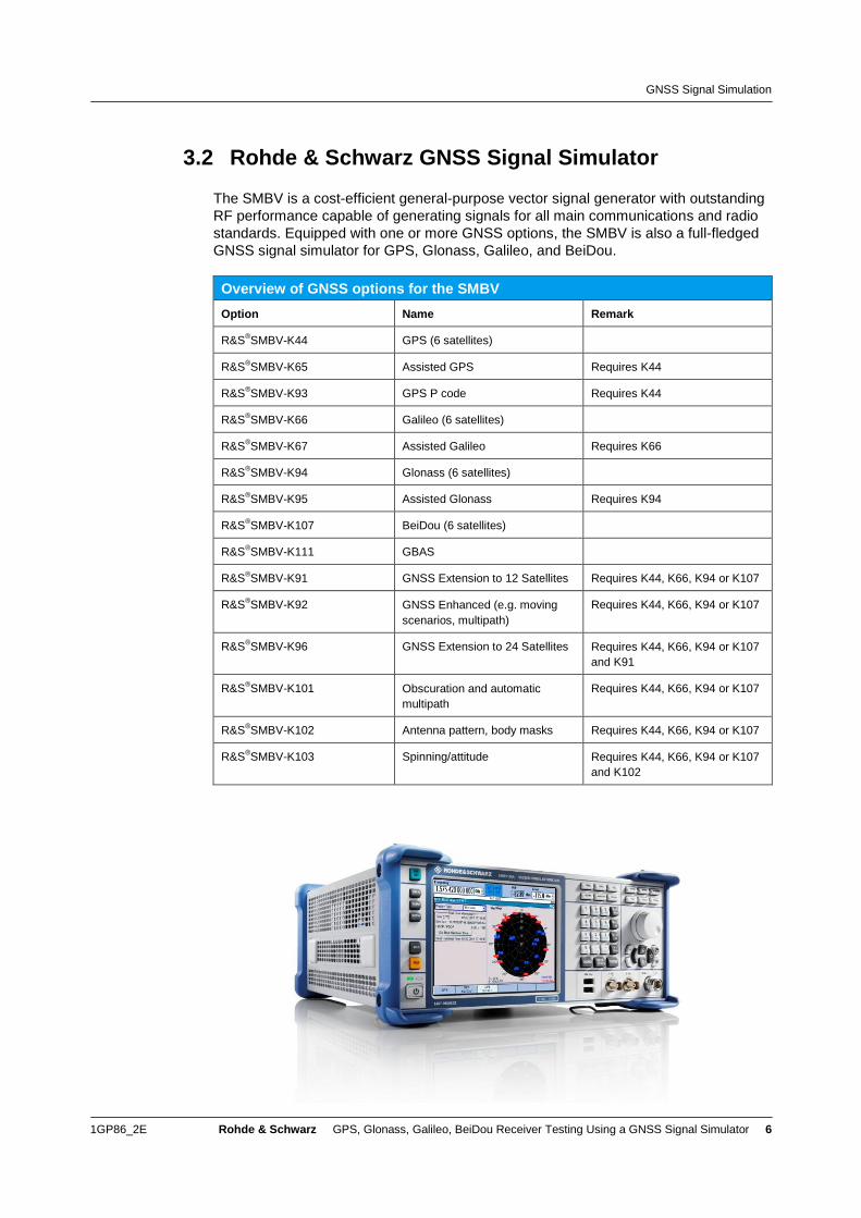
The SMBV is a cost-efficient general-purpose vector signal generator with outstanding
RF performance capable of generating signals for all main communications and radio
standards. Equipped with one or more GNSS options, the SMBV is also a full-fledged
GNSS signal simulator for GPS, Glonass, Galileo, and BeiDou.
Overview of GNSS options for the SMBV
Option Name Remark
R&S®SMBV-K44 GPS (6 satellites)
R&S®SMBV-K65 Assisted GPS Requires K44
R&S®SMBV-K93 GPS P code Requires K44
R&S®SMBV-K66 Galileo (6 satellites)
R&S®SMBV-K67 Assisted Galileo Requires K66
R&S®SMBV-K94 Glonass (6 satellites)
R&S®SMBV-K95 Assisted Glonass Requires K94
R&S®SMBV-K107 BeiDou (6 satellites)
R&S®SMBV-K111 GBAS
R&S®SMBV-K91 GNSS Extension to 12 Satellites Requires K44, K66, K94 or K107
R&S®SMBV-K92 GNSS Enhanced (e.g. moving
scenarios, multipath)
Requires K44, K66, K94 or K107
R&S®SMBV-K96 GNSS Extension to 24 Satellites Requires K44, K66, K94 or K107
and K91
R&S®SMBV-K101 Obscuration and automatic
multipath
Requires K44, K66, K94 or K107
R&S®SMBV-K102 Antenna pattern, body masks Requires K44, K66, K94 or K107
R&S®SMBV-K103 Spinning/attitude Requires K44, K66, K94 or K107
and K102
GNSS Signal Simulation
1GP86_2E Rohde & Schwarz GPS, Glonass, Galileo, BeiDou Receiver Testing Using a GNSS Signal Simulator 7
The SMBV is a powerful one-box solution for reliable and flexible GNSS receiver
testing. It offers the following key features:
Realtime GNSS signal generation for GPS L1/L2 (C/A and P code), Glonass
L1/L2, Galileo E1, and BeiDou L1.
Simulation of up to 24 satellites
Unlimited simulation time with automatic, on-the-fly exchange of satellites
Simulation of static satellite signals with zero or constant Doppler shift
Simulation of hybrid GPS, Glonass, Galileo, and BeiDou satellite constellations
as seen by today’s GNSS receivers in the real world
Stationary receiver simulation with custom or predefined geographic location
(various cities around the world)
Moving receiver simulation along predefined or user trajectory (with the
possibility to directly import NMEA and KML data)
Hardware in the loop (HIL) operation for realtime position and attitude update
Dynamic and realtime power control for individual or all satellites to simulate
obstructed satellite visibility (shadowing). Activation/deactivation of satellites in
realtime without interrupting signal generation
Simulation of multipath propagation (with configurable delay, power, Doppler
shift and carrier phase for each satellite signal echo)
Automatic obscuration and multipath simulation with predefined and user-
specific scenarios to emulate real-world conditions
Modeling of ionospheric and tropospheric effects on the satellite signal
propagation
Antenna pattern and predefined body masks for all common vehicles
Attitude simulation and spinning
Import of almanac files for up-to-date and historic satellite orbits
Import of RINEX files for up-to-date and historic ephemeris data (up to 12
ephemeris sets)
Support of pre- and user-defined Assisted GPS (A-GPS) test scenarios
including generation of assistance data
Standalone one-box solution – no external software required, no additional PC
needed
In addition to GNSS signal generation, the SMBV also supports standard-compliant
signal generation for digital communications standards such as GSM/EDGE, 3GPP
with HSPA, LTE, WLAN, WiMAX, Bluetooth®, etc., and radio standards such as FM
stereo (with RDS), HD RadioTM
, Sirius and XM Satellite Radio, and DAB. Since today’s
mobile phones implement a number of the above communications standards in
addition to GPS, it is definitely a benefit to have a single, handy instrument that can
generate all of the necessary test signals – all in realtime and without the need of
external software.
The SMBV can be equipped with an additive white Gaussian noise (AWGN) generator
for superimposing noise on the RF output signal in a controlled and deterministic way.
It is also possible to superimpose a CW jamming signal.
All instrument settings can be set remotely using SCPI commands. It is thus possible
to use the SMBV for automated tests executed in production and also during R&D.
Remote control is possible via Ethernet LAN (TCP/IP), GPIB (IEC/IEEE) and USB.
GNSS Signal Simulation
1GP86_2E Rohde & Schwarz GPS, Glonass, Galileo, BeiDou Receiver Testing Using a GNSS Signal Simulator 8
3.2.1 You Need More Than 24 Satellites?
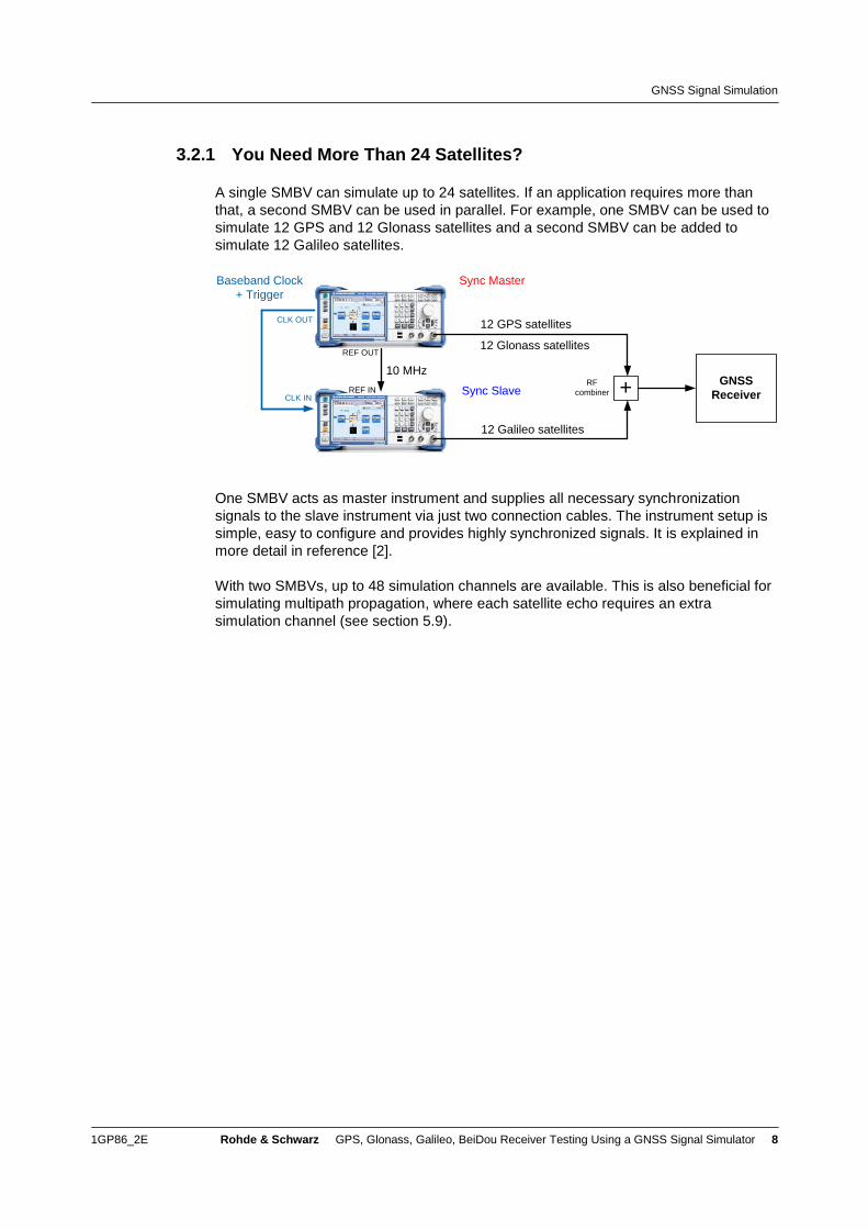
A single SMBV can simulate up to 24 satellites. If an application requires more than
that, a second SMBV can be used in parallel. For example, one SMBV can be used to
simulate 12 GPS and 12 Glonass satellites and a second SMBV can be added to
simulate 12 Galileo satellites.
10 MHz
Baseband Clock
+ Trigger
Sync Master
Sync Slave
CLK OUT
CLK IN
REF OUT
REF INGNSS
Receiver+
12 GPS satellites
12 Galileo satellites
12 Glonass satellites
RF
combiner
One SMBV acts as master instrument and supplies all necessary synchronization
signals to the slave instrument via just two connection cables. The instrument setup is
simple, easy to configure and provides highly synchronized signals. It is explained in
more detail in reference [2].
With two SMBVs, up to 48 simulation channels are available. This is also beneficial for
simulating multipath propagation, where each satellite echo requires an extra
simulation channel (see section 5.9).
Test Setup
1GP86_2E Rohde & Schwarz GPS, Glonass, Galileo, BeiDou Receiver Testing Using a GNSS Signal Simulator 9
GNSS
receiver
GNSS
receiver
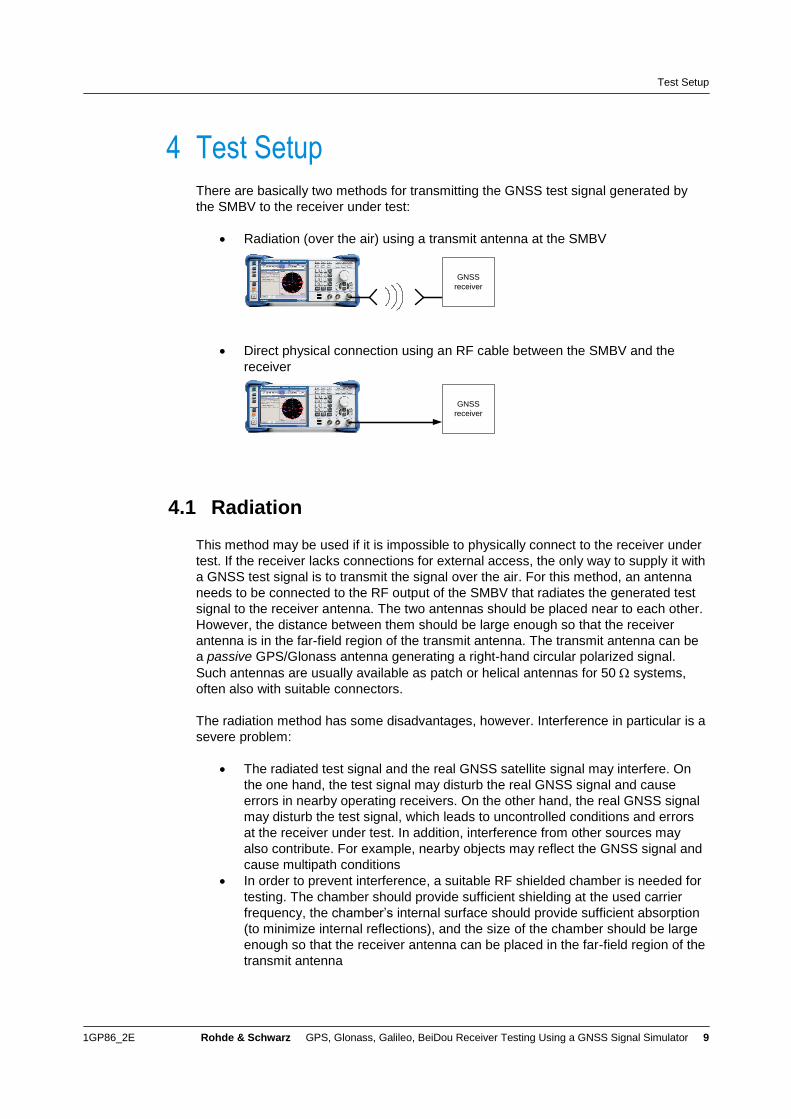
4 Test Setup There are basically two methods for transmitting the GNSS test signal generated by
the SMBV to the receiver under test:
Radiation (over the air) using a transmit antenna at the SMBV
Direct physical connection using an RF cable between the SMBV and the
receiver
4.1 Radiation
This method may be used if it is impossible to physically connect to the receiver under
test. If the receiver lacks connections for external access, the only way to supply it with
a GNSS test signal is to transmit the signal over the air. For this method, an antenna
needs to be connected to the RF output of the SMBV that radiates the generated test
signal to the receiver antenna. The two antennas should be placed near to each other.
However, the distance between them should be large enough so that the receiver
antenna is in the far-field region of the transmit antenna. The transmit antenna can be
a passive GPS/Glonass antenna generating a right-hand circular polarized signal.
Such antennas are usually available as patch or helical antennas for 50 systems,
often also with suitable connectors.
The radiation method has some disadvantages, however. Interference in particular is a
severe problem:
The radiated test signal and the real GNSS satellite signal may interfere. On
the one hand, the test signal may disturb the real GNSS signal and cause
errors in nearby operating receivers. On the other hand, the real GNSS signal
may disturb the test signal, which leads to uncontrolled conditions and errors
at the receiver under test. In addition, interference from other sources may
also contribute. For example, nearby objects may reflect the GNSS signal and
cause multipath conditions
In order to prevent interference, a suitable RF shielded chamber is needed for
testing. The chamber should provide sufficient shielding at the used carrier
frequency, the chamber’s internal surface should provide sufficient absorption
(to minimize internal reflections), and the size of the chamber should be large
enough so that the receiver antenna can be placed in the far-field region of the
transmit antenna
Test Setup
1GP86_2E Rohde & Schwarz GPS, Glonass, Galileo, BeiDou Receiver Testing Using a GNSS Signal Simulator 10
The calibration of the power level at the receiver antenna is difficult. Reliable
sensitivity tests are therefore difficult to perform
The receiver cannot be tested standalone, i.e. without receive antenna. The
test results will contain receiver as well as antenna characteristics
Open radiation of the test signal is not a very controlled and robust method. For this
reason, we focus on a direct physical connection with an RF cable. This method
ensures that the signal is transferred from the SMBV to the receiver without
interference.
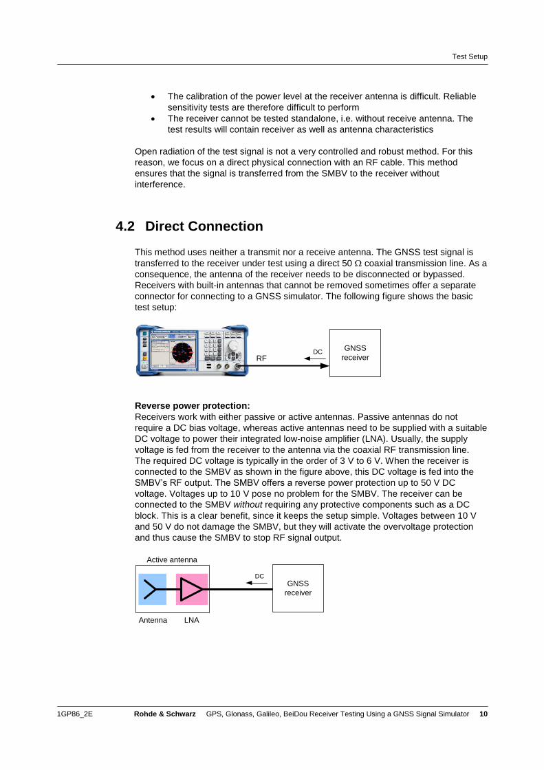
4.2 Direct Connection
This method uses neither a transmit nor a receive antenna. The GNSS test signal is
transferred to the receiver under test using a direct 50 coaxial transmission line. As a
consequence, the antenna of the receiver needs to be disconnected or bypassed.
Receivers with built-in antennas that cannot be removed sometimes offer a separate
connector for connecting to a GNSS simulator. The following figure shows the basic
test setup:
GNSS
receiverRFDC
Reverse power protection:
Receivers work with either passive or active antennas. Passive antennas do not
require a DC bias voltage, whereas active antennas need to be supplied with a suitable
DC voltage to power their integrated low-noise amplifier (LNA). Usually, the supply
voltage is fed from the receiver to the antenna via the coaxial RF transmission line.
The required DC voltage is typically in the order of 3 V to 6 V. When the receiver is
connected to the SMBV as shown in the figure above, this DC voltage is fed into the
SMBV’s RF output. The SMBV offers a reverse power protection up to 50 V DC
voltage. Voltages up to 10 V pose no problem for the SMBV. The receiver can be
connected to the SMBV without requiring any protective components such as a DC
block. This is a clear benefit, since it keeps the setup simple. Voltages between 10 V
and 50 V do not damage the SMBV, but they will activate the overvoltage protection
and thus cause the SMBV to stop RF signal output.
Active antenna
Antenna LNA
GNSS
receiver
DC
Test Setup
1GP86_2E Rohde & Schwarz GPS, Glonass, Galileo, BeiDou Receiver Testing Using a GNSS Signal Simulator 11
Cables:
To connect the receiver to the SMBV, use suitable, good-quality cables exhibiting low
loss at GNSS frequencies. Any loss occurring along the transmission line can be
compensated by setting a correspondingly higher level in the SMBV. The RF level can
be set with a resolution of 0.01 dB over the entire dynamic range of the SMBV. To
achieve a high level accuracy at the receiver under test, the cable loss should be
known precisely either from the cable’s specifications or a calibration measurement.
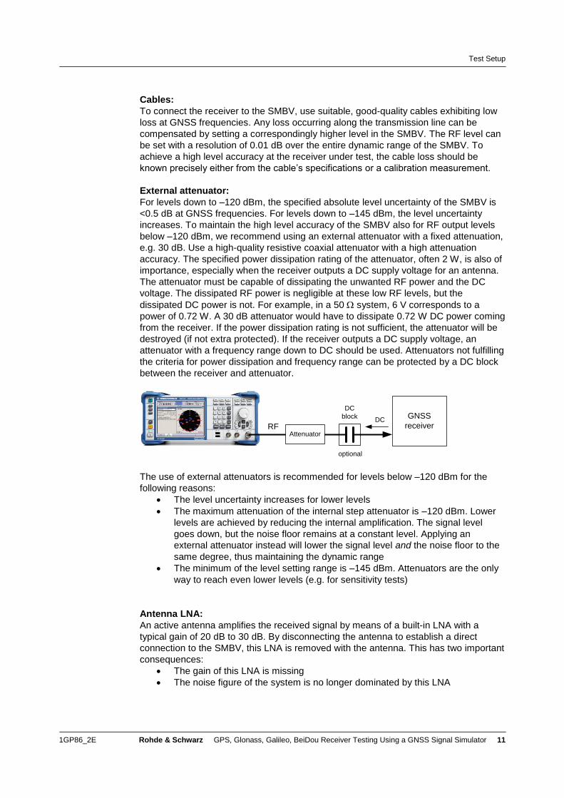
External attenuator:
For levels down to –120 dBm, the specified absolute level uncertainty of the SMBV is
<0.5 dB at GNSS frequencies. For levels down to –145 dBm, the level uncertainty
increases. To maintain the high level accuracy of the SMBV also for RF output levels
below –120 dBm, we recommend using an external attenuator with a fixed attenuation,
e.g. 30 dB. Use a high-quality resistive coaxial attenuator with a high attenuation
accuracy. The specified power dissipation rating of the attenuator, often 2 W, is also of
importance, especially when the receiver outputs a DC supply voltage for an antenna.
The attenuator must be capable of dissipating the unwanted RF power and the DC
voltage. The dissipated RF power is negligible at these low RF levels, but the
dissipated DC power is not. For example, in a 50 system, 6 V corresponds to a
power of 0.72 W. A 30 dB attenuator would have to dissipate 0.72 W DC power coming
from the receiver. If the power dissipation rating is not sufficient, the attenuator will be
destroyed (if not extra protected). If the receiver outputs a DC supply voltage, an
attenuator with a frequency range down to DC should be used. Attenuators not fulfilling
the criteria for power dissipation and frequency range can be protected by a DC block
between the receiver and attenuator.
RFAttenuator
GNSS
receiverDC
DC
block
optional
The use of external attenuators is recommended for levels below –120 dBm for the
following reasons:
The level uncertainty increases for lower levels
The maximum attenuation of the internal step attenuator is –120 dBm. Lower
levels are achieved by reducing the internal amplification. The signal level
goes down, but the noise floor remains at a constant level. Applying an
external attenuator instead will lower the signal level and the noise floor to the
same degree, thus maintaining the dynamic range
The minimum of the level setting range is –145 dBm. Attenuators are the only
way to reach even lower levels (e.g. for sensitivity tests)
Antenna LNA:
An active antenna amplifies the received signal by means of a built-in LNA with a
typical gain of 20 dB to 30 dB. By disconnecting the antenna to establish a direct
connection to the SMBV, this LNA is removed with the antenna. This has two important
consequences:
The gain of this LNA is missing
The noise figure of the system is no longer dominated by this LNA
Test Setup
1GP86_2E Rohde & Schwarz GPS, Glonass, Galileo, BeiDou Receiver Testing Using a GNSS Signal Simulator 12
The missing gain can be easily compensated by the SMBV without any restriction on
the dynamic range of the simulator. Just increase the RF output level of the SMBV as
needed to provide the receiver with the proper input level.
Generally, the antenna LNA, i.e. the first amplifier in a chain of cascaded amplifiers,
dominates the noise figure of the entire system. The noise figure of the antenna LNA is
typically 1.5 dB to 1.8 dB. By removing this LNA, the second amplifier in a chain now
dominates the noise figure of the system. Often, this amplifier has a worse noise figure
than the antenna LNA. This fact can have an impact on receiver sensitivity tests, e.g.
when satellite C/N ratios are read from the receiver and validated. The dependency of
the reported C/N ratios on the noise figure of the system should be taken into account
when defining the test limits. To re-establish the noise figure of the original system, an
external LNA with the same noise figure (and similar gain) as the removed LNA can be
used in the setup as a replacement for the antenna’s built-in LNA.
GNSS
receiverRF
LNA
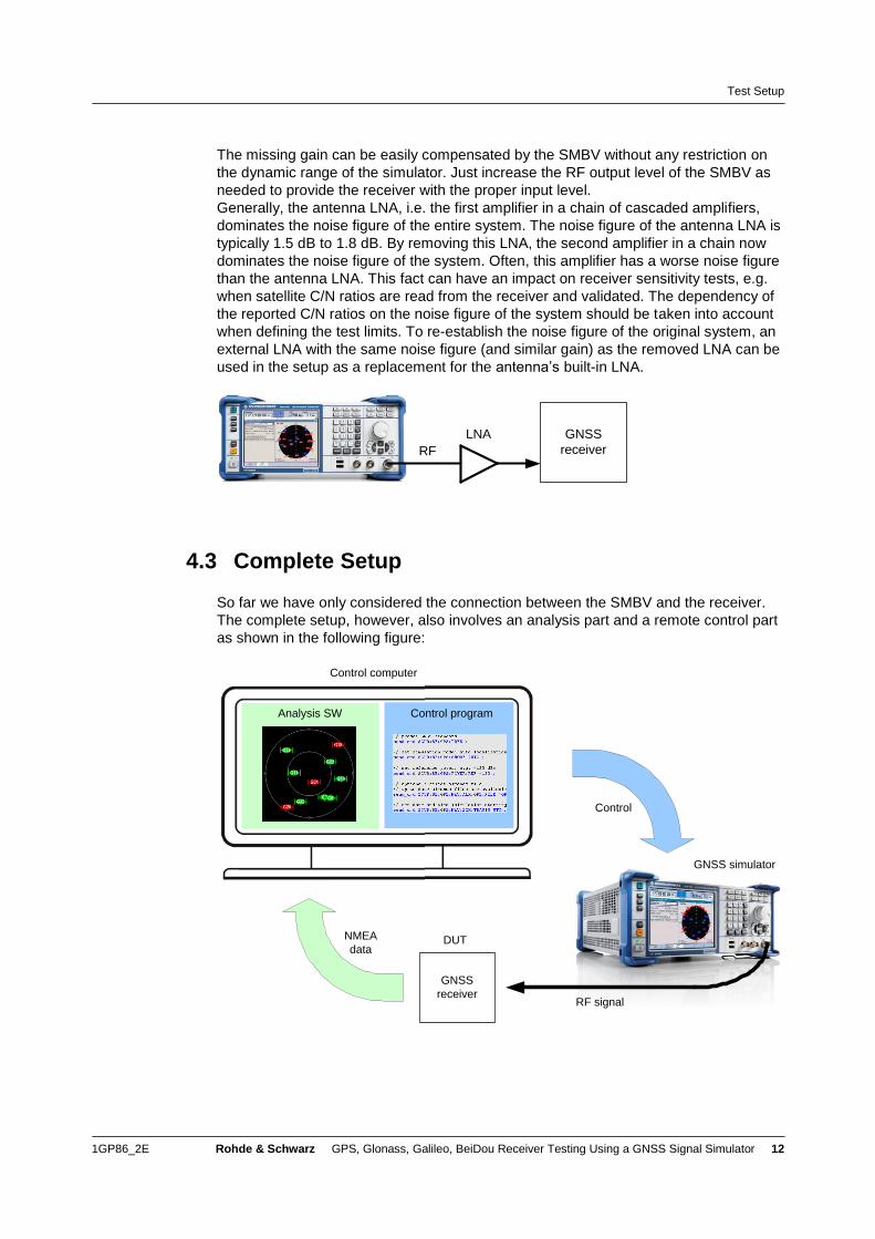
4.3 Complete Setup
So far we have only considered the connection between the SMBV and the receiver.
The complete setup, however, also involves an analysis part and a remote control part
as shown in the following figure:
Control computer
Control programAnalysis SW
Control
GNSS simulator
GNSS
receiver
NMEA
dataDUT
RF signal
Test Setup
1GP86_2E Rohde & Schwarz GPS, Glonass, Galileo, BeiDou Receiver Testing Using a GNSS Signal Simulator 13
SMBV remote control part:
The SMBV can be controlled either manually via the instrument GUI or remotely.
Remote control requires a control computer connected to the SMBV via LAN, GPIB or
USB (see reference [6] for details). For example, it is possible to remote-control the
SMBV in two ways:
Via a remote desktop connection over LAN. In this case, the settings are made
manually via the remote instrument GUI. (VNC software is installed on the
SMBV, so the control PC just requires a browser to connect)
Via an automated test program. In this case, the settings are made
programmatically using SCPI commands
Analysis part:
The receiver under test usually reports its results in the standardized NMEA data
format. This data can be read in and processed by third-party software that makes it
possible to analyze, visualize and log the data. Many vendors provide special
evaluation software of this kind for their receivers. The software usually also allows the
user to control the receiver, e.g. to initialize a cold start. (Generally, the control of the
receiver is device-specific and thus beyond the scope of this application note.)
4.4 Sometimes Receivers Know Too Much…
As time constantly passes, the date and time information transmitted by real satellite
signals only advances and never reverses. Some receivers rely on this physical law to
validate their results: A receiver that has acquired a certain date and time “knows” that
it is not possible to go back in time, although simulated satellite signals may indicate
something else. Such a receiver will refuse to accept the time stamp in the past and
interpret it as an erroneous result. Similarly, a receiver that has acquired a location fix
“knows” from the almanac which satellites are visible at that location. Although
simulated satellite signals may show that the receiver has moved around half the world
in just a few minutes, the receiver will still search for the known satellites, which are,
however, not visible at the new, distant location. The receiver will thus fail to acquire a
position fix. Normally, the validation mechanisms help to reduce navigation errors, but
can be disadvantageous when working with a GNSS simulator.
From the simulator’s side, it is no problem to simulate a point in time, e.g. Sept. 23,
2011, 4:00 p.m., again and again. Also stepping back in time and simulating a time
point years ago, e.g. in 2002, is no problem at all. The same applies for the location;
the simulator can emulate the satellite signals as received in e.g. Munich and a minute
later as received in e.g. Beijing. From the receiver’s side, however, this may cause
problems, for example if internal protocol checks validate the obtained time data.
These problems can be overcome by making the receiver forget the current date and
time, where it is located at the moment and where the satellites are orbiting. This is
done by cold-starting receiver, which erases information about the current time and
position as well as almanac data.
One distinguishes between cold, warm and hot starts of a receiver. The following table
gives an overview:
Test Setup
1GP86_2E Rohde & Schwarz GPS, Glonass, Galileo, BeiDou Receiver Testing Using a GNSS Signal Simulator 14
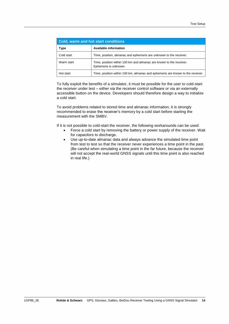
Cold, warm and hot start conditions
Type Available information
Cold start Time, position, almanac and ephemeris are unknown to the receiver.
Warm start Time, position within 100 km and almanac are known to the receiver.
Ephemeris is unknown.
Hot start Time, position within 100 km, almanac and ephemeris are known to the receiver.
To fully exploit the benefits of a simulator, it must be possible for the user to cold-start
the receiver under test – either via the receiver control software or via an externally
accessible button on the device. Developers should therefore design a way to initialize
a cold start.
To avoid problems related to stored time and almanac information, it is strongly
recommended to erase the receiver’s memory by a cold start before starting the
measurement with the SMBV.
If it is not possible to cold-start the receiver, the following workarounds can be used:
Force a cold start by removing the battery or power supply of the receiver. Wait
for capacitors to discharge.
Use up-to-date almanac data and always advance the simulated time point
from test to test so that the receiver never experiences a time point in the past.
(Be careful when simulating a time point in the far future, because the receiver
will not accept the real-world GNSS signals until this time point is also reached
in real life.)
GNSS Receiver Testing
1GP86_2E Rohde & Schwarz GPS, Glonass, Galileo, BeiDou Receiver Testing Using a GNSS Signal Simulator 15
5 GNSS Receiver Testing The following sections explain how the SMBV can be used to perform some basic
receiver tests. To determine the receiver’s general performance, some fundamental
parameters are usually measured. The methods and examples presented in this
application note should only be regarded as basic guidelines. There are many
alternative methods to characterize the receiver’s performance. Some tests may be
more relevant than others, depending on the intended application of the receiver. This
application note covers the most common receiver tests but does not provide a
complete set of tests. The following tests are described in the following sections:
Time to first fix measurement
Reacquisition time measurement
Sensitivity measurement
Location accuracy measurement
Testing dynamics of a moving receiver
Long-term stability measurements
Influence of interference
Influence of multipath reception
Influence of atmospheric modeling
Leap second insertion
1PPS signal
The following table gives an overview and a short explanation of some of the
fundamental parameters and technical terms used in this application note.
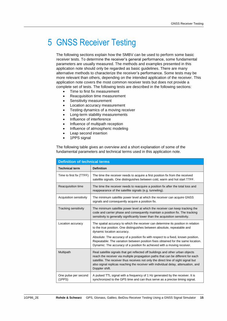
Definition of technical terms
Technical term Definition
Time to first fix (TTFF) The time the receiver needs to acquire a first position fix from the received
satellite signals. One distinguishes between cold, warm and hot start TTFF.
Reacquisition time The time the receiver needs to reacquire a position fix after the total loss and
reappearance of the satellite signals (e.g. tunneling).
Acquisition sensitivity The minimum satellite power level at which the receiver can acquire GNSS
signals and consequently acquire a position fix.
Tracking sensitivity The minimum satellite power level at which the receiver can keep tracking the
code and carrier phase and consequently maintain a position fix. The tracking
sensitivity is generally significantly lower than the acquisition sensitivity.
Location accuracy The spatial accuracy to which the receiver can determine its position in relation
to the true position. One distinguishes between absolute, repeatable and
dynamic location accuracy.
Absolute: The accuracy of a position fix with respect to a fixed, known position.
Repeatable: The variation between position fixes obtained for the same location.
Dynamic: The accuracy of a position fix achieved with a moving receiver.
Multipath Real satellite signals that get reflected off buildings and other urban objects
reach the receiver via multiple propagation paths that can be different for each
satellite. The receiver thus receives not only the direct line of sight signal but
also signal replicas reaching the receiver with individual delay, attenuation, and
Doppler shift.
One pulse per second
(1PPS)
A pulsed TTL signal with a frequency of 1 Hz generated by the receiver. It is
synchronized to the GPS time and can thus serve as a precise timing signal.
GNSS Receiver Testing
1GP86_2E Rohde & Schwarz GPS, Glonass, Galileo, BeiDou Receiver Testing Using a GNSS Signal Simulator 16
The SMBV can be remote-controlled via automated test programs using SCPI
commands. In the following sections, we provide some remote control examples that
are written in a simplified pseudo code syntax:
The fictive function “send_cmd” sends an SCPI command to the SMBV
Fictive functions such as “get_result” query a result from the receiver
Fictive functions such as “calculate_result” call an action (e.g. computation,
analysis)
A comment line is indicated by “//”
To make the code examples easier to read, the following color coding is used:
Blue indicates SMBV-related commands
Green indicates general and receiver-related commands
The GNSS-related SCPI commands start with “SOUR:BB:<GNSS>”, where <GNSS> is
either “GPS” for GPS, “GAL” for Galileo, “BEID” for BeiDou or “GLON” for Glonass. In the
code examples “GPS” is used. However, “GPS” can be replaced by “GAL”, “BEID” or
“GLON” if the other GNSS standards are to be used.
Some general settings apply to all code examples and are therefore mentioned at this
point:
The RF frequency is set via the GNSS standards by setting the parameter “RF
band”.
Example: SOUR:BB:GPS:RFB L1
RF frequency settings made using the command “SOUR:FREQ” are overwritten
as soon as the GNSS signal is turned on.
The RF level is set via the GNSS standards by setting the parameter “Ref.
Power”.
Example: SOUR:BB:GPS:POW:REF -130
Note that this parameter does not set the total RF output level directly but
rather indirectly, as this parameter sets the reference power for the satellite
power levels. The total RF output power depends on additional (configurable)
factors such as the number of satellites, their relative levels, etc. This is
described in greater detail under “Satellite power” on page 17.
RF level settings made using the command “SOUR:POW” are overwritten as
soon as the GNSS signal is turned on.
The RF output is activated using the command “OUTP:STAT ON”.
The baseband generator is activated using the command
“SOUR:BB:GPS:STAT ON”. This command starts baseband signal calculation.
Since the calculation process can take some time, this command should be
followed by a synchronization command such as “*OPC?”. Please see
reference [5] for details and limitations on “*OPC?” and for more sophisticated
synchronization techniques that also allow multi-tasking.
To ensure proper timing of the measurements, the SMBV can be explicitly
triggered manually or remotely to output the GNSS signal (internal triggering).
The trigger mode is set to “Armed Retrigger” using the command SOUR:BB:GPS:TRIG:SEQ ARET
In this mode, every trigger event causes a restart of the GNSS signal. The
trigger event can be issued using the command
GNSS Receiver Testing
1GP86_2E Rohde & Schwarz GPS, Glonass, Galileo, BeiDou Receiver Testing Using a GNSS Signal Simulator 17
SOUR:BB:GPS:TRIG:EXEC
This command actually starts the GNSS signal. The signal can be stopped by
using the command SOUR:BB:GPS:TRIG:ARM:EXEC
It is also possible to have the SMBV triggered by an external signal (external
triggering).
For general information and tips about SCPI programming, see also application note
“Top Ten SCPI Programming Tips for Signal Generators” (reference [5]).
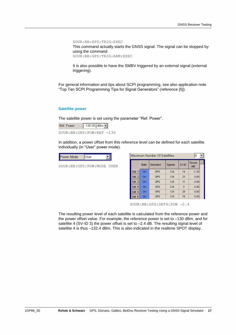
Satellite power
The satellite power is set using the parameter “Ref. Power”.
SOUR:BB:GPS:POW:REF -130
In addition, a power offset from this reference level can be defined for each satellite
individually (in “User” power mode).
SOUR:BB:GPS:POW:MODE USER
SOUR:BB:GPS:SAT4:POW -2.4
The resulting power level of each satellite is calculated from the reference power and
the power offset value. For example, the reference power is set to –130 dBm, and for
satellite 4 (SV-ID 3) the power offset is set to –2.4 dB. The resulting signal level of
satellite 4 is thus –132.4 dBm. This is also indicated in the realtime SPOT display.
GNSS Receiver Testing
1GP86_2E Rohde & Schwarz GPS, Glonass, Galileo, BeiDou Receiver Testing Using a GNSS Signal Simulator 18
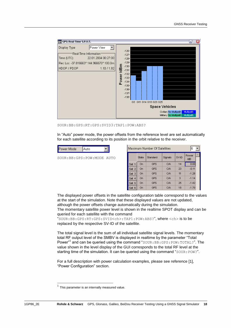
SOUR:BB:GPS:RT:GPS:SVID3:TAP1:POW:ABS?
In “Auto” power mode, the power offsets from the reference level are set automatically
for each satellite according to its position in the orbit relative to the receiver.
SOUR:BB:GPS:POW:MODE AUTO
The displayed power offsets in the satellite configuration table correspond to the values
at the start of the simulation. Note that these displayed values are not updated,
although the power offsets change automatically during the simulation.
The momentary satellite power level is shown in the realtime SPOT display and can be
queried for each satellite with the command
“SOUR:BB:GPS:RT:GPS:SVID<ch>:TAP1:POW:ABS?”, where <ch> is to be
replaced by the respective SV-ID of the satellite.
The total signal level is the sum of all individual satellite signal levels. The momentary
total RF output level of the SMBV is displayed in realtime by the parameter “Total
Power”1 and can be queried using the command “SOUR:BB:GPS:POW:TOTAL?”. The
value shown in the level display of the GUI corresponds to the total RF level at the
starting time of the simulation. It can be queried using the command “SOUR:POW?”.
For a full description with power calculation examples, please see reference [1],
“Power Configuration” section.
1 This parameter is an internally measured value.
GNSS Receiver Testing
1GP86_2E Rohde & Schwarz GPS, Glonass, Galileo, BeiDou Receiver Testing Using a GNSS Signal Simulator 19
As a general rule, it is strongly recommended to do any power leveling via the level-
related settings in the GNSS standard and not via the conventional RF level setting.
Power levels set using the conventional method (“SOUR:POW” command) are
overwritten as soon as the GNSS signal generation (re)starts.
5.2 Time To First Fix
The purpose of this measurement is to test how quickly the receiver can obtain a first
position fix. The TTFF is an important performance parameter, since it strongly impacts
the usability of the receiver.
For this test, the SMBV simulates a realistic satellite constellation for a fixed location.
The “Auto Localization” simulation mode is used, since in this mode the SMBV sets the
satellite configuration automatically. The user can select a location from a number of
predefined cities around the world or enter a user-defined location. The number of
simulated satellites can also be selected, ranging from 4 to 24. The SMBV then
automatically simulates the satellites that offer the best constellation for the selected
location. The SMBV comes with several almanac files to choose from, but the user can
also use up-to-date almanac files available for download on the Internet. For TTFF
tests, the reference level is usually set to a level well above the acquisition sensitivity
level of the receiver.
Configuration of the SMBV for TTFF testing:
// preset GNSS standard
send_cmd(SOUR:BB:GPS:PRES);
// set simulation mode: auto localization
send_cmd(SOUR:BB:GPS:SMODE AUTO);
// set reference power, e.g. -130 dBm
send_cmd(SOUR:BB:GPS:POWER:REF -130);
// optional: select almanac file
// up-to-date almanac files are available on the Internet.
send_cmd(SOUR:BB:GPS:NAV:ALM:GPS:FILE 'GPS_SEM585.txt');
// set date and time (simulation starting point)
send_cmd(SOUR:BB:GPS:NAV:SIM:TBASIS UTC); // set time basis
send_cmd(SOUR:BB:GPS:NAV:SIM:DATE 2011, 09, 23);
send_cmd(SOUR:BB:GPS:NAV:SIM:TIME 8, 15, 46.689);
// select a location: select a city
send_cmd(SOUR:BB:GPS:LOC:SEL "Munich");
// alternatively:
// select a location: select a user location
// send_cmd(SOUR:BB:GPS:LOC:SEL "User Defined");
// send_cmd(SOUR:BB:GPS:LOC:COOR:DEC 90, 180, 5.5);
// set number of satellites: e.g. 6
send_cmd(SOUR:BB:GPS:SAT:COUNT 6);
GNSS Receiver Testing
1GP86_2E Rohde & Schwarz GPS, Glonass, Galileo, BeiDou Receiver Testing Using a GNSS Signal Simulator 20
Usually a TTFF measurement is repeated several times with significantly different
simulated satellite constellations to test the receiver under a broad range of conditions.
The measured TTFFs are finally averaged. To modify the scenario, change one of the
following:
the simulated time (advance by several hours)
or the number of simulated satellites
or the simulated location
Loop
{
// turn on GNSS baseband signal
send_cmd(SOUR:BB:GPS:STAT ON);
send_cmd(*OPC?); // synchronize
send_cmd(SOUR:BB:GPS:TRIG:EXEC); // trigger
// reset receiver: cold start
do_cold_start();
// measure TTFF
TTFF = get_TTFF();
// turn off GNSS baseband signal
send_cmd(SOUR:BB:GPS:STAT OFF);
// modify scenario: advance time by several hours
time_struct = advance_time(time_struct, hours);
// hours is e.g. 6
// structure includes current year, month, day, hour,
minute, second
send_cmd(SOUR:BB:GPS:NAV:SIM:DATE %f, %f, %f; time_struct.year,
time_struct.month, time_struct.day);
send_cmd(SOUR:BB:GPS:NAV:SIM:TIME %f, %f, %f; time_struct.hour,
time_struct.min, time_struct.sec);
}
It is possible to advance or rewind the simulated time. The simulated time point can be
changed in large steps (several hours) but also increments of minutes, as may be
required for warm and hot start TTFF testing.
TTFF measurements can be quite time-consuming, especially cold start TTFF tests,
because it takes some time for the receiver to gather enough information from the
navigation message of the satellite signals. Therefore, TTFF tests are not very
practical for production, but are extremely important during research and verification
stages.
GNSS Receiver Testing
1GP86_2E Rohde & Schwarz GPS, Glonass, Galileo, BeiDou Receiver Testing Using a GNSS Signal Simulator 21
5.3 Reacquisition Time
The purpose of this measurement is to test how quickly the receiver can reacquire the
satellite signals after it has lost all signals for a short period of time. The reacquisition
time is a performance parameter especially important for in-vehicle GNSS receivers.
For example, after leaving a tunnel where all satellite signals were blocked, the
receiver should be able to quickly get a valid position fix and restore navigation
services.
For this test, the SMBV simulates a realistic satellite constellation for a fixed location,
using the “User Localization” simulation mode. This mode gives the user full control
over the simulated satellites. The user can specify the number of satellites and their
individual power levels, and can also select which satellites should be simulated (via
the SV-ID). Alternatively, the SMBV can determine the satellites that form an optimal
constellation for the selected simulation time. For testing the reacquisition time, the
simulated satellites are deactivated to simulate their loss. After some time, they are
reactivated to simulate restored satellite visibility. Note that the satellites can be
(de)activated in realtime without interrupting the running scenario. The user can select
a location from a number of predefined cities around the world or enter a user-defined
location (see section 5.2). The reference level is usually set to a level well above the
acquisition sensitivity level of the receiver.
Configuration of the SMBV for reacquisition time testing:
// preset GNSS standard
send_cmd(SOUR:BB:GPS:PRES);
// set simulation mode: user localization
send_cmd(SOUR:BB:GPS:SMODE USER);
// select a location: select a city
send_cmd(SOUR:BB:GPS:LOC:SEL "Munich");
// set number of satellites: e.g. 6
send_cmd(SOUR:BB:GPS:SAT:COUNT 6);
// set reference power, e.g. -130 dBm
send_cmd(SOUR:BB:GPS:POWER:REF -130);
// set power mode for satellite configuration: auto
send_cmd(SOUR:BB:GPS:POW:MODE AUTO);
// set optimal satellite constellation
send_cmd(SOUR:BB:GPS:GOC); // activates all 6 satellites
// turn on GNSS baseband signal
send_cmd(SOUR:BB:GPS:STAT ON);
send_cmd(*OPC?); // synchronize
send_cmd(SOUR:BB:GPS:TRIG:EXEC); // trigger
// let the receiver acquire a 3D position fix
wait4fix();
// turn off all satellites
GNSS Receiver Testing
1GP86_2E Rohde & Schwarz GPS, Glonass, Galileo, BeiDou Receiver Testing Using a GNSS Signal Simulator 22
send_cmd(SOUR:BB:GPS:SAT1:STAT OFF);
send_cmd(SOUR:BB:GPS:SAT2:STAT OFF);
send_cmd(SOUR:BB:GPS:SAT3:STAT OFF);
send_cmd(SOUR:BB:GPS:SAT4:STAT OFF);
send_cmd(SOUR:BB:GPS:SAT5:STAT OFF);
send_cmd(SOUR:BB:GPS:SAT6:STAT OFF);
// wait until the receiver loses lock
wait4nofix();
// turn on the satellites again
send_cmd(SOUR:BB:GPS:SAT1:STAT ON);
send_cmd(SOUR:BB:GPS:SAT2:STAT ON);
send_cmd(SOUR:BB:GPS:SAT3:STAT ON);
send_cmd(SOUR:BB:GPS:SAT4:STAT ON);
send_cmd(SOUR:BB:GPS:SAT5:STAT ON);
send_cmd(SOUR:BB:GPS:SAT6:STAT ON);
// synchronize
send_cmd(*OPC?);
// measure reacquisition time, i.e. TTFF after signal
interruption
reacq_time = get_TTFF();
To simulate temporarily interrupted or restricted satellite visibility, the user can
turn off individual satellites
reduce the power of each satellites individually
without interrupting the running scenario.
// turn off a subset of the satellites
send_cmd(SOUR:BB:GPS:SAT2:STAT OFF);
send_cmd(SOUR:BB:GPS:SAT4:STAT OFF);
send_cmd(SOUR:BB:GPS:SAT6:STAT OFF);
// set power mode for satellite configuration: user
send_cmd(SOUR:BB:GPS:POW:MODE USER);
// set reduced power for the remaining satellites (in relation
to the reference power)
send_cmd(SOUR:BB:GPS:SAT1:POW -3);
send_cmd(SOUR:BB:GPS:SAT3:POW -10);
send_cmd(SOUR:BB:GPS:SAT5:POW -20);
As an alternative to the above approach, the user can make use of the R&S®SMBV-
K101 “Obscuration and automatic multipath” option of the SMBV. This option makes it
possible to simulate obstacles such as tunnels, bridges, and parking decks causing
temporary full obscuration of all satellite signals. Different obscuration scenarios can
be configured flexibly and conveniently. A detailed description of this feature can be
found in reference [7]. Please see this dedicated application note for further details.
GNSS Receiver Testing
1GP86_2E Rohde & Schwarz GPS, Glonass, Galileo, BeiDou Receiver Testing Using a GNSS Signal Simulator 23
5.4 Sensitivity
The purpose of this measurement is to find out the minimum satellite signal power at
which the receiver is still able to either acquire or track the satellite signals and
consequently establish or maintain a valid position fix. The acquisition and tracking
sensitivity are two of the most important performance parameters of a GNSS receiver.
Although the satellite signal power receivable on the earth’s surface (with clear view) is
at least about –130 dBm as defined by the specification, this level can drop
significantly inside buildings or under tree foliage, for example. However, receivers with
low sensitivity levels (e.g. –160 dBm) can still be operated in areas where the satellite
signals are low in power due to attenuation. The receiver’s sensitivity is thoroughly
tested in R&D and is often the only parameter tested in production.
5.4.1 Sensitivity Testing in Production
Sensitivity tests in production are often carried out using a very simple scenario with
only one static satellite. With just one satellite, it is not possible to obtain a position fix.
Therefore, only the C/N ratio reported by the receiver for the simulated satellite is
evaluated. At a known power level, which can in fact be greater than the actual
sensitivity level, the receiver must report a certain C/N ratio (test limit). This method
saves testing time. Testing with a full position fix, in contrast, takes quite long and is
thus rarely performed in production of commercial receivers.2
To accurately measure the sensitivity level, the applied power at the receiver’s input
must be precisely known. The SMBV simulates a single static satellite, since this
simple scenario makes it possible to precisely determine the applied power. When
setting the reference power at the SMBV, the user needs to take the following into
account:
Cable loss
External attenuator(s) (optional)
Missing (active) antenna (optional)
To compensate cable loss, applied external attenuation and missing antenna gain,
simply set the reference power to a correspondingly higher level:
SMBV reference power = wanted test level + cable loss + external attenuation +
antenna gain
The SMBV generates the static satellite signal at a known power level either in realtime
or via its internal ARB generator from a precalculated waveform. This waveform file
can be generated with the R&S®WinIQSIM2 software and stored on the SMBV’s local
hard drive.
For time-critical production tests, a single test run can be sufficient. The receiver is set
to a special test mode in which it merely measures the satellite C/N ratio. The SMBV is
set to a fixed low power level, and the satellite C/N ratio reported by the receiver is
validated.
2 Testing with position fix (from C/A code) is, however, performed in production of military receivers that
evaluate the P code. Since the P code is one week long, a time reference is needed first.
GNSS Receiver Testing
1GP86_2E Rohde & Schwarz GPS, Glonass, Galileo, BeiDou Receiver Testing Using a GNSS Signal Simulator 24
Configuration of the SMBV for sensitivity testing in production:
Realtime: // preset GNSS standard
send_cmd(SOUR:BB:GPS:PRES);
// set simulation mode: static (default)
send_cmd(SOUR:BB:GPS:SMODE STATIC);
// set number of satellites: 1 (default)
send_cmd(SOUR:BB:GPS:SAT:COUNT 1);
// data source: PRBS (default) for GPS and Galileo
// for Glonass use data source "real navigation data" and set
date and time (proper frequency number is then automatically
set)
send_cmd(SOUR:BB:GPS:NAV:DATA PN9);
// send_cmd(SOUR:BB:GPS:NAV:DATA RND);
// set reference power
test_level = wanted_test_level + level_compensation // dBm
send_cmd(SOUR:BB:GPS:POWER:REF %d; test_level);
// Choose the test level such that a golden device (reference
receiver) would report a C/N ratio of 38 dB-Hz to 40 dB-Hz.
// turn on GNSS baseband signal
send_cmd(SOUR:BB:GPS:STAT ON);
send_cmd(*OPC?); // synchronize
send_cmd(SOUR:BB:GPS:TRIG:EXEC); // trigger
ARB: // preset ARB
send_cmd(SOUR:BB:ARB:PRES);
// load waveform
send_cmd(SOUR:BB:ARB:WAV:SEL "/hdd/WinIQSIM2_GPS_waveform.wv");
send_cmd(*OPC?); // synchronize
// turn on ARB signal
send_cmd(SOUR:BB:ARB:STAT ON);
send_cmd(*OPC?); // synchronize
// set RF power
test_level = wanted_test_level + level_compensation // dBm
send_cmd(SOUR:POW %d; test_level);
// Choose the test level such that a golden device (reference
receiver) would report a C/N ratio of 38 dB-Hz to 40 dB-Hz.
// set RF frequency: L1 + Doppler shift (+ frequency number for
Glonass) as configured in WinIQSIM2 during waveform generation
send_cmd(SOUR:FREQ %d; 1.575422 GHz);
GNSS Receiver Testing
1GP86_2E Rohde & Schwarz GPS, Glonass, Galileo, BeiDou Receiver Testing Using a GNSS Signal Simulator 25
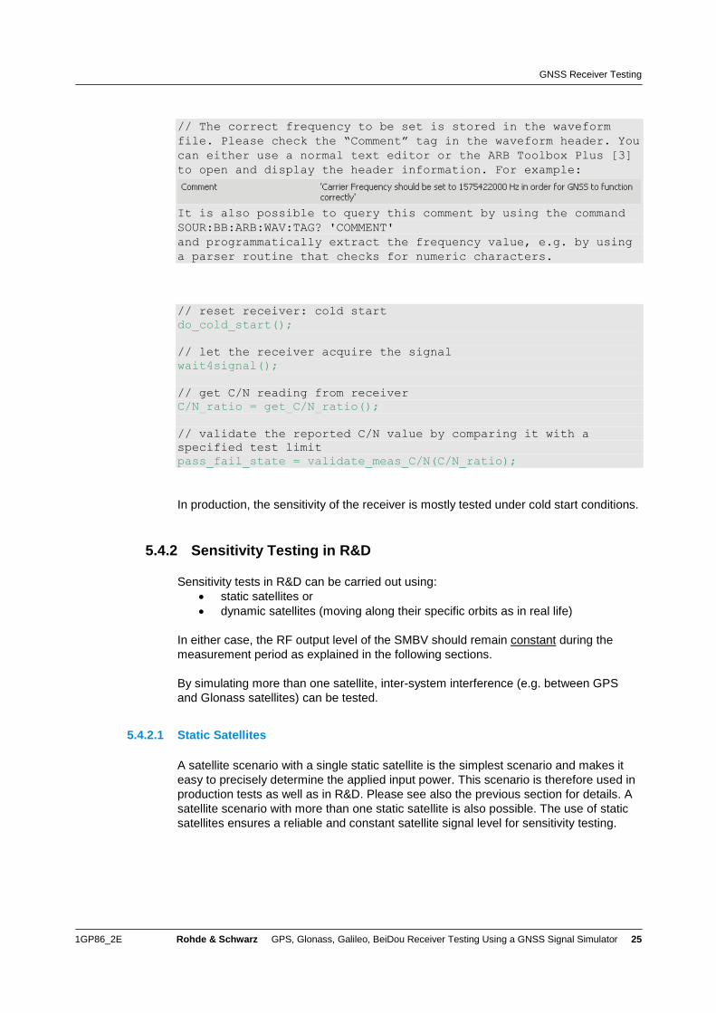
// The correct frequency to be set is stored in the waveform
file. Please check the “Comment” tag in the waveform header. You
can either use a normal text editor or the ARB Toolbox Plus [3]
to open and display the header information. For example:
It is also possible to query this comment by using the command
SOUR:BB:ARB:WAV:TAG? 'COMMENT'
and programmatically extract the frequency value, e.g. by using
a parser routine that checks for numeric characters.
// reset receiver: cold start
do_cold_start();
// let the receiver acquire the signal
wait4signal();
// get C/N reading from receiver
C/N_ratio = get_C/N_ratio();
// validate the reported C/N value by comparing it with a
specified test limit
pass_fail_state = validate_meas_C/N(C/N_ratio);
In production, the sensitivity of the receiver is mostly tested under cold start conditions.
5.4.2 Sensitivity Testing in R&D
Sensitivity tests in R&D can be carried out using:
static satellites or
dynamic satellites (moving along their specific orbits as in real life)
In either case, the RF output level of the SMBV should remain constant during the
measurement period as explained in the following sections.
By simulating more than one satellite, inter-system interference (e.g. between GPS
and Glonass satellites) can be tested.
5.4.2.1 Static Satellites
A satellite scenario with a single static satellite is the simplest scenario and makes it
easy to precisely determine the applied input power. This scenario is therefore used in
production tests as well as in R&D. Please see also the previous section for details. A
satellite scenario with more than one static satellite is also possible. The use of static
satellites ensures a reliable and constant satellite signal level for sensitivity testing.
GNSS Receiver Testing
1GP86_2E Rohde & Schwarz GPS, Glonass, Galileo, BeiDou Receiver Testing Using a GNSS Signal Simulator 26
Since receivers can have sensitivity levels as low as –160 dBm, extremely low signal
levels have to be generated with high level accuracy. To reach such low levels and for
best level accuracy, we recommend using external attenuators (see section 4.2 for
details). When setting the RF level of the SMBV, the user needs to take into account
the applied external attenuation as well as cable losses and possibly missing gain from
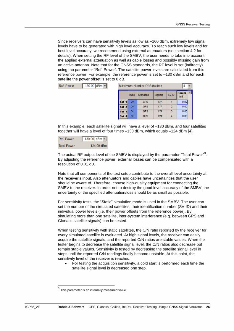
an active antenna. Note that for the GNSS standards, the RF level is set (indirectly)
using the parameter “Ref. Power”. The satellite power levels are calculated from this
reference power. For example, the reference power is set to –130 dBm and for each
satellite the power offset is set to 0 dB.
In this example, each satellite signal will have a level of –130 dBm, and four satellites
together will have a level of four times –130 dBm, which equals –124 dBm [4].
The actual RF output level of the SMBV is displayed by the parameter “Total Power”3.
By adjusting the reference power, external losses can be compensated with a
resolution of 0.01 dB.
Note that all components of the test setup contribute to the overall level uncertainty at
the receiver’s input. Also attenuators and cables have uncertainties that the user
should be aware of. Therefore, choose high-quality equipment for connecting the
SMBV to the receiver. In order not to destroy the good level accuracy of the SMBV, the
uncertainty of the specified attenuation/loss should be as small as possible.
For sensitivity tests, the “Static” simulation mode is used in the SMBV. The user can
set the number of the simulated satellites, their identification number (SV-ID) and their
individual power levels (i.e. their power offsets from the reference power). By
simulating more than one satellite, inter-system interference (e.g. between GPS and
Glonass satellite signals) can be tested.
When testing sensitivity with static satellites, the C/N ratio reported by the receiver for
every simulated satellite is evaluated. At high signal levels, the receiver can easily
acquire the satellite signals, and the reported C/N ratios are stable values. When the
tester begins to decrease the satellite signal level, the C/N ratios also decrease but
remain stable values. Sensitivity is tested by decreasing the satellite signal level in
steps until the reported C/N readings finally become unstable. At this point, the
sensitivity level of the receiver is reached.
For testing the acquisition sensitivity, a cold start is performed each time the
satellite signal level is decreased one step.
3 This parameter is an internally measured value.
GNSS Receiver Testing
1GP86_2E Rohde & Schwarz GPS, Glonass, Galileo, BeiDou Receiver Testing Using a GNSS Signal Simulator 27
For testing the tracking sensitivity, a single cold start is performed at the
beginning of the measurement. Once the receiver has acquired the satellites,
the signal level is decreased without performing further cold starts.
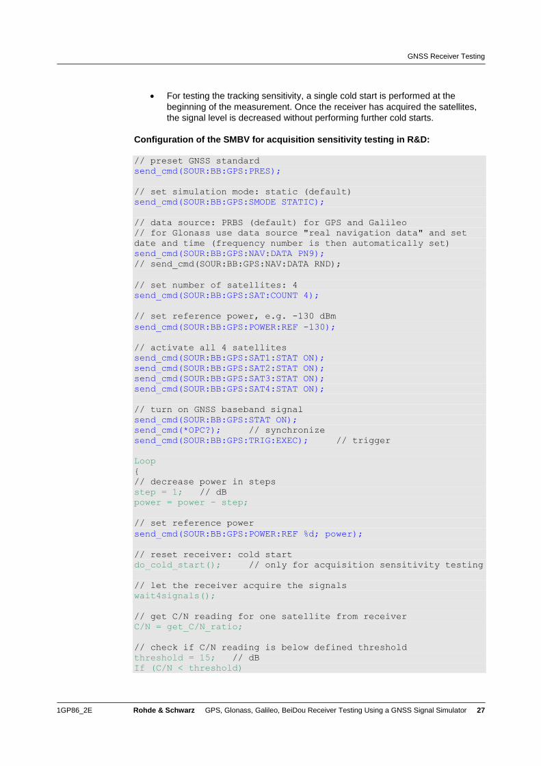
Configuration of the SMBV for acquisition sensitivity testing in R&D:
// preset GNSS standard
send_cmd(SOUR:BB:GPS:PRES);
// set simulation mode: static (default)
send_cmd(SOUR:BB:GPS:SMODE STATIC);
// data source: PRBS (default) for GPS and Galileo
// for Glonass use data source "real navigation data" and set
date and time (frequency number is then automatically set)
send_cmd(SOUR:BB:GPS:NAV:DATA PN9);
// send_cmd(SOUR:BB:GPS:NAV:DATA RND);
// set number of satellites: 4
send_cmd(SOUR:BB:GPS:SAT:COUNT 4);
// set reference power, e.g. -130 dBm
send_cmd(SOUR:BB:GPS:POWER:REF -130);
// activate all 4 satellites
send_cmd(SOUR:BB:GPS:SAT1:STAT ON);
send_cmd(SOUR:BB:GPS:SAT2:STAT ON);
send_cmd(SOUR:BB:GPS:SAT3:STAT ON);
send_cmd(SOUR:BB:GPS:SAT4:STAT ON);
// turn on GNSS baseband signal
send_cmd(SOUR:BB:GPS:STAT ON);
send_cmd(*OPC?); // synchronize
send_cmd(SOUR:BB:GPS:TRIG:EXEC); // trigger
Loop
{
// decrease power in steps
step = 1; // dB
power = power – step;
// set reference power
send_cmd(SOUR:BB:GPS:POWER:REF %d; power);
// reset receiver: cold start
do_cold_start(); // only for acquisition sensitivity testing
// let the receiver acquire the signals
wait4signals();
// get C/N reading for one satellite from receiver
C/N = get_C/N_ratio;
// check if C/N reading is below defined threshold
threshold = 15; // dB
If (C/N < threshold)
GNSS Receiver Testing
1GP86_2E Rohde & Schwarz GPS, Glonass, Galileo, BeiDou Receiver Testing Using a GNSS Signal Simulator 28
{break;} // quit loop
}
// sensitivity level
sens_level = power + step - external_losses;
Please note that changing the reference power (SOUR:BB:GPS:POWER:REF) will
cause the GNSS signal to restart. This is generally no problem when testing the
acquisition sensitivity because the receiver is reset also (cold start). However, the reset
of the GNSS signal may distract tracking sensitivity testing because the receiver can
lose synchronization. In this case, the reference power can be kept constant and
instead the RF level is reduced directly, as an exception.
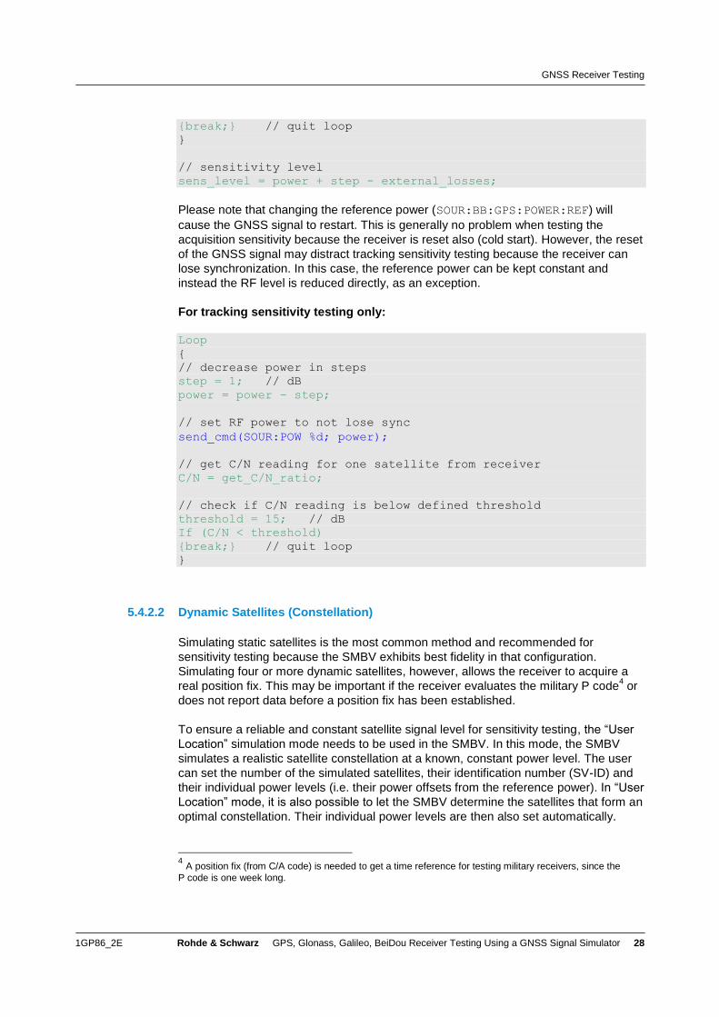
For tracking sensitivity testing only:
Loop
{
// decrease power in steps
step = 1; // dB
power = power – step;
// set RF power to not lose sync
send_cmd(SOUR:POW %d; power);
// get C/N reading for one satellite from receiver
C/N = get_C/N_ratio;
// check if C/N reading is below defined threshold
threshold = 15; // dB
If (C/N < threshold)
{break;} // quit loop
}
5.4.2.2 Dynamic Satellites (Constellation)
Simulating static satellites is the most common method and recommended for
sensitivity testing because the SMBV exhibits best fidelity in that configuration.
Simulating four or more dynamic satellites, however, allows the receiver to acquire a
real position fix. This may be important if the receiver evaluates the military P code4 or
does not report data before a position fix has been established.
To ensure a reliable and constant satellite signal level for sensitivity testing, the “User
Location” simulation mode needs to be used in the SMBV. In this mode, the SMBV
simulates a realistic satellite constellation at a known, constant power level. The user
can set the number of the simulated satellites, their identification number (SV-ID) and
their individual power levels (i.e. their power offsets from the reference power). In “User
Location” mode, it is also possible to let the SMBV determine the satellites that form an
optimal constellation. Their individual power levels are then also set automatically.
4 A position fix (from C/A code) is needed to get a time reference for testing military receivers, since the
P code is one week long.
GNSS Receiver Testing
1GP86_2E Rohde & Schwarz GPS, Glonass, Galileo, BeiDou Receiver Testing Using a GNSS Signal Simulator 29
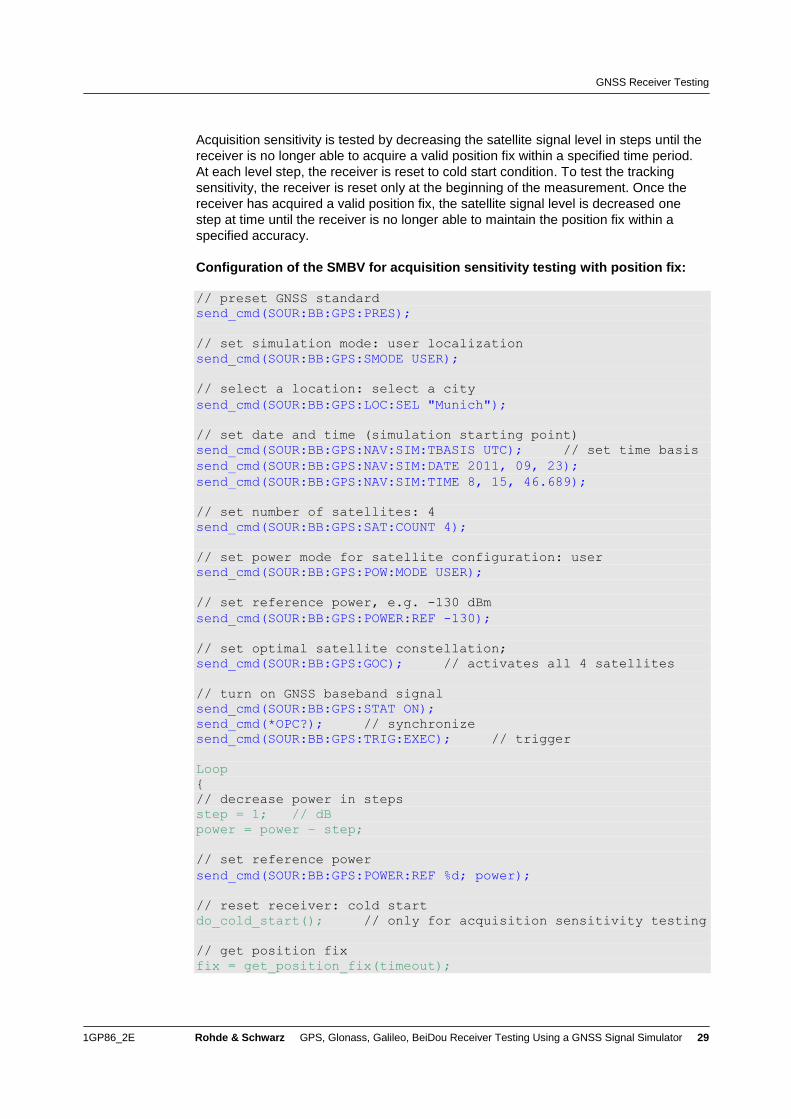
Acquisition sensitivity is tested by decreasing the satellite signal level in steps until the
receiver is no longer able to acquire a valid position fix within a specified time period.
At each level step, the receiver is reset to cold start condition. To test the tracking
sensitivity, the receiver is reset only at the beginning of the measurement. Once the
receiver has acquired a valid position fix, the satellite signal level is decreased one
step at time until the receiver is no longer able to maintain the position fix within a
specified accuracy.
Configuration of the SMBV for acquisition sensitivity testing with position fix:
// preset GNSS standard
send_cmd(SOUR:BB:GPS:PRES);
// set simulation mode: user localization
send_cmd(SOUR:BB:GPS:SMODE USER);
// select a location: select a city
send_cmd(SOUR:BB:GPS:LOC:SEL "Munich");
// set date and time (simulation starting point)
send_cmd(SOUR:BB:GPS:NAV:SIM:TBASIS UTC); // set time basis
send_cmd(SOUR:BB:GPS:NAV:SIM:DATE 2011, 09, 23);
send_cmd(SOUR:BB:GPS:NAV:SIM:TIME 8, 15, 46.689);
// set number of satellites: 4
send_cmd(SOUR:BB:GPS:SAT:COUNT 4);
// set power mode for satellite configuration: user
send_cmd(SOUR:BB:GPS:POW:MODE USER);
// set reference power, e.g. -130 dBm
send_cmd(SOUR:BB:GPS:POWER:REF -130);
// set optimal satellite constellation;
send_cmd(SOUR:BB:GPS:GOC); // activates all 4 satellites
// turn on GNSS baseband signal
send_cmd(SOUR:BB:GPS:STAT ON);
send_cmd(*OPC?); // synchronize
send_cmd(SOUR:BB:GPS:TRIG:EXEC); // trigger
Loop
{
// decrease power in steps
step = 1; // dB
power = power – step;
// set reference power
send_cmd(SOUR:BB:GPS:POWER:REF %d; power);
// reset receiver: cold start
do_cold_start(); // only for acquisition sensitivity testing
// get position fix
fix = get_position_fix(timeout);
GNSS Receiver Testing
1GP86_2E Rohde & Schwarz GPS, Glonass, Galileo, BeiDou Receiver Testing Using a GNSS Signal Simulator 30
If (fix == 0) // no fix
{break;} // quit loop
}
// sensitivity level
sens_level = power + step - external_losses;
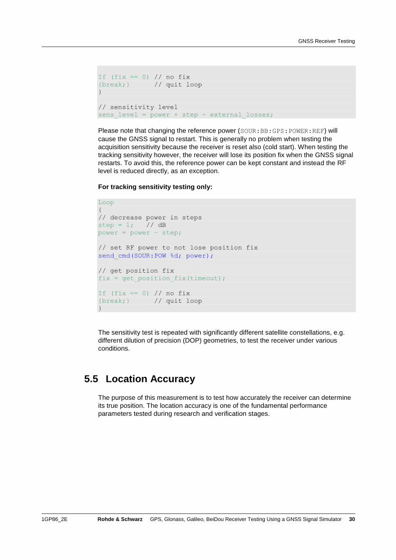
Please note that changing the reference power (SOUR:BB:GPS:POWER:REF) will
cause the GNSS signal to restart. This is generally no problem when testing the
acquisition sensitivity because the receiver is reset also (cold start). When testing the
tracking sensitivity however, the receiver will lose its position fix when the GNSS signal
restarts. To avoid this, the reference power can be kept constant and instead the RF
level is reduced directly, as an exception.
For tracking sensitivity testing only:
Loop
{
// decrease power in steps
step = 1; // dB
power = power – step;
// set RF power to not lose position fix
send_cmd(SOUR:POW %d; power);
// get position fix
fix = get_position_fix(timeout);
If (fix == 0) // no fix
{break;} // quit loop
}
The sensitivity test is repeated with significantly different satellite constellations, e.g.
different dilution of precision (DOP) geometries, to test the receiver under various
conditions.
5.5 Location Accuracy
The purpose of this measurement is to test how accurately the receiver can determine
its true position. The location accuracy is one of the fundamental performance
parameters tested during research and verification stages.
GNSS Receiver Testing
1GP86_2E Rohde & Schwarz GPS, Glonass, Galileo, BeiDou Receiver Testing Using a GNSS Signal Simulator 31
5.5.1 Static Location Accuracy
For this test, the SMBV simulates a realistic satellite constellation for a user-defined
location. The best simulation mode is “Auto Localization”, because in this mode the
SMBV automatically simulates the satellites that offer the best constellation for the set
location. If the user wishes to have full control over the simulated satellites, the “User
Localization” simulation mode can also be used. The SMBV comes with several
almanac files to choose from, but the user can also use up-to-date almanac files
available for download on the Internet.
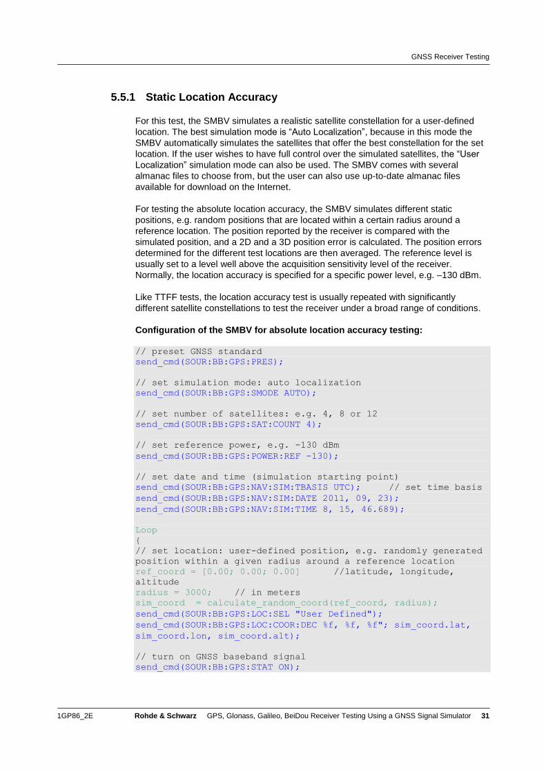
For testing the absolute location accuracy, the SMBV simulates different static
positions, e.g. random positions that are located within a certain radius around a
reference location. The position reported by the receiver is compared with the
simulated position, and a 2D and a 3D position error is calculated. The position errors
determined for the different test locations are then averaged. The reference level is
usually set to a level well above the acquisition sensitivity level of the receiver.
Normally, the location accuracy is specified for a specific power level, e.g. –130 dBm.
Like TTFF tests, the location accuracy test is usually repeated with significantly
different satellite constellations to test the receiver under a broad range of conditions.
Configuration of the SMBV for absolute location accuracy testing:
// preset GNSS standard
send_cmd(SOUR:BB:GPS:PRES);
// set simulation mode: auto localization
send_cmd(SOUR:BB:GPS:SMODE AUTO);
// set number of satellites: e.g. 4, 8 or 12
send_cmd(SOUR:BB:GPS:SAT:COUNT 4);
// set reference power, e.g. -130 dBm
send_cmd(SOUR:BB:GPS:POWER:REF -130);
// set date and time (simulation starting point)
send_cmd(SOUR:BB:GPS:NAV:SIM:TBASIS UTC); // set time basis
send_cmd(SOUR:BB:GPS:NAV:SIM:DATE 2011, 09, 23);
send_cmd(SOUR:BB:GPS:NAV:SIM:TIME 8, 15, 46.689);
Loop
{
// set location: user-defined position, e.g. randomly generated
position within a given radius around a reference location
ref_coord = [0.00; 0.00; 0.00] //latitude, longitude,
altitude
radius = 3000; // in meters
sim_coord = calculate_random_coord(ref_coord, radius);
send_cmd(SOUR:BB:GPS:LOC:SEL "User Defined");
send_cmd(SOUR:BB:GPS:LOC:COOR:DEC %f, %f, %f"; sim_coord.lat,
sim_coord.lon, sim_coord.alt);
// turn on GNSS baseband signal
send_cmd(SOUR:BB:GPS:STAT ON);
GNSS Receiver Testing
1GP86_2E Rohde & Schwarz GPS, Glonass, Galileo, BeiDou Receiver Testing Using a GNSS Signal Simulator 32
send_cmd(*OPC?); // synchronize
send_cmd(SOUR:BB:GPS:TRIG:EXEC); // trigger
// let the receiver acquire a 3D position fix
wait4fix();
// get position from receiver
meas_coord = get_position();
// calculate position error
position_error = calc_position_error(sim_coord, meas_coord);
}
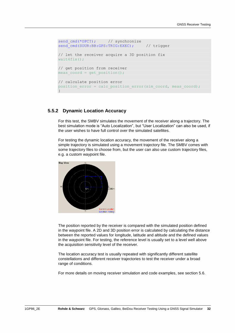
5.5.2 Dynamic Location Accuracy
For this test, the SMBV simulates the movement of the receiver along a trajectory. The
best simulation mode is “Auto Localization”, but “User Localization” can also be used, if
the user wishes to have full control over the simulated satellites.
For testing the dynamic location accuracy, the movement of the receiver along a
simple trajectory is simulated using a movement trajectory file. The SMBV comes with
some trajectory files to choose from, but the user can also use custom trajectory files,
e.g. a custom waypoint file.
The position reported by the receiver is compared with the simulated position defined
in the waypoint file. A 2D and 3D position error is calculated by calculating the distance
between the reported values for longitude, latitude and altitude and the defined values
in the waypoint file. For testing, the reference level is usually set to a level well above
the acquisition sensitivity level of the receiver.
The location accuracy test is usually repeated with significantly different satellite
constellations and different receiver trajectories to test the receiver under a broad
range of conditions.
For more details on moving receiver simulation and code examples, see section 5.6.
GNSS Receiver Testing
1GP86_2E Rohde & Schwarz GPS, Glonass, Galileo, BeiDou Receiver Testing Using a GNSS Signal Simulator 33
5.6 Moving Receiver
The purpose of this measurement is to test how the receiver performs while it
undergoes movement in either or all of the three directions: latitude, longitude and
altitude. Usually fundamental performance parameters such as location accuracy and
reacquisition time are measured. The test primarily shows how well the receiver can
track satellites while moving
at diverse velocities
with different accelerations
along different trajectories with ideal or restricted satellite visibility
Every receiver has a limit on the velocity, acceleration and jerk5 that it can handle.
For this test, the SMBV simulates the movement of the receiver along a trajectory, i.e.
the SMBV not only simulates the satellite motion (as done for a static location) but
additionally emulates the receiver motion. As a consequence, the receiver will navigate
as if it were indeed physically moving. The simulated trajectory is defined via a
movement trajectory file. The SMBV comes with some trajectory files to choose from,
but the user can also use any custom trajectory file. A trajectory file can have the
following format:
waypoint file
script file
NMEA data file
KML data file
XTD data file
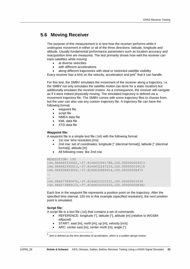
Waypoint file:
A waypoint file is a simple text file (.txt) with the following format:
1st row: time resolution [ms]
2nd row: set of coordinates: longitude [° (decimal format)], latitude [° (decimal
format)], altitude [m]
All following rows: like 2nd row
RESOLUTION: 150
144.966666334601,-37.8166633061788,100.000000009313
144.966662392613,-37.8166632247233,100.000000039116
144.966658453002,-37.8166630889914,100.00000008475
…
… 144.966677890476,-37.8166633333331,100.00000003539
144.966673889123,-37.8166633333333,100.000000008382
Each line in the waypoint file represents a position point on the trajectory. After the
specified time interval, 150 ms in this example (specified resolution), the next position
point is simulated.
Script file:
A script file is a text file (.txt) that contains a set of commands:
REFERENCE: longitude [°], latitude [°], altitude [m] (relative to WGS84
ellipsoid)
START: east [m], north [m], up [m], velocity [m/s]
ARC: center east [m], center north [m], angle [°]
5 Jerk is defined as the time derivative of acceleration, which is a sudden abrupt motion.
GNSS Receiver Testing
1GP86_2E Rohde & Schwarz GPS, Glonass, Galileo, BeiDou Receiver Testing Using a GNSS Signal Simulator 34
LINE: distance east [m], distance north [m], acceleration [m/s2]
STAY: time [ms]
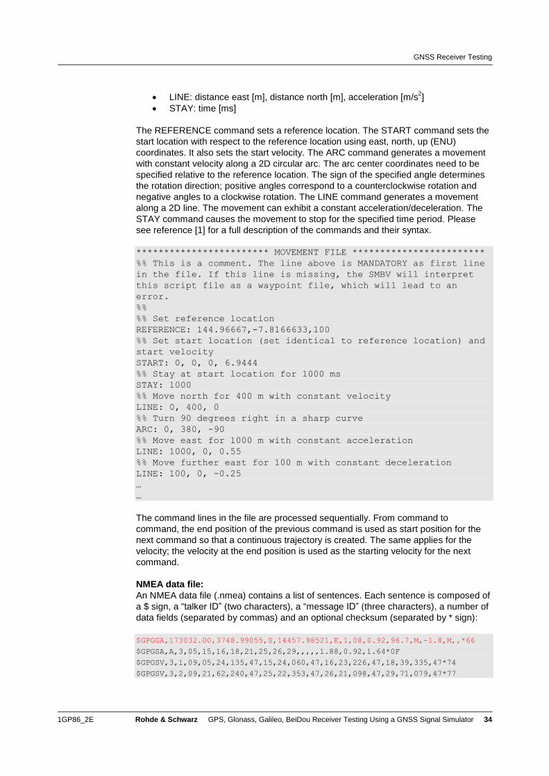
The REFERENCE command sets a reference location. The START command sets the
start location with respect to the reference location using east, north, up (ENU)
coordinates. It also sets the start velocity. The ARC command generates a movement
with constant velocity along a 2D circular arc. The arc center coordinates need to be
specified relative to the reference location. The sign of the specified angle determines
the rotation direction; positive angles correspond to a counterclockwise rotation and
negative angles to a clockwise rotation. The LINE command generates a movement
along a 2D line. The movement can exhibit a constant acceleration/deceleration. The
STAY command causes the movement to stop for the specified time period. Please
see reference [1] for a full description of the commands and their syntax.
************************ MOVEMENT FILE ************************
%% This is a comment. The line above is MANDATORY as first line
in the file. If this line is missing, the SMBV will interpret
this script file as a waypoint file, which will lead to an
error.
%%
%% Set reference location
REFERENCE: 144.96667,-7.8166633,100
%% Set start location (set identical to reference location) and
start velocity
START: 0, 0, 0, 6.9444
%% Stay at start location for 1000 ms
STAY: 1000
%% Move north for 400 m with constant velocity
LINE: 0, 400, 0
%% Turn 90 degrees right in a sharp curve
ARC: 0, 380, -90
%% Move east for 1000 m with constant acceleration
LINE: 1000, 0, 0.55
%% Move further east for 100 m with constant deceleration
LINE: 100, 0, -0.25
…
…
The command lines in the file are processed sequentially. From command to
command, the end position of the previous command is used as start position for the
next command so that a continuous trajectory is created. The same applies for the
velocity; the velocity at the end position is used as the starting velocity for the next
command.
NMEA data file:
An NMEA data file (.nmea) contains a list of sentences. Each sentence is composed of
a $ sign, a “talker ID” (two characters), a “message ID” (three characters), a number of
data fields (separated by commas) and an optional checksum (separated by * sign):
$GPGGA,173032.00,3748.99055,S,14457.98521,E,1,08,0.92,96.7,M,-1.8,M,,*66
$GPGSA,A,3,05,15,16,18,21,25,26,29,,,,,1.88,0.92,1.64*0F
$GPGSV,3,1,09,05,24,135,47,15,24,060,47,16,23,226,47,18,39,335,47*74
$GPGSV,3,2,09,21,62,240,47,25,22,353,47,26,21,098,47,29,71,079,47*77
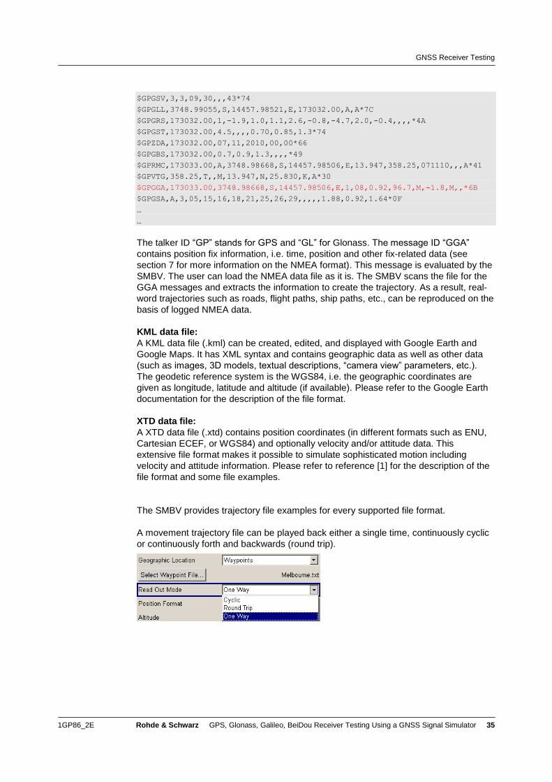
GNSS Receiver Testing
1GP86_2E Rohde & Schwarz GPS, Glonass, Galileo, BeiDou Receiver Testing Using a GNSS Signal Simulator 35
$GPGSV,3,3,09,30,,,43*74
$GPGLL,3748.99055,S,14457.98521,E,173032.00,A,A*7C
$GPGRS,173032.00,1,-1.9,1.0,1.1,2.6,-0.8,-4.7,2.0,-0.4,,,,*4A
$GPGST,173032.00,4.5,,,,0.70,0.85,1.3*74
$GPZDA,173032.00,07,11,2010,00,00*66
$GPGBS,173032.00,0.7,0.9,1.3,,,,*49
$GPRMC,173033.00,A,3748.98668,S,14457.98506,E,13.947,358.25,071110,,,A*41
$GPVTG,358.25,T,,M,13.947,N,25.830,K,A*30
$GPGGA,173033.00,3748.98668,S,14457.98506,E,1,08,0.92,96.7,M,-1.8,M,,*6B
$GPGSA,A,3,05,15,16,18,21,25,26,29,,,,,1.88,0.92,1.64*0F
…
…
The talker ID “GP” stands for GPS and “GL” for Glonass. The message ID “GGA”
contains position fix information, i.e. time, position and other fix-related data (see
section 7 for more information on the NMEA format). This message is evaluated by the
SMBV. The user can load the NMEA data file as it is. The SMBV scans the file for the
GGA messages and extracts the information to create the trajectory. As a result, real-
word trajectories such as roads, flight paths, ship paths, etc., can be reproduced on the
basis of logged NMEA data.
KML data file:
A KML data file (.kml) can be created, edited, and displayed with Google Earth and
Google Maps. It has XML syntax and contains geographic data as well as other data
(such as images, 3D models, textual descriptions, “camera view” parameters, etc.).
The geodetic reference system is the WGS84, i.e. the geographic coordinates are
given as longitude, latitude and altitude (if available). Please refer to the Google Earth
documentation for the description of the file format.
XTD data file:
A XTD data file (.xtd) contains position coordinates (in different formats such as ENU,
Cartesian ECEF, or WGS84) and optionally velocity and/or attitude data. This
extensive file format makes it possible to simulate sophisticated motion including
velocity and attitude information. Please refer to reference [1] for the description of the
file format and some file examples.
The SMBV provides trajectory file examples for every supported file format.
A movement trajectory file can be played back either a single time, continuously cyclic
or continuously forth and backwards (round trip).
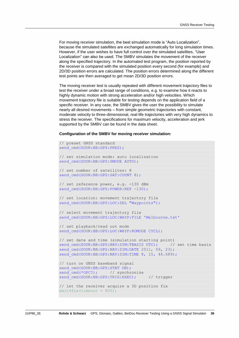
GNSS Receiver Testing
1GP86_2E Rohde & Schwarz GPS, Glonass, Galileo, BeiDou Receiver Testing Using a GNSS Signal Simulator 36
For moving receiver simulation, the best simulation mode is “Auto Localization”,
because the simulated satellites are exchanged automatically for long simulation times.
However, if the user wishes to have full control over the simulated satellites, “User
Localization” can also be used. The SMBV simulates the movement of the receiver
along the specified trajectory. In the automated test program, the position reported by
the receiver is compared with the simulated position every second (for example) and
2D/3D position errors are calculated. The position errors determined along the different
test points are then averaged to get mean 2D/3D position errors.
The moving receiver test is usually repeated with different movement trajectory files to
test the receiver under a broad range of conditions, e.g. to examine how it reacts to
highly dynamic motion with strong acceleration and/or high velocities. Which
movement trajectory file is suitable for testing depends on the application field of a
specific receiver. In any case, the SMBV gives the user the possibility to simulate
nearly all desired movements – from simple geometric trajectories with constant,
moderate velocity to three-dimensional, real-life trajectories with very high dynamics to
stress the receiver. The specifications for maximum velocity, acceleration and jerk
supported by the SMBV can be found in the data sheet.
Configuration of the SMBV for moving receiver simulation:
// preset GNSS standard
send_cmd(SOUR:BB:GPS:PRES);
// set simulation mode: auto localization
send_cmd(SOUR:BB:GPS:SMODE AUTO);
// set number of satellites: 8
send_cmd(SOUR:BB:GPS:SAT:COUNT 8);
// set reference power, e.g. -130 dBm
send_cmd(SOUR:BB:GPS:POWER:REF -130);
// set location: movement trajectory file
send_cmd(SOUR:BB:GPS:LOC:SEL "Waypoints");
// select movement trajectory file
send_cmd(SOUR:BB:GPS:LOC:WAYP:FILE 'Melbourne.txt'
// set playback/read out mode
send_cmd(SOUR:BB:GPS:LOC:WAYP:ROMODE CYCL);
// set date and time (simulation starting point)
send_cmd(SOUR:BB:GPS:NAV:SIM:TBASIS UTC); // set time basis
send_cmd(SOUR:BB:GPS:NAV:SIM:DATE 2011, 09, 23);
send_cmd(SOUR:BB:GPS:NAV:SIM:TIME 8, 15, 46.689);
// turn on GNSS baseband signal
send_cmd(SOUR:BB:GPS:STAT ON);
send_cmd(*OPC?); // synchronize
send_cmd(SOUR:BB:GPS:TRIG:EXEC); // trigger
// let the receiver acquire a 3D position fix
wait4fix(timeout = 800);
GNSS Receiver Testing
1GP86_2E Rohde & Schwarz GPS, Glonass, Galileo, BeiDou Receiver Testing Using a GNSS Signal Simulator 37
Loop
{
// get position and time from receiver
meas_coord = get_position();
meas_time = get_time();
// query SMBV for simulated position at time point reported by
receiver
sim_coord = send_cmd(SOUR:BB:GPS:RT:RLOC:COOR:DEC? UTC, %f, %f,
%f, %f, %f, %f; meas_time.year, meas_time.month, meas_time.day,
meas_time.hour, meas_time.min, meas_time.sec);
// calculate position error
position_error = calc_position_error(meas_coord, sim_coord)
// wait 1 second
wait(1);
count = count + 1;
// quit loop, e.g. after 500 iterations
If (count == 500)
{break;}
} Hint: Typically, the TTFF is shorter if the receiver is stationary and not moving. It thus makes sense to remain a while at the start position before actually starting the movement in order to enable the receiver to acquire a position fix more rapidly. The “parking” must be included in the movement trajectory file. Note that the SMBV supports two kinds of receiver movement simulation:
Using predetermined trajectories from files such as waypoint, NMEA data, etc. as described above.
Using remote control to dictate the trajectory in realtime as used in hardware in the loop (HIL) setups. Please see reference [8] for a detailed description of how to operate the SMBV in HIL applications.
5.7 Long-Term Experiment
The purpose of this measurement is to test how reliably the receiver can deliver valid
and precise position fixes over a long test period. Such long-term tests run for at least
24 hours but can also last as long as two full days or even more.
GNSS Receiver Testing
1GP86_2E Rohde & Schwarz GPS, Glonass, Galileo, BeiDou Receiver Testing Using a GNSS Signal Simulator 38
For this test, the SMBV simulates a realistic satellite constellation for a static or moving
receiver. The “Auto Localization” simulation mode is used, because in this mode the
SMBV automatically simulates the satellites that offer the best constellation. As the
simulated satellites move in the sky as real satellites do, there is a steady restructuring
of visible satellites. While some satellites move across the sky and finally vanish
beyond the horizon, other satellites appear on the horizon. The SMBV is able to
simulate this situation by automatically exchanging the satellite signals in realtime. The
simulation time is thus unlimited, which makes the SMBV ideal for long-term testing.
For example, the number of simulated satellites is set to “6”. The SMBV will then
simulate the six satellites that offer the best constellation (best DOP), e.g. SV-IDs 3,
11, 14, 18, 23, 25. If one satellite gets close to the horizon, it is automatically replaced
by a new one, e.g. SV-ID 25 is replaced by SV-ID 15. Over the day, the SMBV thus
simulates all SV-IDs as the satellites rotate across the sky.
During the test period, the receiver’s performance is constantly monitored. Of special
interest is the overall time period during which the receiver delivered a valid position
fix. Also the average location accuracy is of interest.
Configuration of the SMBV for a long-term experiment:
// preset GNSS standard
send_cmd(SOUR:BB:GPS:PRES);
// set simulation mode: auto localization
send_cmd(SOUR:BB:GPS:SMODE AUTO);
// Optional: select almanac file
// up-to-date almanac files are available on the Internet.
send_cmd(SOUR:BB:GPS:NAV:ALM:GPS:FILE 'GPS_SEM585.txt');
// set number of satellites: 6
send_cmd(SOUR:BB:GPS:SAT:COUNT 6);
// set reference power, e.g. -130 dBm
send_cmd(SOUR:BB:GPS:POWER:REF -130);
if (moving_receiver == true)
{
// set location: movement trajectory file
send_cmd(SOUR:BB:GPS:LOC:SEL "Waypoints");
// select movement trajectory file
send_cmd(SOUR:BB:GPS:LOC:WAYP:FILE 'Melbourne.txt'
// set playback/read out mode
send_cmd(SOUR:BB:GPS:LOC:WAYP:ROMODE CYCL);
}
else // static receiver
{
// set location: user location
send_cmd(SOUR:BB:GPS:LOC:SEL "User Defined");
// set position coordinates
send_cmd(SOUR:BB:GPS:LOC:COOR:DEC 90, 180, 5.5);
}
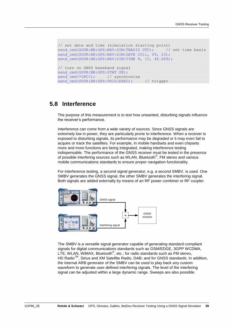
GNSS Receiver Testing
1GP86_2E Rohde & Schwarz GPS, Glonass, Galileo, BeiDou Receiver Testing Using a GNSS Signal Simulator 39
// set date and time (simulation starting point)
send_cmd(SOUR:BB:GPS:NAV:SIM:TBASIS UTC); // set time basis
send_cmd(SOUR:BB:GPS:NAV:SIM:DATE 2011, 09, 23);
send_cmd(SOUR:BB:GPS:NAV:SIM:TIME 8, 15, 46.689);
// turn on GNSS baseband signal
send_cmd(SOUR:BB:GPS:STAT ON);
send_cmd(*OPC?); // synchronize
send_cmd(SOUR:BB:GPS:TRIG:EXEC); // trigger
5.8 Interference
The purpose of this measurement is to test how unwanted, disturbing signals influence
the receiver’s performance.
Interference can come from a wide variety of sources. Since GNSS signals are
extremely low in power, they are particularly prone to interference. When a receiver is
exposed to disturbing signals, its performance may be degraded or it may even fail to
acquire or track the satellites. For example, in mobile handsets and even chipsets
more and more functions are being integrated, making interference testing
indispensable. The performance of the GNSS receiver must be tested in the presence
of possible interfering sources such as WLAN, Bluetooth®, FM stereo and various
mobile communications standards to ensure proper navigation functionality.
For interference testing, a second signal generator, e.g. a second SMBV, is used. One
SMBV generates the GNSS signal, the other SMBV generates the interfering signal.
Both signals are added externally by means of an RF power combiner or RF coupler.
GNSS
receiver
GNSS signal
Interfering signal
+
The SMBV is a versatile signal generator capable of generating standard-compliant
signals for digital communications standards such as GSM/EDGE, 3GPP WCDMA,
LTE, WLAN, WiMAX, Bluetooth®, etc.; for radio standards such as FM stereo,
HD RadioTM
, Sirius and XM Satellite Radio, DAB; and for GNSS standards. In addition,
the internal ARB generator of the SMBV can be used to play back any custom
waveform to generate user-defined interfering signals. The level of the interfering
signal can be adjusted within a large dynamic range. Sweeps are also possible.
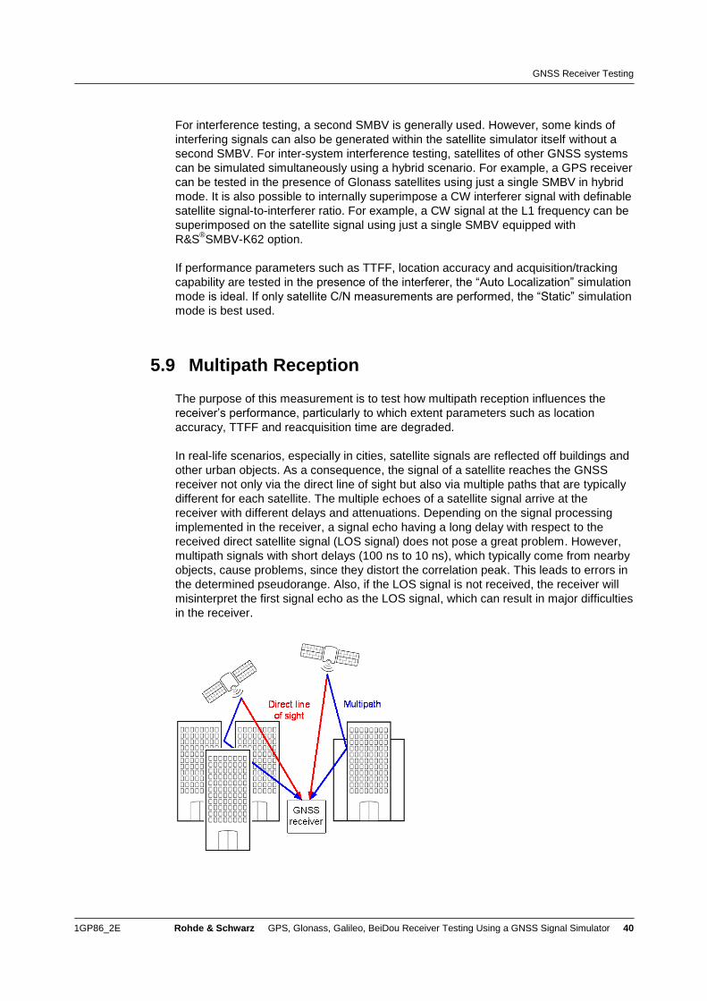
GNSS Receiver Testing
1GP86_2E Rohde & Schwarz GPS, Glonass, Galileo, BeiDou Receiver Testing Using a GNSS Signal Simulator 40
For interference testing, a second SMBV is generally used. However, some kinds of
interfering signals can also be generated within the satellite simulator itself without a
second SMBV. For inter-system interference testing, satellites of other GNSS systems
can be simulated simultaneously using a hybrid scenario. For example, a GPS receiver
can be tested in the presence of Glonass satellites using just a single SMBV in hybrid
mode. It is also possible to internally superimpose a CW interferer signal with definable
satellite signal-to-interferer ratio. For example, a CW signal at the L1 frequency can be
superimposed on the satellite signal using just a single SMBV equipped with
R&S®SMBV-K62 option.
If performance parameters such as TTFF, location accuracy and acquisition/tracking
capability are tested in the presence of the interferer, the “Auto Localization” simulation
mode is ideal. If only satellite C/N measurements are performed, the “Static” simulation
mode is best used.
5.9 Multipath Reception
The purpose of this measurement is to test how multipath reception influences the
receiver’s performance, particularly to which extent parameters such as location
accuracy, TTFF and reacquisition time are degraded.
In real-life scenarios, especially in cities, satellite signals are reflected off buildings and
other urban objects. As a consequence, the signal of a satellite reaches the GNSS
receiver not only via the direct line of sight but also via multiple paths that are typically
different for each satellite. The multiple echoes of a satellite signal arrive at the
receiver with different delays and attenuations. Depending on the signal processing
implemented in the receiver, a signal echo having a long delay with respect to the
received direct satellite signal (LOS signal) does not pose a great problem. However,
multipath signals with short delays (100 ns to 10 ns), which typically come from nearby
objects, cause problems, since they distort the correlation peak. This leads to errors in
the determined pseudorange. Also, if the LOS signal is not received, the receiver will
misinterpret the first signal echo as the LOS signal, which can result in major difficulties
in the receiver.
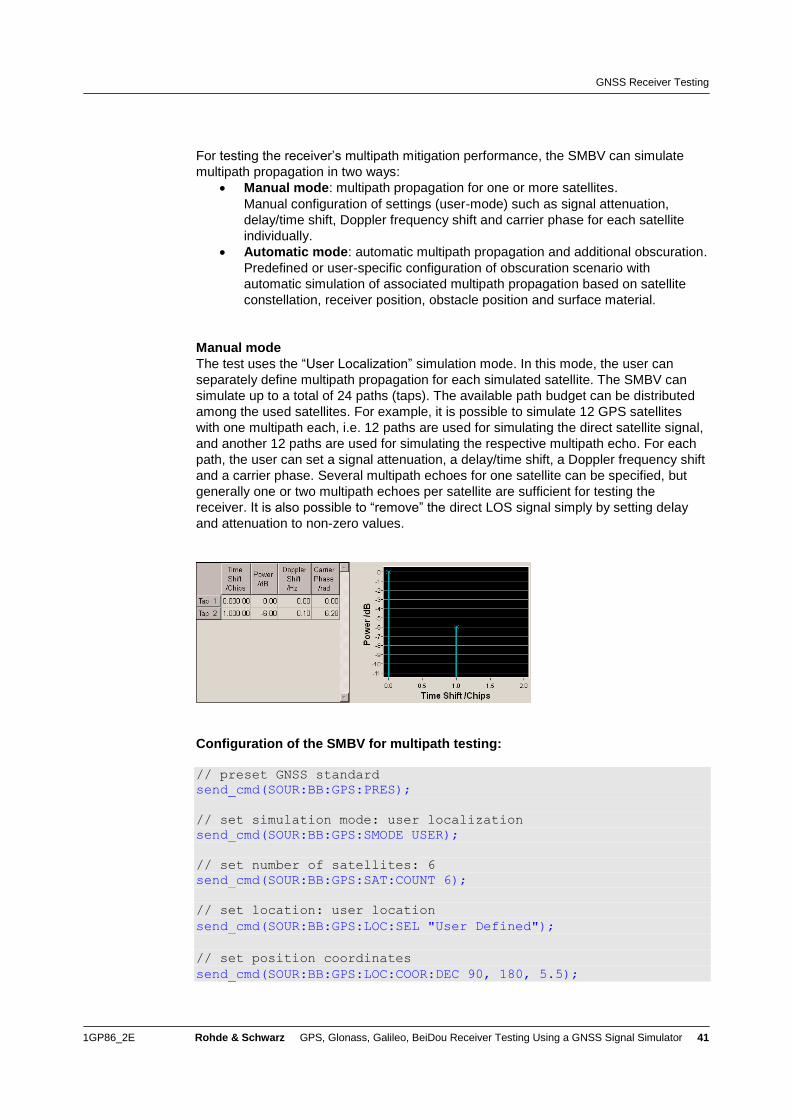
GNSS Receiver Testing
1GP86_2E Rohde & Schwarz GPS, Glonass, Galileo, BeiDou Receiver Testing Using a GNSS Signal Simulator 41
For testing the receiver’s multipath mitigation performance, the SMBV can simulate
multipath propagation in two ways:
Manual mode: multipath propagation for one or more satellites.
Manual configuration of settings (user-mode) such as signal attenuation,
delay/time shift, Doppler frequency shift and carrier phase for each satellite
individually.
Automatic mode: automatic multipath propagation and additional obscuration.
Predefined or user-specific configuration of obscuration scenario with
automatic simulation of associated multipath propagation based on satellite
constellation, receiver position, obstacle position and surface material.
Manual mode
The test uses the “User Localization” simulation mode. In this mode, the user can
separately define multipath propagation for each simulated satellite. The SMBV can
simulate up to a total of 24 paths (taps). The available path budget can be distributed
among the used satellites. For example, it is possible to simulate 12 GPS satellites
with one multipath each, i.e. 12 paths are used for simulating the direct satellite signal,
and another 12 paths are used for simulating the respective multipath echo. For each
path, the user can set a signal attenuation, a delay/time shift, a Doppler frequency shift
and a carrier phase. Several multipath echoes for one satellite can be specified, but
generally one or two multipath echoes per satellite are sufficient for testing the
receiver. It is also possible to “remove” the direct LOS signal simply by setting delay
and attenuation to non-zero values.
Configuration of the SMBV for multipath testing:
// preset GNSS standard
send_cmd(SOUR:BB:GPS:PRES);
// set simulation mode: user localization
send_cmd(SOUR:BB:GPS:SMODE USER);
// set number of satellites: 6
send_cmd(SOUR:BB:GPS:SAT:COUNT 6);
// set location: user location
send_cmd(SOUR:BB:GPS:LOC:SEL "User Defined");
// set position coordinates
send_cmd(SOUR:BB:GPS:LOC:COOR:DEC 90, 180, 5.5);
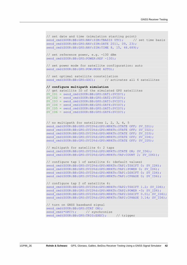
GNSS Receiver Testing
1GP86_2E Rohde & Schwarz GPS, Glonass, Galileo, BeiDou Receiver Testing Using a GNSS Signal Simulator 42
// set date and time (simulation starting point)
send_cmd(SOUR:BB:GPS:NAV:SIM:TBASIS UTC); // set time basis
send_cmd(SOUR:BB:GPS:NAV:SIM:DATE 2011, 09, 23);
send_cmd(SOUR:BB:GPS:NAV:SIM:TIME 8, 15, 46.689);
// set reference power, e.g. -130 dBm
send_cmd(SOUR:BB:GPS:POWER:REF -130);
// set power mode for satellite configuration: auto
send_cmd(SOUR:BB:GPS:POW:MODE AUTO);
// set optimal satellite constellation
send_cmd(SOUR:BB:GPS:GOC); // activates all 6 satellites
// configure multipath simulation
// get satellite ID of the simulated GPS satellites
SV_ID1 = send_cmd(SOUR:BB:GPS:SAT1:SVID?);
SV_ID2 = send_cmd(SOUR:BB:GPS:SAT2:SVID?);
SV_ID3 = send_cmd(SOUR:BB:GPS:SAT3:SVID?);
SV_ID4 = send_cmd(SOUR:BB:GPS:SAT4:SVID?);
SV_ID5 = send_cmd(SOUR:BB:GPS:SAT5:SVID?);
SV_ID6 = send_cmd(SOUR:BB:GPS:SAT6:SVID?);
// no multipath for satellites 1, 2, 3, 4, 5
send_cmd(SOUR:BB:GPS:SVID%d:GPS:MPATh:STATE OFF; SV_ID1);
send_cmd(SOUR:BB:GPS:SVID%d:GPS:MPATh:STATE OFF; SV_ID2);
send_cmd(SOUR:BB:GPS:SVID%d:GPS:MPATh:STATE OFF; SV_ID3);
send_cmd(SOUR:BB:GPS:SVID%d:GPS:MPATh:STATE OFF; SV_ID4);
send_cmd(SOUR:BB:GPS:SVID%d:GPS:MPATh:STATE OFF; SV_ID5);
// multipath for satellite 6: 2 taps
send_cmd(SOUR:BB:GPS:SVID%d:GPS:MPATh:STATE ON; SV_ID6);
send_cmd(SOUR:BB:GPS:SVID%d:GPS:MPATh:TAP:COUNT 2; SV_ID6));
// configure tap 1 of satellite 6: (default values)
send_cmd(SOUR:BB:GPS:SVID%d:GPS:MPATh:TAP1:TSHIFT 0; SV_ID6);
send_cmd(SOUR:BB:GPS:SVID%d:GPS:MPATh:TAP1:POWER 0; SV_ID6);
send_cmd(SOUR:BB:GPS:SVID%d:GPS:MPATh:TAP1:DSHIFT 0; SV_ID6);
send_cmd(SOUR:BB:GPS:SVID%d:GPS:MPATh:TAP1:CPHASE 0; SV_ID6);
// configure tap 2 of satellite 6:
send_cmd(SOUR:BB:GPS:SVID%d:GPS:MPATh:TAP2:TSHIFT 1.2; SV_ID6);
send_cmd(SOUR:BB:GPS:SVID%d:GPS:MPATh:TAP2:POWER -3; SV_ID6);
send_cmd(SOUR:BB:GPS:SVID%d:GPS:MPATh:TAP2:DSHIFT 0.01; SV_ID6);
send_cmd(SOUR:BB:GPS:SVID%d:GPS:MPATh:TAP2:CPHASE 3.14; SV_ID6);
// turn on GNSS baseband signal
send_cmd(SOUR:BB:GPS:STAT ON);
send_cmd(*OPC?); // synchronize
send_cmd(SOUR:BB:GPS:TRIG:EXEC); // trigger
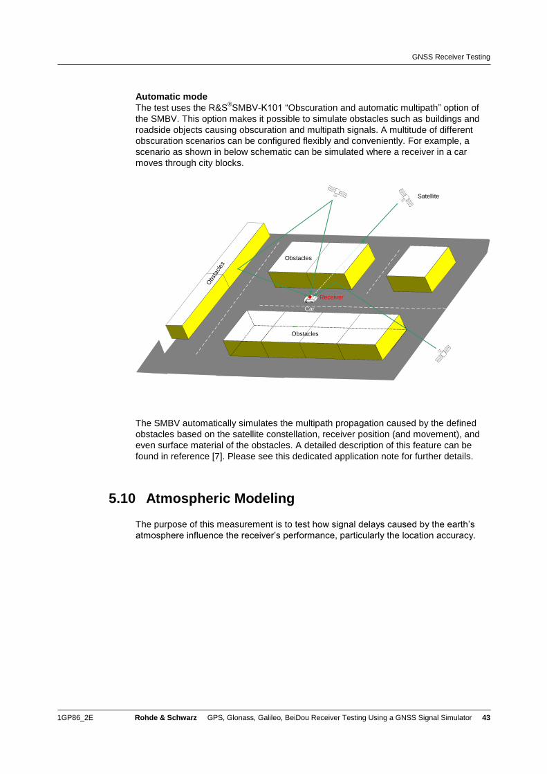
GNSS Receiver Testing
1GP86_2E Rohde & Schwarz GPS, Glonass, Galileo, BeiDou Receiver Testing Using a GNSS Signal Simulator 43
Automatic mode
The test uses the R&S®SMBV-K101 “Obscuration and automatic multipath” option of
the SMBV. This option makes it possible to simulate obstacles such as buildings and
roadside objects causing obscuration and multipath signals. A multitude of different
obscuration scenarios can be configured flexibly and conveniently. For example, a
scenario as shown in below schematic can be simulated where a receiver in a car
moves through city blocks.
Receiver
Obstacles
Car
Obstacles
Obs
tacl
es
Satellite
The SMBV automatically simulates the multipath propagation caused by the defined
obstacles based on the satellite constellation, receiver position (and movement), and
even surface material of the obstacles. A detailed description of this feature can be
found in reference [7]. Please see this dedicated application note for further details.
5.10 Atmospheric Modeling
The purpose of this measurement is to test how signal delays caused by the earth’s
atmosphere influence the receiver’s performance, particularly the location accuracy.
GNSS Receiver Testing
1GP86_2E Rohde & Schwarz GPS, Glonass, Galileo, BeiDou Receiver Testing Using a GNSS Signal Simulator 44
On their way from the satellites to the receiver, the GNSS signals travel through the
earth’s atmosphere, which is composed of different layers. Two of these layers that
play a role for GNSS are the ionosphere and the troposphere. The ionosphere is a
layer of ionized gas in the upper atmosphere that influences radio wave propagation
due to its dispersive nature. The troposphere forms the lowest atmospheric layer – the
“weather layer” – and is a non-dispersive medium. A GNSS signal is assumed to travel
at the speed of light (true in space vacuum). However, the troposphere and mostly the
ionosphere refract and slow down the signal, thus causing a delay in the signal that
leads to an error in the receiver’s position fix. To minimize the error induced by the
ionosphere, the atmospheric conditions are mathematically modeled, i.e. one tries to
predict the delay. The up-to-date prediction of the ionospheric delay is broadcasted via
the navigation message of every satellite. The receiver can use this information to
compensate for this delay and reduce the error in the position fix. Mathematical
modeling is also used to predict tropospheric delays, but these predictions are not
broadcasted via the navigation message, since tropospheric conditions are very
regional. In addition, this modeling of a “standard atmosphere” yields a good estimation
for the tropospheric delays (for elevations > 5°).
The SMBV can simulate the propagation characteristics of the satellite signals in the
ionosphere and the troposphere using the appropriate models. For GPS, the Klobuchar
model is used as ionospheric model. The user can set the 8 Klobuchar coefficients 0
to 3 and 0 to 3. These coefficients are used for simulating the ionospheric delay
and are included in the navigation message of the simulated satellites. If ionospheric
modeling is disabled, the set coefficients are nevertheless included in the navigation
message generated by the SMBV. Note that setting the 8 Klobuchar coefficients to
zero is not equivalent to disabling ionospheric modeling. The STANAG model is used
as tropospheric model.
Configuration of the SMBV for simulating atmospheric conditions:
// GPS
// set ionospheric model to activate ionospheric modeling
send_cmd(SOUR:BB:GPS:ATM:GPS:ION:MODel KLOBuchar);
// set Klobuchar coefficients
send_cmd(SOUR:BB:GPS:ATM:GPS:ION:ALPHa0 5);
send_cmd(SOUR:BB:GPS:ATM:GPS:ION:ALPHa1 2);
send_cmd(SOUR:BB:GPS:ATM:GPS:ION:ALPHa2 -1);
send_cmd(SOUR:BB:GPS:ATM:GPS:ION:ALPHa3 -1);
send_cmd(SOUR:BB:GPS:ATM:GPS:ION:BETA0 39);
send_cmd(SOUR:BB:GPS:ATM:GPS:ION:BETA1 4);
send_cmd(SOUR:BB:GPS:ATM:GPS:ION:BETA2 -1);
send_cmd(SOUR:BB:GPS:ATM:GPS:ION:BETA3 -6);
// set tropospheric model to activate tropospheric modeling
send_cmd(SOUR:BB:GPS:ATM:GPS:TROP:MODel STANAG);
// atmospheric modeling can be disabled with
// send_cmd(SOUR:BB:GPS:ATM:GPS:ION:MODel NONE);
// send_cmd(SOUR:BB:GPS:ATM:GPS:TROP:MODel NONE);
// note: the set Klobuchar coefficients are still transmitted
via the navigation message of the simulated satellites, even if
ionospheric modeling is turned off
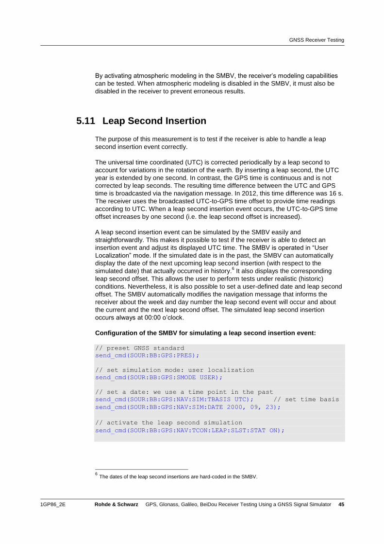
GNSS Receiver Testing
1GP86_2E Rohde & Schwarz GPS, Glonass, Galileo, BeiDou Receiver Testing Using a GNSS Signal Simulator 45
By activating atmospheric modeling in the SMBV, the receiver’s modeling capabilities
can be tested. When atmospheric modeling is disabled in the SMBV, it must also be
disabled in the receiver to prevent erroneous results.
5.11 Leap Second Insertion
The purpose of this measurement is to test if the receiver is able to handle a leap
second insertion event correctly.
The universal time coordinated (UTC) is corrected periodically by a leap second to
account for variations in the rotation of the earth. By inserting a leap second, the UTC
year is extended by one second. In contrast, the GPS time is continuous and is not
corrected by leap seconds. The resulting time difference between the UTC and GPS
time is broadcasted via the navigation message. In 2012, this time difference was 16 s.
The receiver uses the broadcasted UTC-to-GPS time offset to provide time readings
according to UTC. When a leap second insertion event occurs, the UTC-to-GPS time
offset increases by one second (i.e. the leap second offset is increased).
A leap second insertion event can be simulated by the SMBV easily and
straightforwardly. This makes it possible to test if the receiver is able to detect an
insertion event and adjust its displayed UTC time. The SMBV is operated in “User
Localization” mode. If the simulated date is in the past, the SMBV can automatically
display the date of the next upcoming leap second insertion (with respect to the
simulated date) that actually occurred in history.6 It also displays the corresponding
leap second offset. This allows the user to perform tests under realistic (historic)
conditions. Nevertheless, it is also possible to set a user-defined date and leap second
offset. The SMBV automatically modifies the navigation message that informs the
receiver about the week and day number the leap second event will occur and about
the current and the next leap second offset. The simulated leap second insertion
occurs always at 00:00 o’clock.
Configuration of the SMBV for simulating a leap second insertion event:
// preset GNSS standard
send_cmd(SOUR:BB:GPS:PRES);
// set simulation mode: user localization
send_cmd(SOUR:BB:GPS:SMODE USER);
// set a date: we use a time point in the past
send_cmd(SOUR:BB:GPS:NAV:SIM:TBASIS UTC); // set time basis
send_cmd(SOUR:BB:GPS:NAV:SIM:DATE 2000, 09, 23);
// activate the leap second simulation
send_cmd(SOUR:BB:GPS:NAV:TCON:LEAP:SLST:STAT ON);
6 The dates of the leap second insertions are hard-coded in the SMBV.
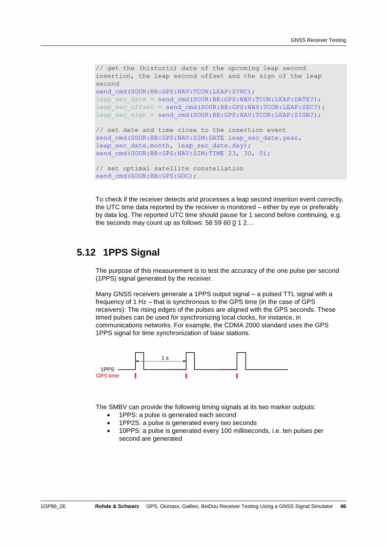
GNSS Receiver Testing
1GP86_2E Rohde & Schwarz GPS, Glonass, Galileo, BeiDou Receiver Testing Using a GNSS Signal Simulator 46
// get the (historic) date of the upcoming leap second
insertion, the leap second offset and the sign of the leap
second
send_cmd(SOUR:BB:GPS:NAV:TCON:LEAP:SYNC);
leap_sec_date = send_cmd(SOUR:BB:GPS:NAV:TCON:LEAP:DATE?);
leap_sec_offset = send_cmd(SOUR:BB:GPS:NAV:TCON:LEAP:SEC?);
leap_sec_sign = send_cmd(SOUR:BB:GPS:NAV:TCON:LEAP:SIGN?);
// set date and time close to the insertion event
send_cmd(SOUR:BB:GPS:NAV:SIM:DATE leap_sec_date.year,
leap_sec_date.month, leap_sec_date.day);
send_cmd(SOUR:BB:GPS:NAV:SIM:TIME 23, 30, 0);
// set optimal satellite constellation
send_cmd(SOUR:BB:GPS:GOC);
To check if the receiver detects and processes a leap second insertion event correctly,
the UTC time data reported by the receiver is monitored – either by eye or preferably
by data log. The reported UTC time should pause for 1 second before continuing, e.g.
the seconds may count up as follows: 58 59 60 0 1 2…
5.12 1PPS Signal
The purpose of this measurement is to test the accuracy of the one pulse per second
(1PPS) signal generated by the receiver.
Many GNSS receivers generate a 1PPS output signal – a pulsed TTL signal with a
frequency of 1 Hz – that is synchronous to the GPS time (in the case of GPS
receivers): The rising edges of the pulses are aligned with the GPS seconds. These
timed pulses can be used for synchronizing local clocks, for instance, in
communications networks. For example, the CDMA 2000 standard uses the GPS
1PPS signal for time synchronization of base stations.
1PPS
1 s
GPS time
The SMBV can provide the following timing signals at its two marker outputs:
1PPS: a pulse is generated each second
1PP2S: a pulse is generated every two seconds
10PPS: a pulse is generated every 100 milliseconds, i.e. ten pulses per
second are generated
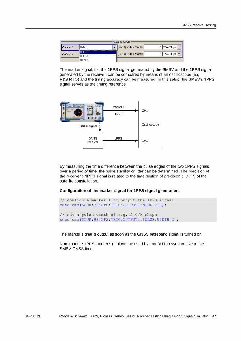
GNSS Receiver Testing
1GP86_2E Rohde & Schwarz GPS, Glonass, Galileo, BeiDou Receiver Testing Using a GNSS Signal Simulator 47
The marker signal, i.e. the 1PPS signal generated by the SMBV and the 1PPS signal
generated by the receiver, can be compared by means of an oscilloscope (e.g.
R&S RTO) and the timing accuracy can be measured. In this setup, the SMBV’s 1PPS
signal serves as the timing reference.
Marker 1
1PPS
GNSS
receiver
1PPS
Oscilloscope
CH1
CH2
GNSS signal
By measuring the time difference between the pulse edges of the two 1PPS signals
over a period of time, the pulse stability or jitter can be determined. The precision of
the receiver’s 1PPS signal is related to the time dilution of precision (TDOP) of the
satellite constellation.
Configuration of the marker signal for 1PPS signal generation:
// configure marker 1 to output the 1PPS signal
send_cmd(SOUR:BB:GPS:TRIG:OUTPUT1:MODE PPS);
// set a pulse width of e.g. 2 C/A chips
send_cmd(SOUR:BB:GPS:TRIG:OUTPUT1:PULSE:WIDTH 2);
The marker signal is output as soon as the GNSS baseband signal is turned on.
Note that the 1PPS marker signal can be used by any DUT to synchronize to the
SMBV GNSS time.
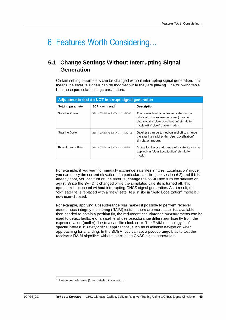
Features Worth Considering…
1GP86_2E Rohde & Schwarz GPS, Glonass, Galileo, BeiDou Receiver Testing Using a GNSS Signal Simulator 48
6 Features Worth Considering…
6.1 Change Settings Without Interrupting Signal
Generation
Certain setting parameters can be changed without interrupting signal generation. This
means the satellite signals can be modified while they are playing. The following table
lists these particular settings parameters.
Adjustments that do NOT interrupt signal generation
Setting parameter SCPI command7 Description
Satellite Power BB:<GNSS>:SAT<ch>:POW The power level of individual satellites (in
relation to the reference power) can be
changed (in “User Localization” simulation
mode with “User” power mode).
Satellite State BB:<GNSS>:SAT<ch>:STAT Satellites can be turned on and off to change
the satellite visibility (in “User Localization”
simulation mode).
Pseudorange Bias BB:<GNSS>:SAT<ch>:PRB A bias for the pseudorange of a satellite can be
applied (in “User Localization” simulation
mode).
For example, if you want to manually exchange satellites in “User Localization” mode, you can query the current elevation of a particular satellite (see section 6.2) and if it is already poor, you can turn off the satellite, change the SV-ID and turn the satellite on again. Since the SV-ID is changed while the simulated satellite is turned off, this operation is executed without interrupting GNSS signal generation. As a result, the “old” satellite is replaced with a “new” satellite just like in “Auto Localization” mode but now user-dictated. For example, applying a pseudorange bias makes it possible to perform receiver autonomous integrity monitoring (RAIM) tests. If there are more satellites available than needed to obtain a position fix, the redundant pseudorange measurements can be used to detect faults, e.g. a satellite whose pseudorange differs significantly from the expected value (outlier) due to a satellite clock error. The RAIM technology is of special interest in safety-critical applications, such as in aviation navigation when approaching for a landing. In the SMBV, you can set a pseudorange bias to test the receiver’s RAIM algorithm without interrupting GNSS signal generation.
7 Please see reference [1] for detailed information.
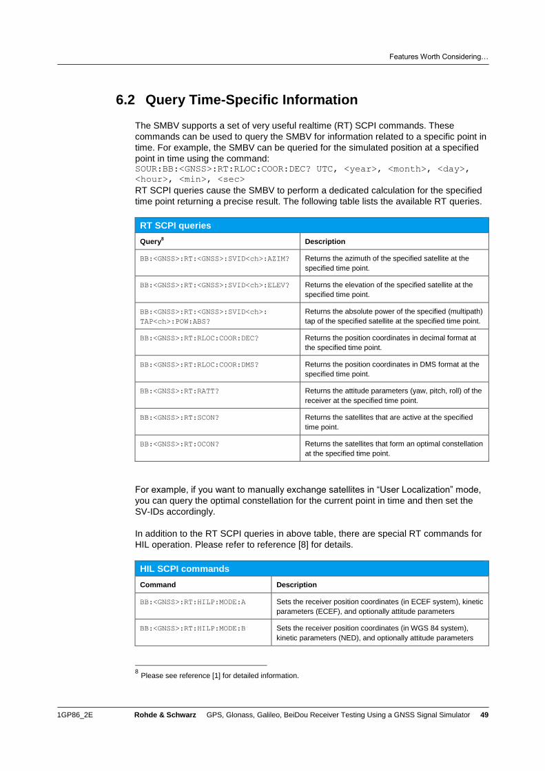
Features Worth Considering…
1GP86_2E Rohde & Schwarz GPS, Glonass, Galileo, BeiDou Receiver Testing Using a GNSS Signal Simulator 49
6.2 Query Time-Specific Information
The SMBV supports a set of very useful realtime (RT) SCPI commands. These
commands can be used to query the SMBV for information related to a specific point in
time. For example, the SMBV can be queried for the simulated position at a specified
point in time using the command: SOUR:BB:<GNSS>:RT:RLOC:COOR:DEC? UTC, <year>, <month>, <day>,
<hour>, <min>, <sec>
RT SCPI queries cause the SMBV to perform a dedicated calculation for the specified
time point returning a precise result. The following table lists the available RT queries.
RT SCPI queries
Query8 Description
BB:<GNSS>:RT:<GNSS>:SVID<ch>:AZIM? Returns the azimuth of the specified satellite at the
specified time point.
BB:<GNSS>:RT:<GNSS>:SVID<ch>:ELEV? Returns the elevation of the specified satellite at the
specified time point.
BB:<GNSS>:RT:<GNSS>:SVID<ch>:
TAP<ch>:POW:ABS?
Returns the absolute power of the specified (multipath)
tap of the specified satellite at the specified time point.
BB:<GNSS>:RT:RLOC:COOR:DEC? Returns the position coordinates in decimal format at
the specified time point.
BB:<GNSS>:RT:RLOC:COOR:DMS? Returns the position coordinates in DMS format at the
specified time point.
BB:<GNSS>:RT:RATT? Returns the attitude parameters (yaw, pitch, roll) of the
receiver at the specified time point.
BB:<GNSS>:RT:SCON? Returns the satellites that are active at the specified
time point.
BB:<GNSS>:RT:OCON? Returns the satellites that form an optimal constellation
at the specified time point.
For example, if you want to manually exchange satellites in “User Localization” mode,
you can query the optimal constellation for the current point in time and then set the
SV-IDs accordingly.
In addition to the RT SCPI queries in above table, there are special RT commands for
HIL operation. Please refer to reference [8] for details.
HIL SCPI commands
Command Description
BB:<GNSS>:RT:HILP:MODE:A Sets the receiver position coordinates (in ECEF system), kinetic
parameters (ECEF), and optionally attitude parameters
BB:<GNSS>:RT:HILP:MODE:B Sets the receiver position coordinates (in WGS 84 system),
kinetic parameters (NED), and optionally attitude parameters
8 Please see reference [1] for detailed information.
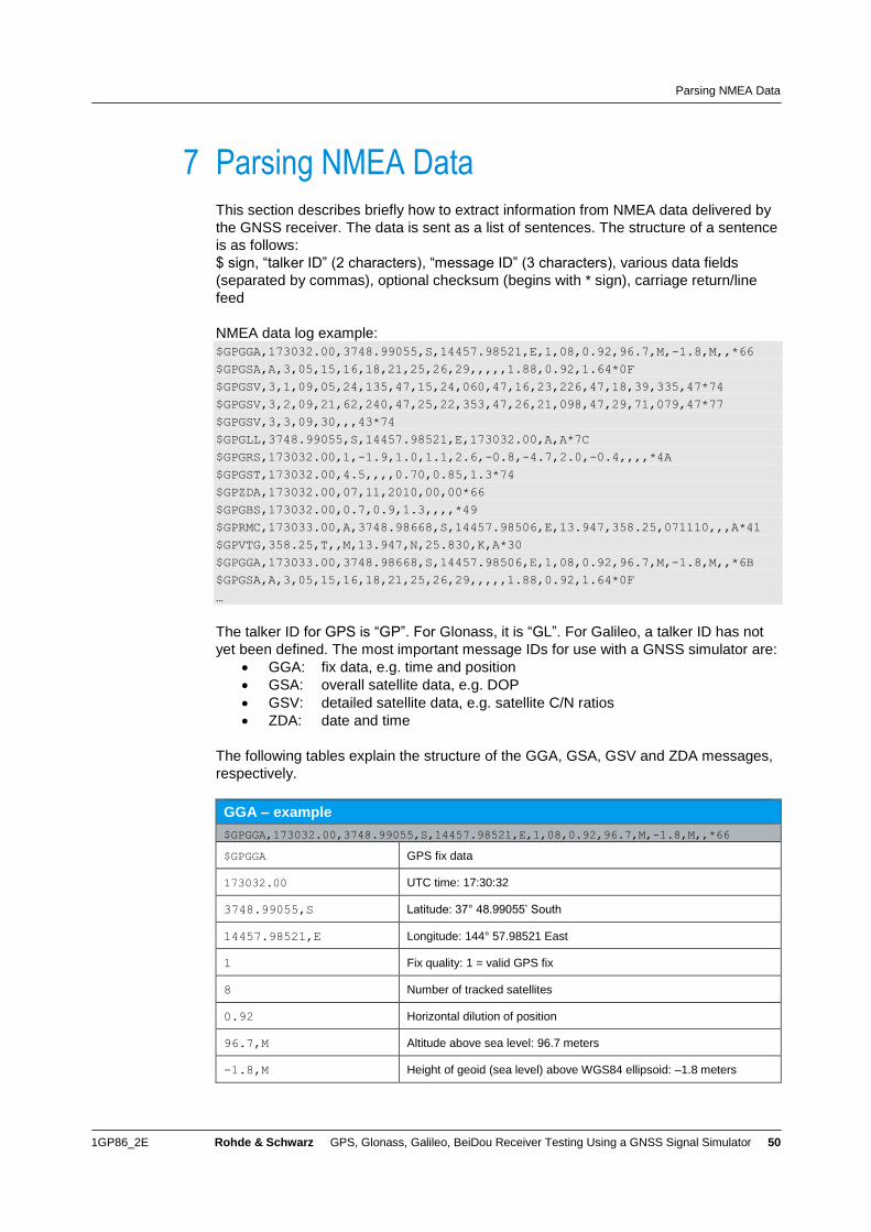
Parsing NMEA Data
1GP86_2E Rohde & Schwarz GPS, Glonass, Galileo, BeiDou Receiver Testing Using a GNSS Signal Simulator 50
7 Parsing NMEA Data This section describes briefly how to extract information from NMEA data delivered by
the GNSS receiver. The data is sent as a list of sentences. The structure of a sentence
is as follows:
$ sign, “talker ID” (2 characters), “message ID” (3 characters), various data fields
(separated by commas), optional checksum (begins with * sign), carriage return/line
feed
NMEA data log example:
$GPGGA,173032.00,3748.99055,S,14457.98521,E,1,08,0.92,96.7,M,-1.8,M,,*66
$GPGSA,A,3,05,15,16,18,21,25,26,29,,,,,1.88,0.92,1.64*0F
$GPGSV,3,1,09,05,24,135,47,15,24,060,47,16,23,226,47,18,39,335,47*74
$GPGSV,3,2,09,21,62,240,47,25,22,353,47,26,21,098,47,29,71,079,47*77
$GPGSV,3,3,09,30,,,43*74
$GPGLL,3748.99055,S,14457.98521,E,173032.00,A,A*7C
$GPGRS,173032.00,1,-1.9,1.0,1.1,2.6,-0.8,-4.7,2.0,-0.4,,,,*4A
$GPGST,173032.00,4.5,,,,0.70,0.85,1.3*74
$GPZDA,173032.00,07,11,2010,00,00*66
$GPGBS,173032.00,0.7,0.9,1.3,,,,*49
$GPRMC,173033.00,A,3748.98668,S,14457.98506,E,13.947,358.25,071110,,,A*41
$GPVTG,358.25,T,,M,13.947,N,25.830,K,A*30
$GPGGA,173033.00,3748.98668,S,14457.98506,E,1,08,0.92,96.7,M,-1.8,M,,*6B
$GPGSA,A,3,05,15,16,18,21,25,26,29,,,,,1.88,0.92,1.64*0F
…
The talker ID for GPS is “GP”. For Glonass, it is “GL”. For Galileo, a talker ID has not
yet been defined. The most important message IDs for use with a GNSS simulator are:
GGA: fix data, e.g. time and position
GSA: overall satellite data, e.g. DOP
GSV: detailed satellite data, e.g. satellite C/N ratios
ZDA: date and time
The following tables explain the structure of the GGA, GSA, GSV and ZDA messages,
respectively.
GGA – example
$GPGGA,173032.00,3748.99055,S,14457.98521,E,1,08,0.92,96.7,M,-1.8,M,,*66
$GPGGA GPS fix data
173032.00 UTC time: 17:30:32
3748.99055,S Latitude: 37° 48.99055’ South
14457.98521,E Longitude: 144° 57.98521 East
1 Fix quality: 1 = valid GPS fix
8 Number of tracked satellites
0.92 Horizontal dilution of position
96.7,M Altitude above sea level: 96.7 meters
-1.8,M Height of geoid (sea level) above WGS84 ellipsoid: –1.8 meters
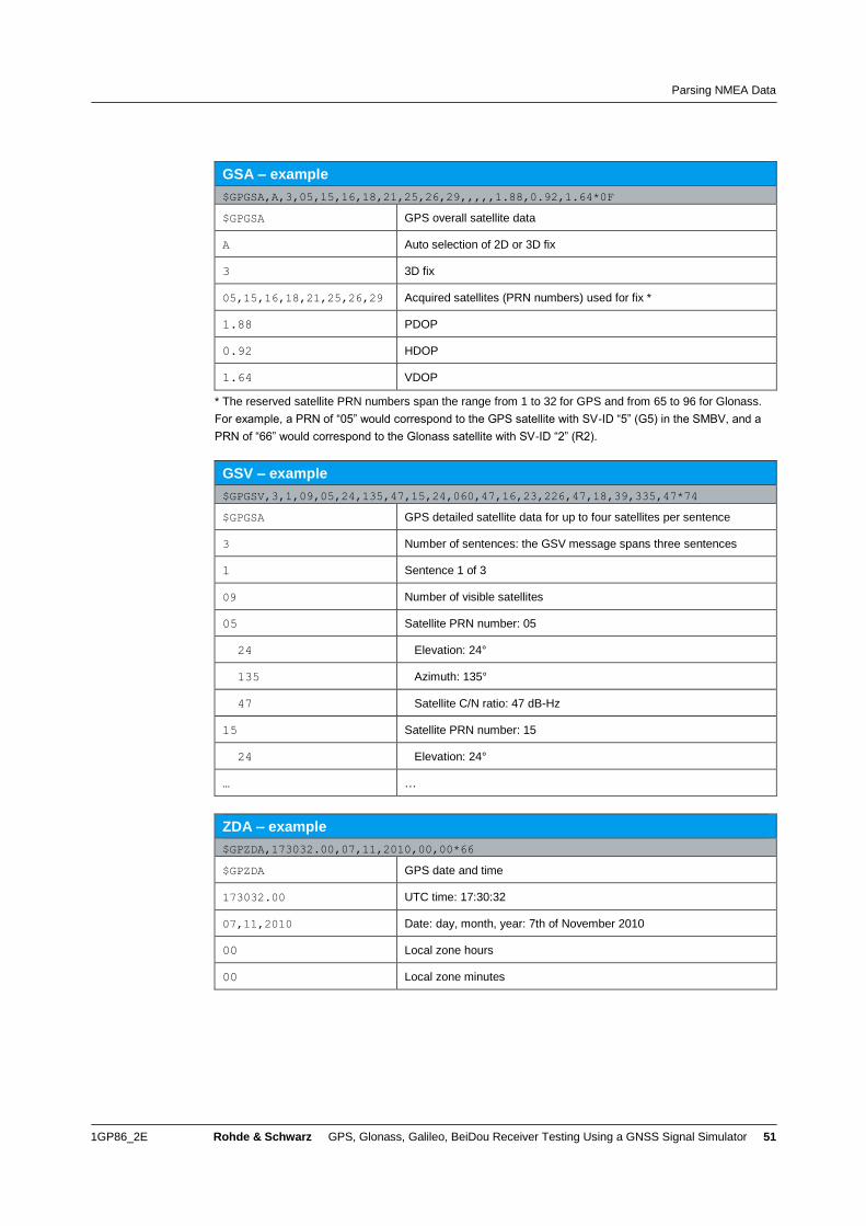
Parsing NMEA Data
1GP86_2E Rohde & Schwarz GPS, Glonass, Galileo, BeiDou Receiver Testing Using a GNSS Signal Simulator 51
GSA – example
$GPGSA,A,3,05,15,16,18,21,25,26,29,,,,,1.88,0.92,1.64*0F
$GPGSA GPS overall satellite data
A Auto selection of 2D or 3D fix
3 3D fix
05,15,16,18,21,25,26,29 Acquired satellites (PRN numbers) used for fix *
1.88 PDOP
0.92 HDOP
1.64 VDOP
* The reserved satellite PRN numbers span the range from 1 to 32 for GPS and from 65 to 96 for Glonass.
For example, a PRN of “05” would correspond to the GPS satellite with SV-ID “5” (G5) in the SMBV, and a
PRN of “66” would correspond to the Glonass satellite with SV-ID “2” (R2).
GSV – example
$GPGSV,3,1,09,05,24,135,47,15,24,060,47,16,23,226,47,18,39,335,47*74
$GPGSA GPS detailed satellite data for up to four satellites per sentence
3 Number of sentences: the GSV message spans three sentences
1 Sentence 1 of 3
09 Number of visible satellites
05 Satellite PRN number: 05
24 Elevation: 24°
135 Azimuth: 135°
47 Satellite C/N ratio: 47 dB-Hz
15 Satellite PRN number: 15
24 Elevation: 24°
… …
ZDA – example
$GPZDA,173032.00,07,11,2010,00,00*66
$GPZDA GPS date and time
173032.00 UTC time: 17:30:32
07,11,2010 Date: day, month, year: 7th of November 2010
00 Local zone hours
00 Local zone minutes
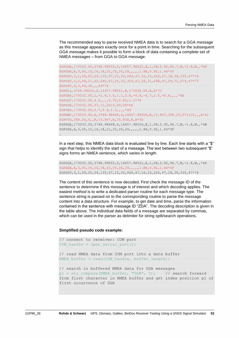
Parsing NMEA Data
1GP86_2E Rohde & Schwarz GPS, Glonass, Galileo, BeiDou Receiver Testing Using a GNSS Signal Simulator 52
The recommended way to parse received NMEA data is to search for a GGA message
as this message appears exactly once for a point in time. Searching for the subsequent
GGA message makes it possible to form a block of data containing a complete set of
NMEA messages – from GGA to GGA message.
$GPGGA,173032.00,3748.99055,S,14457.98521,E,1,08,0.92,96.7,M,-1.8,M,,*66
$GPGSA,A,3,05,15,16,18,21,25,26,29,,,,,1.88,0.92,1.64*0F
$GPGSV,3,1,09,05,24,135,47,15,24,060,47,16,23,226,47,18,39,335,47*74
$GPGSV,3,2,09,21,62,240,47,25,22,353,47,26,21,098,47,29,71,079,47*77
$GPGSV,3,3,09,30,,,43*74
$GPGLL,3748.99055,S,14457.98521,E,173032.00,A,A*7C
$GPGRS,173032.00,1,-1.9,1.0,1.1,2.6,-0.8,-4.7,2.0,-0.4,,,,*4A
$GPGST,173032.00,4.5,,,,0.70,0.85,1.3*74
$GPZDA,173032.00,07,11,2010,00,00*66
$GPGBS,173032.00,0.7,0.9,1.3,,,,*49
$GPRMC,173033.00,A,3748.98668,S,14457.98506,E,13.947,358.25,071110,,,A*41
$GPVTG,358.25,T,,M,13.947,N,25.830,K,A*30
$GPGGA,173033.00,3748.98668,S,14457.98506,E,1,08,0.92,96.7,M,-1.8,M,,*6B
$GPGSA,A,3,05,15,16,18,21,25,26,29,,,,,1.88,0.92,1.64*0F
…
In a next step, this NMEA data block is evaluated line by line. Each line starts with a “$”
sign that helps to identify the start of a message. The text between two subsequent “$”
signs forms an NMEA sentence, which varies in length.
$GPGGA,173032.00,3748.99055,S,14457.98521,E,1,08,0.92,96.7,M,-1.8,M,,*66
$GPGSA,A,3,05,15,16,18,21,25,26,29,,,,,1.88,0.92,1.64*0F
$GPGSV,3,1,09,05,24,135,47,15,24,060,47,16,23,226,47,18,39,335,47*74
The content of this sentence is now decoded. First check the message ID of the
sentence to determine if this message is of interest and which decoding applies. The
easiest method is to write a dedicated parser routine for each message type. The
sentence string is passed on to the corresponding routine to parse the message
content into a data structure. For example, to get date and time, parse the information
contained in the sentence with message ID “ZDA”. The decoding description is given in
the table above. The individual data fields of a message are separated by commas,
which can be used in the parser as delimiter for string split/search operations.
Simplified pseudo code example:
// connect to receiver: COM port
COM_handle = open_serial_port();
// read NMEA data from COM port into a data buffer
NMEA_buffer = read(COM_handle, buffer_length);
// search in buffered NMEA data for GGA messages
p1 = str_compare(NMEA_buffer, "GGA", 0); // search forward
from first character in NMEA buffer and get index position p1 of
first occurrence of GGA
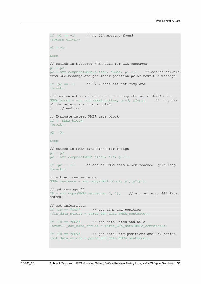
Parsing NMEA Data
1GP86_2E Rohde & Schwarz GPS, Glonass, Galileo, BeiDou Receiver Testing Using a GNSS Signal Simulator 53
If (p1 == -1) // no GGA message found
{return error;}
p2 = p1;
Loop
{
// search in buffered NMEA data for GGA messages
p1 = p2;
p2 = str_compare(NMEA_buffer, "GGA", p1+1); // search forward
from GGA message and get index position p2 of next GGA message
If (p2 == -1) // NMEA data set not complete
{break;}
// form data block that contains a complete set of NMEA data
NMEA_block = str_copy(NMEA_buffer, p1-3, p2-p1); // copy p2-
p1 characters starting at p1-3
} // end loop
// Evaluate latest NMEA data block
If (! NMEA_block)
{break;}
p2 = 0;
Loop
{
// search in NMEA data block for $ sign
p1 = p2;
p2 = str_compare(NMEA_block, "$", p1+1);
If (p2 == -1) // end of NMEA data block reached, quit loop
{break;}
// extract one sentence
NMEA_sentence = str_copy(NMEA_block, p1, p2-p1);
// get message ID
ID = str_copy(NMEA_sentence, 3, 3); // extract e.g. GGA from
$GPGGA
// get information
If (ID == "GGA") // get time and position
{fix_data_struct = parse_GGA_data(NMEA_sentence);}
If (ID == "GSA") // get satellites and DOPs
{overall_sat_data_struct = parse_GSA_data(NMEA_sentence);}
If (ID == "GSV") // get satellite positions and C/N ratios
{sat_data_struct = parse_GSV_data(NMEA_sentence);}
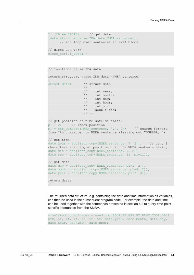
Parsing NMEA Data
1GP86_2E Rohde & Schwarz GPS, Glonass, Galileo, BeiDou Receiver Testing Using a GNSS Signal Simulator 54
If (ID == "ZDA") // get date
{date_struct = parse_ZDA_data(NMEA_sentence);}
} // end loop over sentences in NMEA block
// close COM port
close_serial_port();
// function: parse_ZDA_data
return_structure parse_ZDA_data (NMEA_sentence)
{
struct date; // struct date
// {
// int year;
// int month;
// int day;
// int hour;
// int min;
// double sec;
// };
// get position of time-date delimiter
p1 = 0; // index position
p1 = str_compare(NMEA_sentence, ",", 7); // search forward
from 7th character in NMEA sentence (leaving out "$GPZDA, ")
// get time
date.hour = atoi(str_copy(NMEA_sentence, 7, 2)); // copy 2
characters starting at position 7 in the NMEA sentence string
date.min = atoi(str_copy(NMEA_sentence, 9, 2));
date.sec = atof(str_copy(NMEA_sentence, 11, p1-11));
// get date
date.day = atoi(str_copy(NMEA_sentence, p1+1, 2));
date.month = atoi(str_copy(NMEA_sentence, p1+4, 2));
date.year = atoi(str_copy(NMEA_sentence, p1+7, 4));
return date;
}
The returned data structure, e.g. containing the date and time information as variables,
can then be used in the subsequent program code. For example, the date and time
can be used together with the commands presented in section 6.2 to query time-point-
specific information from the SMBV.
simulated_coordinates = send_cmd(SOUR:BB:GPS:RT:RLOC:COOR:DEC?
UTC, %f, %f, %f, %f, %f, %f; date.year, date.month, date.day,
date.hour, date.min, date.sec);
Summary
1GP86_2E Rohde & Schwarz GPS, Glonass, Galileo, BeiDou Receiver Testing Using a GNSS Signal Simulator 55
8 Summary GNSS receivers can be tested easily, reliably and cost-efficiently by using the SMBV
as satellite simulator. GPS, Glonass, Galileo, and BeiDou signals for up to 24 satellites
can be generated in realtime with a single standalone instrument. This sets new
standards in the field of satellite simulation for R&D and production.
In this application note, we explained how to perform automated receiver tests. Various
fundamental tests including TTFF, sensitivity and location accuracy as well as moving
receiver, interference and multipath tests are described. For each test, we provided a
basic remote control example to show how to correctly configure the SMBV.

Abbreviations
1GP86_2E Rohde & Schwarz GPS, Glonass, Galileo, BeiDou Receiver Testing Using a GNSS Signal Simulator 56
9 Abbreviations 2D Two-dimensional
3D Three-dimensional
A-GPS Assisted GPS
AWGN Additive white Gaussian noise
BeiDou BeiDou (Chinese satellite navigation system)
CW Continuous wave
C/A code Coarse acquisition code
C/N Carrier to noise
DC Direct current
DOP Dilution of precision
GDOP Geometric DOP
HDOP Horizontal DOP
PDOP Positional DOP
TDOP Time DOP
VDOP Vertical DOP
DUT Device under test
ECEF Earth centered, earth fixed
ENU East north up
Galileo Galileo (global navigation satellite system of the European
Union)
Glonass Globalnaja Nawigazionnaja Sputnikowaja Sistema (global
navigation satellite system of the Russian Federation)
GNSS Global navigation satellite system (stands for all satellite-
based navigation systems)
GPIB General purpose interface bus
GPS Global positioning system (of the United States of America)
GPS CA Global positioning system coarse acquisition code
GUI Graphical user interface
HIL Hardware in the loop
ID Identifier
KML Keyhole markup language
LAN Local area network
LNA Low noise amplifier
LOS Line of sight
NED North east down
NMEA National Marine Electronics Association
P code Precision code
R&D Research and development
RF Radio frequency
RAIM Receiver autonomous integrity monitoring
RINEX Receiver independent exchange format
USB Universal serial bus
UTC Universal time coordinated
SCPI Standard commands for programmable instruments
SPOT Satellites and position online tracker (in the SMBV)
SV-ID Space vehicle ID
TTL Transistor–transistor logic
VNC Virtual network computing
XML Extensible markup language
References
1GP86_2E Rohde & Schwarz GPS, Glonass, Galileo, BeiDou Receiver Testing Using a GNSS Signal Simulator 57
10 References [1] Rohde & Schwarz, “Satellite Navigation Digital Standard for R&S
®SMBV and
R&S®WinIQSIM2
TM” Operating Manual
[2] Rohde & Schwarz Application Note, “Time Synchronous Signals with Multiple
R&S®SMBV100A Vector Signal Generators” (1GP84)
[3] Rohde & Schwarz Application Note, “R&S ARB Toolbox Plus” (1GP88)
[4] Rohde & Schwarz Application Note, “R&S dB Calculator” (1GP77)
[5] Rohde & Schwarz Application Note, “Top Ten SCPI Programming Tips for
Signal Generators” (1GP79)
[6] Rohde & Schwarz Application Note, “Connectivity of Rohde & Schwarz Signal
Generators” (1GP72)
[7] Rohde & Schwarz Application Note, “Simulating Automatic Obscuration and
Multipath for Realistic GNSS Receiver Testing” (1GP101)
[8] Rohde & Schwarz Application Note, “Hardware in the Loop (HIL) Tests with a
GNSS Simulator” (1GP102)
Up-to-date almanac data can be downloaded for example at:
www.navcen.uscg.gov
www.celestrak.com/GPS/almanac/
11 Ordering Information Please visit the R&S
®SMBV100A product website for comprehensive ordering
information at www.rohde-schwarz.com.

About Rohde & Schwarz
Rohde & Schwarz is an independent group
of companies specializing in electronics. It is
a leading supplier of solutions in the fields of
test and measurement, broadcasting,
radiomonitoring and radiolocation, as well as
secure communications. Established more
than 75 years ago, Rohde & Schwarz has a
global presence and a dedicated service
network in over 70 countries. Company
headquarters are in Munich, Germany.
Environmental commitment
● Energy-efficient products
● Continuous improvement in
environmental sustainability
● ISO 14001-certified environmental
management system
Regional contact
Europe, Africa, Middle East
+49 89 4129 123 45
[email protected] North America
1-888-TEST-RSA (1-888-837-8772)
[email protected] Latin America
+1-410-910-7988
[email protected] Asia/Pacific
+65 65 13 04 88
[email protected] China
+86-800-810-8228 /+86-400-650-5896
This application note and the supplied
programs may only be used subject to the
conditions of use set forth in the download
area of the Rohde & Schwarz website.
R&S® is a registered trademark of Rohde & Schwarz GmbH & Co. KG. Trade names are trademarks of the owners.
Rohde & Schwarz GmbH & Co. KG
Mühldorfstraße 15 | D - 81671 München
Phone + 49 89 4129 - 0 | Fax + 49 89 4129 – 13777
www.rohde-schwarz.com