RE

PO

RT

82011

GPR-measurements of snow distribution on Hardangervidda mountain plateau in 2008-2011Galina Ragulina, Kjetil Melvold, Tuomo Saloranta

GPR-measurements of snow distribution on Hardangervidda mountain plateau in 2008-2011

Norwegian Water Resources and Energy Directorate 2012

Report no. 8 – 2011

GPR-measurements of snow distribution on Hardangervidda mountain plateau in 2008-2011

Published by: Norwegian Water Resources and Energy Directorate

Authors: Galina Ragulina, Kjetil Melvold, Tuomo Saloranta

Print: Norwegian Water Resources and Energy Directorate Number

printed: 36

Cover photo: Kjetil Melvold

ISSN: 1502-3540

ISBN: 978-82-410-0773-6 Abstract: Results of snow depth GPR-measurements performed at

Hardangervidda mountain plateau in 2008-2011 are presented in this report. The paper consists of both fieldwork description and data analyses. Our statistical manipulations with the data are also described.

Key words: Snow, Snow depth, Ground Penetrating Radar, GPR, Snow distribution, Meteorology

Norwegian Water Resources and Energy Directorate

Middelthunsgate 29 P.O. Box 5091 Majorstua N 0301 OSLO

NORWAY Telephone: +47 22 95 95 95

Fax: +47 22 95 90 00 E-mail: nve@nve.no Internet: www.nve.no

November 2011

Contents Preface ................................................................................................. 4 

Summary ............................................................................................. 5 

1  Introduction ................................................................................... 6 

2  Instruments and methods (fieldwork data processing) ............ 9 

2.1  GPR principle of operating ............................................................... 9 2.2  GPR-parameter settings ................................................................ 10 2.3  Field setup ...................................................................................... 11 

3  Data analysis/processing ........................................................... 13 

3.1  Data logging ................................................................................... 13 3.2  Navigation ...................................................................................... 13 3.3  Digitalisation of raw radargrams ..................................................... 13 3.4  Coupling GPR and GPS ................................................................. 15 3.5  From TWT to snow depth ............................................................... 16 3.6  Limitations due to coupling pulse and its effects ............................ 17 

4  Results and discussion .............................................................. 21 

4.1  The overall snow conditions ........................................................... 21 4.2  Distribution fitting and imputation of values below detection limit in snow depth observations ......................................................................... 26 

Conclusions ...................................................................................... 31 

References......................................................................................... 32 

4

Preface As a part of the internal FOU project BREMS (Bedre Romlige Estimater av

Meteo-hydrologiske Synoptiske felt) two 80 km long snow courses were established on Hardangervidda in southern Norway in 2008. One of the snow courses was also measured in 2010 and 2011. Both laser scanning and Ground Penetrating Radar (GPR) were selected as tools to determine snow depth along the snow courses.

The purpose of this report is to provide a joint presentation of the GPR investigations carried out in 2008, 2010 and 2011. It gives a short introduction to the method and describes data collecting and post-processing steps for the GPR in order to derive snow depth. Due to limitation with the GPR-system shallow snow cover (less then 35 cm) is absent in the digitalised dataset. In order to replace these missing values with some plausible estimates, we used statistical imputation methods.

The overall snow condition along the transect system has been described and further compared with SeNorge model estimates.

The authors thank warmly all the people and organisations (“Hardangervidda Villreinutval”, “Hardangervidda fjelloppsyn AS”) who have been involved in fieldwork in 2008, 2009, 2010 and 2011. We will also thank the Hordaland and Buskerud “Tilsynsutvalg” for permission to carry out the fieldwork in Hardangervidda National Park.

Oslo, November 2011 Morten Johnsrud Director, Hydrology Department

Rune Engeset Head of Section, Section for Glaciers, Snow and Ice

5

Summary Hardangervidda, situated in southern Norway, is one of Europe’s largest mountain

plateaus. Most of the plateau is over 1000 m above sea level, and snow conditions on Hardangervidda are important for aspects such as hydropower production and recreation, and for the population dynamics of wild reindeer and trout. To investigate snow conditions on Hardangervidda, the Norwegian Water Resources and Energy Directorate (NVE) has conducted yearly snow measurement campaigns across Hardangervidda since 2008 using Ground Penetrating Radar (GPR) at the approximate time of annual snow maximum (mid-April). These measurements also provide valuable data for calibration of snow models, such as the seNorge model (www.senorge.no). We present snow distribution along west-east transects across Hardangervidda for three years (2008, 2010 and 2011).

Collected data in the form of radargrams were first digitalised and the digital data were averaged to 2, 10, 20 and 100-metre mean values. Measurements over hydrological features (such as small lakes) were filtered away. An empirical method was used for the calculation of snow depth.

The snow distribution over Hardangervidda was analysed both by longitudinal profiles and by separating western and eastern parts. We found a significant west-east trend in snow distribution and almost no difference in the north-south direction. It was also shown that the SeNorge model significantly overestimates snow depth values compared to the GPR-measurements.

Investigation of data revealed a limitation in the GPR-measurements, as snow depths less than 25-35 cm for 350 MHz-antenna and 15-25 cm for 1000 MHz-antenna were not readily possible to interpret. To rectify this problem, a statistical imputation method was used to replace missing values below this detection limit, and new statistics were calculated. Future fieldwork procedure should also be modified in order to better sample areas of low snow depth and bare ground.

Most of the constructed snow depth distributions have a two-peak shape. However it remains unclear whether the secondary peak is a real feature, i.e. a significant low snow depth population or large bare ground fraction, or merely an artefact of the GPR data. A closer investigation of this issue could improve our knowledge of the nature of snow depth distribution in mountain plateaus, and on the sampling and interpretation of GPR-based snow measurements.

6

1 Introduction

This report consists of the description and analysis of snow data collected on Hardangervidda, Norway, in spring 2008, 2010 and 2011.

Hardangervidda, situated in the Western part of Southern Norway (Figure 1), is one of Europe’s largest mountain plateaus. Most of the plateau is over 1000 m above sea level, and snow conditions on Hardangervidda are important for aspects such as hydropower production and recreation. Snow cover and thickness pattern also influence the reindeer semi-nomadic use of the living areas. Studies by Stand et al. (2006) indicate that snow depth is an important factor in explaining the reindeer winter habitat use pattern. Snow cover and snow depth affect growing season and plant distributions (Odland and Munkejord, 2008) and on lakes the spring snow depth effects the growth of brown trout (Borgstrøm, 2001).

Figure 1 – Position of Hardangervidda National park and measurement profiles in 2008.

Hardangervidda covers an area of about 6500 km2; almost 3500 km2 of this is situated in the Hardangervidda National Park. In the area there were no records of meteorological measurements before a project started in 2008 and few snow measurements available.

The evaluation of the SeNorge.no snow model against snow course, snow pillows and catchment model simulation data by Engeset et al. (2004) indicate an

7

overestimation of SWE in the areas close to Hardangervidda, where the SeNorge model shows a strong east-west gradient in snow depth. The lack of data for calibration of the SeNorge model from this area became the main reason to run the measurement project on Hardangervidda. Another reason was a low level of anthropogenic influence over the territory because of the National Park (NP) restrictions.

The original plan for the project called BREMS1 was to use airborne (by helicopter) Ground Penetrating Radar (GPR) survey to measure snow depth over the area. However, permission to carry out helicopter flights over Hardangervidda NP was not given by the National park administration, and because of that the plan was changed. Measurements with GPR from helicopter were exchanged with an airborne laser scanning2 (airborne laser scanning gives only snow depth). Since ground-based snow density measurements were needed in order to convert snow depth to water equivalent a field program was necessary. Since all the necessary equipment was available at the moment, it was decided to carry out ground-based GPR survey in connection with a snow density measurement program. Thereby two different methods were used to measure the snow depth simultaneously in order to be able to compare the results from both ones afterwards. This report consists of the GPR-method only.

The BREMS project was planned with two field seasons 2008 and 2009. However, it initiated a series of annual GPR-measurements on Hardangervidda. In addition, snow density samples (SDS) were taken approximately every second kilometre along the GPR-profile at the same field work period. Field work took place in the end of the snow accumulation period (close to snow maximum), just before the melting usually starts in the area (mid-April), and lasted usually 2 days.

List of participants, field work periods, GPR-measured distance and amount of SDS-points are presented in Table 1.

1 Bedre Romlige Estimater av Meteo-hydrologiske Synoptiske felt (Better Spatial Estimates of Meteo-hydrological Synoptic field) 2 All the details of the laser scanning investigation can be found in K. Melvold. Unpublished.

8

Date Participants GPR-

measured distance

Amount of SDS-points

2008,

15-16 of

April

Kjetil Melvold (NVE), Stein H. Flaata,

Heidi Bache Stranden (NVE), Anve K. Myklatun,

Ånund Kvambekk (NVE), Ragnar Ystanes,

Zelalem Mengustu (NVE), Jon Mårdalen

136 km

70

2009,

16-17 of

April

Kjetil Melvold (NVE), Anders Vaksdal,

Frode Randen (NVE), Anve K. Myklatun,

Heidi Bache Stranden (NVE), Georg Gjørstein

-

(difficult snow

conditions)

28

2010,

13-14 of

April

Kjetil Melvold (NVE), Sveinung H. Olsnes,

Ånund Kvambekk (NVE), Georg Gjørstein

90,1 km

39

2011,

13-14 of

April

Kjetil Melvold (NVE), Heidi Bache Stranden (NVE),

Tuomo Saloranta (NVE), Galina Ragulina (NVE)

71,7 km

25

Table 1 – Some field work information.

9

2 Instruments and methods (fieldwork data processing)

2.1 GPR principle of operating

The GPR (impulse radar system) can be used as a tool in snowpack studies for measuring e.g. snow depth and snow layering structure. The basic principle of this active geophysical method is to transmit electromagnetic pulses of suitable frequency down into the ground through a transmitting antenna, and to detect the reflected energy as a function of time, amplitude and phase from any subsurface targets through a receiver antenna. If the electromagnetic travel velocity of the subsurface is known, time can be converted to a depth.

As the electromagnetic waves propagate into the ground, the power decreases as the inverse square of distance. Wave reflections are generated from the boundaries of materials of different electromagnetic properties. The large contrast between the electromagnetic properties of rock, ice, water, and some sediment makes GPR a particularly effective method for mapping snow structure. However, reflections may also originate from anisotropy due to fine layering or density variations of a single material, or from objects on the surface creating an interference pattern.

SIR-3000 GPR system from GSSI3 was used for this study together with 350 and 1000 MHz antennae.

GPR utilizes an antenna (consisting of a transmitter and receiver a small fixed distance apart) to send electromagnetic waves into the subsurface (Figure 2). The antenna is moved over the surface of the snow to be inspected. The transmitter sends a diverging beam of energy pulses into the subsurface and the receiver collects the energy reflected from interfaces between media of differing electrical properties. The reflected energy is recorded as a function of time, and the time delay (between transmitted and received signal) can be converted to a depth by multiplying with speed of the electromagnetic waves through the media. The radargrams constitute the raw GPR-data. They are displayed in real time on the control unit (Figure 2). Basic interpretation can be conducted on site (http://www.sandberg.co.uk/ground-radar/gpr-principles.html). In our case however, the radargrams were processed and analyzed off-site using specialist software – ReflexW 5.5.

There are two basic considerations that must be made when planning a GPR survey: the desired depth penetration and the resolution needed for the problem at hand. The depth penetration of a radar system is not straightforward to predict. A basic

3 Geophysical Survey Systems, Inc.

10

requirement is that the reflected power received from an object must be strong enough to be detectable by the system. This can be evaluated by the radar range equation, which relates the received power from a scattering object to the transmitting power, antenna gain and the distance to the object, and by the signal to noise ratio of the receiver. However, many of the parameters in the radar equation are generally not known. GPR system characteristics, such as performance factor and antenna pattern provide basic constraints, while the electrical properties of the ground, character and size of the reflector in question are site-dependent constraints. With respect to resolution, both the horizontal and the vertical resolution must be considered. The basic decision to be made is that of antenna centre frequency. In general, low frequency systems are more penetrating, but data resolution is lower; high frequency systems have limited penetration but offer a higher resolution. The choice of antenna frequencies is therefore very much dependent on snowpack conditions (both snow depth and liquid water content). For the snowpack which is deeper than 2 m, frequency systems from 1 GHz and lower are normally used.

2.2 GPR-parameter settings

Depending on the specific GPR system used, a number of parameters may be determined by the user to optimize data collection. The time window (RANGE in SIR-3000) determines how long the system will record signals from the receiver antenna after a pulse has left the transmitter antenna (length of trace). The necessary time window can be found by considering the maximum depth and the minimum velocity likely to be encountered. Each trace is made up of a set number of individual data points, called Samples. The Sample interval determines how often the signal that is received is measured, and thus how well its form is represented. The frequency must be at least twice as high as the highest frequency of the signal, in order to reproduce this correctly. With a factor of safety of two, the sampling frequency should be at least 6 times the centre frequency of the antennae, to be able to get real vertical resolution. As sample rate increases, the scan rate drops and file size increases.

With horizontal stacking, the GPR systems perform a user-determined number of measurements of a target and then average these traces. Stacking will in general improve the signal to noise ratio, but a large number of stacks may also introduce noise if the GPR system is moved too far from the target since the target will not be in focus anymore.

SeNorge simulations indicated that the western part of Hardangervidda usually was covered with deeper snow than the eastern part. The use of 1000 MHz antenna with a large time window of 100 ns (approximate 10 m of snow) and one scan per 10 cm was rather unpractical in the western part, due to system limitation (in case of not very slow driving, the system becomes “overloaded” and drops individual scans). In addition,

11

rather high liquid water content in the snow leads to reduced penetration depth of the radar signal. This effect is more pronounced for the 1000 MHz antenna than for the 350 MHz one. Those and a large snow-GPR operating personal experience of the project leader Kjetil Melvold were the reasons to chose a 350 MHz antenna for the deep or wet snow.

In order to prevent spatial aliasing (missing important horizontal structures due to low sampling density) the GPR was set to sample every 20 cm whenever the 350 MHz antenna was used, and every 10 cm whenever using the 1000 MHz antenna. The sampling was controlled by the use of the distance wheel. During the establishment of the snow survey in 2008 a 10 cm sampling interval was used for both 350 and 1000 MHz antennas.

Figure 3 – Radar-train.

2.3 Field setup

The measuring procedure includes the so-called “Radar-train” (Figure 3), consisting of a snow mobile in front with a driver and a radar operator (passenger), a GPS4-antenna, a covered radar-sledge (GPR-antenna + GPR-battery) and a distance wheel at the back. This radar-train attempts to follow a fixed route with the help of GPS navigation. Navigation was carried out by handheld Garmin GPS.

4 Global Positioning System

A driver and navigator

A passenger and Radar-operator

GPS-antenna Figure 2 – Ground Penetrating Radar.

12

The driver is responsible for smooth driving along the fixed route, while the radar operator is operating the radar software and watching that GPR-data are sampled without errors and gaps. The GSSI SIR 3000 system enables the user to tick-mark locations or special features during continuous profiling. It was found useful to use this option for example when the radar crosses over snow-free areas. Making marks and remembering their meaning while driving from one GPS-waypoint to the next is not an easy task, but necessary (for a detailed explanation of the phenomenon, see Chapter 3.6 “Limitations due coupling pulse and it effects”). The meaning of every mark made is written down in the field work notebook at the first stop, and a manual snow depth sounding is performed. These manual soundings were performed just by the side of the GPR-antenna at every stop in 2010 and 2011, while in 2008 no such measurement were carried out. These manual snow depth soundings are used for both calibrating and as an aid while digitalizing raw radargrams.

Fixed waypoints are situated approximately every 2 km along two 80 km latitudinal profiles (Figure 4). A new data file is started at every waypoint, so that the files do not become too large and heavy for further processing. Nevertheless, it may be necessary to stop between waypoints to take extra manual snow depth soundings (a new file is usually not created then).

Profile 1 was GPR-measured only once in 2008 and only last 50 km, due to a very rough terrain in the western part of this profile.

Figure 4 – Positioning of Waypoints by Profiles.

Profile 1

Profile 2

13

3 Data analysis/processing

3.1 Data logging

Data collected during the field work, such as manual measurements of snow depth and bulk density, radar description and all corresponding information and comments during survey were written down in the so-called “description files” (Excel-files).

Differential GPS (DGPS) post-processing (see Chapter 3.2 for details) was carried out by Bjarne Kjøllmoen (Senior Engineer at the Glacier, Ice and Snow Section, Hydrology Department, Norwegian Water Resources and Energy Directorate (NVE), Norway) for every measured year. The Norwegian Mapping Authority base station Dagali was used as a reference GPS in 2008 – 2010 and Maurset in 2011.

3.2 Navigation

Navigation was carried out by handheld Garmin GPS. For the accurate positioning and timing of the survey path one GP-3 TOPCON GPS receiver was used in addition to GPS data from a known reference station. The GPS measurements were stored in the GPS receivers, and were subsequently transferred to a computer running the GPS post-processing software. The software computed baselines using simultaneous measurement data from both GPS receivers (used during survey and the fixed one5) and came out with precise positioning of measurement track. Positioning was calculated using the DGPS post-processing method. DGPS is an enhancement to GPS that provides improved location accuracy, from the 15-meter nominal GPS accuracy to about 10 cm in case of the best implementations. DGPS uses a network of fixed, ground-based reference stations to broadcast the difference between the positions indicated by the satellite systems and the known fixed positions. Post-processing is used in DGPS to obtain precise positions of unknown points by relating them to fixed, ground-based reference stations such as survey markers. Such a method allows more precise positioning, because most GPS errors affect each receiver nearly equally and therefore can be cancelled out in the calculations.

3.3 Digitalisation of raw radargrams

66 data-files with raw radargrams were collected in 2008, 40 files in 2010 and 26 files in 2011. As it was already mentioned in Chapter 2, every file in general consists of 2 – 3 km long transects of GPR-measurements.

It was Dagali in 2008 – 2010 and Maurset in 2011

14

Original *.dzt raw data-files (GSSI radar format) were imported into Reflex-software. ReflexW PreVersion 5.5 from 01.01.2010 (copyright by K. J. Sandmeier) was used for processing and interpretation of radar data and for digitalising radargrams.

At a preliminary stage of digitalisation, filtering options such as substruct-mean (dewow), static correction and manual gain (for few files), were applied.

Digitalisation of processed radargrams is a difficult and time-consuming process. The task is to recognize the “correct” reflector among all “noise”-reflectors. It is possible to use so called automatic phase-follower. However GPR was not driven over an even surface but over a rough terrain. This created many small hyperbolae which resulted in a “jumping”-reflector with many ups and downs. Migration was tested for removing some of the hyperbolae in the radar reflector without significant improvement. The hyperbolae make it very difficult for the automatic phase-follower: whenever such a “jump” appears in a radargram, the follower also jumps and continues on a wrong track. This means that it is impossible to trust the automatic follower completely and most of the work must be done manually. The example in Figure 5 illustrates some of these difficulties.

Figure 5 – An example of a radargram from 1000 MHz-antenna set (2008, Profile 1. Upper

radargram is already digitalised; lower one is the same radargram before

digitalisation. Green ovals point up the areas with “jumping”-reflector.

Both Figures 5 and 6 show that it is not only an interrupted reflector line that makes it difficult for digitalising, but also a necessity of making a choice for the “correct” reflector (green circles). Both knowledge and experience are often needed to make such a decision.

15

Figure 6 – An example of a radargram from 350 MHz-antenna set (2008, Profile 2). The

upper radargram is digitalised; the lower one is the same radargram before

digitalisation. Purple circles illustrate areas with a detection limit problem.

Green circles point out the areas with several strong reflectors at the same time.

Additional challenge is connected with data resolution given by the used antennas. If higher frequency 1000 GHz antenna allows to see snow depth which is deeper than app. 14-23 cm, lower frequency 350 MHz-antenna system can only show snow depth which is deeper than 25-35 cm (depending on the snow condition). To be able to analyse snow distribution on Hardangervidda in 2008 – 2011 without losing an important part of the data, snow depths below DL were not digitalised but set to “zero” depth (purple circles on Figure 6). Detailed explanation of the phenomenon can be found in Chapter 3.6 “Limitations due to coupling pulse and its effects”.

3.4 Coupling GPR and GPS

Excel Macros (programmed in Visual Basic by Kjetil Melvold) were used to convert the digitalised GPR data from .PCK-format (given by ReflexW-software) to the wider used .XLS-format. After this conversion, the digitalised GPR-data were coupled with GPS-data for correct positioning.

Every file (2.5 – 3 km with GPR-measurements) consists of 15-30 thousand lines with information (XY-coordinates, TWT6, distance from the beginning of the file etc). Considering the fact that one measured profile (Figure 7) consists of 30-40 such files, it is understandable that some averaging was needed to work further with the dataset. Therefore 2, 10, 20 and 100-m mean values were calculated. Finally, the individual files were merged together by measurement Profiles 1 and 2 from west to east.

6 Two – Way – Travel time. The time taken for a radio signal to travel from the transmitter down to a reflector (subsurface) and back to a receiver at the surface.

16

3.5 From TWT to snow depth

Based on the TWT the snow depth (SD) was calculated by:

, where represents a phase velocity of the radar wave.

For dry snow it is possible to estimate by using an empirical formula of the relative real dielectric constant for snow, which is dependent on the specific density (no unit) of snow (Kovacs et al., 1995). This method requires a good estimate of the snow density over the measurement area.

This study uses a different empirical method. In order to estimate , independently measured snow depths at the same locations as GPR-measurements were

plotted against the corresponding values of and a linear regression line was fitted to

the data (Figure 7). Snow properties in 2008 were different with dryer snow than in 2010-2011. In 2008 no manual sounding was carried out next to the GPR-antenna, however there is indirect information about the snow depth from laser scanning data. That is why the estimation of was done separately for 2008 and 2010-2011.

The difference between velocities in 2008 and 2010-2011 appeared to be rather small (Figure 7). Because of that it was decided to use the same velocity 215 mm/ns for all the years with measurements.

Figure 7 – Linear regression lines for the relations between independently measured snow depth (SD) and TWT in 2008 and 2010-2011.

y = 215,16xR² = 0,9363

0

1000

2000

3000

4000

5000

6000

0,00 10,00 20,00 30,00

Laser‐measured SD, m

m

TWT (Two‐Way‐Travel time)/2,mm/ns

2008

SD vs TWT/2

Lineær (SD vs TWT/2)

y = 214,75xR² = 0,9645

0

500

1000

1500

2000

2500

3000

3500

4000

0,00 10,00 20,00

SD from snow sounding, m

m

TWT (Two‐Way‐Travel time)/2,mm/ns

2010 ‐ 2011

SD vs TWT/2

Lineær (SD vs TWT/2)

17

At the time of surveys all lakes and rivers were frozen and snow covered. GPR-measuring was performed with no regard to those hydrological objects. A large amount of the GPR survey was therefore carried out on top of lakes or rivers since there are many such water bodies on Hardangervidda. There is a significant difference in the backscattering of the radar signal from data collected on the top of the snow cover over water bodies compared with data collected over dry land. It occurs because the presence of water has a substantial influence on the radio signal penetrating and reflecting strength, which can not be neglected. Description of the phenomenon can be found in Hamran (1996).

Based on the GPR-field survey it is not possible to determine the snow depth that is carried out over water bodies. In order to exclude a possible influence of water presence on the collected data, “hydrological object filtration” was performed on both Profile 1 and 2 for every measurement year. In other words, data were uploaded to ArcMap GIS-software together with the precise information of hydrological objects position, and measurements intersecting those water bodies were deleted from the dataset.

3.6 Limitations due to coupling pulse and its effects

In a bistatic GPR system the transmitted and receiving antennas are placed next to each other (typical 50-100 mm apart). Because of this configuration, a portion of the transmitted electromagnetic energy is passed directly from a transmitter to a receiver without undergoing any reflections. In the time domain this energy will reflect to a pulse at the beginning of the scan. These pulses are commonly referred to in the literature as “direct wave” or “coupling pulse”. For a ground-based GPR system shallow reflectors entirely overlap the coupling pulse. In addition ringing in the antenna will also mask real reflectors. The ringing of GPR signal is caused by the resonance of the antenna. For the 350 MHz antenna snow depths less than 25-35 cm (depending on the snow conditions) are not readily possible to interpret. The strong direct signal just covers them on a radargram. In the more high frequency systems such as 1000 MHz-antenna, it is hard to detect snow depths less than 15-25 cm (depending on the snow conditions). In addition to the masking described above, it is not possible to determine from the radar signal if snow is present or not.

To rectify the latter problem it is essential to make notes whenever the radar passes over snow free areas. It is possible in the radar system to make tick-marks in the radar file to indicate areas without snow. Those tick-marks/stamps help to detect areas with no snow on the radargrams during digitalising. This procedure was applied for the measurement period in 2011.

It is also important to take the masking of shallow reflectors into account when digitising the data. In our first attempt to derived snow depth data from the GPR this

18

problem was not taken into account. Figure 8 shows frequency histograms of snow depth for all three years with measurements both separately and together. A close examination of Figure 8 shows a peak in snow depth frequency at about 35 cm for both 2008 and 2010 data. The peak is less pronounced in 2011 data. In order to investigate if this peak is a true feature of the snow distribution or an effect of the sampling method, the GPR data were redigitalised.

Figure 8 – Frequency histograms with 30 mm interval.

0,0

0,5

1,0

1,5

2,0

2,5

3,0

3,5

4,0

4,5

0900

1800

2700

3600

4500

5400

6300

7200

8100

9000

%

Snow depth, mm

2008

0

0,5

1

1,5

2

2,5

3

3,5

4

4,5

0900

1800

2700

3600

4500

5400

6300

7200

8100

9000

%

Snow depth, mm

2010

0,0

0,5

1,0

1,5

2,0

2,5

3,0

3,5

4,0

4,5

0900

1800

2700

3600

4500

5400

6300

7200

8100

9000

%

Snow depth, mm

2011

0,0

0,5

1,0

1,5

2,0

2,5

3,0

3,5

4,0

4,5

5,0

0300

600

900

1200

1500

1800

2100

2400

2700

3000

3300

3600

3900

4200

4500

4800

5100

5400

5700

6000

6300

6600

6900

7200

7500

7800

8100

8400

8700

9000

9300

9600

%

Snow depth, mm

2008

2010

2011

19

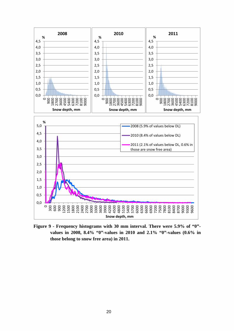
Since there were no tick-marks in 2008 and 2010, a new digitalisation of the “difficult areas” in the upper part of the radargrams (when the snow/ground reflector intersects the coupling pulse) was carried out. If snow depth was less than the detection limit, “0”-values were implemented. Those “0”-values give an estimate of how much of the snow depth was less than the minimum registered earlier. This minimum we call a detection limit (DL). Even though radargrams from 2011 had snow-free marks, snow depths between DL and areas with such marks are anyway not readily to interpret and were also digitalised as “0”.

Snow depth distribution after redigitalising can be seen in Figure 9. The first peak at about 35 cm has disappeared from both 2008 and 2010 histograms. All the histograms have rather rugged multi-peaked shape. In addition, there is a peak at about 75 cm in 2008 distribution. A plausible explanation for the multiple peaks could be thick ice layers in the snowpack that give strong reflectors in the GPR-signal, so that these reflectors could be mistakenly detected as the snow/ground interface.

20

Figure 9 - Frequency histograms with 30 mm interval. There were 5.9% of “0”-values in 2008, 8.4% “0”-values in 2010 and 2.1% “0”-values (0.6% in those belong to snow free area) in 2011.

0,0

0,5

1,0

1,5

2,0

2,5

3,0

3,5

4,0

4,50

900

1800

2700

3600

4500

5400

6300

7200

8100

9000

%

Snow depth, mm

2008

0,0

0,5

1,0

1,5

2,0

2,5

3,0

3,5

4,0

4,5

0900

1800

2700

3600

4500

5400

6300

7200

8100

9000

%

Snow depth, mm

2010

0,0

0,5

1,0

1,5

2,0

2,5

3,0

3,5

4,0

4,5

0900

1800

2700

3600

4500

5400

6300

7200

8100

9000

%

Snow depth, mm

2011

0,0

0,5

1,0

1,5

2,0

2,5

3,0

3,5

4,0

4,5

5,0

0300

600

900

1200

1500

1800

2100

2400

2700

3000

3300

3600

3900

4200

4500

4800

5100

5400

5700

6000

6300

6600

6900

7200

7500

7800

8100

8400

8700

9000

9300

9600

%

Snow depth, mm

2008 (5.9% of values below DL)

2010 (8.4% of values below DL)

2011 (2.1% of values below DL, 0.6% in those are snow free area)

21

4 Results and discussion

4.1 The overall snow conditions

In Figure 10 we present the snow depth distribution along Profile 2 derived from the radar investigations in 2008, 2010 and 2011. Only data with snow depth greater than ~25 cm are shown.

For all the years there are large spatial variations along the profile ranging from no snow to more than 9.6 m deep snow. The variability is larger in the western part compared with the eastern part: a spread from peak to bottom can easily reach 8 m over a short distance (10-100 m) in the west, but rarely exceeds 3 m in the east.

Figure 10 – Snow distribution along Profile 2 in 2008, 2010 and 2011. 10-metre average values are shown.

All the accumulation data were spatially averaged by use of a locally weighted scatterplot smoothing (LOESS or LOWESS) technique (Cleveland, 1979). In Figure 10 this LOWESS curve is shown as a thick solid line (one for each year). The smoothed snow depth data give a better impression of the overall winter snow accumulation from west to east along Profile 2 on Hardangervidda.

22

Latitudinal (west-east) gradient in snow accumulation is clearly seen in the dataset with decreasing accumulation towards the east. On average the decrease from the western to the eastern locations over a distance of about 60 km is calculated to be about 56%, 43% and 68% in 2008, 2010 and 2011 respectively. If comparing mean snow depth in the eastern half of the Profile 2 with mean snow depth in the western half, the diminution averages 44%, 33.5% and 60% in 2008, 2010 and 2011 respectively.

On the contrary, there was almost no longitudinal (north-south) gradient in snow distribution according to the GPR-measurements in 2008, when both Profile 1 and Profile 2 were studied. The smoothed snow depth transect from Profile 1 follows almost completely the transect from Profile 2 (Figure 11).

Figure 11 – Snow depths along Profiles 1 and 2 in 2008. 10-metre mean values are presented.

Figure 10 shows also a large difference in snow depth between the different years. In 2008 the snow cover was on average more than 2.1 m, whereas it was about 1.3 and 1.7 m in 2010 and 2011 respectively (Table 2).

Some statistical parameters for every measured profile during investigation period can be found in Table 2. Values below DL were not included in the datasets for statistical calculations. However, in 2011 snow-free tick marks were executed during the field survey. These marks made it possible to identify snow-free areas on the radargrams. Nevertheless, values between snow-free areas and the DL were not

23

recognisable. Therefore snow-free areas are included in the 2011-dataset for statistical calculations and values between snow-free areas and the DL are not.

Snow depth, mm Amount of values < DL, % 

max  min  mean  median standard dev.

2008 P1  6975  210  1582  1472  714  2.1 

2008 P2  9679  259  2112  1688  1407  5.9 

2010 P2  4619  318  1266  1067  664  8.4 

2011 P2  9475  0 / 147  1683  1209  1278  2.1* 

2-metre mean values were used for the analysis

*0.6% in 2.1% belongs to snow free areas.

Table 2 – Some statistical parameters for the data by the profiles.

We compared our results to the SeNorge snow model estimates (Figure 12). The median factor of difference (5 to 95 % percentile value range given in parentheses) between simulated (by the SeNorge snow model) and observed mean snow depth in the 1x1 km SeNorge model grid cells are:

1.62 (1.30 to 2.23) in 2008, 1.42 (0.88 to 1.86) in 2010 and 1.49 (0.99 to 1.86) in 2011.

Thus, the simulated snow depth values are roughly 50% larger than the observed mean snow depth within the grid cells. Overestimation of snow depth is a well known feature of the SeNorge model, and is mostly associated with overestimation of the model input precipitation at high mountain areas. The roughly 50 % overestimation in snow depth is equal to that reported by Stranden (2010), who used 10 snow stations of various hydropower companies in Norway in her comparison, but somewhat larger than the 23 % overestimation seen in Saloranta (2011, in preparation), who used a larger set of stations from hydropower companies.

24

Figure 12 – Observed mean snow depth within 1x1 km grid cells in comparison with the snow depth values simulated by SeNorge snow model.

Because of the large difference in the snow depths in the western and eastern parts of Hardangervidda, it was interesting to look at the statistical parameters separately according to the areas. Such statistics is shown in Table 3.

For this statistics the boundary was chosen to be in the middle of Profile 2. In other words, the first 40 km belong to the western part and the second 40 km – to the eastern.

25

2008  2010  2011 

Western part 

Max SD, mm 9679  4619  9475 

Min SD, mm 259  318  0 /201 

Mean SD, mm 2701  1515  2441 

Median, mm 2289  1337  2187 

Standard deviation, mm 1669  780  1431 

Amount of values < min, % 4.9  9.0  0.9*  

Eastern part 

Max SD, mm 7909  3247  2864 

Min SD, mm 259  318  0 / 147 

Mean SD, mm 1513  1006  971 

Median, mm 1414  925  916 

Standard deviation, mm 668  369  442 

Amount of values < min, % 6.9  7.3  3.3** 

2-metre mean values were used for the analysis

* 0.1% in 0.9% belongs to snow free area

** 1.0% in 3.3% belongs to snow free area.

Table 3 – Some statistical parameters for the data by the areas (western and eastern).

Frequency histograms of snow depth were also constructed separately for the western and eastern parts of the Profile 2. Example from 2008 with 30 mm snow depth interval is shown on Figure 13.

26

Figure 13 – Frequency histograms for the western and eastern part of Profile 2 (2008) with

30 mm interval. There were 4.9% of “0”-values in the western part and 6.9%

“0”-values in the eastern.

It is clearly visible on Figure 13 that both the forked top and the peak at about 75 cm remain even under separation of the data by the areas and show up on both histograms.

In order to fill gaps in the dataset created by technical GPR-limitations (i.e. values below the detection limit), statistical imputation method was considered and taken in use.

4.2 Distribution fitting and imputation of values below detection limit in snow depth observations

As already pointed out above, there is often a lower detection limit for snow depth in GPR-data. This is due to the strong signal transmitted directly from the antenna to the receiver, which makes it difficult to detect snow depths below this detection limit (see detailed description of the effect in Chapter 3.6, “Limitations due to coupling pulse and its effects”). In order to replace these missing values with some plausible estimates, we performed statistical imputation, where probability distributions were first fitted to the positive values of the snow data (bare ground observations were handled separately) and the missing values below detection limit were then randomly sampled from the lower tail of this distribution. This procedure was iteratively repeated five times, since the new

0,0

0,5

1,0

1,5

2,0

2,50

600

1200

1800

2400

3000

3600

4200

4800

5400

6000

6600

7200

7800

8400

9000

9600

%

Snow depth, mm

Western part

0,0

0,5

1,0

1,5

2,0

2,5

0600

1200

1800

2400

3000

3600

4200

4800

5400

6000

6600

7200

7800

8400

9000

9600

%

Snow depth, mm

Eastern part

27

imputed data values below detection limit affect the shape of the distribution and thus the “best-fit” distribution parameters.

The distribution types fitted were 1) the gamma distribution (with parameters shape and rate), and 2) a combination of two log-normal distributions (with two means, two standard deviations and a weighting parameter; see Marchand and Killingtveit (2004)).

The goodness of the fit was tested by two-sample Kolmogorov-Smirnov test, where the first sample was the observed data (including the imputed values) and the second 100 000 random values sampled from the theoretical fitted distribution. The maximum cumulative probability difference between the two cumulative distributions (the so-called D-value; Table 4) is used as the test statistic in the Kolmogorov-Smirnov test. All the analyses were performed in the statistical software “R” (www.r-project.org).

2008 (west, east)

2010 (west, east)

2011 (west, east)

Detection limit 270 mm 350 mm 147 mm

Fraction of data below detection limit

5.1 %, 6.6 % 9.5 %, 7.8 % 0.61 %, 3.2 %

Bare ground fraction assumed zero assumed zero 0.11 %, 1.0 %

D-value from Kolmogorov-Smirnov test

0.038, 0.049 0.019, 0.036 0.044, 0.023

Table 4 – Statistics of the Western and Eastern subsets of the GPR-transects from 2008,

2010 and 2011.

The three GPR-transects (Profile 2) from years 2008, 2010 and 2011, from west to east over the Hardangervidda mountain plateau, were divided into the western and eastern parts and separate distributions were fitted for both subsets of snow data (Figure 14). The optimal division point between the western and eastern subsets was determined by a breakpoint analysis, and was localised to be about 35 km along the transect distance. Also data division to shorter 10-15 km subsections was investigated (not shown here). The fraction of bare ground was observed only during the 2011 transect.

28

Figure 14 – Distribution of snow depth along the western and eastern subsets of the GPR-transects from 2008, 2010 and 2011. The red lines denote the two combined lognormal distributions fitted to the data and the thicker orange line the combined distribution. The green dashed line denotes the detection limit (values below this are imputed). Bare ground observations are not included in the distributions.

Western subset Eastern subset

2008

2010

2011

29

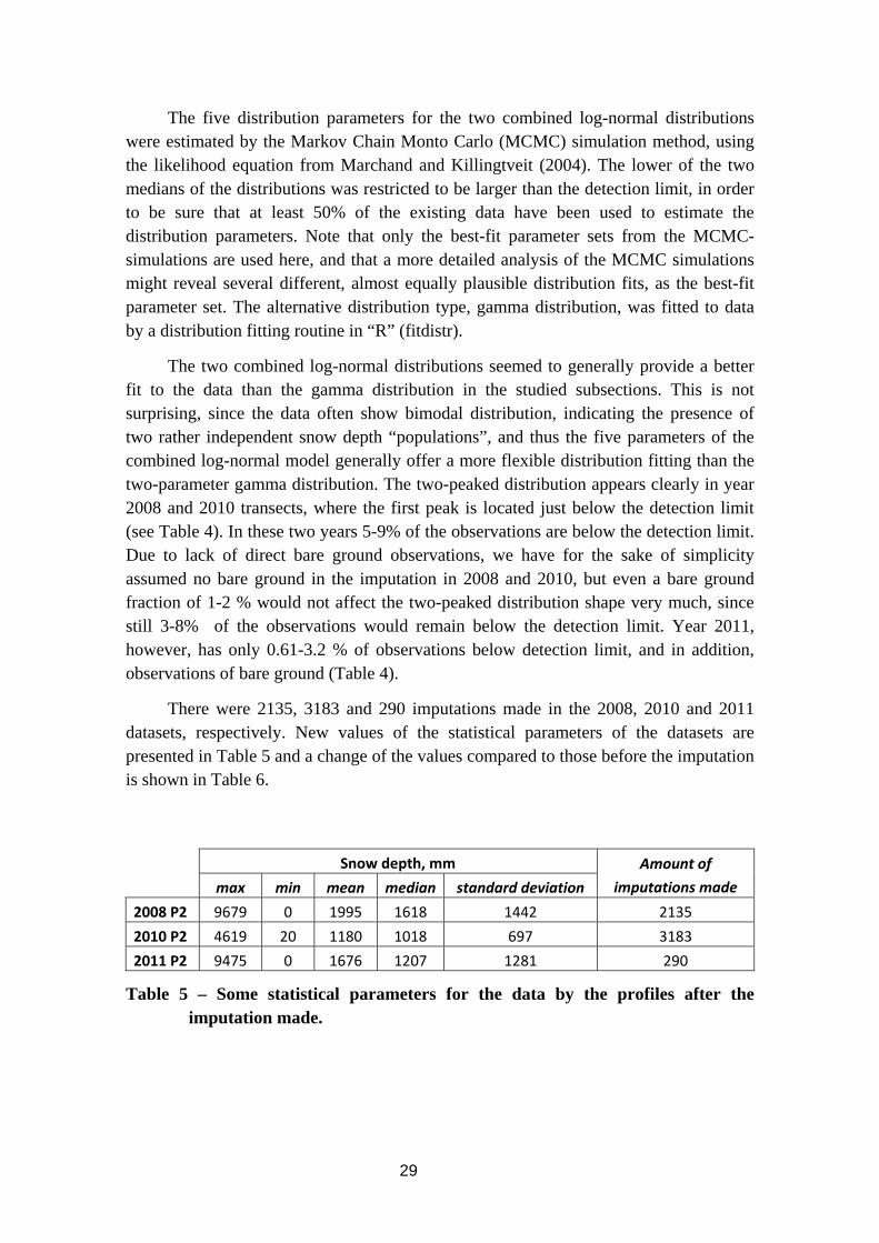
The five distribution parameters for the two combined log-normal distributions were estimated by the Markov Chain Monto Carlo (MCMC) simulation method, using the likelihood equation from Marchand and Killingtveit (2004). The lower of the two medians of the distributions was restricted to be larger than the detection limit, in order to be sure that at least 50% of the existing data have been used to estimate the distribution parameters. Note that only the best-fit parameter sets from the MCMC-simulations are used here, and that a more detailed analysis of the MCMC simulations might reveal several different, almost equally plausible distribution fits, as the best-fit parameter set. The alternative distribution type, gamma distribution, was fitted to data by a distribution fitting routine in “R” (fitdistr).

The two combined log-normal distributions seemed to generally provide a better fit to the data than the gamma distribution in the studied subsections. This is not surprising, since the data often show bimodal distribution, indicating the presence of two rather independent snow depth “populations”, and thus the five parameters of the combined log-normal model generally offer a more flexible distribution fitting than the two-parameter gamma distribution. The two-peaked distribution appears clearly in year 2008 and 2010 transects, where the first peak is located just below the detection limit (see Table 4). In these two years 5-9% of the observations are below the detection limit. Due to lack of direct bare ground observations, we have for the sake of simplicity assumed no bare ground in the imputation in 2008 and 2010, but even a bare ground fraction of 1-2 % would not affect the two-peaked distribution shape very much, since still 3-8% of the observations would remain below the detection limit. Year 2011, however, has only 0.61-3.2 % of observations below detection limit, and in addition, observations of bare ground (Table 4).

There were 2135, 3183 and 290 imputations made in the 2008, 2010 and 2011 datasets, respectively. New values of the statistical parameters of the datasets are presented in Table 5 and a change of the values compared to those before the imputation is shown in Table 6.

Snow depth, mm  Amount of 

imputations made max  min  mean  median standard deviation 

2008 P2  9679  0  1995  1618  1442  2135 

2010 P2  4619  20  1180  1018  697  3183 

2011 P2  9475  0  1676  1207  1281  290 

Table 5 – Some statistical parameters for the data by the profiles after the imputation made.

30

Snow depth, mm 

max  min  mean  median  Amount of imputations made 

2008 P2  0  ‐259  ‐118  ‐70  2135 

2010 P2  0  ‐298  ‐86  ‐49  3183 

2011 P2  0  0  ‐7 ‐2 290 

Table 6 – Change in statistical parameters after the imputation made.

31

Conclusions The GPR profiling method reproduces snow depth measurements on

Hardangervidda very well when the data are calibrated with manual snow depth measurements. However, the technical limitations of snow radar make it not only useful but essential to perform snow free tick-marks during field surveys. Such marks will help correct digitalisation and estimation of snow free areas.

Unfortunately, even that is not enough to get a complete set of trustworthy data. The problem to interpret snow thickness in the range of 1-25 cm (between the DL and snow-free area) will still remain. In order to fill these gaps in the dataset a statistical imputation method can be used to simulate values and thereby improve the statistical computation.

We found large spatial variations in snow depth along latitudinal (west – east) profiles with a general tendency of both decreasing accumulation and less variation towards the east for all the years with measurements.

Comparison between our snow depth measurements and the SeNorge snow model estimates showed roughly 50% overestimation of the snow depth simulated by the model.

Most of the constructed snow depth distributions have a two-peak shape. Although the GPR-data from open field sites in Marchand and Killingtveit (2005) showed a similar two-peak structure as seen in most of our transects, it remains unclear whether the secondary peak is a real feature, that is a significantly low snow depth population or a large bare ground fraction, or merely an artefact of the radar data. A closer investigation of this issue could improve our knowledge of the nature of snow depth distribution in mountain plateaus, and of the sampling and interpretation of radar-based snow measurements.

32

References Borgstrøm, R., 2001. Relationship between spring snow depth and growth of Brown

Trout, Salmo trutta, in an alpine lake: Predicting consequences of climate change. Arctic, Antarctic, and Alpine Research 33: 476-480

Cleveland, W.S., 1979. "Robust Locally Weighted Regression and Smoothing Scatterplots". Journal of the American Statistical Association 74 (368): 829–836.

Engeset, R., Tveito, O. E., Udnæs, H-C., Alfnes, E., Mengistu, Z., Isaksen, K. and Førland, E. J., 2004. Snow map validation for Norway. XXIII Nordic Hydrological Conference, 8-12 Aug. 2004, Tallinn, Estonia. NHP report 48(1): 122-131. http://senorge.no/senorgeAux/NHC2004Tallinn_SnowMapValidation_Paper.pdf

Hamran, S.-E., 1996. Radar in glaciology, Lecture notes, University Centre in Svalbard (UNIS), Longyearbyen, Svalbard

Kovacs, A., Gow, A.J. and Morey, R.M., 1995. The in-situ dielectric constant of polar firn revisited. Cold Regions Science and Technology 23 (3), 245-256.

Marchand, W.-D. and Killingtveit, Å., 2004. Statistical properties of spatial snowcover in mountainous catchments in Norway. Nordic Hydrology 35, 101-117.

Marchand, W.-D. and Killingtveit, Å., 2005. Statistical probability distributions of snow depth at the model sub-grid cell spatial scale. Hydrological Processes, 19, 355-369.

Odland, A. and Munkejord, H.K., 2008. Plants as indicators of snow layer duration in southern Norway mountains. Ecological Indicators 8, 57-68.

Saloranta, T., 2011 (manuscript in preparation). Sensitivity analysis and MCMC calibration of the seNorge snow model.

Stand, O., Bevanger, K. and Falldorf, T., 2006. Villreinens bruk av Hardangervidda. Sluttrapport fra Rv7-prosjekt. NINA Rapport 131, 67s.

Stranden, H. B., 2010. Evaluering av seNorge. Data versjon 1.1. Dokument nr. 4/2010, Norges vassdrags- og energidirektorat (NVE). In Norwegian.

This series is published by Norwegian Water Resources and Energy Directorate (NVE)

Published in the Report series 2011 Nr. 1 Representation of catchment hydrology, water balance, runoff and discharge in the JULES and SURFEX land surface models. Tuomo Saloranta (26 s.)

Nr. 2 Mapping of selected markets with Nodal pricing or similar systems Australia, New Zealand and North American power markets. Vivi Mathiesen (Ed.) (44 s.)

Nr. 3 Glaciological investigations in Norway in 2010: Bjarne Kjøllmoen (Ed.) (99 s.) Nr. 4 Climate change impacts on the flow regimes of rivers in Bhutan and possible consequences for hydropower development. Stein Beldring (Ed.) (153 s.)

Nr. 5 Hydrological projections for floods in Norway under a future climate. Deborah Lawrenc, Hege Hisdal (47 s.)

Nr. 6 Project report for the project Hydrological Flood Forecasting System for Small and Medium Sized Catchments in Serbia, 2009 – 2010. Documentation and technical references. Elin Langsholt (57s.)

Nr. 7 Preliminary Flood Risk Assessment in Norway. An example of a methodology based on a GIS-approach (39 s.)

Nr. 8 GPR-measurements of snow distribution on Hardangervidda mountain plateau in 2008-2011, Galina Ragulina, Kjetil Melvold, Tuomo Saloranta (32 s.)

Norwegian Water Resources and Energy Directorate

Middelthunsgate 29 PB. 5091 Majorstuen N-0301 Oslo Norway

Telephone: +47 09575Internet: www.nve.no