GPM precipitation feature database

Description Version 1.0

Chuntao Liu

Department of Physical and Environmental Sciences Texas A&M University at Corpus Christi

6300 Ocean Dr., Corpus Christi, TX, 78412-5850

(o) 361-825-3845

(fax) 361-825-3355

chuntao.liu@tamucc.edu

http://atmos.tamucc.edu/trmm/

2016. 01

Table of content 1. Introduction 2. Level-1

2.1 Collocation between 1B-GMI and Ku, Ka, and DPR 2.2 Parallax correction 2.3 Collocation after Parallax correction

2.4 Output parameters

3. Level-2 3.1 Definitions 3.2 Parameters 3.3 Parameters from ERA-Interim analysis

4. Level-3

5. References 6. Appendix

A. Website and acess B. Reading software

1. Introduction

The Global Precipitation Mission (GPM, Hou et al., 2014) is a joint mission between NASA and the National Space Development Agency (NASDA) of Japan designed to monitor and study global precipitation. Onboard instruments including Dual frequency Precipitation Radar (DPR) and GPM Microwave Imager (GMI) provide invaluable measurements of precipitation and atmosphere.

One direction of our research is to generalize the Precipitation Features (PFs) from satellite measurements and study the radar and passive microwave characteristics of precipitating systems on Earth. The idea of PF was first introduced in late 1990s by using the passive microwave brightness temperature observations from SSMI satellites (Mohr and Zipser, 1996). Later, using observations from Tropical Rainfall Measuring Mission (Kummerow et al. 1998), a more descriptive database was created (Nesbitt et al. 2000) and then upgraded (Liu et al. 2008). The TRMM PF database has been widely used in scientific research, including rainfall estimates validation (Nesbitts et al., 2004), diurnal cycle of precipitation systems (Nesbitt and Zipser, 2003), global distribution of storms with LIS-detected lightning (Cecil et al., 2005), deep convection reaching the tropical tropopause layer (Liu and Zipser, 2005), rainfall production and convective organization (Nesbitt et al. 2006), and the categorization of extreme thunderstorms by their intensity proxies (Zipser et al., 2006) etc. Current version of TRMM PF database is the newest development based on the TRMM product version 7 that reprocessed in 2012. Following the same research track, a similar database from GPM observations has been built.

After the successful launch in February 2014, GPM satellite has been collecting observations globally. Following the heritage of the TRMM PF database, the GPM precipitation feature database has been developed at Texas A&M –Corpus Christi in collaboration with Dr. Zipser at the University of Utah and Dr. Cecil at NASA MSFC. This database includes GPM DPR and GMI precipitation estimates and radar vertical structure inside and outside the DPR swath in precipitation features. This document describes the GPM precipitation database construction procedures and output parameters in two levels of processing as shown in Figure 1.

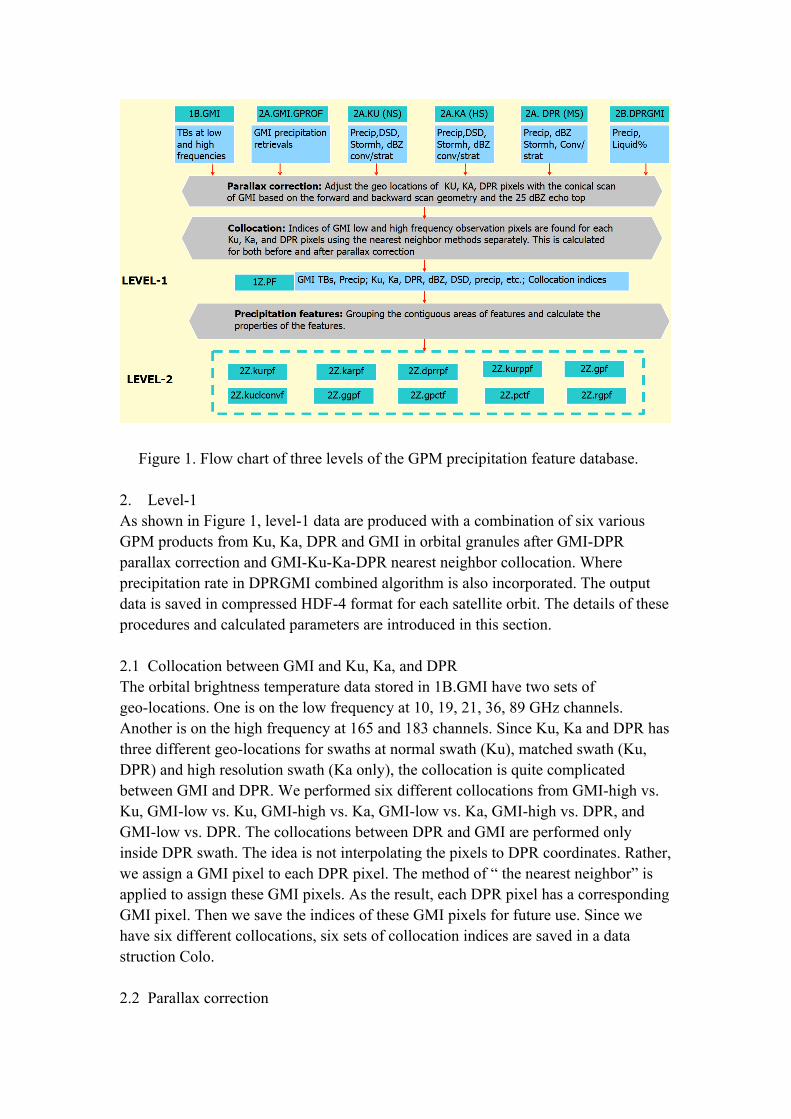
Figure 1. Flow chart of three levels of the GPM precipitation feature database. 2. Level-1 As shown in Figure 1, level-1 data are produced with a combination of six various GPM products from Ku, Ka, DPR and GMI in orbital granules after GMI-DPR parallax correction and GMI-Ku-Ka-DPR nearest neighbor collocation. Where precipitation rate in DPRGMI combined algorithm is also incorporated. The output data is saved in compressed HDF-4 format for each satellite orbit. The details of these procedures and calculated parameters are introduced in this section. 2.1 Collocation between GMI and Ku, Ka, and DPR The orbital brightness temperature data stored in 1B.GMI have two sets of geo-locations. One is on the low frequency at 10, 19, 21, 36, 89 GHz channels. Another is on the high frequency at 165 and 183 channels. Since Ku, Ka and DPR has three different geo-locations for swaths at normal swath (Ku), matched swath (Ku, DPR) and high resolution swath (Ka only), the collocation is quite complicated between GMI and DPR. We performed six different collocations from GMI-high vs. Ku, GMI-low vs. Ku, GMI-high vs. Ka, GMI-low vs. Ka, GMI-high vs. DPR, and GMI-low vs. DPR. The collocations between DPR and GMI are performed only inside DPR swath. The idea is not interpolating the pixels to DPR coordinates. Rather, we assign a GMI pixel to each DPR pixel. The method of “ the nearest neighbor” is applied to assign these GMI pixels. As the result, each DPR pixel has a corresponding GMI pixel. Then we save the indices of these GMI pixels for future use. Since we have six different collocations, six sets of collocation indices are saved in a data struction Colo. 2.2 Parallax correction

Because GMI scans with 52o conical angle and DPR scans nadir, there could be a problem if the microwave scattering signals are from elevated hydrometeors, such as high convective cells. For this reason, in the past approach (before 2008), we used a simple parallax correction method that simply move the GMI data coordinates data backwards for one scan shown as Figure 2. After this correction, there are better correspondences between DPR and GMI measurements for high convective cells. However, the correspondences between DPR and GMI for shallow precipitations become worse because of the overcorrection. This could lead to problems when calculate the microwave scattering properties inside a shallow precipitation system defined by DPR surface precipitation area. So in the current version, the parallax correction only made for the pixels with DPR ku echo top height > 5 km and path integrated attenuation > 0.4 dBZ. In this way, the overcorrection for the shallow precipitations is avoided.

Figure 2. Schematic diagram of parallax correction for TRMM. The similar scenario applies for GPM DPR and GMI as well. 2.3 Re-collocation after the parallax correction After the parallax correction, we redo the collocation to make the matching between passive microwave and radar more realistic. To make this flexible to the users, current version includes both collocation indices before and after the parallax correction. 2.4 Output parameters We have chosen some interesting parameters from 1B.GMI, 2A.GMI, 2A.DPR, 2A.Ku, 2A.Ka, 2B.DPRGMI, and some derived parameters for storing into the level-1

products. These parameters include: Parameters from 1B.GMI and 2A.GMI LAT FLOAT Array[221, 2961] Latitude of low freq TBs LON FLOAT Array[221, 2961] Longitude of low freq TBs TB FLOAT Array[9, 221, 2961] TBs at low frequency DAY BYTE Array[2961] Day HOUR BYTE Array[2961] Hour MINUTE BYTE Array[2961] Minute MONTH BYTE Array[2961] Month SECOND BYTE Array[2961] Second YEAR INT Array[2961] YEAR ORIENT INT Array[2961] Orientation QUALITY BYTE Array[2961] Quality of TBs HITB FLOAT Array[4, 221, 2961] High frequency TBs HIQUALITY BYTE Array[2961] Quality of high freq TBs HILAT FLOAT Array[221, 2961] Latitude of high freq TBs HILON FLOAT Array[221, 2961] Longitude of high freq TBs PCT85 FLOAT Array[221, 2961] Polarization Corrected 89 GHz PCT37 FLOAT Array[221, 2961] Polarization correction 37 GHz PRECIP FLOAT Array[221, 2961] Surface precipitation retrieval FRLIQ FLOAT Array[221, 2961] Fraction of liquid PROB FLOAT Array[221, 2961] Probability of Precip IWP FLOAT Array[221, 2961] Ice water Path RWP FLOAT Array[221, 2961] Rain water path CWP FLOAT Array[221, 2961] Cloud water path FRCONV FLOAT Array[221, 2961] Convective fraction SFCTYPE BYTE Array[221, 2961] Surface type MLPRECIP FLOAT Array[221, 2961] Melting level Precip RETRQUAL BYTE Array[221, 2961] retrieval quality

Parameters from 2A.Ku LAT FLOAT Array[49, 7930] Latitude LON FLOAT Array[49, 7930] Longitude PRECIPTYPE LONG Array[49, 7930] Precipitation type STORMHT FLOAT Array[49, 7930] Echo top height DSD FLOAT Array[2, 176, 49, 7930] DSD parameter PHASE BYTE Array[49, 7930] Phase PIA FLOAT Array[49, 7930] Path integrated attenuation PRECIP FLOAT Array[176, 49, 7930] Precipitation retrievals ESPRECIP FLOAT Array[49, 7930] Estimated surface precip NSPRECIP FLOAT Array[49, 7930] Near surface precip DBZ FLOAT Array[176, 49, 7930] Reflectivity profiles

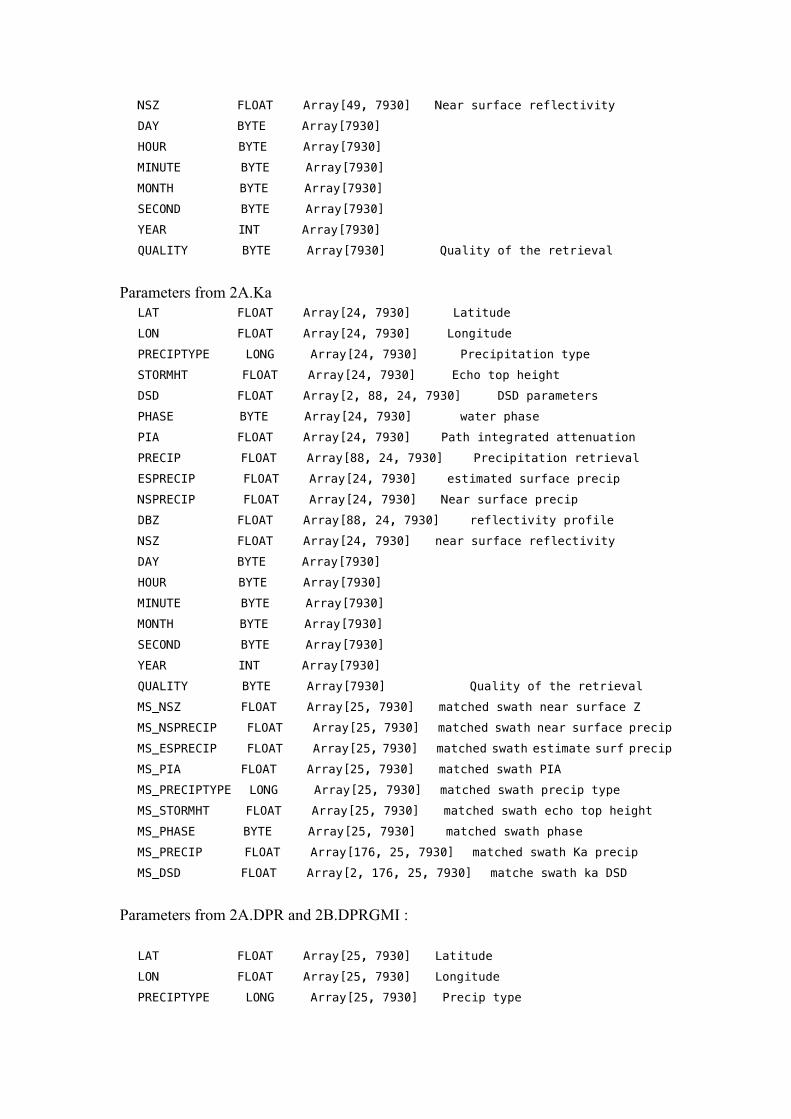
NSZ FLOAT Array[49, 7930] Near surface reflectivity DAY BYTE Array[7930] HOUR BYTE Array[7930] MINUTE BYTE Array[7930] MONTH BYTE Array[7930] SECOND BYTE Array[7930] YEAR INT Array[7930] QUALITY BYTE Array[7930] Quality of the retrieval

Parameters from 2A.Ka LAT FLOAT Array[24, 7930] Latitude LON FLOAT Array[24, 7930] Longitude PRECIPTYPE LONG Array[24, 7930] Precipitation type STORMHT FLOAT Array[24, 7930] Echo top height DSD FLOAT Array[2, 88, 24, 7930] DSD parameters PHASE BYTE Array[24, 7930] water phase PIA FLOAT Array[24, 7930] Path integrated attenuation PRECIP FLOAT Array[88, 24, 7930] Precipitation retrieval ESPRECIP FLOAT Array[24, 7930] estimated surface precip NSPRECIP FLOAT Array[24, 7930] Near surface precip DBZ FLOAT Array[88, 24, 7930] reflectivity profile NSZ FLOAT Array[24, 7930] near surface reflectivity DAY BYTE Array[7930] HOUR BYTE Array[7930] MINUTE BYTE Array[7930] MONTH BYTE Array[7930] SECOND BYTE Array[7930] YEAR INT Array[7930] QUALITY BYTE Array[7930] Quality of the retrieval MS_NSZ FLOAT Array[25, 7930] matched swath near surface Z MS_NSPRECIP FLOAT Array[25, 7930] matched swath near surface precip MS_ESPRECIP FLOAT Array[25, 7930] matched swath estimate surf precip MS_PIA FLOAT Array[25, 7930] matched swath PIA MS_PRECIPTYPE LONG Array[25, 7930] matched swath precip type MS_STORMHT FLOAT Array[25, 7930] matched swath echo top height MS_PHASE BYTE Array[25, 7930] matched swath phase MS_PRECIP FLOAT Array[176, 25, 7930] matched swath Ka precip MS_DSD FLOAT Array[2, 176, 25, 7930] matche swath ka DSD

Parameters from 2A.DPR and 2B.DPRGMI : LAT FLOAT Array[25, 7930] Latitude LON FLOAT Array[25, 7930] Longitude PRECIPTYPE LONG Array[25, 7930] Precip type

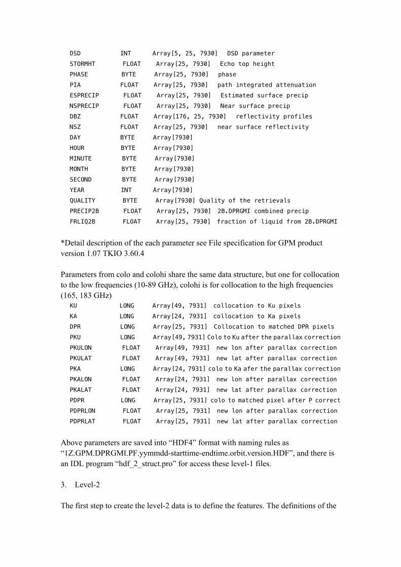
DSD INT Array[5, 25, 7930] DSD parameter STORMHT FLOAT Array[25, 7930] Echo top height PHASE BYTE Array[25, 7930] phase PIA FLOAT Array[25, 7930] path integrated attenuation ESPRECIP FLOAT Array[25, 7930] Estimated surface precip NSPRECIP FLOAT Array[25, 7930] Near surface precip DBZ FLOAT Array[176, 25, 7930] reflectivity profiles NSZ FLOAT Array[25, 7930] near surface reflectivity DAY BYTE Array[7930] HOUR BYTE Array[7930] MINUTE BYTE Array[7930] MONTH BYTE Array[7930] SECOND BYTE Array[7930] YEAR INT Array[7930] QUALITY BYTE Array[7930] Quality of the retrievals PRECIP2B FLOAT Array[25, 7930] 2B.DPRGMI combined precip FRLIQ2B FLOAT Array[25, 7930] fraction of liquid from 2B.DPRGMI

*Detail description of the each parameter see File specification for GPM product version 1.07 TKIO 3.60.4 Parameters from colo and colohi share the same data structure, but one for collocation to the low frequencies (10-89 GHz), colohi is for collocation to the high frequencies (165, 183 GHz) KU LONG Array[49, 7931] collocation to Ku pixels KA LONG Array[24, 7931] collocation to Ka pixels DPR LONG Array[25, 7931] Collocation to matched DPR pixels PKU LONG Array[49, 7931] Colo to Ku after the parallax correction PKULON FLOAT Array[49, 7931] new lon after parallax correction PKULAT FLOAT Array[49, 7931] new lat after parallax correction PKA LONG Array[24, 7931] colo to Ka afer the parallax correction PKALON FLOAT Array[24, 7931] new lon after parallax correction PKALAT FLOAT Array[24, 7931] new lat after parallax correction PDPR LONG Array[25, 7931] colo to matched pixel after P correct PDPRLON FLOAT Array[25, 7931] new lon after parallax correction PDPRLAT FLOAT Array[25, 7931] new lat after parallax correction

Above parameters are saved into “HDF4” format with naming rules as “1Z.GPM.DPRGMI.PF.yymmdd-starttime-endtime.orbit.version.HDF”, and there is an IDL program “hdf_2_struct.pro” for access these level-1 files. 3. Level-2 The first step to create the level-2 data is to define the features. The definitions of the

precipitation features are either based on the DPR swath or GMI swath (Figure 2).

Figure 2. Definitions of GPM precipitation features 3.1 Definitions Figure 2 lists current precipitation feature definitions. Kurpf, Karpf, and DPRrpf are defined based on the contiguous pixels with non zero precipitation rate (here > 0.1mm/hr is used) from Ku, Ka, and DPR retrievals. Kurppf is based on the projected area with any radar echo in the column. gpf is based on the GMI precipitation inside Ku swath. Rgpf and kuclconf are designed to assess the performance of retrievals and the convective regions for storms. Ggpf is the GMI precipitation feature in GMI swath. Gpctf is defined with area of GMI 89GHz Polarization Corrected Temperature (PCT, Spence et al., 1989) colder than 250 K. 3.2 Parameters After grouping the pixels with different criteria, the indices of pixels for each feature are identified within PF swath from collocated level-1 data. Using these indices, the total number of pixels, maximum echo tops, and minimum brightness temperatures inside features are calculated and saved as level-2 product.

The parameters for each feature in level-2 product are listed below:

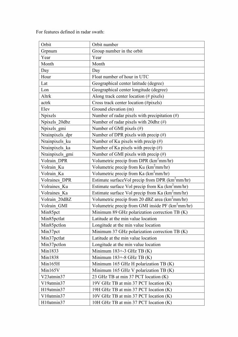
For features defined in radar swath:

Orbit Orbit number Grpnum Group number in the orbit Year Year Month Month Day Day Hour Float number of hour in UTC Lat Geographical center latitude (degree) Lon Geographical center longitude (degree) Altrk Along track center location (# pixels) actrk Cross track center location (#pixels) Elev Ground elevation (m) Npixels Number of radar pixels with precipitation (#) Npixels_20dbz Number of radar pixels with 20dbz (#) Npixels_gmi Number of GMI pixels (#) Nrainpixels_dpr Number of DPR pixels with precip (#) Nrainpixels_ku Number of Ku pixels with precip (#) Nrainpixels_ka Number of Ka pixels with precip (#) Nrainpixels_gmi Number of GMI pixels with precip (#) Volrain_DPR Volumetric precip from DPR (km2mm/hr) Volrain_Ku Volumetric precip from Ku (km2mm/hr) Volrain_Ka Volumetric precip from Ka (km2mm/hr) Volraines_DPR Estimate surfaceVol precip from DPR (km2mm/hr) Volraines_Ku Estimate surface Vol precip from Ku (km2mm/hr) Volraines_Ka Estimate surface Vol precip from Ka (km2mm/hr) Volrain_20dBZ Volumetric precip from 20 dBZ area (km2mm/hr) Volrain_GMI Volumetric precip from GMI inside PF (km2mm/hr) Min85pct Minimum 89 GHz polarization correction TB (K) Min85pctlat Latitude at the min value location Min85pctlon Longitude at the min value location Min37pct Minimum 37 GHz polarization correction TB (K) Min37pctlat Latitude at the min value location Min37pctlon Longitude at the min value location Min1833 Minimum 183+-3 GHz TB (K) Min1838 Minimum 183+-8 GHz TB (K) Min165H Minimum 165 GHz H polarization TB (K) Min165V Minimum 165 GHz V polarization TB (K) V23atmin37 23 GHz TB at min 37 PCT location (K) V19atmin37 19V GHz TB at min 37 PCT location (K) H19atmin37 19H GHz TB at min 37 PCT location (K) V10atmin37 10V GHz TB at min 37 PCT location (K) H10atmin37 10H GHz TB at min 37 PCT location (K)

Nlt275 Number of radar pixels with 89 GHz PCT < 275 K (#) Nlt250 Number of radar pixels with 89 GHz PCT < 250 K (#) Nlt225 Number of radar pixels with 89 GHz PCT < 225 K (#) Nlt200 Number of radar pixels with 89 GHz PCT < 200 K (#) Nlt175 Number of radar pixels with 89 GHz PCT < 175 K (#) Nlt150 Number of radar pixels with 89 GHz PCT < 150 K (#) Nlt125 Number of radar pixels with 89 GHz PCT < 125 K (#) Nlt100 Number of radar pixels with 89 GHz PCT < 100 K (#) Maxnsz Maximum near surface reflectivity (dBZ) Maxnsprecip Maximum near surface precip rate (mm/hr) Maxnsz_Ku Maximum Ku near surface reflectivity (dBZ) Maxnsz_Ka Maximum Ka near surface reflectivity (dBZ) Maxnsprecip_Ku Maximum Ku near surface precip rate (mm/hr) Maxnsprecip_Ka Maximum Ka near surface precip rate (mm/hr) Maxnsz_lon Longitude of location with maximum NSZ Maxnsz_lat Latitude of location with maximum NSZ N20dbz Profile of number of 20 dBZ in PF (#) N25dbz Profile of number of 25 dBZ in PF (#) N30dbz Profile of number of 30 dBZ in PF (#) N35dbz Profile of number of 35 dBZ in PF (#) N40dbz Profile of number of 40 dBZ in PF (#) N45dbz Profile of number of 45 dBZ in PF (#) N50dbz Profile of number of 50 dBZ in PF (#) Maxdbz Profile of Maximum reflectivity (dBZ) Maxht Maximum height with 15 dBZ echo (km) Maxhtlon Longitude of maxht location Maxhtlat Latitude of maxht location Maxht15 Maximum height with 15 dBZ echo (km) Maxht20 Maximum height with 20 dBZ echo (km) Maxht20lon Longitude of maxht20 location Maxht20lat Latitude of maxht20 location Maxht30 Maximum height with 30 dBZ echo (km) Maxht30lon Longitude of maxht 30 location Maxht30lat Latitude of maxht30 location Maxht40 Maximum height with 40 dBZ echo (km) Maxht40lon Longitude of maxht40 location Maxht40lat Latitude of maxht40 location Landocean 0: over ocean. 1: over land Nstrat_dpr Number of pixels with stratiform rainfall (#) Nconv_dpr Number of pixels with convective rainfall (#) Rainstrat_dpr Stratiform volumetric rain (km2mm/hr) Rainconv_dpr Convective volumetric rain (km2mm/hr) Nstrat_ku Number of pixels with stratiform rainfall (#)

Nconv_ku Number of pixels with convective rainfall (#) Rainstrat_ku Stratiform volumetric rain (km2mm/hr) Rainconv_ku Convective volumetric rain (km2mm/hr) Nstrat_ka Number of pixels with stratiform rainfall (#) Nconv_ka Number of pixels with convective rainfall (#) Rainstrat_ka Stratiform volumetric rain (km2mm/hr) Rainconv_ka Convective volumetric rain (km2mm/hr) R_lon* Center location longitude of fitted ellipse R_lat Center location latitude of fitted ellipse R_major Major axis of ellipsis (km) R_minor Minor axis of ellipsis (km) R_orientation Orientation angle (degree) R_solid Percentage filled by rainfall area

The morphology of the feature can be represented by major, minor axes, orientation angle of fitted ellipse. Here R_xxx are the parameters fitted for whole feature

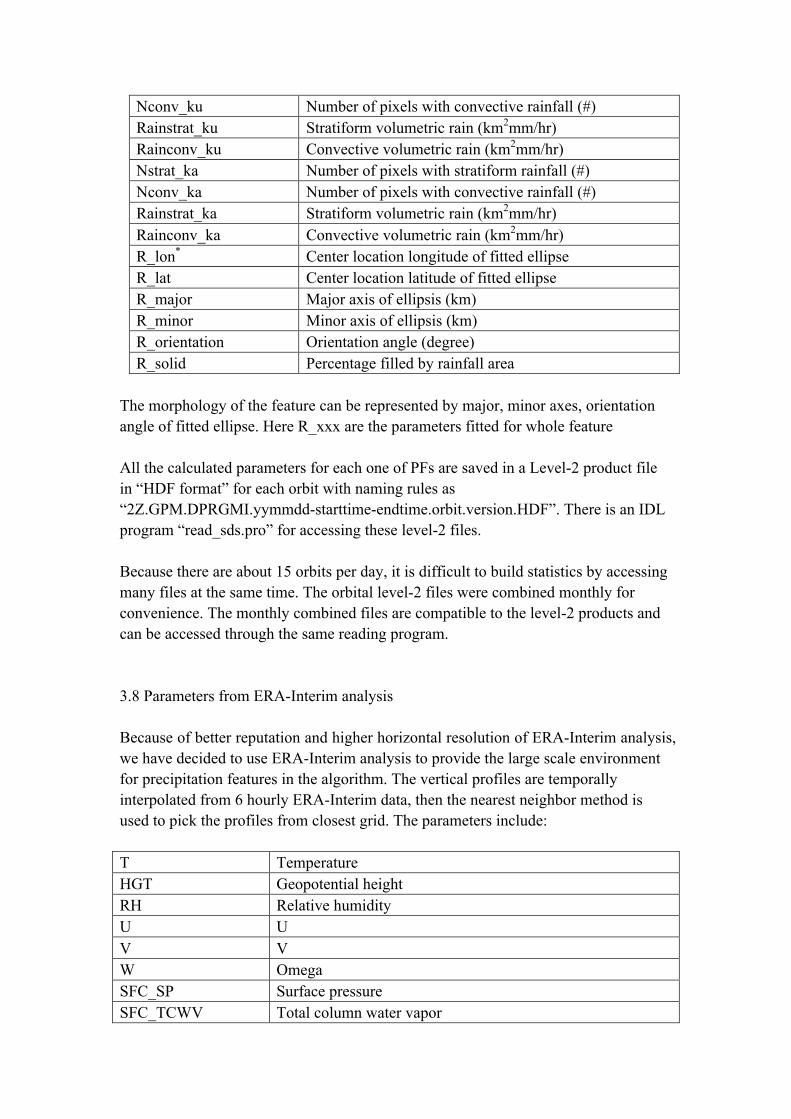
All the calculated parameters for each one of PFs are saved in a Level-2 product file in “HDF format” for each orbit with naming rules as “2Z.GPM.DPRGMI.yymmdd-starttime-endtime.orbit.version.HDF”. There is an IDL program “read_sds.pro” for accessing these level-2 files. Because there are about 15 orbits per day, it is difficult to build statistics by accessing many files at the same time. The orbital level-2 files were combined monthly for convenience. The monthly combined files are compatible to the level-2 products and can be accessed through the same reading program. 3.8 Parameters from ERA-Interim analysis Because of better reputation and higher horizontal resolution of ERA-Interim analysis, we have decided to use ERA-Interim analysis to provide the large scale environment for precipitation features in the algorithm. The vertical profiles are temporally interpolated from 6 hourly ERA-Interim data, then the nearest neighbor method is used to pick the profiles from closest grid. The parameters include: T Temperature HGT Geopotential height RH Relative humidity U U V V W Omega SFC_SP Surface pressure SFC_TCWV Total column water vapor

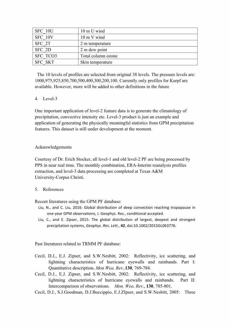
SFC_10U 10 m U wind SFC_10V 10 m V wind SFC_2T 2 m temperature SFC_2D 2 m dew point SFC_TCO3 Total column ozone SFC_SKT Skin temperature The 10 levels of profiles are selected from original 38 levels. The pressure levels are: 1000,975,925,850,700,500,400,300,200,100. Currently only profiles for Kurpf are available. However, more will be added to other definitions in the future 4. Level-3 One important application of level-2 feature data is to generate the climatology of precipitation, convective intensity etc. Level-3 product is just an example and application of generating the physically meaningful statistics from GPM precipitation features. This dataset is still under development at the moment. Acknowledgements Courtesy of Dr. Erich Stocker, all level-1 and old level-2 PF are being processed by PPS in near real time. The monthly combination, ERA-Interim reanalysis profiles extraction, and level-3 data processing are completed at Texas A&M University-Corpus Christi. 5. References Recent literatures using the GPM PF database: Liu,   N.,   and   C.   Liu,   2016:   Global   distribution   of   deep   convection   reaching   tropopause   in  

one-­‐year  GPM  observations,  J.  Geophys.  Res.,  conditional  accepted.  Liu,   C.,   and   E.   Zipser,   2015:   The   global   distribution   of   largest,   deepest   and   strongest  

precipitation  systems,  Geophys.  Res.  Lett.,  42,  doi:10.1002/2015GL063776.     Past literatures related to TRMM PF database: Cecil, D.J., E.J. Zipser, and S.W.Nesbitt, 2002: Reflectivity, ice scattering, and

lightning characteristics of hurricane eyewalls and rainbands. Part I: Quantitative description. Mon Wea. Rev.,130, 769-784.

Cecil, D.J., E.J. Zipser, and S.W.Nesbitt, 2002: Reflectivity, ice scattering, and lightning characteristics of hurricane eyewalls and rainbands. Part II: Intercomparison of observations. Mon. Wea. Rev., 130, 785-801.

Cecil, D.J., S.J.Goodman, D.J.Boccippio, E.J.ZIpser, and S.W.Nesbitt, 2005: Three

years of TRMM precipitation features. Part 1: Radar, radiometric, and lightning characteristics. Mon Wea. Rev., 133, 543-566.

Huffman, G., R. Adler, M. Morrissey, D. Bolvin, S. Cuttis, R. Joyce, B. McGavock and J.Susskind, 2001: Global precipitation at one degree resolution from multi satellite observations. J. Hydrometeor., 2, 36-50.

Iguchi, T., T. Kozu., R. Meneghini, J. Awaka, and K. Okamoto, 2000: Rain-profiling algorithm for the TRMM precipitation radar. J. Appl. Meteor., 39, 2038-2052.

Joyce, R., and P. A. Arkin, 1997: Improved estimates of tropical and subtropical precipitation using the GOES Precipitation Index. J. Atmos. Ocean. Tech., 10, 997-1011.

Kistler, R., E. Kalnay, W. Collins, S. Saha, G. White, J. Woollen, M. Chelliah, W. bisuzaki, M. Kanamitsu, V. Kousky, H. Dool, R. Jenne and M. Fiorino, 2001: The NCEP-NCAR 5—year reanalysis: monthly means CD-ROM and documentation. Bull. Amer. Meteor. Soc. 82, 247-267.

Kummerow, C., W. Barnes, T. Kozu, J. Shiue, and J. Simpson, 1998: The Tropical Rainfall Measuring Mission (TRMM) sensor package. J. Atmos. Oceanic Tech., 15, 809–817.

Kummerow, C., 23 coauthors, and E. J. Zipser, 2000: The status of the Tropical Rain Measuring Mission (TRMM) after 2 years in orbit. J. Appl. Meteor., 39, 1965-1982

Liu, C. and E.J. Zipser, 2005: Global distribution of convection penetrating the tropical tropopause. J.Geophys. Res.-Atm, 110, doi:10.1029/2005JD00006063.

Liu, C., E,J,Zipser, and S.W.Nesbitt, 2007: Global distribution of tropical deep convection: Differences using infrared and radar as the primary data source. J. Climate, 20, 489-503, DOI:10.1175/JCLI4023.1.

Nesbitt, S.W., E. J. Zipser, and D.J. Cecil, 2000: A census of precipitation features in the tropics using TRMM: Radar, ice scattering, and lightning observations. J. Climate, 13 (23), 4087-4106

Nesbitt, S.W., and E.J.Zipser, 2003: The diurnal cycle of rainfall and convective intensity according to three years of TRMM measurements. J. Climate, 16 (10), 1456-1475

Nesbitt, S.W., E.J. Zipser, and C.D. Kummerow, 2004: An examination of Version-5 rainfall estimates from the TRMM Microwave Imager, Precipitation Radar, and rain gauges on global, regional, and storm scales. J. Appl. Meteor., 43, 1016-1036.

Rudolf, B., 1993: Management and analysis of precipitation data on a routine basis. Proc. Int. WMO/IAHS/ETH Symp. on Precipitation and Evaporation, Bratislava, Slovakia, Slovak Hydromet. Inst., 69–76

Spencer, R. W., H. G. Goodman, and R. E. Hood, 1989: Precipitation retrieval over land and ocean with the SSM/I: identification and characteristics of the scattering signal. J. Atmos. Oceanic Tech., 6, 254-273.

Zipser, E.J., D.J.Cecil, C.Liu, S.W.Nesbitt. and D.P.Yorty, 2006: Where are the most intense thunderstorms on earth? Bull, Amer. Meteor. Soc., 87,

1057-1071. 6. Appendix

A. Website and access There is an old website providing access the level-2 products of TRMM databse during 1998-2014 http://trmm.chpc.utah.edu/ A new website has been built and provides access to all the dataset described above. http://atmos.tamucc.edu/trmm/ All TRMM and GMP PF data are available at: http://atmos.tamucc.edu/trmm/data/

B. Reading programs hdf_2_struct.pro This program reads Level-1 GPM PF data. Usage: IDL > hdf_2_struct,’1Z.GPM.DPRGMI.xxxxxxxxx.xxxxxx.x.HDF’,f Here f is a structure storing all the level-1 variables.

Read_sds.pro This program reads all the science data from HDF-4 format file and save into a structure. This program can be used to access level-2 products with new definitions and all level-3 products. Usage example: IDL> read_sds,’example.HDF’,f ; f is a structure variable with all the parameters

Read_sds_one.pro This program reads in one variable from HDF-4 format file Usage: IDL> read_sds_one,’example.HDF’,’var1’,var All these IDL programs can be downloaded at: http://atmos.tamucc.edu/trmm/software/