Which estimator to measure local governments’ cost efficiency? An application to Spanish municipalities

Isabel Narbón-Perpiñá Maria Teresa Balaguer-Coll Marko Petrovic Emili Tortosa-Ausina

2017 / 06

Which estimator to measure local governments’ cost

efficiency? An application to Spanish municipalities

2017 / 06

Abstract

We analyse overall cost efficiency in Spanish local governments during the crisis

period (2008–2013). To this end, we first consider some of the most popular

methods to evaluate local government efficiency, DEA (Data Envelopment

Analysis) and FDH (Free Disposal Hull), as well as recent proposals, namely the

order-m partial frontier and the non-parametric estimator proposed by Kneip, Simar

and Wilson (2008), which are also non-parametric approaches. Second, we

compare the methodologies used to measure efficiency. In contrast to previous

literature, which has regularly compared techniques and made proposals for

alternative methodologies, we follow recent proposals (Badunenko et al., 2012)

with the aim of comparing the four methods and choosing the one which performs

best with our particular dataset, that is, the most appropriate method for measuring

local government cost efficiency in Spain. We carry out the experiment via Monte

Carlo simulations and discuss the relative performance of the efficiency scores

under various scenarios. Our results suggest that there is no one approach suitable

for all efficiency analysis. We find that for our sample of 1,574 Spanish local

governments, the average cost efficiency would have been between 0.54 and 0.77

during the period 2008–2013, suggesting that Spanish local governments could

have achieved the same level of local outputs with about 23% to 36% fewer

resources.

Keywords: OR in government, efficiency, local government, nonparametric

frontiers

JEL classification: C14, C15, H70, R15

Isabel Narbón-Perpiñá

Universitat Jaume I

Department of Economics

narbon@uji.es

Marko Petrovic

LEE & Universitat Jaume I

Department of Economics

petrovic@uji.es

Mª Teresa Balaguer-Coll

Universitat Jaume I

Dept of Accounting and Finance

bcoll@uji.es

Emili Tortosa-Ausina

IVIE & Universitat Jaume I

Department of Economics

tortosa@uji.es

Which estimator to measure local governments’ cost

efficiency? An application to Spanish municipalities

Isabel Narbón-Perpiñá∗ Maria Teresa Balaguer-Coll† Marko Petrovic‡

Emili Tortosa-Ausina§

April 8, 2017

Abstract

We analyse overall cost efficiency in Spanish local governments during the crisis period (2008–2013). To this end, we first consider some of the most popular methods to evaluate local governmentefficiency, DEA (Data Envelopment Analysis) and FDH (Free Disposal Hull), as well as recentproposals, namely the order-m partial frontier and the non-parametric estimator proposed by Kneip,Simar and Wilson (2008), which are also non-parametric approaches. Second, we compare themethodologies used to measure efficiency. In contrast to previous literature, which has regularlycompared techniques and made proposals for alternative methodologies, we follow recent proposals(Badunenko et al., 2012) with the aim of comparing the four methods and choosing the one whichperforms best with our particular dataset, that is, the most appropriate method for measuring localgovernment cost efficiency in Spain. We carry out the experiment via Monte Carlo simulationsand discuss the relative performance of the efficiency scores under various scenarios. Our resultssuggest that there is no one approach suitable for all efficiency analysis. We find that for our sampleof 1,574 Spanish local governments, the average cost efficiency would have been between 0.54 and0.77 during the period 2008–2013, suggesting that Spanish local governments could have achievedthe same level of local outputs with about 23% to 36% fewer resources.

Keywords: OR in government, efficiency, local government, nonparametric frontiers

JEL Classification: C14, C15, H70, R15

∗Department of Economics, Universitat Jaume I, Campus del Riu Sec, 12071 Castelló de la Plana, Spain, email:narbon@uji.es

†Department of Finance and Accounting, Universitat Jaume I, Campus del Riu Sec, 12071 Castelló de la Plana,Spain, email: bcoll@uji.es

‡Department of Economics, Universitat Jaume I, Campus del Riu Sec, 12071 Castelló de la Plana, Spain, email:petrovic@uji.es

§Department of Economics, Universitat Jaume I, Campus del Riu Sec, 12071 Castelló de la Plana, Spain, email:tortosa@uji.es

1

1. Introduction

Managing the available resources efficiently at all levels of government (central, regional,

and municipal) is essential, particularly in the scenario of the current international economic

crisis, which still affects several European countries. Given that increasing taxes and deficit

is politically costly (Doumpos and Cohen, 2014), a reasonable way to operate in this context

is to improve economic efficiency (De Witte and Geys, 2011), which in cost terms means that

an entity should produce a particular level of output in the cheapest way. In this setting,

since local regulators must provide the best possible local services at the lowest possible cost,

developing a system for evaluating local government performance that allows benchmarks

to be set over time could have relevant practical implications (Da Cruz and Marques, 2014).

However, measuring the performance of local governments is usually highly complex.

Local government efficiency has attracted much scholarly interest in the field of public

administration and there is now a large body of literature covering several countries, such

as Balaguer-Coll et al. (2007) in Spain, Geys et al. (2013) in Germany or Štastná and Gregor

(2015) in the Czech Republic, among others.1 However, despite the high number of empirical

contributions, a major challenge to analysis of local government performance is the lack of

clear, standard methodology to perform efficiency analysis. This is not a trivial question

as much previous literature has proposed different frontier techniques, both parametric and

non-parametric, to analyse technical, cost or other forms of efficiency in local governments.

Although this problem is well-known in the efficiency measurement literature, few stud-

ies have attempted to use two or more alternative approaches comparatively. For instance,

De Borger and Kerstens (1996a) analysed local governments in Belgium using five different

reference technologies, two non-parametric (Data Envelopment Analysis or DEA, and Free

Disposal Hull or FDH) and three parametric frontiers (one deterministic and two stochastic).

They found large differences in the efficiency scores for identical samples and, as a conse-

quence, suggested using different methods to control for the robustness of results whenever

the problem of choosing the “best” reference technology is unsolved. Other studies compared

the efficiency estimates of DEA and Stochastic Frontier Approach (SFA),2 or DEA and FDH or

1For a comprehensive literature review on efficiency measurement in local governments see Narbón-Perpiñáand De Witte (2017a,b).

2Athanassopoulos and Triantis (1998); Worthington (2000); Geys and Moesen (2009b); Boetti et al. (2012);Nikolov and Hrovatin (2013); Pevcin (2014)

2

other non-parametric variants,3 and drew similar conclusions.

Since there is no obvious way to choose an efficiency estimator, the method selected may

affect the efficiency analysis (Geys and Moesen, 2009b) and could lead to biased results. There-

fore, if local government decision makers set a benchmark based on an incorrect efficiency

score, a non-negligible economic impact may result. Accordingly, as Badunenko et al. (2012)

point out, if the selected method overestimates the efficiency scores, some local governments

may not be penalised and, as a result, their inefficiencies will persist. In contrast, if the

efficiency scores are underestimated some local governments would be regarded as “low per-

formers” and could be unnecessarily penalised. Hence, although we note that each particular

methodology leads to different cost efficiency results for each local government, one should

ideally report efficiency scores that will be more reliable, or closer to the truth (Badunenko

et al., 2012).4

The present investigation addresses these issues by comparing four non-parametric method-

ologies and uncovering which measures might be more appropriate to assess local government

cost efficiency in Spain. The study contributes to the literature in three specific aspects. First,

we seek to compare four non-parametric methodologies that cover traditional and recently de-

veloped non-parametric frameworks, namely DEA, FDH, the order-m partial frontier (Cazals

et al., 2002) and the bias-corrected DEA estimator proposed by Kneip et al. (2008); the first

two are the most popular in the non-parametric field while the latter two are more recent

proposals. These techniques have been widely studied in the previous literature, but little is

known about their performance in comparison with each other. Indeed, this is the first study

that compares these efficiency estimators between them.

Second, we attempt to determine which of these methods should be applied to measure

cost efficiency in a given situation. In contrast to previous literature, which has regularly com-

pared techniques and made alternative proposals, we follow the method set out by Badunenko

et al. (2012), with the aim to compare the different methods used and identify those that per-

form better in different settings. We carry out the experiment via Monte Carlo simulations

and discuss the relative performance of the efficiency estimators under various scenarios.

Our final contribution is to identify which methodologies perform better with our par-

3Balaguer-Coll et al. (2007); Fogarty and Mugera (2013); El Mehdi and Hafner (2014)4We will elaborate further on this a priori ambitious expression.

3

ticular dataset. From the simulation results, we determine in which scenario our data lies

in, and follow the suggestions related to the performance of the estimators for this scenario.

Therefore, we use a consistent method to choose an efficiency estimator, which provides a

significant contribution to previous literature in local government efficiency. We use a sample

of 1,574 Spanish local governments of municipalities between 1,000 and 50,000 inhabitants for

the period 2008–2013. While other studies based on Spanish data (as well as data from other

countries) focus on a specific region or year, our study examines a much larger sample of

Spanish municipalities comprising various regions for several years.

The sample is also relevant in terms of the period analysed. The economic and financial

crisis that started in 2007 has had a huge impact on most Spanish local government revenues

and finances in general. In addition, the budget constraints became stricter with the law on

budgetary stability,5 which introduced greater control over public debt and public spending.

Under these circumstances, issues related to Spanish local government efficiency have gained

relevance and momentum. Evaluation techniques give the opportunity to identify policy

programs that are working well, to analyse aspects of a program that can be improved, and

to identify other public programs that do not meet the stated objectives. In fact, gaining

more insights into the amount of local government inefficiency might help to further support

effective policy measures to correct and or control it. Therefore, it is obvious that obtaining

here a reliable efficiency score would have relevant economic and political implications.

Our results suggest that there is no one approach suitable for all efficiency analysis. When

using these results for policy decisions, local regulators must be aware of which part of the

distribution is of particular interest and if the interest lies in the efficiency scores or the rank-

ings estimates. We find that for our sample of Spanish local governments, all methods showed

some room for improvement in terms of possible cost efficiency gains, however they present

large differences in the inefficiency levels. Both DEA and FDH methodologies showed the

most reliable efficiency results, according to the findings of our simulations. Therefore, our

results indicate that the average cost efficiency would have been between 0.54 and 0.77 dur-

ing the period 2008–2013, suggesting that Spanish local governments could have achieved the

same level of local outputs with about 23% to 36% fewer resources. From a technical point of

view, the analytical tools introduced in this study would represent an interesting contribution

5Ley General Presupuestaria (2007,2012), or General Law on the Budget.

4

that examine the possibility of using a consistent method to choose an efficiency estimator, and

the obtained results give evidence on how efficiency could certainly be assessed to provide

some additional guidance for policy makers.

The paper is organised as follows: section 2 gives an overview of the methodologies ap-

plied to determine the cost efficiency. Section 3 describes the data used. Section 4 shows the

methodological comparison experiment and the results for the different scenarios. Section 5

suggests which methodology performs better with our dataset and presents and comments

on the most relevant efficiency results. Finally, section 6 summarises the main conclusions.

2. Methodologies

In this section, we present our four different non-parametric techniques to measure cost effi-

ciency6, namely, DEA, FDH, order-m and Kneip et al.’s (2008) bias-corrected DEA estimator,

which we will refer to as KSW.

2.1. Data Envelopment Analysis (DEA) and Free Disposal Hull (FDH)

DEA (Charnes et al., 1978; Banker et al., 1984) is a non-parametric methodology based on

linear programming techniques to define an empirical frontier which creates an “envelope”

determined by the efficient units. We consider an input-oriented DEA model because public

sector outputs are established externally (the minimum services that local governments must

provide) and it is therefore more appropriate to evaluate efficiency in terms of the minimisa-

tion of inputs (Balaguer-Coll and Prior, 2009).

We introduce the mathematical formulation for the cost efficiency measurement (Färe et al.,

1994). The minimal cost efficiency can be calculated by solving the following program for each

local government and each sample year:

6Different types of efficiency can be distinguished, depending on the data available for inputs and outputs:technical efficiency (TE) requires data on quantities of inputs and outputs, while allocative efficiency (AE) requiresadditional information on input prices. When these two measures are combined, we obtain the economic efficiency,also called cost efficiency (CE = TE · AE). In this paper, we measure local government cost efficiency since we haveinformation relative to specific costs, although it is not possible to decompose it into physical inputs and inputprices.

5

minθ,λθ

s.t. yri≤∑ni=1 λiyri, r = 1, . . . , p

θxji≥∑ni=1 λixji, j = 1, . . . , q

λi≥0, i = 1, . . . , n

∑ni=1 λi = 1

(1)

where for n observations there are q inputs producing p outputs. The n × p output matrix, r,

and the n × q input matrix, j, represent the data for all n local governments. Specifically, for

each unit under evaluation i we consider an input vector xji to produce outputs yri. The last

constraint (∑ni=1 λi = 1) implies variable returns to scale (VRS), which ensures that each DMU

is compared only with others of similar sizes.

A further extention of the DEA model is the Free Disposal Hull (FDH) estimator proposed

by Deprins et al. (1984). The main difference between DEA and FDH is that the latter drops

the convexity assumption. FDH cost efficiency is defined as follows:

minθ,λθ

s.t. yri≤∑ni=1 λiyri, r = 1, . . . , p

θxji≥∑ni=1 λixji, j = 1, . . . , q

λi ∈ {0, 1}, i = 1, . . . , n

∑ni=1 λi = 1

(2)

Finally, the solution of mathematical linear programming problems (1) and (2) yields op-

timal values for the cost efficiency coefficient θ. Local governments with efficiency scores of

θ < 1 are inefficient, while efficient units receive efficiency scores of θ = 1.

2.2. Robust variants of DEA and FDH

The traditional non-parametric techniques DEA and FDH have been widely applied in effi-

ciency analysis; however, it is well-known that they present several drawbacks, such as the

influence of extreme values and outliers, the “curse of dimensionality”7 or the difficulty of

drawing classical statistical inference. Hence, we also consider two alternatives to DEA and

7An increase in the number of inputs or outputs, or a decrease in the number of units for comparison, implieshigher efficiencies Daraio and Simar (2007).

6

FDH estimators that are able to overcome most of these drawbacks. The first is order-m

(Cazals et al., 2002), a partial frontier approach that mitigates the influence of outliers and the

curse of dimensionality, and the second is Kneip et al.’s (2008) bias-corrected DEA estimator

(KSW), which allows for consistent statistical inference by applying bootstrap techniques.

2.2.1. Order-m

Order-m frontier (Cazals et al., 2002) is a robust alternative to DEA and FDH estimators that

involves the concept of partial frontier. The order-m estimator, for finite m units, does not

envelope all data points and is consequently less extreme. In the input orientation case,

this method uses as a benchmark the expected minimum level of input achieved among a

fixed number of m local governments producing at least output level y (Daraio and Simar,

2007). The value m represents the number of potential units against which we benchmark the

analysed unit. Hence, the order-m input efficiency score is given by:

θm(x, y) = E[(θm(x, y)|Y > y)] (3)

If m goes to infinity, the order-m estimator converges to FDH. The most reasonable value

of m is determined as the value for which the super-efficient observations becomes constant

(Daraio and Simar, 2005). Note that order-m scores are not bounded by 1 as DEA or FDH.

A value greater than 1 indicates super-efficiency, showing that the unit operating at the level

(x, y) is more efficient than the average of m peers randomly drawn from the population of

units producing more output than y (Daraio and Simar, 2007).

2.2.2. Kneip et al.’s (2008) bias-corrected DEA estimator (KSW)

The KSW (Kneip et al., 2008) is a bias-corrected DEA estimator which derives the asymp-

totic distribution of DEA via bootstrapping techniques. Simar and Wilson (2008) noted that

DEA and FDH estimators are biased by construction, implying that the true frontier would

lie under the DEA estimated frontier. Badunenko et al. (2012) explained that, the bootstrap

procedure to correct this bias, based on sub-sampling, “uses the idea that the known dis-

tribution of the difference between estimated and bootstrapped efficiency scores mimics the

unknown distribution of the difference between the true and the estimated efficiency scores”.

7

This procedure provides consistent statistical inference of efficiency estimates (i.e., bias and

confidence intervals for the estimated efficiency scores).

In order to implement the bootstrap procedure (based on sub-sampling), first let s = nd for

some d ∈ (0, 1), where n is the sample size and s is the sub-sample size. Then, the bootstrap

is outlined as follows:

1. First, a bootstrap sub-sample S∗s = (X∗

i , Y∗i )

si=1 is generated by randomly drawing (in-

dependently, uniformly and with replacement) s observations from the original sample,

Sn.

2. Apply the DEA estimator, where the technology set is constructed with the sub-sample

drawn in step (1), to construct the bootstrap estimates θ∗(x, y).

3. Steps (1) and (2) are repeated B times, which allows approximation of the conditional

distribution of s2/(p+q+1)( θ∗(x,y)θ∗(x,y) − 1) and the unknown distribution of n2/(p+q+1)( θ∗(x,y)

θ∗(x,y) −

1). The values p and q are the output and input quantities, respectively. The bias-

corrected DEA efficiency score is given by:

θbc(x, y) = θ∗(x, y)− Bias∗ (4)

where the bias is adjusted by employing the s sub-sample size.

Bias∗ =( s

n

)2/(p+q+1)[

1B

B

∑b=1

θ∗b (x, y)− θ∗(x, y)

]

(5)

4. Finally, for a given α ∈ (0, 1), the bootstrap values are used to find the quantiles δα/2,s,

δ1−α/2,s in order to compute a symmetric 1 − α confidence interval for θ(x, y)

[

θ(x, y)

1 + n−2/(p+q+1)δ1−α/2,s,

θ(x, y)

1 + n−2/(p+q+1)δα/2,s

]

(6)

8

3. Sample, data and variables

We consider a sample of Spanish local governments of municipalities between 1,000 and 50,000

inhabitants for the 2008–2013 period. The information on inputs and outputs was obtained

from the Spanish Ministry of the Treasury and Public Administrations (Ministerio de Hacienda

y Administraciones Públicas). Specific data on outputs were obtained from a survey on local

infrastructures and facilities (Encuesta de Infraestructuras y Equipamientos Locales). Information

on inputs was obtained from local governments’ budget expenditures. The final sample con-

tains 1,574 Spanish municipalities for every year, after removing all the observations for which

information on inputs or outputs was not available for the sample period (2008–2013).

Inputs are representative of the cost of the municipal services provided. Using budget

expenditures as inputs is consistent with previous literature (e.g., Balaguer-Coll et al., 2007,

2010; Zafra-Gómez and Muñiz-Pérez, 2010; Fogarty and Mugera, 2013; Da Cruz and Marques,

2014). We construct an input measure, representing total local government costs (X1), that

includes municipal expenditures on personnel expenses, expenditures on goods and services,

current transfers, capital investments and capital transfers.

Outputs are related to the minimum specific services and facilities provided by each mu-

nicipality. Our selection is based on article 26 of the Spanish law which regulates the local

system (Ley reguladora de Bases de Régimen Local). It establishes the minimum services and

facilities that each municipality is legally obliged to provide, depending on their size. Specif-

ically, all governments must provide public street lighting, cemeteries, waste collection and

street cleaning services, drinking water to households, sewage system, access to population

centres, paving of public roads, and regulation of food and drink. The selection of outputs

is consistent with the literature (e.g., Balaguer-Coll et al., 2007; Balaguer-Coll and Prior, 2009;

Zafra-Gómez and Muñiz-Pérez, 2010; Bosch-Roca et al., 2012). Note that in contrast to previ-

ous studies in other European countries, we do not include outputs such as the provision of

of primary and secondary education, care for the elderly or health services, since they do not

fall within the responsibilities of Spanish municipalities.

As a result, we chose six output variables to measure the services and facilities munic-

ipalities provide. Due to the difficulties in measuring public sector outputs, in some cases

it is necessary to use proxy variables for the services delivered by municipalities given the

9

unavailability of more direct outputs (De Borger and Kerstens, 1996a,b), an assumption which

has been widely applied in the literature. Table 1 reports the minimum services that all local

government were obliged to provide for the 2008–2013 period, as well as the output indicators

used to evaluate the services. Table 2 reports descriptive statistics for inputs and outputs for

the same period. We include the median instead of the mean in an attempt to avoid distortion

by outliers.

4. Methodological comparison

In contrast to the previous literature, in this section we compare DEA, FDH, order-m and

KSW approaches following the method proposed by Badunenko et al. (2012).8 Our aim is to

uncover which measures perform best with our particular dataset, that is, which ones are the

most appropriate to measure local government efficiency in Spain in order to provide useful

information for local governments’ performance decisions.

To this end, we carry out the experiment via Monte Carlo simulations. We first define the

data generating process, the parameters and the distributional assumptions on data. Second,

we consider the different methodologies and take several standard measures to compare their

behaviour. Next, after running the simulations, we discuss the relative performance of the

efficiency estimators under the various scenarios. Finally, we decide which methods are the

most appropriate to measure local government efficiency in Spain.

4.1. Simulations

Several previous studies analysing local government cost efficiency with parametric tech-

niques used the SFA estimator developed byAigner et al. (1977) and Meeusen and Van den

Broeck (1977) as a model to estimate cost frontiers.9 These studies considered the input-

oriented efficiency where the dependent variable is the level of spending or cost, and the

independent variables are output levels. As a parametric approach, SFA establishes the best

practice frontier on the basis of a specific functional form, most commonly Cobb-Douglas

8The study of Badunenko et al. (2012) compared two estimators of technical efficiency in a cross-sectionalsetting. Specifically, they compared SFA, represented by the non-parametric kernel SFA estimator of Fan et al.(1996), with DEA, represented by the non-parametric bias-corrected DEA estimator of Kneip et al. (2008).

9See, for instance, the studies of Worthington (2000), De Borger and Kerstens (1996a), Geys (2006), Ibrahim andSalleh (2006), Geys and Moesen (2009a,b), Kalb (2010), Geys et al. (2010), Kalb et al. (2012) or Štastná and Gregor(2015), Lampe et al. (2015), among others.

10

or Translog. Moreover, it allows researchers to distinguish between measurement error and

inefficiency term.

Following this scheme, we conduct simulations for a production process with one input or

cost (c) and two outputs (y1 and y2).10 We consider a Cobb-Douglas cost function (CD). For

the baseline case, we assume constant returns to scale (CRS) (γ = 1).11 We establish α = 1/3

and β = γ − α.

We simulate observations for outputs y1 and y2, which are distributed uniformly on the

[1, 2] interval. Moreover, we assume that the true error term (υ) is normally distributed

N(0, σ2υ ) and the true cost efficiency is TCE = exp(−u), where u is half-normally distributed

N+(0, σ2u) and independent from υ. We introduce the true error and inefficiency terms in the

frontier formulation, which takes the following expression:

c = yα1 · y

β2 · exp(υ + u), (7)

where c is total costs and y1 and y2 are output indicators. For reasons explained in section 2,

there is no observable variation in input prices, so input prices are ignored (see, for instance,

the studies of Kalb, 2012, and Pacheco et al., 2014).

We simulate six different combinations for the error and inefficiency terms, in order to

model various real scenarios. Table 3 contains the matrix of the different scenarios. It shows

the combinations when συ takes values 0.01 and 0.05 and σu takes values 0.01, 0.05 and 0.1. The

rows in the table represent the variation of the error term (συ), while the columns represent

the variation of the inefficiency term (σu). The first row is the case where the variation of the

error term is relatively small, while the second row shows a large variation. The first column

is the case where the inefficiency term is relatively small, while the second and third columns

represent the cases where variation in inefficiency is relatively larger. The Λ parameter, which

sets each scenario, is the ratio between of σu and συ.

Within this context, scenario 1 is the case when the error and the inefficiency terms are

relatively small (σu = 0.01, συ = 0.01, Λ = 1.0), which means that the data has been measured

with little noise and the units are relatively efficient, while scenario 6 is the case when the

10For simplicity, we use a multi-output model with two outputs instead of six.11In subsection 4.4, we consider robustness checks with increasing and decreasing returns to scale to make sure

that our simulations accurately represent the performance of our methods.

11

error and the inefficiency terms are relatively large (σu = 0.1, συ = 0.05, Λ = 2.0), which

means that the data is relatively noisy and the units are relatively inefficient.

For all simulations we consider 2,000 Monte Carlo trials, and we analyse two different

sample sizes, n= 100 and 200.12 We note that non-parametric estimators do not take into

account the presence of noise, however, we want to check how it affects the performance of

our estimators since all data tend to have noise.13

4.2. Measures to compare the estimators’ performance

In order to compare the relative performance of our four non-parametric methodologies, we

consider the following median measures over the 2,000 simulations. We use median values

instead of the average, since it is more robust to skewed distributions.

• Bias(TCE) = 1n ∑

ni=1(TCEi − TCEi)

• RMSE(TCE) = [ 1n ∑

ni=1(TCEi − TCEi)

2]1/2

• UpwardBias(TCE) = 1n ∑

ni=1 1 · (TCEi > TCEi)

• Kendall’s τ (TCE)= nc−nd

0.5n(n−1)

where TCEi is the estimated cost efficiency of municipality i in a given Monte Carlo replica-

tion (by a given method) and TCEi is the true efficiency score. The bias reports the difference

between the estimated and true efficiency scores. When it is negative (positive), the estimators

are underestimating (overestimating) the true efficiency. The RMSE (root mean squared error)

measures the standard deviation or error from the true efficiency. The upward bias is the pro-

portion of TCE larger than the true efficiencies. It measures the percentage of overestimated

or underestimated cost efficiencies. Finally, the Kendall’s τ test represents the correlation be-

tween the predicted and true cost efficiencies, where nc and nd are the number of concordant

and discordant pairs in the data set, respectively. This test identifies the differences in the

ranking distributions of the true and the estimated ranks.

12To ease the computational process, we use samples of n= 100 and 200 to conduct simulations. In subsection4.4, we consider a robustness check with a bigger sample size (n = 500) to ensure that our simulations accuratelyrepresent the performance of our data.

13In subsection 4.4, we consider a robustness check with no noise to ensure that our simulations accuratelyrepresent the performance of our data.

12

We also compare the densities of cost efficiency across all Monte Carlo simulations in

order to report a more comprehensive description of the results, not only restrict them to a

single summary statistic—the median. So, for example, if we were interested in estimating

the poorer performers, we would focus on which estimator perform best at the 5th percentile

of the efficiency distribution. For each draw, we sort the data by the relative value of true

efficiency. Since we are interested in comparing the true distribution for different percentiles

of our sample, we show violin plots for 5%, 50% and 95% percentiles.

4.3. Relative performance of the estimators

Table 4 provides baseline results for the performance measures of the cost efficiency with

the CD cost function. First we observe that the median bias of the cost efficiency scores

is negative in DEA and KSW in all cases. This implies that the DEA and KSW estimators

tend to underestimate the true cost efficiency in all scenarios. FDH and order-m present

positive median bias except for scenario 2 in FDH, implying a tendency to overestimate the

true efficiency. Bias for all methodologies tends to increase with the sample size when the bias

is negative, and decrease when the bias is positive, except for order-m in scenarios 1, 3 and 5.

The RMSE is smaller when συ is small, except for FDH in scenario 5 and order-m in scenarios

3 and 5. Moreover, the RMSE of the cost efficiency estimates increases with the sample size

for all cases except for FDH in scenarios 1, 3, 5 and 6 and order-m in scenarios 5 and 6.

We also consider the upward bias. This shows the percentage of observations for which

cost efficiency is larger than the true value (returning a value of 1). The desired value is 0.5.

The values less (greater) than 0.5 indicate underestimation (overestimation) of cost efficiencies.

In this setting, DEA and KSW systematically underestimate the true efficiency. Moreover, as

the sample size increases, so does the percentage of underestimated results. In contrast,

FDH and order-m tend to overestimate the true efficiency, but as the sample size increases

overestimated results decrease. Finally, we analyse Kendall’s τ for the efficiency ranks between

true and estimated efficiency scores. In each scenario and sample size, DEA and KSW have a

larger Kendall’s τ; they therefore perform best at identifying the ranks of the efficiency scores.

We also analyse other percentiles of the efficiency distribution, since it is difficult to con-

clude from the table which methods perform better. Figures 1 to 3 show results for the 5th,

50th and 95th percentiles of true and estimated cost efficiencies. We compare the distribution

13

of each method with the TCE.14 For visual simplicity, we show only the case when n = 100.

Figures with sample size n = 200 do not vary greatly and are available upon request.

The figures show that results depend on the value of the Λ parameter. As expected, when

the variance of the error term increases our results are less accurate (note that non-parametric

methodologies assume the absence of noise). In contrast, when the variance of the inefficiency

term increases, our results are more precise.

Under scenario 1 (see Figures 1a, 1c and 1e), when both error and inefficiency terms are

relatively small, DEA and KSW methodologies consistently underestimate efficiency (their

distributions are below the true efficiency in all percentiles). If we consider median values

and density modes, order-m tends to overestimate efficiency in all percentiles, while FDH also

tends to overestimate efficiency at the 5th and 50th percentiles. Moreover, we observe that

FDH performs well in estimating the efficiency units in the 95th percentile.

Although scenario 4 (see Figures 2b, 2d and 2f) is the opposite case to scenario 1, when

both error and inefficiency terms are relatively large they have the same value of Λ. As in

scenario 1, DEA and KSW methodologies consistently underestimate efficiency. On the other

hand, we see from the 5th percentile that both FDH and order-m tend to overestimate effi-

ciency. However, at the 50th and 95th percentiles both methods perform better at estimating

the efficiency units since their median values and density modes are closer to the TCE distri-

bution.

Similarly, in scenario 2 (see Figures 1b, 1d and 1f), when the error term is relatively large

but the inefficiency term is relatively small, DEA and KSW tend to underestimate the true

efficiency scores, while FDH and order-m appear to be close to the TCE distribution (in terms

of median values and mode). This scenario yields the poorest results as the dispersion of TCE

is much more squeezed than the estimators’ distributions. Therefore, when Λ is small, all four

methodologies perform less well in predicting efficiency scores.

Scenario 3 (see Figures 2a, 2c and 2e), the error term is relatively small but the inefficiency

term is relatively large. Because the Λ value has increased, all methodologies do better at

predicting the efficiency scores. At the 5th and 50th percentiles, we observe that DEA and

KSW underestimate efficiency, while order-m and FDH tend to overestimate it. However, if

14We consider that a particular methodology has a better or worse performace depending on the similaritiesfound between its efficiency distribution and the true efficiency distribution.

14

we consider the median and density modes, DEA (followed by KSW) is closer to the TCE

distribution in both percentiles. At the 95th percentile FDH does better at estimating the

efficient units, while DEA and KSW slightly underestimate efficiency and order-m slightly

overestimates it.

In scenario 5 (see Figures 2a, 2c and 2e), the error variation is relatively small but the

inefficiency variation is very large. This scenario shows the most favourable results because

the TCE distribution is highly dispersed and therefore better represents the estimators’ per-

formance. At the 5th and 50th percentiles DEA and KSW densities are very close to the true

distribution of efficiency, while FDH and order-m overestimate it. In contrast, at the 95th

percentile FDH seems to be closer to the TCE although it slightly overestimates it.

Finally, in scenario 6 (see Figures 3b, 3d and 3f) the error term is relatively large and the

inefficiency term is even larger. Again, we observe that when the variation of the inefficiency

term increases (compared with scenarios 2 and 4), all the estimators perform better. At the 5th

and 50th percentiles, DEA and KSW slightly underestimate efficiency and FDH and order-m

slightly overestimate it (in terms of median values and density mode). However, despite all

methods being quite close to the TCE distribution, DEA underestimates less than KSW, and

FDH overestimates less than order-m. Finally, at the 95th percentile FDH (followed by order-

m) is the best method to determine a higher number of efficient units because its mode and

median values are closer to the true efficiency.

To sum up, in this subsection we have provided the baseline results for the relative perfor-

mance of our four non-parametric methodologies. We have considered four median measures

as well as other percentiles of the efficiency distribution. We found that the performance of

the estimators vary greatly according to each particular scenario. However, we observe that

both DEA and KSW consistently underestimate efficiency in nearlly all cases, while FDH and

order-m tend to overestimate it. Moreover, we note that DEA and KSW perform best at iden-

tifying the ranks of the efficiency scores. In section 4.5 we will explain in greater detail which

estimator to use in the various scenarios.

4.4. Robustness checks

We consider a number of robustness checks to verify that our baseline experiment represents

the performance of our estimators. Results for each robustness test are given in the extra

15

Appendix.

• No noise: All our non-parametric estimators assume the absence of noise. However, in

the baseline experiment we include noise in each scenario. In this situation, we consider

the case where there is no noise in the data generating process. Results show that DEA

and KSW perform better at predicting the efficiency scores, while FDH and order-m are

slightly worse than the baseline experiment. All methods perform better at estimating

the true ranks, except order-m in scenario 1. In short, we find that when noise is absent,

DEA and KSW have a greater performance.

• Changes in sample size: The baseline experiment analyses two different sample sizes,

n= 100 and 200. We also consider the case where the sample size is very large, that is,

n= 500. There is a slight deterioration in the performance of DEA and KSW, while FDH

and order-m vary depending on the scenario. However, the results only differed slightly.

We find no qualitative changes from the baseline results.

• Returns to scale: The baseline experiment assumes CRS technology. We also consider the

case where the technology assumes decreasing and increasing returns to scale (γ = 0.8

and γ = 1.2). We find a slight deterioration in the performance of DEA and KSW estima-

tors. Performance for order-m improves with decreasing returns to scale and deteriorates

with increasing returns to scale, while FDH varies depending on the scenario. However,

despite these minor quantitative differences, the qualitative results do not change.

• Different m values for order-m: Following Daraio and Simar’s (2007) suggestion, in order

to choose the most reasonable value of m we considered different m sizes (m = 20, 30 and

40). In our application the baseline experiment sets m = 30. In general, compared with

the other m values there are some quantitative changes (i.e., performance with m = 20

worsens, while with m = 40 it improves slightly); however, the qualitative results from

the baseline case seem to hold.

In sort we find that after considering several robustness checks, we do not see any major

differences from the baseline experiment. Therefore, despite the initial assumptions done, our

simulations accurately depict the performance of our estimators.

16

4.5. Which estimator in each scenario

Based on the above comparative analysis of the four methodologies’ performance, inspired by

our results as well as Badunenko et al.’s (2012) proposal, we summarise which ones should

be used in the various scenarios, assuming that the simulations remain true for different

data generating processes. Table 5 suggests which estimators to use for each scenario when

taking into account the efficiency scores. The first row in each scenario shows the relative

magnitudes of the estimators compared with the True Cost Efficiency (TCE), while the rest of

the rows suggest which estimators to use for each percentile (5th, 50th or 95th). In some cases

the methodologies vary little in terms of identifying the efficiency scores.

Badunenko et al. (2012) conclude that if the Λ value is small, as in scenario 2 (Λ = 0.2), the

efficiency scores and ranks will be poorly estimated.15 This scenario yields the worst results,

since the estimators are far from the “truth”. Although Table 5 suggests scenario 2, we do not

recommend efficiency analysis for this particular scenario, since it would be inaccurate.

Although scenarios 1 and 4 present better results than scenario 2 (when Λ = 1), estimators

also perform poorly at predicting the true efficiency scores. In scenario 1, FDH seems to be the

best method to estimate efficiency in all percentiles; however, DEA should also be considered

at the 5th percentile (the TCE remains between DEA and FDH at this percentile). Similarly, in

scenario 4 FDH predominates at the 5th percentile, although DEA should also be considered.

On the other hand, both FDH and order-m perform better at the 50th and 95th percentiles.

For efficiency rankings, DEA and KSW methodologies show a fairly good performance when

ranking the observations in both scenarios.

Similarly, scenario 6 performs better than scenarios 1 and 4, since the variation of the

inefficiency term increases and, as a consequence, the value of Λ also increases (Λ = 2). In

this scenario the best methodologies for estimating the true efficiency scores seem to be DEA

and FDH at the 5th and 50th percentiles, and FDH (followed by order-m) at the 95th percentile.

In contrast, DEA and KSW methodologies are better at ranking the observations.

In scenario 3, the Λ value increases again (Λ = 5), and all the methodologies predict the

efficiency scores more accurately. For the 5th and 50th percentiles, the closest estimator to the

true efficiency seems to be DEA (followed by KSW). At the 95th percentile FDH is the best

method. For the rankings, however, DEA and KSW provide more accurate estimations of the

15It is difficult to obtain the inefficiency from a relatively large noise component.

17

efficiency rankings.

Finally, scenario 5 has the largest Λ value (Λ = 10). Here, the estimators perform best at

estimating efficiency and ranks. DEA (followed by KSW) performs better at the 5th and 50th

percentiles and FDH at the 95th percentile. DEA and KSW excel at estimating the efficiency

rankings.

5. Which estimator performs better with Spanish local governments’

Finally, in this section we identify the most appropriate methodologies to measure local gov-

ernment efficiency in Spain. First, we estimate Λ values for our particular dataset via Fan

et al.’s (1996) non-parametric kernel estimator, hereafter FLW.16 The estimated Λ value helps

to determine in which scenario our data lies (see Table 3). Second, we refer to Table 5, check

the recommendations for our scenario, and choose the appropriate estimators for our partic-

ular needs.

Table 6 reports results of the Λ parameters for our sample of 1,574 Spanish local govern-

ments for municipalities between 1,000 and 50,000 inhabitants for the 2008–2013 period. The

results of the Λ estimates range from 1.69 to 2.21, which are closer to 2 and correspond to sce-

nario 6. Moreover, the goodness-of-fit measure (R2) of our empirical data lies at around 0.8.

The summary statistics for the overall cost-efficiency results averaged over all municipalities

for each year are reported in Table 7. Figure 4 shows the violin plots of the estimated cost

efficiencies for further interpretation of results.17

In scenario 6, the DEA and FDH methods performed better than the others at the 5th

and 50th percentiles of the distribution (the former slightly underestimates efficiency while

the latter slightly overestimates it), and FDH (followed by order-m) performed better at the

95th percentile. Therefore, the true efficiency would lie between the results of DEA and FDH

both at the median and the lower percentiles, while FDH perform best at estimating the

benchmark units. When using these results for performance decisions, local managers must

be aware of which part of the observations are of particular interest and whether interest lies

in the efficiency score or the ranking. In this context, DEA results indicate that the average

16In the appendix we describe how to obtain Λ measures via FLW derived from a cost function.17For visual simplicity, we plot together years 2008–2013, however they do not differ greatly and individual plots

are available upon request.

18

cost efficiency during the period 2008–2013 at the central part of the distribution is 0.54, while

the average in FDH is 0.77, so we expect the true cost efficiency scores to lie between 0.54 and

0.77. Moreover, average scores at the lowest quartile (Q1) are 0.42 in DEA and 0.61 in FDH,

so we expect the true efficiency scores at the lower end of the distribution to lie between 0.42

and 0.61. Similarly, the average FDH scores at the upper quartile (Q3) are 0.99, so we expect

these estimated efficiencies will be similar to the true ones.

The efficiency scores shown by KSW are smaller than those reported by DEA and FDH (the

average efficiency scores in KSW for the period 2008–2013 are 0.36 for the lowest quantile (Q1),

0.48 for the mean and 0.57 for the upper quartile (Q3)). Based on our Monte Carlo simulations,

we believe that KSW methodology consistently underestimates the true efficiency scores. In

contrast, all the statistics estimated by order-m methodology are larger than those shown in

DEA and FDH (the average efficiency scores in order-m for the period 2008–2013 are 0.67 for

the lowest quantile (Q1), 0.83 for the mean and 1.00 for the upper quartile (Q3)). Therefore, the

experiment leads us to understand that the order-m method overestimates the true efficiency

scores.

As regards the rank estimates, note that in scenario 6, DEA and KSW methodologies per-

formed best at identifying the ranks of the efficiency scores. Table 8 shows the rank correlation

between the average cost efficiency estimates of the four methodologies for the period 2008–

2013. As our Monte Carlo experiment showed, DEA and KSW have a high correlation between

their rank estimates because of their similar distribution of the rankings. Accordindly, our re-

sults show a relatively high correlation between the rank estimates of these two estimators

(0.90). Moreover, although there is a relatively high correlation between order-m and FDH

rank estimates with DEA and KSW, the latter two outperform order-m and FDH. As a conse-

quence, DEA and KSW estimators would be preferred to identify the efficiency rankings, but

order-m and FDH will not necessarily produce poor efficiency rankings.

6. Conclusion

Over the last years, many empirical research studies have set out to evaluate efficiency in

local governments. However, despite this high academic interest there is still a lack of a clear,

standard methodology to perform efficiency analysis. Since there is no obvious way to choose

19

an estimator, the method chosen may affect the efficiency results, and could provide “unfair”

or biased results. In this context, if local regulators take a decision based on an incorrect

efficiency score, it could have relevant economic and political implications. Therefore, we note

that each methodology leads to different cost efficiency results for each local government, but

one method must provide efficiency scores that will be more reliable or closer to the truth

(Badunenko et al., 2012).

In this setting, the current paper has attempted to compare four different non-parametric

estimators: DEA, FDH, order-m and KSW. All these approaches have been widely studied

in the previous literature, but little is known about their performance in comparison with

each other. Indeed, no study has compared these efficiency estimators. In contrast to pre-

vious literature, which has regularly compared techniques and made several proposals for

alternative ones, we followed the method applied in Badunenko et al. (2012) to compare the

different methods used via Montecarlo simulations and choose the ones which performed

better with our particular dataset, in other words, the most appropriate methods to measure

local government cost efficiency in Spain.

Our data included 1,574 Spanish local governments between 1,000 and 50,000 inhabitants

for the period 2008–2013. Note that the period considered is also important, since the eco-

nomic and financial crisis that started in 2007 has had a huge impact on most Spanish lo-

cal government revenues and finances in general. Under these circumstances, identifying a

method for evaluating local governments’ performance to obtain reliable efficiency scores and

set benchmarks over time is even more important, if possible.

In general, we have observed that there is no approach suitable for all efficiency analysis.

When using efficiency results for policy decisions, local regulators must be aware of which

part of the efficiency distribution is of particular interest (for example, identifying benchmark

local governments might be important to decide penalty decisions to poor performers) and if

the interest lies in the efficiency scores or the rankings, i.e., it should be considered where and

when to use a particular estimator. It is obvious that obtaining reliable efficiency scores might

have some implications for local management decisions. Therefore, gaining deeper insights

into the issue of local government inefficiency might help to further support effective policy

measures, both those that might be appropriate as well as those that are not achieving the

their objectives.

20

We learn that, for our sample of Spanish local governments, all methods showed some

room for improvement in terms of possible cost efficiency gains, although some differences in

the inefficiency levels obtained were also present. The methodologies which perform better

with our sample of Spanish local governments are the DEA and FDH methods at the median

and lower tail of the efficiency distribution (the former slightly underestimates efficiency while

the latter slightly overestimates it), and FDH (followed by order-m) for local governments with

higher performance, according to the findings in our simulations. Specifically, the results

suggested that the average true cost efficiency would range between 0.54 and 0.77 during the

period 2008–2013, suggesting that Spanish local governments could achieve the same level of

local outputs with between 23% and 36% fewer resources. Similarly, the true efficiency scores

at the lowest quantile would lie between 0.42 and 0.61, and at the upper quartile would be

around 0.99. Further, DEA and KSW methodologies performed best at identifying the ranks

of the efficiency scores.

The obtained results provide evidence as to how efficiency could certainly be assessed as

close as possible in order to provide some additional guidance for policy makers. In addition,

these results are particularly important given the overall financial constraints faced by Span-

ish local governments during the period under analysis, which have come under increasing

pressure to meet strict budgetary and fiscal constraints without reducing their provision of

local public services. Therefore, identifying accurately efficiency gains might help to limit the

adverse impact of spending cuts on local governments’ service provision.

We also note that the effects on the methodological choice identified in this paper might

be valid only for our sample dataset. However, the analytical tools introduced in this study

could have significant implications for researchers and policy makers who analyse efficiency

using data from different countries. From a technical point of view, our results are obtained

using a consistent method, which provides a significant contribution to previous literature

in local governments efficiency. We emphasize that few studies from this literature have at-

tempted to use two or more alternative approaches in a comparative way (Narbón-Perpiñá

and De Witte, 2017a). Therefore, from a policy perspective one should take care when inter-

preting results and drawing conclusions from these research studies that have used only one

particular methodology, since their results might be affected by the approach taken. We think

that the implementation of our proposed method to compare different efficiency estimators

21

would represent an interesting contribution that provides the opportunity for further research

in this particular issue, given the lack of a clear and standard methodology to perform effi-

ciency analysis.

22

References

Aigner, D., Lovell, C. K., and Schmidt, P. (1977). Formulation and estimation of stochastic

frontier production function models. Journal of Econometrics, 6(1):21–37.

Athanassopoulos, A. D. and Triantis, K. P. (1998). Assessing aggregate cost efficiency and the

related policy implications for Greek local municipalities. INFOR, 36(3):66–83.

Badunenko, O., Henderson, D. J., and Kumbhakar, S. C. (2012). When, where and how to

perform efficiency estimation. Journal of the Royal Statistical Society: Series A (Statistics in

Society), 175(4):863–892.

Balaguer-Coll, M. T. and Prior, D. (2009). Short-and long-term evaluation of efficiency and

quality. An application to Spanish municipalities. Applied Economics, 41(23):2991–3002.

Balaguer-Coll, M. T., Prior, D., and Tortosa-Ausina, E. (2007). On the determinants of local

government performance: a two-stage nonparametric approach. European Economic Review,

51(2):425–451.

Balaguer-Coll, M. T., Prior, D., and Tortosa-Ausina, E. (2010). Decentralization and efficiency

of local government. The Annals of Regional Science, 45(3):571–601.

Banker, R. D., Charnes, A., and Cooper, W. W. (1984). Some models for estimating technical

and scale inefficiencies in Data Envelopment Analysis. Management Science, 30(9):1078–1092.

Boetti, L., Piacenza, M., and Turati, G. (2012). Decentralization and local governments’ perfor-

mance: how does fiscal autonomy affect spending efficiency? FinanzArchiv: Public Finance

Analysis, 68(3):269–302.

Bosch-Roca, N., Mora-Corral, A. J., and Espasa-Queralt, M. (2012). Citizen control and the effi-

ciency of local public services. Environment and Planning C: Government and Policy, 30(2):248.

Cazals, C., Florens, J.-P., and Simar, L. (2002). Nonparametric frontier estimation: a robust

approach. Journal of Econometrics, 106(1):1–25.

Charnes, A., Cooper, W. W., and Rhodes, E. (1978). Measuring the efficiency of decision

making units. European Journal of Operational Research, 2(6):429–444.

23

Da Cruz, N. F. and Marques, R. C. (2014). Revisiting the determinants of local government

performance. Omega, 44:91–103.

Daraio, C. and Simar, L. (2005). Introducing environmental variables in nonparametric frontier

models: a probabilistic approach. Journal of Productivity Analysis, 24(1):93–121.

Daraio, C. and Simar, L. (2007). Advanced Robust and Nonparametric Methods in Efficiency Analy-

sis: Methodology and Applications, volume 4. Springer Science & Business Media, New York.

De Borger, B. and Kerstens, K. (1996a). Cost efficiency of Belgian local governments: a com-

parative analysis of FDH, DEA, and econometric approaches. Regional Science and Urban

Economics, 26(2):145–170.

De Borger, B. and Kerstens, K. (1996b). Radial and nonradial measures of technical efficiency:

an empirical illustration for Belgian local governments using an FDH reference technology.

Journal of Productivity Analysis, 7(1):41–62.

De Witte, K. and Geys, B. (2011). Evaluating efficient public good provision: theory and

evidence from a generalised conditional efficiency model for public libraries. Journal of

Urban Economics, 69(3):319–327.

Deprins, D., Simar, L., and Tulkens, H. (1984). The Performance of Public Enterprises: Concepts

and Measurements, chapter Measuring labor inefficiency in post offices, pages 243–267. M.

Marchand, P. Pestieau and H. Tulkens (eds.), Amsterdam, NorthHolland.

Doumpos, M. and Cohen, S. (2014). Applying Data Envelopment Analysis on accounting data

to assess and optimize the efficiency of Greek local governments. Omega, 46:74–85.

El Mehdi, R. and Hafner, C. M. (2014). Local government efficiency: the case of Moroccan

municipalities. African Development Review, 26(1):88–101.

Fan, Y., Li, Q., and Weersink, A. (1996). Semiparametric estimation of stochastic production

frontier models. Journal of Business & Economic Statistics, 14(4):460–468.

Färe, R., Grosskopf, S., and Lovell, C. K. (1994). Production Frontiers. Cambridge University

Press, Cambridge.

24

Fogarty, J. and Mugera, A. (2013). Local government efficiency: evidence from Western Aus-

tralia. Australian Economic Review, 46(3):300–311.

Geys, B. (2006). Looking across borders: a test of spatial policy interdependence using local

government efficiency ratings. Journal of Urban Economics, 60(3):443–462.

Geys, B., Heinemann, F., and Kalb, A. (2010). Voter involvement, fiscal autonomy and public

sector efficiency: evidence from German municipalities. European Journal of Political Economy,

26(2):265–278.

Geys, B., Heinemann, F., and Kalb, A. (2013). Local government efficiency in German munici-

palities. Raumforschung und Raumordnung, 71(4):283–293.

Geys, B. and Moesen, W. (2009a). Exploring sources of local government technical inefficiency:

evidence from Flemish municipalities. Public Finance and Management, 9(1):1–29.

Geys, B. and Moesen, W. (2009b). Measuring local government technical (in)efficiency: an

application and comparison of FDH, DEA and econometric approaches. Public Performance

and Management Review, 32(4):499–513.

Ibrahim, F. W. and Salleh, M. F. M. (2006). Stochastic frontier estimation: an application to

local governments in Malaysia. Malaysian Journal of Economic Studies, 43(1/2):85.

Kalb, A. (2010). The impact of intergovernmental grants on cost efficiency: theory and evi-

dence from German municipalities. Economic Analysis and Policy, 40(1):23–48.

Kalb, A. (2012). What determines local governments’ cost-efficiency? The case of road main-

tenance. Regional Studies, 48(9):1–16.

Kalb, A., Geys, B., and Heinemann, F. (2012). Value for money? German local government

efficiency in a comparative perspective. Applied Economics, 44(2):201–218.

Kneip, A., Simar, L., and Wilson, P. W. (2008). Asymptotics and consistent bootstraps for DEA

estimators in nonparametric frontier models. Econometric Theory, 24(06):1663–1697.

Lampe, H., Hilgers, D., and Ihl, C. (2015). Does accrual accounting improve municipalities’

efficiency? Evidence from Germany. Applied Economics, 47(41):4349–4363.

25

Meeusen, W. and Van den Broeck, J. (1977). Efficiency estimation from Cobb-Douglas produc-

tion functions with composed error. International Economic Review, 18(2):435–444.

Narbón-Perpiñá, I. and De Witte, K. (2017a). Local governments’ efficiency: a systematic

literature review – Part I. International Transactions in Operational Research. In Press. DOI:

10.1111/itor.12364.

Narbón-Perpiñá, I. and De Witte, K. (2017b). Local governments’ efficiency: a systematic

literature review – Part II. International Transactions in Operational Research. In Press. DOI:

10.1111/itor.12364.

Nikolov, M. and Hrovatin, N. (2013). Cost efficiency of Macedonian municipalities in service

delivery: does ethnic fragmentation matter? Lex Localis, 11(3):743.

Pacheco, F., Sanchez, R., and Villena, M. (2014). A longitudinal parametric approach to esti-

mate local government efficiency. Technical Report No. 54918, Munich University Library,

Germany.

Pevcin, P. (2014). Efficiency levels of sub-national governments: a comparison of SFA and

DEA estimations. The TQM Journal, 26(3):275–283.

Simar, L. and Wilson, P. W. (2008). Statistical inference in nonparametric frontier models:

recent developments and perspectives. The Measurement of Productive Efficiency (H. Fried,

CAK Lovell and SS Schmidt Eds), Oxford University Press, Oxford, pages 421–521.

Štastná, L. and Gregor, M. (2015). Public sector efficiency in transition and beyond: evidence

from Czech local governments. Applied Economics, 47(7):680–699.

Worthington, A. C. (2000). Cost efficiency in Australian local government: a comparative anal-

ysis of mathematical programming anf econometrical approaches. Financial Accountability

& Management, 16(3):201–223.

Zafra-Gómez, J. L. and Muñiz-Pérez, Antonio, M. (2010). Overcoming cost-inefficiencies

within small municipalities: improve financial condition or reduce the quality of public

services? Environment and Planning C: Government and Policy, 28(4):609–629.

26

Estimation of Λ

We use the following semi-parametric stochastic cost frontier model:

Ci = g(yi) + ε i, i = 1, ....., n, (8)

where yi is a p× 1 vector of random regressors (outputs), g(.) is the unknown smooth function

and ε i is a composed error term, which has two components: (1) υi, the two-sided random

error term which is assumed to be normally distributed N(0, σ2υ ), and (2) ui, the cost efficiency

term which is half-normally distributed (ui ≥ 0). These two error components are assumed to

be independent.

We use available data on cost (municipal budgets) due to the difficulty of using market

prices to measure public services. Hence the assumption allows us to omit the factor prices

from the model.

We derive the concentrated log-likelihood function ln l(Λ) and maximise it over the single

parameter Λ:

maxΛ

ln l(Λ) = maxΛ

{

− n ln σ +n

∑i=1

ln[

1 + Φ

(

ǫi

σΛ

)]

−1

2σ2

n

∑i=1

ǫi2

}

, (9)

with ǫi = Ci − E(Ci|yi) + µ(σ2, Λ) and

σ2 =

{

1n

n

∑i=1

[Ci − E(Ci|yi)]2

/

[

1 −2Λ2

π(1 + Λ2)

]

}1/2

, (10)

where E(Ci|yi) is the kernel estimator of the conditional expectation E(Ci|yi) and it is given

as:

E(Ci|yi) =n

∑j=1

Cj · K

(

yi − yj

h

)

/

n

∑j=1

K

(

yi − yj

h

)

, (11)

where K(.) is the kernel function and h = hn is the smoothing parameter. For further details

about the estimation procedure see Fan et al. (1996).

27

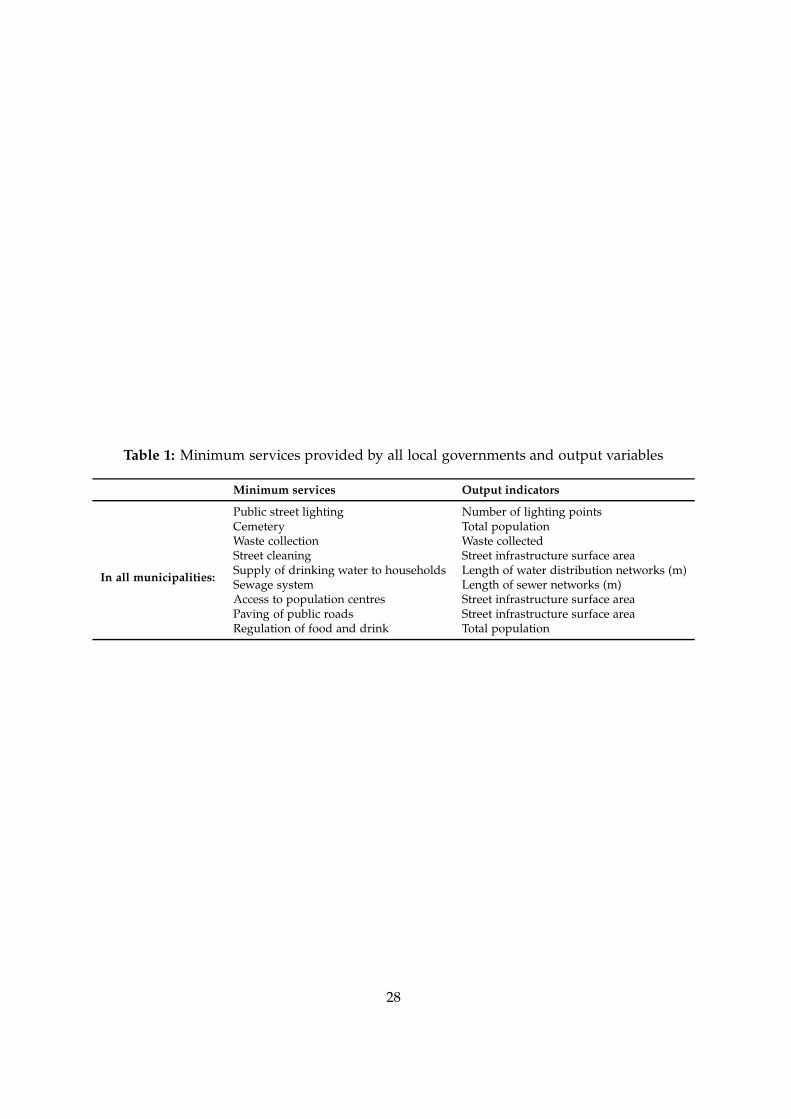
Table 1: Minimum services provided by all local governments and output variables

Minimum services Output indicators

In all municipalities:

Public street lighting Number of lighting pointsCemetery Total populationWaste collection Waste collectedStreet cleaning Street infrastructure surface areaSupply of drinking water to households Length of water distribution networks (m)Sewage system Length of sewer networks (m)Access to population centres Street infrastructure surface areaPaving of public roads Street infrastructure surface areaRegulation of food and drink Total population

28

Table 2: Descriptive statistics for data in inputs and outputs,period 2008-2013

Mean S.d.

INPUTSa

Total costs (X1) 6,856,864.55 7,990,865.20

OUTPUTSTotal population (Y1) 7,555.36 8,460.33Street infrastructure surface areab(Y2) 336,673.55 325,808.07Number of lighting points (Y3) 1,519.78 1,567.02Tons of waste collected (Y4) 4,216.73 19,720.07Length of water distribution networksb(Y5) 50,503.12 93,877.89Length of sewer networksb(Y6) 29,650.29 32,424.83

a In thousands of euros.b In square metres.

29

Table 3: Combinations of error and inefficiency terms in Monte Carlo simulations to modelscenarios

We simulate six different combinations for the error (συ) and inefficiency (σu) terms, in order to model variousreal scenarios. The rows represent the variation of the error term, while the columns represent the variation of theinefficiency term. The Λ parameter is the ratio between σu and συ, which sets each scenario.

σu = 0.01 σu = 0.05 σu = 0.1

συ = 0.01 s1: Λ = 1.0 s3: Λ = 5.0 s5: Λ = 10.0συ = 0.05 s2: Λ = 0.2 s4: Λ = 1.0 s6: Λ = 2.0

30

Table 4: Baseline results with Cobb-Douglas cost function

This table provides the baseline results for the performance of the methodologies in the Monte Carlo experiment. We simulate six scenarios, which representdifferent combinations for the error (συ) and inefficiency (σu) terms.

Biasa RMSEb Upward Biasc Kendall’s τd

DEA FDH Order-m KSW DEA FDH Order-m KSW DEA FDH Order-m KSW DEA FDH Order-m KSW

s1: συ = 0.01, σu = 0.01n=100 -0.0298 0.0074 0.0231 -0.0350 0.0330 0.0096 0.0307 0.0375 0.0500 0.9800 0.9900 0.0100 0.2491 0.1227 0.0615 0.2549n=200 -0.0348 0.0070 0.0287 -0.0391 0.0376 0.0094 0.0370 0.0415 0.0250 0.9600 0.9850 0.0050 0.2573 0.1590 0.0790 0.2588

s2: συ = 0.05, σu = 0.01n=100 -0.0892 -0.0111 0.0049 -0.1006 0.1013 0.0338 0.0399 0.1111 0.0500 0.6400 0.6900 0.0100 0.0681 0.0551 0.0511 0.0687n=200 -0.1028 -0.0205 0.0043 -0.1130 0.1134 0.0428 0.0466 0.1225 0.0250 0.5000 0.6200 0.0050 0.0707 0.0597 0.0542 0.0705

s3: συ = 0.01, σu = 0.05n=100 -0.0182 0.0322 0.0477 -0.0246 0.0238 0.0392 0.0548 0.0285 0.1200 1.0000 1.0000 0.0600 0.6753 0.4443 0.3169 0.6877n=200 -0.0239 0.0289 0.0512 -0.0293 0.0281 0.0351 0.0581 0.0325 0.0700 0.9900 1.0000 0.0350 0.6843 0.5192 0.3812 0.6911

s4: συ = 0.05, σu = 0.05n=100 -0.0707 0.0133 0.0303 -0.0832 0.0857 0.0410 0.0528 0.0960 0.0900 0.7500 0.8100 0.0400 0.3060 0.2547 0.2415 0.3059n=200 -0.0849 0.0024 0.0279 -0.0963 0.0972 0.0421 0.0565 0.1072 0.0500 0.6300 0.7550 0.0250 0.3132 0.2710 0.2564 0.3123

s5: συ = 0.01, σu = 0.1n=100 -0.0101 0.0525 0.0684 -0.0177 0.0203 0.0624 0.0768 0.0238 0.2000 1.0000 1.0000 0.1000 0.8057 0.5928 0.5146 0.8182n=200 -0.0170 0.0453 0.0689 -0.0232 0.0230 0.0537 0.0763 0.0275 0.1150 0.9950 1.0000 0.0600 0.8174 0.6586 0.5738 0.8254

s6: συ = 0.05, σu = 0.1n=100 -0.0580 0.0347 0.0519 -0.0724 0.0755 0.0591 0.0722 0.0869 0.1300 0.8200 0.8800 0.0700 0.4996 0.4170 0.4030 0.4990n=200 -0.0726 0.0207 0.0485 -0.0854 0.0867 0.0530 0.0717 0.0974 0.0750 0.7200 0.8400 0.0400 0.5065 0.4403 0.4332 0.5065

a The bias reports the difference between the estimated and true efficiency scores. When it is negative (positive), the estimators are underestimating (overestimating) the true efficiency.b The RMSE (root mean squared error) measures the standard deviation or error from the true efficiency.c The upward bias is the proportion of estimated efficiencies larger than the true efficiencies (returning a value of 1). The desired value is 0.5. The values less (greater) than 0.5 indicate underestimation(overestimation) of cost efficiencies.d Kendall’s τ shows the correlation coefficient for the efficiency ranks between true and estimated efficiency scores.

31

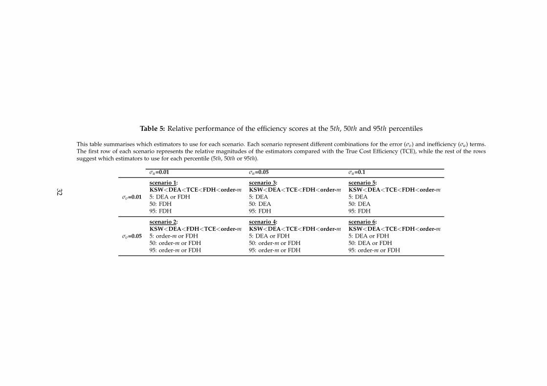
Table 5: Relative performance of the efficiency scores at the 5th, 50th and 95th percentiles

This table summarises which estimators to use for each scenario. Each scenario represent different combinations for the error (συ) and inefficiency (σu) terms.The first row of each scenario represents the relative magnitudes of the estimators compared with the True Cost Efficiency (TCE), while the rest of the rowssuggest which estimators to use for each percentile (5th, 50th or 95th).

σu=0.01 σu=0.05 σu=0.1

συ=0.01

scenario 1: scenario 3: scenario 5:KSW<DEA<TCE<FDH<order-m KSW<DEA<TCE<FDH<order-m KSW<DEA<TCE<FDH<order-m5: DEA or FDH 5: DEA 5: DEA50: FDH 50: DEA 50: DEA95: FDH 95: FDH 95: FDH

συ=0.05

scenario 2: scenario 4: scenario 6:KSW<DEA<FDH<TCE<order-m KSW<DEA<TCE<FDH<order-m KSW<DEA<TCE<FDH<order-m5: order-m or FDH 5: DEA or FDH 5: DEA or FDH50: order-m or FDH 50: order-m or FDH 50: DEA or FDH95: order-m or FDH 95: order-m or FDH 95: order-m or FDH

32

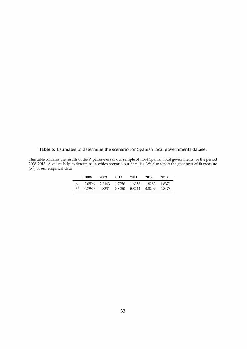
Table 6: Estimates to determine the scenario for Spanish local governments dataset

This table contains the results of the Λ parameters of our sample of 1,574 Spanish local governments for the period2008–2013. Λ values help to determine in which scenario our data lies. We also report the goodness-of-fit measure(R2) of our empirical data.

2008 2009 2010 2011 2012 2013

Λ 2.0596 2.2143 1.7256 1.6953 1.8283 1.8371R2 0.7980 0.8331 0.8250 0.8244 0.8209 0.8478

33

Table 7: Summary statistics for efficiency results in Spanish local governments

DEAMean Median Min Max Q1 Q3

2008 0.4943 0.4689 0.0437 1.0000 0.3611 0.60382009 0.5843 0.5740 0.1257 1.0000 0.4633 0.68302010 0.5212 0.4953 0.1312 1.0000 0.4017 0.61352011 0.5314 0.5092 0.1359 1.0000 0.4104 0.62372012 0.5316 0.5128 0.1079 1.0000 0.4077 0.64292013 0.5712 0.5591 0.1138 1.0000 0.4458 0.6823

2008–2013 0.5390 0.5199 0.1097 1.0000 0.1761 0.6415

FDHMean Median Min Max Q1 Q3

2008 0.7444 0.7678 0.0808 1.0000 0.5644 1.00002009 0.8186 0.8563 0.2045 1.0000 0.6821 1.00002010 0.7761 0.7848 0.1559 1.0000 0.6251 1.00002011 0.7453 0.7434 0.2037 1.0000 0.5808 0.98922012 0.7630 0.7737 0.1497 1.0000 0.6104 1.00002013 0.7619 0.7721 0.1497 1.0000 0.6104 0.9999

2008–2013 0.7682 0.7830 0.1574 1.0000 0.2053 0.9982

Order-mMean Median Min Max Q1 Q3

2008 0.8089 0.8255 0.0834 1.9813 0.6312 1.00002009 0.8691 0.8926 0.2122 1.7369 0.7318 1.00132010 0.8385 0.8515 0.2172 1.8080 0.6938 1.00002011 0.8088 0.8100 0.2368 2.0281 0.6497 1.00002012 0.8222 0.8358 0.1797 1.8914 0.6644 1.00002013 0.8209 0.8328 0.1785 1.9204 0.6609 1.0000

2008–2013 0.8281 0.8414 0.1846 1.8944 0.6720 1.0002

KSWMean Median Min Max Q1 Q3

2008 0.4421 0.4239 0.0400 1.0000 0.3183 0.54542009 0.5384 0.5297 0.1179 1.0000 0.4250 0.63702010 0.4541 0.4294 0.0563 1.0000 0.3420 0.53992011 0.4752 0.4558 0.1178 1.0000 0.3697 0.55582012 0.4677 0.4477 0.0134 1.0000 0.3503 0.56872013 0.4846 0.4711 0.0118 1.0000 0.3678 0.5848

2008–2013 0.4770 0.4596 0.0595 1.0000 0.3622 0.5719

34

Table 8: Rank correlation Kendall coefficients between the average cost efficiency estimates ofthe four methodologies for the period 2008–2013

DEA FDH Order-m KSW

DEA 1.0000 0.6687 0.6463 0.9004FDH 0.6687 1.0000 0.7755 0.6136Order-m 0.6463 0.7755 1.0000 0.5801KSW 0.9004 0.6136 0.5801 1.0000

35

Figure 1: Violin plots in scenario 1 and 2 for 5th, 50th and 95th percentiles of cost efficiencyestimates under a Cobb-Douglas cost function.

TCE DEA FDH Order-m KSW

0.9

0.90

0.95

1.00

1.05

1.10

(a) S1, 5th percentile, n=100

TCE DEA FDH Order-m KSW

0.8

0.9

1.0

1.10

(b) S2, 5th percentile, n=100

TCE DEA FDH Order-m KSW0.90

0.95

1.00

1.05

1.10

(c) S1, 50th percentile, n=100

TCE DEA FDH Order-m KSW

0.8

0.9

1.0

1.10

(d) S2, 50th percentile, n=100

TCE DEA FDH Order-m KSW

0.95

1.00

1.05

1.10

(e) S1, 95th percentile, n=100

TCE DEA FDH Order-m KSW

0.8

0.9

1.0

1.10

1.20

(f) S2, 95th percentile, n=100

36

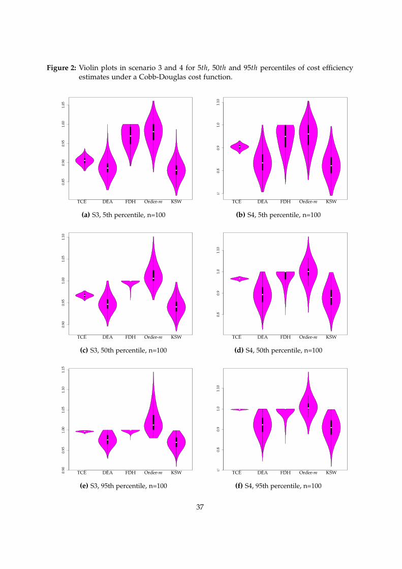
Figure 2: Violin plots in scenario 3 and 4 for 5th, 50th and 95th percentiles of cost efficiencyestimates under a Cobb-Douglas cost function.

TCE DEA FDH Order-m KSW

0.9

0.85

0.90

0.95

1.00

1.05

(a) S3, 5th percentile, n=1000.7

TCE DEA FDH Order-m KSW

0.8

0.9

1.0

1.10

(b) S4, 5th percentile, n=100

TCE DEA FDH Order-m KSW

0.90

0.95

1.00

1.05

1.10

(c) S3, 50th percentile, n=100

TCE DEA FDH Order-m KSW

0.8

0.9

1.0

1.10

(d) S4, 50th percentile, n=100

TCE DEA FDH Order-m KSW0.90

0.95

1.00

1.05

1.10

1.15

(e) S3, 95th percentile, n=100

0.7 TCE DEA FDH Order-m KSW

0.8

0.9

1.0

1.10

(f) S4, 95th percentile, n=100

37

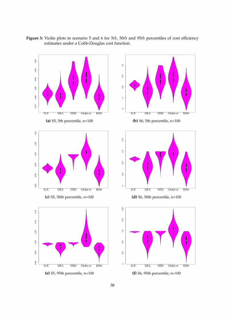
Figure 3: Violin plots in scenario 5 and 6 for 5th, 50th and 95th percentiles of cost efficiencyestimates under a Cobb-Douglas cost function.

TCE DEA FDH Order-m KSW

0.9

0.75

0.80

0.85

0.90

0.95

1.00

(a) S5, 5th percentile, n=1000.6

0.7

TCE DEA FDH Order-m KSW

0.8

0.9

1.0

(b) S6, 5th percentile, n=100

TCE DEA FDH Order-m KSW

0.85

0.90

0.95

1.00

1.05

1.10

(c) S5, 50th percentile, n=100

0.7

TCE DEA FDH Order-m KSW

0.8

0.9

1.0

1.10

(d) S6, 50th percentile, n=100

TCE DEA FDH Order-m KSW

0.90

0.95

1.00

1.05

1.10

1.15

(e) S5, 95th percentile, n=100

0.7

TCE DEA FDH Order-m KSW

0.8

0.9

1.0

1.10

1.20

(f) S6, 95th percentile, n=100

38

Figure 4: Violin plots of cost efficiency estimates in Spanish local governments

0.5

1.0

1.5

DEA FDH Order−m KSW

Den

sity

of e

ffici

ency

sco

res

Figure 5: 2008–2013

39