39PB

Government Expenditure, Agricultural Productivity, and Poverty Reduction in Indonesia:

A Simultaneous Equations Approach

Puji Eddi Nugroho*

インドネシアにおける政府支出、農業生産性、および貧困削減̶ 同時方程式アプローチ ̶

プジ　エディ　ヌグロホ*

Abstract

This paper aims to empirically analyze the direct and indirect effects of various

governmental development expenditures to enhance agricultural productivity and combat

poverty by means of increasing wage levels, stabilizing prices, and boosting non-agricultural

employment. A simultaneous equation approach is formulated not only to rank different

types of spending in terms of their effects on productivity and poverty, but also to calculate

the number of poor people reduced for an additional unit of spending. This study uses

provincial level panel data from 2005 to 2014 and employs the three-stage least squares

(3SLS) method to estimate the equation system.

The result indicates that to increase agricultural productivity and to reduce poverty, the

Government of Indonesia should give highest priority to additional spending in agriculture

and education. Agricultural and education expenditures not only appear statistically

significant to boost mostly productivity levels, but also show the highest poverty reduction

impact per additional Rupiah spent. Moreover, spending on roads, irrigation, and power

are seen to have a limited effect on agricultural growth and little marginal return on

poverty reduction. Generally, the various expenditures for each of these two goals could be

interpreted as complementary. This suggests that there are limited trade-offs between their

effects on agricultural productivity and poverty reduction. The result also shows that the

poverty can be alleviated through improving agricultural productivity and creating non-farm

employment.

＊PhD Program, Graduate School of Asia-Pacific Studies, Waseda University Email: eddi_nugroho@fuji.waseda.jp

Graduate School of Asia-Pacific Studies, Waseda UniversityJournal of the Graduate School of Asia-Pacific StudiesNo.34 (2017.9) pp.39-54

4140

1. Introduction

The relationship between poverty and government expenditure has been given much attention

by the government and researchers. Some researchers believe that increasing public spending

can reduce the poverty rate through enhanced economic growth. Poverty is one of the problematic

issues in the world particularly in Indonesia. Currently, more than 28 million people or 10.9 percent

of the total Indonesian population are still poor, living below the poverty line. Strong economic

growth in Indonesia has helped in reducing poverty, coming down to 11.1％ in 2015, compared to

15.97％ in 2005. But the pace of reduction is slowing down. The poverty reduction of 0.27％ points

over the last two years is the smallest declining over the last decade. Based on the World Bank data,

the Indonesia poverty reduction from 2012 to 2014 with national poverty line is 0.6％ points, lowest

be compared by 1.1％ points in Malaysia, 2.1％ points in Thailand, and 3.7％ points in Vietnam. In

addition, Indonesia poverty reduction from 2012 to 2013 is 1.9％ points, one fourth of China that

achieves 4.6％ points with poverty headcount ratio at $1.90 a day.

One of the key contributing components to economic growth is governmental expenditures.

The government expenditures that have been spent will create the investments as their outcomes.

During the period 2005-2014, the Government of Indonesia has applied an expansionary fiscal policy.

This policy is said to have a positive effect on output at both the national and regional level, and is

expected to accelerate economic growth (pro growth), to create the jobs (pro-job), and to eradicate

poverty (pro-poor). Therefore, the government needs to determine the public spending allocation

and prioritize programs that most effectively contribute to poverty alleviation and economic growth.

This study intends to empirically analyze the effects of six types of government development

expenditure namely, agriculture, irrigation, roads, education, health, and power on agricultural

productivity and poverty reduction in Indonesia. Also, the number of poor people lifted above

the poverty line for additional units of such spending is calculated. This study tries to answer the

following research questions: Do the various types of government development expenditure have an

effect on agricultural productivity and poverty rate? If so, to what degree? For government institutions

and policymakers, the findings of this study will provide insights on which type of government

expenditures have the largest impact on agricultural productivity and poverty reduction.

The rest of this study is organized as follows. Section 2 briefly reviews the relevant literature.

The framework, model specifications, and data are discussed in section 3. Section 4 presents and

discusses the empirical results. Lastly, section 5 concludes.

2. Literature Review

Literature has examined the effect of government spending on poverty in some developing

countries. Fan and Rao (2008) countries finds that agricultural spending, irrigation, education, and

roads all contributed strongly to poverty alleviation in rural areas. Fan et al. (2000, 2004, and 2008)

examine the relationship between government expenditure and economic growth and poverty

alleviation in rural areas in India, Vietnam and Uganda. Their results indicate that government

4140

expenditure has a significant and positive effect on economic growth and a negative effect on

poverty incidence. Building rural roads, conducting agricultural research and extension have the

largest impact on poverty reduction in the three countries. The growth in agriculture contributes

to poverty reduction in rural areas indirectly through increased rural wages and farm and nonfarm

employment. Moreover, agricultural growth can contribute to poverty reduction in urban areas by

lowering food prices for urban residents and contributing to national economic growth. In India

study obviously shows that additional government expenditure on roads has the largest poverty

reduction impact, as well as a significant impact on productivity growth.

Moreover, Fan et al. (2004) by using provincial level data for 1953-2000 in China, find that

government spending on production-enhancing investments, such as agricultural R&D and

irrigation, rural education, and infrastructure (including roads, electricity, and telecommunications),

all contributed to agricultural productivity growth and reduced rural poverty. Government

expenditure on education had the largest impact on poverty reduction and very high returns to

growth in agriculture and the non-farm sector. Furthermore, Fan et al. (2004) by using data from

1977 to 1999 in Thailand, finds that public investments in agriculture, irrigation, education, roads,

and electricity, still have positive marginal impacts on agricultural productivity growth and poverty

reduction. The largest impact to poverty reduction is electricity sector then followed by agriculture,

roads, education and irrigation sector respectively.

In terms of composition in government expenditure, Gupta et al. (2005) analyzes the effect of

fiscal consolidation and expenditure composition on economic growth in 39 low income countries in

the period 1990-2000. They conclude that development expenditures affect positively on economic

growth and current expenditure affect negatively on economic growth. Hasan and Quibria (2004)

find that while growth in agriculture is most effective for poverty reduction in Sub-Saharan Africa

and South Asia, growth in industry is most effective for East Asia and in services for Latin America.

Ravallion and Datt (1996) and Foster and Rosenwzweig (2004) for India, and Suryahadi and Sumarto

(2009) for Indonesia, all find that agricultural growth is key for reducing poverty in rural areas.

The other Indonesia empirical study with single equation such as Lanjouw et al. (2001) found

that spending on primary education tends to be pro-poor, while spending on higher education is

less beneficial to the poor. In addition, Indriawan and Muhyiddin (2007) found that government

spending has positive correlation to per capita income growth, but statistically not significant.

However, there are still limited numbers of studies on the government spending and its impact to

agriculture productivity and poverty reduction in Indonesia with simultaneous equation model at

current period. Moreover, the most studies from Fan et.al. are empirical studies in rural area using

data period earlier than 2000. Currently, poverty is not only in rural area but also in urban area.

Therefore, this paper addresses this lacuna in the literature for the case of Indonesia.

4342

3. Methodology

3.1 Framework and Model

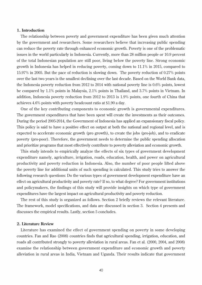
Government investments are the outputs or outcomes of government spending. Government

expenditures and their investments affect poverty reduction through different channels. They not

only contributed to agricultural productivity growth and indirectly to poverty reduction, but they

have created nonagricultural jobs, increased wages, changed prices as described in Figure 1.

The author adapts the structural equations system that was introduced and developed by

Shenggen Fan, et al. (2000) at the International Food Policy Research Institute (IFPRI). This model

consists of many simultaneous equations to estimate the direct and indirect effect of various sectors

of government expenditures on agricultural productivity and poverty. It is difficult to depict and

to rank these different effects using a single equation approach. Moreover, the model allows for

calculation of economic return measured by the number of poor people raised above the poverty

line for additional units of spending on different sectors.

This approach also allows us to explore the interaction among various variables of interest

simultaneously. The specification of simultaneous equations model violates the ordinary least

square (OLS) assumption of zero covariance between the disturbance term and the independent

variables. Therefore, estimation results obtained by OLS will be biased and inconsistent. Such

simultaneous equations bias can be corrected by applying various instruments that is correlated

with the endogenous variable while uncorrelated with the disturbance term.

However, the disturbance from these terms of these equations are likely to be contemporaneously

correlated because unconsidered factors that influence the disturbance term in one equation

probably also influence the disturbance term in other equations. Ignoring this contemporaneous

correlation and estimating these equations separately leads to inefficient estimates of the

　　 Source: Created by author based on Fan et. al (2000)

Fig 1: The Framework

4342

coefficients. This paper applies a 3SLS method to estimate all equations simultaneously to obtain

more efficient results. Under standard condition of normally distributed disturbances, 3SLS method

is asymptotically efficient (Greene, 2002).

Moreover, this paper employs fixed effect model to eliminate most of bias due to provincial

invariant fixed effects with province dummy variables. Double-log functional forms are used for all

the equations in system. In addition, all of variables are taken from provincial level and and each

variable is also observed at provincial level. Thus, this study uses province as unit of analysis.

Equation (1) to (10) presents the formal structure of the equation system. Poverty equation

(1) is modeled as a function of agricultural productivity (AP), wages (WAGE), nonagricultural

employment (NAEMPLYP), and terms of trade (TT), one year lag of the number of population

(POP-1), and one year lag of Regional Gross Domestic Product per capita (RGDP-1).1

(1) P = f ( AP, WAGE, NAEMPLY, TT, POP-1, RGDP-1 )

Agricultural productivity variable is included because agricultural still accounts for important

share of total income of households. This study uses agricultural labor productivity as a proxy

for agricultural performance. Income from nonagricultural employment is significant resource

for residents. Wage rate and nonagricultural employment are also important sources of income

in Indonesia. Wage variable is included in order to distinguish the impacts of wage and non-farm

workers on poverty. TT measures the effect of the ratio agricultural prices to nonagricultural

prices on poverty rate. The first four variables above had a significant effect on the poverty based

on previous study in India. Population as the employment resources also contributes to poverty

reduction. The RGDP per capita variable is included to control for the remaining income effect

besides AP, Wages, and NAEMPLYP variable on poverty reduction.

(2) AP = f ( AGDE, AGDE-1, …. AGDE-i, IR, ROADS, PVELE,

YSCHO, HEALC, RGDP-1, RAIN )

Agricultural productivity is modeled as a function of government spending in agriculture (AGDE),

government investment on irrigation (IR), roads (ROADS), electricity (PVELE), education (YSCHO),

health (HEALC), one year lagged RGDP per capita, and rainfall (RAIN) as equation 2. Investment

variables depict the effect of technologies, infrastructures, education on productivity. The lagged

GDP variable controls the effect of economic performance on productivity and the rainfall variable

captures the weather effects.

(3) WAGE = f (AP, ROADS, PVELE, YSCHO, HEALC, RGDP-1 , INF)

Equation (3) is a wages determination function. Wages rate is determined by agricultural

productivity (AP); government investments in roads (ROADS), electricity (PVELE), education

(YSCHO), and health (HEALC); one year lagged RGDP; and inflation (INF). Regional minimum

wage in this estimation is used as proxy of labor wage variable. Then, inflation variable is included

1 One year lag for population and GDP variables used to avoid the endogeneity problem of these variables in the poverty equation (Fan et. al. 2000).

4544

in this equation to represent the effect of goods and services prices on cost of living as determinant

for government to decide the minimum wage.

(4) NAEMPLYP = f (AP, ROADS, PVELE, YSCHO, HEALC, RGDP-1)

Equation (4) determines percentage of nonagricultural employment. NAEMPLY is modeled a

function of agricultural productivity (AP), improvement government investments in roads (ROADS),

electricity (PVELE), education (YSCHO), and health (HEALC), and one year lagged RGDP.

Investment variables also portray the effect of infrastructures, technologies, education on non-farm

employment.

(5) TT = f ( AP, APN)

Equation (5) models the relationships between the term of trade and the agricultural productivity

growth at both province level (AP) and national level (APN). It shows how increased agriculture

productivity at province and national level influence the agriculture prices.

(6) IR = f ( IRE, IRE-1,…, IRE-j)

(7) ROADS = f ( ROADE, ROADE-1, …, ROADE-k )

(8) YSCHO = f ( EDE, EDE-1, …, EDE-l)

(9) PVELE = f ( PWRE, PWRE-1,..., PWRE-m)

(10) HEALC = f ( HEALE, HEALE-1,..., HEALE-n)

Equations (6) to (10) are the functions of irrigation, roads, education, electricity, and health that

were determined by current and some lags of past government spending on each sector (distributed

lagged estimation). These models to capture the long lead times involved in transforming actual

government spending into capital stock of investment. Thus, spending variables in this study

are exogenous variables. Based on the previous study in India and China, government spending

variables in total each of estimation had a significant effect on their investments stock.

3.3. Data and Variables

The main data set in the econometric analysis comes from the Ministry of Finance of Indonesia,

the World Bank, and Statistical Yearbook of Indonesia published by Statistics Indonesia period 2005-

2014 as defined and described in Table 1, Table 2, and Table 3. Considering the availability of data

from new provinces and the Indonesia budget classification reform since 2005, this study uses panel

data that covers period 2005-2014 and encompasses information on up to 33 provinces.

Government development expenditures data based on sector decomposition per province was

obtained from Ministry of Finance of Republic Indonesia and the World Bank. These expenditures

are realization of development spending aggregate from central government and local governments

(33 provinces and 497 districts) into province level in real values after deflated by provincial GDP

deflator (2000 as the base year).

4544

Table 1: Definition of Exogenous and Endogenous Variables

Variables Definition Unit SourceExogenous variablePOP The number of population. people WBRGDP Regional Gross Domestic Product per capita in real price. million rupiah WBAPN Agricultural Labor Productivity (AP) at national level. million

rupiah/peopleWB

RAIN Annual rainfall or number of precipitation. mm SIINF Inflation rate is represented by the GDP deflator. indexIRE The sum of development expenditure realization of both central and local

government on irrigation including irrigation special allocation fund in constant price.

million rupiah MoF

AGDE The sum of development expenditure realization of both central and local government on agriculture that covers spending in food security, forestry, marine and fisheries including agricultural special allocation fund, fund for high yield varieties, machinery of farmer and fisherman, and fertilizer in constant price.

million rupiah MoF

ROADE The sum of development expenditure realization of both central and local government on roads including roads special allocation fund in constant price.

million rupiah MoF

EDE The sum of development expenditure realization of both central and local government on education including spending for religion, library, youth, sports, school operational grant for elementary school, and scholarships in constant price.

million rupiah MoF

PWRE Development expenditure realization on power from central government that covers rural electric development and power development program in constant price.

million rupiah MoF

HEALE The sum of development expenditure realization of both central and local government on health including spending on family planning program in constant price.

million rupiah MoF

Endogenous variableP Poverty headcount ratio, measured by percentage of population living below

national poverty line. percent SI

WAGE Labor wage in agricultural and non-agricultural sectors is represented by the real regional minimum wage per month.

rupiah SI

NAEMPLYP Percentage of nonagricultural employment in total employment. WBAP Agricultural productivity per labor measured by agricultural RGDP divided by

the number of employee in agriculture including independent farmers. million

rupiah/peopleWB

TT Terms of trade measured by the ratio of agricultural prices (agricultural GDP deflator) to nonagricultural prices (non-agricultural GDP deflator).

index WB

YSCHO Mean years of schooling of adults (aged 15 or over). year SIROADS Road density, length of roads in asphalt, dirt, gravel, and others (National,

Province, and District roads) per 1,000 km2 area; accumulated capital stock.km/1000 km2

area WB

IR Percentage of wetland area that is irrigated (accumulated capital stock) percent WBPVELE Percentage of household that has access to electricity (accumulated capital

stock).percent WB

HEALC The number of Public Health Center per 100,000 people (accumulated capital stock).

unit/100,000 people

WB

Notes: ‐ Exogenous variables whose values are determined outside the model, whereas endogenous variables are determined

within the model.‐All variables in level at estimations were first transform in log form.Source: Author’s compilation data from Statistics Indonesia (SI), World Bank (WB), and Ministry of Finance Republic of

Indonesia (MoF).

4746

Table 2: Descriptive Statistics

Variable Obs. Mean Std. Dev. Minimum Maximum

Poverty Incidence (P) 328 14.91201 8.131599 3.48 41.52Agricultural Productivity (AP) 262 8.531558 3.895795 2.644412 20.86405National Agric. Product. (APN) 262 8.531558 0.6987339 7.607958 9.772927Wage Rate (WAGE) 325 399527.3 105753.6 215651.3 874143.2Non-Agric. Employment (NAEMPLYP) 295 54.38357 16.62604 21.95743 99.66521Terms of Trade (TT) 264 0.9705094 0.1418106 0.5221729 1.374203Population (POP) 330 7168620 1.01E＋07 689446.2 4.60E＋07Regional GDP (RGDP) 329 8.858697 7.802079 1.976154 47.37181Rainfall (RAIN) 266 2196.509 1036.046 1.5 5228Inflation (INF) 330 2.289545 0.6279954 1.15 5.37Irrigation Rate (IR) 297 62.63697 25.9199 6.354955 100Roads Density (ROADS) 323 716.8859 1675.864 27.46065 10683.57Years of Schooling (YSCHO) 264 7.808258 0.873903 5.06 10.36Electricity Rate (PVELE) 294 85.54712 14.11791 38.19 99.97Public Health Center (HEALC) 297 5.662015 2.827178 1.824541 17.26428Agricultural Spending (AGDE) 330 360215.6 379510.7 27350.99 2882594Irrigation Spending (IRE) 326 82806.09 90952.19 755.18 625971.5Roads Spending (ROADE) 330 309183.8 255584.3 17073.5 1485550Education Spending (EDE) 330 2479583 3251339 137240.1 2.36E＋07Power Spending (PWRE) 329 223672.4 222134.2 7787 1300000Health Spending (HEALE) 330 674930.1 992237.3 30322.93 6494138

Note: All variables in standard form (not in log form) Source: Author’s calculation.

Table 3: Matrix Correlation Table

Variables （1）（2）（3）（4）（5）（6）（7）（8）（9）（10）（11）（12）（13）（14）（15）（16）（17）（18）（19）（20）（21）（1）1nP 1.00

（2）1nAP -0.59 1.00

（3）1nAPN -0.22 0.25 1.00

（4）1nWAGE -0.37 0.29 0.25 1.00

（5）1nNAEMPLYP -0.64 0.61 0.23 0.19 1.00

（6）1nTT -0.20 0.07 0.03 0.15 0.22 1.00

（7）1nPOP-1 -0.14 0.09 0.03 -0.29 0.35 0.10 1.00

（8）1nGDP-1 -0.56 0.78 0.17 0.28 0.52 -0.02 0.26 1.00

（9）1nRAIN -0.18 0.14 0.34 0.15 0.04 -0.07 -0.06 0.13 1.00

（10）1nINF 0.02 0.24 0.69 -0.17 0.02 -0.27 0.05 0.29 0.28 1.00

（11）1nIR 0.23 -0.24 -0.13 0.05 0.15 0.06 -0.03 -0.29 -0.14 -0.26 1.00

（12）1nROADS -0.41 0.21 0.11 0.06 0.68 0.36 0.48 0.22 -0.08 -0.07 0.35 1.00

（13）1nYSCHO -0.49 0.54 0.21 0.38 0.61 0.49 0.12 0.42 0.05 -0.05 0.05 0.49 1.00

（14）1nPVELE -0.57 0.58 0.21 0.08 0.81 0.29 0.38 0.37 0.14 0.01 -0.03 0.56 0.67 1.00

（15）1nHEALC 0.37 -0.20 0.10 0.28 -0.56 -0.14 -0.74 -0.25 0.16 0.12 0.02 -0.56 -0.17 -0.53 1.00

（16）1nAGDE -0.25 0.15 0.22 0.13 0.28 0.23 0.67 0.39 0.01 0.09 -0.02 0.45 0.31 0.25 -0.26 1.00

（17）1nIRE 0.05 -0.23 -0.32 -0.11 0.02 0.11 0.50 -0.08 -0.08 -0.29 0.28 0.30 0.02 0.05 -0.21 0.49 1.00

（18）1nROADE -0.05 0.00 0.49 0.25 0.04 0.07 0.42 0.18 0.08 0.29 0.05 0.20 0.09 0.00 0.05 0.69 0.31 1.00

（19）1nEDE -0.03 0.19 0.21 0.01 0.47 0.24 0.88 0.38 0.04 0.08 0.03 0.61 0.36 0.46 -0.57 0.87 0.52 0.59 1.00

（20）1nPWRE -0.17 0.18 0.55 0.19 0.15 0.02 0.46 0.35 0.21 0.37 -0.12 0.23 0.17 0.14 -0.04 0.72 0.22 0.79 0.61 1.00

（21）1nHEALE -0.33 0.20 0.15 0.10 0.43 0.17 0.77 0.49 0.06 0.07 0.03 0.55 0.31 0.35 -0.44 0.92 0.51 0.59 0.94 0.62 1.00

Note: All variables in log form.Source: Author’s calculation.

4746

3.2. Test of Investment Lags

This paper uses statistical tools to test and to determine the appropriate length of lag for each

spending in investment equations. Author used Akaike’s Information Criterion (AIC) and chose the

lag length that minimized the value of AIC. This procedure led to lags of five years for agriculture,

nine years for roads, five years for education, two years for irrigation, two years for electricity, and

six years for health. These lags are similar compared to lags obtained for India study and quite short

compared to much longer lags obtained the United States.

4. Empirical Result and Analysis

This research uses 3SLS method to estimate the equation system. The estimation results are

presented in Table 4. The estimated poverty equation (equation (1)) confirms that an improvement

in agricultural productivity, percentage of non-agricultural employment, and population have

contributed significantly to reducing poverty. It shows that the impact of income on poverty was

captured by agricultural productivity. Study in India by Fan et al. (2000) finds that the increasing

of population does not contribute to poverty reduction meanwhile, in Indonesia it contributes

significantly to poverty reduction. However, increasing minimum wage has positive but insignificant

correlation to poverty. The government resources should be targeted to improve non-agriculture

employment rather than to improve minimum wage. It is consistent with finding by Bird, Kelly

and Chris Manning (2008) in which minimum wage policy is unlikely to be an effective antipoverty

instrument in Indonesia. The coefficient of the terms of trade variable is negative but statistically

insignificant to poverty. Otherwise, the terms of trade, and regional GDP variables are negatively

but insignificantly correlated to poverty.

The estimate for equation agricultural labor productivity (equation (2)) shows that increases

in total spending on agriculture and means years of schooling have contributed significantly to

agricultural productivity. The coefficient for agricultural spending in this study is the sum of current

and the past five year coefficients. This result supports the study in India by Ravallion and Datt

(1996) and Foster and Rosenwzweig (2004), and a study in Indonesia by Suryahadi and Sumarto

(2009). This improved agricultural spending includes allocation for providing the high yield varieties,

machinery of farmer and fisherman, and fertilizer as the implementation of agricultural technologies.

Improved mean years of schooling could upgrade and improve the knowledge of farmers in

agriculture activities. It induces agricultural growth by raising productivity. Rainfall and investments

on irrigation, roads, and electricity are all positively insignificant to agricultural productivity.

Otherwise, the increasing of health center ratio has negative correlation to agricultural productivity.

It is because most of agricultural employees that living in remote rural area have difficulties to access

health centers. Therefore, health status of agricultural labors is poor as a result their productivities

are reducing. It indicates that health center facilities are more beneficial for urban people which

mostly as non-agricultural employments. This phenomenon supports a study result in Indonesia

4948

is that public health center facilities are distributed with a slight pro-poor (Lanjouw et. al. 2007,

p.33). Moreover, there is a trend that healthier persons are likely either working or moving on non-

agricultural employment. This is in line with result of equation (4) is that increased health investment

contributes significantly to percentage of non-agricultural employment. This is one of evidences that

Table 4: Three-Stage Least Squares (3SLS) Estimation Results

Dependent Variable

Poverty Incidence

Agric.productivity

WageRate

Non-Agric.Employment

Termsof Trade

IrrigationRate

RoadsDensity

Years ofSchooling

ElectricityRate

Public HealthCenter

（1） （2） （3） （4） （5） （6） （7） （8） （9） （10）AgricultureProductivity

-3.59(0.063)

＊＊＊ -0.043(0.063)

0.169(0.054)

＊＊＊ 0.039(0.067)

Wage Rate0.114

(0.119)Non-AgricultureEmployment

-0.322(0.126)

＊＊＊

Terms of Trade-0.125

(0.112)

Population-1-1.107

(0.228)

＊＊＊

AgriculturalSpending

0.254(0.094)

＊＊＊

Irrigation Rate0.002

(0.027)

Roads Density0.067

(0.248)-0.193

(0.134)0.090

(0.107)

Years Schooling1.762

(0.825)

＊＊ 1.220(0.490)

＊＊ 0.636(0.389)

Electricity Rate0.196

(0.280)-0.254

(0.153)

＊ -0.267(0.133)

＊＊

Health Center-0.763

(0.231)

＊＊＊ 0.086(0.139)

0.600(0.122)

＊＊＊

RGDP-1-0.115

(0.136)0.085

(0.222)0.657

(0.119)

＊＊＊ 0.233(0.104)

＊＊

Rainfall0.027

(0.033)

Inflation-0.189

(0.085)

＊＊

National Agric.Productivity

0.019(0.091)

Irrigation Spend.0.431

(0.137)

＊＊

Roads Spending0.075

(0.019)

＊＊＊

Educ. Spending0.101

(0.007)

＊＊＊

Power Spending0.032

(0.009)

＊＊＊

Health Spending0.094

(0.034)

＊＊＊

Constant20.840

(3.268)

＊＊＊ -4.956(1.584)

＊＊＊ 11.587(1.122)

＊＊＊ -0.087(0.140)

-0.087(0.140)

-0.746(1.584)

4.980(0.232)

＊＊＊ 0.753(0.099)

＊＊＊ 4.164(0.109)

＊＊＊ 0.748(0.447)

＊

R-square 0.996 0.984 0.980 0.990 0.941 0.868 0.999 0.996 0.982 0.996 RMSE 0.035 0.052 0.031 0.028 0.037 0.261 0.025 0.008 0.026 0.029 P 0.000 0.000 0.000 0.000 0.000 0.000 0.000 0.000 0.000 0.000 Observations 102 102 102 102 102 102 102 102 102 102

Notes: ‐ The estimations use the province dummies, but are not reported; ＊), ＊＊), and ＊＊＊) indicate significant at 10％ , 5％ , and 1％

respectively; Standard error in parenthesis; All variables in log form. ‐ Coefficients of spending are sums of coefficient of current and lagged expenditures, five years for agriculture, nine years

for roads, five years for education, two years for irrigation, two years for electricity, and six years for health. ‐ Author uses the linear combination to compute estimated coefficients, associated standard errors, and p-values

expenditures with STATA application (Greene, 1993, p.187 and Cameron and Trivedi, 2009, p.332 and 396-397). Source: Author’s estimation.

4948

Indonesia experiences the structural transformation to non-agriculture sector (Dartanto, 2013, p.10).

The estimated coefficients for wage rate equation (3) conclude that increasing in mean years of

schooling and RGDP have significantly contributed to increasing of the wage rate. Regional minimum

wage rate becomes proxy of wage rate variable in this estimation.2 Otherwise, the inflation rate and

electricity investment have negative correlation to minimum wage rate. Improving on electricity rate

could facilitate people make small business and help daily activities as a result, reduces the standard

of living cost. Then, the government keeps the real minimum wage in relatively stable although the

increased goods and service prices are occur in order to prevent a higher inflation. Moreover, roads

and health investment do not statistically significant contribute to minimum wage.

The estimated equation (4) confirms that non-agricultural employment is increased significantly

with improved agricultural productivity, RGDP, and investment in health.3 Improved agricultural

productivity and GDP growth could promote the nonagricultural sector growth that creates the

nonfarm employment opportunities. It confirms the fact that mostly, the Indonesia industries are

agricultural based industries that operationally depend on agricultural activity and as raw material

suppliers. Therefore, improved agricultural productivity will promote nonagricultural industry and as

a result, the nonagricultural employment will have increased as well. Different to study in India, is that

non-agricultural employment does not increases with agricultural productivity. Investment in health

could reduce illness and improve health status as a result the workers participate in nonagricultural

employment sector. Meanwhile, electricity rate variable has negative impact on percentage of non-

agricultural employment because the improved electricity access mainly in rural area may stimulate

the people in urban goes back to their habitation in order to working in agriculture sector which is

ever abandoned. Finally it promotes the percentage of agricultural employment.

The estimated coefficients for term trade equation (5) depict that the agricultural productivity

in region and national level all have not significantly contributed to agricultural prices. In fact,

the Government of Indonesia always wants to stabilize the agricultural prices in both harvest and

non-harvest season in order to protect both consumer and producer. The role of the government

enterprise through the Logistics Agency (BULOG) to maintain the 11 staple foods price including

agricultural products price with buying the excess supplies in the harvest period for the buffer

stock such as rice, corn, soybean, sugar, cow meat, fish, salt, chili, chicken, red onion, and garlic.

Meanwhile, in non-harvest season, the government sells the stock through the market operation

with lower price.

The estimated model shows that in one hand, improvements in agricultural productivity do

not only reduce poverty directly by increasing income (equation 1), but they also reduce poverty

2 Regional minimum wage rate is the lowest remuneration per month for workers based on the decent living cost of each province which was aggregated from district level data. Local government sets this minimum wage rate every year after conducted the monthly survey of cost of living and discussed with representative of employer and labor union (tripartite).

3 Employment is defined as all persons who worked for pay or assisted others in obtaining pay or profit for the duration at least one hour during the survey week (Indonesian Statistics).

5150

indirectly by improving the number of non-agricultural growth (equation 3). On the other hand,

they contribute to reducing poverty by increasing agricultural good prices (equation 5), although

this effect is statistically insignificant.

The estimated results for equation (6) to (10) show that government expenditures on irrigation,

roads, education, power, and health have all contributed to the stock of each capital investments.

These results support the study in India and in Indonesia. Enrique et al. (2012) finds that public

expenditures on agriculture and irrigation during the period 1976-2006 in Indonesia have a positive

impact on agricultural growth.

This research also obtains similar results if the log poverty incidence variable in the equation is

replaced by alternative poverty measures such as poverty-gap or squared poverty gap. No matter

estimation methods are employed to estimate equation system. In general, the parameters estimated

by 3SLS are to some extend similar in relative to parameters estimated by 2SLS. The 3SLS method

produces the consistent and robust results in this study.

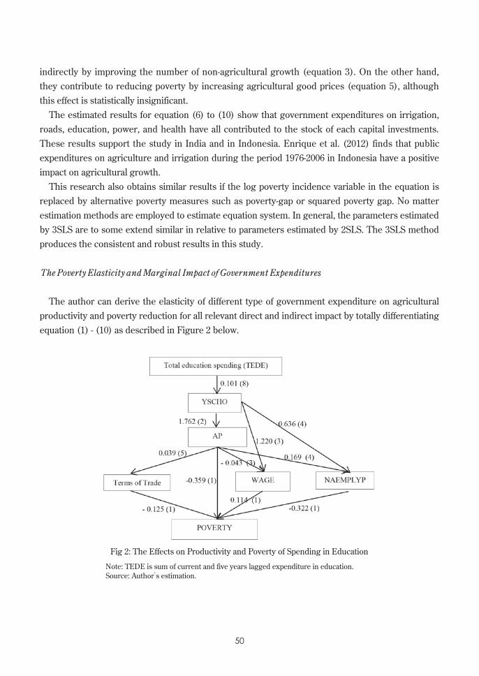
The Poverty Elasticity and Marginal Impact of Government Expenditures

The author can derive the elasticity of different type of government expenditure on agricultural

productivity and poverty reduction for all relevant direct and indirect impact by totally differentiating

equation (1) - (10) as described in Figure 2 below.

Note: TEDE is sum of current and five years lagged expenditure in education.Source: Author’s estimation.

Fig 2: The Effects on Productivity and Poverty of Spending in Education

5150

The calculation for the elasticity of education expenditure on agricultural productivity:

∂AP/∂EDE = (∂AP/∂YSCHO)(∂YSCHO /∂TEDE)

= 1.762 ＊ 0.101 = 0.178

This formula measures the direct impact of government spending in education on agricultural

productivity. By aggregating the total effects of all past government spending over the lag period,

the sum of marginal effects is obtained for any particular year. Similar formula in various types of

expenditure can be used and the results as shown in column 2 of Table 5.

While calculation for the total poverty effect of government spending on health:

∂P/∂EDE = (∂P/∂AP)(∂AP/∂YSCHO)(∂YSCHO/∂TEDE)

+ (∂P/∂TT)(∂TT/∂AP)(∂AP/∂YSCHO)(∂YSCHO/∂TEDE)

+ (∂P/∂WAGE)(∂WAGE/∂AP)(∂AP/∂YSCHO)(∂YSCHO/∂TEDE)

+ (∂P/∂NAEMPLYP)(∂NAEMPLYP/∂AP)(∂AP/∂YSCHO)(∂YSCHO/∂TEDE)

+ (∂P/∂WAGE)(∂WAGE/∂YSCHO)(∂YSCHO/∂TEDE)

+ (∂P/∂NAEMPLYP)(∂NAEMPLYP/∂YSCHO)(∂YSCHO/∂TEDE)

= - 0.082

The first term on the right side of the equation above measures the direct effect of increased

productivity on poverty attributed to the improved education investment. Terms 2, 3, and 4 are

the indirect effect of increased productivity through changes in prices, wages, and nonfarm

employment. Term 5 and 6 of the equation capture the direct effect of increased education

investment on poverty through higher wages and nonfarm employment opportunities. The total

effects on poverty of increased expenditure in power, irrigation, roads, and health can be similarly

derived as seen in column 4 of Table 5.

Table 5 shows the effect of different types of government spending on poverty and agricultural

productivity. Firstly, the elasticity of each type of government spending gives the percentage

change in poverty or productivity corresponding to a one ％ change in each spending types. This

Table 5: Poverty and Productivity Effects of Government Expenditures

ExpenditureElasticity Marginal Impact per 1 trillion Rp.

Number of Poor Reduced

Agri. Productivity Poverty Agri. Productivity Poverty per 10 billion Rp. SE SE ％ Point Rank ％ Point Rank People Rank

（1） （2） （3） （4） （5） （6） （7） （8） （9） （10） （11）Agriculture 0.254＊＊＊ 0.094 -0.108＊＊ 0.042 0.145 1 -0.073 1 -202.1 1Irrigation 0.001 0.012 -0.0004 0.005 0.009 3 -0.0036 4 -10.1 4Roads 0.005 0.019 -0.006 0.009 0.003 5 -0.004 3 -11.5 3Education 0.178＊＊ 0.084 -0.082＊ 0.044 0.015 2 -0.008 2 -21.5 2Power 0.006 0.009 -0.001 0.004 0.004 4 -0.001 5 -1.9 5Health -0.072＊＊ 0.034 0.013 0.013 -0.024 6 0.005 6 13.5 6

Notes: ‐＊), ＊＊), and ＊＊＊) indicate a significance at 10％ , 5％ , and 1％ respectively. ‐ Author uses the nonlinear combination procedure to compute estimated coefficients, associated standard errors, and

p-values expenditures with STATA application (Greene, 1993, p.187 and Cameron and Trivedi, 2009, p.332 and 396-397).Source: Author’s calculation based on estimation results.

5352

elasticity measures the relative productivity and poverty reducing benefits from additional spending.

Secondly, the marginal impact, measured in poverty and productivity for an additional trillion Rupiah

of government spending. The marginal impact is calculated by multiplying the elasticity by the ratio

of the poverty or productivity variable to the relevant spending item in the last period data and their

results as seen in column 6 and 8 of Table 5. It allows us to calculate the number of poor people who

would be raised above poverty line for one unit Rupiah of additional expenditure in each sector with

multiply their marginal impact by the number of poor people in the last period data

Government expenditure on agriculture (education) has the largest (second largest) significant

impact on poverty reduction as well as on productivity. The fact that the majority of poor people

living in rural areas and working mostly in agricultural sector. Therefore, agriculture expenditure

could be a powerful instrument to reduce poverty. This result is consistent with a study by Dartanto

and Nurkholis (2011) in which one of the determinants of poverty dynamics in Indonesia is

educational attainment. Comparing with previous study such as in India, Thailand, Vietnam, and

Uganda is that agricultural spending is the second largest significant impact on poverty reduction

after infrastructural spending such as roads spending or electric spending.

If the government increases spending in agriculture by one trillion Rupiah, the poverty rate

would be reduced by 0.073％ and the productivity would be increased 0.145％. Moreover, for every

additional 10 billion Rupiah in agricultural spending, 202 poor people would be reduced. Then 21

people (11 people) would be raised above poverty line if additional of 10 billion Rupiah is invested in

education (roads).

Government expenditures on irrigation, power, and roads have statistically insignificant positive

marginal impact on productivity with ranking third, fourth, and fifth respectively. Meanwhile,

they have marginal impact on poverty reduction with ranking fourth, fifth, and third respectively.

However, these types of spending do not have statistically significant productivity impacts and do

not contribute to long run poverty solution.

Spending in road has higher marginal impact on poverty reduction rather than on agricultural

productivity. Otherwise, expenditures in irrigation and power have higher marginal impact on

agricultural productivity rather than on poverty reduction. In general, all types of spending have

relatively the same ranking on productivity effect as well as on poverty reduction effect. This

indicates that there are limited trade-offs that arise among the achievements of this two objectives.

Those achievements can be interpreted as being complementary.

Spending on health has negative significantly effect on productivity and has negative insignificant

effect on poverty reduction. Investment on health could not directly increase the agricultural

productivity and also could not reduce the poverty, but this investment could increases percentage

of the number of non-agricultural employment. I conclude that the outcome of health expenditure is

less beneficial for the poor and more worthwhile for the non-poor.

5352

5. Conclusion

Using provincial level data from 2005 to 2014, a simultaneous equation system was developed to

estimate the direct and indirect effects of different types of government spending on poverty and

agricultural productivity in Indonesia. The empirical findings in this paper can be summarized as

follows. Government expenditures on agriculture, education, roads, irrigation, and power have all

contributed to agricultural productivity and contributed to poverty reduction, but their effects vary.

Government expenditure on agriculture has the largest impact on agricultural productivity and poverty

reduction, followed by education, irrigation, roads, and power spending. However, only agricultural

and education expenditures significantly impacts on productivity and poverty reduction. Generally, the

achievements of each public spending for these two goals can be interpreted as being complementary.

Thus, there are limited trade-offs among their effects on agricultural productivity and poverty rate.

In contrast, over the analyzed period, government spending on health has negative significantly

impact on agricultural productivity and as a result could not reduce poverty. Outcome of this health

expenditure is slightly pro-poor that living in remote area and working in agricultural sector. Policy

makers with limited budget need to allocate resources efficiently. To alleviate poverty in long term,

the Government of Indonesia should increase its spending on agriculture and education. These

expenditures do not only promotes higher productivity levels in the agricultural sector, but also,

indirectly and directly see a high marginal impact on poverty reduction.

Thus, in order to promote the agricultural productivity, the Government of Indonesia should

prioritize investment in education and allocate more in agricultural spending. Simultaneously, the

poverty rate can be alleviated through improving agricultural productivity and creating non-farm

employment.

6. Acknowledgement

I gratefully appreciated the financial support from the Haraguchi Memorial Research Fund who

gave me the opportunity to conduct this research. I would like to thank the 15th East Asian Economic

Association (EAEA) Conference members in Bandung, Indonesia for their helpful comments and

panel discussions, without which the present study could not have been completed.

（Received 27th April, 2017） （Accepted 29th July, 2017）

ReferencesBird, Kelly, and Chris Manning. (2008). “Minimum Wage and Povery in a Developing Country: Simulation

from Indonesia’s Household Survey.” World Development, Vol 36, No.5, pp. 916-933.

Cameron A. Colin and Pravin K. Trivedi. (2009). Microeconometrics Using Stata. Texas: A Stata Press.

Dartanto, Teguh. (2013). “Why is Growth Growth Less Inclusive in Indonesia.” Institute for Economic and

Social Research (LPEM), University of Indonesia. Personal Munich RePEc Archive (MPRA) Paper No.

PB54

65136. https://mpra.ub.uni-muenchen.de/65136/ (May 3,2016).

Dartanto, Teguh and Nurkholis. (2013). “Finding Out the Determinants of Poverty Dinamics in Indonesia:

Evidence from Panel Data.” Bulletin of Indonesian Economics Studies, Vol 49-Issue 1.

Fan, Shenggen; Linxiu Zhang; and Xiaobo Zhang. (2004).“Reform, Investment, and Poverty Government in

Rural China”. Journal of Economic Development and Cultural Change Vol. 52(2): 395-421.

Fan, S., and N. Rao. (2008).“Public Spending, Growth, and Rural Poverty.” In Public Expenditures, Growth, and

Poverty: Lessons from Developing Countries, Washington, D.C.: The Johns Hopkins University Press.

Fan, Shenggen; Peter Hazell; and Sukhadeo Thorat. (2000).“Government Spending, Growth, and Poverty in

Rural India.” American Journal of Agricultural Economic, 82(4), 1038-1051. Fan, Shenggen; P.L. Huong;

and T.Q. Long. (2004). Government Spending and Poverty in Vietnam. World Bank Project Report. IFPRI.

Washington D.C.

Fan, Shenggen; Somchai Jitsuchon; and Methakunnavut Nuntaporn. (2004). “The Importance of Public

Investment for Reducing Rural Poverty in Middle-Income Countries: The Case of Thailand.” Discussion

Paper No.7. IFPRI. Washington D.C.

Foster Andrew D. and Mark R. Rosenzweig. (2004).“Agricultural Productivity Growth, Rural Economic

Diversity, and Economic Reform, India 1970-2000.” Journal of Economic Development and Cultural Change,

Vol. 52 No.3 pp. 509-542.

Greene, W.H. (1993). Econometric Analysis. Englewood Cliffs New Jersey: Practice Hall.

Gupta, Sanjev, Benedict Clements, Emanuele Baldacci and Carlos Mulas-Granados. (2005). “Fiscal Policy,

Expenditure Composition and Growth in Low Income Countries.” Journal of International Money and

Finance, Vol.24, 441-46.

Hasan, Rana, and M.G. Quibria. (2004). “Industry Matters for Poverty: A Critique of Agricultural Fundamentalism.” Kyklos International Reviews for Social Sciences. Wiley online library. Vol. 57, No. 2, 253-264.

Indriawan, Yudi, and Muhyiddin. (2007). “Government Size and Growth: Evience from Indonesia.” Journal of

Development Planning, Ed. 03-04/XII.

Lanjouw, Peter et. al. (2001). “Education, and Health in Indonesia: Who Benefits from Public Spending?” World Bank Policy Research Working Paper No.2739. https://papers.ssrn.com/sol3/papers.cfm?abstract_

id=634451. (May 30, 2016)

Ravallion, M., and G. Datt. (1996). How Important to India’s Poor is The Sectoral Composition of Economic

Growth. World Bank Economic Reviews, 10, 1-25

Statistics Indonesia, Statistical Yearbook of Indonesia in various years from 2009-2015. http://www.bps.go.id/

index.php/Publikasi (May 5, 2016)

Suryahadi, Asep, Daniel Suryadarma, and Sudarno Sumarto. (2009). “Economic Growth and Poverty Reduction

in Indonesia: The Effect of Location and Sectoral Component of Growth.” Journal of Development Economics,

Vol 89.

World Bank. (2015). Indonesia Database for Policy and Economic Research. http://data.worldbank.org/data-

catalog/indonesia-database-for-policy-and-economic-research (Juni 17, 2015).