Learning Discriminative Model Prediction for Tracking

Goutam Bhat∗ Martin Danelljan∗ Luc Van Gool Radu Timofte

CVL, ETH Zurich, Switzerland

Abstract

The current strive towards end-to-end trainable com-puter vision systems imposes major challenges for the taskof visual tracking. In contrast to most other vision problems,tracking requires the learning of a robust target-specific ap-pearance model online, during the inference stage. To beend-to-end trainable, the online learning of the target modelthus needs to be embedded in the tracking architecture it-self. Due to these difficulties, the popular Siamese paradigmsimply predicts a target feature template. However, such amodel possesses limited discriminative power due to its in-ability of integrating background information.

We develop an end-to-end tracking architecture, capableof fully exploiting both target and background appearanceinformation for target model prediction. Our architecture isderived from a discriminative learning loss by designing adedicated optimization process that is capable of predictinga powerful model in only a few iterations. Furthermore, ourapproach is able to learn key aspects of the discriminativeloss itself. The proposed tracker sets a new state-of-the-arton 6 tracking benchmarks, achieving an EAO score of 0.440on VOT2018, while running at over 40 FPS.

1. Introduction

Generic object tracking is the task of estimating the stateof an arbitrary target in each frame of a video sequence. Inthe most general setting, the target is only defined by its ini-tial state in the sequence. Most current approaches addressthe tracking problem by constructing a target model, capa-ble of differentiating between the target and background ap-pearance. Since target-specific information is only availableat test-time, the target model cannot be learned in an of-fline training phase, as in for instance object detection. In-stead, the target model must be constructed during the infer-ence stage itself by exploiting the target information givenat test-time. This unconventional nature of the visual track-ing problem imposes significant challenges when pursuing

∗Both authors contributed equally.

Image Siamese based OursFigure 1. Visualization of confidence maps provided by the tar-get model obtained using i) a Siamese based approach (middle),and ii) Our discriminative approach (right). The red box indicatesthe target object in each image (left). The model predicted in aSiamese fashion, using only target appearance, struggles to dis-tinguish the target from distractor objects in the background. Incontrast, our approach generates target models with superior dis-criminative power, that are robust to background distractors.

an end-to-end learning solution.The aforementioned problems have been most success-

fully addressed by the Siamese learning paradigm [34, 1,21]. These approaches first learn a feature embedding,where the similarity between two image regions is com-puted by a simple cross-correlation. Tracking is then per-formed by finding the image region most similar to the tar-get template. In this setting, the target model simply cor-responds to the template features extracted from the targetregion. Consequently, the tracker can easily be trained end-to-end using pairs of annotated images.

Despite its recent success, the Siamese learning frame-work suffers from severe limitations. Firstly, Siamese track-ers only utilize the target appearance when inferring themodel. This completely ignores background appearanceinformation, which is crucial for discriminating the targetfrom similar objects in the scene (see figure 1). Secondly,the learned similarity measure is not necessarily reliable forobjects that are not included in the offline training set, lead-

1

arX

iv:1

904.

0722

0v1

[cs

.CV

] 1

5 A

pr 2

019

ing to poor generalization. Thirdly, the Siamese formulationdoes not provide a powerful model update strategy. Instead,state-of-the-art approaches resort to simple template averag-ing [40]. These limitations result in inferior robustness [18]compared to other state-of-the-art tracking approaches.

In this work, we introduce an alternative tracking ar-chitecture, trained in an end-to-end manner, that directlyaddresses all aforementioned limitations. In our design,we take inspiration from the discriminative learning proce-dures that have been successfully applied in recent track-ers [26, 7, 4]. Our approach is based on a target modelprediction network, which is derived from a discriminativelearning loss by applying an iterative optimization proce-dure. The architecture is carefully designed to enable ef-fective end-to-end training, while maximizing the discrim-inative power of the predicted model. This is achieved byensuring a minimal number of optimization steps throughtwo key design choices. First, we employ a steepest descentbased methodology that computes an optimal step lengthin each iteration. Second, we integrate a module that ef-fectively initializes the target model. Furthermore, we in-troduce significant flexibility into our final architecture bylearning the discriminative loss itself.

Our entire discriminative tracking architecture, alongwith the backbone feature extractor, is trained using anno-tated tracking sequences by minimizing the prediction erroron future frames. We perform comprehensive experimentson seven tracking benchmarks: NFS [9], UAV123 [24],OTB100 [37], TrackingNet [25], LaSOT [8], GOT10k [13]and VOT2018 [18]. Our approach achieves state-of-the-artresults on all seven datasets, while running at over 40 FPS.We further provide an extensive experimental analysis ofthe proposed discriminative learning architecture, showingthe impact of each component.

2. Related WorkGeneric object tracking has undergone astonishing

progress in recent years, with the development of a vari-ety of approaches. Recently, methods based on Siamesenetworks [1, 34, 21] have received much attention due totheir end-to-end training capabilities and high efficiency.The name derives from the deployment of a Siamese net-work architecture in order to learn a similarity metric of-fline. Bertinetto et al. [1] utilize a fully-convolutional ar-chitecture for similarity prediction, thereby attaining hightracking speeds of over 100 FPS. Wang et al. [36] learn aresidual attention mechanism to adapt the tracking model tothe current target. Li et al. [21] employ a region proposalnetwork [30] to obtain accurate bounding boxes.

A key limitation in Siamese approaches is their inabil-ity to incorporate information from the background regionor previous tracked frames into the model prediction. Afew recent attempts aims to address these issues. Guo et

al. [10] learn a feature transformation to handle the targetappearance changes and to suppress background. Further,Zhu et al. [40] handle background distractors by subtract-ing corresponding image features from the target templateduring online tracking. Despite these attempts, the Siamesetrackers are yet to reach high level of robustness attained bystate-of-the-art trackers employing online learning [18].

In contrast to Siamese methods, another family of track-ers [26, 5, 4] learn a discriminative classifier online to dis-tinguish the target object from the background. These ap-proaches can effectively utilize background information,thereby achieving impressive robustness on multiple track-ing benchmarks [37, 18]. However, these methods rely onmore complicated online learning procedures that cannotbe easily formulated in an end-to-end learning framework.Thus, these approaches are often restricted to features ex-tracted from deep networks pre-trained for image classifi-cation [7, 23] or hand-crafted alternatives [6].

A few recent works aim to formulate existing discrim-inative trackers as a neural network component in orderto benefit from end-to-end training on tracking data. Val-madre et al. [35] integrate the single-sample closed-formsolution of the correlation filter (CF) [12] into a deep net-work. However, such a simple CF model has poor dis-criminative power, providing little gains over the Siamesebaseline. Yao et al. [39] unroll the ADMM iterations inBACF [16] tracker to learn the feature extractor along withsome tracking hyper-parameters in a complex multi-stagetraining procedure. The BACF model learning is howeverrestricted to the single-sample variant of the Fourier-domainCF formulation. Such a formulation cannot exploit multi-ple samples, requiring ad-hoc linear combination of filtersfor model adaption. Park et al. [28] develop a meta-learningframework employing an initial, target independent model,which is then refined using gradient descent with learnedstep-lengths. However, this strategy is only suitable for aninitial adaption of the model and does not improve whenapplied in an iterative manner. This is due to the fact that itis not possible to learn constant step-lengths that accommo-date both fast initial adaption and optimal convergence.

3. MethodIn this work, we develop a discriminative model pre-

diction architecture for visual tracking. As in Siamesetrackers, our approach benefits from end-to-end training.However, unlike Siamese, our architecture can fully exploitbackground information and provides natural and powerfulmeans of updating the target model with new data. Ourmodel prediction network is derived from two main princi-ples: (i) A discriminative loss function capable of learning arobust target model; and (ii) a powerful optimization strat-egy ensuring rapid convergence. By such careful design,our architecture can predict the target model in only a few

Backbone Cls Feat

Model Initializer

Initial Model f

Model Optimizer

ConvCls

Feat

Update Model f

Trai

ning

Set

Score Prediction Te

st F

ram

e

Backbone

Final Model f

Feature Extractor F Model Predictor D

(0)

(i)

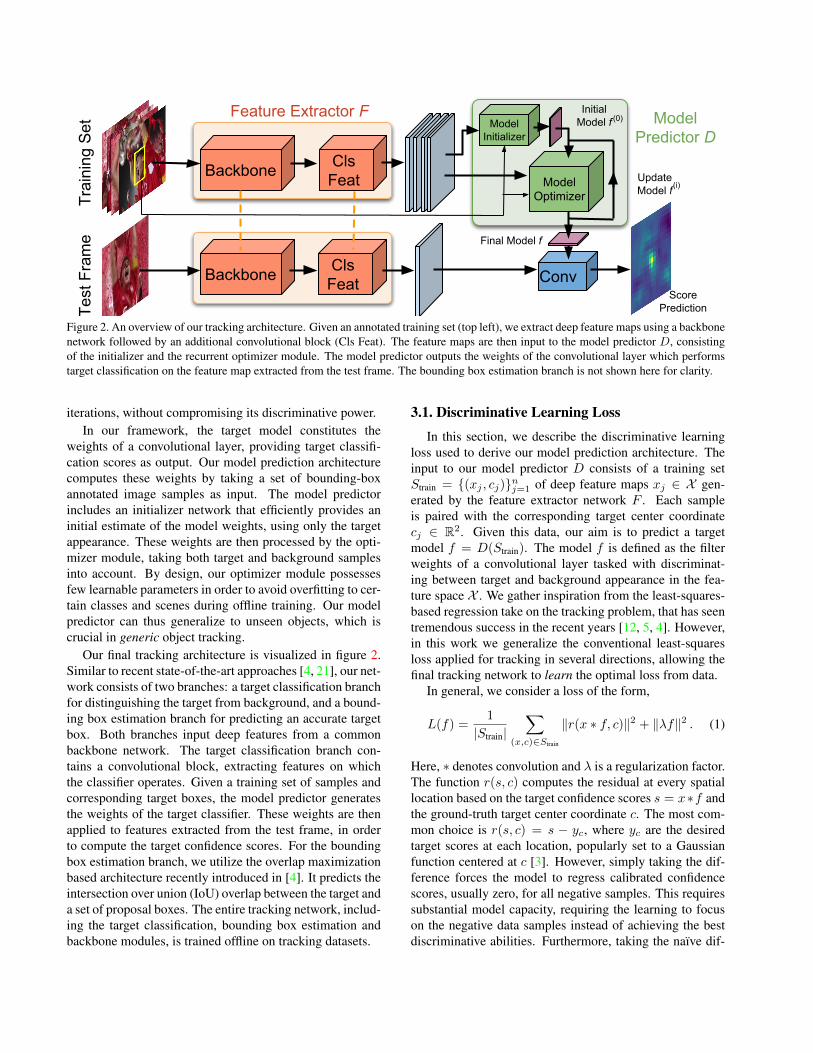
Figure 2. An overview of our tracking architecture. Given an annotated training set (top left), we extract deep feature maps using a backbonenetwork followed by an additional convolutional block (Cls Feat). The feature maps are then input to the model predictor D, consistingof the initializer and the recurrent optimizer module. The model predictor outputs the weights of the convolutional layer which performstarget classification on the feature map extracted from the test frame. The bounding box estimation branch is not shown here for clarity.

iterations, without compromising its discriminative power.In our framework, the target model constitutes the

weights of a convolutional layer, providing target classifi-cation scores as output. Our model prediction architecturecomputes these weights by taking a set of bounding-boxannotated image samples as input. The model predictorincludes an initializer network that efficiently provides aninitial estimate of the model weights, using only the targetappearance. These weights are then processed by the opti-mizer module, taking both target and background samplesinto account. By design, our optimizer module possessesfew learnable parameters in order to avoid overfitting to cer-tain classes and scenes during offline training. Our modelpredictor can thus generalize to unseen objects, which iscrucial in generic object tracking.

Our final tracking architecture is visualized in figure 2.Similar to recent state-of-the-art approaches [4, 21], our net-work consists of two branches: a target classification branchfor distinguishing the target from background, and a bound-ing box estimation branch for predicting an accurate targetbox. Both branches input deep features from a commonbackbone network. The target classification branch con-tains a convolutional block, extracting features on whichthe classifier operates. Given a training set of samples andcorresponding target boxes, the model predictor generatesthe weights of the target classifier. These weights are thenapplied to features extracted from the test frame, in orderto compute the target confidence scores. For the boundingbox estimation branch, we utilize the overlap maximizationbased architecture recently introduced in [4]. It predicts theintersection over union (IoU) overlap between the target anda set of proposal boxes. The entire tracking network, includ-ing the target classification, bounding box estimation andbackbone modules, is trained offline on tracking datasets.

3.1. Discriminative Learning Loss

In this section, we describe the discriminative learningloss used to derive our model prediction architecture. Theinput to our model predictor D consists of a training setStrain = {(xj , cj)}nj=1 of deep feature maps xj ∈ X gen-erated by the feature extractor network F . Each sampleis paired with the corresponding target center coordinatecj ∈ R2. Given this data, our aim is to predict a targetmodel f = D(Strain). The model f is defined as the filterweights of a convolutional layer tasked with discriminat-ing between target and background appearance in the fea-ture space X . We gather inspiration from the least-squares-based regression take on the tracking problem, that has seentremendous success in the recent years [12, 5, 4]. However,in this work we generalize the conventional least-squaresloss applied for tracking in several directions, allowing thefinal tracking network to learn the optimal loss from data.

In general, we consider a loss of the form,

L(f) =1

|Strain|∑

(x,c)∈Strain

‖r(x ∗ f, c)‖2 + ‖λf‖2 . (1)

Here, ∗ denotes convolution and λ is a regularization factor.The function r(s, c) computes the residual at every spatiallocation based on the target confidence scores s = x∗f andthe ground-truth target center coordinate c. The most com-mon choice is r(s, c) = s − yc, where yc are the desiredtarget scores at each location, popularly set to a Gaussianfunction centered at c [3]. However, simply taking the dif-ference forces the model to regress calibrated confidencescores, usually zero, for all negative samples. This requiressubstantial model capacity, requiring the learning to focuson the negative data samples instead of achieving the bestdiscriminative abilities. Furthermore, taking the naıve dif-

ference does not address the problem of data imbalance be-tween target and background.

To alleviate the latter issue of data imbalance, we use aspatial weight function vc. The subscript c indicates the de-pendence on the center location of the target, as detailed insection 3.4. To accommodate the first issue, we modify theloss following the philosophy of Support Vector Machines.We employ a hinge-like loss in r, clipping the scores at zeroas max(0, s) in the background region. The model is thusfree to predict large negative values for easy samples in thebackground without increasing the loss. For the target re-gion on the other hand, we found it disadvantageous to addan analogous hinge loss max(0, 1−s). Although contradic-tory at a first glance, this behavior can be attributed to thefundamental asymmetry between the target and backgroundclass, partially due to the numerical imbalance. Moreover,accurately calibrated target confidences are indeed advanta-geous in the tracking scenario, e.g. for detecting target loss.We therefore desire the properties of standard least-squaresregression in the target neighborhood.

To accommodate the advantages of both least-squares re-gression and the hinge loss, we define the residual function,

r(s, c) = vc · (mcs+ (1−mc) max(0, s)− yc) . (2)

The target region is defined by the mask mc, having val-ues in the interval mc(t) ∈ [0, 1] at each spatial locationt ∈ R2. Again, the subscript c indicate the dependence onthe target center coordinate. The formulation in (2) is capa-ble of continuously changing the behavior of the loss fromstandard least squares regression to a hinge loss dependingon the image location relative to the target center c. Settingmc ≈ 1 at the target and mc ≈ 0 in the background regionyields the desired behavior described above. However, howto optimally setmc is not clear, in particular at the transitionregion between target and background. While the classicalstrategy is to manually set the mask parameters using trialand error, our end-to-end formulation allows us to learn themask in a data-driven manner. In fact, as detailed in sec-tion 3.4, our approach learns all free parameters in the loss:the target mask mc, the spatial weight vc, the regularizationfactor λ, and even the regression target yc itself.

3.2. Optimization-Based Architecture

Here, we derive the network architecture D that predictsthe filter f = D(Strain) by implicitly minimizing the error(1). The network is designed by formulating an optimiza-tion procedure. From eqs. (1) and (2) we can easily derivea closed-form expression for the gradient of the loss ∇Lwith respect to the filter f .2 The straight-forward option isto then employ gradient descent using a step length α,

f (i+1) = f (i) − α∇L(f (i)) . (3)2See supplementary material (section S1) for details.

However, we found this simple approach to be insufficient,even if the learning rate α (either a scalar or coefficient-specific) is learned by the network itself (see section 4.1). Itexperiences slow adaption of the filter parameters f , requir-ing a vast increase in the number of iterations. This harmsefficiency and complicates offline learning.

The slow convergence of gradient descent is largely dueto the constant step length α, which does not depend on dataor the current model estimate. We solve this issue by deriv-ing a more elaborate optimization approach, requiring onlya handful of iterations to predict a strong discriminative fil-ter f . The core idea is to compute the step length α basedon the steepest descent methodology, which is a commonoptimization technique [27, 32]. We first approximate theloss with a quadratic function at the current estimate f (i),

L(f) ≈ L(f) =1

2(f − f (i))TQ(i)(f − f (i))+ (4)

(f − f (i))T∇L(f (i)) + L(f (i)) .

Here, the filter variables f and f (i) are seen as vectors andQ(i) is positive definite square matrix. The steepest descentthen proceeds by finding the step length α that minimizesthe approximate loss (4) in the gradient direction (3). Thisis found by solving d

dα L(f (i) − α∇L(f (i))

)= 0, as

α =∇L(f (i))T∇L(f (i))

∇L(f (i))TQ(i)∇L(f (i)). (5)

In steepest descent, the formula (5) is used to compute thescalar step length α in each iteration of the filter update (3).

The quadratic model (4), and consequently the resultingstep length (5), depends on the choice of Q(i). For exam-ple, by using a scaled identity matrix Q(i) = 1

β I we re-trieve the standard gradient descent algorithm with a fixedstep length α = β. On the other hand, we can now integratesecond order information into the optimization procedure.The most obvious choice is setting Q(i) = ∂2L

∂f2 (f (i)) to theHessian of the loss (1), which corresponds to a second orderTaylor approximation (4). For our least-squares formula-tion (1) however, the Gauss-Newton method [27] providesa powerful alternative, with significant computational bene-fits since it only involves first-order derivatives. We thus setQ(i) = (J (i))TJ (i), where J (i) is the Jacobian of the resid-uals at f (i). In fact, neither the matrix Q(i) or Jacobian J (i)

need to be constructed explicitly, but rather implementedas a sequence of neural network operations. See the sup-plementary material (section S2) for details. Algorithm 1describes our target model predictor D. Note that our op-timizer module can easily be employed for online modeladaption as well. This is achieved by continuously extend-ing the training set Strain with new samples from the previ-ously tracked frames. The optimizer module is then appliedon this extended training set, using the current target modelas the initialization f (0).

Algorithm 1 Target model prediction D.Input: Samples Strain = {(xj , cj)}nj=1, iterations Niter

1: f (0) ← ModelInit(Strain) # Initialize filter (sec 3.3)2: for i = 0, . . . , Niter − 1 do # Optimizer module loop3: ∇L(f (i))← FiltGrad(f (i), Strain) # Using (1)-(2)4: h← J (i)∇L(f (i)) # Apply Jacobian of (2)5: α← ‖∇L(f (i))‖2/‖h‖2 # Compute step length (5)6: f (i+1) ← f (i) − α∇L(f (i)) # Update filter7: end for

3.3. Initial filter prediction

To further reduce the number of optimization recursionsrequired inD, we introduce a small network module trainedto predict an initial model estimate f (0). Our initializer net-work consists of a convolutional layer followed by a pre-cise ROI pooling [14]. The latter extracts features from thetarget region and pools them to the same size as the tar-get model f . The pooled feature maps are then averagedover all the samples in Strain to obtain the initial model f (0).As in Siamese trackers, this approach only utilizes the tar-get appearance. However, rather than predicting the finalmodel, our initializer network is tasked with only providinga reasonable initial estimate, which is then processed by theoptimizer module to provide the final discriminative model.

3.4. Learning the Discriminative Loss

Here, we describe how the free parameters in the resid-ual function (2), defining the discriminative loss (1), arelearned. Our residual function includes the label confidencescores yc, the spatial weight function vc and the target maskmc. While such variables are constructed by hand in currentdiscriminative trackers, our approach in fact learns thesefunctions from data. We parametrize them based on the dis-tance from the target center. This is motivated by the radialsymmetry of the problem, where the direction to the sam-ple location relative to the target is of little significance. Onthe other hand, the distance to the sample location plays acrucial role, especially in the transition from target to back-ground. Thus, we parameterize yc, mc and vc using radialbasis functions ρk and learn their coefficients φk. For in-stance, the label yc at position t ∈ R2 is given by

yc(t) =

N−1∑k=0

φykρk(‖t− c‖) . (6)

We use triangular basis functions ρk, defined as

ρk(d) =

{max(0, 1− |d−k∆|

∆ ), k < N − 1

max(0,min(1, 1 + d−k∆∆ )), k = N − 1

(7)

The above formulation corresponds to a continuous piece-wise linear function with a knot displacement of ∆. Note

0 1 2 3 4 5 6 7 8 9 10 11 12Distance from target center

0

0.5

1

1.5

Val

ue

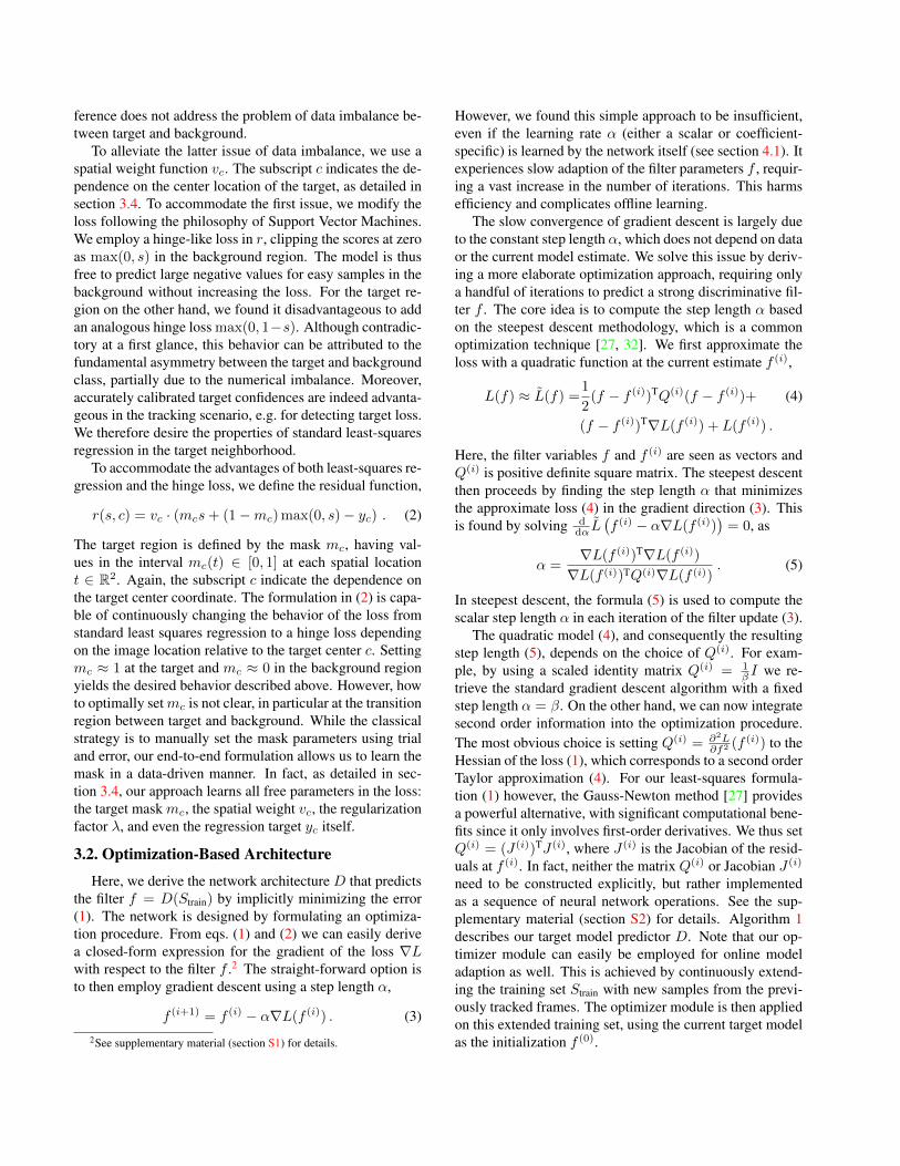
Figure 3. Plot of the learned regression label (yc), target mask(mc), and spatial weight (vc). The markers show the knot loca-tions. The initialization of each quantity is shown in dotted lines.

that the final case k = N−1 represents all locations that arefar away from the target center and thus can be treated iden-tically. We use a small ∆ to enable accurate representationof the regression label at the target-background transition.The functions vc and mc are parameterized analogously us-ing coefficients φvk and φmk respectively in (6). For the tar-get mask mc, we constrain the values to the interval [0, 1]by passing the output from (6) through a Sigmoid function.

We useN = 10 basis functions and set the knot displace-ment to ∆ = 0.5 in the resolution of the deep feature spaceX . For offline training, the regression label yc is initializedto the same Gaussian zc used in the offline classificationloss, described in section 3.5. The weight function vc is ini-tialized to constant vc(t) = 1. Lastly, we initialize the targetmask mc using a scaled tanh function. The coefficients φk,along with λ, are learned as part of the model predictionnetwork D (see section 3.5). The initial and learned valuesfor yc, mc and vc are visualized in figure 3. Notably, ournetwork learns to increase the weight vc at the target centerand reduce it in the ambiguous transition region.

3.5. Offline training

Here, we describe our offline training procedure. InSiamese approaches, the network is trained with imagepairs, using one image to predict the target template andthe other for evaluating the tracker. In contrast, our modelprediction network D inputs a set Strain of multiple datasamples from the sequence. To better exploit this advan-tage, we train our full tracking architecture on pairs of sets(Mtrain,Mtest). Each set M = {(Ij , bj)}Nframes

j=1 consists ofimages Ij paired with their corresponding target boundingboxes bj . The target model is predicted using Mtrain andthen evaluated on the test frames Mtest. Uniquely, our train-ing allows the model predictor D to learn how to better uti-lize multiple samples. The sets are constructed by samplinga random segment of length Tss in the sequence. We thenconstruct Mtrain and Mtest by sampling Nframes frames eachfrom the first and second halves of the segment respectively.

Given the pair (Mtrain,Mtest), we first pass the imagesthrough the backbone feature extractor to construct the trainStrain and test Stest samples for our target model. Formally,the train set is obtained as Strain = {(F (Ij), cj) : (Ij , bj) ∈

Mtrain}, where cj is the center coordinate of the box bj . Thisis input to the target predictor f = D(Strain). The aim is topredict a model f that is discriminative and that generalizeswell to future unseen frames. We therefore only evaluatethe predicted model f on the test samples Stest, obtainedanalogously using Mtest. Following the discussion in sec-tion 3.1, we compute the regression errors using a hinge forthe background samples,

`(s, z) =

{s− z , z > T

max(0, s) , z ≤ T. (8)

Here, the threshold T defines the target and background re-gion based on the label confidence value z. For the targetregion z > T we take the difference between the predictedconfidence score s and the label z, while we only penalizepositive confidence values for the background z ≤ T .

The total target classification loss is computed as themean squared error (8) over all test samples. However, in-stead of only evaluating the final target model f , we averagethe loss over the estimates f (i) obtained in each iteration iby the optimizer (see alg. 1). This introduces intermedi-ate supervision to the target prediction module, benefitingtraining convergence. Furthermore, we do not aim to trainfor a specific number of recursions, but rather be free to setthe desired number of optimization recursions online. It isthus natural to evaluate each iterate f (i) equally. The targetclassification loss used for offline training is given by,

Lcls =1

Niter

Niter∑i=0

∑(x,c)∈Stest

∥∥∥`(x ∗ f (i), zc)∥∥∥2

. (9)

Here, regression label zc is set to a Gaussian function cen-tered as the target c. Note that the output f (0) from the filterinitializer (section 3.3) is also included in the above loss.Although not denoted explicitly to avoid clutter, both x andf (i) in (9) depend on the parameters of the feature extrac-tion network F . The model iterates f (i) additionally dependon the parameters in the model predictor network D.

For bounding box estimation, we train the IoU-Net [14]based architecture proposed in [4], employing features fromthe same backbone network used for target classification.The training procedure in [4] is extended to image sets bycomputing the modulation vector on the first frame inMtrainand sampling proposal boxes from all images in Mtest. Thebounding box estimation loss Lbb is computed as the meansquared error between the predicted IoU overlaps in Mtestand the actual overlaps with the annotated boxes. We trainthe full tracking architecture by combining this with the tar-get classification loss (9) as Ltot = βLcls + Lbb.Training details: Our training procedure is simple, re-quiring only a single phase where the entire architecture islearned jointly. The backbone network is initialized with the

ImageNet weights. We use the training splits of the Track-ingNet [25], LaSOT [8], GOT10k [13] and COCO [22]datasets. We train for 50 epochs by sampling 20,000 videosper epoch, giving a total training time of less than 24 hourson a single Nvidia TITAN X GPU. We use ADAM [17] withlearning rate decay of 0.2 every 15th epoch. The target clas-sification loss weight is set to β = 102 and we useNiter = 5optimizer module recursions in (9) during training.

The image patches in (Mtrain,Mtest) are extracted bysampling a random translation and scale relative to the tar-get annotation. We set the base scale to 5 times the targetsize to incorporate significant background information. Foreach sequence, we sampleNframes = 3 test and train frames,using a segment length of Tss = 60. The label scores zc areconstructed using a standard deviation of 1/4 relative to thebase target size, and we use T = 0.05 for the regressionerror (8). We employ the ResNet architecture for the back-bone. For the model predictor D, we use features extractedfrom the third block, having a spatial stride of 16. We setthe kernel size of the target model f to 4× 4.

3.6. Online tracking

Given the first frame with annotation, we employ dataaugmentation strategies [2] to construct an initial set Straincontaining 15 samples. The target model is then obtainedusing our discriminative model prediction architecture f =D(Strain). For the first frame, we employ 10 steepest de-scent recursions, after the initializer module. Our approachallows the target model to be easily updated by adding anew training sample to Strain whenever the target is pre-dicted with sufficient confidence. We ensure a maximummemory size of 50 by discarding the oldest sample. Duringtracking, we refine the target model f by performing twooptimizer recursions every 20 frames, or a single recursionwhenever a distractor peak is detected. Bounding box esti-mation is performed using the same settings as in [4].

4. ExperimentsOur approach is implemented in Python using PyTorch.

On a single Nvidia GTX 1080 GPU, we achieve a trackingspeed of 57 FPS when employing ResNet-18 as backboneand 43 FPS for ResNet-50. Detailed results are provided inthe supplementary material (section S3–S6). The completecode for training and inference will be made available athttps://github.com/visionml/pytracking.

4.1. Baseline Analysis

Here, we perform an extensive analysis of the proposedmodel prediction architecture. Experiments are performedon a combined dataset containing the entire OTB-100 [37],NFS (30 FPS version) [9] and UAV123 [24] datasets. Thispooled dataset contains 323 diverse videos to enable thor-ough analysis. The trackers are evaluated using the AUC

Init GD SD

AUC 58.2 61.6 63.8

Table 1. Analysis of different model prediction architectures onthe combined OTB-100, NFS and UAV123 datasets. The architec-ture using only the target information for model prediction (Init)achieves an AUC score of 58.2%. The proposed steepest descentbased architecture (SD) provides the best results, outperformingthe gradient descent method (GD) by over 2.2% AUC score.

SD +Init +FT +Cls +Loss

AUC 58.7 60.0 62.6 63.3 63.8

Table 2. Analysis of the impact of initializer module (+Init), train-ing the backbone (+FT), using extra conv. block (+Cls) and offlinelearning of the loss (+Loss), by incrementally adding them one ata time. The baseline SD constitutes our steepest descent basedoptimizer module along with ResNet-18 pre-trained on ImageNet.

[37] metric. Due to the stochastic nature of the tracker, wealways report the average AUC score over 5 runs. We em-ploy ResNet-18 as the backbone network for this analysis.Impact of optimizer module: We compare our proposedmethod, utilizing the steepest descent (SD) based archi-tecture, with two alternative model prediction networks.Init: Here, we only use the initializer module to predictthe final target model, which corresponds to removing theoptimizer module in our approach. Thus, similar to theSiamese approaches, only target appearance informationis used for model prediction, while background informa-tion is discarded. GD: In this approach, we replace steep-est descent with the gradient descent (GD) algorithm usinglearned coefficient-wise step-lengths α in (3). All networksare trained using the same settings. The results for this anal-ysis are shown in table 1.

The model predicted by the initializer network, whichuses only target information, achieves an AUC score of58.2%. The gradient descent approach, which can exploitbackground information, provides a substantial improve-ment, achieving an AUC score of 61.6%. This highlightsthe importance of employing discriminative learning formodel prediction. Our steepest descent approach obtainsthe best results, outperforming GD by 2.2%. This is dueto the superior convergence properties of steepest descent,important for offline learning and fast online tracking.Analysis of model prediction architecture: Here, we an-alyze the impact of key aspects of the proposed discrimi-native learning architecture, by incrementally adding themone at a time. The results are shown in table 2. The baselineSD constitutes our steepest descent based optimizer modulealong with the ImageNet pre-trained ResNet-18 network.That is, similar to the current state-of-the-art discriminativeapproaches, we do not fine-tune the backbone. Instead oflearning the discriminative loss, we employ the regressionerror (8) in the optimizer module. This baseline approach

No update Model averaging Ours

AUC 61.7 61.7 63.8

Table 3. Comparison of different model update strategies on thecombined OTB-100, NFS and UAV123 datasets.

DRT RCO UPDT DaSiam- MFT LADCF ATOM SiamRPN++ DiMP-18 DiMP-50[33] [18] [2] RPN [40] [18] [38] [4] [20]

EAO 0.356 0.376 0.378 0.383 0.385 0.389 0.401 0.414 0.402 0.440Robustness 0.201 0.155 0.184 0.276 0.140 0.159 0.204 0.234 0.182 0.153Accuracy 0.519 0.507 0.536 0.586 0.505 0.503 0.590 0.600 0.594 0.597

Table 4. State-of-the-art comparison on the VOT2018 dataset interms of expected average overlap (EAO), accuracy and robust-ness. Our approach, using ResNet-50 backbone (DiMP-50), out-performs the previous methods in terms of EAO.

achieves an AUC score of 58.7%. By adding the modelinitializer module (+Init), we achieve a significant gain of1.3% in AUC score. Further training the entire network, in-cluding backbone feature extractor, (+FT) leads to a majorimprovement of 2.6% in AUC score. This demonstrates theadvantages of learning discriminative features suitable fortracking, and possessing the ability of end-to-end learning.Using an additional convolutional block to extract classifi-cation specific features (+Cls) yields a further improvementof 0.7% AUC score. Finally, learning the discriminativeloss (2) itself (+Loss), as described in section 3.4, improvesthe AUC score by another 0.5%. This shows the benefit oflearning the implicit online loss by maximizing the gener-alization capabilities of the model on future frames.Impact of online model update: Here, we analyze the im-pact of updating the target model online, using informationfrom previous tracked frames. We compare three differentmodel update strategies. i) No update: The model is notupdated during tracking. Instead, the model predicted inthe first frame by our model predictor D, is employed forthe entire sequence. ii) Model averaging: In each frame,the target model is updated using the linear combination ofthe current and newly predicted model, as commonly em-ployed in tracking [12, 35, 16]. iii) Ours: The target modelis obtained using the training set constructed online, as de-scribed in section 3.6. The results are shown in table 3. Thenaıve model averaging fails to improve over the baselinemethod with no updates. In contrast, our approach obtainsa significant gain of about 2% in AUC score over both meth-ods. These results indicate that our approach can effectivelyadapt the target model online.

4.2. State-of-the-art Comparison

We compare our proposed approach DiMP with thestate-of-the-art methods on seven challenging trackingbenchmarks. Results for two versions of our approach areshown: DiMP-18 and DiMP-50 employing ResNet-18 andResNet-50 respectively as the backbone network.VOT2018 [18]: We evaluate our approach on the 2018version of the Visual Object Tracking (VOT) challenge con-

0 0.2 0.4 0.6 0.8 1

Overlap threshold

0

10

20

30

40

50

60

70

80

Suc

cess

rat

e [%

]Success plot

[56.9] DiMP-50[53.5] DiMP-18[51.5] ATOM[49.6] SiamRPN++[39.7] MDNet[39.0] VITAL[33.6] SiamFC[33.5] StructSiam[33.3] DSiam[32.4] ECO

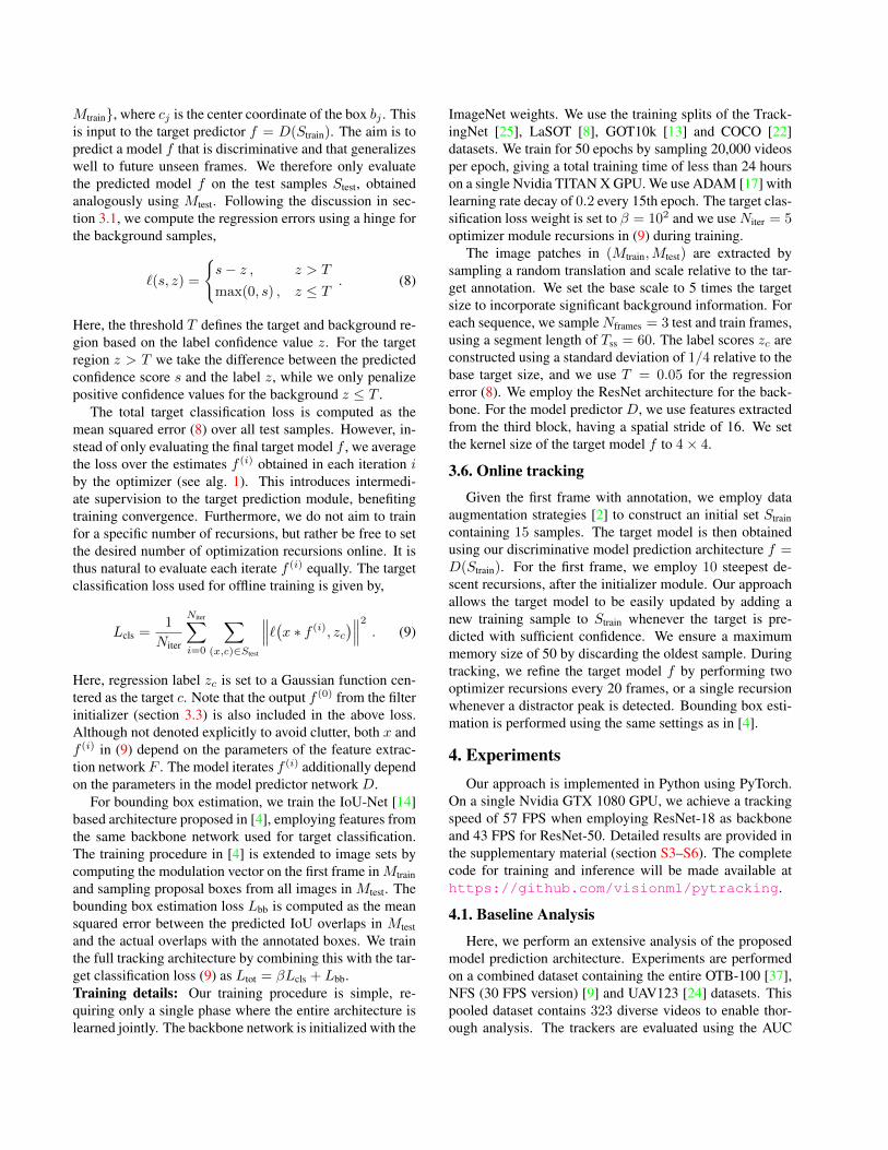
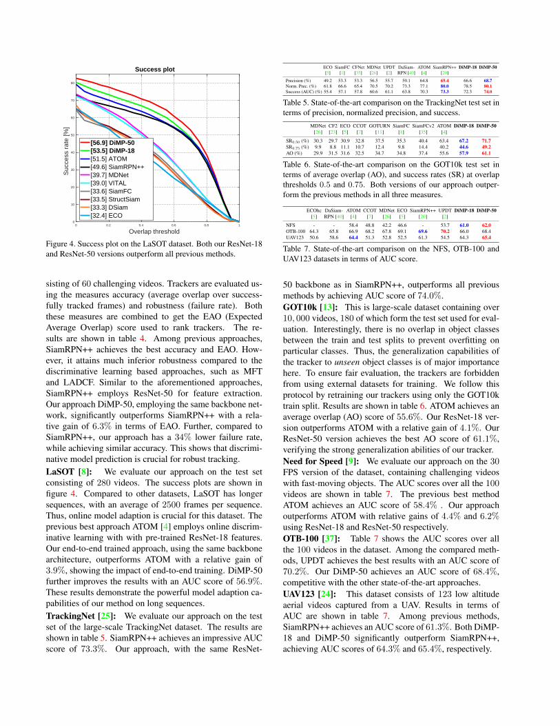
Figure 4. Success plot on the LaSOT dataset. Both our ResNet-18and ResNet-50 versions outperform all previous methods.

sisting of 60 challenging videos. Trackers are evaluated us-ing the measures accuracy (average overlap over success-fully tracked frames) and robustness (failure rate). Boththese measures are combined to get the EAO (ExpectedAverage Overlap) score used to rank trackers. The re-sults are shown in table 4. Among previous approaches,SiamRPN++ achieves the best accuracy and EAO. How-ever, it attains much inferior robustness compared to thediscriminative learning based approaches, such as MFTand LADCF. Similar to the aforementioned approaches,SiamRPN++ employs ResNet-50 for feature extraction.Our approach DiMP-50, employing the same backbone net-work, significantly outperforms SiamRPN++ with a rela-tive gain of 6.3% in terms of EAO. Further, compared toSiamRPN++, our approach has a 34% lower failure rate,while achieving similar accuracy. This shows that discrimi-native model prediction is crucial for robust tracking.LaSOT [8]: We evaluate our approach on the test setconsisting of 280 videos. The success plots are shown infigure 4. Compared to other datasets, LaSOT has longersequences, with an average of 2500 frames per sequence.Thus, online model adaption is crucial for this dataset. Theprevious best approach ATOM [4] employs online discrim-inative learning with with pre-trained ResNet-18 features.Our end-to-end trained approach, using the same backbonearchitecture, outperforms ATOM with a relative gain of3.9%, showing the impact of end-to-end training. DiMP-50further improves the results with an AUC score of 56.9%.These results demonstrate the powerful model adaption ca-pabilities of our method on long sequences.TrackingNet [25]: We evaluate our approach on the testset of the large-scale TrackingNet dataset. The results areshown in table 5. SiamRPN++ achieves an impressive AUCscore of 73.3%. Our approach, with the same ResNet-

ECO SiamFC CFNet MDNet UPDT DaSiam- ATOM SiamRPN++ DiMP-18 DiMP-50[5] [1] [35] [26] [2] RPN [40] [4] [20]

Precision (%) 49.2 53.3 53.3 56.5 55.7 59.1 64.8 69.4 66.6 68.7Norm. Prec. (%) 61.8 66.6 65.4 70.5 70.2 73.3 77.1 80.0 78.5 80.1Success (AUC) (%) 55.4 57.1 57.8 60.6 61.1 63.8 70.3 73.3 72.3 74.0

Table 5. State-of-the-art comparison on the TrackingNet test set interms of precision, normalized precision, and success.

MDNet CF2 ECO CCOT GOTURN SiamFC SiamFCv2 ATOM DiMP-18 DiMP-50[26] [23] [5] [7] [11] [1] [35] [4]

SR0.50 (%) 30.3 29.7 30.9 32.8 37.5 35.3 40.4 63.4 67.2 71.7SR0.75 (%) 9.9 8.8 11.1 10.7 12.4 9.8 14.4 40.2 44.6 49.2AO (%) 29.9 31.5 31.6 32.5 34.7 34.8 37.4 55.6 57.9 61.1

Table 6. State-of-the-art comparison on the GOT10k test set interms of average overlap (AO), and success rates (SR) at overlapthresholds 0.5 and 0.75. Both versions of our approach outper-form the previous methods in all three measures.

ECOhc DaSiam- ATOM CCOT MDNet ECO SiamRPN++ UPDT DiMP-18 DiMP-50[5] RPN [40] [4] [7] [26] [5] [20] [2]

NFS - - 58.4 48.8 42.2 46.6 - 53.7 61.0 62.0OTB-100 64.3 65.8 66.9 68.2 67.8 69.1 69.6 70.2 66.0 68.4UAV123 50.6 58.6 64.4 51.3 52.8 52.5 61.3 54.5 64.3 65.4

Table 7. State-of-the-art comparison on the NFS, OTB-100 andUAV123 datasets in terms of AUC score.

50 backbone as in SiamRPN++, outperforms all previousmethods by achieving AUC score of 74.0%.GOT10k [13]: This is large-scale dataset containing over10, 000 videos, 180 of which form the test set used for eval-uation. Interestingly, there is no overlap in object classesbetween the train and test splits to prevent overfitting onparticular classes. Thus, the generalization capabilities ofthe tracker to unseen object classes is of major importancehere. To ensure fair evaluation, the trackers are forbiddenfrom using external datasets for training. We follow thisprotocol by retraining our trackers using only the GOT10ktrain split. Results are shown in table 6. ATOM achieves anaverage overlap (AO) score of 55.6%. Our ResNet-18 ver-sion outperforms ATOM with a relative gain of 4.1%. OurResNet-50 version achieves the best AO score of 61.1%,verifying the strong generalization abilities of our tracker.Need for Speed [9]: We evaluate our approach on the 30FPS version of the dataset, containing challenging videoswith fast-moving objects. The AUC scores over all the 100videos are shown in table 7. The previous best methodATOM achieves an AUC score of 58.4% . Our approachoutperforms ATOM with relative gains of 4.4% and 6.2%using ResNet-18 and ResNet-50 respectively.OTB-100 [37]: Table 7 shows the AUC scores over allthe 100 videos in the dataset. Among the compared meth-ods, UPDT achieves the best results with an AUC score of70.2%. Our DiMP-50 achieves an AUC score of 68.4%,competitive with the other state-of-the-art approaches.UAV123 [24]: This dataset consists of 123 low altitudeaerial videos captured from a UAV. Results in terms ofAUC are shown in table 7. Among previous methods,SiamRPN++ achieves an AUC score of 61.3%. Both DiMP-18 and DiMP-50 significantly outperform SiamRPN++,achieving AUC scores of 64.3% and 65.4%, respectively.

5. ConclusionsWe propose a discriminative tracking approach that is

trained offline in an end-to-end manner. Our approach isderived from a discriminative learning loss by applying aniterative optimization procedure. By employing a steepestdescent based optimizer and an effective model initializer,our approach can predict a powerful discriminative model inonly a few optimization steps. Further, our approach learnsthe discriminative loss during offline training by minimiz-ing the prediction error on unseen test frames. Our approachsets a new state-of-the-art on 6 tracking benchmarks, whileoperating at over 40 FPS.

References[1] L. Bertinetto, J. Valmadre, J. F. Henriques, A. Vedaldi, and

P. H. Torr. Fully-convolutional siamese networks for objecttracking. In ECCV workshop, 2016. 1, 2, 8

[2] G. Bhat, J. Johnander, M. Danelljan, F. S. Khan, and M. Fels-berg. Unveiling the power of deep tracking. In ECCV, 2018.6, 7, 8

[3] D. S. Bolme, J. R. Beveridge, B. A. Draper, and Y. M. Lui.Visual object tracking using adaptive correlation filters. InCVPR, 2010. 3

[4] M. Danelljan, G. Bhat, F. S. Khan, and M. Felsberg. ATOM:Accurate tracking by overlap maximization. In CVPR, 2019.2, 3, 6, 7, 8, 12

[5] M. Danelljan, G. Bhat, F. Shahbaz Khan, and M. Felsberg.ECO: efficient convolution operators for tracking. In CVPR,2017. 2, 3, 8

[6] M. Danelljan, G. Hager, F. Shahbaz Khan, and M. Felsberg.Learning spatially regularized correlation filters for visualtracking. In ICCV, 2015. 2

[7] M. Danelljan, A. Robinson, F. Khan, and M. Felsberg. Be-yond correlation filters: Learning continuous convolutionoperators for visual tracking. In ECCV, 2016. 2, 8

[8] H. Fan, L. Lin, F. Yang, P. Chu, G. Deng, S. Yu, H. Bai,Y. Xu, C. Liao, and H. Ling. Lasot: A high-qualitybenchmark for large-scale single object tracking. CoRR,abs/1809.07845, 2018. 2, 6, 8, 12

[9] H. K. Galoogahi, A. Fagg, C. Huang, D. Ramanan, andS. Lucey. Need for speed: A benchmark for higher framerate object tracking. In ICCV, 2017. 2, 6, 8, 12

[10] Q. Guo, W. Feng, C. Zhou, R. Huang, L. Wan, and S. Wang.Learning dynamic siamese network for visual object track-ing. In ICCV, 2017. 2

[11] D. Held, S. Thrun, and S. Savarese. Learning to track at 100fps with deep regression networks. In ECCV, 2016. 8

[12] J. F. Henriques, R. Caseiro, P. Martins, and J. Batista. High-speed tracking with kernelized correlation filters. TPAMI,37(3):583–596, 2015. 2, 3, 7

[13] L. Huang, X. Zhao, and K. Huang. Got-10k: A large high-diversity benchmark for generic object tracking in the wild.arXiv preprint arXiv:1810.11981, 2018. 2, 6, 8

[14] B. Jiang, R. Luo, J. Mao, T. Xiao, and Y. Jiang. Acquisitionof localization confidence for accurate object detection. InECCV, 2018. 5, 6

[15] I. Jung, J. Son, M. Baek, and B. Han. Real-time mdnet. InECCV, 2018. 13

[16] H. Kiani Galoogahi, A. Fagg, and S. Lucey. Learningbackground-aware correlation filters for visual tracking. InICCV, 2017. 2, 7

[17] D. P. Kingma and J. Ba. Adam: A method for stochasticoptimization. In ICLR, 2014. 6

[18] M. Kristan, A. Leonardis, J. Matas, M. Felsberg,R. Pfugfelder, L. C. Zajc, T. Vojir, G. Bhat, A. Lukezic,A. Eldesokey, G. Fernandez, and et al. The sixth visual ob-ject tracking vot2018 challenge results. In ECCV workshop,2018. 2, 7, 12

[19] M. Kristan, J. Matas, A. Leonardis, M. Felsberg, L. Cehovin,G. Fernandez, T. Vojır, G. Nebehay, R. Pflugfelder, andG. Hger. The visual object tracking vot2015 challenge re-sults. In ICCV workshop, 2015. 12

[20] B. Li, W. Wu, Q. Wang, F. Zhang, J. Xing, and J. Yan.Siamrpn++: Evolution of siamese visual tracking with verydeep networks. In CVPR, 2019. 7, 8, 12, 13

[21] B. Li, J. Yan, W. Wu, Z. Zhu, and X. Hu. High performancevisual tracking with siamese region proposal network. InCVPR, 2018. 1, 2, 3

[22] T. Lin, M. Maire, S. J. Belongie, L. D. Bourdev, R. B. Gir-shick, J. Hays, P. Perona, D. Ramanan, P. Dollar, and C. L.Zitnick. Microsoft COCO: common objects in context. InECCV, 2014. 6, 12

[23] C. Ma, J.-B. Huang, X. Yang, and M.-H. Yang. Hierarchicalconvolutional features for visual tracking. In ICCV, 2015. 2,8

[24] M. Mueller, N. Smith, and B. Ghanem. A benchmark andsimulator for uav tracking. In ECCV, 2016. 2, 6, 8, 12

[25] M. Muller, A. Bibi, S. Giancola, S. Al-Subaihi, andB. Ghanem. Trackingnet: A large-scale dataset and bench-mark for object tracking in the wild. In ECCV, 2018. 2, 6, 8,12

[26] H. Nam and B. Han. Learning multi-domain convolutionalneural networks for visual tracking. In CVPR, 2016. 2, 8

[27] J. Nocedal and S. J. Wright. Numerical Optimization.Springer, 2nd edition, 2006. 4

[28] E. Park and A. C. Berg. Meta-tracker: Fast and robust onlineadaptation for visual object trackers. In ECCV, 2018. 2

[29] E. Real, J. Shlens, S. Mazzocchi, X. Pan, and V. Vanhoucke.Youtube-boundingboxes: A large high-precision human-annotated data set for object detection in video. CVPR, 2017.12

[30] S. Ren, K. He, R. B. Girshick, and J. Sun. Faster R-CNN:towards real-time object detection with region proposal net-works. In NIPS, 2015. 2

[31] O. Russakovsky, J. Deng, H. Su, J. Krause, S. Satheesh,S. Ma, Z. Huang, A. Karpathy, A. Khosla, M. Bernstein,A. C. Berg, and L. Fei-Fei. ImageNet Large Scale VisualRecognition Challenge. IJCV, pages 1–42, April 2015. 12,13

[32] J. R. Shewchuk. An introduction to the conjugate gradientmethod without the agonizing pain. Technical report, Pitts-burgh, PA, USA, 1994. 4

[33] C. Sun, D. Wang, H. Lu, and M. Yang. Correlation trackingvia joint discrimination and reliability learning. In CVPR,2018. 7

[34] R. Tao, E. Gavves, and A. W. M. Smeulders. Siamese in-stance search for tracking. In CVPR, 2016. 1, 2

[35] J. Valmadre, L. Bertinetto, J. F. Henriques, A. Vedaldi, andP. H. S. Torr. End-to-end representation learning for correla-tion filter based tracking. In CVPR, 2017. 2, 7, 8

[36] Q. Wang, Z. Teng, J. Xing, J. Gao, W. Hu, and S. J. Maybank.Learning attentions: Residual attentional siamese networkfor high performance online visual tracking. In CVPR, 2018.2

[37] Y. Wu, J. Lim, and M.-H. Yang. Object tracking benchmark.TPAMI, 37(9):1834–1848, 2015. 2, 6, 7, 8, 12

[38] T. Xu, Z. Feng, X. Wu, and J. Kittler. Learning adaptive dis-criminative correlation filters via temporal consistency pre-serving spatial feature selection for robust visual tracking.CoRR, abs/1807.11348, 2018. 7

[39] Y. Yao, X. Wu, S. Shan, and W. Zuo. Joint representationand truncated inference learning for correlation filter basedtracking. In ECCV, 2018. 2

[40] Z. Zhu, Q. Wang, L. Bo, W. Wu, J. Yan, and W. Hu.Distractor-aware siamese networks for visual object track-ing. In ECCV, 2018. 2, 7, 8

Supplementary Material

This supplementary material provides additional detailsand results. Section S1 derives the closed form expressionof the filter gradient, employed in the optimizer module. Insection S2 we derive the application of the Jacobian in or-der to compute the quantity h, employed in algorithm 1 inthe paper. In section S3 we provide detailed results on theVOT2018 dataset, while in section S4, we provide detailedresults on the LaSOT dataset. We also provide additionaldetails on the NFS, OTB100 and UAV123 datasets in sec-tion S5. Finally, we analyze the impact when training withless data in section S6.

S1. Closed-Form Expression for∇LHere, we derive a closed-form expression for the gradi-

ent of the loss (1) in the main paper, also restated here,

L(f) =1

|Strain|∑

(x,c)∈Strain

‖r(s, c)‖2 + ‖λf‖2 . (S1)

Here, s = x ∗ f is the score map obtained after convolvingthe deep feature map xwith the target model f . The trainingset is given by Strain = {(xj , cj)}nj=1. The residual functionr(s, c) is defined as (also eq. (2) in the paper),

r(s, c) = vc · (mcs+ (1−mc) max(0, s)− yc) . (S2)

The gradient ∇L(f) of the loss (S1) w.r.t. the filter coeffi-cients f is then computed as,

∇L(f) =2

|Strain|∑

(x,c)∈Strain

(∂rs,c∂f

)T

rs,c + 2λ2f . (S3)

Here, we have defined rs,c = r(s, c) and ∂rs,c∂f corresponds

to the Jacobian of the residual function (S2) w.r.t. the filtercoefficients f . Using eq. (S2) we obtain,

∂rs,c∂f

= diag(vcmc)∂s

∂f+ diag ((1−mc) · 1s>0)

∂s

∂f

= diag(qc)∂s

∂f. (S4)

Here, diag(qc) denotes a diagonal matrix containing the el-ements in qc. Further, qc = vcmc + (1 − mc) · 1s>0 iscomputed using only point-wise operations, where 1s>0 is1 for positive s and 0 otherwise. Using eqs. (S3) and (S4)we finally obtain,

∇L(f) =2

|Strain|∑

(x,c)∈Strain

(∂s

∂f

)T

(qc · rs,c) + 2λ2f .

(S5)Here, · denotes the element-wise product. The multipli-cation with the transposed Jacobian

(∂s∂f

)Tcorresponds to

backpropagation of the input qc · rs,c through the convo-lution layer f 7→ x ∗ f . This is implemented as a trans-posed convolution with x. The closed-form expression (S5)is thus easily implemented using standard operations in adeep learning library like PyTorch.

S2. Calculation of h in Algorithm 1

In this section, we show the calculation of h =J (i)∇L(f (i)), used when determining the optimal steplength α in Algorithm 1 in the main paper. Since weonly need the squared L2 norm of h in step length calcu-lation, we will directly derive an expression for ‖h‖2 =

‖J (i)∇L(f (i))‖2. Here, J (i) = ∂ξ∂f

∣∣∣f(i)

is the Jacobian

of the residual vector ξ of loss (S1), evaluated at the filterestimate f (i). Not to be confused with the residual func-tion (S2), the residual vector ξ is obtained as the concate-nation of individual residuals ξj = r(xj ∗ f, cj)/

√n for

j ∈ {1, . . . , n} and ξj = λf for j = n + 1. Here,n = |Strain| is the number of samples in Strain. Consequently,we get,

‖h‖2 =∥∥∥J (i)∇L(f (i))

∥∥∥2

(S6)

=

n+1∑j=1

∥∥∥∥∥ ∂ξj∂f∣∣∣∣f(i)

∇L(f (i))

∥∥∥∥∥2

=

n∑j=1

∥∥∥∥∥ 1√n

∂r(xj ∗ f, cj)∂f

∣∣∣∣f(i)

∇L(f (i))

∥∥∥∥∥2

+∥∥∥λ∇L(f (i))

∥∥∥2

=1

n

∑(x,c)∈Strain

∥∥∥∥∥ ∂rs,c∂f

∣∣∣∣f(i)

∇L(f (i))

∥∥∥∥∥2

+∥∥∥λ∇L(f (i))

∥∥∥2

.

Using eqs. (S6) and (S4) we finally obtain,

‖h‖2 =1

|Strain|∑

(x,c)∈Strain

∥∥∥∥∥qc ·(∂s

∂f

∣∣∣∣f(i)

∇L(f (i))

)∥∥∥∥∥2

+

‖λ∇L(f (i))‖2

=1

|Strain|∑

(x,c)∈Strain

∥∥∥qc · (x ∗ ∇L(f (i)))∥∥∥2

+

‖λ∇L(f (i))‖2

As described in section S1,∇L(f (i)) is computed using theclosed-form expression (S5). The term ∂s

∂f

∣∣∣f(i)∇L(f (i))

corresponds to convolution of x with ∇L(f (i)), i.e.∂s∂f

∣∣∣f(i)∇L(f (i)) = x ∗ ∇L(f (i)). Thus, ‖h‖2 is com-

puted easily using standard operations from deep learninglibraries.

50 100 200 500 1000

Sequence length

0

0.1

0.2

0.3

0.4

0.5

0.6

Exp

ecte

d o

ve

rla

p

DiMP-50 [0.440]SiamRPN++ [0.415]

DiMP-18 [0.402]

ATOM [0.401]

LADCF [0.389]

MFT [0.385]

DaSiamRPN [0.383]

UPDT [0.378]

RCO [0.376]

DRT [0.356]

Figure S1. Expected average overlap curve on the VOT2018dataset, showing the expected overlap between tracker predictionand ground truth for different sequence lengths. The EAO mea-sure, computed as the average of the expected average overlap overtypical sequence lengths (grey region in the plot), is shown in thelegend. Our approach achieves the best EAO score, outperformingthe previous best approach SiamRPN++ [20] with a relative gainof 6.3% in terms of EAO.

S3. Detailed Results on VOT2018

In this section, we provide detailed results on theVOT2018 [18] dataset. The VOT protocol evaluates theexpected average overlap (EAO) between the tracker pre-dictions and the ground truth bounding boxes for differentsequence lengths. The trackers are then ranked using theEAO measure, which computes the average of the expectedaverage overlaps over typical sequence lengths. We referto [19] for further details about the EAO computation. Fig-ure S1 plots the expected average overlap for different se-quence lengths on VOT2018 dataset. Our approach DiMP-50 achieves the best EAO score of 0.44.

S4. Detailed Results on LaSOT

Here, we provide the normalized precision plots on theLaSOT [8] dataset. These are obtained in the followingmanner. First, the normalized precision score Pnorm is com-puted as the percentage of frames in which the distancebetween the target location predicted by the tracker andthe ground truth, relative to the target size, is less than acertain threshold. The normalized precision score over allthe the videos are then plotted over a range of thresholds[0, 0.5] to obtain the normalized precision plots. The track-ers are ranked using the area under the resulting curve. Fig-ure S2 shows the normalized precision plots over all 280videos in the LaSOT dataset. Both our ResNet-18 (DiMP-18) and ResNet-50 (DiMP-50) versions outperform all pre-vious methods, achieving relative gains of 5.9% and 12.8%

0 0.05 0.1 0.15 0.2 0.25 0.3 0.35 0.4 0.45 0.5

Location error threshold

0

0.1

0.2

0.3

0.4

0.5

0.6

0.7

0.8

Pre

cisi

on

Normalized Precision plots of OPE on LaSOT Testing Set

[0.643] ETCOM50[0.610] ETCOM18[0.576] ATOM[0.569] SiamRPN++[0.460] MDNet[0.453] VITAL[0.420] SiamFC[0.418] StructSiam[0.405] DSiam[0.338] ECO

Figure S2. Normalized precision plot on the LaSOT dataset. Bothour ResNet-18 and ResNet-50 versions outperform all previousmethods by significant margins.

over the previous best method, ATOM [4].

S5. Detailed Results on NFS, OTB-100, andUAV123

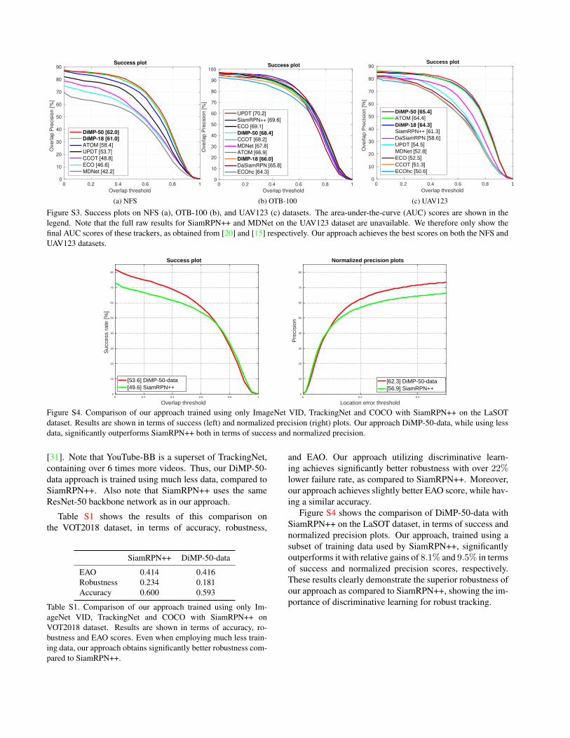
Here, we provide detailed results on NFS [9], OTB-100[37], and UAV123 [24] datasets. We use the overlap preci-sion (OP) metric for evaluating the trackers. The OP scoredenotes the percentage of frames in a video for which theintersection-over-union (IoU) overlap between the trackerprediction and the ground truth bounding box exceeds a cer-tain threshold. The mean OP score over all the videos in adataset are plotted over a range of thresholds [0, 1] to obtainthe success plot. The area under this plot provides the AUCscore, which is used to rank the trackers. We refer to [37]for further details. The success plots over the entire NFS,OTB-100, and UAV123 datasets are shown in figure S3.Our tracker using ResNet-50 backbone, denoted DiMP-50,achieves the best results on both NFS and UAV123 datasets,while obtaining results competitive with the state-of-the-arton the, now saturated, OTB-100 dataset. On the challeng-ing NFS dataset, our approach achieves an absolute gain of3.6% AUC score over the previous best method ATOM [4].

S6. Impact of Training DataHere, we investigate the impact of training our approach

with less tracking data. We train a version of our trackerwith the ResNet-50 backbone using only the ImageNet VID[31], TrackingNet [25] and COCO [22] datasets. We com-pare this version, denoted DiMP-50-data with the state-of-the-art Siamese tracker, SiamRPN++ [20], trained using Im-ageNet VID, YouTube-BB [29], COCO and ImageNet DET

0 0.2 0.4 0.6 0.8 1

Overlap threshold

0

10

20

30

40

50

60

70

80

90

Overlap P

recis

ion [%

]

Success plot

DiMP-50 [62.0]

DiMP-18 [61.0]

ATOM [58.4]

UPDT [53.7]

CCOT [48.8]

ECO [46.6]

MDNet [42.2]

(a) NFS

0 0.2 0.4 0.6 0.8 1

Overlap threshold

0

10

20

30

40

50

60

70

80

90

100

Ove

rla

p P

recis

ion

[%

]

Success plot

UPDT [70.2]

SiamRPN++ [69.6]

ECO [69.1]

DiMP-50 [68.4]

CCOT [68.2]

MDNet [67.8]

ATOM [66.9]

DiMP-18 [66.0]

DaSiamRPN [65.8]

ECOhc [64.3]

(b) OTB-100

0 0.2 0.4 0.6 0.8 1Overlap threshold

0

10

20

30

40

50

60

70

80

90

Ove

rlap

Pre

cisi

on [%

]

Success plot

DiMP-50 [65.4]ATOM [64.4]DiMP-18 [64.3]SiamRPN++ [61.3]DaSiamRPN [58.6]UPDT [54.5]MDNet [52.8]ECO [52.5]CCOT [51.3]ECOhc [50.6]

(c) UAV123

Figure S3. Success plots on NFS (a), OTB-100 (b), and UAV123 (c) datasets. The area-under-the-curve (AUC) scores are shown in thelegend. Note that the full raw results for SiamRPN++ and MDNet on the UAV123 dataset are unavailable. We therefore only show thefinal AUC scores of these trackers, as obtained from [20] and [15] respectively. Our approach achieves the best scores on both the NFS andUAV123 datasets.

0 0.2 0.4 0.6 0.8 1

Overlap threshold

0

10

20

30

40

50

60

70

80

Suc

cess

rat

e [%

]

Success plot

[53.6] DiMP-50-data[49.6] SiamRPN++

0 0.2 0.4

Location error threshold

0

10

20

30

40

50

60

70

80

Pre

cisi

on

Normalized precision plots

[62.3] DiMP-50-data[56.9] SiamRPN++

Figure S4. Comparison of our approach trained using only ImageNet VID, TrackingNet and COCO with SiamRPN++ on the LaSOTdataset. Results are shown in terms of success (left) and normalized precision (right) plots. Our approach DiMP-50-data, while using lessdata, significantly outperforms SiamRPN++ both in terms of success and normalized precision.

[31]. Note that YouTube-BB is a superset of TrackingNet,containing over 6 times more videos. Thus, our DiMP-50-data approach is trained using much less data, compared toSiamRPN++. Also note that SiamRPN++ uses the sameResNet-50 backbone network as in our approach.

Table S1 shows the results of this comparison onthe VOT2018 dataset, in terms of accuracy, robustness,

SiamRPN++ DiMP-50-data

EAO 0.414 0.416Robustness 0.234 0.181Accuracy 0.600 0.593

Table S1. Comparison of our approach trained using only Im-ageNet VID, TrackingNet and COCO with SiamRPN++ onVOT2018 dataset. Results are shown in terms of accuracy, ro-bustness and EAO scores. Even when employing much less train-ing data, our approach obtains significantly better robustness com-pared to SiamRPN++.

and EAO. Our approach utilizing discriminative learn-ing achieves significantly better robustness with over 22%lower failure rate, as compared to SiamRPN++. Moreover,our approach achieves slightly better EAO score, while hav-ing a similar accuracy.

Figure S4 shows the comparison of DiMP-50-data withSiamRPN++ on the LaSOT dataset, in terms of success andnormalized precision plots. Our approach, trained using asubset of training data used by SiamRPN++, significantlyoutperforms it with relative gains of 8.1% and 9.5% in termsof success and normalized precision scores, respectively.These results clearly demonstrate the superior robustness ofour approach as compared to SiamRPN++, showing the im-portance of discriminative learning for robust tracking.