Do Business Groups Use Dividends to Fund

Investments?∗

Radhakrishnan Gopalan, Vikram Nanda, and Amit Seru

This Version: March, 2005

∗Acknowledgements: We thank Vladimir Atanasov, Arnoud Boot, Amy Dittmar, Mara Faccio,Robert Kennedy, Han Kim, Joel Slemrod and the seminar participants at the Korean 2005 CorporateGovernance Conference, Ross School of Business at the University of Michigan and the William DavidsonInstitute at the University of Michigan for helpful comments and suggestions. The authors acknowledgeMitsui Finance Center, Center for International Business Education and the William Davidson Insti-tute, all at the University of Michigan for financial support and for acquiring the Prowess data set. Theauthors are from Ross School of Business at the University of Michigan. E-mail: gopalanr@umich.edu,vnanda@umich.edu (corresponding author), aseru@umich.edu. All remaining errors are our responsi-bility. Contact Address: Ross School of Business, Finance Department, 701 Tappan Street, Ann Arbor,Michigan 48109, USA. Phone: 734.763.0105. Fax: 734.936.0274.

Do Business Groups Use Dividends to Fund

Investments?

Abstract

We argue that business group insiders in emerging markets can use dividends as a transparent way

of transferring cash across group firms. We formalize this intuition in a model, endogenizing the group

structure and draw predictions regarding the dividend policy and insider holding in group firms. Our

main predictions are: (i) Dividends of a group firm should be positively associated with investment and

external equity financing in other member firms in the group; (ii) Insider holding in group firms should

decrease with firm age; and (iii) Insider holding in the young firms in the group should be positively

related to dividend distribution from the older firms in the group. We find strong support for all our

predictions using firm level data from six emerging markets.

Do Business Groups Use Dividends to Fund

Investments?

1 Introduction

Emerging economies are characterized by weak legal systems and poor investor protec-

tion. A well documented consequence is that firms in emerging economies – many of

them organized as business groups – are subject to severe agency conflicts between in-

siders and outside equity holders (Bertrand et al. (2002); Faccio et al. (2001); Claessens

et al. (2002)). It may seem surprising, therefore, that many group firms in these

economies consistently pay significant amounts of dividends and have dispersed outside

equity. For instance, the median group firm in India pays about 27% of its EBDITA

(Earnings Before Depreciation, Interest, Taxes and Amortization) as dividends and has

52% shareholding with small outside investors.1 In this paper, we offer and test a theory

of dividends and outside equity for firms belonging to business groups. We argue that

business group firms can use dividend distributions as a transparent way of transferring

cash across group firms in response to investment opportunities. Transparency may be

a virtue in a system where tax and other government agencies may demand to know the

source of funds employed in significant future investments. The expectation of dividend

payout, in turn, sustains outside equity in these firms. Our theory also offers a potential

explanation for the prevalence of business groups in emerging economies.

A number of mechanisms that sustain dividends in the presence of agency conflicts

have been proposed. In a recent study of dividend policies around the world, La Porta

et al. (2000) show that the legal and regulatory regime in place enables outside share-

holders to extract dividends from firms. In environments where the legal regime does

not provide sufficient protection to small shareholders, firm reputation and the need

to access external financial markets in future, can force insiders to pay out dividends

(Gomes, (2000)). Ours is a complementary, non reputation based, explanation for the

presence of dividends in environments where agency conflicts are severe and the legal

1In contrast, in the US, the median Compustat firm pays no dividends while among dividend payingfirms in Compustat the median dividend to EBDITA is around 15%.

1

regime is weak. We argue that the insider’s need to show a transparent and legitimate

source of income, can force him to pay dividends.

We focus on business groups since it is the dominant organizational form in emerging

markets (Khanna and Yafeh (forthcoming)). A typical business group has a set of

independent firms controlled by a common group of insiders, consisting of a founding

family and its associates. The shareholding patterns of group firms are usually complex,

with the insider owning equity both directly and indirectly through cross holdings. For

our purpose we define the horizontal business group, HBG as one polar case, where the

insider has direct shareholding in all the firms belonging to the group and there are no

cross holdings. The cases with cross holdings are regarded as vertical business groups

V BGs.

We develop a model that formalizes our intuition in the case of the HBG structure

and delivers predictions regarding the dividend policy and the distribution of insider

holding in group firms. In the model, we consider an entrepreneur who has an initial

project and may get a second project at a later date. The entrepreneur is wealth con-

strained and raises outside equity to finance the projects. He can divert firm resources

for his private benefit at a proportional cost. When the entrepreneur gets the second

project, he chooses between promoting it in the existing firm (a conglomerate structure)

or in a separate firm (a HBG structure). We show that whenever the entrepreneur

chooses the HBG structure, he limits his diversion and pays dividends while if he un-

dertakes the second project in a conglomerate structure, he diverts resources and does

not pay any dividends. We also show that in our set up a V BG structure is equivalent

to a conglomerate structure.

We argue that whenever entrepreneurs need to transfer large sums of money across

independent firms to finance investments, they will have to do so in a transparent man-

ner. Employing transparent means ensures that the source of money used for investment

is known to the public and the regulators. This may be important in situations wherein

expenditure of large sums of money (in the form of investments) without known sources

can be made difficult by scrutiny from tax authorities, security market regulators and

common financiers. Therefore, in our setup, diverted resources without known sources

can only be used by insiders for their private benefits. Our assumption is in line with

ones used in most models of diversion (Desai, Dyck and Zingales (2004); Durnev and

2

Kim (forthcoming); Freidman et al. (2003)). In the conglomerate structure cash can

be easily transferred across projects since these are undertaken within the same firm.

On the other hand a HBG structure, with independent firms, forces the entrepreneur

to employ a transparent means of transferring cash from the first project to the second

project. Dividends serve as one such transparent means. Anticipating these dividend

payments, outside investors are willing, ex-ante, to finance the first project – making the

HBG structure viable. Ex-post, after the first project is taken, entrepreneurs employ

the HBG structure whenever the cost of paying dividends to outside investors in the

first project is less than the costs of diversion from both the projects. Since the costs

of diversion, increases in the size and profitability of the second project, entrepreneurs

choose the HBG structure and pay dividends whenever the second project is sufficiently

large.2

In our theoretical and empirical analysis we focus on the HBG structure for two main

reasons. First, dividends as a means of transferring resources across firms has an unique

role in the case of HBGs. This enables us to develop sharp testable predictions. Second,

we have detailed data on the identity of firms belonging to a particular business group

for India and five east-asian countries – Malaysia, Taiwan, Philippines, South Korea and

Thailand – where business groups predominantly have a HBG structure (Bertrand et

al. (2001); Claessens et al. (2000)). Although our analysis is focussed on HBGs from

these six countries, we feel our analysis may be applicable to a broader set of firms since

the data from earlier studies indicates that the extent of pyramiding and cross holding

may be fairly limited in the case of public group firms.3

The central crux of our theory is that insiders of business groups use dividends from

2The amount to be diverted increases with the size of the second project and since the cost ofdiversion are proportional, the costs increase with the size of the second project.

3A popular method employed in the literature for measuring the extent of pyramiding is to examinethe ratio of insider’s effective cash flow rights in a firm to his control rights in the firm. For the purposeof this ratio, control rights are measured as the minimum shareholding in the chain of control. Forexample, in a group with two layers of pyramiding and where the insider controls a subsidiary througha parent, if α1 is the insider’s direct shareholding in the parent and α2 the parent’s shareholding inthe subsidiary, the O/C ratio for the subsidiary is O/C = α1α2

min{α1,α2} . While this ratio is equal to 1for HBGs, this ratio is in general less than 1 for V BGs. Faccio et al. (2001) show that the medianO/C for a sample of Asian firms across 9 countries is 0.778. In the context of the earlier example, thisindicates that the maximum of either the insider’s holding in the parent or the parent’s holding in thesubsidiary should be 77.8%.

3

existing firms to finance their equity investments in the newer firms in the group. Our

first two predictions follow from this. Specifically, (1) Group firms will distribute more

dividends than stand alone firms and (2) Dividends of a group firm will be positively

associated with investments and increase in external equity in other firms in the group.

An important corollary that emerges from our model is that as groups become older,

insiders should have greater holding in subsequent firms in the group on account of

their greater wealth. Our last two predictions follow this rationale. Formally stated,

(3) Group firms will have greater insider holding than stand alone firms and (4) Insider

holding will decrease with firm age for group firms and insider holding in younger firms

in the group will be positively related to dividend payments from the older firms.

We conduct detailed tests of our predictions using a panel data of 1, 932 group firms

and 2, 850 stand-alone firms from India and 493 group firms from Malaysia, Taiwan,

Phillipines, South Korea and Thailand. Due to the large difference in sample size be-

tween India and East Asia, we run separate tests for the two samples. We collect

information on firm financials, group affiliation, industry affiliation and insider holding

for these firms. We are able to test all the predictions using the Indian sample, since

besides information on group firms, we have reliable information on stand-alone firms.

We test only predictions involving group firms on the East Asian sample.4 While a

number of our predictions are not easily obtained from a reputation based explanation

of dividend policy, some of our predictions are consistent with a reputation model. Since

it is likely that reputation concerns are likely not to vary with time, we use firm fixed

effects in our tests and demonstrate that our empirical results are more consistent with

our theory.

Our empirical results strongly support all our predictions. In particular, we find that

for Indian business groups 14% of the insider’s equity investment in member firms is

financed by his share of (one year’s) dividends from his group firms. (The corresponding

number is 8% for the sample of East Asian firms). We also find that group insider

holding is 10% greater in a firm which is 10 years younger than the oldest firm in the

group. (The corresponding number is 8% for the sample of East Asian firms). These

results suggest that group insiders do use dividends to fund part of their investment in

other firms in the group and as groups get older, insiders accumulate wealth and use it to

4We are unable to test predictions involving stand alone and group firms in the East-Asian sampledue to data constraints. We will explain this issue in detail in the data section

4

acquire greater fraction of equity in the newer firms in the group. Our results are robust

to alternate explanations (e.g., tunnelling), model specifications (e.g., first differences

estimation instead of a fixed effects), variable definitions and sub-period analysis.

The rest of the paper is organized as follows: In Section 2, we present a survey of

the literature relevant to our topic. In Section 3, we present our model while Section 4

formalizes our main predictions and discusses our data. In Section 5, we describe our

empirical methodology and provide our results. Section 6 presents robustness of our

results and we conclude in Section 7. All proofs are in the Appendix.

2 Related Literature

Our paper is related to two strands of literature – the one on agency theories of dividends

and the other on business groups in emerging economies. The theoretical literature on

agency theories of dividends is vast (Easterbrook (1984); Jensen (1986); Fluck (1998;

1999); Hart and Moore (1994); Myers (2000); Gomes (2000) and Zwiebel (1996)). The

main idea of these papers is that cash inside the firm can be wasted by insiders in

unproductive investments and for their private benefit. Dividends reduce surplus cash

inside the firm and hence are optimal. The paper in the same spirit as ours is Fluck

(1998), which justifies the presence of outside equity in an environment where managers

can use firm cash for their private benefit. In Fluck (1998), outside equity holders have

control rights over firm assets and can threaten to remove the manager. Every period the

manager pays the minimum dividend required to prevent removal. The main difference

between this model and ours is that we assume full control rights with firm insiders.

This assumption is justified in the context of an emerging market, where laws are not

effectively implemented, asset markets are illiquid (Shleifer and Vishny (1992)) and the

market for corporate control is non-existent. Hence in contrast to Fluck, in our model

it is essential that dividends be optimal from the point of view of the insider.

Our paper adds to the prior empirical work testing the agency theory of dividends. In

a influential study of dividend policies of firms around the world, La Porta et al. (2000)

contrast a reputation based theory of dividends, where firm insiders pay dividends to

retain the ability to access the financial markets in future with one based on the legal

regime empowering outside shareholders to extract dividends from insiders. They find

5

significant support for the legal regime based theory. Our paper offers a complementary

explanation for the presence of dividends in environments, where the legal regime does

not provide sufficient protection to minority shareholders. In another paper on firm

dividend policies, Faccio et al. (2001) contrast the dividend policies of firms belonging

to V BGs in East Asia and Western Europe and establish a relationship between dividend

policies and the amount of pyramiding (O/C ratio). In contrast to Faccio et al. (2001),

we endogenize the group structure and explore the rationale for insiders to pay dividends

in firms belonging to HBGs. Furthermore, our analysis also extends to explaining the

distribution of insider holding in group firms.

The other strand of literature that our work relates to is on business groups. The

broader business group literature has investigated the financial and managerial inter-

linkages between the firms of business groups. Some papers identify risk sharing as

a significant benefit of the financial linkages among group firms. In a comprehensive

study of business groups in 15 countries, Khanna and Yafeh (forthcoming) document

that Indian business groups engage in liquidity smoothing. Another benefit of financial

interlinkages claimed in literature is in overcoming credit rationing problems. With a

larger reputation capital at stake, business groups refrain from reneging on contracts

with lenders and thus enable extension of credit (See Kali (2002)). In a recent study

of Indian business groups, Van der Molen and Gangopadhyay (2003) show that firms

belonging to groups have lower cash flow sensitivity of investment than stand alone

firms. They interpret this evidence as indicating lower financial constraints for business

group firms. On the negative side it has been argued that the financial linkages among

group firms results in agency conflicts between the insiders and minority shareholders.

According to Claessens et al. (2002), groups are associated with minority shareholder

expropriation in Asia. Freidman et al. (2003) as well as Bertrand et al. (2002) similarly

view groups as institutions that are associated with poor protection of property rights

enabling ‘tunnelling’ of funds from minority shareholders to the group insiders. Thus,

risk sharing/overcoming credit constraints on the one hand, and tunnelling on the other,

provide the two contrasting images of intra-group behavior.

One drawback of the literature on business groups discussed above is that, unlike

our approach, it takes the group structure as a given and explores the benefits and costs

of the structure. One exception is a recent paper by Almeida and Wolfenzon (2004)

on pyramidal ownership groups. Almeida and Wolfenzon argue that pyramidal groups

6

enable insiders to use all the retained earnings of the group firm for future investments

and should be important in situations where financial markets are not well developed

and private benefits are more important. Similar to their paper, we also offer a reason

for the presence of business group structure in emerging markets. However, our paper

differs from theirs on a number of dimensions. Firstly, we are primarily concerned with

HBGs while they offer a theory of V BGs. Secondly, while our main focus is to explain

dividend policies among group firms, their focus is on endogenizing the V BG structure.

Finally, whereas we offer a potential rationale for the presence of independent firms

in business groups, they do not offer any explanation for why a group is set up with

separate independent firms.

3 Model

In this section we illustrate how a horizontal business group structure (HBG) with div-

idend payout can arise endogenously – even when insiders can divert resources. The

model allows us to develop testable predictions about the dividend policies of firms

belonging to HBGs. We start by describing the agents, project and the contract possi-

bilities.

3.1 Agents, Project and Contract Possibilities

Consider an economy with an entrepreneur, atomistic investors and lenders. All agents

are risk neutral and the risk free interest rate is 0. There are three dates 0, 1 and

2 and two periods. There is no asymmetric information in the model. At date 0 the

entrepreneur gets his initial project (the A project). He is wealth constrained (his wealth

consists of the project) and requires external financing to undertake the project. The

project entails an investment of Ia at date 0 and will produce a payoff of Xa at date

1. The project has a positive net present value i.e., Xa > Ia. It is common knowledge

that the entrepreneur can also get a second project (the B project). The entrepreneur

gets the B project with probability p. This project requires an investment of Ib at date

1 and results in a cash flow of Xb at date 2. The B project also has a positive NPV,

i.e., Xb > Ib. Since both projects have positive NPV, in a first best world, both projects

7

would be implemented.

Given our focus on dividend policies and outside equity, we simplify the analysis by

assuming that the entrepreneur raises external capital by selling equity. In the Hart and

Moore (1994) incomplete contract setting, the absence of debt financing is consistent

with a zero liquidation value for the projects, which we assume to be the case for the A

and B projects. Our conclusions and intuition are, however, unaffected if the projects

are partly funded by debt, though the analysis is more involved. The entrepreneur or

insider sells equity to dispersed rational investors – though de facto he retains full control

rights over the projects.5 This is not an unreasonable assumption in the case of emerging

markets where the controlling insiders do not face any takeover threat and can usurp

the control rights through a number of means like friendly institutional investors and by

filling the board of directors with insiders and friends and family (Burkart, Panunzi and

Shleifer (2003)).

We make some important assumptions about the legal and regulatory environment.

The first assumption is that project cash flows, though observable, are not verifiable and

hence cannot be contracted upon. The second assumption is that insiders can divert cash

from the firms to their private benefit at a cost, however, their ability to do so is limited

in two (relatively mild) ways. The first limit we impose on insider diversion is that

shareholder distributions like dividend payments are verifiable and contractible. Hence,

the insider cannot pay preferential dividends to himself. The second constraint on the

diversion is that the regulatory environment includes monitoring by public authorities

(e.g., tax collectors), part of whose responsibility is to detect undeclared income. Due to

the second constraint, insiders cannot immediately publicly consume or reinvest diverted

funds without detection (while in the authority’s jurisdiction). The diverted resources

are, however, available to the insider for private consumption later – say by, squirreling

the money away to locations such as the notorious “Secret Swiss Bank Accounts” for a

period of time. As a consequence, if a firm requires cash, either for investment or for debt

repayment, an insider cannot divert the cash from another firm and use it to finance the

first firm’s requirements without detection. He will have to use some legitimate means

to transfer cash. We study the role played by dividends in facilitating such transfer.

It is worth noting that, in most models of diversion it is implicitly assumed that

5From now on, depending on context we will use the terms entrepreneur and insider interchangeably.

8

diverted resources are used for private benefit (Desai, Dyck and Zingales (2004); Durnev

and Kim (forthcoming); Freidman et al. (2003)). In these models either diversion is

explicitly modelled as occurring from the final cash flows or as being used for private

benefits. In either case, diversion is not used to fund any public expenditure.

3.2 Managerial Diversion

At some cost the insider can divert the cash flows of the project to his private ben-

efit. For simplicity we assume a proportional or linear cost of diversion. That is, the

insider gets $β < 1 for every $1 diverted. Hence, 1− β represents the cost of diversion.

In economies with lax regulations, where diversion is easier, β will be high, whereas

economies with tighter regulations will have a low β.

Our assumption of proportional diversion costs is different from other models of

diversion that assume a convex cost of diversion (Desai, Dyck and Zingales (2004);

Durnev and Kim (forthcoming); Freidman et al. (2003)). With convex diversion costs,

assumptions about the cost function tends to determine the amount diverted and, hence,

the residual that is paid out as a dividend. To obtain interesting, testable predictions

about dividend behavior that are not largely driven by assumptions about diversion

costs, we assume a linear cost of diversion in the model. A result of this assumption

is that, depending on his cash flow rights, the insider will either divert all or none of a

firm’s cash flows.

3.3 Sequence of Events

The time line is as follows: At date 0 the entrepreneur gets the A project and raises

financing for the project through outside equity. At date 1 the A project delivers final

cash flows of Xa and with a probability p the entrepreneur gets the B project. If the

entrepreneur gets the B project, he then decides on the optimal structure to implement

the project. He can choose between implementing the project in the existing firm or

implementing it in a new firm. At date 1 the entrepreneur also decides whether to divert

the cash flows of the A project or not. If undertaken, the B project realizes final cash

flows at date 2 and the entrepreneur again decides between diverting the cash flows or

9

using them to pay dividends. The sequence of events is shown in Figure 1.

—————– FIGURE 1 GOES HERE ————————

3.4 Financing a Stand Alone Project

We begin by analyzing the financing of a stand alone project, say A, in the model. Let

[1− α] represent the fraction of project cash flows sold to outside investors to raise the

financing for the project, where α represents the fraction retained by the entrepreneur.

Since the cost of diversion is linear, the insider pays dividends at date 1 only if his

shareholding in the firm α, is greater than β, the fraction he would receive of any

money that is diverted. As noted, with the linear nature of the diversion cost he will

either divert all or none of the firm’s cash. Thus, α = β is the minimum level of insider

shareholding required to ensure that dividends are paid in the A project. This minimum

insider shareholding also puts an upper bound on the maximum investment that can be

raised for the A project. The following lemma formalizes this result.

Lemma 1 The entrepreneur will be able to finance the A project only if Ia ≤ Xa[1−β].

The intuition for the lemma is simple. If the condition in the lemma is violated, the

entrepreneur diverts all the date 1 cash flows instead of paying dividends. Anticipating

this, outside investors will not be willing to invest in the project at date 0. In our

analysis we assume that this condition is not satisfied for both the projects.

Assumption 1

Ii > Xi[1− β] where i ∈ {a, b} (1)

Without this assumption, there is little interaction between the projects and the

financing issues tend to become trivial. The assumption allows us to focus on the

interesting case in which the entrepreneur cannot finance either of the projects on a

stand alone basis.

10

3.5 Financing Sequential Projects

We now introduce the B project and explore the conditions under which its presence

enables financing of the A project. We analyze the model using backward induction by

first examining the financing of the B project, under the assumption that the A project

is implemented. We assume that the insider’s shareholding in the A project is some

α < β.

The first decision for the entrepreneur at date 1 is whether to implement the B

project in the same firm as the A project or in a separate firm. Implementing the B

project in the same firm is equivalent to a conglomerate structure. This will result

in the shareholders of the first firm becoming shareholders in the B project. On the

other hand, implementing the B project in a separate firm in which the first firm does

not directly hold any equity is equivalent to a HBG structure. In the HBG structure

the entrepreneur (using payout from the first project) invests in the firm which will

implement the B project. The entrepreneur chooses the structure that maximizes his

payoff. We will extend our analysis and consider the V BG structure as another possible

alternative in Proposition 3.

Note that, when both projects are done within the same firm, the entrepreneur

needs additional outside financing if the cash flow from the A project is less than the

investment required for the B project i.e., when Xa < Ib. It is easily shown that

the entrepreneur cannot finance the B project in the conglomerate structure when this

condition is satisfied. The intuition for this is as follows: The insider holding in the firm

at date 0 is α < β. If additional outside equity is raised for the B project at date 1,

the insider holding can only decrease. As a result, the insider is expected to divert all

the cash flows the date 2. This will preclude outside financing at date 1. Thus, when

Xa < Ib the entrepreneur will always choose the HBG structure to implement the B

project. On the other hand, when Xa > Ib the entrepreneur can choose between the

conglomerate structure (he no longer needs outside funding at date 1) and the HBG

structure. He will choose the structure that maximizes his payoff. We consider this case

now.

We evaluate the entrepreneur’s payoff at date 1 with the conglomerate and the HBG

structures and analyze his choice between the two. We then go back a period to date 0

11

and evaluate the investor’s decision to invest in the A project.

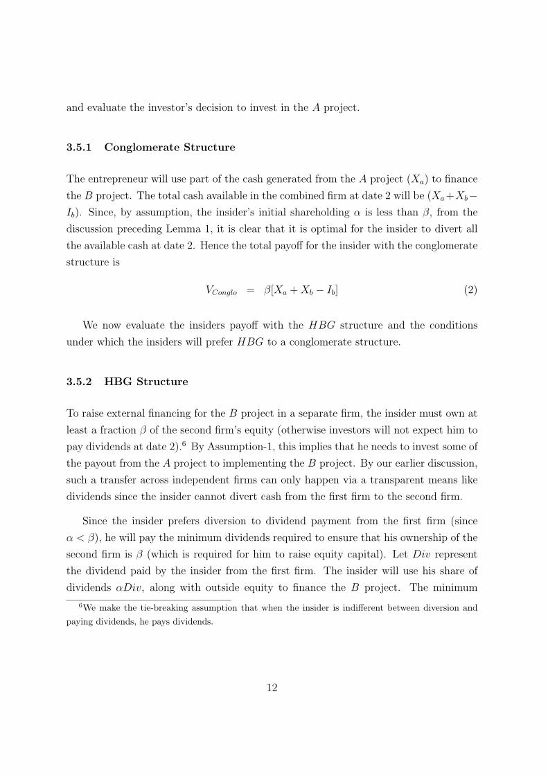
3.5.1 Conglomerate Structure

The entrepreneur will use part of the cash generated from the A project (Xa) to finance

the B project. The total cash available in the combined firm at date 2 will be (Xa+Xb−Ib). Since, by assumption, the insider’s initial shareholding α is less than β, from the

discussion preceding Lemma 1, it is clear that it is optimal for the insider to divert all

the available cash at date 2. Hence the total payoff for the insider with the conglomerate

structure is

VConglo = β[Xa + Xb − Ib] (2)

We now evaluate the insiders payoff with the HBG structure and the conditions

under which the insiders will prefer HBG to a conglomerate structure.

3.5.2 HBG Structure

To raise external financing for the B project in a separate firm, the insider must own at

least a fraction β of the second firm’s equity (otherwise investors will not expect him to

pay dividends at date 2).6 By Assumption-1, this implies that he needs to invest some of

the payout from the A project to implementing the B project. By our earlier discussion,

such a transfer across independent firms can only happen via a transparent means like

dividends since the insider cannot divert cash from the first firm to the second firm.

Since the insider prefers diversion to dividend payment from the first firm (since

α < β), he will pay the minimum dividends required to ensure that his ownership of the

second firm is β (which is required for him to raise equity capital). Let Div represent

the dividend paid by the insider from the first firm. The insider will use his share of

dividends αDiv, along with outside equity to finance the B project. The minimum

6We make the tie-breaking assumption that when the insider is indifferent between diversion andpaying dividends, he pays dividends.

12

dividend required to be paid from the first firm can be given as

β =Xb + αDiv − Ib

Xb

or Div =Ib − [1− β]Xb

α(3)

After paying a dividend of Div, the insider diverts any cash that remains from the A

project. Since the insider’s ownership in the second firm is β he will pay all the date 2

cash flows from the B project as dividends.

If both projects are financed, the total payoff to the insider from the HBG structure

is a sum of his payoff from the A project and the B project. This can be expressed as

follows:

VHBG = αDiv + β[Xa −Div] + Xb − Ib (4)

The insider’s payoff from the A project is a sum of his share of dividends and the

amount diverted. His payoff from the B project is the net present value of the project.

The following Proposition characterizes the insider’s choice between the two structures:

Proposition 1:

When Xa ≥ Ib, the insider will choose the HBG structure at date 1 and pay dividends

from the first firm iff:

α ≥ α∗ (5)

where

α∗ =Ib −Xb[1− β]

Ib

< β

With a single project, the minimum insider holding required to prevent diversion

is α = β (Lemma 1). Proposition 1 shows that in the presence of a second project,

with a HBG structure, the minimum insider holding required in the first firm to ensure

dividend payment is less than β. The intuition for the result is as follows. When choosing

between the conglomerate and the HBG structures, the insider trades off the loss due

to diversion in the conglomerate structure – with the loss from paying dividends to the

outside shareholders of the A project in the HBG structure. Although the marginal

13

cost of dividends is more than the marginal cost of diversion (since α < β) – the total

cost of diversion is the sum of the cost of diverting the A and B project resources while

the cost of paying dividends are confined to the A project. Therefore, even when α < β,

the insider might prefer the HBG structure.

We now turn to the financing at date 0, taking account of the expected decisions of

the insider at dates 1 and 2. If the insider chooses the conglomerate structure at date 1,

he does not pay any dividends from the A project. Anticipating this, investors will not

be willing to finance the A project. Thus in our model the entrepreneur will be able to

finance the A project only if he is expected to choose the HBG over the conglomerate

structure at date 1.

When the entrepreneur is expected to choose the HBG structure at date 1, the total

dividend paid by the first firm at date 1 is Div = Ib−[1−β]Xb

α. The dividend is paid only if

the insider gets the B project, which occurs with a probability p.7 The outside investors

get 1−α fraction of this dividend. Thus the total expected payoff of the outside investor

is p[1 − α]Div. The outside investors will be willing to invest in the A project as long

as this payoff is greater than the initial financing raised. That is:

p[1− α]Div ≥ Ia (6)

The following proposition states the conditions under which financing is possible for

both projects A and B:

Proposition 2:

(a). When Xa ≥ Ib, financing is feasible at date 0 for the two projects taken under

HBG structure iff:

Ia ≤ [1− β]Xb (7)

(b). When Xa < Ib financing is feasible for the two projects iff:

Ia ≤ pXa − p[Ib −Xb{1− β}] (8)

7If the insider does not get the B project, he does not pay dividends from the first firm as hisshareholding is less than β.

14

Proposition 2 indicates that there is an upper limit on the size of the A project

that can be financed i.e., not all positive NPV projects will be financed. As we might

expect, entrepreneurs are able to finance projects with lower profitability, if they have

a sufficiently high probability of getting a large second project. When Xa ≥ Ib, the

projects are funded only if (1 − β)Xb is large enough. The intuition is that outside

investors invest in the A project, anticipating the dividends to be paid at date 1. The

first firm pays dividends at date 1, only to enable the insider to finance the B project.

Consequently, the amount of dividend to be paid by the first firm, is proportional to the

size and profitability of the B project and so is the amount of investment that can be

financed in the A project. In the other case, when Ib > Xa, only the HBG structure is

feasible, as discussed. The conditions for the projects to be financed depend on the first

project payoff Xa and the relative profitability of the B project.

We have so far limited the insider’s choice at date 1 to a conglomerate structure and

a HBG structure. We now discuss the V BG structure in which, the first firm directly

invests in the equity of the second firm and the balance financing (if required) is raised

from outside investors. The following proposition extends our analysis to the V BG

structure.

Proposition 3:

(a). When Xa ≥ Ib, the insider’s payoff at date 1 with a V BG structure is equal to his

payoff with the conglomerate structure.

(b). When Xa < Ib, the insider will not be able to implement the B project using the

V BG structure.

This proposition establishes the equivalence of the V BG structure to the conglomer-

ate structure. The intuition for this proposition is as follows. When Xa ≥ Ib, the insider

will not raise any additional outside financing in the second firm at date 1. Hence, divi-

dends from the second firm will only result in a transfer back to the first firm. Further,

the insider will divert all the cash from the first firm since α < β. Thus, the insider’s

payoff at date 1 will be equal to β times, the total cash generated in the A project

(Xa) plus the net present value of the B project (Xb − Ib); the same as that in the

conglomerate structure.

15

When Xa < Ib, the insider will have to finance the shortfall by raising outside equity

in the second firm. The insider will be able to raise this equity only if he can commit

to paying dividends from the second firm at date 2. Since the insider will divert any

cash returned by the second firm to the first firm in form of dividends, his payoff will be

larger if he diverts the cash from the second firm at date 2. Anticipating this, outside

investors will not be willing to invest in the second firm at date 1. Therefore, similar

to the conglomerate structure, the insider will not be able to implement the B project

using the V BG structure whenever Xa < Ib.

Proposition 3 establishes that in our setting the entrepreneur will not be able to

finance the projects using the V BG structure. Our conclusion on the sub-optimality

of the V BG structure may seem surprising, considering the fact that vertical business

groups are widely present in many emerging economies. The main reason for our result

is the assumption that the insider’s shareholding in the first firm is less than β. This

assumption is reasonable in the case of young entrepreneurs starting out with their first

firm. We expect V BG structures might be optimal when insiders wealth constraints are

not too severe and when control issues are important.

We next consider the empirical implications of the model. We will discuss the extent

to which some of these implications may also be implied by other reasons for dividend

payments, such as the reputation of the business group. As we have said, our model of

dividend payment in a group setting is not mutually exclusive of other explanations –

but it does have the virtue of generating some specific predictions that are not easily

obtained from, say, a reputation based explanation of dividend policy.

4 Empirical Predictions and Data

We now discuss the main predictions of our model and compare them with those implied

by other explanations for dividend payments by group firms, such as preserving or

enhancing group reputation by dividend payout. In our discussion, we refer to firms

that get the B project as group firms, and the rest as stand alone firms. Our first

prediction, compares the dividend rates of group and stand alone firms. In the model,

only group firms pay dividends from the A project at date 1 to finance the B project.

These firms also pay dividends at date 2 from the B project. In contrast, stand alone

16

firms, do not pay any dividends. Since there may be other motives, such as reputation

to pay dividends, our prediction is that ceteris paribus, group firms will have greater

incentive to pay dividends than stand alone firms. Stated formally, our first prediction

is:

Prediction 1: Group firms will distribute more dividends than stand-alone firms.

In our setting, group firms pay dividends primarily to enable the group insiders to

invest in the equity of the newer firms in the group. These funds are, in turn, used to

make physical investments in the newer firms. Hence we expect a positive association

between dividend payments by a group firm and the physical investments by other

member firms and with the insider’s equity investment in other member firms. While

we do not observe the incremental investment of group insiders in the equity of other

firms, we do observe the increase in book equity through external equity financing in the

other member firms.8 If the incremental outside equity capital raised by group firms is

correlated with the incremental equity investment by insiders in these firms, we expect a

positive association between dividend payments by group firms with the external equity

capital raised by other firms in the group.9 Our next two predictions pertain to this

channel of transfer of resources. Stated formally:

Prediction 2 (a): Dividends of a group firm will be positively associated with invest-

ments in other group member firms.

Prediction 2 (b): Dividends of a group firm will be positively associated with increase

in external equity financing in the other firms in the group.

Note that the first and the second predictions are consistent with firms paying div-

idends due to reputation concerns (Gomes (2000)). For instance, one can argue that

groups will care more about their reputation since they have multiple firms which might

have occasion to access the financial markets in the future. Due to their reputation

concerns, groups, with more investment opportunities, might pay more dividends than

stand alone firms. A reputation argument would also suggest that dividend payments

of firms in the group would be linked with the future investment opportunities faced by

8In the data we observe the fraction of insider holding in a firm. This fraction is not time varyingand, hence, does not allow us to estimate the exact incremental investment of insiders.

9They will be perfectly correlated if group insiders purchase the same fraction in all new equityofferings as their initial equity holding.

17

the group. Since it is reasonable to assume that any reputation based effects do not vary

year on year, in our tests for the second prediction, we employ firm fixed effects and

control for any reputation effects.10 We would like to emphasize that by including firm

fixed effects we test for a stronger implication of our second prediction – i.e., changes in

group firm dividends will be positively associated with changes in investments (financed

by equity) and changes in external equity financing in other firms in the group.

We next discuss the implications of our model for the distribution of insider holding

within group firms. It is instructive to note that these predictions are not easily obtained

from a reputation based explanation of dividend policy.

In our model the average insider holding for group firms, is the average of the insider

holding in the A project and the B project, while the average insider holding for stand

alone firms is just the insider holding in the A project. Since insider holding in the

B project (equal to β) is greater than the insider holding in the A project, our model

predicts that group firms will, on average, have a higher level of insider holding than

stand alone firms.

Prediction 3: The average insider holding will be higher for group firms than for stand

alone firms.

A more dynamic implication of the model is that group insiders build up their re-

sources with successive projects and use the resources to acquire a higher fraction of the

equity of subsequent projects. This suggests that as the group gets older, insiders with

their greater wealth, are able to acquire greater fractional holding in the younger firms.

Thus, ceteris paribus, insider holding should be higher for the younger firms in the group

than for the older firms. This constitutes our next prediction:

Prediction 4(a): Within a group, younger firms will have a higher level of insider

holding than older firms.

Finally, on the same note, since insiders use dividends from existing firms to finance

their equity investment in new firms, ceteris paribus, we would expect the level of insider

holding in younger firms in the group to be positively associated with dividends paid

out by older firms in the group. This observation constitutes our final prediction:

10Note that, since the variable identifying a group firm is not time varying, we will not be able to usefirm fixed effect in our tests pertaining to the first prediction.

18

Prediction 4(b): Insider holding of younger firms in the group will be positively asso-

ciated with average dividend payments from older member firms in the group.

4.1 Data

We test all our predictions on the firm level data from India since we have comprehensive

data on both group and stand alone firms. We also test the second and the fourth

prediction using data on group firms from five other emerging markets, namely Thailand,

Malaysia, Philippines, South Korea, and Taiwan. We are unable to test the first and the

third predictions for these countries since we do not have information on group affiliation

for all the publicly traded firms available in Thompson Analytics’ Worldscope database.

This restricts our analysis to firms for whom group identity can be determined. As

highlighted earlier, we choose all the countries where pyramiding is not a significant

phenomenon (Bertrand et al. (2002); Claessens et al. (2000)) and hence the public

firms in the business groups can be treated as HBGs.

The financial and stock price data on Indian firms is from Prowess, a database main-

tained by CMIE, Centre for Monitoring the Indian Economy. Prowess provides annual

financial statements of public and private Indian firms including balance sheet, profit and

loss and cash flow statements starting from 1989. We collected information under three

broad headings from Prowess: (i) financial ratios from the annual reports; (ii) group

affiliation and group financial data and (iii) industry affiliation and industry aggregate

data. For identifying group affiliation, we adopt Prowess’s classification. This group

affiliation has been previously used by Khanna and Palepu (2000) and by Bertrand et

al. (2002). The classification is based on a continuous monitoring of company announce-

ments and qualitative understanding of group-wise behavior of individual firms and not

based only on equity ownership. Such a broad based classification – as against a narrow

equity centered classification – is more representative of group affiliation. For identifying

industry affiliation, we adopt Prowess’s classification of firms into industries based on

their principal line of activity. We code the industry classification at a level equivalent

to 4 digit SIC. We have data on firms from 95 such industries. For our analysis, we

consider all non-government and non-foreign firms which have positive sales during any

of the years from 1989 to 2002.

19

The sample of firms for Thailand, Malaysia, Philippines, South Korea, and Taiwan

are from the database of group firms made available by Claessens et al. (2000) at the

web site of the Journal of Financial Economics. We use this specific sample because we

require information on firms that belong to the same group. For emerging market firms

this information is publicly available only in this data set. We augment the Claessens

et al. data with detailed financial information from Thompson Analytics’ Worldscope

database. We used the SEDOL identifier as provided by Claessens et al. to match the

firms to Worldscope. To augment our sample, we also match manually by company

names. We adopt Claessens et al. classification for identifying industry affiliation and

classify firms into 15 industries. Our final sample for these countries has 493 firms (1,600

firm years) with positive sales during any of the years from 1989 to 2002. In contrast,

our Indian firm data has nearly 20,000 firm year observations for group firms. To avoid

confounding of any economic inferences due to large differences in the size of the two

samples, we perform our tests separately in the samples from East Asia and India.

5 Empirical Results

5.1 Descriptive Statistics

In Panel A of Table I, we provide the summary statistics for our sample of Indian

firms. We have over 45,000 firm-year observations comprising of about 25,000 stand

alone firm-year observations and 20,000 group firm-year observations. Group firms are

significantly larger than stand alone firms. They are also more profitable as indicated

by EBIDTA/TA ratios. Table I indicates that group firms pay more dividends than

stand alone firms (27% vs 10%). Furthermore, among the firms making positive profits,

a higher proportion of group firms pay dividends than stand alone firms (75% vs 50%).

These results offer some preliminary evidence in support of our first prediction. We use

the percentage of promoter shareholding given in Prowess as a measure of insider holding.

Prowess also gives the percentage shareholding of Indian Financial Institutions, Other

Corporates, Foreign Institutional Investors and other public shareholders. We classify

the holding of Indian Financial Institutions as Institutional holding and that of public

shareholders as Public holding. We can also observe that group firms have higher insider

holding (48.3%) in comparison to stand alone firms (43.3%). Correspondingly, stand

20

alone firms have greater dispersed outside equity as measured by “Public Equity”. This

is in line with our third prediction. All the differences highlighted between the group

and stand alone firms are significant at 1% level.

In Panel B, we present the summary median characteristics of the sample of group

firms from five East Asian countries: Thailand, Malaysia, Korea, Taiwan and Philip-

pines. Overall our sample (in Panels A and B) has substantial variation in terms of

dividend paying group firms; the median characteristics are similar to those reported

elsewhere in the literature (Faccio et al. (2001)). Since these are only summary statis-

tics, for more meaningful comparisons, we next turn to multivariate analysis.

5.2 Dividend Payments By Group Firms

Our first prediction compares the amount of dividends paid by group firms relative to

stand-alone firms. To test Prediction 1, we follow La Porta et al. (2000) and construct

four measures of dividend payments. Dividends are defined as total cash dividends paid

to common shareholders. We code dividends to be zero for firms that have missing

information on dividends but have negative earnings.11 The measures we construct

are:(i) Dividend/EBIDTAt: Measured as the ratio between the total dividends paid in

year t and the earnings before interest and depreciation in year t; (ii) Dividend/PAT t

(Payout ratio): Measured as the ratio between the total dividends paid in year t and the

profit after tax in year t; (iii) Dividend/Sales t: Measured as the ratio between the total

dividends paid in year t and the total sales in year t and (iv) Dividend/CF t: Measured

as the ratio between the total dividends paid in year t and the total cash flow from

operations in year t. Total cash flows from operations is measured as the firm’s profit

after tax plus depreciation less increase in net working capital. We do not use dividend

yield (Dividend/Market Price of Shares) since we do not have market price data over

the full sample period to construct this measure reliably.

To test the prediction, we estimate the following panel OLS regression in Table II:

yit = β0 + β1Groupi + β2Sales Growthit + β3Sizeit

+ β4Debt/TAit + Time FE+ Industry FE, (9)

11We repeated our analysis after dropping these observations and our results are unaffected

21

where the i subscript indicates the firm and the t subscript, time. The dependent

variable yit is a measure of dividend payment by Firmi in year t and denotes Divi-

dend/EBIDTA in Column (1), Dividend/PAT in Column (2), Dividend/Sales in Column

(3) and Dividend/CF in Column (4). Group is a dummy variable which takes a value

of 1 if the firm belongs to a group and 0 if it is a stand-alone firm. In our regressions,

we include other variables to control for firm characteristics. Specifically, we control

for leverage (Debt/TA), measured as the ratio of debt to total assets, size of the firm

(Size), measured as the log of book value of total assets and firm’s investment oppor-

tunities (Sales Growth), proxied by the annual growth rate in sales (as in La Porta et

al. (2000), where it is argued that this variable avoids incompatibility of accounting

variables across countries). To ensure that our results are not affected by time trends or

industry characteristics, we estimate our model with time and industry fixed effects. We

report standard errors that are corrected for panel, hetroskedasticity and autocorrelation

(AR-1). Our findings indicate that, consistent with our first prediction, group firms pay

more dividends than stand alone firm (β1 > 0). This difference is robust to different

ways of measuring dividend payments (Column (1)-(4)) and is both statistically and

economically significant. For instance, from Column (1), we find that group firms pay

5% more of their PAT as dividends in comparison to stand-alone firms.

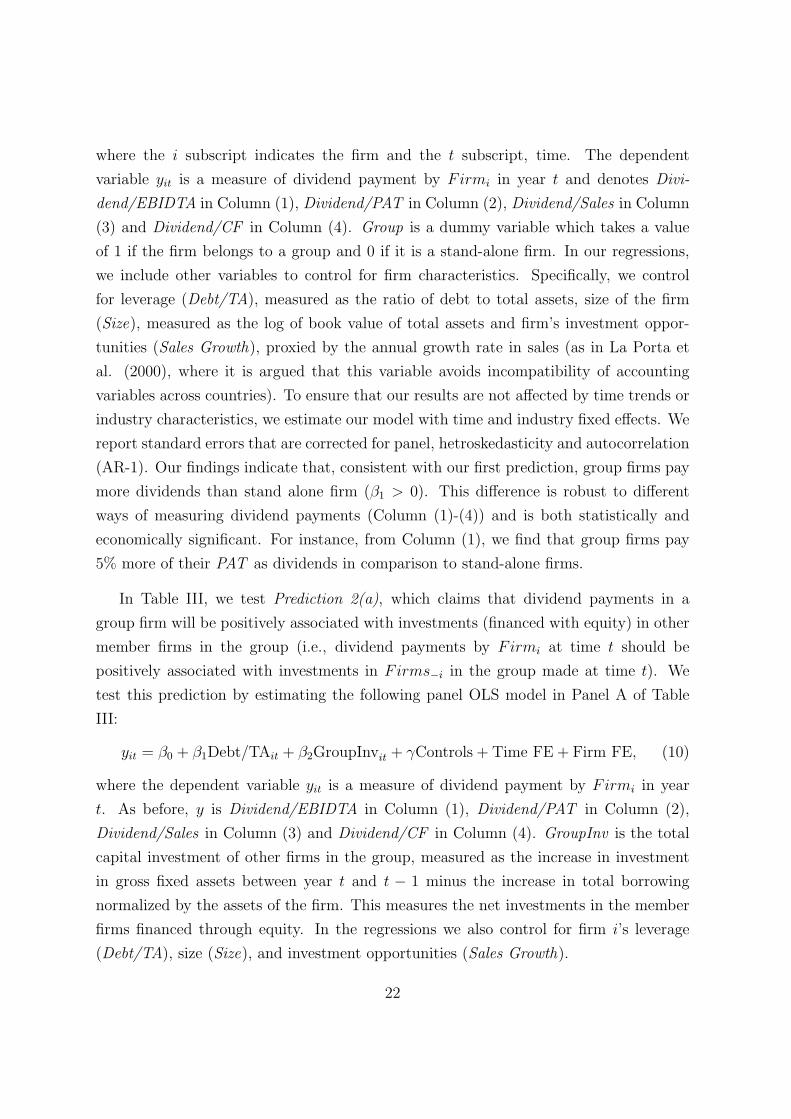
In Table III, we test Prediction 2(a), which claims that dividend payments in a

group firm will be positively associated with investments (financed with equity) in other

member firms in the group (i.e., dividend payments by Firmi at time t should be

positively associated with investments in Firms−i in the group made at time t). We

test this prediction by estimating the following panel OLS model in Panel A of Table

III:

yit = β0 + β1Debt/TAit + β2GroupInvit + γControls + Time FE + Firm FE, (10)

where the dependent variable yit is a measure of dividend payment by Firmi in year

t. As before, y is Dividend/EBIDTA in Column (1), Dividend/PAT in Column (2),

Dividend/Sales in Column (3) and Dividend/CF in Column (4). GroupInv is the total

capital investment of other firms in the group, measured as the increase in investment

in gross fixed assets between year t and t − 1 minus the increase in total borrowing

normalized by the assets of the firm. This measures the net investments in the member

firms financed through equity. In the regressions we also control for firm i’s leverage

(Debt/TA), size (Size), and investment opportunities (Sales Growth).

22

As highlighted in Section 4, a positive association between dividend payments and

investments in member firms can also arise due to unobserved differences in group ability

and/or its reputation attributes. Inclusion of firm fixed effects helps us overcome this

problem. Any positive association we capture would be on account of correlated time

series changes in dividends and group investments. This would be consistent with our

model but would not be predicted by a firm reputation based story. We report standard

errors that are corrected for panel, hetroskedasticity, and autocorrelation (AR-1). Our

coefficient of interest is β2 and our model predicts that this should be positive. Results in

Table III indicate that β2 is positive and significant for all the four measures of dividends

offering strong support for our prediction.

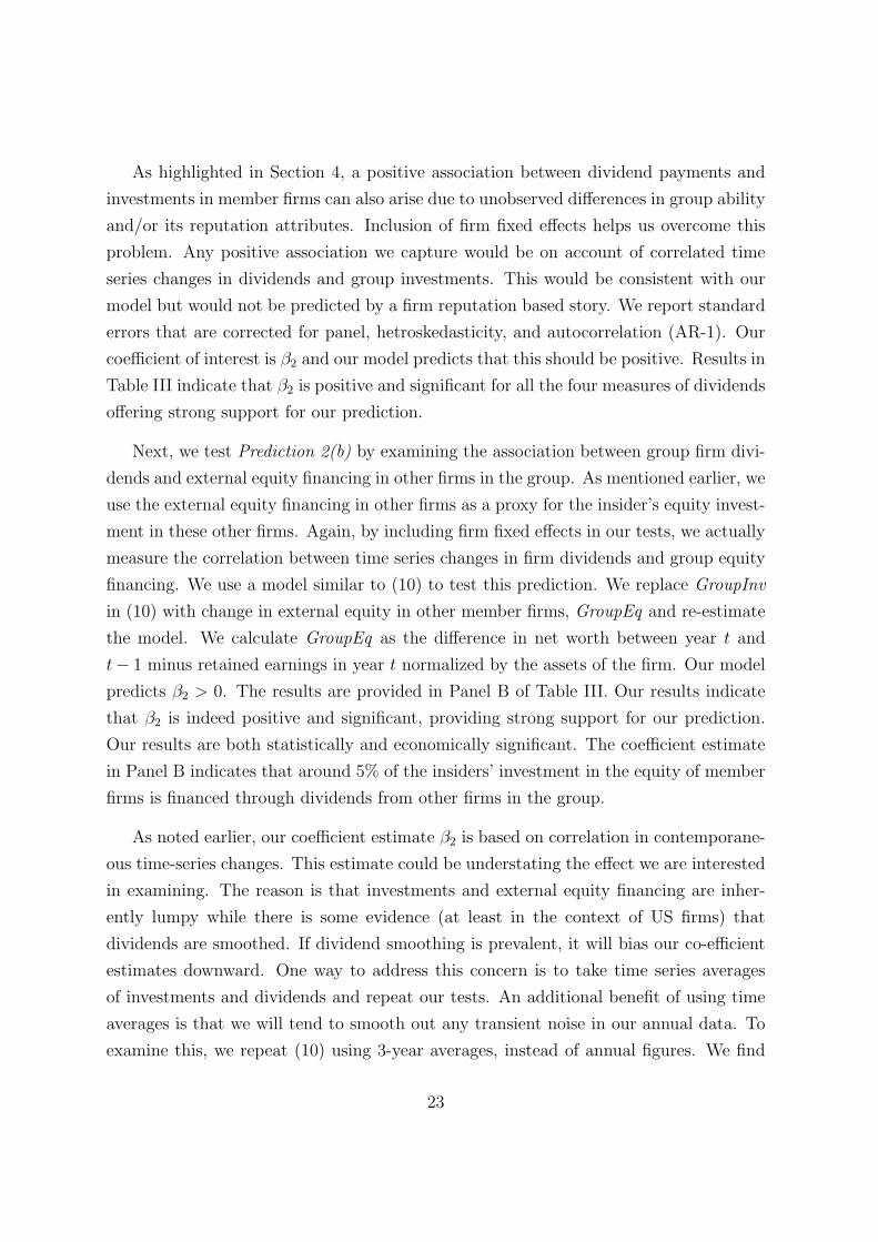
Next, we test Prediction 2(b) by examining the association between group firm divi-

dends and external equity financing in other firms in the group. As mentioned earlier, we

use the external equity financing in other firms as a proxy for the insider’s equity invest-

ment in these other firms. Again, by including firm fixed effects in our tests, we actually

measure the correlation between time series changes in firm dividends and group equity

financing. We use a model similar to (10) to test this prediction. We replace GroupInv

in (10) with change in external equity in other member firms, GroupEq and re-estimate

the model. We calculate GroupEq as the difference in net worth between year t and

t− 1 minus retained earnings in year t normalized by the assets of the firm. Our model

predicts β2 > 0. The results are provided in Panel B of Table III. Our results indicate

that β2 is indeed positive and significant, providing strong support for our prediction.

Our results are both statistically and economically significant. The coefficient estimate

in Panel B indicates that around 5% of the insiders’ investment in the equity of member

firms is financed through dividends from other firms in the group.

As noted earlier, our coefficient estimate β2 is based on correlation in contemporane-

ous time-series changes. This estimate could be understating the effect we are interested

in examining. The reason is that investments and external equity financing are inher-

ently lumpy while there is some evidence (at least in the context of US firms) that

dividends are smoothed. If dividend smoothing is prevalent, it will bias our co-efficient

estimates downward. One way to address this concern is to take time series averages

of investments and dividends and repeat our tests. An additional benefit of using time

averages is that we will tend to smooth out any transient noise in our annual data. To

examine this, we repeat (10) using 3-year averages, instead of annual figures. We find

23

that this procedure increases the magnitude of the coefficient estimate of interest (β3).

Specifically, our results indicate that 14% of the insiders’ investment in the equity of

member firms is financed through dividends from other firms in the group.

Using the data on group firms from five East Asian countries, we are able to test

Predictions 2(a) and 2(b). We use the same procedure as detailed above and report the

results of these tests in Table IV. As can be seen from Panel A and B of Table IV, our

results are qualitatively similar to those in Table III. Our results indicate that dividend

payments are significantly and positively associated with increases in group investments

and external equity in other member firms in these countries as well.

Our theoretical analysis shows that groups will use dividends to transfer cash from

cash surplus firms into cash deficit firms. In our test of this prediction (Prediction 2 ), we

do not measure the relationship separately for firms with better investment opportunities

(i.e., cash deficit) and those with poor investment opportunities (i.e., cash surplus).

We can design a sharper test of our second prediction if we can employ an exogenous

proxy for a firm’s investment opportunity. One potential proxy is Sales Growth that we

previously used. However, we feel that firm’s age would be a proxy closer in spirit to

our theoretical analysis. It can be argued that, in general, younger firms have greater

investment opportunities and, hence, are more likely to be in need of cash.12 This

would suggest that dividends from older firms in the group would be more sensitive to

investments and external equity financing in other firms in the group. To formally test

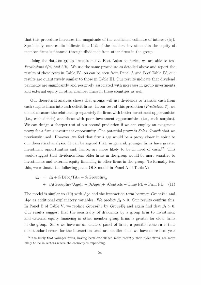
this, we estimate the following panel OLS model in Panel A of Table V:

yit = β0 + β1Debt/TAit + β2GroupInvit

+ β3(GroupInv*Age)it + β4Ageit + γControls + Time FE + Firm FE, (11)

The model is similar to (10) with Age and the interaction term between GroupInv and

Age as additional explanatory variables. We predict β3 > 0. Our results confirm this.

In Panel B of Table V, we replace GroupInv by GroupEq and again find that β3 > 0.

Our results suggest that the sensitivity of dividends by a group firm to investment

and external equity financing in other member group firms is greater for older firms

in the group. Since we have an unbalanced panel of firms, a possible concern is that

our standard errors for the interaction term are smaller since we have more firm year

12It is likely that younger firms, having been established more recently than older firms, are morelikely to be in sectors where the economy is expanding.

24

observations for the older firms than the younger firms in the group. To mitigate this

concern, we repeat our regressions using a balanced panel of firms and obtain similar

estimates to those reported. We estimate equation (11) using the data from five East-

Asian countries and find qualitatively similar results (Panels A and Panel B of Table

VI).

5.3 Distribution of Insider Holding in Group Firms

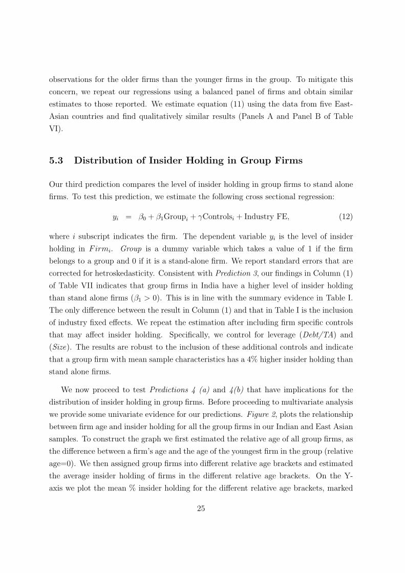
Our third prediction compares the level of insider holding in group firms to stand alone

firms. To test this prediction, we estimate the following cross sectional regression:

yi = β0 + β1Groupi + γControlsi + Industry FE, (12)

where i subscript indicates the firm. The dependent variable yi is the level of insider

holding in Firmi. Group is a dummy variable which takes a value of 1 if the firm

belongs to a group and 0 if it is a stand-alone firm. We report standard errors that are

corrected for hetroskedasticity. Consistent with Prediction 3, our findings in Column (1)

of Table VII indicates that group firms in India have a higher level of insider holding

than stand alone firms (β1 > 0). This is in line with the summary evidence in Table I.

The only difference between the result in Column (1) and that in Table I is the inclusion

of industry fixed effects. We repeat the estimation after including firm specific controls

that may affect insider holding. Specifically, we control for leverage (Debt/TA) and

(Size). The results are robust to the inclusion of these additional controls and indicate

that a group firm with mean sample characteristics has a 4% higher insider holding than

stand alone firms.

We now proceed to test Predictions 4 (a) and 4(b) that have implications for the

distribution of insider holding in group firms. Before proceeding to multivariate analysis

we provide some univariate evidence for our predictions. Figure 2, plots the relationship

between firm age and insider holding for all the group firms in our Indian and East Asian

samples. To construct the graph we first estimated the relative age of all group firms, as

the difference between a firm’s age and the age of the youngest firm in the group (relative

age=0). We then assigned group firms into different relative age brackets and estimated

the average insider holding of firms in the different relative age brackets. On the Y-

axis we plot the mean % insider holding for the different relative age brackets, marked

25

on the X-axis. The figure indicates that within a group, insider holding monotonically

decreases with firm age. For instance, in India, a group firm that is 25 years older than

the youngest firm in the group has, on average, 20% lower insider holding than the

youngest firm. This difference is statistically significant at 1% level. We find a similar,

though less pronounced, pattern between the age of a group firm and insider holding for

the sample from the five East-Asian countries (bottom graph in Figure 2 ).

To test Prediction 4(a) more formally, we estimate the following cross-sectional spec-

ification for group firms:

Insi = β0 + β1 ∗ (Debt/TA)i + β2 ∗ Sizei + β3 ∗ Agei

+ β4 ∗ EBIDTAi + Group FE, (13)

where Ins is the insider holding in a group firm and Age is the relative age of a group firm.

We control for other firm specific characteristics that could impact the level of insider

holding and include Debt/TA, EBIDTA, and Size. Finally, to capture unobserved group

characteristics that might influence the level of insider holding, we include group fixed

effects. We report standard errors that are hetroskedasticity consistent. We estimate

the model without any controls and report the results in Column (1) of Table VIII.

Our result indicates that, consistent with our prediction (4(a)), insider holding in group

firms decreases with firm age (β3 < 0). The coefficient estimate indicates that a firm

with mean sample characteristics that is 10 years older than the youngest firm in the

group, has a 10% lower insider holding than the average insider holding in the group.

This is a significant number given that the median insider holding in the group firms in

our sample is 48%.

We now test Prediction 4(b) which claims that the insider holding of young firms in

the group will be positively related to dividends paid out by the older firms in the group.

Specifically, we estimate the following cross-sectional regression for only the young firms

in the group – those with age less than the median age in the group.

Insi = β0 + β1 ∗ (Debt/TA)i + β2 ∗Sizei + β3 ∗Divi,o + β4 ∗EBIDTAi + β5 ∗NOF, (14)

Ins is the insider holding in the group firm and Divo represents the mean dividends paid

out by older firms in the group. In the regression we include, Debt/TA, EBIDTA and

Size. We also include NOF, representing the number of firms in the group. Standard

errors reported in parenthesis are heteroskedasticity consistent and are clustered at a

26

group level to ensure that our standard errors do not suffer from the downward bias that

is introduced by estimating effects of aggregate explanatory variables on individual-

specific response variables (Moulton (1990)). The results are given in Column (2) of

Table VIII and indicate that β3 is positive and significant. This suggests that insider

holdings in younger firms is positively associated with dividends paid by the older firms

in the group offering support for our prediction.

We test Predictions 4(a) and 4(b) using the data from five East-Asian countries.

Results from Panel A and Panel B of Table IX indicate that our results are consistent

with those from Table VIII.13 We next discuss the results from various robustness tests.

6 Robustness

We now subject our main results to several robustness tests. Specifically, we extend our

analysis to investigate if some of our results are driven by alternate explanations, data

limitations or our model specification.

Using a sample of Indian firms similar to ours, Bertrand et al. (2002) document

that Indian business groups tunnel cash from firms in which insiders have low cash flow

rights into firms in which they have high cash flow rights. An implicit assumption in the

tunnelling hypothesis is that the cash accumulated in the high cash flow rights firms will

(eventually) be distributed in the form of dividends. The tunnelling hypothesis would

predict that groups pay dividends predominantly from the high insider holding firms

and that these dividends should be related to the profits of low insider holding firms

in the group (controlling for the firm’s own profits). A possible concern may be that

the association we find between GroupInv, GroupEq and different measures of dividends

(Prediction 2(a) and 2(b)) is being driven by tunnelling in business groups. This may

occur if the dividends in our sample are paid mainly by high insider holding firms and

if changes in GroupInv and GroupEq are positively related to the changes in the profits

13To examine if the correlation between insider holding and dividends are due to some unobservedgroup level effect, we re-estimate (14) by switching young and old firms. That is, we estimate therelationship between insider holding in the older firms of the group and dividends paid by the youngerfirms in the group. We find that the coefficient estimate β3 is positive but insignificant. This offersfurther support that the direction of association is from dividends in old to insider holding in the young.

27

of low insider holding firms.

To evaluate this possibility, we re-estimate (10) for firms in the group with insider

ownership in the top 75th percentile. In our estimation, we also include total profits of

the low 25th percentile insider ownership firms in the group, LowProf, normalized by

their assets. We find that our results in Table III and IV are qualitatively unchanged.14

Hence, the results do not appear to be caused by dividend patterns that may be predicted

by the presence of tunnelling. We also examine alternatives to the proxy for investment

opportunity that we employed in our regressions. So far we have used the annual growth

rate in sales as a proxy for investment opportunities. Following La Porta et al. (2000),

we re-estimated our results using growth rates of assets and cash flows and find that our

results are unaffected. We also use industry adjusted dividends (on lines of La Porta et

al. (2000) and Faccio et al. (2001)) and find our results to be unchanged.

Next, we investigate the possible impact of not having time series insider holding

data. While the insider holding data that we use is from the most recent firm disclosures,

our theoretical predictions are based on insider’s holding at the time of firm’s inception.

Depending on whether insiders increase or decrease their holdings since the inception

of these firms, our data on their holdings could be higher or lower than the initial

holding. A possible scenario is that insiders dilute their initial stakes as firms get older

and mature, and consequently our insider holding data understates the level of insider

holding for older firms at the time of their inception. As a consequence, even if insiders

had the same level of holding in all the firms in the group at the time of formation, we

would mechanically find a negative relationship between insider holding and firm age.

A potential way to address this issue is to determine the relationship between firm age

and insider holding for stand alone firms. If the negative relationship we find for group

firms is driven by progressive divestiture of insider holding in older firms, we might expect

to find a similar negative relationship for stand alone firms. We investigate this for our

sample of stand-alone firms in India. In univariate analysis, we find no such relationship

for stand-alone firms. To ensure that this result is not different in a multivariate setting,

we re-estimate (14) for stand alone firms and find that the coefficient estimate on Age

is insignificant. These tests (unreported) suggest that our results are not driven by any

14Specifically, in our regressions for the Indian sample of firms, we find that LowProf is negative andinsignificant. This result is qualitatively unchanged when we use different measures of dividends.

28

mechanical divestiture by insiders as firms become older.

Next, instead of firm fixed effects we use the first difference procedure (Wooldridge

(2002)) for testing our second prediction. This addresses the concern that the fixed

effects estimator might be biased due to serial correlation of firm characteristics. From

the perspective of economic inference, this is a concern for us since firm fixed effects are

intended to control for slow-changing firm reputation effects. We re-estimate (10) using

first differences and find that our results are unchanged.

Finally, to alleviate concerns that our results may be affected by a particular time

period in the sample, we re-estimate all regressions for the subperiods 1989-1995 and

1996-2002. The results are qualitatively similar in the two subperiods.

7 Conclusion

In this paper, we offer a theory of dividends and financing with outside equity capital in

weak legal environments. We argue that business group insiders can use firm dividends as

a transparent means of transferring resources across firms in the group. These dividends

in turn sustain outside equity. We formalize this intuition in a model, endogenizing the

business group structure and develop predictions on both dividend policy and insider

holding in group firms. Our model of dividend payments in a group setting is not

mutually exclusive of other explanations such as firm or group reputation for paying

dividends to investors. However, it does have the virtue of generating some specific

predictions on the distribution of insider holding that are not easily obtained from, say,

a reputation based explanation of dividend policy.

The model’s main predictions are: (i) Group firms should pay more in dividends and

have more insider ownership than stand alone firms; (ii) Dividends of a group firm should

be positively associated with investment and external equity financing in other member

firms in its group and (iii) Younger firms in a group should have more insider holding than

older firms; insider holding in the young firms in the group should be positively related

to dividend distribution from the group’s older firms. These predictions are tested on

detailed firm level data for six emerging economies. We find substantial support for each

of the our predictions, supporting the notion business groups in emerging markets use

29

dividends as a transparent way of transferring cash across group firms.

In our view the results in the model indicate a type of “second best” equilibrium.

Weak legal rights and poor enforcement make it difficult for entrepreneurs to raise out-

side financing. However, they may be able to partially offset some of these limitations by

developing organizational structures that enhance their ability to raise outside financ-

ing. The paper generates some policy implications. An obvious one is that enhanced

investor rights and improved enforcement will enable firms to raise more outside capital:

interestingly the model suggests that this may well be accompanied by a reduction in

the dividend payout and, possibly, less reliance on the business group structure. The

paper also suggests that it may be important – even without an improvement in investor

rights – to make it difficult for insiders to consume or invest significant sums, unless the

source of the funds is disclosed. The rationale is that if insiders are unable to reinvest or

consume the resources they divert, they may limit their diversion and may employ means

like dividends to transfer resources. In the end, this makes it easier for entrepreneurs to

raise outside capital.

30

References

Almeida, Heitor and Daniel Wolfenzon, (2004), “A Theory of Pyramidal Ownership and Family Business Groups”,

New York University Working Paper.

Bae, Kee-Hong, Jun-Koo Kang and Jin-Mo Kim, (2002), “Tunneling or Value Added? Evidence From Mergers

by Korean Business Groups”, Journal of Finance, 57 (6), 2695-2740.

Bertrand, Marianne, Paras Mehta and Sendhil Mullainathan (2002), “Ferreting Out Tunnelling: An Application

to Indian Business Groups”, Quarterly Journal of Economics, 117 (1), 121-148.

Burkart, Mike C., Fausto Panunzi and Andrei Shleifer , (2003), “Family Firms” Journal of Finance, 58 (5),

2167-2201.

Claessens, Stijn, Simeon Djankov, Joseph, P.H. Fan, and Larry H.P. Lang (2002), “Disentangling the Incentive

and Entrenchment Effects of Large Shareholders”, Journal of Finance, 51 (6), 2741-2771.

Claessens, Stijn, Simeon Djankov and Larry H.P. Lang, (2000), “The Separation of Ownership and Control in

East Asian Corporations”, Journal of Financial Economics, 58 (1-2), 81-112.

Desai, Mihir, A., Alexander Dyck and Luigi Zingales (2004), “Theft and Taxes”, University of Chicago Working

Paper.

Durnev, Art, Han E. Kim (forthcoming), “To Steal or Not to Steal: Firm Attributes, Legal Environment, and

Valuation”, Journal of Finance.

Easterbrook, Frank H., (1984), “Agency-Cost Explanations of Dividends”, American Economic Review, 74 (4),

650-659.

Faccio, Mara, Larry, H.P. Lang and Leslie Young, (2001), “Dividends and Expropriation”, American Economic

Review, 91 (1), 54-78.

Fluck, Zsuzsanna, (1998), “Optimal Financial Contracting: Debt Versus Outside Equity”, Review of Financial

Studies, 11 (2), 383-418.

Fluck, Zsuzsanna, (1999), “The Dynamics of the Management-Shareholder Conflict”, Review of Financial Studies,

12 (2), 379-404.

Friedman, Eric, Simon Johnson and Todd Mitton, (2003), “Propping and Tunneling,” NBER Working Paper

9949.

Gopalan, Radhakrishnan, Vikram Nanda and Amit Seru (2004), “Business Groups and Bankruptcy Spillovers”,

University of Michigan Working Paper.

Gomes, Armando, (2000), “Going Public Without Governance: Managerial Reputation Effects”, Journal of

Finance, 55 (2), 615-646.

Grossman, Sandy and Oliver Hart, (1986), “The Costs and Benefits of Ownership: A Theory of Vertical and

Lateral Integration”, Journal of Political Economy, 94(4), 691-719.

31

Hart, Oliver, (1995), Firms Contracts and Financial Structure, Oxford: Clarendon Press.

Hart, Oliver and John Moore, (1994), “A Theory of Debt Based on the Inalienability of Human-Capital”, Quarterly

Journal of Economics, 109 (4), 841-879.

Jensen, Michael, (1986), “Agency Costs of Free Cash Flow, Corporate-Finance and Takeovers”, American Eco-

nomic Review, 76 (2), 323-329.

Jensen, Michael and William Meckling, (1976), Theory of Firm - Managerial Behavior, Agency Costs and Own-

ership Structure”, Journal of Financial Economics, 3 (4), 305-360.

Kali, Raja (2002), “Contractual Governance, Business Groups and Transition”, Economics of Transition, 10 (2),

255-272.

Khanna, Tarun, and Krishna Palepu, (2000), “Is Group Affiliation Profitable in Emerging Markets? An Analysis

of Diversified Indian Business Groups”, Journal of Finance, 55 (2), 867 - 891.

Khanna, Tarun and Yishay Yafeh (forthcoming),“Business Groups and Risk Sharing Around the World”, Journal

of Business.

La Porta Rafael, Florencio Lopez-de-Silanes, Andrei Shleifer and Robert Vishny (1998), “Law and Finance”,

Journal of Political Economy, 106 (6), 1113-1155.

La Porta Rafael, Florencio Lopez-de-Silanes, Andrei Shleifer and Robert W. Vishny, (2000), “Agency Problems

and Dividend Policies Around the World”, Journal of Finance, 55 (1), 1-33.

Miller, Merton, H and Myron S. Scholes, (1978), “Dividends and Taxes”, Journal of Financial Economics, 6 (4),

333-364.

Moulton, Brent, R., (1990), “An Illustration of a Pitfall in Estimating the Effects of Aggregate Variables on Micro

Units”, Review of Economics and Statistics,72 (2), 334-338.

Myers, Stewart C. (2000), “Outside Equity”, Journal of Finance, 55 (3), 1005-1037.

Shin, Hyun-Han. and Young S. Park, (1999) “Financing Constraints and Internal Capital Markets: Evidence

from Korean Chaebols”, Journal of Corporate Finance, 5 (2), 169 - 191.

Shleifer Andrei, Robert W. Vishny (1992), “Liquidation Values and Debt Capacity: A Market Equilibrium Ap-

proach”, Journal of Finance, 47 (4), 1343-1366.

Van der Molen, Lensink, R. and S. Gangopadhyay, (2003), “ Business groups, financing constraints and investment:

The case of India”, Journal of Development Studies, 40, 93-119.

Woolridge, Jeffrey, M., (2002), Econometric Analysis of Cross Section and Panel Data, Cambridge, MA: MIT

Press.

Zwiebel Jeffrey, (1996), “Dynamic Capital Structure Under Managerial Entrenchment”, American Economic

Review, 86 (5), 1197-1215.

32

A Appendix

A.1 Proof of Lemma 1

The entrepreneur will choose to pay dividends if α ≥ β. The extent of entrepreneur’s shareholding in the project is

determined by the individual rationality constraint of outside shareholders. That is given as:

[1− α]Xa = Ia

α =Xa − Ia

Xa(A-1)

The condition required to ensure dividends is α ≥ β. Substituting for α we have:

Xa − Ia

Xa≥ β (A-2)

Q.E.D.

A.2 Proof of Proposition 1

The entrepreneur will choose the structure that will maximize his payoff. Comparing the payoffs of the insider from the

HBG and conglomerate structures, the insider will choose the HBG structure if:

αDiv + β[Xa −Div] + Xb − Ib ≥ β[Xa + Xb − Ib]

or Ib − [1− β]Xb + β{Xa − Ib − [1− β]Xb

α}+ Xb − Ib ≥ β[Xa + Xb − Ib]

which can be simplified toIb − [1− β]Xb

α≤ Ib

or α ≥ Ib −Xb[1− β]

Ib(A-3)

We can show thatIb−Xb[1−β]

Ib< β as follows. To show

Ib −Xb[1− β]

Ib< β

or to show Ib[1− β]−Xb[1− β] < 0

The last inequality is true from our assumption that the B project has positive NPV Q.E.D.

A.3 Proof of Proposition 2

Substituting for Div in (6), a necessary condition for financing of the A project is

p[1− α]Ib −Xb[1− β]

α≥ Ia

or α ≤ p{Ib −Xb[1− β]}Ia + p{Ib −Xb[1− β]} (A-4)

33

Combining (A-4) and (A-3) we have

p{Ib −Xb[1− β]}Ia + p{Ib −Xb[1− β]} ≥ Ib −Xb[1− β]

Ib

or 0 ≥ Ia − p[1− β]Xb

p[1− β]Xb ≥ Ia (A-5)

To prove the second part of the proposition, we consider the case when Xa < Ib. As discussed in the text the conglomerate

structure is not feasible in this case. The entrepreneur will always choose the HBG structure whenever he gets the B

project. The minimum dividend that he will have to pay for implementing the second project still remains Div given by

(3). This is feasible as long as Div ≤ Xa. Or

Ib − [1− β]Xb

α≤ Xa

α ≤ Ib − [1− β]Xb

Xa(A-6)

Combing the above inequality with (A-4) we have

p{Ib −Xb[1− β]}Ia + p{Ib −Xb[1− β]} ≥ Ib − [1− β]Xb

Xa

or Ia ≤ pXa − p{Ib −Xb[1− β]} (A-7)

Q.E.D.

A.4 Proof of Proposition 3

In the V BG structure, the first firm will directly invest in the second firm implementing the B project. When Xa ≥ Ib

the second firm will be a wholly owned subsidiary of the first firm. In this case the equivalence of the V BG structure to

the conglomerate structure is obvious.

When Xa < Ib, additional outside equity has to be raised in the second firm to the extent of Ib−Xa. This is feasible

only if the insider can commit to paying dividends from the second firm at date 2. We now explore the insider’s incentives

to pay dividends from the second firm at date 2.

After raising the outside equity, the shareholding of the second firm will comprise of the first firm and outside

shareholders. Any dividends paid from the second firm will hence go to the first firm and outside shareholders. For the

outside shareholders in the second firm to break-even, their share of dividends must be Ib − Xa. The first firm’s share

will hence be Xb − Ib + Xa. The insider will divert all cash coming back to the first firm since α < β. Thus the insider’s

payoff if he pays dividends will be β[Xb − Ib + Xa]. Instead of paying dividends, if the insider were to divert all the cash

from the second firm his payoff will be βXb. The insider will pay dividends iff:

β[Xb − Ib + Xa] ≥ βXb

or Xa ≥ Ib (A-8)

But the last inequality is false because we are considering the case when Xa < Ib. Thus, the insider will not pay dividends

at date 2 and consequently no outside financing can be raised at date 1. Q.E.D.

34

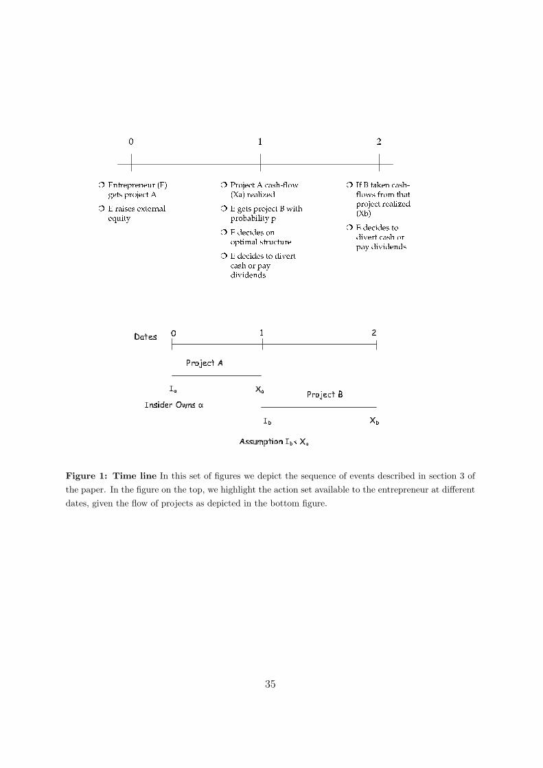
Figure 1: Time line In this set of figures we depict the sequence of events described in section 3 ofthe paper. In the figure on the top, we highlight the action set available to the entrepreneur at differentdates, given the flow of projects as depicted in the bottom figure.

35

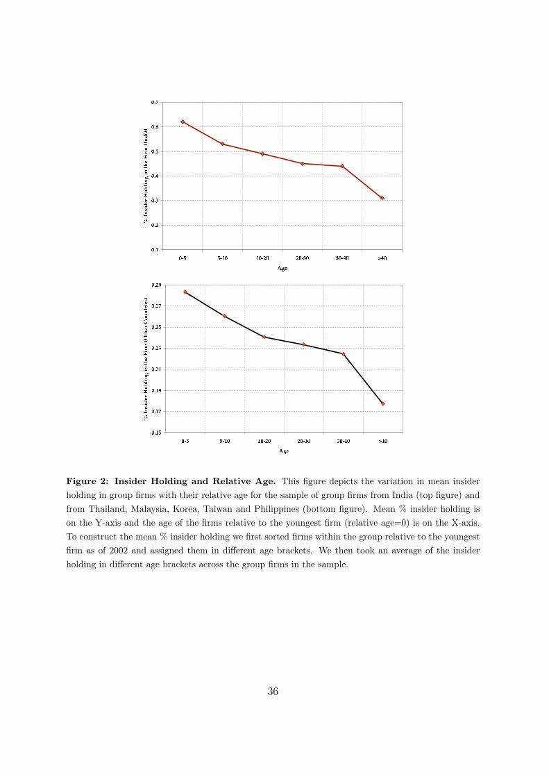
Figure 2: Insider Holding and Relative Age. This figure depicts the variation in mean insiderholding in group firms with their relative age for the sample of group firms from India (top figure) andfrom Thailand, Malaysia, Korea, Taiwan and Philippines (bottom figure). Mean % insider holding ison the Y-axis and the age of the firms relative to the youngest firm (relative age=0) is on the X-axis.To construct the mean % insider holding we first sorted firms within the group relative to the youngestfirm as of 2002 and assigned them in different age brackets. We then took an average of the insiderholding in different age brackets across the group firms in the sample.

36

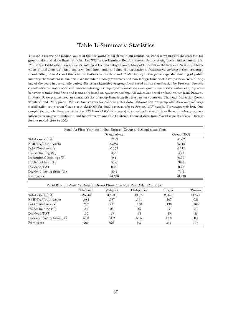
Table I: Summary Statistics

This table reports the median values of the key variables for firms in our sample. In Panel A we present the statistics for

group and stand alone firms in India. EBIDTA is the Earnings Before Interest, Depreciation, Taxes, and Amortization.

PAT is the Profit after Taxes, Insider holding is the percentage shareholding of Directors in the firm and Debt is the book

value of total short term and long term debt from banks and financial institutions. Institutional holding is the percentage

shareholding of banks and financial institutions in the firm and Public Equity is the percentage shareholding of public

minority shareholders in the firm. We include all non-government and non-foreign firms that have positive sales during

any of the years in our sample period. Firms are identified as group firms based on the classification by Prowess. Prowess

classification is based on a continuous monitoring of company announcements and qualitative understanding of group wise

behavior of individual firms and is not only based on equity ownership. All values are based on book values from Prowess.

In Panel B, we present median characteristics of group firms from five East Asian countries: Thailand, Malaysia, Korea,

Thailand and Philippines. We use two sources for collecting this data. Information on group affiliation and industry

classification comes from Claessens et al.(2000)(For details please refer to Journal of Financial Economics website). Our

sample for firms in these countries has 493 firms (1,600 firm years) since we include only those firms for whom we have

information on group affiliation and for whom we are able to obtain financial data from Worldscope database. Data is

for the period 1989 to 2002.

Panel A: Firm Years for Indian Data on Group and Stand alone Firms

Stand Alone Group (BG)

Total assets (TA) 126.9 512.2

EBIDTA/Total Assets 0.085 0.118

Debt/Total Assets 0.203 0.211

Insider holding (%) 43.2 48.3

Institutional holding (%) 0.1 6.00

Public holding (%) 52.6 39.6

Dividend/PAT 0.10 0.27

Dividend paying firms (%) 50.1 74.6

Firm years 24,520 20,916

Panel B: Firm Years for Data on Group Firms from Five East Asian Countries

Thailand Malaysia Philippines Korea Taiwan

Total assets (TA) 727.43 399.93 390.77 234.73 947.71

EBIDTA/Total Assets .084 .087 .101 .107 .021

Debt/Total Assets .287 .221 .150 .130 .106

Insider holding (%) 34 26 23 17 20

Dividend/PAT .30 .43 .32 .35 .28

Dividend paying firms (%) 50.3 54.2 55.5 47.9 60.1

Firm years 200 628 347 345 107

37

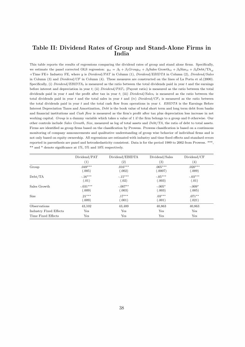
Table II: Dividend Rates of Group and Stand-Alone Firms inIndia

This table reports the results of regressions comparing the dividend rates of group and stand alone firms. Specifically,

we estimate the panel corrected OLS regression: yit = β0 + β1Groupit + β2Sales Growthit + β3Sizeit + β4Debt/TAit

+Time FE+ Industry FE, where y is Dividend/PAT in Column (1), Dividend/EBIDTA in Column (2), Dividend/Sales

in Column (3) and Dividend/CF in Column (4). These measures are constructed on the lines of La Porta et al.(2000).

Specifically, (i) Dividend/EBIDTAt is measured as the ratio between the total dividends paid in year t and the earnings

before interest and depreciation in year t; (ii) Dividend/PAT t (Payout ratio) is measured as the ratio between the total

dividends paid in year t and the profit after tax in year t; (iii) Dividend/Salest is measured as the ratio between the

total dividends paid in year t and the total sales in year t and (iv) Dividend/CF t is measured as the ratio between

the total dividends paid in year t and the total cash flow from operations in year t. EBIDTA is the Earnings Before

Interest Depreciation Taxes and Amortization, Debt is the book value of total short term and long term debt from banks

and financial institutions and Cash flow is measured as the firm’s profit after tax plus depreciation less increase in net

working capital. Group is a dummy variable which takes a value of 1 if the firm belongs to a group and 0 otherwise. Our

other controls include Sales Growth, Size, measured as log of total assets and Debt/TA, the ratio of debt to total assets.

Firms are identified as group firms based on the classification by Prowess. Prowess classification is based on a continuous

monitoring of company announcements and qualitative understanding of group wise behavior of individual firms and is

not only based on equity ownership. All regressions are estimated with industry and time fixed effects and standard errors

reported in parenthesis are panel and hetroskedasticity consistent. Data is for the period 1989 to 2002 from Prowess. ***,

** and * denote significance at 1%, 5% and 10% respectively.

Dividend/PAT Dividend/EBIDTA Dividend/Sales Dividend/CF

(1) (2) (3) (4)

Group .049∗∗∗ .016∗∗∗ .005∗∗∗ .020∗∗∗(.005) (.002) (.0007) (.009)

Debt/TA -.16∗∗∗ -.15∗∗∗ -.05∗∗∗ -.03∗∗∗(.01) (.02) (.003) (.01)

Sales Growth -.031∗∗∗ -.007∗∗ -.005∗ -.009∗(.009) (.003) (.003) (.005)

Size .21∗∗∗ .17∗∗∗ .03∗∗∗ .071∗∗(.009) (.001) (.001) (.021)

Observations 43,102 43,489 40,863 40,863

Industry Fixed Effects Yes Yes Yes Yes

Time Fixed Effects Yes Yes Yes Yes

38

Table III: Dividends, Investment, and External Equity inGroup Firms from India

This table reports the results of regressions relating dividend rates of one firm to increase in investment and external equity in other firms

in the group. Specifically, in Panel A we run the panel corrected OLS regression: yit = β0 + β1 ∗ (Debt/TA)it + β2 ∗ (GroupInv)it +

γControls+ Time FE+ Firm FE, where y is Dividend/EBIDTA in Column (1), Dividend/PAT in Column (2), Dividend/Sales in Column (3)

and Dividend/CF in Column (4). These measures are constructed on the lines of La Porta et al.(2000). Specifically, (i) Dividend/EBIDTAt is

measured as the ratio between the total dividends paid in year t and the earnings before interest and depreciation in year t; (ii) Dividend/PATt

(Payout ratio) is measured as the ratio between the total dividends paid in year t and the profit after tax in year t; (iii) Dividend/Salest is

measured as the ratio between the total dividends paid in year t and the total sales in year t and (iv) Dividend/CFt is measured as the ratio

between the total dividends paid in year t and the total cash flow from operations in year t. Total cash flows from operations is measured

as the firm’s profit after tax plus depreciation less increase in net working capital. EBIDTA is the Earnings Before Interest Depreciation

Taxes and Amortization, Debt is the book value of total short term and long term debt from banks and financial institutions, Cash flow is

measured as the firm’s profit after tax plus depreciation less increase in net working capital and GroupInv is the total capital investment

in the group, measured as the increase in investment in fixed assets between year t and t − 1 in other member firms minus the increase in

total borrowing in other member firms normalized by the total assets of the firm. In Panel B, we replace the variable GroupInv by increase

in external equity (GroupEq). We calculate this variable as difference in net worth between year t and t − 1 in other member firms minus

retained earnings in year t in other member firms, normalized by the assets of the firm. Other controls include Sales Growth, Size, measured

as log of total assets and Debt/TA, the ratio of debt to total assets. All regressions are estimated with firm fixed effects only on group

firms and the standard errors reported in parenthesis are panel and hetroskedasticity consistent. Data is for the period 1989 to 2002 from

Prowess. ***, ** and * denote significance at 1%, 5% and 10% respectively.

Panel A: Dividends and Group Investment

Dividend/EBIDTA Dividend/PAT Dividend/Sales Dividend/CF

(1) (2) (3) (4)

GroupInv .007∗∗ .006∗∗∗ .004∗∗∗ .009∗∗∗(.004) (.002) (.001) (.037)

Debt/TA -.089∗∗∗ -.183∗∗∗ -.022∗∗∗ -.13∗∗∗(.004) (.016) (.002) (.047)

Sales Growth .007 .006 .006 .006(.005) (.005) (.005) (.005)

Size 0.01∗∗ 0.02∗∗ 0.01∗∗ 0.01∗∗(.005) (.01) (.005) (.005)

Observations 15,852 15,793 14,990 14,990

Firm Fixed Effects Yes Yes Yes Yes

Time Fixed Effect Yes Yes Yes Yes

Panel B: Dividends and Increase in External Equity

Dividend/EBIDTA Dividend/PAT Dividend/Sales Dividend/CF

(1) (2) (3) (4)

GroupEq .009∗∗∗ .009∗∗∗ .010∗∗∗ .016∗∗∗(.003) (.002) (.001) (.029)

Debt/TA -.081∗∗∗ -.131∗∗∗ -.028∗∗∗ -.11∗∗∗(.004) (.016) (.002) (.047)

Sales Growth .006 .007 .005 .005(.005) (.005) (.005) (.005)

Size 0.01∗∗ 0.02∗∗ 0.01∗∗ 0.01∗∗(.004) (.01) (.004) (.004)

Observations 15,852 15,793 14,990 14,990

Firm Fixed Effects Yes Yes Yes Yes

Time Fixed Effect Yes Yes Yes Yes

39

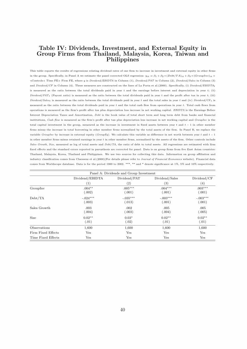
Table IV: Dividends, Investment, and External Equity inGroup Firms from Thailand, Malaysia, Korea, Taiwan and

Philippines

This table reports the results of regressions relating dividend rates of one firm to increase in investment and external equity in other firms

in the group. Specifically, in Panel A we estimate the panel corrected OLS regression: yit = β1 + β2 ∗ (Debt/TA)it + β3 ∗ (GroupInv)it +

γControls+ Time FE+ Firm FE, where y is Dividend/EBIDTA in Column (1), Dividend/PAT in Column (2), Dividend/Sales in Column (3)

and Dividend/CF in Column (4). These measures are constructed on the lines of La Porta et al.(2000). Specifically, (i) Dividend/EBIDTAt

is measured as the ratio between the total dividends paid in year t and the earnings before interest and depreciation in year t; (ii)

Dividend/PATt (Payout ratio) is measured as the ratio between the total dividends paid in year t and the profit after tax in year t; (iii)

Dividend/Salest is measured as the ratio between the total dividends paid in year t and the total sales in year t and (iv) Dividend/CFt is

measured as the ratio between the total dividends paid in year t and the total cash flow from operations in year t. Total cash flows from

operations is measured as the firm’s profit after tax plus depreciation less increase in net working capital. EBIDTA is the Earnings Before

Interest Depreciation Taxes and Amortization, Debt is the book value of total short term and long term debt from banks and financial

institutions, Cash flow is measured as the firm’s profit after tax plus depreciation less increase in net working capital and GroupInv is the

total capital investment in the group, measured as the increase in investment in fixed assets between year t and t − 1 in other member

firms minus the increase in total borrowing in other member firms normalized by the total assets of the firm. In Panel B, we replace the

variable GroupInv by increase in external equity (GroupEq). We calculate this variable as difference in net worth between year t and t − 1

in other member firms minus retained earnings in year t in other member firms, normalized by the assets of the firm. Other controls include

Sales Growth, Size, measured as log of total assets and Debt/TA, the ratio of debt to total assets. All regressions are estimated with firm

fixed effects and the standard errors reported in parenthesis are corrected for panel. Data is on group firms from five East Asian countries:

Thailand, Malaysia, Korea, Thailand and Philippines. We use two sources for collecting this data. Information on group affiliation and

industry classification comes from Claessens et al.(2000)(For details please refer to Journal of Financial Economics website). Financial data

comes from Worldscope database. Data is for the period 1989 to 2002. ***, ** and * denote significance at 1%, 5% and 10% respectively.

Panel A: Dividends and Group Investment

Dividend/EBIDTA Dividend/PAT Dividend/Sales Dividend/CF

(1) (2) (3) (4)

GroupInv .004∗∗ .005∗∗∗ .004∗∗∗ .003∗∗∗(.002) (.001) (.001) (.001)

Debt/TA -.024∗∗∗ -.035∗∗∗ -.003∗∗∗ -.003∗∗∗(.003) (.013) (.001) (.001)

Sales Growth .003 .002 .005 .005(.004) (.003) (.004) (.005)

Size 0.02∗∗ 0.03∗ 0.02∗∗ 0.02∗∗(.01) (.02) (.01) (.01)

Observations 1,600 1,600 1,600 1,600

Firm Fixed Effects Yes Yes Yes Yes

Time Fixed Effects Yes Yes Yes Yes

40

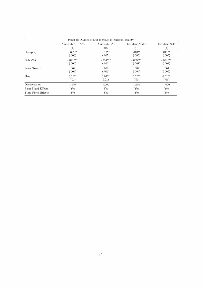
Panel B: Dividends and Increase in External Equity

Dividend/EBIDTA Dividend/PAT Dividend/Sales Dividend/CF

(1) (2) (3) (4)

GroupEq .006∗∗∗ .012∗∗ .010∗∗ .011∗∗(.003) (.005) (.005) (.005)

Debt/TA -.021∗∗∗ -.034∗∗∗ -.003∗∗∗ -.004∗∗∗(.005) (.012) (.001) (.001)

Sales Growth .002 .002 .004 .004(.004) (.003) (.004) (.005)

Size 0.02∗∗ 0.02∗∗ 0.02∗∗ 0.02∗∗(.01) (.01) (.01) (.01)

Observations 1,600 1,600 1,600 1,600

Firm Fixed Effects Yes Yes Yes Yes

Time Fixed Effects Yes Yes Yes Yes

41

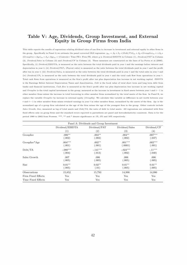
Table V: Age, Dividends, Group Investment, and ExternalEquity in Group Firms from India

This table reports the results of regressions relating dividend rates of one firm to increase in investment and external equity in other firms in

the group. Specifically in Panel A we estimate the panel corrected OLS regression: yit = β0 + β1 ∗ (Debt/TA)it + β2 ∗GroupInvit ++β3 ∗(GroupInv ∗Age)it + β4 ∗Ageit + γControls+ Time FE+ Firm FE, where y is Dividend/EBIDTA in Column (1), Dividend/PAT in Column

(2), Dividend/Sales in Column (3) and Dividend/CF in Column (4). These measures are constructed on the lines of La Porta et al.(2000).

Specifically, (i) Dividend/EBIDTAt is measured as the ratio between the total dividends paid in year t and the earnings before interest and

depreciation in year t; (ii) Dividend/PATt (Payout ratio) is measured as the ratio between the total dividends paid in year t and the profit

after tax in year t; (iii) Dividend/Salest is measured as the ratio between the total dividends paid in year t and the total sales in year t and

(iv) Dividend/CFt is measured as the ratio between the total dividends paid in year t and the total cash flow from operations in year t.

Total cash flows from operations is measured as the firm’s profit after tax plus depreciation less increase in net working capital. EBIDTA

is the Earnings Before Interest Depreciation Taxes and Amortization, Debt is the book value of total short term and long term debt from

banks and financial institutions, Cash flow is measured as the firm’s profit after tax plus depreciation less increase in net working capital

and GroupInv is the total capital investment in the group, measured as the increase in investment in fixed assets between year t and t− 1 in

other member firms minus the increase in total borrowing in other member firms normalized by the total assets of the firm. In Panel B, we

replace the variable GroupInv by increase in external equity (GroupEq). We calculate this variable as difference in net worth between year

t and t− 1 in other member firms minus retained earnings in year t in other member firms, normalized by the assets of the firm. Age is the

normalized age of a group firm calculated as the age of the firm minus the age of the youngest firm in the group. Other controls include

Sales Growth, Size, measured as log of total assets and Debt/TA, the ratio of debt to total assets. All regressions are estimated with firm

fixed effects only on group firms and the standard errors reported in parenthesis are panel and hetroskedasticity consistent. Data is for the

period 1989 to 2002 from Prowess. ***, ** and * denote significance at 1%, 5% and 10% respectively.

Panel A: Dividends and Group Investment

Dividend/EBIDTA Dividend/PAT Dividend/Sales Dividend/CF

(1) (2) (3) (4)

GroupInv .006∗∗ .004∗∗ .004∗∗ .007∗∗∗(.002) (.002) (.002) (.037)

GroupInv*Age .004∗∗∗ .002∗∗ .001∗∗∗ .002∗∗∗(.001) (.001) (.0001) (.001)

Debt/TA -.080∗∗∗ -.141∗∗∗ -.024∗∗∗ -.11∗∗∗(.004) (.013) (.002) (.040)

Sales Growth .007 .006 .006 .006(.005) (.005) (.005) (.005)

Size 0.01∗∗ 0.02∗∗ 0.01∗∗ 0.01∗∗(.005) (.01) (.005) (.005)

Observations 15,852 15,793 14,990 14,990

Firm Fixed Effects Yes Yes Yes Yes

Time Fixed Effects Yes Yes Yes Yes

42

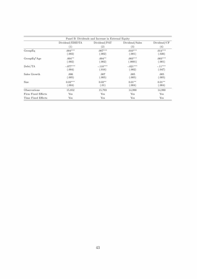
Panel B: Dividends and Increase in External Equity

Dividend/EBIDTA Dividend/PAT Dividend/Sales Dividend/CF

(1) (2) (3) (4)

GroupEq .004∗∗∗ .007∗∗∗ .010∗∗∗ .014∗∗∗(.002) (.002) (.001) (.026)

GroupEq*Age .004∗∗ .004∗∗ .003∗∗∗ .003∗∗∗(.002) (.002) (.0001) (.001)

Debt/TA -.077∗∗∗ -.110∗∗∗ -.021∗∗∗ -.11∗∗∗(.004) (.016) (.002) (.047)

Sales Growth .006 .007 .005 .005(.005) (.005) (.005) (.005)

Size 0.02∗∗∗ 0.02∗∗ 0.01∗∗ 0.01∗∗(.004) (.01) (.004) (.004)

Observations 15,852 15,793 14,990 14,990

Firm Fixed Effects Yes Yes Yes Yes

Time Fixed Effects Yes Yes Yes Yes

43

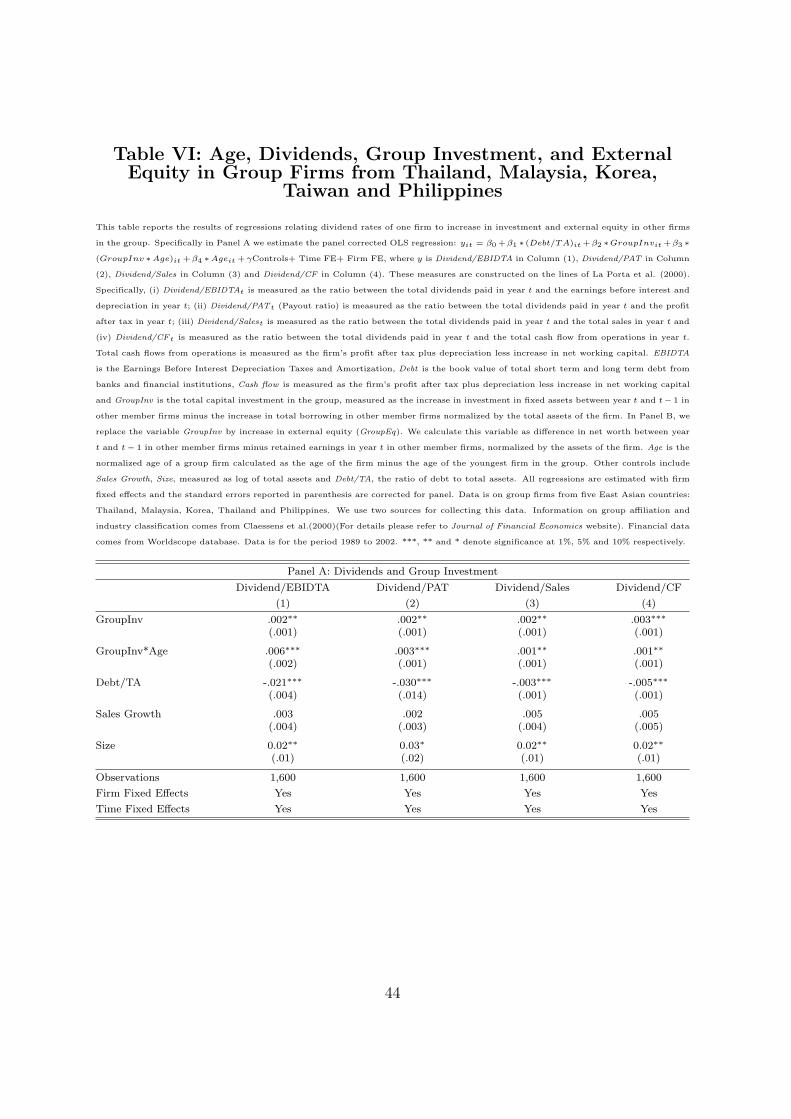
Table VI: Age, Dividends, Group Investment, and ExternalEquity in Group Firms from Thailand, Malaysia, Korea,

Taiwan and Philippines

This table reports the results of regressions relating dividend rates of one firm to increase in investment and external equity in other firms

in the group. Specifically in Panel A we estimate the panel corrected OLS regression: yit = β0 +β1 ∗ (Debt/TA)it +β2 ∗GroupInvit +β3 ∗(GroupInv ∗Age)it + β4 ∗Ageit + γControls+ Time FE+ Firm FE, where y is Dividend/EBIDTA in Column (1), Dividend/PAT in Column

(2), Dividend/Sales in Column (3) and Dividend/CF in Column (4). These measures are constructed on the lines of La Porta et al. (2000).

Specifically, (i) Dividend/EBIDTAt is measured as the ratio between the total dividends paid in year t and the earnings before interest and

depreciation in year t; (ii) Dividend/PATt (Payout ratio) is measured as the ratio between the total dividends paid in year t and the profit

after tax in year t; (iii) Dividend/Salest is measured as the ratio between the total dividends paid in year t and the total sales in year t and

(iv) Dividend/CFt is measured as the ratio between the total dividends paid in year t and the total cash flow from operations in year t.

Total cash flows from operations is measured as the firm’s profit after tax plus depreciation less increase in net working capital. EBIDTA

is the Earnings Before Interest Depreciation Taxes and Amortization, Debt is the book value of total short term and long term debt from

banks and financial institutions, Cash flow is measured as the firm’s profit after tax plus depreciation less increase in net working capital

and GroupInv is the total capital investment in the group, measured as the increase in investment in fixed assets between year t and t− 1 in

other member firms minus the increase in total borrowing in other member firms normalized by the total assets of the firm. In Panel B, we

replace the variable GroupInv by increase in external equity (GroupEq). We calculate this variable as difference in net worth between year

t and t− 1 in other member firms minus retained earnings in year t in other member firms, normalized by the assets of the firm. Age is the

normalized age of a group firm calculated as the age of the firm minus the age of the youngest firm in the group. Other controls include

Sales Growth, Size, measured as log of total assets and Debt/TA, the ratio of debt to total assets. All regressions are estimated with firm

fixed effects and the standard errors reported in parenthesis are corrected for panel. Data is on group firms from five East Asian countries:

Thailand, Malaysia, Korea, Thailand and Philippines. We use two sources for collecting this data. Information on group affiliation and

industry classification comes from Claessens et al.(2000)(For details please refer to Journal of Financial Economics website). Financial data

comes from Worldscope database. Data is for the period 1989 to 2002. ***, ** and * denote significance at 1%, 5% and 10% respectively.

Panel A: Dividends and Group Investment

Dividend/EBIDTA Dividend/PAT Dividend/Sales Dividend/CF

(1) (2) (3) (4)

GroupInv .002∗∗ .002∗∗ .002∗∗ .003∗∗∗(.001) (.001) (.001) (.001)

GroupInv*Age .006∗∗∗ .003∗∗∗ .001∗∗ .001∗∗(.002) (.001) (.001) (.001)

Debt/TA -.021∗∗∗ -.030∗∗∗ -.003∗∗∗ -.005∗∗∗(.004) (.014) (.001) (.001)

Sales Growth .003 .002 .005 .005(.004) (.003) (.004) (.005)

Size 0.02∗∗ 0.03∗ 0.02∗∗ 0.02∗∗(.01) (.02) (.01) (.01)

Observations 1,600 1,600 1,600 1,600

Firm Fixed Effects Yes Yes Yes Yes

Time Fixed Effects Yes Yes Yes Yes

44

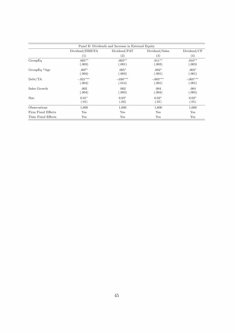
Panel B: Dividends and Increase in External Equity

Dividend/EBIDTA Dividend/PAT Dividend/Sales Dividend/CF

(1) (2) (3) (4)

GroupEq .005∗∗ .003∗∗ .011∗∗ .010∗∗(.003) (.001) (.003) (.003)

GroupEq *Age .007∗ .005∗ .002∗ .002∗(.004) (.003) (.001) (.001)

Debt/TA -.021∗∗∗ -.030∗∗∗ -.003∗∗∗ -.005∗∗∗(.004) (.014) (.001) (.001)

Sales Growth .002 .002 .004 .004(.004) (.003) (.004) (.005)

Size 0.01∗ 0.03∗ 0.02∗ 0.02∗(.01) (.02) (.01) (.01)

Observations 1,600 1,600 1,600 1,600

Firm Fixed Effects Yes Yes Yes Yes

Time Fixed Effects Yes Yes Yes Yes

45

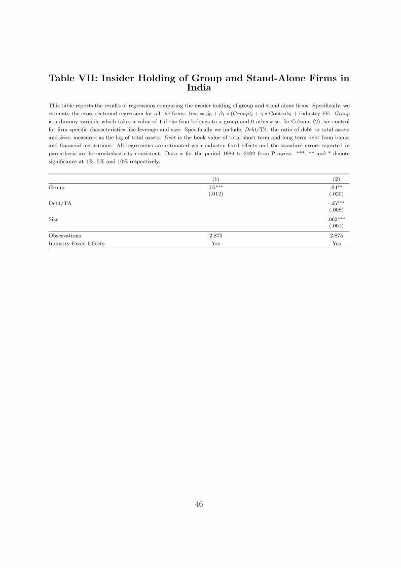
Table VII: Insider Holding of Group and Stand-Alone Firms inIndia

This table reports the results of regressions comparing the insider holding of group and stand alone firms. Specifically, we

estimate the cross-sectional regression for all the firms: Insi = β0 + β1 ∗ (Group)i + γ ∗ Controlsi + Industry FE. Group

is a dummy variable which takes a value of 1 if the firm belongs to a group and 0 otherwise. In Column (2), we control

for firm specific characteristics like leverage and size. Specifically we include, Debt/TA, the ratio of debt to total assets

and Size, measured as the log of total assets. Debt is the book value of total short term and long term debt from banks

and financial institutions. All regressions are estimated with industry fixed effects and the standard errors reported in

parenthesis are heteroskedasticity consistent. Data is for the period 1989 to 2002 from Prowess. ***, ** and * denote

significance at 1%, 5% and 10% respectively.

(1) (2)

Group .05∗∗∗ .04∗∗(.012) (.020)

Debt/TA -.45∗∗∗(.008)

Size .062∗∗∗(.001)

Observations 2,875 2,875

Industry Fixed Effects Yes Yes

46

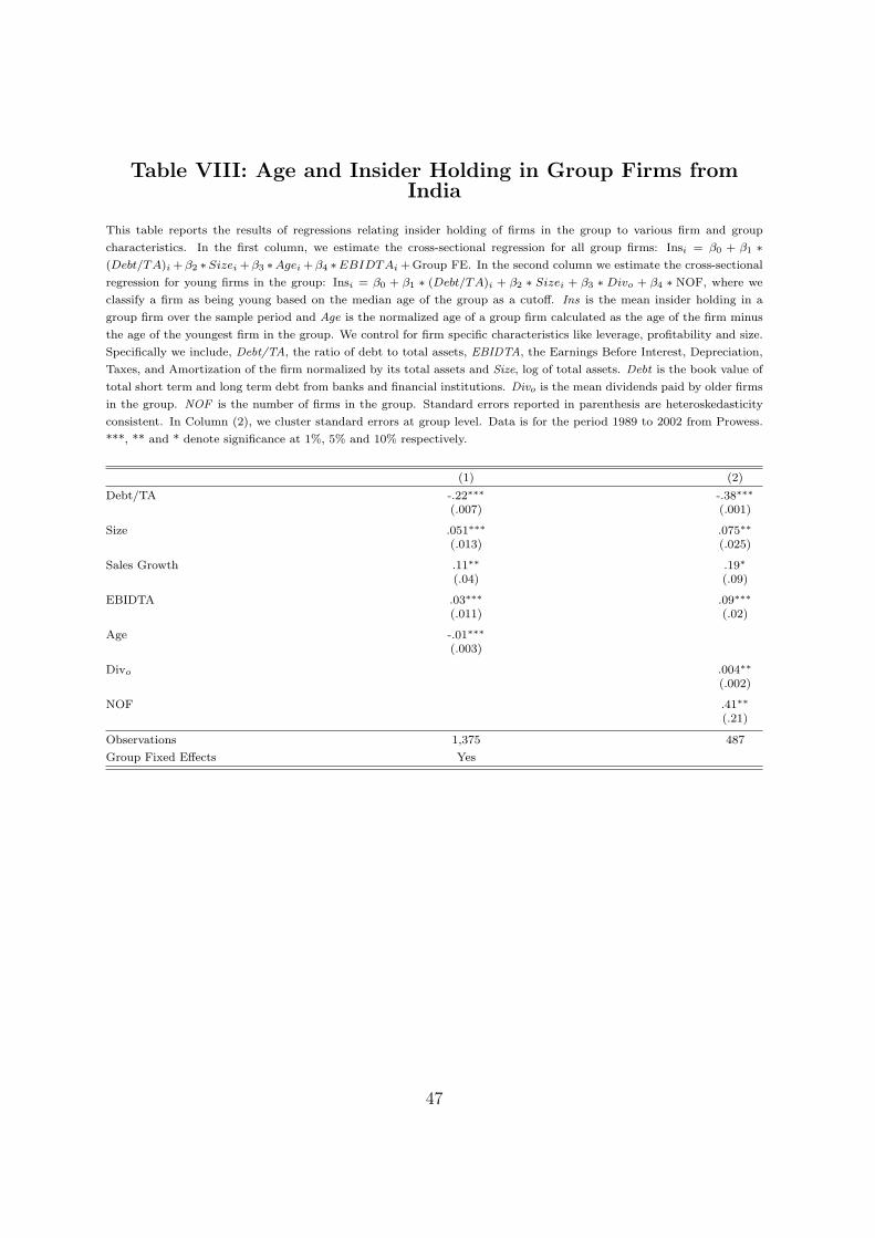
Table VIII: Age and Insider Holding in Group Firms fromIndia

This table reports the results of regressions relating insider holding of firms in the group to various firm and group

characteristics. In the first column, we estimate the cross-sectional regression for all group firms: Insi = β0 + β1 ∗(Debt/TA)i + β2 ∗Sizei + β3 ∗Agei + β4 ∗EBIDTAi + Group FE. In the second column we estimate the cross-sectional

regression for young firms in the group: Insi = β0 + β1 ∗ (Debt/TA)i + β2 ∗ Sizei + β3 ∗ Divo + β4 ∗ NOF, where we

classify a firm as being young based on the median age of the group as a cutoff. Ins is the mean insider holding in a

group firm over the sample period and Age is the normalized age of a group firm calculated as the age of the firm minus

the age of the youngest firm in the group. We control for firm specific characteristics like leverage, profitability and size.

Specifically we include, Debt/TA, the ratio of debt to total assets, EBIDTA, the Earnings Before Interest, Depreciation,

Taxes, and Amortization of the firm normalized by its total assets and Size, log of total assets. Debt is the book value of

total short term and long term debt from banks and financial institutions. Divo is the mean dividends paid by older firms

in the group. NOF is the number of firms in the group. Standard errors reported in parenthesis are heteroskedasticity

consistent. In Column (2), we cluster standard errors at group level. Data is for the period 1989 to 2002 from Prowess.

***, ** and * denote significance at 1%, 5% and 10% respectively.

(1) (2)

Debt/TA -.22∗∗∗ -.38∗∗∗(.007) (.001)

Size .051∗∗∗ .075∗∗(.013) (.025)

Sales Growth .11∗∗ .19∗(.04) (.09)

EBIDTA .03∗∗∗ .09∗∗∗(.011) (.02)

Age -.01∗∗∗(.003)

Divo .004∗∗(.002)

NOF .41∗∗(.21)

Observations 1,375 487

Group Fixed Effects Yes

47

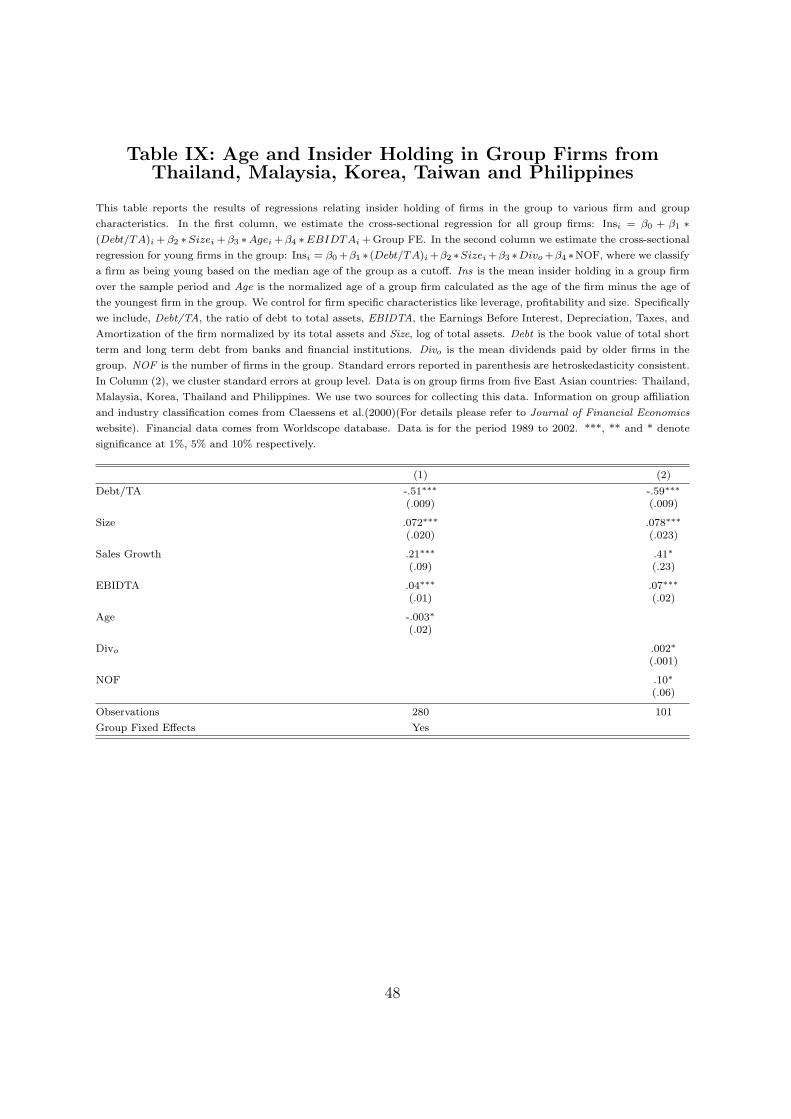
Table IX: Age and Insider Holding in Group Firms fromThailand, Malaysia, Korea, Taiwan and Philippines

This table reports the results of regressions relating insider holding of firms in the group to various firm and group

characteristics. In the first column, we estimate the cross-sectional regression for all group firms: Insi = β0 + β1 ∗(Debt/TA)i + β2 ∗Sizei + β3 ∗Agei + β4 ∗EBIDTAi + Group FE. In the second column we estimate the cross-sectional

regression for young firms in the group: Insi = β0 +β1 ∗ (Debt/TA)i +β2 ∗Sizei +β3 ∗Divo +β4 ∗NOF, where we classify

a firm as being young based on the median age of the group as a cutoff. Ins is the mean insider holding in a group firm

over the sample period and Age is the normalized age of a group firm calculated as the age of the firm minus the age of

the youngest firm in the group. We control for firm specific characteristics like leverage, profitability and size. Specifically

we include, Debt/TA, the ratio of debt to total assets, EBIDTA, the Earnings Before Interest, Depreciation, Taxes, and

Amortization of the firm normalized by its total assets and Size, log of total assets. Debt is the book value of total short

term and long term debt from banks and financial institutions. Divo is the mean dividends paid by older firms in the

group. NOF is the number of firms in the group. Standard errors reported in parenthesis are hetroskedasticity consistent.

In Column (2), we cluster standard errors at group level. Data is on group firms from five East Asian countries: Thailand,

Malaysia, Korea, Thailand and Philippines. We use two sources for collecting this data. Information on group affiliation

and industry classification comes from Claessens et al.(2000)(For details please refer to Journal of Financial Economics

website). Financial data comes from Worldscope database. Data is for the period 1989 to 2002. ***, ** and * denote

significance at 1%, 5% and 10% respectively.

(1) (2)

Debt/TA -.51∗∗∗ -.59∗∗∗(.009) (.009)

Size .072∗∗∗ .078∗∗∗(.020) (.023)

Sales Growth .21∗∗∗ .41∗(.09) (.23)

EBIDTA .04∗∗∗ .07∗∗∗(.01) (.02)

Age -.003∗(.02)

Divo .002∗(.001)

NOF .10∗(.06)

Observations 280 101

Group Fixed Effects Yes

48