Google’s MapReduce programming model — …€™s MapReduce programming model — Revisited Ralf...

Science of Computer Programming 70 (2008) 1–30www.elsevier.com/locate/scico

Google’s MapReduce programming model — Revisited

Ralf Lammel∗

Data Programmability Team, Microsoft Corp., Redmond, WA, USA

Received 9 February 2006; received in revised form 10 July 2007; accepted 10 July 2007Available online 18 July 2007

Abstract

Google’s MapReduce programming model serves for processing large data sets in a massively parallel manner. We deliverthe first rigorous description of the model including its advancement as Google’s domain-specific language Sawzall. To this end,we reverse-engineer the seminal papers on MapReduce and Sawzall, and we capture our findings as an executable specification.We also identify and resolve some obscurities in the informal presentation given in the seminal papers. We use typed functionalprogramming (specifically Haskell) as a tool for design recovery and executable specification. Our development comprises threecomponents: (i) the basic program skeleton that underlies MapReduce computations; (ii) the opportunities for parallelism inexecuting MapReduce computations; (iii) the fundamental characteristics of Sawzall’s aggregators as an advancement of theMapReduce approach. Our development does not formalize the more implementational aspects of an actual, distributed executionof MapReduce computations.c© 2007 Elsevier B.V. All rights reserved.

Keywords: Data processing; Parallel programming; Distributed programming; Software design; Executable specification; Typed functionalprogramming; MapReduce; Sawzall; Map; Reduce; List homomorphism; Haskell

1. Introduction

Google’s MapReduce programming model [10] serves for processing large data sets in a massively parallel manner(subject to a ‘MapReduce implementation’).1 The programming model is based on the following, simple concepts: (i)iteration over the input; (ii) computation of key/value pairs from each piece of input; (iii) grouping of all intermediatevalues by key; (iv) iteration over the resulting groups; (v) reduction of each group. For instance, consider a repositoryof documents from a web crawl as input, and a word-based index for web search as output, where the intermediatekey/value pairs are of the form 〈word,URL〉.

The model is stunningly simple, and it effectively supports parallelism. The programmer may abstract from theissues of distributed and parallel programming because it is the MapReduce implementation that takes care of loadbalancing, network performance, fault tolerance, etc. The seminal MapReduce paper [10] described one possibleimplementation model based on large networked clusters of commodity machines with local store. The programmingmodel may appear as restrictive, but it provides a good fit for many problems encountered in the practice of processing

∗ Corresponding address: Universitat Koblenz-Landau, Institut fur Informatik B 128, Universitatsstrasse 1, D-56070 Koblenz, Germany.E-mail address: [email protected].

1 Also see: http://en.wikipedia.org/wiki/MapReduce.

0167-6423/$ - see front matter c© 2007 Elsevier B.V. All rights reserved.doi:10.1016/j.scico.2007.07.001

http://www.elsevier.com/locate/scico

mailto:[email protected]

http://en.wikipedia.org/wiki/MapReduce






http://dx.doi.org/10.1016/j.scico.2007.07.001

2 R. Lammel / Science of Computer Programming 70 (2008) 1–30

large data sets. Also, expressiveness limitations may be alleviated by decomposition of problems into multipleMapReduce computations, or by escaping to other (less restrictive, but more demanding) programming models forsubproblems.

In the present paper, we deliver the first rigorous description of the model including its advancement as Google’sdomain-specific language Sawzall [26]. To this end, we reverse-engineer the seminal MapReduce and Sawzall papers,and we capture our findings as an executable specification. We also identify and resolve some obscurities in theinformal presentation given in the seminal papers. Our development comprises three components: (i) the basic programskeleton that underlies MapReduce computations; (ii) the opportunities for parallelism in executing MapReducecomputations; (iii) the fundamental characteristics of Sawzall’s aggregators as an advancement of the MapReduceapproach. Our development does not formalize the more implementational aspects of an actual, distributed executionof MapReduce computations (i.e., aspects such as fault tolerance, storage in a distributed file system, and taskscheduling).

Our development uses typed functional programming, specifically Haskell, as a tool for design recovery andexecutable specification. (We tend to restrict ourselves to Haskell 98 [24], and point out deviations.) As a byproduct,we make another case for the utility of typed functional programming as part of a semi-formal design methodology.The use of Haskell is augmented by explanations targeted at readers without proficiency in Haskell and functionalprogramming. Some cursory background in declarative programming and typed programming languages is assumed,though.

The paper is organized as follows. Section 2 recalls the basics of the MapReduce programming model and thecorresponding functional programming combinators. Section 3 develops a baseline specification for MapReducecomputations with a typed, higher-order function capturing the key abstraction for such computations. Section 4 coversparallelism and distribution. Section 5 studies Sawzall’s aggregators in relation to the MapReduce programmingmodel. Section 6 concludes the paper.

2. Basics of map and reduce

We will briefly recapitulate the MapReduce programming model. We quote: the MapReduce “abstraction isinspired by the map and reduce primitives present in Lisp and many other functional languages” [10]. Therefore, wewill also recapitulate the relevant list-processing combinators, map and reduce, known from functional programming.We aim to get three levels right: (i) higher-order combinators for mapping and reduction vs. (ii) the principledarguments of these combinators vs. (iii) the actual applications of the former to the latter. (These levels are somewhatconfused in the seminal MapReduce paper.)

2.1. The MapReduce programming model

The MapReduce programming model is clearly summarized in the following quote [10]:

“The computation takes a set of input key/value pairs, and produces a set of output key/value pairs. The user ofthe MapReduce library expresses the computation as two functions: map and reduce.

Map, written by the user, takes an input pair and produces a set of intermediate key/value pairs. TheMapReduce library groups together all intermediate values associated with the same intermediate key I andpasses them to the reduce function.

The reduce function, also written by the user, accepts an intermediate key I and a set of values for that key.It merges together these values to form a possibly smaller set of values. Typically just zero or one output valueis produced per reduce invocation. The intermediate values are supplied to the user’s reduce function via aniterator. This allows us to handle lists of values that are too large to fit in memory.”

We also quote an example including pseudo-code [10]:

“Consider the problem of counting the number of occurrences of each word in a large collection of documents.The user would write code similar to the following pseudo-code:

R. Lammel / Science of Computer Programming 70 (2008) 1–30 3

map(String key, String value): reduce(String key, Iterator values):// key: document name // key: a word// value: document contents // values: a list of countsfor each word w in value: int result = 0;EmitIntermediate(w, "1"); for each v in values:

result += ParseInt(v);Emit(AsString(result));

The map function emits each word plus an associated count of occurrences (just ‘1’ in this simple example). Thereduce function sums together all counts emitted for a particular word.”

2.2. Lisp’s map and reduce

Functional programming stands out when designs can benefit from the employment of recursion schemes for listprocessing, and more generally data processing. Recursion schemes like map and reduce enable powerful formsof decomposition and reuse. Quite to the point, the schemes directly suggest parallel execution, say expressionevaluation — if the problem-specific ingredients are free of side effects and meet certain algebraic properties. Giventhe quoted reference to Lisp, let us recall the map and reduce combinators of Lisp. The following two quotes stemfrom “Common Lisp, the Language” [30]2:

map result-type function sequence &rest more-sequences

“The function must take as many arguments as there are sequences provided; at least one sequence must be provided.The result of map is a sequence such that element j is the result of applying function to element j of each of the argumentsequences. The result sequence is as long as the shortest of the input sequences.”

This kind of map combinator is known to compromise on orthogonality. That is, mapping over a single list issufficient — if we assume a separate notion of ‘zipping’ such that n lists are zipped together to a single list ofn-tuples.

reduce function sequence &key :from-end :start :end :initial-value

“The reduce function combines all the elements of a sequence using a binary operation; for example, using + one can addup all the elements.

The specified subsequence of the sequence is combined or “reduced” using the function, which must accept twoarguments. The reduction is left-associative, unless the :from-end argument is true (it defaults to nil), in which caseit is right-associative. If an :initial-value argument is given, it is logically placed before the subsequence (after it if:from-end is true) and included in the reduction operation.

If the specified subsequence contains exactly one element and the keyword argument :initial-value is not given,then that element is returned and the function is not called. If the specified subsequence is empty and an :initial-value is given, then the :initial-value is returned and the function is not called.

If the specified subsequence is empty and no :initial-value is given, then the function is called with zeroarguments, and reduce returns whatever the function does. (This is the only case where the function is called with otherthan two arguments.)”

(We should note that this is not yet the most general definition of reduction in Common Lisp.) It is common to assumethat function is free of side effects, and it is an associative (binary) operation with :initial-value as its unit.In the remainder of the paper, we will be using the term ‘proper reduction’ in such a case.

2.3. Haskell’s map and reduce

The Haskell standard library (in fact, the so-called ‘prelude’) defines related combinators. Haskell’s mapcombinator processes a single list as opposed to Lisp’s combinator for an arbitrary number of lists. The kind ofleft-associative reduction of Lisp is provided by Haskell’s foldl combinator — except that the type of foldl is moregeneral than necessary for reduction. We attach some Haskell illustrations that can be safely skipped by the readerwith proficiency in typed functional programming.

2 At the time of writing, the relevant quotes are available online: http://www.cs.cmu.edu/Groups/AI/html/cltl/clm/node143.html.

http://www.cs.cmu.edu/Groups/AI/html/cltl/clm/node143.html













Illustration of map: Let us double all numbers in a list:

Haskell-prompt> map ((∗) 2) [1,2,3][2,4,6]

Here, the expression ‘ ((∗) 2) ’ denotes multiplication by 2.

In (Haskell’s) lambda notation, ‘ ((∗) 2) ’ can also be rendered as ‘\x −> 2∗x’.

Illustration of foldl: Let us compute the sum of all numbers in a list:

Haskell-prompt> foldl (+) 0 [1,2,3]6

Here, the expression ‘(+)’ denotes addition and the constant ‘0’ is the default value. The left-associative bias of foldlshould be apparent from the parenthesization in the following evaluation sequence:

foldl (+) 0 [1,2,3]⇒ (((0 + 1) + 2) + 3)⇒ 6

Definition of map

map :: (a −> b) −> [a] −> [b] −− type of mapmap f [] = [] −− equation: the empty list casemap f (x:xs) = f x : map f xs −− equation: the non−empty list case

The (polymorphic) type of the map combinator states that it takes two arguments: a function of type a −> b, and alist of type [a]. The result of mapping is a list of type [b]. The type variables a and b correspond to the element typesof the argument and result lists. The first equation states that mapping f over an empty list (denoted as [] ) returns theempty list. The second equation states that mapping f over a non-empty list, x:xs, returns a list whose head is f appliedto x, and whose tail is obtained by recursively mapping over xs.

Haskell trivia

• Line comments start with ‘−−’.• Function names start in lower case; cf. map and foldl .• In types, ’...−>...’ denotes the type constructor for function types.• In types, ’ [...] ’ denotes the type constructor for lists.• Term variables start in lower case; cf. x and xs.• Type variables start in lower case, too; cf. a and b.• Type variables are implicitly universally quantified, but can be explicitly universally quantified. For instance, the type of map

changes as follows, when using explicit quantification: map :: forall a b . ( a −> b) −> [a] −> [b]• Terms of a list type can be of two forms:

– The empty list: ’ [] ’– The non-empty list consisting of head and tail: ’... : ...’

3

Definition of foldl

foldl :: ( b −> a −> b) −> b −> [a] −> b −− type of foldlfoldl f y [] = y −− equation: the empty list casefoldl f y (x:xs) = foldl f ( f y x ) xs −− equation: the non−empty list case

The type of the foldl combinator states that it takes three arguments: a binary operation of type b −> a −> b, a‘default value’ of type b and a list of type [a] to fold over. The result of folding is of type b. The first equation statesthat an empty list is mapped to the default value. The second equation states that folding over a non-empty list requiresrecursion into the tail and application of the binary operation f to the folding result so far and the head of the list. Wecan restrict foldl to what is normally called reduction by type specialization:

reduce :: ( a −> a −> a) −> a −> [a] −> areduce = foldl


Asides on folding

• For the record, we mention that the combinators map and foldl can actually be both defined in terms of the right-associative fold operation, foldr , [23,20]. Hence, foldr can be considered as the fundamental recursion schemefor list traversal. The functions that are expressible in terms of foldr are also known as ‘list catamorphisms’ or‘bananas’. We include the definition of foldr for completeness’ sake:

foldr :: ( a −> b −> b) −> b −> [a] −> b −− type of foldrfoldr f y [] = y −− equation: the empty list casefoldr f y (x:xs) = f x ( foldr f y xs) −− equation: the non−empty list case

• Haskell’s lazy semantics makes applications of foldl potentially inefficient due to unevaluated chunks ofintermediate function applications. Hence, it is typically advisable to use a strict companion or the right-associativefold operator, foldr , but we neglect such details of Haskell in the present paper.• Despite left-associative reduction as Lisp’s default, one could also take the position that reduction should be right-

associative. We follow Lisp for now and reconsider in Section 5, where we notice that monoidal reduction inHaskell is typically defined in terms of foldr — the right-associative fold combinator.

2.4. MapReduce’s map & reduce

Here is the obvious question. How do MapReduce’s map and reduce correspond to standard map and reduce? Forclarity, we use a designated font for MapReduce’s MAP and REDUCE , from here on. The following overview listsmore detailed questions and summarizes our findings:

Question FindingIsMAP essentially the map combinator? NOIsMAP essentially an application of the map combinator? NODoesMAP essentially serve as the argument of map? YESIsREDUCE essentially the reduce combinator? NOIsREDUCE essentially an application of the reduce combinator? TYPICALLYDoesREDUCE essentially serve as the argument of reduce? NODoesREDUCE essentially serve as the argument of map? YES

Hence, there is no trivial correspondence between MapReduce’s MAP & REDUCE and what is normally calledmap & reduce in functional programming. Also, the relationships between MAP and map are different from thosebetween REDUCE and reduce. For clarification, let us consider again the sample code for the problem of countingoccurrences of words:

map(String key, String value): reduce(String key, Iterator values):// key: document name // key: a word// value: document contents // values: a list of countsfor each word w in value: int result = 0;EmitIntermediate(w, "1"); for each v in values:

result += ParseInt(v);Emit(AsString(result));

Per programming model, both functions are applied to key/value pairs one-by-one. Naturally, our executablespecification will use the standard map combinator to apply MAP and REDUCE to all input or intermediate data.Let us now focus on the inner workings of MAP and REDUCE .

Internals of REDUCE: The situation is straightforward at first sight. The above code performs imperativeaggregation (say, reduction): take many values, and reduce them to a single value. This seems to be the case formost MapReduce examples that are listed in [10]. Hence, MapReduce’s REDUCE typically performs reduction, i.e.,it can be seen as an application of the standard reduce combinator.

However, it is important to notice that the MapReduce programmer is not encouraged to identify the ingredientsof reduction, i.e., an associative operation with its unit. Also, the assigned type of REDUCE , just by itself, is slightlydifferent from the type to be expected for reduction, as we will clarify in the next section. Both deviations from thefunctional programming letter may have been chosen by the MapReduce designers for reasons of flexibility. Here isactually one example from the MapReduce paper that goes beyond reduction in a narrow sense [10]:


“Inverted index: The map function parses each document, and emits a sequence of 〈word,document ID〉 pairs.The reduce function accepts all pairs for a given word, sorts the corresponding document IDs and emits a 〈word,list(document ID)〉 pair.”

In this example,REDUCE performs sorting as opposed to the reduction of many values to one. The MapReduce paperalso alludes to filtering in another case. We could attempt to provide a more general characterization for REDUCE .Indeed, our Sawzall investigation in Section 5 will lead to an appropriate generalization.

Internals ofMAP: We had already settled thatMAP is mapped over key/value pairs (just as much asREDUCE).So it remains to poke at the internal structure ofMAP to see whether there is additional justification forMAP to berelated to mapping (other than the sort of mapping that also applies to REDUCE). In the above sample code, MAPsplits up the input value into words; alike for the ‘inverted index’ example that we quoted. Hence, MAP seems toproduce lists, it does not seem to traverse lists, say consume lists. In different terms,MAP is meant to associate eachgiven key/value pair of the input with potentially many intermediate key/value pairs. For the record, we mention thatthe typical kind of MAP function could be characterized as an instance of unfolding (also known as anamorphismsor lenses [23,16,1]).3

3. The MapReduce abstraction

We will now enter reverse-engineering mode with the goal to extract an executable specification (in fact, a relativelysimple Haskell function) that captures the abstraction for MapReduce computations. An intended byproduct is thedetailed demonstration of Haskell as a tool for design recovery and executable specification.

3.1. The power of ‘.’

Let us discover the main blocks of a function mapReduce, which is assumed to model the abstraction forMapReduce computations. We recall that MAP is mapped over the key/value pairs of the input, while REDUCE ismapped over suitably grouped intermediate data. Grouping takes place in between the map and reduce phases [10]:“The MapReduce library groups together all intermediate values associated with the same intermediate key I andpasses them to the reduce function”. Hence, we take for granted that mapReduce can be decomposed as follows:

mapReduce mAP rEDUCE= reducePerKey −− 3. Apply REDUCE to each group. groupByKey −− 2. Group intermediate data per key. mapPerKey −− 1. Apply MAP to each key / value pair

wheremapPerKey = ⊥ −− to be discoveredgroupByKey = ⊥ −− to be discoveredreducePerKey = ⊥ −− to be discovered

Here, the arguments mAP and rEDUCE are placeholders for the problem-specific functions MAP and REDUCE .The function mapReduce is the straight function composition over locally defined helper functions mapPerKey,groupByKey and reducePerKey, which we leave undefined — until further notice.

We defined the mapReduce function in terms of function composition, which is denoted by Haskell’s infix operator‘.’. (The dot ‘applies from right to left’, i.e., (g . f ) x = g ( f x).) The systematic use of function compositionimproves clarity. That is, the definition of the mapReduce function expresses very clearly that a MapReducecomputation is composed from three phases.

3 The source-code distribution illustrates the use of unfolding (for the words function) in the map phase; cf. module Misc.Unfold.


More Haskell trivia: For comparison, we also illustrate other styles of composing together the mapReduce function from thethree components. Here is a transcription that uses Haskell’s plain function application:

mapReduce mAP rEDUCE input =reducePerKey (groupByKey (mapPerKey input))

where ...

Function application, when compared to function composition, slightly conceals the fact that a MapReduce computation iscomposed from three phases. Haskell’s plain function application, as exercised above, is left-associative and relies on juxtaposition(i.e., putting function and argument simply next to each other). There is also an explicit operator, ‘$’ for right-associative functionapplication, which may help reducing parenthesization. For instance, ‘ f $ x y’ denotes ‘ f ( x y)’. Here is another version of themapReduce function:

mapReduce mAP rEDUCE input =reducePerKey

$ groupByKey$ mapPerKey input

where ...

3

For the record, the systematic use of function combinators like ‘ .’ leads to ‘point-free’ style [3,14,15]. The term‘point’ refers to explicit arguments, such as input in the illustrative code snippets, listed above. That is, a point-freedefinition basically only uses function combinators but captures no arguments explicitly. Backus, in his Turing Awardlecture in 1978, also uses the term ‘functional forms’ [2].

3.2. The undefinedness idiom

In the first draft of the mapReduce function, we left all components undefined. (The textual representationfor Haskell’s ‘⊥’ (say, bottom) is ‘undefined’.) Generally. ‘⊥’ is an extremely helpful instrument in specificationdevelopment. By leaving functions ‘undefined’, we can defer discovering their types and definitions until later. Ofcourse, we cannot evaluate an undefined expression in any useful way:

Haskell-prompt> undefined∗∗∗ Exception: Prelude.undefined

Taking into account laziness, we may evaluate partial specifications as long as we are not ‘strict’ in (say, dependent on)undefined parts. More importantly, a partial specification can be type-checked. Hence, the ‘undefinedness’ idiom canbe said to support top–down steps in design. The convenient property of ‘⊥’ is that it has an extremely polymorphictype:

Haskell-prompt> : t undefinedundefined :: a

Hence, ‘⊥’ may be used virtually everywhere. Functions that are undefined (i.e., whose definition equals ‘⊥’) areequally polymorphic and trivially participate in type inference and checking. One should compare such expressivenesswith the situation in state-of-the-art OO languages such as C# 3.0 or Java 1.6. That is, in these languages, methodsmust be associated with explicitly declared signatures, despite all progress with type inference. The effectiveness ofHaskell’s ‘undefinedness’ idiom relies on full type inference so that ‘⊥’ can be used freely without requiring anyannotations for types that are still to be discovered.

3.3. Type discovery from prose

The type of the scheme for MapReduce computations needs to be discovered. (It is not defined in the MapReducepaper.) We can leverage the types for MAP and REDUCE , which are defined as follows [10]:

“Conceptually the map and reduce functions [...] have associated types:

map (k1,v1) −> list(k2,v2)reduce (k2, list (v2)) −> list (v2)


I.e., the input keys and values are drawn from a different domain than the output keys and values. Furthermore,the intermediate keys and values are from the same domain as the output keys and values.”

The above types are easily expressed in Haskell — except that we must be careful to note that the following functionsignatures are somewhat informal because of the way we assume sharing among type variables of function signatures.

map :: k1 −> v1 −> [(k2,v2)]reduce :: k2 −> [v2] −> [v2]

(Again, our reuse of the type variables k2 and v2 should be viewed as an informal hint.) The type of a MapReducecomputation was informally described as follows [10]: “the computation takes a set of input key/value pairs, andproduces a set of output key/value pairs”. We will later discuss the tension between ‘list’ (in the earlier types) and‘set’ (in the wording). For now, we just continue to use ‘list’, as suggested by the above types. So let us turn prose intoa Haskell type:

computation :: [( k1,v1)] −> [(k2,v2)]

Hence, the following type is implied for mapReduce:

−− To be amended!mapReduce :: (k1 −> v1 −> [(k2,v2)]) −− TheMAP function

−> (k2 −> [v2] −> [v2]) −− TheREDUCE function−> [( k1,v1 )] −− A set of input key / value pairs−> [( k2,v2 )] −− A set of output key / value pairs

Haskell sanity-checks this type for us, but this type is not the intended one. An application of REDUCE is said toreturn a list (say, a group) of output values per output key. In contrast, the result of a MapReduce computation is aplain list of key/value pairs. This may mean that the grouping of values per key has been (accidentally) lost. (We notethat this difference only matters if we are not talking about the ‘typical case’ of zero or one value per key.) We proposethe following amendment:

mapReduce :: (k1 −> v1 −> [(k2,v2)]) −− TheMAP function−> (k2 −> [v2] −> [v2]) −− TheREDUCE function−> [( k1,v1 )] −− A set of input key / value pairs−> [( k2,[v2] )] −− A set of output key / value− list pairs

The development illustrates that types greatly help in capturing and communicating designs (in addition to plain prosewith its higher chances of imprecision). Clearly, for types to serve this purpose effectively, we are in need of a typelanguage that is powerful (so that types carry interesting information) as well as readable and succinct.

3.4. Type-driven reflection on designs

The readability and succinctness of types is also essential for making them useful in reflection on designs. In fact,how would we somehow systematically reflect on designs other than based on types? Design patterns [12] may cometo mind. However, we contend that their actual utility for the problem at hand is non-obvious, but one may argue thatwe are in the process of discovering a design pattern, and we inform our proposal in a type-driven manner.

The so-far proposed type of mapReduce may trigger the following questions:

• Why do we need to require a list type for output values?• Why do the types of output and intermediate values coincide?• When do we need lists of key/value pairs, or sets, or something else?

These questions may pinpoint potential over-specifications.


Why do we need to require a list type for output values?Let us recall that the programming model was described such that “typically just zero or one output value is

produced per reduce invocation” [10]. We need a type for REDUCE such that we cover the ‘general case’, but let usbriefly look at a type for the ‘typical case’:

mapReduce :: (k1 −> v1 −> [(k2,v2)]) −− TheMAP function−> (k2 −> [v2] −> Maybe v2) −− TheREDUCE function−> [( k1,v1 )] −− A set of input key / value pairs−> [( k2,v2 )] −− A set of output key / value pairs

The use of Maybe allows the REDUCE function to express that “zero or one” output value is returned for the givenintermediate values. Further, we assume that a key with the associated reduction result Nothing should not contributeto the final list of key/value pairs. Hence, we omit Maybe in the result type of mapReduce.

More Haskell trivia: We use the Maybe type constructor to model optional values. Values of this type can be constructed intwo ways. The presence of a value v is denoted by a term of the form ‘Just v’, whereas the absence of any value is denoted by‘Nothing’. For completeness’ sake, here is the declaration of the parametric data type Maybe:

data Maybe v = Just v | Nothing

3

Why do the types of output and intermediate values coincide?Reduction is normally understood to take many values and to return a single value (of the same type as the element

type for the input). However, we recall that some MapReduce scenarios go beyond this typing scheme; recall sortingand filtering. Hence, let us experiment with the distinction of two types:

• v2 for intermediate values;• v3 for output values.

The generalized type for the typical case looks as follows:

mapReduce :: (k1 −> v1 −> [(k2,v2)]) −− TheMAP function−> (k2 −> [v2] −> Maybe v3) −− TheREDUCE function−> [( k1,v1 )] −− A set of input key / value pairs−> [( k2,v3 )] −− A set of output key / value pairs

It turns out that we can re-enable the original option of multiple reduction results by instantiating v3 to a list type. Forbetter assessment of the situation, let us consider a list of options for REDUCE’s type:

• k2 −> [v2] −> [v2] (The original type from the MapReduce paper)• k2 −> [v2] −> v2 (The type for Haskell/Lisp-like reduction)• k2 −> [v2] −> v3 (With a type distinction as in folding)• k2 −> [v2] −> Maybe v2 (The typical MapReduce case)• k2 −> [v2] −> Maybe v3 (The proposed generalization)

We may instantiate v3 as follows:

• v3 7→ v2 We obtain the aforementioned typical case.• v3 7→ [v2] We obtain the original type — almost.

The generalized type admits two ‘empty’ values: Nothing and Just [] . This slightly more complicated situation allowsfor more precision. That is, we do not need to assume an overloaded interpretation of the empty list to imply theomission of a corresponding key/value pair in the output.


When do we need lists of key/value pairs, or sets, or something else?Let us reconsider the sloppy use of lists or sets of key/value pairs in some prose we had quoted. We want to

modify mapReduce’s type one more time to gain in precision of typing. It is clear that saying ‘lists of key/value pairs’does neither imply mutually distinct pairs nor mutually distinct keys. Likewise, saying ‘sets of key/value pairs’ onlyrules out the same key/value pair to be present multiple times. We contend that a stronger data invariant is neededat times — the one of a dictionary type (say, the type of an association map or a finite map). We revise the type ofmapReduce one more time, while we leverage an abstract data type, Data.Map.Map, for dictionaries:

import Data.Map −− Library for dictionaries

mapReduce :: (k1 −> v1 −> [(k2,v2)]) −− TheMAP function−> (k2 −> [v2] −> Maybe v3) −− TheREDUCE function−> Map k1 v1 −− A key to input−value mapping−> Map k2 v3 −− A key to output−value mapping

It is important to note that we keep using the list-type constructor in the result position for the type of MAP .Prose [10] tells us that MAP “produces a set of intermediate key/value pairs”, but, this time, it is clear that listsof intermediate key/value pairs are meant. (Think of the running example where many pairs with the same word mayappear, and they all should count.)

Haskell’s dictionary type: We will be using the following operations on dictionaries:

• toList — export dictionary as list of pairs.• fromList — construct dictionary from list of pairs.• empty — construct the empty dictionary.• insert — insert key/value pair into dictionary.• mapWithKey — list-like map over a dictionary: this operation operates on the key/value pairs of a dictionary (as opposed to

lists of arbitrary values). Mapping preserves the key of each pair.• filterWithKey — filter dictionary according to predicate: this operation is essentially the standard filter operation for lists,

except that it operates on the key/value pairs of a dictionary. That is, the operation takes a predicate that determines allelements (key/value pairs) to remain in the dictionary.• insertWith — insert with aggregating value domain: Consider an expression of the form ‘insertWith o k v dict’. The result of

its evaluation is defined as follows. If dict does not hold any entry for the key k, then dict is extended by an entry that mapsthe key k to the value v. If dict readily maps the key k to a value v′, then this entry is updated with a combined value, which isobtained by applying the binary operation o to v′ and v.• unionsWith — combine dictionaries with aggregating value domain.

3

The development illustrates that types may be effectively used to discover, identify and capture invariants and variationpoints in designs. Also, the development illustrates that type-level reflection on a problem may naturally triggergeneralizations that simplify or normalize designs.

3.5. Discovery of types

We are now in the position to discover the types of the helper functions mapPerKey, groupByKey and reducePerKey.While there is no rule that says ‘discover types first, discover definitions second’, this order is convenient in thesituation at hand.

We should clarify that Haskell’s type inference does not give us useful types for mapPerKey and the other helperfunctions. The problem is that these functions are undefined, hence they carry the uninterestingly polymorphic typeof ‘⊥’. We need to take into account problem-specific knowledge and the existing uses of the undefined functions.

We start from the ‘back’ of mapReduce’s function definition — knowing that we can propagate the input type ofmapReduce through the function composition. For ease of reference, we inline the definition of mapReduce again:

mapReduce mAP rEDUCE = reducePerKey . groupByKey . mapPerKey where ...

The function mapPerKey takes the input of mapReduce, which is of a known type.Hence, we can sketch the type of mapPerKey so far:


... wheremapPerKey :: Map k1 v1 −− A key to input−value mapping

−> ? ? ? −− What’s the result and its type?

More Haskell trivia: We must note that our specification relies on a Haskell 98 extension for lexically scoped type variables [25].This extension allows us to reuse type variables from the signature of the top-level function mapReduce in the signatures of localhelpers such as mapPerKey.4

3

The discovery of mapPerKey’s result type requires domain knowledge. We know that mapPerKey maps MAP overthe input; the type ofMAP tells us the result type for each element in the input: a list of intermediate key/value pairs.We contend that the full map phase over the entire input should return the same kind of list (as opposed to a nestedlist). Thus:

... wheremapPerKey :: Map k1 v1 −− A key to input−value mapping

−> [( k2,v2 )] −− The intermediate key / value pairs

The result type of mapPerKey provides the argument type for groupByKey. We also know that groupByKey “groupstogether all intermediate values associated with the same intermediate key”, which suggests a dictionary type for theresult. Thus:

... wheregroupByKey :: [( k2,v2 )] −− The intermediate key / value pairs

−> Map k2 [v2] −− The grouped intermediate values

The type of reducePerKey is now sufficiently constrained by its position in the chained function composition:its argument type coincides with the result type of groupByKey; its result type coincides with the result type ofmapReduce. Thus:

... wherereducePerKey :: Map k2 [v2] −− The grouped intermediate values

−> Map k2 v3 −− A key to output−value mapping

Starting from types or definitions: We have illustrated the use of ‘starting from types’ as opposed to ‘starting fromdefinitions’ or any mix in between. When we start from types, an interesting (non-trivial) type may eventually suggestuseful ways of populating the type. In contrast, when we start from definitions, less interesting or more complicatedtypes may eventually be inferred from the (more interesting or less complicated) definitions. As an aside, one maycompare the ‘start from definitions vs. types’ scale with another well-established design scale for software: top–downor bottom–up or mixed mode.

3.6. Discovery of definitions

It remains to define mapPerKey, groupByKey and reducePerKey. The discovered types for these helpers are quitetelling; we contend that the intended definitions could be found semi-automatically, if we were using an ‘informed’type-driven search algorithm for expressions that populate a given type. We hope to prove this hypothesis some day.For now, we discover the definitions in a manual fashion. As a preview, and for ease of reference, the completemapReduce function is summarized in Fig. 1.

4 The source-code distribution for this paper also contains a pure Haskell 98 solution where we engage in encoding efforts such that we use anauxiliary record type for imposing appropriately polymorphic types on mapReduce and all its ingredients; cf. module MapReduce.Haskell98.


module MapReduce.Basic ( mapReduce) where

import Data.Map (Map,empty,insertWith,mapWithKey,filterWithKey,toList)

mapReduce :: forall k1 k2 v1 v2 v3.Ord k2 −− Needed for grouping

=> (k1 −> v1 −> [(k2,v2)]) −− TheMAP function−> (k2 −> [v2] −> Maybe v3) −− TheREDUCE function−> Map k1 v1 −− A key to input−value mapping−> Map k2 v3 −− A key to output−value mapping

mapReduce mAP rEDUCE =reducePerKey −− 3. Apply REDUCE to each group

. groupByKey −− 2. Group intermediate data per key

. mapPerKey −− 1. Apply MAP to each key / value pair

wheremapPerKey :: Map k1 v1 −> [(k2,v2)]mapPerKey =

concat −− 3. Concatenate per−key lists. map (uncurry mAP) −− 2. MapMAP over list of pairs. toList −− 1. Turn dictionary into list

groupByKey :: [(k2,v2)] −> Map k2 [v2]groupByKey = foldl insert empty

whereinsert dict ( k2,v2) = insertWith (++) k2 [v2] dict

reducePerKey :: Map k2 [v2] −> Map k2 v3reducePerKey =

mapWithKey unJust −− 3. Transform type to remove Maybe. filterWithKey isJust −− 2. Remove entries with value Nothing. mapWithKey rEDUCE −− 1. Apply REDUCE per key

whereisJust k (Just v ) = True −− Keep entries of this formisJust k Nothing = False −− Remove entries of this formunJust k (Just v ) = v −− Transforms optional into non−optional type

Fig. 1. The baseline specification for MapReduce.

The helper mapPerKey is really just little more than the normal list map followed by concatenation. We either usethe map function for dictionaries to first mapMAP over the input and then export to a list of pairs, or we first exportthe dictionary to a list of pairs and proceed with the standard map for lists. Here we opt for the latter:

... wheremapPerKey

= concat −− 3. Concatenate per−key lists. map (uncurry mAP) −− 2. MapMAP over list of pairs. toList −− 1. Turn dictionary into list

More Haskell trivia: In the code shown above, we use two more functions from the prelude. The function concat turns a list oflists into a flat list by appending them together; cf. the use of the (infix) operator ‘++’ for appending lists. The combinator uncurrytransforms a given function with two (curried) arguments into an equivalent function that assumes a single argument, in fact, apair of arguments. Here are the signatures and definitions for these functions (and two helpers):

concat :: [[ a]] −> [a]concat xss = foldr (++) [] xss

uncurry :: ( a −> b −> c) −> ((a, b) −> c)


uncurry f p = f ( fst p ) ( snd p)

fst ( x,y ) = x −− first projection for a pairsnd (x,y ) = y −− second projection for a pair

3

The helper reducePerKey essentially mapsREDUCE over the groups of intermediate data while preserving the keyof each group; see the first step in the function composition below. Some trivial post-processing is needed to eliminateentries for which reduction has computed the value Nothing.

... wherereducePerKey =

mapWithKey unJust −− 3. Transform type to remove Maybe. filterWithKey isJust −− 2. Remove entries with value Nothing. mapWithKey rEDUCE −− 1. Apply REDUCE per key

whereisJust k (Just v ) = True −− Keep entries of this formisJust k Nothing = False −− Remove entries of this formunJust k (Just v ) = v −− Transforms optional into non−optional type

Conceptually, the three steps may be accomplished by a simple fold over the dictionary — except that theData.Map.Map library (as of writing) does not provide an operation of that kind.

The helper groupByKey is meant to group intermediate values by intermediate key.

... wheregroupByKey = foldl insert emptywhere insert dict ( k2,v2) = insertWith (++) k2 [v2] dict

Grouping is achieved by the construction of a dictionary which maps keys to its associated values. Each singleintermediate key/value pair is ‘inserted’ into the dictionary; cf. the use of Data.Map.insertWith. A new entry witha singleton list is created, if the given key was not yet associated with any values. Otherwise the singleton is appendedto the values known so far. The iteration over the key/value pairs is expressed as a fold.

Types bounds required by the definition: Now that we are starting to use some members of the abstract datatype for dictionaries, we run into a limitation of the function signatures, as discovered so far. In particular, the typeof groupByKey is too polymorphic. The use of insertWith implies that intermediate keys must be comparable. TheHaskell type checker (here: GHC’s type checker) readily tells us what the problem is and how to fix it:

No instance for (Ord k2) arising from use of ‘ insert’.Probable fix: add (Ord k2) to the type signature(s) for ‘groupByKey’.

So we constrain the signature of mapReduce as follows:

mapReduce :: forall k1 k2 v1 v2 v3.Ord k2 −− Needed for grouping

=> (k1 −> v1 −> [(k2,v2)]) −− TheMAP function−> (k2 −> [v2] −> Maybe v3) −− TheREDUCE function−> Map k1 v1 −− A key to input−value mapping−> Map k2 v3 −− A key to output−value mapping

where ...

More Haskell trivia:

• In the type of the top-level function, we must use explicit universal quantification (see ‘ forall ’) in order to take advantage ofthe Haskell 98 extension for lexically scoped type variables. We have glanced over this detail before.• Ord is Haskell’s standard type class for comparison. If we want to use comparison for a polymorphic type, then each explicit

type signature over that type needs to put an Ord bound on the polymorphic type. In reality, the type class Ord comprisesseveral members, but, in essence, the type class is defined as follows:


class Ord a where compare :: a −> a −> Ordering

Hence, any ‘comparable type’ must implement the compare operation. In the type of compare, the data type Ordering modelsthe different options for comparison results:

data Ordering = LT | EQ | GT

3

3.7. Time to demo

Here is a MapReduce computation for counting occurrences of words in documents:

wordOccurrenceCount = mapReduce mAP rEDUCEwheremAP = const (map (flip (,) 1) . words) −− each word counts as 1rEDUCE = const (Just . sum) −− compute sum of all counts

Essentially, theMAP function is instantiated to extract all words from a given document, and then to couple up thesewords with ‘1’ in pairs; the REDUCE function is instantiated to simply reduce the various counts to their sum. Bothfunctions do not observe the key — as evident from the use of const.

More Haskell trivia: In the code shown above, we use a few more functions from the prelude. The expression ‘const x’manufactures a constant function, i.e., ‘const x y’ equals x, no matter the y. The expression ‘ flip f ’ inverse the order of thefirst two arguments of f , i.e., ‘ flip f x y’ equals ‘ f y x’. The expression ‘sum xs’ reduces xs (a list of numbers) to its sum. Hereare the signatures and definitions for these functions:

const :: a −> b −> aconst a b = a

flip :: ( a −> b −> c) −> b −> a −> cflip f x y = f y x

sum :: (Num a) => [a] −> asum = foldl (+) 0

3

We can test the mapReduce function by feeding it with some documents.

main = print$ wordOccurrenceCount$ insert ”doc2” ” appreciate the unfold”$ insert ”doc1” ”fold the fold”$ empty

Haskell-prompt> main

{” appreciate ”:=1,”fold”:=2,”the”:=2,”unfold”:=1}

This test code constructs an input dictionary by adding two ‘documents’ to the initial, empty dictionary. Eachdocument comprises a name (cf. ”doc1” and ”doc2”) and content. Then, the test code invokes wordOccurrenceCounton the input dictionary and prints the resulting output dictionary.

4. Parallel MapReduce computations

The programmer can be mostly oblivious to parallelism and distribution; the programming model readily enablesparallelism, and the MapReduce implementation takes care of the complex details of distribution such as loadbalancing, network performance and fault tolerance. The programmer has to provide parameters for controllingdistribution and parallelism, such as the number of reduce tasks to be used. Defaults for the control parameters maybe inferable.


In this section, we will first clarify the opportunities for parallelism in a distributed execution of MapReducecomputations. We will then recall the strategy for distributed execution, as it was actually described in the seminalMapReduce paper. These preparations ultimately enable us to refine the basic specification from the previous sectionso that parallelism is modeled.

4.1. Opportunities for parallelism

Parallel map over input: Input data is processed such that key/value pairs are processed one-by-one. It is well-known that this pattern of a list map is amenable to total data parallelism [27,28,5,29]. That is, in principle, the listmap may be executed in parallel at the granularity level of single elements. Clearly,MAP must be a pure function sothat the order of processing key/value pairs does not affect the result of the map phase and communication betweenthe different threads can be avoided.

Parallel grouping of intermediate data: The grouping of intermediate data by key, as needed for the reduce phase,is essentially a sorting problem. Various parallel sorting models exist [18,6,32]. If we assume a distributed mapphase, then it is reasonable to anticipate grouping to be aligned with distributed mapping. That is, grouping could beperformed for any fraction of intermediate data and distributed grouping results could be merged centrally, just as inthe case of a parallel-merge-all strategy [11].

Parallel map over groups: Reduction is performed for each group (which is a key with a list of values) separately.Again, the pattern of a list map applies here; total data parallelism is admitted for the reduce phase — just as much asfor the map phase.

Parallel reduction per group: Let us assume that REDUCE defines a proper reduction; as defined in Section 2.2.That is, REDUCE reveals itself as an operation that collapses a list into a single value by means of an associativeoperation and its unit. Then, each application ofREDUCE can be massively parallelized by computing sub-reductionsin a tree-like structure while applying the associative operation at the nodes [27,28,5,29]. If the binary operation isalso commutative, then the order of combining results from sub-reductions can be arbitrary. Given that we alreadyparallelize reduction at the granularity of groups, it is non-obvious that parallel reduction of the values per key couldbe attractive.

4.2. A distribution strategy

Let us recapitulate the particular distribution strategy from the seminal MapReduce paper, which is based on largenetworked clusters of commodity machines with local store while also exploiting other bits of Google infrastructuresuch as the Google file system [13]. The strategy reflects that the chief challenge is network performance in the viewof the scarce resource network bandwidth. The main trick is to exploit locality of data. That is, parallelism is alignedwith the distributed storage of large data sets over the clusters so that the use of the network is limited (as much aspossible) to steps for merging scattered results. Fig. 2 depicts the overall strategy. Basically, input data is split up intopieces and intermediate data is partitioned (by key) so that these different pieces and partitions can be processed inparallel.

• The input data is split up into M pieces to be processed by M map tasks, which are eventually assigned toworker machines. (There can be more map tasks than simultaneously available machines.) The number M maybe computed from another parameter S — the limit for the size of a piece; S may be specified explicitly, but areasonable default may be implied by file system and machine characteristics. By processing the input in pieces,we exploit data parallelism for list maps.• The splitting step is optional. Subject to appropriate file-system support (such as the Google file system), one may

assume ‘logical files’ (say for the input or the output of a MapReduce computation) to consist of ‘physical blocks’that reside on different machines. Alternatively, a large data set may also be modeled as a set of files as opposedto a single file. Further, storage may be redundant, i.e., multiple machines may hold on the same block of a logicalfile. Distributed, redundant storage can be exploited by a scheduler for the parallel execution so that the principle ofdata locality is respected. That is, worker machines are assigned to pieces of data that readily reside on the chosenmachines.


Fig. 2. Map split input data and reduce partitioned intermediate data.

• There is a single master per MapReduce computation (not shown in the figure), which controls distribution suchthat worker machines are assigned to tasks and informed about the location of input and intermediate data. Themaster also manages fault tolerance by pinging worker machines, and by re-assigning tasks for crashed workers,as well as by speculatively assigning new workers to compete with ‘stragglers’ — machines that are very slow forsome reason (such as hard-disk failures).• Reduction is distributed over R tasks covering different ranges of the intermediate key domain, where the number

R can be specified explicitly. Again, data parallelism for list maps is put to work. Accordingly, the results of eachmap task are stored in R partitions so that the reduce tasks can selectively fetch data from map tasks.• When a map task completes, then the master may forward local file names from the map workers to the reduce

workers so that the latter can fetch intermediate data of the appropriate partitions from the former. The map tasksmay perform grouping of intermediate values by keys locally. A reduce worker needs to merge the scatteredcontributions for the assigned partition before REDUCE can be applied on a per-key basis, akin to a parallel-merge-all strategy.• Finally, the results of the reduce tasks can be concatenated, if necessary. Alternatively, the results may be left on

the reduce workers for subsequent distributed data processing, e.g., as input for another MapReduce computationthat may readily leverage the scattered status of the former result for the parallelism of its map phase.

There is one important refinement to take into account. To decrease the volume of intermediate data to be transmittedfrom map tasks to reduce tasks, we should aim to perform local reduction before even starting transmission. As anexample, we consider counting word occurrences again. There are many words with a high frequency, e.g., ‘the’.These words would result in many intermediate key/value pairs such as 〈‘the’,1〉. Transmitting all such intermediatedata from a map task to a reduce task would be a considerable waste of network bandwidth. The map task may alreadycombine all such pairs for each word.

The refinement relies on a new (optional) argument, COMBINER, which is a function “that does partial mergingof this data before it is sent over the network. [...] Typically the same code is used to implement both the combiner andreduce functions” [10]. When both functions implement the same proper reduction, then, conceptually, this refinementleverages the opportunity for massive parallelism of reduction of groups per key, where the tree structure for parallelreduction is of depth 2, with the leafs corresponding to local reduction. It is worth emphasizing that this parallelism


does not aim at a speedup on the grounds of additional processors; in fact, the number of workers remains unchanged.So the sole purpose of a distributed reduce phase is to decrease the amount of data to be transmitted over the network.

4.3. The refined specification

The following specification does not formalize task scheduling and the use of a distributed file system (withredundant and distributed storage). Also, we assume that the input data is readily split and output data is notconcatenated.5 Furthermore, let us start with ‘explicit parallelization’. That is, we assume user-defined parametersfor the number of reduce tasks and the partitioning function for the intermediate key domain.

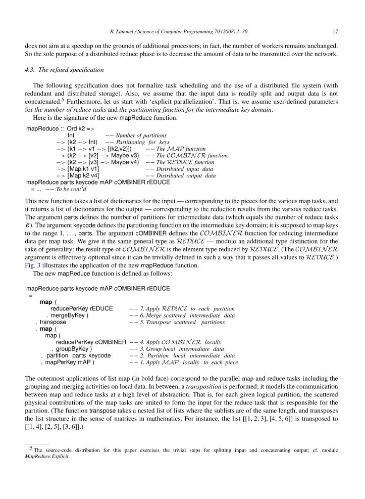
Here is the signature of the new mapReduce function:

mapReduce :: Ord k2 =>Int −− Number of partitions

−> (k2 −> Int) −− Partitioning for keys−> (k1 −> v1 −> [(k2,v2)]) −− TheMAP function−> (k2 −> [v2] −> Maybe v3) −− The COMBINER function−> (k2 −> [v3] −> Maybe v4) −− TheREDUCE function−> [Map k1 v1] −− Distributed input data−> [Map k2 v4] −− Distributed output data

mapReduce parts keycode mAP cOMBINER rEDUCE= ... −− To be cont’d

This new function takes a list of dictionaries for the input — corresponding to the pieces for the various map tasks, andit returns a list of dictionaries for the output — corresponding to the reduction results from the various reduce tasks.The argument parts defines the number of partitions for intermediate data (which equals the number of reduce tasksR). The argument keycode defines the partitioning function on the intermediate key domain; it is supposed to map keysto the range 1, . . . , parts. The argument cOMBINER defines the COMBINER function for reducing intermediatedata per map task. We give it the same general type as REDUCE — modulo an additional type distinction for thesake of generality: the result type of COMBINER is the element type reduced by REDUCE . (The COMBINERargument is effectively optional since it can be trivially defined in such a way that it passes all values to REDUCE .)Fig. 3 illustrates the application of the new mapReduce function.

The new mapReduce function is defined as follows:

mapReduce parts keycode mAP cOMBINER rEDUCE=

map (reducePerKey rEDUCE −− 7. Apply REDUCE to each partition

. mergeByKey ) −− 6. Merge scattered intermediate data. transpose −− 5. Transpose scattered partitions. map (

map (reducePerKey cOMBINER −− 4. Apply COMBINER locally

. groupByKey ) −− 3. Group local intermediate data. partition parts keycode −− 2. Partition local intermediate data. mapPerKey mAP ) −− 1. Apply MAP locally to each piece

The outermost applications of list map (in bold face) correspond to the parallel map and reduce tasks including thegrouping and merging activities on local data. In between, a transposition is performed; it models the communicationbetween map and reduce tasks at a high level of abstraction. That is, for each given logical partition, the scatteredphysical contributions of the map tasks are united to form the input for the reduce task that is responsible for thepartition. (The function transpose takes a nested list of lists where the sublists are of the same length, and transposesthe list structure in the sense of matrices in mathematics. For instance, the list [[1, 2, 3], [4, 5, 6]] is transposed to[[1, 4], [2, 5], [3, 6]].)

5 The source-code distribution for this paper exercises the trivial steps for splitting input and concatenating output; cf. moduleMapReduce.Explicit.


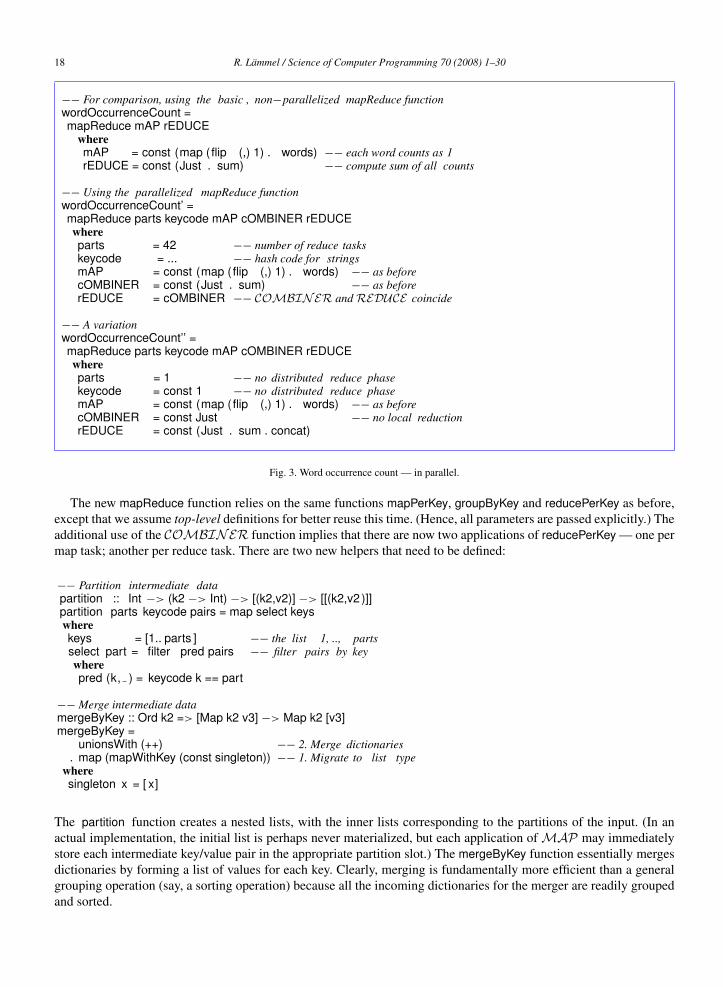
−− For comparison, using the basic , non−parallelized mapReduce functionwordOccurrenceCount =mapReduce mAP rEDUCE

wheremAP = const (map (flip (,) 1) . words) −− each word counts as 1rEDUCE = const (Just . sum) −− compute sum of all counts

−− Using the parallelized mapReduce functionwordOccurrenceCount’ =mapReduce parts keycode mAP cOMBINER rEDUCEwhereparts = 42 −− number of reduce taskskeycode = ... −− hash code for stringsmAP = const (map (flip (,) 1) . words) −− as beforecOMBINER = const (Just . sum) −− as beforerEDUCE = cOMBINER −− COMBINER andREDUCE coincide

−− A variationwordOccurrenceCount’’ =mapReduce parts keycode mAP cOMBINER rEDUCEwhereparts = 1 −− no distributed reduce phasekeycode = const 1 −− no distributed reduce phasemAP = const (map (flip (,) 1) . words) −− as beforecOMBINER = const Just −− no local reductionrEDUCE = const (Just . sum . concat)

Fig. 3. Word occurrence count — in parallel.

The new mapReduce function relies on the same functions mapPerKey, groupByKey and reducePerKey as before,except that we assume top-level definitions for better reuse this time. (Hence, all parameters are passed explicitly.) Theadditional use of the COMBINER function implies that there are now two applications of reducePerKey — one permap task; another per reduce task. There are two new helpers that need to be defined:

−− Partition intermediate datapartition :: Int −> (k2 −> Int) −> [(k2,v2)] −> [[(k2,v2 )]]partition parts keycode pairs = map select keyswherekeys = [1.. parts ] −− the list 1, .., partsselect part = filter pred pairs −− filter pairs by keywherepred (k, ) = keycode k == part

−− Merge intermediate datamergeByKey :: Ord k2 => [Map k2 v3] −> Map k2 [v3]mergeByKey =

unionsWith (++) −− 2. Merge dictionaries. map (mapWithKey (const singleton)) −− 1. Migrate to list type

wheresingleton x = [ x]

The partition function creates a nested lists, with the inner lists corresponding to the partitions of the input. (In anactual implementation, the initial list is perhaps never materialized, but each application of MAP may immediatelystore each intermediate key/value pair in the appropriate partition slot.) The mergeByKey function essentially mergesdictionaries by forming a list of values for each key. Clearly, merging is fundamentally more efficient than a generalgrouping operation (say, a sorting operation) because all the incoming dictionaries for the merger are readily groupedand sorted.


4.4. Implicit parallelization for reduction

If we assume that the input data is readily stored in a distributed file system, then we may derive the number ofmap tasks from the existing segmentation, thereby making the parallelism of the map phase ‘implicit’. Let us alsotry to make implicit other control parameters for parallel/distributed execution. Optimal values for the number ofreduce tasks and the partitioning function for the intermediate key domain may require problem-specific insights. Inthe following, we sketch a generic (and potentially suboptimal) method, which is based on a ‘quick scan’ over theresult of the map phase and a generic hash-code function for the key domain.

mapReduce mAP cOMBINER rEDUCE hash x =map (

reducePerKey rEDUCE −− 7. Apply REDUCE to each partition. mergeByKey ) −− 6. Merge intermediates per key

$ transpose −− 5. Transpose scattered partitions$ map (

map (reducePerKey cOMBINER −− 4. Apply COMBINER locally

. groupByKey ) −− 3. Group local intermediate data. partition parts keycode ) −− 2. Partition local intermediate data

$ y −− 1. Apply MAP locally to each piecewherey = map (mapPerKey mAP) x(parts,keycode) = quickScan hash y

This approach implies some synchronization costs; it assumes that all map tasks have been completed before thenumber of partitions is calculated, and the intermediate key/value pairs are associated with partitions, before, in turn,the reduce phase can be started. Here is a concrete proposal for quickScan:

quickScan :: (Data k2, Data v2) => (k2 −> Int) −> [[(k2,v2)]] −> ( Int , k2 −> Int)quickScan hash x = (parts, keycode)whereparts =

min maxParts −− Enforce bound$ flip div maxSize −− Compute number of partitions$ sum −− Combine sizes$ map (sum . map gsize) x −− Total data parallelism for size

keycode key =((hash key) ‘mod‘ parts) + 1

We leverage a generic size function, gsize, that is provided by Haskell’s generic programming library Data.Generics(admittedly based on Haskell’98 extensions). This size function implies the Data constraints for the intermediatekey and value domains in the type of quickScan. Further, this definition presumes two fixed limits maxSize, for themaximum size of each partition, and maxParts, for a cut-off limit for the number of partitions. For simplicity, themaximum size is not used as a strict bound for the size of partitions; it is rather used to determine the number ofpartitions under the idealizing assumption of uniform distribution over the intermediate key domain. As an aside, thedefinition of quickScan is given in a format that clarifies the exploitable parallelism. That is, sizes can be computedlocally per map task, and summed up globally. It is interesting to notice that this scheme is reminiscent of thedistributed reduce phase (without though any sort of key-based indexing).

4.5. Correctness of distribution

We speak of correct distribution if the result of distributed execution is independent of any variables in thedistribution strategy, such as numbers of map and reduce tasks, and the semi-parallel schedule for task execution.Without the extra COMBINER argument, a relatively obvious, sufficient condition for a correct distribution is this:(i) theREDUCE function is a proper reduction, and (ii) the order of intermediate values per key, as seen byREDUCE ,is stable w.r.t. the order of the input, i.e., the order of intermediate values for the distributed execution is the same asfor the non-distributed execution.


Instead of (ii) we may require (iii): commutativity for the reduction performed by REDUCE . We recall that thetype of REDUCE , as defined by the seminal MapReduce paper, goes beyond reduction in a narrow sense. As far aswe can tell, there is no intuitive, sufficient condition for correct distribution once we give up on (i).

Now consider the case of an additional COMBINER argument. If COMBINER and REDUCE implementthe same proper reduction, then the earlier correctness condition continues to apply. However, there is no point inhaving two arguments, if they were always identical. If they are different, then, again, as far as we can tell, there is nointuitive, sufficient condition for correct distribution.

As an experiment, we formalize the condition for correctness of distribution for arbitrary COMBINER andREDUCE functions, while essentially generalizing (i) + (iii). We state that the distributed reduction of any possiblesegmentation of any possible permutation of a list l of intermediate values must agree with the non-distributedreduction of the list.

For all k of type k2,

for all l of type [v2],for all l ′ of type [[v2]] such that concat l ′ is a permutation of l

REDUCE k (unJusts (COMBINER k l))= REDUCE k (concat (map (unJusts . COMBINER k) l ′))

where

unJusts (Just x ) = [ x]unJusts Nothing = []

We contend that the formal property is (too) complicated.

5. Sawzall’s aggregators

When we reflect again on the reverse-engineered programming model in the broader context of (parallel) data-processing, one obvious question pops up. Why would we want to restrict ourselves to keyed input and intermediatedata? For instance, consider the computation of any sort of ‘size’ of a large data set (just as in the case of the quickscan that was discussed above). We would want to benefit from MapReduce’s parallelism, even for scenarios that donot involve any keys. One could argue that a degenerated key domain may be used when no keys are needed, butthere may be a better way of abstracting from the possibility of keys. Also, MapReduce’s parallelism for reductionrelies on the intermediate key domain. Hence, one may wonder how parallelism is to be achieved in the absence of a(non-trivial) key domain.

Further reflection on the reverse-engineered programming model suggests that the model is complicated, once twoarguments, REDUCE and COMBINER, are to be understood. The model is simple enough, if both argumentsimplement exactly the same function. If the two arguments differ, then the correctness criterion for distribution is notobvious enough. This unclarity only increases once we distinguish types for intermediate and output data (and perhapsalso for data used for the shake-hand betweenREDUCE and COMBINER). Hence, one may wonder whether thereis a simpler (but still general) programming model.

Google’s domain-specific language Sawzall [26], with its key abstraction, aggregators, goes beyond MapReduce inrelated ways. Aggregators are described informally in the Sawzall paper — mainly from the perspective of a languageuser. In this section, we present the presumed, fundamental characteristics of aggregators.

We should not give the impression that Sawzall’s DSL power can be completely reduced to aggregators. In fact,Sawzall provides a rich library, powerful ways of dealing with slightly abnormal data, and other capabilities, whichwe skip here due to our focus on the schemes and key abstractions for parallel data-processing.

5.1. Sawzall’s map and reduce

Sawzall’s programming model relies on concepts that are very similar to those of MapReduce. A Sawzall programprocesses a record as input and emits values for aggregation. For instance, the problem of aggregating the size of a setof CVS submission records would be described as follows — using Sawzall-like notation:


proto “CVS.proto” −− Include types for CVS submission recordscvsSize : table sum of int; −− Declare an aggregator to sum up intsrecord : CVS submission = input; −− Parse input as a CVS submissionemit cvsSize← record.size; −− Aggregate the size of the submission

The important thing to note about this programming style is that one processes one record at the time. That is, thesemantics of a Sawzall program comprises the execution of a fresh copy of the program for each record; the per-record results are emitted to a shared aggregator. The identification of the kind of aggregator is very much like theidentification of a REDUCE function in the case of a MapReduce computation.

The relation between Sawzall and MapReduce has been described (in the Sawzall paper) as follows [26]: “TheSawzall interpreter runs in the map phase. [...] The Sawzall program executes once for each record of the data set.The output of this map phase is a set of data items to be accumulated in the aggregators. The aggregators run inthe reduce phase to condense the results to the final output”. Interestingly, there is no mentioning of keys in thisexplanation, which suggests that the explanation is incomplete.

5.2. List homomorphisms

The Sawzall paper does not say so, but we contend that the essence of a Sawzall program is to identify thecharacteristic arguments of a list homomorphism [4,9,28,17,8]: a function to be mapped over the list elements as wellas the monoid to be used for the reduction. (A monoid is a simple algebraic structure: a set, an associative operation,and its unit.) List homomorphisms provide a folklore tool for parallel data processing; they are amenable to massiveparallelism in a tree-like structure; element-wise mapping is performed at the leafs, and reduction is performed at allother nodes.

In the CVS example, given above, the conversion of the generically typed input to record (which is of the CVSsubmission type), composed with the computation of the record’s size is essentially the mapping part of a listhomomorphism and the declaration of the ‘sum’ aggregator, to which we emit, identifies the monoid for the reductionpart of the list homomorphism. For comparison, let us translate the Sawzall-like code to Haskell. We aggregate thesizes of CVS submission records in the monoid Sum — a monoid under addition:

import CVS −− Include types for CVS submission recordsimport Data.Monoid −− Haskell’s library for reductionimport Data.Generics −− A module with a generic size function

cvsSize input = Sum (gsize x)wherex :: CvsSubmissionx = read input

Here, Sum injects an Int into the monoid under addition. It is now trivial to apply cvsSize to a list of CVS submissionrecords and to reduce the resulting list of sizes to a single value (by using the associative operation of the monoid).

As an aside, Google’s Sawzall implementation uses a proprietary, generic record format from which to recoverdomain-specific data by means of ‘parsing’ (as opposed to ‘strongly typed’ input). In the above Haskell code, weapproximate this overall style by assuming String as generic representation type and invoking the normal readoperation for parsing. In subsequent Haskell snippets, we take the liberty to neglect such type conversions, forsimplicity.

Haskell’s monoids: There is the following designated type class:

class Monoid awheremappend :: a −> a −> a −− An associative operationmempty :: a −− Identity of ’ mappend’mconcat :: [a] −> a −− Reductionmconcat = foldr mappend mempty −− Default definition


−− Process a flat listphasing, fusing :: Monoid m => (x −> m) −> [x] −> mphasing f = mconcat . map ffusing f = foldr ( mappend . f) mempty

−− Process lists on many machinesphasing ’, fusing ’ :: Monoid m => (x −> m) −> [[x]] −> mphasing’ f = mconcat . map (phasing f)fusing ’ f = mconcat . map (fusing f)

−− Process lists on many racks of machinesphasing ’’, fusing ’’ :: Monoid m => (x −> m) −> [[[x]]] −> mphasing ’’ f = mconcat . map (phasing’ f)fusing ’’ f = mconcat . map (fusing’ f )

Fig. 4. List-homomorphisms for 0, 1 and 2 levels of parallelism.

The essential methods are mappend and mempty, but the class also defines an overloaded methods for reduction:mconcat. We note that this method, by default, is right-associative (as opposed to left associativity as Lisp’s default).For instance, Sum, the monoid under addition, which we used in the above example, is defined as follows:

newtype Sum a = Sum { getSum :: a }

instance Num a => Monoid (Sum a)wheremempty = Sum 0Sum x ‘mappend‘ Sum y = Sum (x + y)

More Haskell trivia: A newtype (read as ‘new type’) is very much like a normal data type in Haskell (keyword data instead ofnewtype) — except that a new type defines exactly one constructor (cf. the Sum on the right-hand side) with exactly one component(cf. the component of the parametric type a). Thereby it is clear that a new type does not serve for anything but a type distinctionbecause it is structurally equivalent to the component type.

3

In the case of MapReduce, reduction was specified monolithically by means of theREDUCE function. In the case ofSawzall, reduction is specified by identifying its ingredients, in fact, by naming the monoid for reduction. Hence, theactual reduction can still be composed together in different ways. That is, we can form a list homomorphism in twoways [21,20]:

−− Separated phases for mapping and reductionphasing f = mconcat . map f −− first map, then reduce

−− Mapping and reduction ‘fused’fusing f = foldr ( mappend . f) mempty −− map and reduce combined

If we assume nested lists in the sense of data parallelism, then we may also form list homomorphisms that makeexplicit the tree-like structure of reduction. Fig. 4 illustrates this simple idea for 1 and 2 levels of parallelism. The firstlevel may correspond to multiple machines; the second level may correspond to racks of machines. By now, we coverthe topology for parallelism that is assumed in the Sawzall paper; cf. Fig. 5.

We can test the Haskell transcription of the Sawzall program for summing up the size of CVS submission records.Given inputs of the corresponding layout (cf., many records, many machines, many racks), we aggregate sizes fromthe inputs by applying the suitable list-homomorphism scheme to cvsSize:

many records :: [String ]many machines :: [[ String ]]many racks :: [[[ String ]]]


Fig. 5. The above figure and the following quote is taken verbatim from [26]: “Five racks of 50–55 working computers each, with fourdisks per machine. Such a configuration might have a hundred terabytes of data to be processed, distributed across some or allof the machines. Tremendous parallelism can be achieved by running a filtering phase independently on all 250+ machines andaggregating their emitted results over a network between them (the arcs). Solid arcs represent data flowing from the analysismachines to the aggregators; dashed arcs represent the aggregated data being merged, first into one file per aggregation machineand then to a single final, collated output file”.

test1 = fusing cvsSize many recordstest2 = fusing ’ cvsSize many machinestest3 = fusing ’’ cvsSize many racks

An obvious question is whether Sawzall computations can be fairly characterized to be generally based on listhomomorphisms, as far as (parallel) data-processing power is concerned. This seems to be the case, as we willsubstantiate in the sequel.

5.3. Tuple aggregators

Here is the very first code sample from the Sawzall paper (modulo cosmetic edits):

count : table sum of int; −− Aggregator: counts recordstotal : table sum of float; −− Aggregator: totals all recordssum of squares : table sum of float −− Aggregator: totals squares;

x : float = input; −− Convert input to floatemit count← 1; −− Count as 1emit total← x; −− Add input to totalemit sum of squares← x * x; −− Add square of input

Conceptually, this Sawzall program performs three aggregations over the input. Of course, for the sake of efficiency,we wish to perform only a single, actual pass over the input. We can exploit the monoid of tuples. The so-called‘banana split’ property of foldr implies that the results of multiple passes coincide with the projections of a singlepass [22,20]. Thus, the Sawzall program is translated to a Haskell program (which is, by the way, shorter and morepolymorphic) as follows:

firstSawzall x = (Sum 1, Sum x, Sum (x∗x))

The monoid of triplets is readily defined (in Haskell’s library) as follows:


−− Ascending sets with opaque representationnewtype Ord x => AscendingSet x =

AscendingSet { getAscendingSet :: [x] }

−− Construct a set from a listmkAscendingSet :: Ord x => [x] −> AscendingSet xmkAscendingSet = AscendingSet . quicksort compare

−− Sets as a monoidinstance Ord x => Monoid (AscendingSet x)wheremempty = AscendingSet []mappend x y = AscendingSet (merge compare (getAscendingSet x)

(getAscendingSet y))

−− A helper for merging two sorted listsmerge c [] y = ymerge c x [] = xmerge c xs ys = case c (head xs) (head ys) of

EQ −> (head xs) : merge c ( tail xs ) ( tail ys)LT −> (head xs) : merge c ( tail xs) ysGT −> (head ys) : merge c xs ( tail ys)

−− Quick sort for setsquicksort c [] = []quicksort c (x:xs) = quicksort c lt ++ [x] ++ quicksort c gtwhere lt = filter ((==) LT . flip c x) xs

gt = filter ((==) GT . flip c x) xs

Fig. 6. A monoid of ascending sets.

instance ( Monoid a, Monoid b, Monoid c) => Monoid (a,b,c)wheremempty = (mempty, mempty, mempty)mappend (a1,b1,c1) (a2,b2,c2) = (mappend a1 a2, mappend b1 b2, mappend c1 c2)

Thus, the binary operation for tuples is defined by applying binary operations in a component-wise manner, and theunit is just the tuple of units for the component types. In contrast, Sawzall uses an ‘imperative’ style: first emit tocount, then to total, etc. This style is actually somewhat misleading because it is hard to think of a useful exploitationof ‘statement order’ within the bounds of Sawzall’s programming model.

5.4. Collection aggregators

The monoid’s type may (of course) also correspond to a collection type. For instance, consider a monoid of setsordered in ascending order of the element type. The Haskell library readily covers sets and ordering, but Fig. 6 showsa simple implementation for illustrative purposes. The only ‘public’ way of populating the type is by means of theconstructor mkAscendingSet. The monoid’s mappend operation is essentially a union operation on (ordered) sets; itperforms a merge step (in the sense of merge sort) on the opaque list representation.

Let us assume that we want to derive a (sorted and unique) word list for a given repository of documents. InSawzall-like notation, this may be accomplished as follows (assuming an aggregator form ‘table ascending set’):


wordList : table ascending set of string;x : string = input;for each w in x.wordsemit wordList← w;

Here is a Haskell transcription:

wordList =mkAscendingSet −− Emit words for ascending order

. words −− Split record into words

An interesting difference between the two styles is that the Sawzall-like code issues multiple emissions (several words)per input record, whereas the Haskell code issues one emission (a set of words). We will return to this observation ina second.

5.5. Indexed aggregators

The Sawzall examples so far did not involve keyed data. We recall that the MapReduce model makes a point aboutkeyed data. One can easily model the typical MapReduce example in Sawzall by means of indexed aggregators. Let usrevisit the problem of counting occurrences of words, which we used earlier to illustrate MapReduce. Words serve asindex values for the purpose of a Sawzall encoding — just as much as the representation type for words (i.e., strings)served as ‘key domain’ for MapReduce. Thus, in Sawzall-like notation (using square brackets for indexing):

wordOccurrenceCount : table sum[word: string] of int;x : string = input;for each w in x.wordsemit wordOccurrenceCount[w]← 1;

Here is a Haskell transcription:

wordOccurrenceCount =mkIndexedBy −− Combines counts

. map (flip (,) ( Sum (1::Int ))) −− Count each word as 1


Hence, each record is mapped to a list of string/int pairs, which is then turned into a sort of dictionary; cf.mkIndexedBy. The type Map of the Data.Map module is almost appropriate. In fact, the type readily implementsthe Monoid interface, but in a way that is inappropriate for our purposes.

instance Ord k => Monoid (Map k v)wheremempty = emptymappend = union −− left−biased unionmconcat = unions −− left−associative fold

This instance does not assume the value type of the dictionary to be a monoidal type. We want the associative operationof the ‘inner’ monoid to be applied when dictionaries are combined. Hence, we define a new type, IndexedBy, thatserves for nothing but a type distinction that allows us to vary the monoid instance for indexed aggregators:

newtype (Ord k, Monoid v) => IndexedBy k v= IndexedBy { getMap :: Map k v }

Here is the constructor that we used in the sample code:

mkIndexedBy :: (Ord k, Monoid v) => [(k,v)] −> IndexedBy k vmkIndexedBy = IndexedBy . fromList


The Monoid instance uses unionWith mappend instead of union:

instance ( Ord k, Monoid v) => Monoid (IndexedBy k v)wheremempty = IndexedBy memptymappend (IndexedBy f) (IndexedBy g) = IndexedBy (unionWith mappend f g)

5.6. Generalized monoids

The two previous examples (for word lists and word-occurrence counting) exemplified differences between Sawzalland Haskell style — regarding the granularity and the typing of ‘emissions’:

• The strict, monoidal Haskell style only admits one emission per input record, whereas the free-wheeling Sawzallstyle admits any number of emissions.• The strict, monoidal Haskell style requires emissions to be of the monoid’s type, whereas the free-wheeling Sawzall

style covers a special case for collection-like aggregators. That is, an emission can be of the element type.

These differences do not affect expressiveness in a formal sense, as we have clarified by the transcription of theexamples. However, the differences may negatively affect the convenience of the Haskell style, and also challenge anefficient implementation of certain aggregators.

A simple extension of the Monoid interface comes to rescue. Essentially, we need to model ‘emissions toaggregators’. We define a new type class Aggregator as a subclass of Monoid for this purpose. The Aggregator typeclass comes with two designated type parameters, one for the underlying monoid, another for the emission type; thereis a method mInsert for insertion (say, emission):

class Monoid m => Aggregator e m | e −> mwheremInsert :: e −> m −> m−− m, the monoid’s type−− e, for the type of ‘ elements ’ to be inserted .

There is also a so-called functional dependency e −> m, which states that an emission type determines theaggregator type. This implies programming convenience because the aggregator type can be therefore ‘inferred’.(Multi-parameter type classes with functional dependencies go beyond Haskell 98, but they are well-understood [31],well-implemented and widely used.)

In the case of non-collection-like aggregators, e equals m, and mInsert equals mappend. In the case of collection-like aggregators, we designate a new type to emissions, and map mInsert to a suitable ‘insert’ operation of thecollection type at hand. Fig. 7 instantiates the Aggregator type class for a few monoids. The schemes for listhomomorphisms (say, one machine vs. many machines vs. multiple racks) are easily generalized. Separation ofmapping and reduction is not meaningful for this generalization; only the more efficient, fused form is admittedby the type of mInsert. Thus:

−− Process a flat listinserting :: Aggregator e m => (x −> e) −> [x] −> minserting f = foldr ( mInsert . f ) mempty

−− Process lists on many machinesinserting ’ :: Aggregator e m => (x −> e) −> [[x]] −> minserting ’ f = mconcat . map (inserting f )

−− Process lists on many racks of machinesinserting ’’ :: Aggregator e m => (x −> e) −> [[[x]]] −> minserting ’’ f = mconcat . map (inserting’ f )


−− Trivial instance for monoid under additioninstance Num x => Aggregator (Sum x) (Sum x)wheremInsert = mappend

−− Emission type for AscendingSetnewtype Ord x => AscendingSetElement x =

AscendingSetElement { getAscendingSetElement :: x }

−− Generalized monoid: AscendingSetinstance Ord x => Aggregator (AscendingSetElement x) (AscendingSet x)wheremInsert x = AscendingSet

. insert compare (getAscendingSetElement x)

. getAscendingSet

−− Helper for inserting an element into a sorted setinsert c x [] = [x]insert c x ys = case c x (head ys) of

EQ −> x : ( tail ys)LT −> x : ysGT −> (head ys) : insert c x ( tail ys)

−− Emission type for IndexedBydata (Ord k, Monoid v) => KeyValuePair k v = KeyValuePair k v

−− Generalized monoid: IndexedByinstance ( Ord k, Monoid v) => Aggregator (KeyValuePair k v) (IndexedBy k v)wheremInsert (KeyValuePair k v) (IndexedBy f) =

IndexedBy $ insertWith mappend k v f

Fig. 7. Illustrative Aggregator instances.

The emission type is more flexible now, but we still need to admit multiple emissions per input record (other than byexplicitly invoking reduction). Strong static typing (of Haskell) implies that we must differentiate single vs. multipleemissions somehow explicitly. In fact, the Aggregator type class allows us to admit lists of emissions as an additionalemission type for any aggregator. To this end, we designate an emission type constructor, Group, as follows:

newtype Group e =Group { getGroup :: [e ] }

instance Aggregator e m => Aggregator (Group e) mwheremInsert es = mInsertList $ getGroup eswheremInsertList = flip $ foldr mInsert

Hence, multiple emissions are grouped as a single emission, and during insert, they are ‘executed’ one-by-one; cf.the definition of the function mInsertList. With this machinery in place, we can revise the examples for word lists andword-occurrence counting such that multiple words or key/value pairs are emitted, without any local reduction.

wordList =Group −− Group emissions per record

. map AscendingSetElement −− Emit words for ascending order



wordOccurrenceCount =Group −− Group emissions per record

. map (flip KeyValuePair (Sum (1::Int ))) −− Count each word as 1


Essentially, the expression of grouping in the Haskell code is the declarative counterpart for the imperative for-eachloop in MapReduce or Sawzall style.

5.7. Multi-set aggregators

Let us attempt another simplification for the special case of indexed aggregation with counting. We contend thatthe assembly of key/value pairs, as shown so far, is tedious; we needed to couple up elements with the trivial count 1.Instead we may model this problem by means of an aggregator for multi-sets. Thus:

wordOccurrenceCount =Group −− Group emissions per record

. map MultiSetElement −− Add each word to a multi−set


We can trivially implement multi-set aggregators in terms of indexed aggregators on a monoid for addition. In fact,we do not even need a new aggregator type. Instead, we only introduce a new emission type MultiSetElement for theexisting monoid IndexedBy.

−− Emission type for multi−setsnewtype Ord k => MultiSetElement k =

MultiSetElement { getMultiSetElement :: k }

−− Multi−set aggregation in terms of indexed aggregationinstance Ord k => Aggregator (MultiSetElement k) (IndexedBy k (Sum Int))wheremInsert k = mInsert (KeyValuePair (getMultiSetElement k) (Sum 1))

5.8. Correctness of distribution

Compared to MapReduce (cf. Section 4.5), the situation is much simpler and well-understood because of theexisting foundations for list homomorphisms. The computation result is independent of the actual data distributionover machines and racks. That is, associativity of the monoid’s binary operation suffices to imply correctness forthe staged reduction at the machine level, followed by the rack level, followed by the global level — as long assub-reductions are composed in the order of the input, or a commutative monoid must be used.

It remains to clarify generalized monoids in algebraic terms. The insert operation must be such that it could also beused to turn an emission into a value of the monoid’s type so that the basic monoidal scheme of list homomorphismsis sufficient. Thus:

mInsert e m = mInsert e mempty ‘mappend‘ m

5.9. Sawzall vs. MapReduce

Let us try to understand the precise relationship between MapReduce and Sawzall. In doing so, we use thearchetypal problem of counting occurrences of words for inspiration, as before.

The MapReduce implementation of [10] distributes the reduce phase by means of partitioning the intermediate keydomain; recall Fig. 2. We face an ‘any-to-any’ connectivity network between MapReduce’s map and reduce tasks.That is, each single map task may compute intermediate data for all the different reduce tasks.


In contrast, the Sawzall implementation of [26] distributes reduction (aggregation) in a hierarchical (network-topology-based manner): reduction per machine, followed by reduction per rack, followed by final, global reduction;cf. Fig. 5. Communication is hence organized in tree-like shape, as opposed to ‘any-to-any’.

Hence the implementation of Sawzall, as described in [26], cannot possibly be based on the implementation ofMapReduce, as described in [10], despite the fact that the Sawzall paper seems to say so. Presumably, Google usesseveral, fundamentally different implementations of MapReduce (and Sawzall). The distribution model published forSawzall is both simpler and more general than the one published for MapReduce. Monoidal reduction (fused withmapping) organized in tree-like shape does not take any dependency on the potentially keyed status of the monoid’stype. The published model for MapReduce is biased towards the monoid for indexed aggregation.

A remaining question may be whether the kind of data-structural knowledge of a MapReduce implementation canbe re-casted to a Sawzall implementation. In particular, consider the treatment of grouping by MapReduce, where mapworkers perform grouping locally and reduce workers perform merging. We contend that implementations of monoidsmay model such distribution details (without breaking the abstraction of monoids though). In fact, the generalizedmonoid IndexedBy, as it was shown earlier, in combination with the scheme for parallel list homomorphisms, isexactly set up to perform a kind of a parallel-merge-all strategy [11]. As a consequence, we also do not see the needfor the complicated distinction ofREDUCE and COMBINER— as assumed by the MapReduce implementations.

6. Conclusion

MapReduce and Sawzall must be regarded as an impressive testament to the power of functional programming —to list processing in particular. Google has fully unleashed the power of list homomorphisms and friends for massive,simple and robust parallel programming. The original formulations of the models for MapReduce and Sawzall slightlyconfuse and hide some of the underlying concepts, which is where the present paper aims to contribute. Our analysisof Google’s publications may help with a deeper understanding of the ramifications of Google’s results.

We have systematically used the typed functional programming language Haskell for the discovery of a rigorousdescription of the MapReduce programming model and its advancement as the domain-specific language Sawzall. Asa side effect, we deliver a relatively general illustration for the utility of functional programming in a semi-formalapproach to design with excellent support for executable specification. This illustration may motivate others to deployfunctional programming for their future projects, be in the context of distributed computing, data processing, orelsewhere.

The following capabilities of functional programming are instrumental in the process of software design: strongtype checking, full type inference, powerful abstraction forms, compositionality, and algebraic reasoning style. Thisinsight has been described more appropriately by Hughes, Thompson, and surely others [19,33].

Acknowledgments

I would like to acknowledge feedback I received through presentations on the subject at: University of Innsbruck(January 2006), University of Nottingham (January 2006), Rice University in Texas (July 2006), University ofNebraska at Omaha (April 2007), and Physikzentrum Bad Honnef (May 2007).

References

[1] L. Augusteijn, Sorting morphisms, in: S. Swierstra, P. Henriques, J. Oliveira (Eds.), 3rd International Summer School on Advanced FunctionalProgramming, in: LNCS, vol. 1608, Springer-Verlag, September 1998, pp. 1–27.

[2] J.W. Backus, Can programming be liberated from the von Neumann style? A functional style and its algebra of programs, Communicationsof the ACM 21 (8) (1978) 613–641.

[3] R. Bird, O. de Moor, Algebra of Programming, Prentice-Hall, Inc., 1996.[4] R.S. Bird, An introduction to the theory of lists, in: Proceedings of the NATO Advanced Study Institute on Logic of Programming and Calculi

of Discrete Design, Springer-Verlag, 1987, pp. 5–42.[5] G.E. Blelloch, Programming parallel algorithms, Communications of the ACM 39 (3) (1996) 85–97.[6] A. Borodin, J.E. Hopcroft, Routing, merging and sorting on parallel models of computation, in: STOC’82: Proceedings of the Fourteenth

Annual ACM Symposium on Theory of Computing, ACM Press, 1982, pp. 338–344.[7] L. Bouge, P. Fraigniaud, A. Mignotte, Y. Robert (Eds.), Proceedings of the 2nd International Euro-Par Conference on Parallel Processing, 2

volumes, EURO-PAR’96, in: LNCS, vol. 1123–1124, Springer-Verlag, 1996.[8] W.-N. Chin, J. Darlington, Y. Guo, Parallelizing conditional recurrences, in: Bouge et al. [7], Volume 1/2, pp. 579–586.


[9] M. Cole, Parallel Programming with List Homomorphisms, Parallel Processing Letters 5 (1995) 191–203.[10] J. Dean, S. Ghemawat, MapReduce: Simplified Data Processing on Large Clusters, in: OSDI’04, 6th Symposium on Operating Systems

Design and Implementation, Sponsored by USENIX, in cooperation with ACM SIGOPS, 2004, pp. 137–150.[11] D.J. DeWitt, S. Ghandeharizadeh, D.A. Schneider, A. Bricker, H.-I. Hsiao, R. Rasmussen, The Gamma Database Machine Project, IEEE

Transactions on Knowledge and Data Engineering 2 (1) (1990) 44–62.[12] E. Gamma, R. Helm, R. Johnson, J. Vlissides, Design Patterns, Addison Wesley, 1995.[13] S. Ghemawat, H. Gobioff, S.-T. Leung, The Google file system, in: 19th ACM Symposium on Operating Systems Principles, Proceedings,

ACM Press, 2003, pp. 29–43.[14] J. Gibbons, A pointless derivation of radix sort, Journal of Functional Programming 9 (3) (1999) 339–346.[15] J. Gibbons, Calculating Functional Programs, in: R.C. Backhouse, R.L. Crole, J. Gibbons (Eds.), Algebraic and Coalgebraic Methods in

the Mathematics of Program Construction, International Summer School and Workshop, 10–14 April, Oxford, UK, 2000, Revised Lectures,in: LNCS, vol. 2297, Springer-Verlag, 2002, pp. 149–202.

[16] J. Gibbons, G. Jones, The under-appreciated unfold, in: ICFP ’98: Proceedings of the third ACM SIGPLAN International Conference onFunctional Programming, ACM Press, 1998, pp. 273–279.

[17] S. Gorlatch, Systematic efficient parallelization of scan and other list homomorphisms, in: Bouge et al. [7], Volume 2/2, pp. 401–408.[18] D. Hirschberg, Fast parallel sorting algorithms, Communications of the ACM 21 (8) (1978) 657–661.[19] J. Hughes, Why functional programming matters, The Computer Journal 32 (2) (1989) 98–107.[20] G. Hutton, A tutorial on the universality and expressiveness of fold, Journal of Functional Programming 9 (4) (1999) 355–372.[21] G. Malcolm, Algebraic data types and program transformation, Ph.D. Thesis, Groningen University, 1990.[22] E. Meijer, Calculating compilers, Ph.D. Thesis, Nijmegen University, 1992.[23] E. Meijer, M. Fokkinga, R. Paterson, Functional programming with bananas, lenses, envelopes and barbed wire, in: J. Hughes (Ed.),

Proceedings of 5th ACM Conference on Functional Programming Languages and Computer Architecture, FPCA’91, in: LNCS, vol. 523,Springer-Verlag, 1991, pp. 124–144.

[24] S. Peyton Jones (Ed.), Haskell 98 Language and Libraries — The Revised Report, Cambridge University Press, Cambridge, England, 2003.[25] S. Peyton Jones, M. Shields, Lexically scoped type variables, March 2004. Available at

http://research.microsoft.com/Users/simonpj/papers/scoped-tyvars/.[26] R. Pike, S. Dorward, R. Griesemer, S. Quinlan, Interpreting the data: Parallel analysis with Sawzall, in: Dynamic Grids and Worldwide

Computing, Scientific Programming 14 (2006) (special issue).[27] D.B. Skillicorn, Architecture-independent parallel computation, IEEE Computer 23 (12) (1990) 38–50.[28] D.B. Skillicorn, Foundations of Parallel Programming, in: Cambridge Series in Parallel Computation, No. 6, Cambridge University Press,

1994.[29] D.B. Skillicorn, D. Talia, Models and languages for parallel computation, ACM Computing Surveys 30 (2) (1998) 123–169.[30] G.L. Steele Jr., Common Lisp: The Language, 2nd edition, Digital Press, 1990.[31] P.J. Stuckey, M. Sulzmann, A theory of overloading, ACM TOPLAS 27 (6) (2005) 1216–1269.[32] D. Taniar, J.W. Rahayu, Parallel database sorting, Information Sciences and Applications: An International Journal 146 (1–4) (2002) 171–219.[33] S. Thompson, The Craft of Functional Programming, Addison Wesley, 1996. 2nd edition in 1999.

http://research.microsoft.com/Users/simonpj/papers/scoped-tyvars/

Google’s MapReduce programming model — …€™s MapReduce programming model — Revisited Ralf...

Documents

Transcript of Google’s MapReduce programming model — …€™s MapReduce programming model — Revisited Ralf...