Goddard-DR-2010

The Challenges of Ground-based Astronomical Array Imaging at Far-Infrared Wavelengths

Attila KovácsUniversity of Minnesota

Part II

Scanning Strategies

Part I

Data Reduction

A Galaxy far far away...(10 Gly, 35K)

atmosphere(300K)

Bolometers

1/f noise

Unstable gain/noise

Microphonics

EM pickup

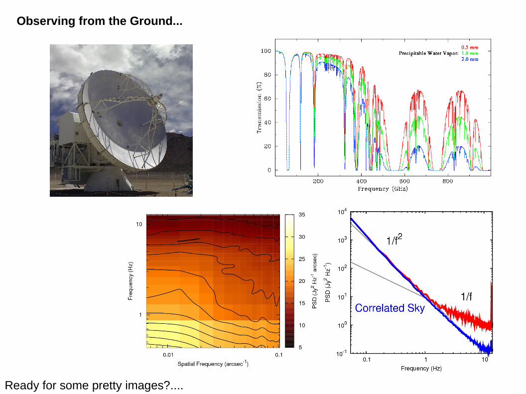
Observing from the Ground...

Ready for some pretty images?....

The Galactic Center of the Milky Way

LABOCA (870um)

Visible light

SABOCA (350um) Optical and Near Infrared

LABOCA (870um) 870um polarized flux

GISMO (2 mm)

The Orion Molecular Cloud(OMC-1)

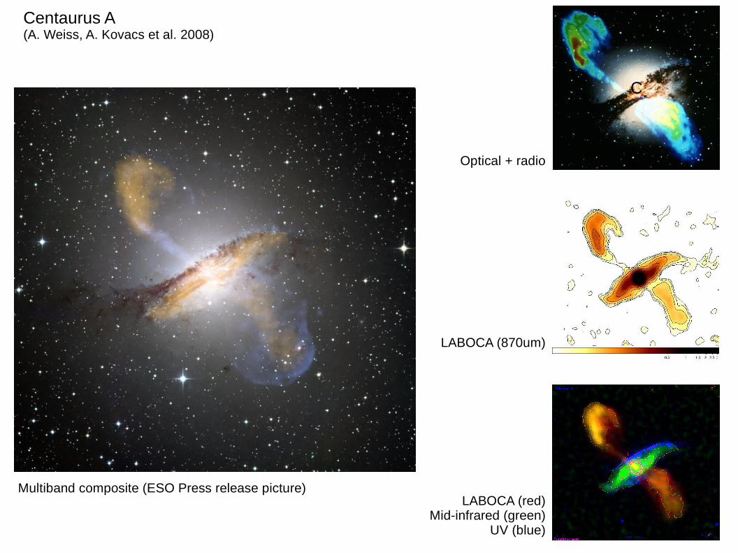
C

Multiband composite (ESO Press release picture)

Centaurus A(A. Weiss, A. Kovacs et al. 2008)

Optical + radio

LABOCA (870um)

LABOCA (red)Mid-infrared (green)

UV (blue)

50 arcsec

Optimally (Wiener) filtered Around diffraction limit Slightly deconvolved

SHARC-2 350 um

Kovacs et al., in prep

Distant Galaxies

30 arcmin 3 arcmin

LABOCA CDFS deep field survey(A. Weiss & A. Kovacs)

Hubble Ultra Deep Field(optical)

LABOCA CDFS deep field survey(A. Weiss & A. Kovacs)

Hubble Ultra Deep Field(optical)

30 arcmin

Part I

Data Reduction

Typical Object Brightness...

ChoppingDifferential Signals

Fast switching of detectors between source and blank sky.Analyze difference signals.

E.g. 45” switching at 4 Hz for SHARC

Problems

Differencing Noise(2x observing time)

Insensitivity to CertainSpatial Components

Duty Cycle

Striping(Imperfect Sky Removal)

Observing Strategies for Imaging Arrays SPIE 2008 -- Marseille

Large Arrays

SHARC-2

LABOCA

The Array Imaging Challenge

High background

Unstable detectors

Faint signals

Large data volumes(100—10,000 pixels 10--100 Hz readout)

Do at least as well as chopping techniques...

Introducing CRUSH...

Comprehensive Reduction Utility for SHARC-2(PhD thesis, Caltech 2006)

Also used for LABOCA, SABOCA, ASZCA, ArTeMiS, PolKa, GISMO...

Offsprings: sharcsolve (C. D. Dowell), BoA (F. Schuller, A. Beelen et al.)

40K lines of Java code (and growing...)

Fast (~1GB/min on 4-core HT CPUs)...

Low overheads.

Future: more instrument, interferometry, other high background applications...

http://www.submm.caltech.edu/~sharc/crush

(2003 -- now)

Direct Mapping(lossless)

Pallas in 1 min(350um)

spectratime-streams

Pixel-to-pixelcovariance

SHARC-2

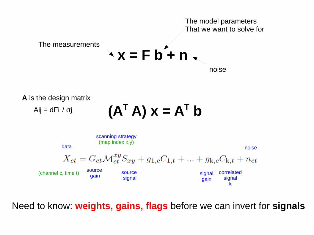
x = F b + n

(AT A) x = AT b

The model parametersThat we want to solve for

noise

The measurements

A is the design matrix

Aij = dFi

/ σj

Need to know: weights, gains, flags before we can invert for signals

(channel c, time t)

scanning strategy(map index x,y)

data

source gain

source signal

signalgain

correlatedsignal

k

noise

one term at a time...

Incremental solutions

Correlated signalincrementgain

Maximum-likelihood estimator

Can use other statistical estimators too...

residual

After Correlated Signal Removal


spectratime-streams


SHARC-2

Maximum likelihood gain increment

Can solve for gains too....

After sky gains...


spectratime-streams


SHARC-2

Calculating noise weights...

assuming

Channel weights:

Time weights:

The devil is in the detail:

Specifically in calculating Pt and Pc right.

Else unstable solutions...

After 6 iterations...


spectratime-streams


SHARC-2

LABOCA (850um)

Direct mapping After sky removal Decorrelating cables

Astronomical signal(Uranus @ 850um)

Relative pixel gains pixel noise

LABOCA (850um)

LABOCA (870um) SHARC-2 (350um)

Typical further steps:

- Decorrelate instrumental signals.

- Remove sky gradients

- Channel flagging by gain

- Flag noisy pixels

- Despiking

- Noise whitening

Direct Maximum-Likelihood Clipped model (>1 Jy) Iterated with clipped model

The Orion Molecular Cloud(OMC-1)

SABOCA (350um) Optical and Near Infrared

GISMO 2-mm Camera

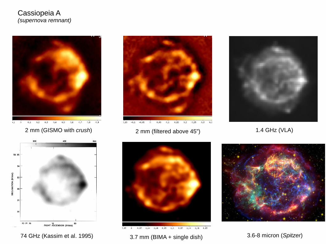
74 GHz (Kassim et al. 1995) 3.7 mm (BIMA + single dish)

1.4 GHz (VLA)2 mm (filtered above 45”)2 mm (GISMO with crush)

3.6-8 micron (Spitzer)

Cassiopeia A(supernova remnant)

The Galactic Center at 850um with LABOCA

Data Reduction Summary

Works well (better than SVD of PCA)...

Fast (~1 GB/min on a modern PC)

Distributable (for cluster computing)

Linear computing requirement

Low overheads

Lets the astronomer decide what's best....

Part II

Scanning Strategies

Observing Mode Wish List

Noise Resistance (esp. 1/f)

Large-Scale Sensitivity

Coverage

Dynamic Range

Feasibility of Implementation

Sensitivity to Large Scales

Scanning Wide

m0 = 1.000

m2 = 1.000

m1 = 1.000

Random

Noise ResistanceSpectral Noise Locations

Stationary noise (in time and in space) is characterized by its powerspectrum of independent components.

Projections of a spectral cube

Correlated Noise(atmosphere, T-fluctiation)



1/f Noise



1/f Noise

Sky Noise


Narrow-band Resonance(isotropic)


1/f Noise

Sky Noise

Wide-band Resonance(oriented)


1/f Noise Spread signals into the higher frequencies...

Faster Scanning

GenericNoise

Spread signals widely...

2-D ScanningRandom Source Crossings

Noise ResistanceStrategies

Design Criteria

(1) Faster is Better!

(2) 2D Scanning.

(3) Random Source Crossings in Time-streams.(non-repeating patterns...)

(4) Wide Strokes matching the Largest Faint Structures.

(5) Scanning with Primary (for ground-based submm).

(6) Connected Patterns (settling time overheads).

(7) No Sharp Turns (acceleration overload).

(1) Faster is Better!

(2) 2D Scanning.

(3) Random Source Crossings in Time-streams.(non-repeating patterns...)

(4) Wide Strokes matching the Largest Faint Structures.

(5) Scanning with Primary (for ground-based submm).

(6) Connected Patterns (settling time overheads).

(7) No Sharp Turns (acceleration overload).

SimulationsPattern Gallery

http://www.submm.caltech.edu/~sharc/scanning/

DREAM OTFOTF

(cross-linked) Lissajous

Billiard (closed) Billiard (open) spiral raster-spiral

random

... and otherpatterns...

What is your favourite?

Simulations

32 x 32pixels

http://www.submm.caltech.edu/~sharc/scanning/

Simulations

32 x 32pixels16 x 16pixels

Aim to cover same area

1 pixel/frame averagescanning speed

(1 position/frame)

Size

“Speed”

Spectral Moments

m0: The fraction of phase space volume occupied by a point source observed

with the pattern.

m1: Resistance against canonical 1/f noise (electronics)

m2: Resistance against 1/f2 noise (atmopshere + temperature fluctuations)

m1,m

2: Also large-scale sensitivity indicators...

m0 = 0.018

m2 = 0.018

m1 = 0.018

On-The-Fly (OTF) Scanninga.k.a. 'Serpentine' or 'Raster Scan'

m0 = 0.035

m2 = 0.035

m1 = 0.035

Directional Sensitivityto Large Scales...

m0 = 0.0018

m2 = 0.0019

m1 = 0.0018

DREAMDutch Real-Time Acquisition Mode

Lissajous

Used for SHARC-2 FoV mapping since 2003.

Edge-heavy coverage

Irrational x and y frequencies lead to

non-repeating,open patterns

m0 = 0.129

m2 = 0.125

m1 = 0.126

Lissajous

Billiard Scana.k.a. 'PONG' and 'box-scan'

Used for SHARC-2 large-field mapping since 2003 (Borys & Dowell).

Irrational x and y frequencies lead to

non-repeating,open patterns

Rational x and y frequencies lead to

closed patterns

m0 = 0.091

m2 = 0.058

m1 = 0.068

Billiard Scan (closed)a.k.a. 'PONG' and 'box-scan'

m0 = 0.097

m2 = 0.086

m1 = 0.089

m0 = 0.061

m2 = 0.054

m1 = 0.056

m0 = 0.080

m2 = 0.070

m1 = 0.073

Archimedian Spirals

Score Card

Large FieldsWhat's the best strategies for fields > FoV?

All at once... Little by little...

The answer does not depend on field size.It depends entirely on the pattern chosen!!!

Conclusions

I. Recipes for Designing Better Patterns

II. Rankings:

(1) Random(2) Lissajous, Billiard, Spirals(3) Cross-Linked OTF

III. Evaluate you own pattern at

http://www.submm.caltech.edu/~sharc/scanning

SMM J163631.47 +405546.9

Lissajous

SHARC-2

F. Motte

Protostars in Cygnus X

Billiard

F. Motte

Protostars in Cygnus X

Billiard

FoV

Centaurus A NGC 253

Raster of Spirals

LABOCA

Raster of Spirals

Conclusions

High-background imaging works, provided:

I. Scanning Strategies

II. Data Reduction Techniques

Any suggestions for improvement?([email protected])

mailto:[email protected]

Mapping (nearest pixel algorithm)

Put signal from channel c at time tInto map pixel x,y

Map pixel increment:

Map pixel variance:

For Gaussian telescope beams, at 2.5 or more pixels per FWHM required...

Sensitivity to Large Scales

Fx

Fy

f

f

Spectral Tapering(convolution theorem)

S(x) P(x) S(f) x P(f)

S: Source structureP: Point source spectrum

What's Wrong with Staring?

Detector Noise Limitedσ

det > σ

bg

Heavily Background Limitedσ

det << σ

bg

Dark Frame Calibration Time

<<On-Source Time

4 x overhead!!!

Dark Frame Calibration Time

=On-Source Time

small overhead

Ground-based sub-mmcameras

Space-based and airborne sub-mmand far-infrared instrumentation optical/IR cameras

Goddard-DR-2010

Documents

Transcript of Goddard-DR-2010