GMM CLASSIFICATION OF ENVIRONMENTAL SOUNDS FOR ... · ENVIRONMENTAL SOUNDS FOR SURVEILLANCE...
106
UNIVERSITY OF PADOVA DEPARTMENT OF INFORMATION ENGINEERING GMM CLASSIFICATION OF ENVIRONMENTAL SOUNDS FOR SURVEILLANCE APPLICATIONS Supervisors: Author: Federico Avanzini Riccardo Levorato Emanuele Menegatti Master’s Degree in Computer Engineering (Laurea Magistrale in Ingegneria Informatica) Graduation Date: Padova, October 26th, 2010 Academic Year 2009/2010
-
Upload
trinhtuyen -
Category
Documents
-
view
218 -
download
0
Transcript of GMM CLASSIFICATION OF ENVIRONMENTAL SOUNDS FOR ... · ENVIRONMENTAL SOUNDS FOR SURVEILLANCE...
UNIVERSITY OF PADOVA
DEPARTMENT OF INFORMATION ENGINEERING
GMM CLASSIFICATION OFENVIRONMENTAL SOUNDS FORSURVEILLANCE APPLICATIONS
Supervisors: Author:Federico Avanzini Riccardo LevoratoEmanuele Menegatti
Master’s Degree in Computer Engineering(Laurea Magistrale in Ingegneria Informatica)
Graduation Date: Padova, October 26th, 2010
Academic Year 2009/2010

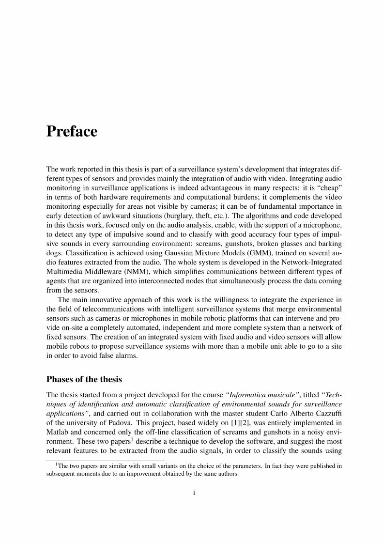
Preface
The work reported in this thesis is part of a surveillance system’s development that integrates dif-ferent types of sensors and provides mainly the integration of audio with video. Integrating audiomonitoring in surveillance applications is indeed advantageous in many respects: it is “cheap”in terms of both hardware requirements and computational burdens; it complements the videomonitoring especially for areas not visible by cameras; it can be of fundamental importance inearly detection of awkward situations (burglary, theft, etc.). The algorithms and code developedin this thesis work, focused only on the audio analysis, enable, with the support of a microphone,to detect any type of impulsive sound and to classify with good accuracy four types of impul-sive sounds in every surrounding environment: screams, gunshots, broken glasses and barkingdogs. Classification is achieved using Gaussian Mixture Models (GMM), trained on several au-dio features extracted from the audio. The whole system is developed in the Network-IntegratedMultimedia Middleware (NMM), which simplifies communications between different types ofagents that are organized into interconnected nodes that simultaneously process the data comingfrom the sensors.
The main innovative approach of this work is the willingness to integrate the experience inthe field of telecommunications with intelligent surveillance systems that merge environmentalsensors such as cameras or microphones in mobile robotic platforms that can intervene and pro-vide on-site a completely automated, independent and more complete system than a network offixed sensors. The creation of an integrated system with fixed audio and video sensors will allowmobile robots to propose surveillance systems with more than a mobile unit able to go to a sitein order to avoid false alarms.
Phases of the thesisThe thesis started from a project developed for the course “Informatica musicale”, titled “Tech-niques of identification and automatic classification of environmental sounds for surveillanceapplications”, and carried out in collaboration with the master student Carlo Alberto Cazzuffiof the university of Padova. This project, based widely on [1][2], was entirely implemented inMatlab and concerned only the off-line classification of screams and gunshots in a noisy envi-ronment. These two papers1 describe a technique to develop the software, and suggest the mostrelevant features to be extracted from the audio signals, in order to classify the sounds using
1The two papers are similar with small variants on the choice of the parameters. In fact they were published insubsequent moments due to an improvement obtained by the same authors.
i

GMMs. In our implementation we refer mostly to [2] because it was the last update regardingthis work.
The first phase of the project dealt with an implementation of the sound classification usingthe Matlab language, for the following reasons:
• simple and fast code programming;
• simple audio signals access from file .wav (functions wavread and wavwrite);
• GMM’s training algorithm already implemented in the Statistics Toolbox;
• availability of a Matlab tool that extracts 30 Mel-Frequency Cepstral Coefficients (MFCCs)and other features from an audio signal, developed by Enrico Marchetto, PhD student ofthe university of Padova.
In a second phase, when I decided to extend the work to my thesis, the code had to beimplemented in C++, in order to integrate it over the Network-Integrated Multimedia Middleware(NMM). For this reason, a long period of work has been devoted to porting all the code fromMatlab to C++, except for the GMM’s training algorithm and the audio test maker. The reasonwhy I choose not to port the GMM’s training algorithm is because the classification of the sounds(and of the environmental noise) can be made off-line, as well as the creation of the audio tests,and is compatible with a hypothetical product that does not require on-board training. The portingperiod lead fortunately to a strong optimization of the code, correction of some bugs/errors and afaster execution of the algorithm. In this period I introduced also two new classes of sounds withrespect to the initial project: broken glasses and barking dogs.
In the third period the attention switched to the porting of the software over the NMM archi-tecture following the suggestion of Prof. Emanuele Menegatti, who supervises a large projecton surveillance with many analytical nodes (audio and video). In collaboration with AlbertoSalamone, a master student of the University of Padova who realized a fall detector with an om-nidirectional camera and a steerable PTZ camera, I installed NMM and realized some processingnodes that can analyse and classify the recorded sound in real-time.
In the fourth and last period I assessed the performance of the audio classification in severalaspects, both on the off-line C++ implementation and on the real-time NMM realization.
Structure of the thesisThis thesis is structured in six chapters with an additional appendix. Chapter 1 reviews the stateof the art on this topic. In Chapter 2, all the mathematical tools used to realize and implement theclassification system are listed and explained. Chapter 3 contains the complete description of theoriginal work with project choices, and implementations. Chapter 4 is structured in three parts.The first part is a description of all the development tools used in the project. The second part iswritten as a “HowTo”guide to simplify the installation and configuration of the environment towork easily with the used middelware (NMM). The third part describes the implementation ofthe project in the middleware. All the experimental results are explained in Chapter 5, including
ii

both off-line and real-time tests. The final Chapter contains the conclusions of the work, aswell as further developments and hints suggested to improve the system. The appendix lists anddescribes all the libraries needed to install NMM.
iii

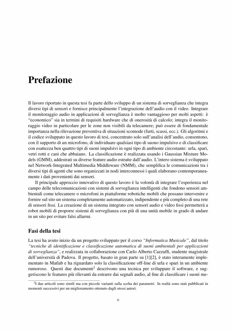
Prefazione
Il lavoro riportato in questa tesi fa parte dello sviluppo di un sistema di sorveglianza che integradiversi tipi di sensori e fornisce principalmente l’integrazione dell’audio con il video. Integrareil monitoraggio audio in applicazioni di sorveglianza e molto vantaggioso per molti aspetti: e“economico” sia in termini di requisiti hardware che di onerosita di calcolo; integra il monito-raggio video in particolare per le zone non visibili da telecamere; puo essere di fondamentaleimportanza nella rilevazione preventiva di situazioni scomode (furti, scassi, ecc.). Gli algoritmi eil codice sviluppato in questo lavoro di tesi, concentrato solo sull’analisi dell’audio, consentono,con il supporto di un microfono, di individuare qualsiasi tipo di suono impulsivo e di classificarecon esattezza ben quattro tipi di suoni impulsivi in ogni tipo di ambiente circostante: urla, spari,vetri rotti e cani che abbaiano. La classificazione e realizzata usando i Gaussian Mixture Mo-dels (GMM), addestrati su diverse feature audio estratte dall’audio. L’intero sistema e sviluppatonel Network-Integrated Multimedia Middleware (NMM), che semplifica le comunicazioni tra idiversi tipi di agenti che sono organizzati in nodi interconnessi i quali elaborano contemporanea-mente i dati provenienti dai sensori.
Il principale approccio innovativo di questo lavoro e la volonta di integrare l’esperienza nelcampo delle telecomunicazioni con sistemi di sorveglianza intelligenti che fondono sensori am-bientali come telecamere o microfoni in piattaforme robotiche mobili che possano intervenire efornire sul sito un sistema completamente automatizzato, indipendente e piu completo di una retedi sensori fissi. La creazione di un sistema integrato con sensori audio e video fissi permettera arobot mobili di proporre sistemi di sorveglianza con piu di una unita mobile in grado di andarein un sito per evitare falsi allarmi.
Fasi della tesiLa tesi ha avuto inizio da un progetto sviluppato per il corso “Informatica Musicale”, dal titolo“tecniche di identificazione e classificazione automatica di suoni ambientali per applicazionidi sorveglianza”, e realizzata in collaborazione con Carlo Alberto Cazzuffi, studente magistraledell’universita di Padova. Il progetto, basato in gran parte su [1][2], e stato interamente imple-mentato in Matlab e ha riguardato solo la classificazione off-line di urla e spari in un ambienterumoroso. Questi due documenti2 descrivono una tecnica per sviluppare il software, e sug-geriscono le features piu rilevanti da estrarre dai segnali audio, al fine di classificare i suoni me-
2I due articoli sono simili ma con piccole varianti sulla scelta dei parametri. In realta sono stati pubblicati inmomenti successivi per un miglioramento ottenuto dagli stessi autori.
v

diante GMM. Nella nostra implementazione ci riferiamo soprattutto a [2] perche e stato l’ultimoaggiornamento riguardante questo lavoro.
La prima fase del progetto ha riguardato l’implementazione della classificazione del suonoutilizzando il linguaggio Matlab per le seguenti ragioni:
• linguaggio di programmazione semplice e veloce;
• semplice accesso ai segnali audio da file .wav (con funzioni wavread e wavwrite);
• algoritmo di training delle GMM gia implementato nello Statistics Toolbox;
• disponibilita di un tool in Matlab che estrae 30 Mel-Frequency Cepstral Coefficients (MFCCs)e altre feature di un segnale audio, sviluppato da Enrico Marchetto, dottorando dell’Universitadi Padova.
In una seconda fase, quando ho deciso di estendere il lavoro alla mia tesi, si e verificato ilbisogno di implementare il codice in C++, al fine di integrarlo nel Network-Integrated Multime-dia Middleware (NMM). Per questo motivo, ho dedicato un lungo periodo di lavoro al portingdi tutto il codice da Matlab a C++, fatta eccezione per l’algoritmo di training dei GMM e ilprogramma per la creazione di test audio. Il motivo per cui ho scelto di non fare il portingdell’algoritmo di training dei GMM e perche la classificazione dei suoni (e del rumore ambien-tale) puo essere effettuata off-line, cosı come per la creazione dei test audio, ed e compatibilecon un ipotetico prodotto che non richiede il training on-board. Il periodo di porting ha portatofortunatamente ad una forte ottimizzazione del codice, alla correzione di alcuni bug/errori e aduna piu veloce esecuzione dell’algoritmo. In questo periodo ho introdotto anche due nuove classidi suoni rispetto al progetto iniziale: vetri rotti e cani che abbaiano.
Nel terzo periodo mi sono occupato del porting del software sull’architettura NMM seguendoil suggerimento del Prof. Emanuele Menegatti, che supervisiona un grande progetto sulla sorve-glianza con molti nodi analitici (audio e video). In collaborazione con Alberto Salamone, stu-dente magistrale dell’Universita di Padova che ha realizzato un rivelatore di caduta con unatelecamera omnidirezionale e una telecamera PTZ orientabile, ho installato NMM e realizzatoalcuni nodi di elaborazione in grado di analizzare e classificare il suono registrato in tempo reale.
Nel quarto e ultimo periodo ho testato le prestazioni della classificazione audio in parecchiaspetti, sia nell’implementazione off-line in C++ sia nella realizzazione in tempo reale in NMM.
Struttura della tesiQuesta tesi e strutturata in sei capitoli con un’appendice aggiuntiva. Il Capitolo 1 e la recen-sione dello stato dell’arte dell’argomento della tesi. Nel Capitolo 2 sono elencati e spiegati tuttigli strumenti matematici utilizzati per realizzare e implementare il sistema di classificazione. IlCapitolo 3 contiene la descrizione completa del lavoro originale con scelte progettuali e imple-mentazioni. Il Capitolo 4 e strutturato in tre parti. La prima parte e una descrizione di tutti glistrumenti di sviluppo utilizzati nel progetto. La seconda parte e scritta come una guida “HowTo”per semplificare l’installazione e la configurazione dell’ambiente per poter lavorare facilmente
vi

con il middelware utilizzato (NMM). La terza parte descrive l’implementazione del progetto nelmiddleware. Tutti i risultati sperimentali sono spiegati nel Capitolo 5, che include sia i test off-line che quelli in tempo reale. Il Capitolo finale contiene le conclusioni del lavoro, nonche gliulteriori sviluppi e spunti suggeriti per migliorare il sistema. L’appendice elenca e descrive tuttele librerie necessarie per installare NMM.
vii

Abstract
This thesis describes an audio event detection system which automatically classifies an impul-sive audio event as scream, gunshot, broken glasses or barking dogs with every backgroundnoise. The classification system uses four parallel Gaussian Mixture Models (GMMs) classifierseach of which decides if the sound belongs to its class or is only noise. Each classifier is trainedusing different features, chosen from a set of 40 audio features. Simultaneously the system candetect any kind of impulsive sounds using only one feature with very high precision. The clas-sification system is implemented in the Network-Integrated Multimedia Middleware (NMM) forreal-time processing and communications with other surveillance applications. In order to val-idate the proposed detection algorithm, we carried out extensive experiments (both off-line andreal-time) on a hand-made set of sounds mixed with ambient noise at different Signal-to-Noiseratios (SNRs). Our results demonstrate that the system is able to guarantee 70% of accuracy and90% of precision at 0 dB SNR, starting from 100% of both accuracy and precision with cleansounds at 20 dB SNR.
ix

Sommario
Questa tesi descrive un sistema di rilevazione di eventi audio che classifica automaticamente unrumore impulsivo come urla, spari, vetri rotti o cani che abbaiano con qualsiasi rumore di sot-tofondo. Il sistema di classificazione utilizza quattro classificatori in parallelo, costruiti con iGaussian Mixture Models (GMMs), ciascuno dei quali decide se il suono appartiene alla pro-pria classe o se e soltanto rumore. Ogni classificatore e addestrato con differenti feature, scelteda un insieme di 40 feature audio. Contemporaneamente il sistema puo rilevare qualsiasi tipodi suoni impulsivi utilizzando una sola feature con una precisione molto elevata. Il sistemadi classificazione e implementato nel Network-Integrated Multimedia Middleware (NMM) perl’elaborazione in tempo reale e le comunicazioni con altre applicazioni di sorveglianza. Al finedi validare l’algoritmo di rilevazione proposto, sono stati effettuati vari esperimenti (sia off-linesia in tempo reale) su un personale database di suoni, mescolati con rumore ambientale, a diversirapporti di segnale-rumore (SNR). I nostri risultati dimostrano che il sistema e in grado di garan-tire il 70% di accuratezza e il 90% di precisione a 0 dB di SNR, a partire da 100% di accuratezzae precisione con suoni puliti a 20 dB di SNR.
xi


AcknowledgementsFirst I want to thank my parents with a special hug, hoping that this goal would fill them withsatisfaction. I would like to thank my professors Federico Avanzini and Emanuele Menegatti tohelp me and direct my work in the right way. Special thanks go to Carlo Alberto Cazzuffi andAlberto Salamone that worked with me in this project and to Federica Ziliotto that helped meto correct the English version of this thesis. Thanks to Isacco Saccoman, author of the fabulouscomics in my final slide of the presentation. Acknowledgements go also to everyone that helpedand supported me directly or indirectly in my studies.
I sincerely apologize with Classical Music to have neglected it in order to finish my universitystudies.
xiii


RingraziamentiPrima di tutto vorrei ringraziare i miei genitori con un abbraccio speciale, sperando che questotraguardo li riempia di soddisfazione. Vorrei ringraziare i miei professori Federico Avanzinie Emanuele Menegatti per avermi aiutato e aver indirizzato il mio lavoro verso la direzionegiusta. Ringraziamenti particolari vanno a Carlo Alberto Cazzuffi e Alberto Salamone che hannolavorato con me in questo progetto e a Federica Ziliotto che mi ha aiutato a correggere la versionein inglese di questa tesi. Grazie a Isacco Saccoman, autore del favoloso fumetto nella slide finaledella mia presentazione. Ringraziamenti particolari vanno anche a tutti coloro che mi hannoaiutato e sostenuto direttamente o indirettamente durante i miei studi.
Mi scuso profondamente con la Musica Classica per averla trascurata per terminare i mieistudi universitari.
xv

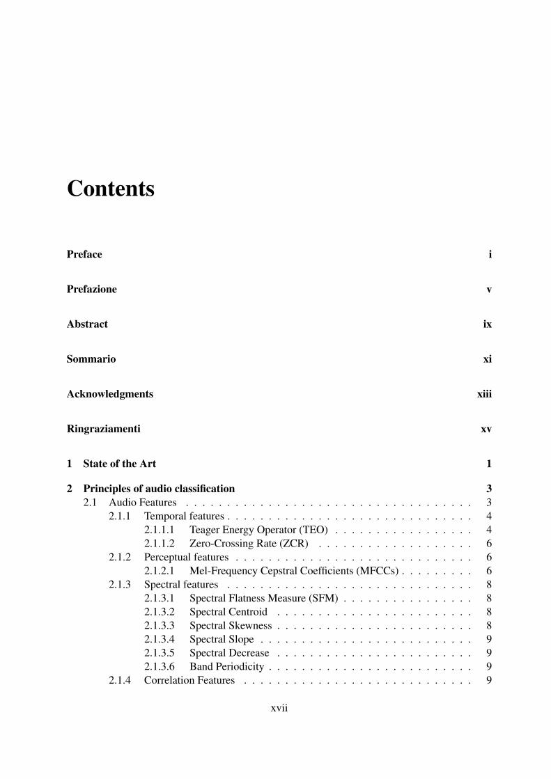
Contents
Preface i
Prefazione v
Abstract ix
Sommario xi
Acknowledgments xiii
Ringraziamenti xv
1 State of the Art 1
2 Principles of audio classification 32.1 Audio Features . . . . . . . . . . . . . . . . . . . . . . . . . . . . . . . . . . . 3
2.1.1 Temporal features . . . . . . . . . . . . . . . . . . . . . . . . . . . . . . 42.1.1.1 Teager Energy Operator (TEO) . . . . . . . . . . . . . . . . . 42.1.1.2 Zero-Crossing Rate (ZCR) . . . . . . . . . . . . . . . . . . . 6
2.1.2 Perceptual features . . . . . . . . . . . . . . . . . . . . . . . . . . . . . 62.1.2.1 Mel-Frequency Cepstral Coefficients (MFCCs) . . . . . . . . . 6
2.1.3 Spectral features . . . . . . . . . . . . . . . . . . . . . . . . . . . . . . 82.1.3.1 Spectral Flatness Measure (SFM) . . . . . . . . . . . . . . . . 82.1.3.2 Spectral Centroid . . . . . . . . . . . . . . . . . . . . . . . . 82.1.3.3 Spectral Skewness . . . . . . . . . . . . . . . . . . . . . . . . 82.1.3.4 Spectral Slope . . . . . . . . . . . . . . . . . . . . . . . . . . 92.1.3.5 Spectral Decrease . . . . . . . . . . . . . . . . . . . . . . . . 92.1.3.6 Band Periodicity . . . . . . . . . . . . . . . . . . . . . . . . . 9
2.1.4 Correlation Features . . . . . . . . . . . . . . . . . . . . . . . . . . . . 9
xvii
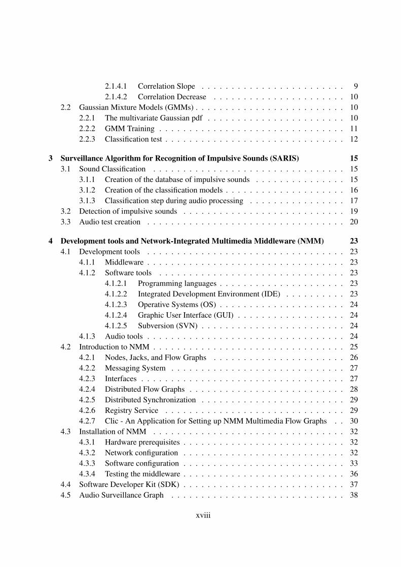
2.1.4.1 Correlation Slope . . . . . . . . . . . . . . . . . . . . . . . . 92.1.4.2 Correlation Decrease . . . . . . . . . . . . . . . . . . . . . . 10
2.2 Gaussian Mixture Models (GMMs) . . . . . . . . . . . . . . . . . . . . . . . . . 102.2.1 The multivariate Gaussian pdf . . . . . . . . . . . . . . . . . . . . . . . 102.2.2 GMM Training . . . . . . . . . . . . . . . . . . . . . . . . . . . . . . . 112.2.3 Classification test . . . . . . . . . . . . . . . . . . . . . . . . . . . . . . 12
3 Surveillance Algorithm for Recognition of Impulsive Sounds (SARIS) 153.1 Sound Classification . . . . . . . . . . . . . . . . . . . . . . . . . . . . . . . . 15
3.1.1 Creation of the database of impulsive sounds . . . . . . . . . . . . . . . 153.1.2 Creation of the classification models . . . . . . . . . . . . . . . . . . . . 163.1.3 Classification step during audio processing . . . . . . . . . . . . . . . . 17
3.2 Detection of impulsive sounds . . . . . . . . . . . . . . . . . . . . . . . . . . . 193.3 Audio test creation . . . . . . . . . . . . . . . . . . . . . . . . . . . . . . . . . 20
4 Development tools and Network-Integrated Multimedia Middleware (NMM) 234.1 Development tools . . . . . . . . . . . . . . . . . . . . . . . . . . . . . . . . . 23
4.1.1 Middleware . . . . . . . . . . . . . . . . . . . . . . . . . . . . . . . . . 234.1.2 Software tools . . . . . . . . . . . . . . . . . . . . . . . . . . . . . . . 23
4.1.2.1 Programming languages . . . . . . . . . . . . . . . . . . . . . 234.1.2.2 Integrated Development Environment (IDE) . . . . . . . . . . 234.1.2.3 Operative Systems (OS) . . . . . . . . . . . . . . . . . . . . . 244.1.2.4 Graphic User Interface (GUI) . . . . . . . . . . . . . . . . . . 244.1.2.5 Subversion (SVN) . . . . . . . . . . . . . . . . . . . . . . . . 24
4.1.3 Audio tools . . . . . . . . . . . . . . . . . . . . . . . . . . . . . . . . . 244.2 Introduction to NMM . . . . . . . . . . . . . . . . . . . . . . . . . . . . . . . . 25
4.2.1 Nodes, Jacks, and Flow Graphs . . . . . . . . . . . . . . . . . . . . . . 264.2.2 Messaging System . . . . . . . . . . . . . . . . . . . . . . . . . . . . . 274.2.3 Interfaces . . . . . . . . . . . . . . . . . . . . . . . . . . . . . . . . . . 274.2.4 Distributed Flow Graphs . . . . . . . . . . . . . . . . . . . . . . . . . . 284.2.5 Distributed Synchronization . . . . . . . . . . . . . . . . . . . . . . . . 294.2.6 Registry Service . . . . . . . . . . . . . . . . . . . . . . . . . . . . . . 294.2.7 Clic - An Application for Setting up NMM Multimedia Flow Graphs . . 30
4.3 Installation of NMM . . . . . . . . . . . . . . . . . . . . . . . . . . . . . . . . 324.3.1 Hardware prerequisites . . . . . . . . . . . . . . . . . . . . . . . . . . . 324.3.2 Network configuration . . . . . . . . . . . . . . . . . . . . . . . . . . . 324.3.3 Software configuration . . . . . . . . . . . . . . . . . . . . . . . . . . . 334.3.4 Testing the middleware . . . . . . . . . . . . . . . . . . . . . . . . . . . 36
4.4 Software Developer Kit (SDK) . . . . . . . . . . . . . . . . . . . . . . . . . . . 374.5 Audio Surveillance Graph . . . . . . . . . . . . . . . . . . . . . . . . . . . . . 38
xviii

5 Experimental Results 435.1 Testing Off-line . . . . . . . . . . . . . . . . . . . . . . . . . . . . . . . . . . . 43
5.1.1 Global classification performance . . . . . . . . . . . . . . . . . . . . . 455.1.2 Single class classification performance . . . . . . . . . . . . . . . . . . 46
5.1.2.1 Gunshots . . . . . . . . . . . . . . . . . . . . . . . . . . . . . 475.1.2.2 Screams . . . . . . . . . . . . . . . . . . . . . . . . . . . . . 495.1.2.3 Broken Glasses . . . . . . . . . . . . . . . . . . . . . . . . . 515.1.2.4 Barking dogs . . . . . . . . . . . . . . . . . . . . . . . . . . . 53
5.2 Testing Real-time . . . . . . . . . . . . . . . . . . . . . . . . . . . . . . . . . . 555.2.1 Classification performance . . . . . . . . . . . . . . . . . . . . . . . . . 555.2.2 Impulse detection performance . . . . . . . . . . . . . . . . . . . . . . . 55
6 Conclusions and further work 57
Appendix 61
A Libraries for the installation of NMM 61A.1 Informations on external libraries . . . . . . . . . . . . . . . . . . . . . . . . . . 63
A.1.1 a52dec . . . . . . . . . . . . . . . . . . . . . . . . . . . . . . . . . . . 63A.1.2 faad . . . . . . . . . . . . . . . . . . . . . . . . . . . . . . . . . . . . . 64A.1.3 ffmpeg . . . . . . . . . . . . . . . . . . . . . . . . . . . . . . . . . . . 64A.1.4 I1394 . . . . . . . . . . . . . . . . . . . . . . . . . . . . . . . . . . . . 66A.1.5 libmp3lame . . . . . . . . . . . . . . . . . . . . . . . . . . . . . . . . . 66A.1.6 libraw1394 . . . . . . . . . . . . . . . . . . . . . . . . . . . . . . . . . 67A.1.7 libmad . . . . . . . . . . . . . . . . . . . . . . . . . . . . . . . . . . . 67A.1.8 libdvdnav . . . . . . . . . . . . . . . . . . . . . . . . . . . . . . . . . . 67A.1.9 libdvdread . . . . . . . . . . . . . . . . . . . . . . . . . . . . . . . . . 68A.1.10 libogg . . . . . . . . . . . . . . . . . . . . . . . . . . . . . . . . . . . . 68A.1.11 libvorbis . . . . . . . . . . . . . . . . . . . . . . . . . . . . . . . . . . 69A.1.12 libshout . . . . . . . . . . . . . . . . . . . . . . . . . . . . . . . . . . . 69A.1.13 fftw . . . . . . . . . . . . . . . . . . . . . . . . . . . . . . . . . . . . . 70A.1.14 libliveMedia . . . . . . . . . . . . . . . . . . . . . . . . . . . . . . . . 70A.1.15 mpeg2dec . . . . . . . . . . . . . . . . . . . . . . . . . . . . . . . . . . 71A.1.16 cdparanoia . . . . . . . . . . . . . . . . . . . . . . . . . . . . . . . . . 72A.1.17 libpng . . . . . . . . . . . . . . . . . . . . . . . . . . . . . . . . . . . . 72A.1.18 asoundlib . . . . . . . . . . . . . . . . . . . . . . . . . . . . . . . . . . 72A.1.19 Xlib . . . . . . . . . . . . . . . . . . . . . . . . . . . . . . . . . . . . . 73A.1.20 libjpeg . . . . . . . . . . . . . . . . . . . . . . . . . . . . . . . . . . . 73A.1.21 ImageMagick . . . . . . . . . . . . . . . . . . . . . . . . . . . . . . . . 73A.1.22 ImageMagick for Windows . . . . . . . . . . . . . . . . . . . . . . . . . 74A.1.23 mplayer . . . . . . . . . . . . . . . . . . . . . . . . . . . . . . . . . . . 74A.1.24 vlc . . . . . . . . . . . . . . . . . . . . . . . . . . . . . . . . . . . . . . 74A.1.25 transcode . . . . . . . . . . . . . . . . . . . . . . . . . . . . . . . . . . 75
xix

A.1.26 ogmtools . . . . . . . . . . . . . . . . . . . . . . . . . . . . . . . . . . 75A.1.27 libxml++ . . . . . . . . . . . . . . . . . . . . . . . . . . . . . . . . . . 75A.1.28 libx264 . . . . . . . . . . . . . . . . . . . . . . . . . . . . . . . . . . . 76A.1.29 DVB API 5.1 . . . . . . . . . . . . . . . . . . . . . . . . . . . . . . . . 76A.1.30 ulxmlrpcpp . . . . . . . . . . . . . . . . . . . . . . . . . . . . . . . . . 76A.1.31 openssl . . . . . . . . . . . . . . . . . . . . . . . . . . . . . . . . . . . 77A.1.32 expat . . . . . . . . . . . . . . . . . . . . . . . . . . . . . . . . . . . . 77
xx
List of Figures
2.1 Signal with four impulsive sounds and his TEO. . . . . . . . . . . . . . . . . . . 52.2 Plots of pitch mels versus hertz. . . . . . . . . . . . . . . . . . . . . . . . . . . 72.3 Generic data distribution generated from a mixture of four bivariate Gaussian
distributions. . . . . . . . . . . . . . . . . . . . . . . . . . . . . . . . . . . . . 122.4 Estimated probability density contours for the distribution with various values of
the number of the components k. . . . . . . . . . . . . . . . . . . . . . . . . . . 13
3.1 Visualization of likelihood and detection in time. The upper plot is the detectionover the time and in the other plots there are the values of the likelihood of eachmodel. Legend: black - impulsive sound; red - gunshots; green - screams; blue -broken glasses; light blue - barking dogs. . . . . . . . . . . . . . . . . . . . . . 21
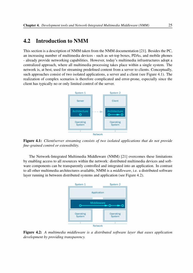
4.1 Client/server streaming consists of two isolated applications that do not providefine-grained control or extensibility. . . . . . . . . . . . . . . . . . . . . . . . . 25
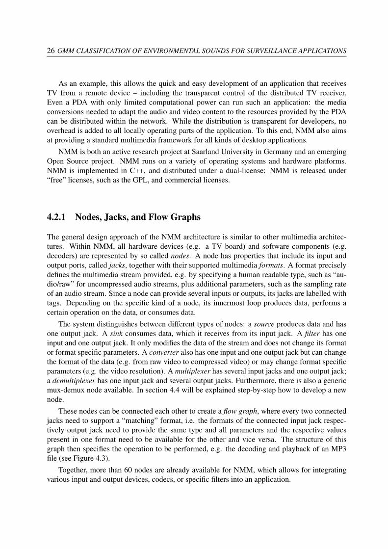
4.2 A multimedia middleware is a distributed software layer that eases applicationdevelopment by providing transparency. . . . . . . . . . . . . . . . . . . . . . . 25
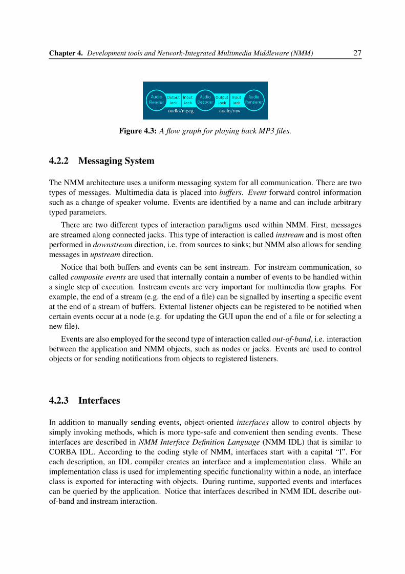
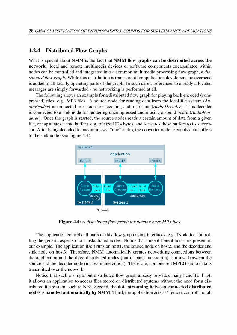
4.3 A flow graph for playing back MP3 files. . . . . . . . . . . . . . . . . . . . . . . 274.4 A distributed flow graph for playing back MP3 files. . . . . . . . . . . . . . . . . 284.5 The Audio Surveillance Graph. . . . . . . . . . . . . . . . . . . . . . . . . . . . 39
5.1 High accuracy but low precision. . . . . . . . . . . . . . . . . . . . . . . . . . . 445.2 High precision but low accuracy. . . . . . . . . . . . . . . . . . . . . . . . . . . 445.3 Accuracy of all the classes. . . . . . . . . . . . . . . . . . . . . . . . . . . . . . 455.4 Precision of all the classes. . . . . . . . . . . . . . . . . . . . . . . . . . . . . . 465.5 Accuracy of the Gunshot class with simple validation. . . . . . . . . . . . . . . . 475.6 Precision of the Gunshot class with simple validation. . . . . . . . . . . . . . . . 475.7 Accuracy of the Gunshot class with LOOCV. . . . . . . . . . . . . . . . . . . . 485.8 Precision of the Gunshot class with LOOCV. . . . . . . . . . . . . . . . . . . . 485.9 Accuracy of the Scream class with simple validation. . . . . . . . . . . . . . . . 495.10 Precision of the Scream class with simple validation. . . . . . . . . . . . . . . . 495.11 Accuracy of the Scream class with LOOCV. . . . . . . . . . . . . . . . . . . . . 505.12 Precision of the Scream class with LOOCV. . . . . . . . . . . . . . . . . . . . . 505.13 Accuracy of the Broken Glasses class with simple validation. . . . . . . . . . . . 515.14 Precision of the Glass class with simple validation. . . . . . . . . . . . . . . . . 51
xxi

5.15 Accuracy of the Glass class with LOOCV. . . . . . . . . . . . . . . . . . . . . . 525.16 Precision of the Glass class with LOOCV. . . . . . . . . . . . . . . . . . . . . . 525.17 Accuracy of the Barking dogs class with simple validation. . . . . . . . . . . . . 535.18 Precision of the Bark class with simple validation. . . . . . . . . . . . . . . . . . 535.19 Accuracy of the Bark class with LOOCV. . . . . . . . . . . . . . . . . . . . . . 545.20 Precision of the Bark class with LOOCV. . . . . . . . . . . . . . . . . . . . . . 54
xxii

List of Tables
3.1 Number of files and total duration in seconds for each audio sound class. . . . . . 163.2 Features selected to create the Gaussian Mixture Models. . . . . . . . . . . . . . 163.3 Thresholds and the lengths of the windows used for selecting the likelihood of
the sounds for detection. . . . . . . . . . . . . . . . . . . . . . . . . . . . . . . 193.4 Threshold and the length of the windows used for selecting the TEO-signal of
the sound. . . . . . . . . . . . . . . . . . . . . . . . . . . . . . . . . . . . . . . 20
xxiii

Chapter 1
State of the Art
In addition to the traditional video cameras, the use of audio sensors in surveillance and monitor-ing applications is becoming increasingly important [3]. Audio is useful especially in situationswhen other sensors, such as video, fails to detect correctly the events. For example, when objectsare occluded or in the dark, audio sensors can be more appropriate in detecting a “noisy” pres-ence. Conceptually, there are many events which can be detected better using audio rather thanother sensors, e.g. screams or gunshots [4][5], broken glasses, barking dogs, etc. Furthermore,audio sensors are a quite accessible resource for the costs.
Such detection systems can be efficiently used to advert an automated system that an eventhas occurred with high probability and, at the same time, to enable further processing like auto-matic video-camera steering. Traditional tasks in the area of the automatic audio classificationand matching are speech/music segmentation, classification and audio retrieval. Much of the pre-vious work about audio-based surveillance systems concentrated on the task of detecting someparticular audio events. More recently, were developed specific works covering the detection ofparticular classes of events for multimedia-based surveillance. For example, detection systemsspecifically designed for impulsive sound1 recognition consist of a segmentation step, where isdetected the presence of an event, followed by a classification step, which refines the result as-signing a class label to the event. The results reported in [6], show that these systems fail underreal-world conditions reaching less than 50% accuracy at 0 dB SNR (Signal-to-Noise Ratio).
Mel-Frequency Cepstral Coefficients (MFCCs) are the most common features representationfor non-speech audio recognition. Peltonen et al. in [7] implemented a system for recogniz-ing 17 sound events using 11 features individually and obtained best results with the MFCCs.In a comparison of several feature sets, MFCCs perform well [8], although the classificationgranularity affects the relative importance of different feature sets. Cai et al. in [9] used a com-bination of statistical features and labels describing the energy envelope, harmonicity, and pitchcontour for each sample. None of these representations, unfortunately, shows clear performanceor conceptual advantages over MFCCs.
In the SOLAR system presented in [10], the segmentation step is avoided by decomposing
1A definition of impulsive sound is a sound with a rapid rise and decay of sound pressure level, lasting less thanone second. It is caused by sudden contact between two or more surfaces or by a sudden release of pressure. Inother words it is a sound that makes you turn your head and open your ears putting your body in an “alarm” state.
1
2 GMM CLASSIFICATION OF ENVIRONMENTAL SOUNDS FOR SURVEILLANCE APPLICATIONS
audio tracks into short overlapping audio windows. For each window, a set of 138 featuresis extracted and evaluated by a series of boosted decision trees. Though efficient in real timecomputations, the SOLAR system suffers from large differences in classification accuracy fromclass to class. More recent works showed that a hierarchical classification scheme, composedby different levels of binary classifiers, generally achieves higher performance than a single-level multi-class classifier. In [11] a hierarchical set of cascaded GMMs (Gaussian MixtureModels) is used to classify 5 different sound classes. Each GMM is tuned using only one featurefrom a feature set including both scalar features (e.g. Zero-Crossing Rate (ZCR)) or vectorfeatures (e.g. Linear-Log Frequency Cepstral Coefficients (LLFCC)). Reported results show thatthe hierarchical approach yields accuracies from 70 to 80% for each class, while single levelapproaches reach high accuracies for one class but poor results for the others.
The hierarchical approach has also been employed in [4] to design a specific system able todetect screams/shouts in public transport environments. After a preliminary segmentation step,a set of perceptual features such as MFCCs or Perceptual Linear Prediction (PLP) coefficientsare extracted from audio segments and used to perform a 3-levels classification. First, the au-dio segment is classified either as noise or non-noise; second, if it is not noise, the segment isclassified either as speech or not speech; finally, if speech, it is classified as a shout or not. Theauthors tested this system using both GMMs and Support Vector Machines (SVMs) as classifiers,showing that generally GMMs provide higher precision.
A different technique is used in [5] to detect gunshots in public environments. In this work,the performance of a binary gunshot/noise GMM classifier is compared to a classification schemein which several binary sub classifiers for different types of firearms run in parallel. A final binarydecision (gunshot/noise) is taken evaluating the logical OR of the results of each classifier. Inthis way, the false rejection rate of the system is reduced by a 50% on average with respect to theoriginal binary classifier.
In a recent work [1][2], Valenzise et al. proposed a system that is able to detect accurately twotypes of audio events: screams and gunshots. They extract a very large set of features, includingsome descriptors like spectral slope and periodicity, and innovative features like correlation roll-off and decrease. To the authors knowledge, these features have never been used for the task ofsound-based surveillance and it is shown that they provide a significant performance gain usinga GMM as classifier.
The current project is a deep study and elaboration of the works [1][2] and can be seen asan implementation and improvement of them. This work is different from the previous ones inthe following aspects. First, to manage a multimedia surveillance system and synchronize allprocesses of sensors and agents, is used NMM (Network-Integrated Multimedia Middleware).Second, the system can detect any kind of impulsive sound, with only one feature, using only asingle microphone data with very high precision. Finally, over the screams and gunshots impul-sive sound classes, the system can detect and classify even broken glasses and barking dogs.
Chapter 2
Principles of audio classification
In this chapter we describe the main mathematical tools used in the project to introduce the readerto the main topics of the thesis.
2.1 Audio FeaturesA considerable number of audio features was used in the project. Traditionally, these featuresare classified in:
• Temporal features - e.g. Teager Energy Operator (TEO) or Zero-Crossing Rate (ZCR);
• Perceptual features - e.g. loudness, sharpness or Mel-Frequency Cepstral Coefficients(MFCCs);
• Energy features - e.g. Short Time Energy (STE);
• Spectral features - e.g. spectral flatness, spectral skewness;
In this work are discarded the audio features which are too sensitive to the SNR conditions,like STE and loudness. In addition to the traditional features listed above, are employed someother features which have been introduced in [1][2], such as spectral distribution (spectral slope,spectral decrease), periodicity descriptors and new features based on the auto-correlation func-tion: correlation decrease and correlation slope. The number of features extracted is 41 and arethe following:
• Teager Energy Operator (TEO);
• Zero Crossing Rate (ZCR);
• 30 Mel-Frequency Cepstral Coefficients (MFCCs);
• Spectral Flatness Measure (SFM);
3
4 GMM CLASSIFICATION OF ENVIRONMENTAL SOUNDS FOR SURVEILLANCE APPLICATIONS
• Spectral Centroid;
• Spectral Skewness;
• Spectral Slope;
• Spectral Decrease;
• Whole-Band Periodicity;
• Filtered-Band Periodicity;
• Correlation Slope;
• Correlation Decrease.
Now it follows a detailed definition of all the features used in the project. Note that an audioframe is a small audio segment of the whole audio signal. In other words, a frame is a fixed-length array containing a part of the values of the audio signal. TEO will be used to detect ageneric impulsive sound and all other features will be used for the classification of the impulsivesounds.
2.1.1 Temporal features2.1.1.1 Teager Energy Operator (TEO)
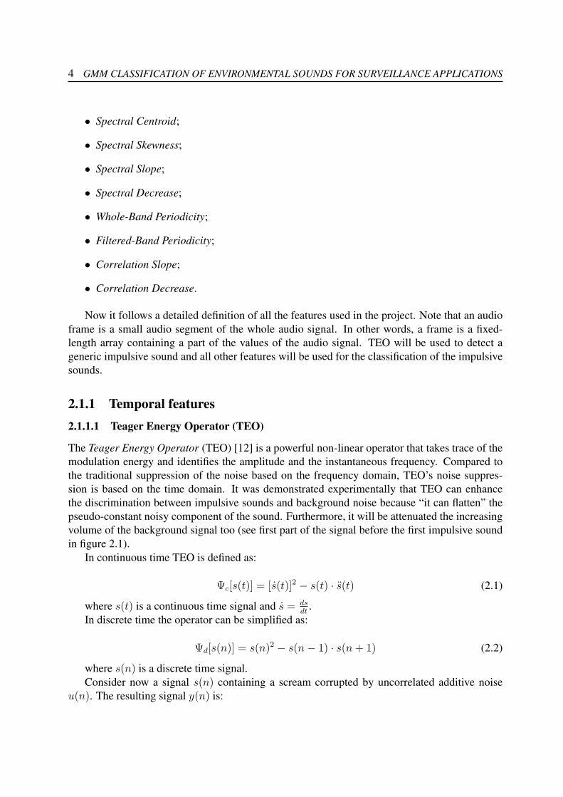
The Teager Energy Operator (TEO) [12] is a powerful non-linear operator that takes trace of themodulation energy and identifies the amplitude and the instantaneous frequency. Compared tothe traditional suppression of the noise based on the frequency domain, TEO’s noise suppres-sion is based on the time domain. It was demonstrated experimentally that TEO can enhancethe discrimination between impulsive sounds and background noise because “it can flatten” thepseudo-constant noisy component of the sound. Furthermore, it will be attenuated the increasingvolume of the background signal too (see first part of the signal before the first impulsive soundin figure 2.1).
In continuous time TEO is defined as:
Ψc[s(t)] = [s(t)]2 − s(t) · s(t) (2.1)
where s(t) is a continuous time signal and s = dsdt
.In discrete time the operator can be simplified as:
Ψd[s(n)] = s(n)2 − s(n− 1) · s(n+ 1) (2.2)
where s(n) is a discrete time signal.Consider now a signal s(n) containing a scream corrupted by uncorrelated additive noise
u(n). The resulting signal y(n) is:
Chapter 2. Principles of audio classification 5
0 1 2 3 4 5 6 7 8 9
x 105
−1
−0.5
0
0.5
1
Samples
Am
plitu
de
Signal − s(n)
0 1 2 3 4 5 6 7 8 9
x 105
−0.2
0
0.2
0.4
0.6
0.8
Samples
Am
plitu
de
Teager − TEO[s(n)]
Figure 2.1: Signal with four impulsive sounds and his TEO.
y(n) = s(n) + u(n) (2.3)
Let Ψs[y(n)] the TEO of the signal y(n). It is defined as:
Ψd[y(n)] = Ψd[s(n)] + Ψd[u(n)] + 2 · Ψd[s(n), u(n)] (2.4)
where Ψd[s(n)] and Ψd[u(n)] are the TEO of the scream and of the additive noise respectively.Let Ψd[s(n), u(n)] the mutual energy Ψd between s(n) and u(n) such that:
Ψd[s(n), u(n)] = s(n) · u(n)− 0.5 · s(n− 1) · u(n+ 1) + 0.5 · s(n+ 1) ◦ u(n− 1) (2.5)
where ◦ represents the inner product.As the signals s(n) and u(n) have zero mean and are uncorrelated, the expected value of the
mutual energy Ψd[s(n), u(n)], is zero. So it is possible to obtain the following equation:
E{Ψd[y(n)]} = E{Ψd[s(n)]}+ E{Ψd[u(n)]} (2.6)
6 GMM CLASSIFICATION OF ENVIRONMENTAL SOUNDS FOR SURVEILLANCE APPLICATIONS
In fact, TEO of the scream is significantly higher than TEO of the noise. So, compared toE{Ψd[y(n)]}, the expected value E{Ψd[u(n)]} is irrelevant. Finally we obtain the relation:
E{Ψd[y(n)]} ≈ E{Ψd[s(n)]} (2.7)
2.1.1.2 Zero-Crossing Rate (ZCR)
ZCR is the rate of sign-changes along a signal [13]. In other words it is a measure of times’number the signal value crosses the zero axis rated by the number of values of the signal. Periodicsounds tend to have small ZCR, while noisy sounds tend to have high ZCR. The formula is:
ZCR =1
N − 1·N−1∑n=1
π(s(n) · s(n− 1) < 0) (2.8)
where s is a signal of length N and the function π(x) is 1 if its argument x is True and 0otherwise.
2.1.2 Perceptual features2.1.2.1 Mel-Frequency Cepstral Coefficients (MFCCs)
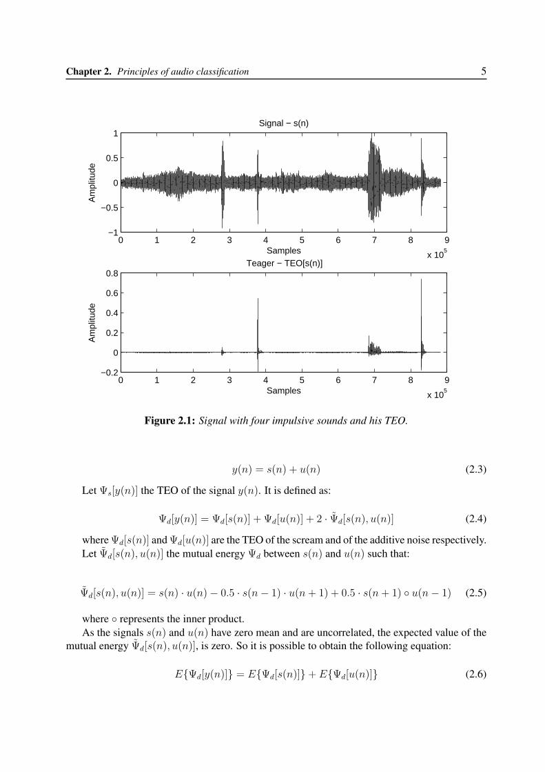
The mel scale, proposed by Stevens, Volkman and Newman in 1937 [14], is a perceptual scaleof pitches judged by listeners to be equal in distance from one another. The reference pointbetween this scale and normal frequency measurement is defined by equating a 1000 Hz tone,40 dB above the listener’s threshold, with a pitch of 1000 mels. Above about 500 Hz, largerand larger intervals are judged by listeners to produce equal pitch increments. As a result, fouroctaves on the hertz scale above 500 Hz are judged to comprise about two octaves on the melscale (see Figure 2.2). The name mel comes from the word melody to indicate that the scale isbased on pitch comparisons.
A popular formula to convert f hertz into m mel is1:
m = 2595 log10
(f
700+ 1
)= 1127 loge
(f
700+ 1
)(2.9)
And the inverse:
f = 700(10m/2595 − 1) = 700(em/1127 − 1) (2.10)
The mel-frequency cepstrum (MFC) is a representation of the short-term power spectrum ofa sound, based on a linear cosine transform of a log power spectrum on a non-linear mel scale offrequency.
1The base-10 formula with 2595 is from O’Shaughnessy (1987) [15]. The natural-log formula with coefficient1127 is widely used more recently. Older publications typically use the break frequency of 1000 Hz rather than 700Hz.
Chapter 2. Principles of audio classification 7
Figure 2.2: Plots of pitch mels versus hertz.
MFCCs collectively make up an MFC [13]. They are derived from a type of cepstral repre-sentation of the audio clip (a non-linear “spectrum-of-a-spectrum”). In the MFC the frequencybands are equally spaced on the mel scale, which approximates the human auditory system’sresponse more closely than the linearly-spaced frequency bands used in the normal cepstrum. Infact MFCC reflects the energy distribution over the basilar membrane. Due to their perceptuallymotivated nature, MFCCs are considered to carry a high amount of relevant information relatedto a sound signal. In fact they are often used to characterize a sound signal in such applications asautomatic speech/speaker recognition, and are increasingly used in music information retrievalapplications too [16].
The MFCCs are derived as follows:
1. take the Fourier transform of a frame of a signal;
2. map the powers of the spectrum obtained above onto the mel scale, using triangular over-lapping windows;
3. take the log of the powers at each of the mel frequencies;
4. take the discrete cosine transform of the list of mel log powers, as if it were a signal;
5. the MFCCs are the amplitudes of the resulting spectrum.
In the present project we extract 30 MFCCs as in [1][2].
8 GMM CLASSIFICATION OF ENVIRONMENTAL SOUNDS FOR SURVEILLANCE APPLICATIONS
2.1.3 Spectral features
2.1.3.1 Spectral Flatness Measure (SFM)
SFM is a measure used in digital signal processing to characterize an audio spectrum [13]. Highspectral flatness indicates that the spectrum has a similar amount of power in all spectral bandsand this would sounds similar to white noise. Low spectral flatness, instead, indicates that thespectral power is concentrated in a relatively small number of bands and it is typical for tonalsounds.
The spectral flatness is calculated by dividing the geometric mean of the power spectrum bythe arithmetic mean of the power spectrum. The spectral flatness used is measured across thewhole band.
SFM =
N
√∏N−1n=0 x(n)∑N−1
n=0 x(n)
N
(2.11)
where x(n) represents the magnitude of bin number n of the power spectrum.
2.1.3.2 Spectral Centroid
Spectral centroid is a measure that indicates where is the “center of mass” of the spectrum [13].Perceptually, it has a robust connection with the impression of “brightness” of a sound. It iscalculated as the weighted mean of the frequencies present in the frame, determined using aFourier transform, with their magnitudes as weights:
Centroid =
∑N−1n=0 f (n) · x (n)∑N−1
n=0 x (n)(2.12)
where x(n) represents the weighted frequency value, or magnitude, of bin number n, andf(n) represents the center frequency of that bin.
2.1.3.3 Spectral Skewness
Spectral skewness is a measure of the asymmetry of the probability distribution of a real-valuedrandom variable that in this context is the spectrum of the signal [13]. The skewness value canbe positive or negative, or even zero. Qualitatively, a negative skew indicates that the tail on theleft side of probability density function is longer than the right side and the bulk of the values(including the median) lies to the right of the mean. A positive skew indicates that the tail onthe right side is longer than the left side and the bulk of the values lies to the left of the mean.A zero value indicates that the values are relatively evenly distributed on both sides of the mean,typically but not necessarily implying a symmetric distribution.
For a sample of N values forming a frame, the skewness is:
Chapter 2. Principles of audio classification 9
Skewness =m3
m3/22
=1N·∑N−1
n=0 (x(n)− x)3(1N·∑N−1
n=0 (x(n)− x)2)3/2
(2.13)
where x represents the mean of the magnitudes, m3 is the sample third central moment, andm2 is the sample variance.
2.1.3.4 Spectral Slope
Spectral slope represents the amount of decreasing of the spectral amplitude [13]. It is computedby linear regression of the spectral amplitude. In other words it is the slope of the line-of-best-fitthrough the spectral data.
2.1.3.5 Spectral Decrease
Spectral decrease also represents the amount of decreasing of the spectral amplitude. This for-mulation comes from perceptual studies and it is supposed to be more correlated to human per-ception. The formula is:
Decrease =1∑N−1
n=1 x(n)·N−1∑n=1
x(n)− x(0)
N − 1(2.14)
where x(n) represents the weighted frequency value, or magnitude, of bin number n.
2.1.3.6 Band Periodicity
Band periodicity is defined in [17] as the periodicity of a sub band and can be derived by subband correlation analysis. In the current project it was chosen to use two different bands: thefirst one goes from 300 to 2500 Hz (called Filtered-Band Periodicity), the second one is from 0to 22050 Hz (called Whole-Band Periodicity) as suggested in [1][2]. The periodicity property ofeach sub band is represented by the maximum local peak of the normalized correlation functioncalculated from the current frame and previous frame.
2.1.4 Correlation Features
These features are similar to spectral distribution descriptors but, in lieu of the spectrogram, theyare computed starting from the auto-correlation function of each frame of the audio signal.
2.1.4.1 Correlation Slope
This feature is calculated giving the auto-correlation function of each frame of the audio signalas input to the slope function.
10 GMM CLASSIFICATION OF ENVIRONMENTAL SOUNDS FOR SURVEILLANCE APPLICATIONS
2.1.4.2 Correlation Decrease
This feature is calculated giving the auto-correlation function of each frame of the audio signalas input to the decrease function.
2.2 Gaussian Mixture Models (GMMs)Gaussian Mixture Models (GMMs) are among the most statistically mature methods for clus-tering [18] and are gaining increasing attention in the pattern recognition community. GMMsare widely used in audio applications like speaker recognition and music classification. GMM isan unsupervised classifier which means that the training samples of a classifier are not labelledto show their category membership. More precisely, what makes GMM unsupervised is thatduring the training of the classifier, we try to estimate the underlying probability density func-tions (pdf’s) of the observations. GMM can be classified as a semi-parametric density estimationmethod too, since it defines a very general class of functional forms for the density model. Inthis mixture model, a probability density function is expressed as a linear combination of basisfunctions. An interesting property of GMMs is that the training procedure is done indepen-dently for the classes by constructing a Gaussian mixture for each given class separately. So,adding a new class to a classification problem does not require retraining the whole system anddoes not affect the topology of the classifier making it attractive for pattern recognition applica-tions. While GMM provides very good performances and interesting properties as a classifier, itpresents some problems that may limit its practical use in real-time applications. One problemis that a GMM can require large amounts of memory to store various coefficients and complexcomputations mainly involving exponential calculations.
2.2.1 The multivariate Gaussian pdfIn the GMM classifier, the conditional-pdf of the observation vector is modeled as a linear com-bination of multivariate Gaussian pdfs, each of them with the following general form:
p(x) =1
(2π)d2 · |Σ|2
e{−12(x−µ)TΣ−1(x−µ)} (2.15)
where :
• d is the number of features in the model;
• x is a d-component feature vector;
• µ is the d-component vector containing the mean of each feature;
• Σ is the d-by-d covariance matrix and |Σ| is its determinant. It characterizes the dispersionof the data on the d-dimensions for the feature vector. The diagonal element σii is thevariance of xi and the non diagonal elements are the covariances between features. Often
Chapter 2. Principles of audio classification 11
the assumption is that the features are independent, so Σ is diagonal and p(x) can actuallybe written as the product of the univariate probability densities for the elements of x.
It is important to note that each multivariate Gaussian pdf is completely defined if we knowθ = [µ,Σ].
2.2.2 GMM TrainingTo classify data using features vectors in a class, GMM needs a training step. At this stage, wehave to estimate the parameters of the multivariate Gaussian pdfs: θi = [µi,Σi] with i = 1, . . . , kand k the number of multivariate Gaussian pdfs. In literature, the Expectation-Maximizationalgorithm (EM) is the most often used solution for this problem. EM is an iterative methodwhich starts from a random distribution and alternates between performing an expectation (E)step, which computes the expectation of the log-likelihood evaluated using the current estimatefor the latent variables, and a maximization (M) step, which computes parameters maximizingthe expected log-likelihood found on the E step. These parameter-estimates are then used todetermine the distribution of the latent variables in the next E step. This algorithm is assured toconverge to a local optimum. Note that the training set provided to GMM has to be well thoughtout in order to have a model to be general enough to avoid the common problem of overfitting.
A simple Matlab example with real data will explain better the argument. To demonstrate theprocess, first generate some simulated data from a mixture of four bivariate Gaussian distribu-tions using the mvnrnd function2 (see Figure 2.3).
mu1 = [1 2];sigma1 = [3 0.2; 0.2 2];mu2 = [-1 -2];sigma2 = [2 0; 0 1];mu3 = [-4 2];sigma3 = [1 0; 0 1];mu4 = [-6 -2];sigma4 = [2 -1; -1 2];
X = [mvnrnd(mu1,sigma1,100); mvnrnd(mu2,sigma2,100);mvnrnd(mu3,sigma3,100); mvnrnd(mu4,sigma4,100)];scatter(X(:,1),X(:,2),10,’ok’)
Now we have to fit the data with the GMM training algorithm. Here, we know that thecorrect number of components to use is k = 4. Actually, with real data, this decision wouldrequire comparing models with different number of components.
gm = gmdistribution.fit(X,k);
2Here we assume that all data belong to the same class and are independent each other, even if they are not,simply to have a generic data distribution.

12 GMM CLASSIFICATION OF ENVIRONMENTAL SOUNDS FOR SURVEILLANCE APPLICATIONS
−10 −5 0 5−6
−4
−2
0
2
4
6
Figure 2.3: Generic data distribution generated from a mixture of four bivariate Gaussian dis-tributions.
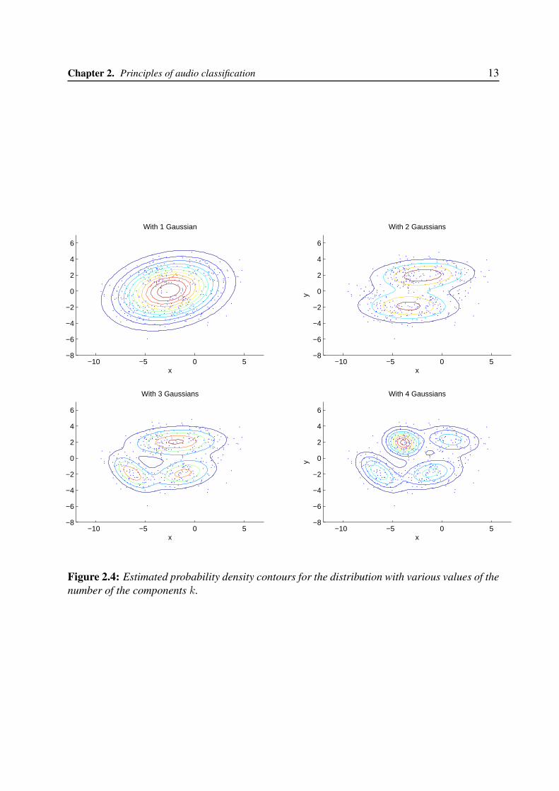
Fitting the data with a low number of Gaussians can lead to a bad fitting to the data. This isvisible looking at the resulting estimated probability density with various values of the numberof the components k in Figure 2.4.
2.2.3 Classification testOnce we trained the GMM, we can proceed to the classification test. This step consists in eval-uating the log-likelihood of a feature vector x in the model. Now we need a decision step todiscriminate if the features vector fits or not the model and say if the observation vector belongsto the model’s class3. This step will be explained in detail in Chapter 3.
3Note that we have to construct a GMM for each class we want to insert in our classifier. So if we have toclassify more than one class, we have to build a database in which all data/files must be divided into classes toseparate different data coming from different classes. It follows that each model will be trained over all the datareferred to a determinate class.
Chapter 2. Principles of audio classification 13
−10 −5 0 5−8
−6
−4
−2
0
2
4
6
x
With 1 Gaussian
−10 −5 0 5−8
−6
−4
−2
0
2
4
6
x
y
With 2 Gaussians
−10 −5 0 5−8
−6
−4
−2
0
2
4
6
x
With 3 Gaussians
−10 −5 0 5−8
−6
−4
−2
0
2
4
6
x
y
With 4 Gaussians
Figure 2.4: Estimated probability density contours for the distribution with various values of thenumber of the components k.

Chapter 3
Surveillance Algorithm for Recognition ofImpulsive Sounds (SARIS)
3.1 Sound Classification
3.1.1 Creation of the database of impulsive soundsIn order to create the models of the four classes of sounds (gunshots, screams, broken glasses andbarking dogs) we need a database of audio sounds. Unfortunately there are no Web database forthe classification of environmental sounds, while there are many for the speech/speaker recog-nition that, in addition to being large, are made with certain criteria designed for the testingpurpose. For example there are the Timit database1 and the Nist database2. So we have the prob-lem of creating an uniform database at home and the difficulty to deal with the literature becausethere is a common reference.
Our database has been created downloading audio files from “The Freesound Project”[19]without noise environment or eventually with a very high SNR. Every sound signal was storedwith some properties that are also the initial conditions and criteria for the well-functioning ofthe algorithm. Every sound signal:
• has a sampling rate of 44100 Hz and has only one channel (mono)3;
• has zero mean (the signal is centered on the x axis);
• is not normalized (the maximum absolute value of the signal is not necessarily 1);
• is cleaned from the first and last silence parts to create an homogeneous database and tohave a robust training step without frames of sounds that not concern about the “essence”of the sound class.
1http://www.ldc.upenn.edu/Catalog/CatalogEntry.jsp?catalogId=LDC93S1.2http://www.itl.nist.gov/iad/mig//tests/sre/.3Audio files with two channels (stereo) were transformed in one channel audio files (mono) summing the two
channels arrays and halving the values of the obtained array to avoid clipping (.wav files have a range that goes from-1 to 1).
15
16 GMM CLASSIFICATION OF ENVIRONMENTAL SOUNDS FOR SURVEILLANCE APPLICATIONS
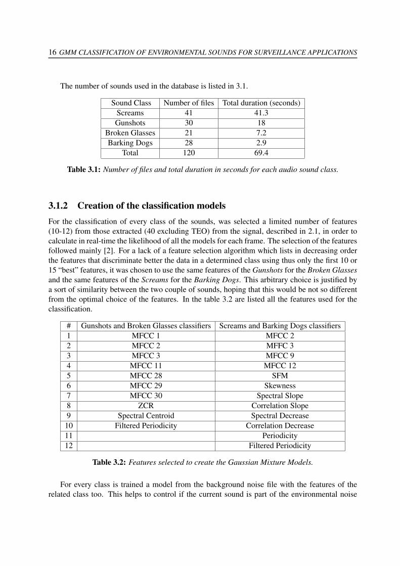
The number of sounds used in the database is listed in 3.1.
Sound Class Number of files Total duration (seconds)Screams 41 41.3Gunshots 30 18
Broken Glasses 21 7.2Barking Dogs 28 2.9
Total 120 69.4
Table 3.1: Number of files and total duration in seconds for each audio sound class.
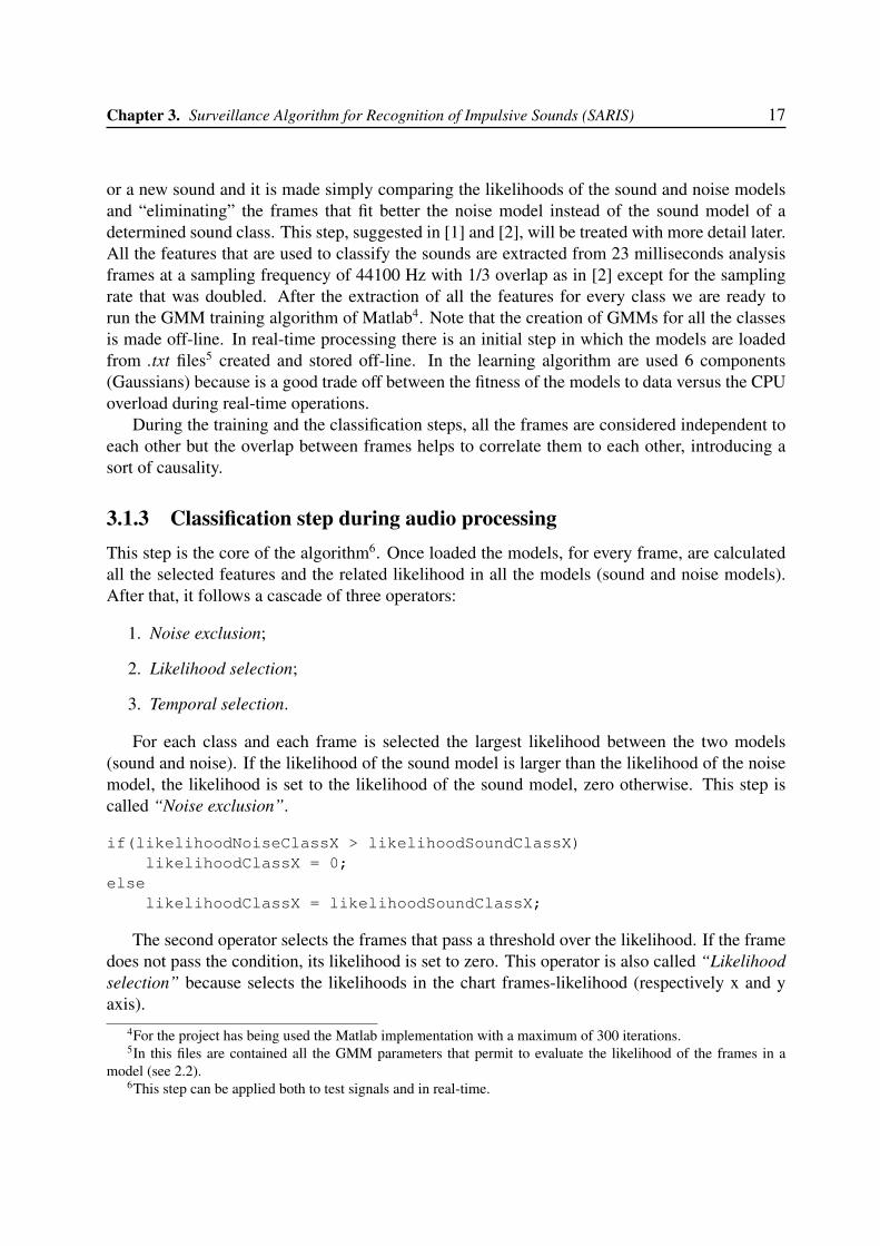
3.1.2 Creation of the classification modelsFor the classification of every class of the sounds, was selected a limited number of features(10-12) from those extracted (40 excluding TEO) from the signal, described in 2.1, in order tocalculate in real-time the likelihood of all the models for each frame. The selection of the featuresfollowed mainly [2]. For a lack of a feature selection algorithm which lists in decreasing orderthe features that discriminate better the data in a determined class using thus only the first 10 or15 “best” features, it was chosen to use the same features of the Gunshots for the Broken Glassesand the same features of the Screams for the Barking Dogs. This arbitrary choice is justified bya sort of similarity between the two couple of sounds, hoping that this would be not so differentfrom the optimal choice of the features. In the table 3.2 are listed all the features used for theclassification.
# Gunshots and Broken Glasses classifiers Screams and Barking Dogs classifiers1 MFCC 1 MFCC 22 MFCC 2 MFFC 33 MFCC 3 MFCC 94 MFCC 11 MFCC 125 MFCC 28 SFM6 MFCC 29 Skewness7 MFCC 30 Spectral Slope8 ZCR Correlation Slope9 Spectral Centroid Spectral Decrease
10 Filtered Periodicity Correlation Decrease11 Periodicity12 Filtered Periodicity
Table 3.2: Features selected to create the Gaussian Mixture Models.
For every class is trained a model from the background noise file with the features of therelated class too. This helps to control if the current sound is part of the environmental noise
Chapter 3. Surveillance Algorithm for Recognition of Impulsive Sounds (SARIS) 17
or a new sound and it is made simply comparing the likelihoods of the sound and noise modelsand “eliminating” the frames that fit better the noise model instead of the sound model of adetermined sound class. This step, suggested in [1] and [2], will be treated with more detail later.All the features that are used to classify the sounds are extracted from 23 milliseconds analysisframes at a sampling frequency of 44100 Hz with 1/3 overlap as in [2] except for the samplingrate that was doubled. After the extraction of all the features for every class we are ready torun the GMM training algorithm of Matlab4. Note that the creation of GMMs for all the classesis made off-line. In real-time processing there is an initial step in which the models are loadedfrom .txt files5 created and stored off-line. In the learning algorithm are used 6 components(Gaussians) because is a good trade off between the fitness of the models to data versus the CPUoverload during real-time operations.
During the training and the classification steps, all the frames are considered independent toeach other but the overlap between frames helps to correlate them to each other, introducing asort of causality.
3.1.3 Classification step during audio processingThis step is the core of the algorithm6. Once loaded the models, for every frame, are calculatedall the selected features and the related likelihood in all the models (sound and noise models).After that, it follows a cascade of three operators:
1. Noise exclusion;
2. Likelihood selection;
3. Temporal selection.
For each class and each frame is selected the largest likelihood between the two models(sound and noise). If the likelihood of the sound model is larger than the likelihood of the noisemodel, the likelihood is set to the likelihood of the sound model, zero otherwise. This step iscalled “Noise exclusion”.
if(likelihoodNoiseClassX > likelihoodSoundClassX)likelihoodClassX = 0;
elselikelihoodClassX = likelihoodSoundClassX;
The second operator selects the frames that pass a threshold over the likelihood. If the framedoes not pass the condition, its likelihood is set to zero. This operator is also called “Likelihoodselection” because selects the likelihoods in the chart frames-likelihood (respectively x and yaxis).
4For the project has being used the Matlab implementation with a maximum of 300 iterations.5In this files are contained all the GMM parameters that permit to evaluate the likelihood of the frames in a
model (see 2.2).6This step can be applied both to test signals and in real-time.
18 GMM CLASSIFICATION OF ENVIRONMENTAL SOUNDS FOR SURVEILLANCE APPLICATIONS
if(likelihoodClassX < likelihoodThresholdClassX)likelihoodClassX = 0;
Now that the candidate frames are selected, is applied the third operator that is divided in twosteps:
• Weighted Moving Average (WMA) of the likelihoods with a fixed number of frames for thewindow called numFramesWMA;
• selection of the likelihoods using a number of frames as threshold numFramesWMADurationlarger than numFramesWMA.
For the fist step was implemented a WMA defined as:
WMAM =n · pM + (n− 1) · p(M−1) + · · ·+ 2 · p(M−n+2) + p(M−n+1)
n+ (n− 1)− · · ·+ 2 + 1(3.1)
were p is the array of values and M = numFramesWMA is the window length.When calculating the WMA across successive values, it can be noted that the difference
between the numerators of WMAM+1 and WMAM is n · pM+1 − pM − · · · − pM−n+1. If wedenote the sum pM + ...+ pM−n+1 by TotalM , then
TotalM+1 = TotalM + pM+1 − pM−n+1 (3.2)
NumeratorM+1 = NumeratorM + n · pM+1 − TotalM (3.3)
WMAM+1 =NumeratorM+1
n+ (n− 1) + · · ·+ 2 + 1(3.4)
In the second step, are discarded all the frames that have a number of consecutive positivevalues of the WMA less to numFramesWMADuration. In other words is used a binaryvariable associated to every frame of every sound class that determines if there was or not asound of a determined class.
if(PassTemporalDuration)FrameEventClassX = 1;
elseFrameEventClassX = 0;
This passage is made to avoid that sporadic and isolated frames that pass the Noise exclusionand the Likelihood selection steps detecting an event only for a single frame duration. In factWMA flats the “spiky” values and permits to have an homogeneous likelihood. This operatoris called “Temporal selection” because it considers only the frames that overcome the thresholdfor a determinate number of frames which can be seen as a temporal constraint. The thresholds
Chapter 3. Surveillance Algorithm for Recognition of Impulsive Sounds (SARIS) 19
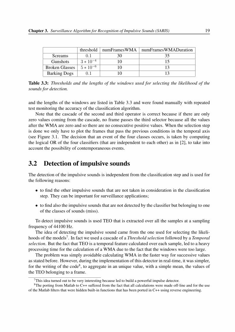
threshold numFramesWMA numFramesWMADurationScreams 0.1 30 35Gunshots 3 ∗ 10−4 10 15
Broken Glasses 5 ∗ 10−6 10 13Barking Dogs 0.1 10 13
Table 3.3: Thresholds and the lengths of the windows used for selecting the likelihood of thesounds for detection.
and the lengths of the windows are listed in Table 3.3 and were found manually with repeatedtest monitoring the accuracy of the classification algorithm.
Note that the cascade of the second and third operator is correct because if there are onlyzero values coming from the cascade, no frame passes the third selector because all the valuesafter the WMA are zero and so there are no consecutive positive values. When the selection stepis done we only have to plot the frames that pass the previous conditions in the temporal axis(see Figure 3.1. The decision that an event of the four classes occurs, is taken by computingthe logical OR of the four classifiers (that are independent to each other) as in [2], to take intoaccount the possibility of contemporaneous events.
3.2 Detection of impulsive soundsThe detection of the impulsive sounds is independent from the classification step and is used forthe following reasons:
• to find the other impulsive sounds that are not taken in consideration in the classificationstep. They can be important for surveillance applications;
• to find also the impulsive sounds that are not detected by the classifier but belonging to oneof the classes of sounds (miss).
To detect impulsive sounds is used TEO that is extracted over all the samples at a samplingfrequency of 44100 Hz.
The idea of detecting the impulsive sound came from the one used for selecting the likeli-hoods of the models7. In fact we used a cascade of a Threshold selection followed by a Temporalselection. But the fact that TEO is a temporal feature calculated over each sample, led to a heavyprocessing time for the calculation of a WMA due to the fact that the windows were too large.
The problem was simply avoidable calculating WMA in the faster way for successive valuesas stated before. However, during the implementation of this detector in real-time, it was simpler,for the writing of the code8, to aggregate in an unique value, with a simple mean, the values ofthe TEO belonging to a frame.
7This idea turned out to be very interesting because led to build a powerful impulse detector.8The porting from Matlab to C++ suffered from the fact that all calculations were made off-line and for the use
of the Matlab filters that were hidden built-in functions that has been ported in C++ using reverse engineering.

20 GMM CLASSIFICATION OF ENVIRONMENTAL SOUNDS FOR SURVEILLANCE APPLICATIONS
Therefore, 23 milliseconds windows were used to calculate the TEO feature with 1/3 overlapas in the classifier. In a second time, when the two detectors were divided in two NMM nodes,were avoided overlapping windows and the TEO’s mean was calculated only over a windowframe with length equal to the window step (about 7.6 milliseconds). In other words, now, isextracted only one TEO value per frame without overlap; it can be considered actually a soundfeature like the others used to classify the sound. The parameters used in the operators are listedin Table 3.3.
threshold numFramesWMA numFramesWMADuration5 ∗ 10−5 5 7
Table 3.4: Threshold and the length of the windows used for selecting the TEO-signal of thesound.
Summarizing, it follows that the system achieves the detection of an impulsive sound withonly one feature!
3.3 Audio test creationTesting was made using two types of audio test signals:
1. test signals for the accuracy calculation;
2. test signals for real-time testing.
In the first type the duration of the test is equal to the duration of the database tests. The newfile is created by selecting a random piece of the background noise signal and adding a randomsignal of the database. The length of the noise audio signal is the equal to that of the pure audiosignal. The addition is weighted by the 0 ≤ NoiseAmplitudeModulation ≤ 1. To avoidclipping in .wav files is used this formula:
newSound = NoiseAmplitudeModulation · cut+ (1−NoiseAmplitudeModulation) · pureSound (3.5)
where cut is the piece of the background noise signal and pureSound is the clean signal fromthe database.
The Signal-To-Noise Ratio (SNR) of a new audio file with noise for the accuracy calculationis:
SNR{dB} = 10 · log10(Se/Ne) (3.6)
where Se is the total energy of the clean signal∑
n(pureSound[n]2) and Ne is the total
energy of the noise signal∑
n(cut[n]2). Note that this formula is correct because the two signals
pureSound and cut have exactly the same length.

Chapter 3. Surveillance Algorithm for Recognition of Impulsive Sounds (SARIS) 21
In the second type, tests are 20 seconds long (duration of the background noise used9): inthis time lag is inserted in a random position10, an arbitrary number of sounds taken from thedatabase (as in Figure 3.1).
Figure 3.1: Visualization of likelihood and detection in time. The upper plot is the detection overthe time and in the other plots there are the values of the likelihood of each model. Legend: black- impulsive sound; red - gunshots; green - screams; blue - broken glasses; light blue - barkingdogs.
9Extract from an audio file taken in a London square downloaded from [19].10Overlap between sounds can occur so it is possible to see the independence of each classifier in relation to the
others

Chapter 4
Development tools and Network-IntegratedMultimedia Middleware (NMM)
4.1 Development tools
In this section are listed all the development tools used in the project.
4.1.1 Middleware
• Network-Integrated Multimedia Middleware (NMM) described in deep detail in this chap-ter.
4.1.2 Software tools
4.1.2.1 Programming languages
The programming languages used for the implementation of the software are:
• Matlab - Octave;
• C/C++.
4.1.2.2 Integrated Development Environment (IDE)
The Integrated Development Environment (IDE) used are:
• Microsoft Visual Studio 2008 (for C++ Windows implementation);
• Eclipse (for C++ Linux implementation).
23
24 GMM CLASSIFICATION OF ENVIRONMENTAL SOUNDS FOR SURVEILLANCE APPLICATIONS
4.1.2.3 Operative Systems (OS)
The OS used are:
• Windows (XP - 7);
• Ubuntu 9.04 - 9.10.
4.1.2.4 Graphic User Interface (GUI)
For plotting charts of both off-line and real-time tests, it was used the Freeware library ChartDi-rector [20].
4.1.2.5 Subversion (SVN)
Subversion (also known as SVN) is an open source version control system designed by CollabNetInc used for:
• saving and updating the source files of the project;
• comparing different chronological versions of the project for consideration of possibleerrors due to changes and updates;
• merging different versions of the same source file.
This tool was so helpful because the files were always protected from data loss and it fastenedthe update from one computer to another, also with different SO.
4.1.3 Audio toolsThese tools are used mainly for the real-time tests:
• external sound card: Edirol UA-101: USB Audio Interface by Roland1;
• microphone: SM58 by Shure2;
• loud speaker: MP2-A Compact Amplified Monitor System by Generalmusic.
For the creation of the database of sounds is used the following software:
• Audacity. Sound editor for cutting audio files3;
• Matlab - Octave. Functions for reading the .wav files.1http://www.rolandus.com/products/productdetails.php?ProductId=703.2http://www.shure.com/americas/products/microphones/sm/
sm58-vocal-microphone3http://audacity.sourceforge.net/.
Chapter 4. Development tools and Network-Integrated Multimedia Middleware (NMM) 25
4.2 Introduction to NMM
This section is a description of NMM taken from the NMM documentation [21]. Besides the PC,an increasing number of multimedia devices - such as set-top boxes, PDAs, and mobile phones- already provide networking capabilities. However, today’s multimedia infrastructures adopt acentralized approach, where all multimedia processing takes place within a single system. Thenetwork is, at best, used for streaming predefined content from a server to clients. Conceptually,such approaches consist of two isolated applications, a server and a client (see Figure 4.1). Therealization of complex scenarios is therefore complicated and error-prone, especially since theclient has typically no or only limited control of the server.
Figure 4.1: Client/server streaming consists of two isolated applications that do not providefine-grained control or extensibility.
The Network-Integrated Multimedia Middleware (NMM) [21] overcomes these limitationsby enabling access to all resources within the network: distributed multimedia devices and soft-ware components can be transparently controlled and integrated into an application. In contrastto all other multimedia architectures available, NMM is a middleware, i.e. a distributed softwarelayer running in between distributed systems and application (see Figure 4.2).
Figure 4.2: A multimedia middleware is a distributed software layer that eases applicationdevelopment by providing transparency.
26 GMM CLASSIFICATION OF ENVIRONMENTAL SOUNDS FOR SURVEILLANCE APPLICATIONS
As an example, this allows the quick and easy development of an application that receivesTV from a remote device – including the transparent control of the distributed TV receiver.Even a PDA with only limited computational power can run such an application: the mediaconversions needed to adapt the audio and video content to the resources provided by the PDAcan be distributed within the network. While the distribution is transparent for developers, nooverhead is added to all locally operating parts of the application. To this end, NMM also aimsat providing a standard multimedia framework for all kinds of desktop applications.
NMM is both an active research project at Saarland University in Germany and an emergingOpen Source project. NMM runs on a variety of operating systems and hardware platforms.NMM is implemented in C++, and distributed under a dual-license: NMM is released under“free” licenses, such as the GPL, and commercial licenses.
4.2.1 Nodes, Jacks, and Flow Graphs
The general design approach of the NMM architecture is similar to other multimedia architec-tures. Within NMM, all hardware devices (e.g. a TV board) and software components (e.g.decoders) are represented by so called nodes. A node has properties that include its input andoutput ports, called jacks, together with their supported multimedia formats. A format preciselydefines the multimedia stream provided, e.g. by specifying a human readable type, such as “au-dio/raw” for uncompressed audio streams, plus additional parameters, such as the sampling rateof an audio stream. Since a node can provide several inputs or outputs, its jacks are labelled withtags. Depending on the specific kind of a node, its innermost loop produces data, performs acertain operation on the data, or consumes data.
The system distinguishes between different types of nodes: a source produces data and hasone output jack. A sink consumes data, which it receives from its input jack. A filter has oneinput and one output jack. It only modifies the data of the stream and does not change its formator format specific parameters. A converter also has one input and one output jack but can changethe format of the data (e.g. from raw video to compressed video) or may change format specificparameters (e.g. the video resolution). A multiplexer has several input jacks and one output jack;a demultiplexer has one input jack and several output jacks. Furthermore, there is also a genericmux-demux node available. In section 4.4 will be explained step-by-step how to develop a newnode.
These nodes can be connected each other to create a flow graph, where every two connectedjacks need to support a “matching” format, i.e. the formats of the connected input jack respec-tively output jack need to provide the same type and all parameters and the respective valuespresent in one format need to be available for the other and vice versa. The structure of thisgraph then specifies the operation to be performed, e.g. the decoding and playback of an MP3file (see Figure 4.3).
Together, more than 60 nodes are already available for NMM, which allows for integratingvarious input and output devices, codecs, or specific filters into an application.
Chapter 4. Development tools and Network-Integrated Multimedia Middleware (NMM) 27
Figure 4.3: A flow graph for playing back MP3 files.
4.2.2 Messaging System
The NMM architecture uses a uniform messaging system for all communication. There are twotypes of messages. Multimedia data is placed into buffers. Event forward control informationsuch as a change of speaker volume. Events are identified by a name and can include arbitrarytyped parameters.
There are two different types of interaction paradigms used within NMM. First, messagesare streamed along connected jacks. This type of interaction is called instream and is most oftenperformed in downstream direction, i.e. from sources to sinks; but NMM also allows for sendingmessages in upstream direction.
Notice that both buffers and events can be sent instream. For instream communication, socalled composite events are used that internally contain a number of events to be handled withina single step of execution. Instream events are very important for multimedia flow graphs. Forexample, the end of a stream (e.g. the end of a file) can be signalled by inserting a specific eventat the end of a stream of buffers. External listener objects can be registered to be notified whencertain events occur at a node (e.g. for updating the GUI upon the end of a file or for selecting anew file).
Events are also employed for the second type of interaction called out-of-band, i.e. interactionbetween the application and NMM objects, such as nodes or jacks. Events are used to controlobjects or for sending notifications from objects to registered listeners.
4.2.3 Interfaces
In addition to manually sending events, object-oriented interfaces allow to control objects bysimply invoking methods, which is more type-safe and convenient then sending events. Theseinterfaces are described in NMM Interface Definition Language (NMM IDL) that is similar toCORBA IDL. According to the coding style of NMM, interfaces start with a capital “I”. Foreach description, an IDL compiler creates an interface and a implementation class. While animplementation class is used for implementing specific functionality within a node, an interfaceclass is exported for interacting with objects. During runtime, supported events and interfacescan be queried by the application. Notice that interfaces described in NMM IDL describe out-of-band and instream interaction.
28 GMM CLASSIFICATION OF ENVIRONMENTAL SOUNDS FOR SURVEILLANCE APPLICATIONS
4.2.4 Distributed Flow Graphs
What is special about NMM is the fact that NMM flow graphs can be distributed across thenetwork: local and remote multimedia devices or software components encapsulated withinnodes can be controlled and integrated into a common multimedia processing flow graph, a dis-tributed flow graph. While this distribution is transparent for application developers, no overheadis added to all locally operating parts of the graph: In such cases, references to already allocatedmessages are simply forwarded - no networking is performed at all.
The following shows an example for a distributed flow graph for playing back encoded (com-pressed) files, e.g. MP3 files. A source node for reading data from the local file system (Au-dioReader) is connected to a node for decoding audio streams (AudioDecoder). This decoderis connected to a sink node for rendering uncompressed audio using a sound board (AudioRen-derer). Once the graph is started, the source nodes reads a certain amount of data from a givenfile, encapsulates it into buffers, e.g. of size 1024 bytes, and forwards these buffers to its succes-sor. After being decoded to uncompressed “raw” audio, the converter node forwards data buffersto the sink node (see Figure 4.4).
Figure 4.4: A distributed flow graph for playing back MP3 files.
The application controls all parts of this flow graph using interfaces, e.g. INode for control-ling the generic aspects of all instantiated nodes. Notice that three different hosts are present inour example. The application itself runs on host1, the source node on host2, and the decoder andsink node on host3. Therefore, NMM automatically creates networking connections betweenthe application and the three distributed nodes (out-of-band interaction), but also between thesource and the decoder node (instream interaction). Therefore, compressed MPEG audio data istransmitted over the network.
Notice that such a simple but distributed flow graph already provides many benefits. First,it allows an application to access files stored on distributed systems without the need for a dis-tributed file system, such as NFS. Second, the data streaming between connected distributednodes is handled automatically by NMM. Third, the application acts as “remote control” for all

Chapter 4. Development tools and Network-Integrated Multimedia Middleware (NMM) 29
distributed nodes. As an example, this allows for transparently changing the output volume of theremote sound board by a simple method invocation on a specific interface, e.g. IAudioDevice.
4.2.5 Distributed Synchronization
Since NMM flow graphs can be distributed, they allow for rendering audio and video on differentsystems. For example, the video stream of an MPEG2 file can be presented on a large screenconnected to a PC while the corresponding audio is played on a mobile device. To realize syn-chronous playback of nodes distributed across the network, NMM provides a generic distributedsynchronization architecture. This allows for achieving lip-synchronous playback as requiredfor the above described setup. In addition, media presentations can also be performed on severalsystems simultaneously. A common application is the playback of the same audio stream usingdifferent systems located in different rooms of a household - a home-wide music system.
The basis for performing distributed synchronization is a common source for timing informa-tion. It is used a static clock within each address space. This clock represents the system clockthat is globally synchronized by the Network Time Protocol (NTP) and can therefore be assumedto represent the same time basis throughout the network. With the current setup, it is found thetime offset between different systems to be in the range of 1 to 5 ms, which is sufficient for thepurpose of the current thesis project.
4.2.6 Registry Service
The registry service in NMM allows discovery, reservation, and instantiation of nodes availableon local and remote hosts. On each host a unique registry server administrates all NMM nodesavailable on this particular system. For each node, the server registry stores a complete nodedescription that includes the specific type of a node (e.g. “sink”), its name (e.g. “Playbac-kNode”), the provided interfaces (e.g. “IAudioDevice” for increasing or decreasing the outputvolume), and the supported input and output formats (e.g. an input format “audio/raw” includingadditional parameters, such as the sampling rate).
The application uses a registry client to send requests to registry servers running on either thelocal or remote hosts. Registry servers are contacted by connecting to a well-known port. Aftersuccessfully processing the request the server registry reserves the requested nodes. Nodes arethen created by a factory either on the local or remote host. For nodes to be instantiated on thesame host, the client registry will allocate objects within the address space of the application toavoid the overhead of an interprocess communication.
To setup and create complex distributed flow graphs, an application can either request eachnode separately or use a graph description as query. Such a description includes a set of nodedescriptions connected by edges.
For an application to be able to create a distributed flow graph, the NMM application calledserverregistry needs to be running on each participating host. For purely locally operating appli-cations this is not required. Then, a server registry is running within the application itself but notaccessible from remote hosts.
30 GMM CLASSIFICATION OF ENVIRONMENTAL SOUNDS FOR SURVEILLANCE APPLICATIONS
Before a server registry can be used, it needs to determine which devices and software com-ponents are available on a particular host. Therefore, the registry needs to be initialized onceusing following command:
user@linux:˜/nmm/bin> ./serverregistry -s
Create config file with plugin information ...Loading plugins...AC3DecodeNode availableAVDemuxNode availableAVIReadNode available... and many further nodes
Config file successfully written.
4.2.7 Clic - An Application for Setting up NMM Multimedia Flow GraphsThe NMM framework is used to build up multimedia applications. The basic components in thisframework are nodes which perform a certain functionality, like reading a video file or decodingit. Such nodes can be connected to a flow graph to perform a certain task like watching a film ortranscoding it into another format.
Especially transcoder jobs do not need any additional user interaction if the application isrunning. Writing such an application without any user interaction is currently straightforward.First, the application requests these nodes from the registry, connects them to a flow graph andfinally starts the entire flow graph.
To use the features provided by NMM we can follow two procedures. The first and easiestis discussed in this section and is based on the use of the executable clic; the second is to write,compile and run C++ code that uses libraries, namespaces and interfaces of NMM as can be seenin the helloworld examples located in the folder examples of NMM.
The application clic is used to build such a standard NMM application automatically from atextual description. clic stands for Command Line Interaction and Configuration and providesa tool for using the existing nodes with the possibility to configure some of their parameters.Starting from the knowledge of the functions of each node, textitclic can create a flow graphfrom its textual description which is called “graph description”. With clic becomes very easy towrite and run an application that does not require interaction with a user; just correctly create afile with extension .gd (graph description) and run it with clic.
Will now follow the details of the syntax of the graph description and the usage of the clicapplication.
A graph description consists of two major parts. The first part is an (optional) commentintroduced by the character %. The second part specifies the flow graph which describes how toconnect the nodes. The following example describes a simple graph to play a .wav audio file.
% This graph description realizes a simple WAV player.% Use the -i option of clic to specify an WAV file
Chapter 4. Development tools and Network-Integrated Multimedia Middleware (NMM) 31
WavReadNode ! ALSAPlaybackNode
To run this graph description, copy it into a file, e.g. wavplay.gd, and start clic with thefollowing command:
./clic wavplay.gd -i /home/username/audio/song.wav
The option “-i” is used to specify the input file. To exit the application, enter “q” at thecommand line and press enter.
The flow graph section of a graph description describes how to connect the nodes. A nodeis identified by its name, which is (normally) the C++ class name. The exclamation mark (!) isused to denote a connection between two nodes as seen in the graph description for playing WAVfiles. In this example the statement:
WavReadNode ! ALSAPlaybackNode
results in clic to request the nodes WavReadNode and ALSAPlaybackNode. If all nodes canbe successfully requested, the WavReadNode is connected to the ALSAPlaybackNode. Then,clic sets the specified parameters from the command line, for example an input file, and starts theentire flow graph.
In several cases a node must be configured before it can be used. In the previous examples,the name of a .wav file needs to be specified for the WavReadNode to read data from this file.Even though the clic-application offers a command line arguments for such a scenario, othernodes might require additional parameters, which can not be specified in this way. In this case,you ust call a node’s specific method, offered by an NMM interface specified in NMM-IDL(Interface Definition Language). Each method of an NMM interface can be called from graphdescription as well. For this purpose you have to write the corresponding IDL method with allarguments prefaced by the character “$”. Furthermore you have to specify the state in whichthe method must be executed. For example the WavReadNode offers the method setFilenamein one of its interfaces to set a WAV file, which must be called in the state INITIALIZED. Fur-thermore you might want to change the queue of the ALSAPlaybackNode for incoming buffers,which can be done using the method setDownstreamMaxSize which must be called in the stateCONSTRUCTED. The following example shows how to call these two methods from a graphdescription.
% This graph description describes a simple WAV player and shows% how to call interface methods from a graph description. It is% not required to set the input file using the option -i of clic.WavReadNode $ setFilename("/home/username/audio/song.wav")INITIALIZED
! ALSAPlaybackNode $ setDownstreamMaxSize(1, "default") CONSTRUCTED
32 GMM CLASSIFICATION OF ENVIRONMENTAL SOUNDS FOR SURVEILLANCE APPLICATIONS
As can be seen in this example, the methods to be called are specified with their commonname and additional parameters followed by the state of the node in which they should be exe-cuted.
Be careful using this feature. The given arguments are read as strings and converted to theexpected type. Thus, it can cause errors if you set invalid arguments. Furthermore, you mustspecify all arguments: default arguments are currently not supported.
4.3 Installation of NMM
The middleware was installed using the 9.04 and 9.10 Ubuntu releases. It is also available towork in virtual machines because the emulation of the hardware peripherals like the sound cardor video card does not create problems for the manage of the middleware.
4.3.1 Hardware prerequisites
For the Linux installation is needed a rightly configured video card with the Xv (X-Video) ex-tension. This extension indicates a mechanism of output video for the X-Window system whichis a windows visualization protocol used mainly in Unix-like systems. To know if it is all rightrun the following command:
xvinfo
This command prints all the informations of the video card for the X-Video extension. Ifit prints the settings of the video card then no changes are necessary, otherwise it returns anerror. In this case you have to verify the correct installation of the xvinfo package on the Linuxdistribution used.
NMM also need a sound card or an audio chip able to reproduce sounds at different samplingrates (e.g. at 44.1 KHz). At present each personal computer has a sound card with this function-ality integrated. By the way the precondition implies the proper recognition of the hardware bythe operating system.
4.3.2 Network configuration
To configure the network must be opened all ports 22801 and the interval 5000-6000, that’s tosay that they should not be blocked by firewalls or other protection systems. Then it is necessaryto set the hosts’ file which are usually located in the /etc/hosts folder. Here we have to enter thedomain, the hostname, and then, if there is a DNS (Domain Name System), we must also enterthe IP addresses because NMM is unable to recognize them directly.
Chapter 4. Development tools and Network-Integrated Multimedia Middleware (NMM) 33
4.3.3 Software configuration
Before installing NMM we have to prepare the working environment. Specifically, working withUbuntu, many of the packages required for the proper functioning of the middleware were absentand therefore it was required a prior installation. There are three ways to install:
• download the archive available by Motama containing the precompiled libraries and un-pack it in a folder. These libraries do not necessarily cover all requirements and also doesnot guarantee the correctness of the operations in all system. The method is simple, butcan sometimes cause problems redirecting thus to one of the following two options;
• download, compile and install the libraries using the source codes. All the informationsand descriptions of the libraries needed for the right functioning are listed in A;
• install the package on the Linux distribution used. Beware that many distributions providethe header files, divided by library files called developer4.
It is recommended to use the first solution, which involves a simple download of a packageof already precompiled libraries (e.g. nmm-2.2.0-optional-external-libs-linux.tar.gz) and installit by following these instructions:
cd /home/username/tar xvfz nmm-2.2.0-optional-external-libs-linux.tar.gz
Despite the advice, this alternative did not achieve the desired results, because after the in-stallation of NMM many nodes were still not available. The second alternative, instead, wassuccessful.
There are libraries for the management of audio such as “asoundlib”, for the manage ofthe video as “Xlib” and for the interaction with various devices. Of course, for a completeinstallation, all the libraries should be installed; but if, for example, the firewire cameras are notused, the libraries “l1394” may be omitted.
Once identified the libraries, the installation can be done simply by using the Synaptic Pack-age Manager in Ubuntu, making sure to install from the list all the files *-dev. Some libraries,however, are not available through Synaptic and then require manual installation (for example,the ALSA libraries for managing audio).
Once prepared the environment, you can proceed with the actual installation of NMM. Fromsite Motama you need to download the latest release (e.g. the file nmm-2.2.0.tar.gz) and unzip itto a folder (e.g. /home/username/nmm). From this new folder give these commands in sequence:
./configuremakesudo make install
4If a package is called libABC, the package developer file will call most likely libABC-developer or libABC-dev.

34 GMM CLASSIFICATION OF ENVIRONMENTAL SOUNDS FOR SURVEILLANCE APPLICATIONS
The ./configure permits to see which basic functions of NMM are enabled. At the beginningthere should be entries marked disabled, but after the installation of all external packages, theitems concerned should all be marked enabled. After performing these steps, if no errors occurs,NMM should be properly installed.
As a first test you can try the command:
serverregistry -s
that returns the list of all available nodes. The following is an example of the result of thiscommand:
serverregistry and Network-IntegratedMultimedia Middleware (NMM) Version 2.2.0
Copyright (C) 2005-2010Motama GmbH, Saarbruecken, Germanyhttp://www.motama.com
See licence for terms and conditions of usage
No plugin information available! If you start NMM forthe first time this information is created automatically.Note: If you ever change your hardware configuration orupdate the NMM version you must delete the file/home/username/.nmm/plugins.2.2.0.xps._usr_localor run ’serverregistry -s’ again.
Create config file with plugin information ...Loading plugins...AC3DecodeNode availableAC3ParseNode availableALSAPlaybackNode availableALSARecordNode availableAVDemuxNode availableAVMuxNode availableAnalyseDataIdNode availableAudioMuxNode availableBrightnessNode availableBufferDropNode availableBufferShapingNode availableBufferTimestampControlNode availableBufferTimestampNode availableCopyNode availableDVBS2ReadNode not availableDVBSimulatorNode availableDevNullNode available
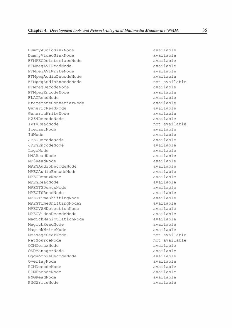
Chapter 4. Development tools and Network-Integrated Multimedia Middleware (NMM) 35
DummyAudioSinkNode availableDummyVideoSinkNode availableFFMPEGDeinterlaceNode availableFFMpegAVIReadNode availableFFMpegAVIWriteNode availableFFMpegAudioDecodeNode availableFFMpegAudioEncodeNode not availableFFMpegDecodeNode availableFFMpegEncodeNode availableFLACReadNode availableFramerateConverterNode availableGenericReadNode availableGenericWriteNode availableH264DecodeNode availableIVTVReadNode not availableIcecastNode availableIdNode availableJPEGDecodeNode availableJPEGEncodeNode availableLogoNode availableM4AReadNode availableMP3ReadNode availableMPEGAudioDecodeNode availableMPEGAudioEncodeNode availableMPEGDemuxNode availableMPEGReadNode availableMPEGTSDemuxNode availableMPEGTSReadNode availableMPEGTimeShiftingNode availableMPEGTimeShiftingNode2 availableMPEGVSHDetectionNode availableMPEGVideoDecodeNode availableMagickManipulationNode availableMagickReadNode availableMagickWriteNode availableMessageSeekNode not availableNetSourceNode not availableOGMDemuxNode availableOSDManagerNode availableOggVorbisDecodeNode availableOverlayNode availablePCMDecodeNode availablePCMEncodeNode availablePNGReadNode availablePNGWriteNode available
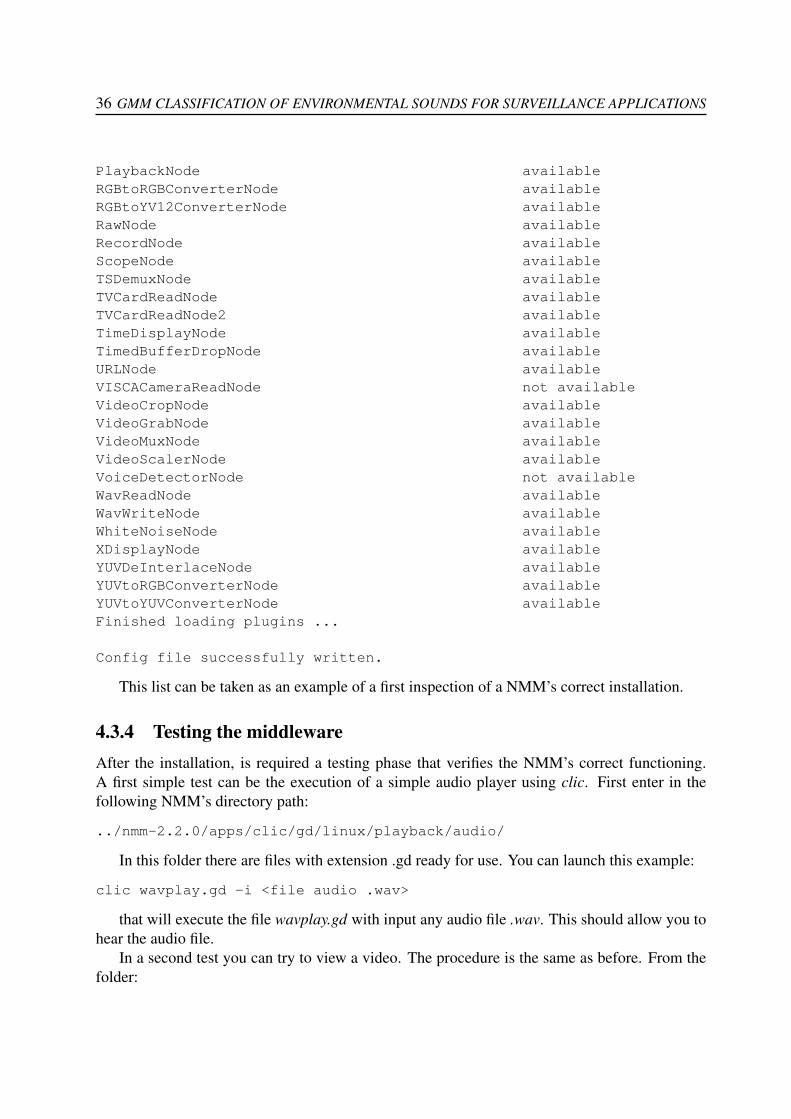
36 GMM CLASSIFICATION OF ENVIRONMENTAL SOUNDS FOR SURVEILLANCE APPLICATIONS
PlaybackNode availableRGBtoRGBConverterNode availableRGBtoYV12ConverterNode availableRawNode availableRecordNode availableScopeNode availableTSDemuxNode availableTVCardReadNode availableTVCardReadNode2 availableTimeDisplayNode availableTimedBufferDropNode availableURLNode availableVISCACameraReadNode not availableVideoCropNode availableVideoGrabNode availableVideoMuxNode availableVideoScalerNode availableVoiceDetectorNode not availableWavReadNode availableWavWriteNode availableWhiteNoiseNode availableXDisplayNode availableYUVDeInterlaceNode availableYUVtoRGBConverterNode availableYUVtoYUVConverterNode availableFinished loading plugins ...
Config file successfully written.
This list can be taken as an example of a first inspection of a NMM’s correct installation.
4.3.4 Testing the middlewareAfter the installation, is required a testing phase that verifies the NMM’s correct functioning.A first simple test can be the execution of a simple audio player using clic. First enter in thefollowing NMM’s directory path:
../nmm-2.2.0/apps/clic/gd/linux/playback/audio/
In this folder there are files with extension .gd ready for use. You can launch this example:
clic wavplay.gd -i <file audio .wav>
that will execute the file wavplay.gd with input any audio file .wav. This should allow you tohear the audio file.
In a second test you can try to view a video. The procedure is the same as before. From thefolder:
Chapter 4. Development tools and Network-Integrated Multimedia Middleware (NMM) 37
nmm-2.2.0/apps/clic/gd/linux/playback/video/
give:
clic noise.gd
which should show a display window with video noise.
4.4 Software Developer Kit (SDK)Motama provides a kit called NMM-SDK for software’s development. Actually, this kit consistsof a simple interface in NMM-IDL, a plugin that implements this interface and a flow graph usingthese two components, namely providing an example of what a developer should do to create hisown plugins recognizable from the registry service (usable in a flow graph) and how to use them.
Let’s see how to install the NMM-SDK. The most important prerequisite is the correct in-stallation of NMM. After NMM’s installation, download the SDK-package from the web (e.g.nmm-sdk-2.2.0) and unpack it. Now from the SDK folder give:
./configure --with-nmm=/usr/localmakesudo make install
After the installation, go inside the folder:
...nmm-sdk-2.2.0/nmm/plugins/audio/filter
in which there is an example node, AudioVolumeFilterNode, that can open a file .wav andadjust the volume from the shell. The recommended way to learn how to build new nodes is tocreate an own node or otherwise modify the AudioVolumeFilterNode to take inspiration from it.
Watching .cpp files it is easy to understand the NMM’s syntax but the first problem is tryingto build the project including other external files (.cpp and .hpp) with the file AudioVolume-Filter.cpp.
To do this we must include in make.am the files used:
libnmmMyNode_la_SOURCES = \MyNode.cpp \file1.cpp \file2.cpp
treepkginclude_HEADERS = \$(IDLHEADERS) \MyNode.hpp \file1.hpp \file2.hpp
38 GMM CLASSIFICATION OF ENVIRONMENTAL SOUNDS FOR SURVEILLANCE APPLICATIONS
After editing the make.am file from the SDK directory we need to use the autotools functions5
to generate the make.in and subsequently the makefile:
chmod +x autogen.sh && ./autogen.sh
Now we have everything ready. Now just give a reconfiguration, remembering that the SDKrequires the NMM installation path:
./configure --with-nmm=/usr/local
Now that we generated the makefiles, we have to write from the SDK root:
makesudo make install
If all ends without errors, writing:
serverregistry -s
you should see the name of our new node in the list:
MyNode available
Note that if you use external libraries in your code, they have to be added into make.am.
4.5 Audio Surveillance GraphThe Audio Surveillance Graph is a cascade of five nodes, simply described by the clic syntax:
RecordNode $setDevice("/dev/audio1") CONSTRUCTED!ImpulseDetectorNode!AudioClassificationNode!AudioEventReceiverNode!XDisplayNode
The RecordNode, a SourceNode, records the sound at a fixed framerate and bitrate (respec-tively 44100 Hz and 16 bit/value) and sends the signal to the ImpulseDetectorNode that is aFilterNode like AudioClassificationNode. FilterNodes are nodes that have the output signal thatis the same of the input signal and they only make an analysis and processing step of the signal.When they found an event, they notify it with an event-message that is propagated downstream inthe graph. The AudioEventReceiverNode, a GenericFilterNode, is a listener of the graph eventsand catch all the events launched by the ImpulseDetectorNode and the AudioClassificationNode.GenericFilterNodes are nodes that have an input format different from the output one. In fact the
5For those not familiar with autotools or those who want to know more, take a look at this on-line guide http://sourceware.org/autobook/autobook/autobook_toc.html.
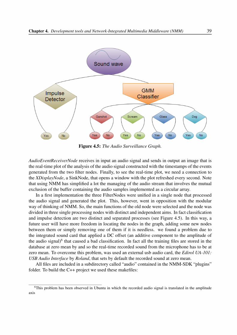
Chapter 4. Development tools and Network-Integrated Multimedia Middleware (NMM) 39
Figure 4.5: The Audio Surveillance Graph.
AudioEventReceiverNode receives in input an audio signal and sends in output an image that isthe real-time plot of the analysis of the audio signal constructed with the timestamps of the eventsgenerated from the two filter nodes. Finally, to see the real-time plot, we need a connection tothe XDisplayNode, a SinkNode, that opens a window with the plot refreshed every second. Notethat using NMM has simplified a lot the managing of the audio stream that involves the mutualexclusion of the buffer containing the audio samples implemented as a circular array.
In a first implementation the three FilterNodes were unified in a single node that processedthe audio signal and generated the plot. This, however, went in opposition with the modularway of thinking of NMM. So, the main functions of the old node were selected and the node wasdivided in three single processing nodes with distinct and independent aims. In fact classificationand impulse detection are two distinct and separated processes (see Figure 4.5). In this way, afuture user will have more freedom in locating the nodes in the graph, adding some new nodesbetween them or simply removing one of them if it is needless. we found a problem due tothe integrated sound card that applied a DC offset (an additive component to the amplitude ofthe audio signal)6 that caused a bad classification. In fact all the training files are stored in thedatabase at zero mean by and so the real-time recorded sound from the microphone has to be atzero mean. To overcome this problem, was used an external usb audio card, the Edirol UA-101:USB Audio Interface by Roland, that sets by default the recorded sound at zero mean.
All files are included in a subdirectory called “audio” contained in the NMM-SDK “plugins”folder. To build the C++ project we used these makefiles:
6This problem has been observed in Ubuntu in which the recorded audio signal is translated in the amplitudeaxis
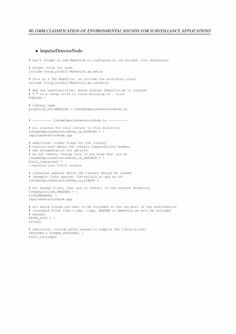
40 GMM CLASSIFICATION OF ENVIRONMENTAL SOUNDS FOR SURVEILLANCE APPLICATIONS
• ImpulseDetectorNode:
# Don’t forget to add Makefile to configure.in (in project root directory)
# helper rules for nasminclude $(top_srcdir)/Makefile.am.extra
# this is a IDL Makefile, so include the according rules!include $(top_srcdir)/Makefile.am.idlextra
# Add any subdirectories, where another Makefile.am is located# "." is a cheap trick to force building of . firstSUBDIRS =
# library namepluginlib_LTLIBRARIES = libnmmImpulseDetectorNode.la
# ---------- libnmmImpulseDetectorNode.la ----------
# all sources for this library in this directorylibnmmImpulseDetectorNode_la_SOURCES = \ImpulseDetectorNode.cpp
# additional linker flags for the library# version-info means the library compatibility number,# see documentation for details# do not remove, change only if you know what you dolibnmmImpulseDetectorNode_la_LDFLAGS = \$(all_libraries) \--version-info 0:0:0 -module
# libraries against which the library should be linked# (example links against libtrallala.so and so on)libnmmImpulseDetectorNode_la_LIBADD =
# all header files, that are to install in the current directorytreepkginclude_HEADERS = \$(IDLHEADERS) \ImpulseDetectorNode.hpp
# all extra things you want to be included in the tar-ball of the distribution# (standard files like *.cpp, *.hpp, README or Makefile.am will be included# anyway)EXTRA_DIST = \$(IDLS)
# additional include paths needed to compile the librar{y,ies}INCLUDES = $(USER_INCLUDES) \$(all_includes)
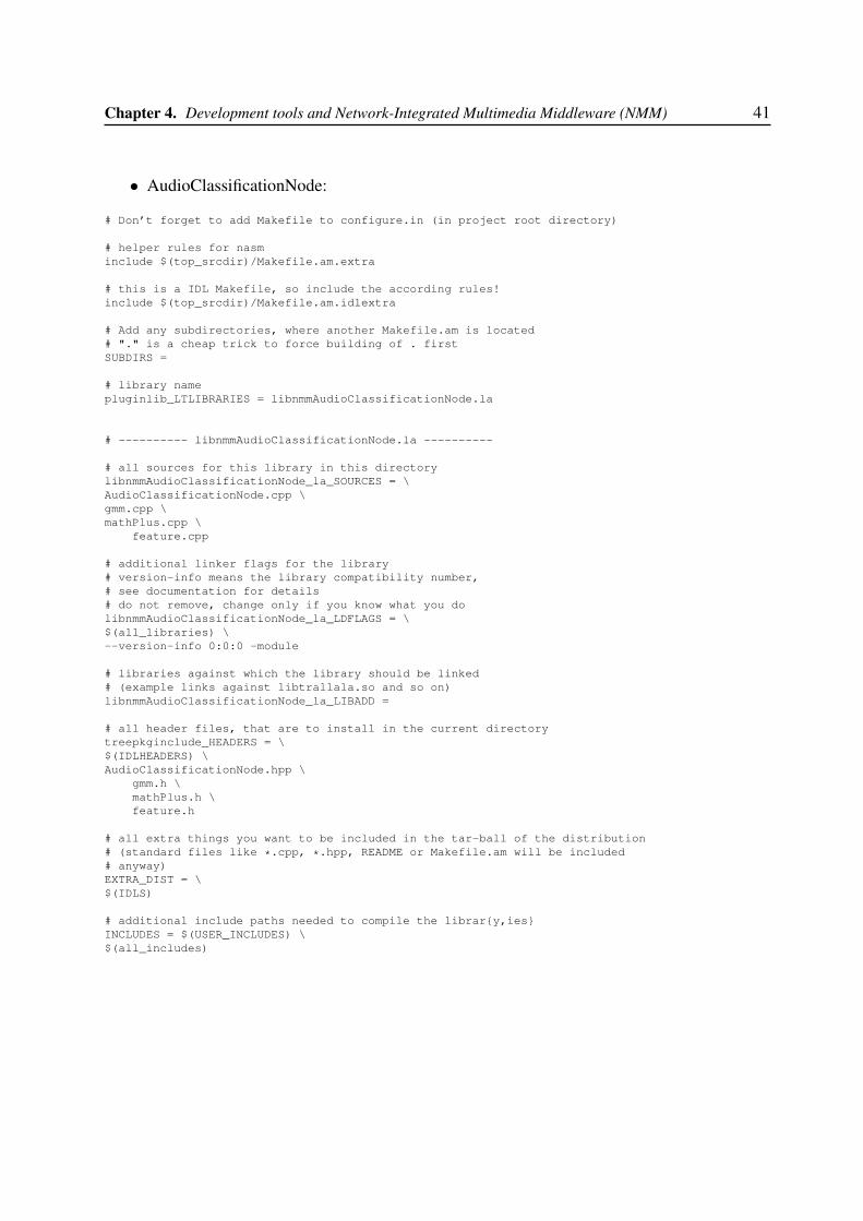
Chapter 4. Development tools and Network-Integrated Multimedia Middleware (NMM) 41
• AudioClassificationNode:
# Don’t forget to add Makefile to configure.in (in project root directory)
# helper rules for nasminclude $(top_srcdir)/Makefile.am.extra
# this is a IDL Makefile, so include the according rules!include $(top_srcdir)/Makefile.am.idlextra
# Add any subdirectories, where another Makefile.am is located# "." is a cheap trick to force building of . firstSUBDIRS =
# library namepluginlib_LTLIBRARIES = libnmmAudioClassificationNode.la
# ---------- libnmmAudioClassificationNode.la ----------
# all sources for this library in this directorylibnmmAudioClassificationNode_la_SOURCES = \AudioClassificationNode.cpp \gmm.cpp \mathPlus.cpp \
feature.cpp
# additional linker flags for the library# version-info means the library compatibility number,# see documentation for details# do not remove, change only if you know what you dolibnmmAudioClassificationNode_la_LDFLAGS = \$(all_libraries) \--version-info 0:0:0 -module
# libraries against which the library should be linked# (example links against libtrallala.so and so on)libnmmAudioClassificationNode_la_LIBADD =
# all header files, that are to install in the current directorytreepkginclude_HEADERS = \$(IDLHEADERS) \AudioClassificationNode.hpp \
gmm.h \mathPlus.h \feature.h
# all extra things you want to be included in the tar-ball of the distribution# (standard files like *.cpp, *.hpp, README or Makefile.am will be included# anyway)EXTRA_DIST = \$(IDLS)
# additional include paths needed to compile the librar{y,ies}INCLUDES = $(USER_INCLUDES) \$(all_includes)
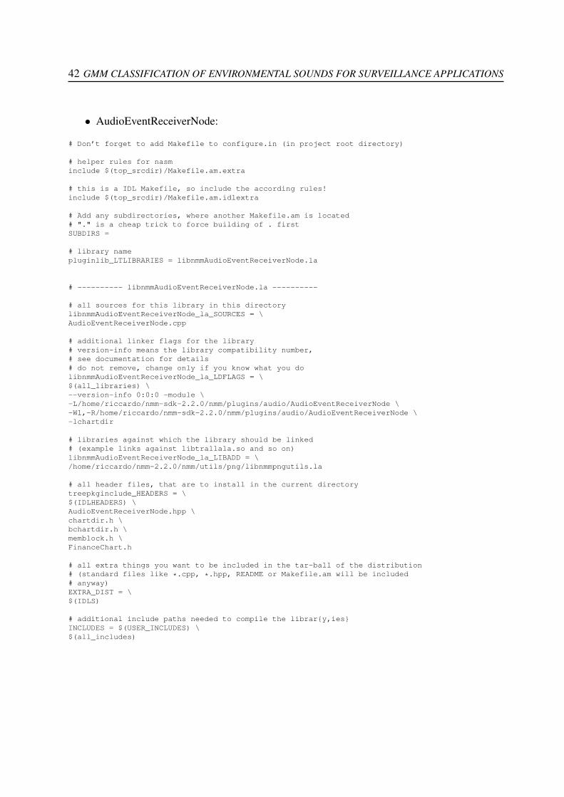
42 GMM CLASSIFICATION OF ENVIRONMENTAL SOUNDS FOR SURVEILLANCE APPLICATIONS
• AudioEventReceiverNode:
# Don’t forget to add Makefile to configure.in (in project root directory)
# helper rules for nasminclude $(top_srcdir)/Makefile.am.extra
# this is a IDL Makefile, so include the according rules!include $(top_srcdir)/Makefile.am.idlextra
# Add any subdirectories, where another Makefile.am is located# "." is a cheap trick to force building of . firstSUBDIRS =
# library namepluginlib_LTLIBRARIES = libnmmAudioEventReceiverNode.la
# ---------- libnmmAudioEventReceiverNode.la ----------
# all sources for this library in this directorylibnmmAudioEventReceiverNode_la_SOURCES = \AudioEventReceiverNode.cpp
# additional linker flags for the library# version-info means the library compatibility number,# see documentation for details# do not remove, change only if you know what you dolibnmmAudioEventReceiverNode_la_LDFLAGS = \$(all_libraries) \--version-info 0:0:0 -module \-L/home/riccardo/nmm-sdk-2.2.0/nmm/plugins/audio/AudioEventReceiverNode \-Wl,-R/home/riccardo/nmm-sdk-2.2.0/nmm/plugins/audio/AudioEventReceiverNode \-lchartdir
# libraries against which the library should be linked# (example links against libtrallala.so and so on)libnmmAudioEventReceiverNode_la_LIBADD = \/home/riccardo/nmm-2.2.0/nmm/utils/png/libnmmpngutils.la
# all header files, that are to install in the current directorytreepkginclude_HEADERS = \$(IDLHEADERS) \AudioEventReceiverNode.hpp \chartdir.h \bchartdir.h \memblock.h \FinanceChart.h
# all extra things you want to be included in the tar-ball of the distribution# (standard files like *.cpp, *.hpp, README or Makefile.am will be included# anyway)EXTRA_DIST = \$(IDLS)
# additional include paths needed to compile the librar{y,ies}INCLUDES = $(USER_INCLUDES) \$(all_includes)
Chapter 5
Experimental Results
5.1 Testing Off-lineTo know the performance of the system, testing off-line is made over the whole database, workingon audio files registered with a microphone. Three test variables are taken into account. Theformer two are boolean, the third is numerical.
1. Noise exclusion on/off. This variable chooses whether to use or not the Noise exclusion (ifset to “off” is not required a noise classification step);
2. Technique of evaluating accuracy smooth/sharp. The simultaneous detection of differentclasses of the same file belonging to one determinate class is evaluated as a correct detec-tion in the smooth accuracy mode, a wrong detection in the sharp accuracy mode;
3. Signal-to-Noise Ratio (SNR). This variable goes from -20 dB to 25 dB with step of 5 dB.
Let N the number of the classes used in the system and C the set of all the classes such thatc1,...,N ∈ C. The performance parameters used are explained in the following:
• True positive: A sound file belonging to a class ci ∈ C and correctly classified in a soundbelonging to the same class ci. TP is the number of true positive files tested;
• False positive: A generic sound file not belonging to any of the classes of C that is wronglyclassified in a sound belonging to some class ci ∈ C. Note that in a multi class systemwith N classes, this parameter incorporates both the prediction that the file that belongs toa class ci ∈ C is wrongly classified in a sound belonging to a class cj ∈ C with j = i, andthe prediction that the audio file that does not belong to any class is wrongly classified in asound belonging to some class ci ∈ C. FP is the number of false positive files tested;
• True negative: A sound file that does not belong to any class ci ∈ C and is not detected bythe system. TN is the number of true negative files tested;
43
44 GMM CLASSIFICATION OF ENVIRONMENTAL SOUNDS FOR SURVEILLANCE APPLICATIONS
• False negative: A sound file belonging to a class ci ∈ C and not classified in any class.FN is the number of false negative files tested.
The accuracy is the proportion of true results (both true positives and true negatives) in adatabase:
Accuracy =TP + TN
TP + FP + FN + TN(5.1)
On the other hand, precision is defined as the proportion of the true positives against all thepositive results (both true positives and false positives):
Precision =TP
TP + FP(5.2)
Accuracy is the degree of veracity while precision is the degree of reproducibility. The anal-ogy used here to explain the difference between accuracy and precision is the target comparison.In this analogy, repeated measurements are compared to arrows that are shot at a target. Accuracydescribes the closeness of arrows to the bullseye at the target center. Arrows that strike closer tothe bullseye are considered more accurate. The closer a system’s measurements to the acceptedvalue, the more accurate the system is considered to be (see Figure 5.1).
Figure 5.1: High accuracy but low precision.
To continue the analogy, if a large number of arrows are shot, precision would be the sizeof the arrow cluster. (When only one arrow is shot, precision is the size of the cluster onewould expect if this were repeated many times under the same conditions.) When all arrowsare grouped tightly together, the cluster is considered precise since they all struck close to thesame spot, even if not necessarily near the bullseye. The measurements are precise, though notnecessarily accurate (see Figure 5.2).
Figure 5.2: High precision but low accuracy.
However, it is not possible to reliably achieve accuracy in individual measurements withoutprecision: if the arrows are not grouped close to one another, they cannot all be close to the

Chapter 5. Experimental Results 45
bullseye (their average position might be an accurate estimation of the bullseye, but the individualarrows are inaccurate).
To increase almost linearly the noise over the clean signals, the background noise was addedto the clean signal changing the NoiseAmplitudeModulation from 0 to 0.9 with 0.1 step.
Unfortunately there is not a good definition of SNR for a set of signals because the audiofiles in the database have different loudness. Our definition of the mean SNR makes sense tocharacterize a real situation where there are audio streams with almost stationary noise, with acertain energy, and various signals with different energies.
SNR’s Average value makes sense because it can be representative of a real situation. EverySNR value reported in the graphs is the mean of the SNRs of all the files referring to the sameNoiseAmplitudeModulation value (the variance has a constant range of ±10 dB). All thefollowing plots are structured in this way: in the x axis there is the mean SNRs and in the y axisthere are the statistical results of accuracy and precision. All data are the mean of 10 iterationsof the accuracy & precision algorithm because the training and the audio test-files constructionare random based.
5.1.1 Global classification performanceHere we show the global performance of the systems with all the four classes of sounds. Thevalues are calculated using all the files of the database for the training of the GMMs. Althoughhere the training set and the test set are the same, the purpose of this analysis is to look at theeffect of noise over the performance. In Figure 5.3 the global accuracy decreases as the SNRdecreases. Using the Noise Subtraction it seems that the accuracy does not improve; this meansthat we can avoid to train the GMMs of the noise that varies according to the place in whichwe want to install the system.
Figure 5.3: Accuracy of all the classes.
From Figure 5.4 we can observe that the whole system is very precise also when there is alow SNR. Obviously, using the restrictive mode, the accuracy and the precision are lower; this is
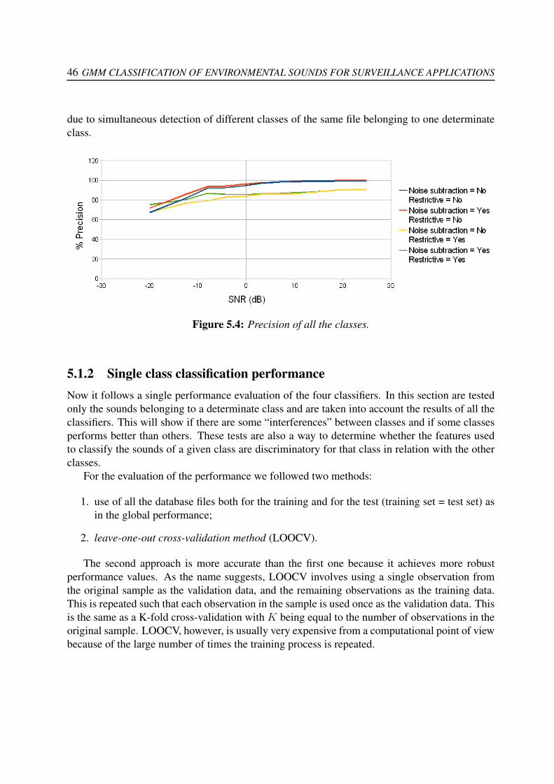
46 GMM CLASSIFICATION OF ENVIRONMENTAL SOUNDS FOR SURVEILLANCE APPLICATIONS
due to simultaneous detection of different classes of the same file belonging to one determinateclass.
Figure 5.4: Precision of all the classes.
5.1.2 Single class classification performanceNow it follows a single performance evaluation of the four classifiers. In this section are testedonly the sounds belonging to a determinate class and are taken into account the results of all theclassifiers. This will show if there are some “interferences” between classes and if some classesperforms better than others. These tests are also a way to determine whether the features usedto classify the sounds of a given class are discriminatory for that class in relation with the otherclasses.
For the evaluation of the performance we followed two methods:
1. use of all the database files both for the training and for the test (training set = test set) asin the global performance;
2. leave-one-out cross-validation method (LOOCV).
The second approach is more accurate than the first one because it achieves more robustperformance values. As the name suggests, LOOCV involves using a single observation fromthe original sample as the validation data, and the remaining observations as the training data.This is repeated such that each observation in the sample is used once as the validation data. Thisis the same as a K-fold cross-validation with K being equal to the number of observations in theoriginal sample. LOOCV, however, is usually very expensive from a computational point of viewbecause of the large number of times the training process is repeated.
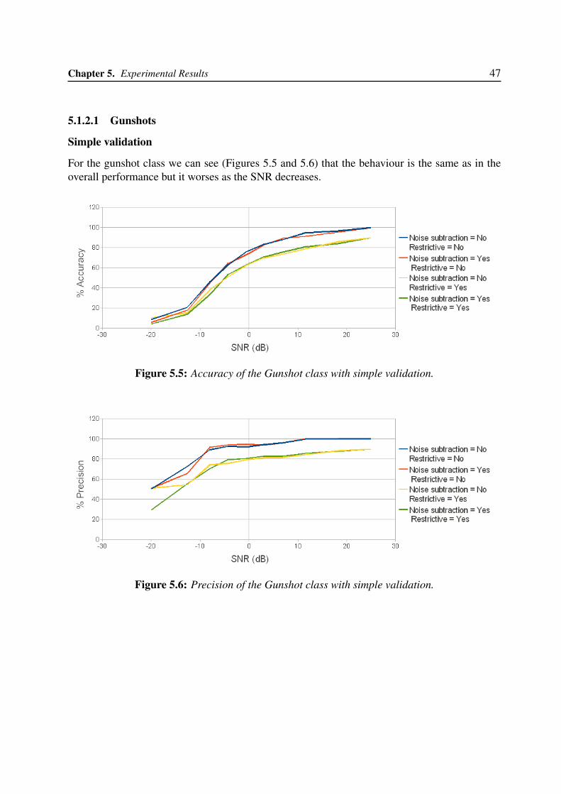
Chapter 5. Experimental Results 47
5.1.2.1 Gunshots
Simple validation
For the gunshot class we can see (Figures 5.5 and 5.6) that the behaviour is the same as in theoverall performance but it worses as the SNR decreases.
Figure 5.5: Accuracy of the Gunshot class with simple validation.
Figure 5.6: Precision of the Gunshot class with simple validation.
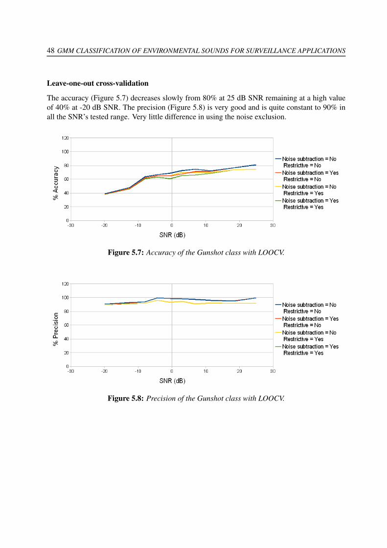
48 GMM CLASSIFICATION OF ENVIRONMENTAL SOUNDS FOR SURVEILLANCE APPLICATIONS
Leave-one-out cross-validation
The accuracy (Figure 5.7) decreases slowly from 80% at 25 dB SNR remaining at a high valueof 40% at -20 dB SNR. The precision (Figure 5.8) is very good and is quite constant to 90% inall the SNR’s tested range. Very little difference in using the noise exclusion.
Figure 5.7: Accuracy of the Gunshot class with LOOCV.
Figure 5.8: Precision of the Gunshot class with LOOCV.
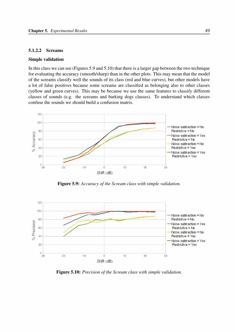
Chapter 5. Experimental Results 49
5.1.2.2 Screams
Simple validation
In this class we can see (Figures 5.9 and 5.10) that there is a larger gap between the two techniquefor evaluating the accuracy (smooth/sharp) than in the other plots. This may mean that the modelof the screams classify well the sounds of its class (red and blue curves), but other models havea lot of false positives because some screams are classified as belonging also to other classes(yellow and green curves). This may be because we use the same features to classify differentclasses of sounds (e.g. the screams and barking dogs classes). To understand which classesconfuse the sounds we should build a confusion matrix.
Figure 5.9: Accuracy of the Scream class with simple validation.
Figure 5.10: Precision of the Scream class with simple validation.
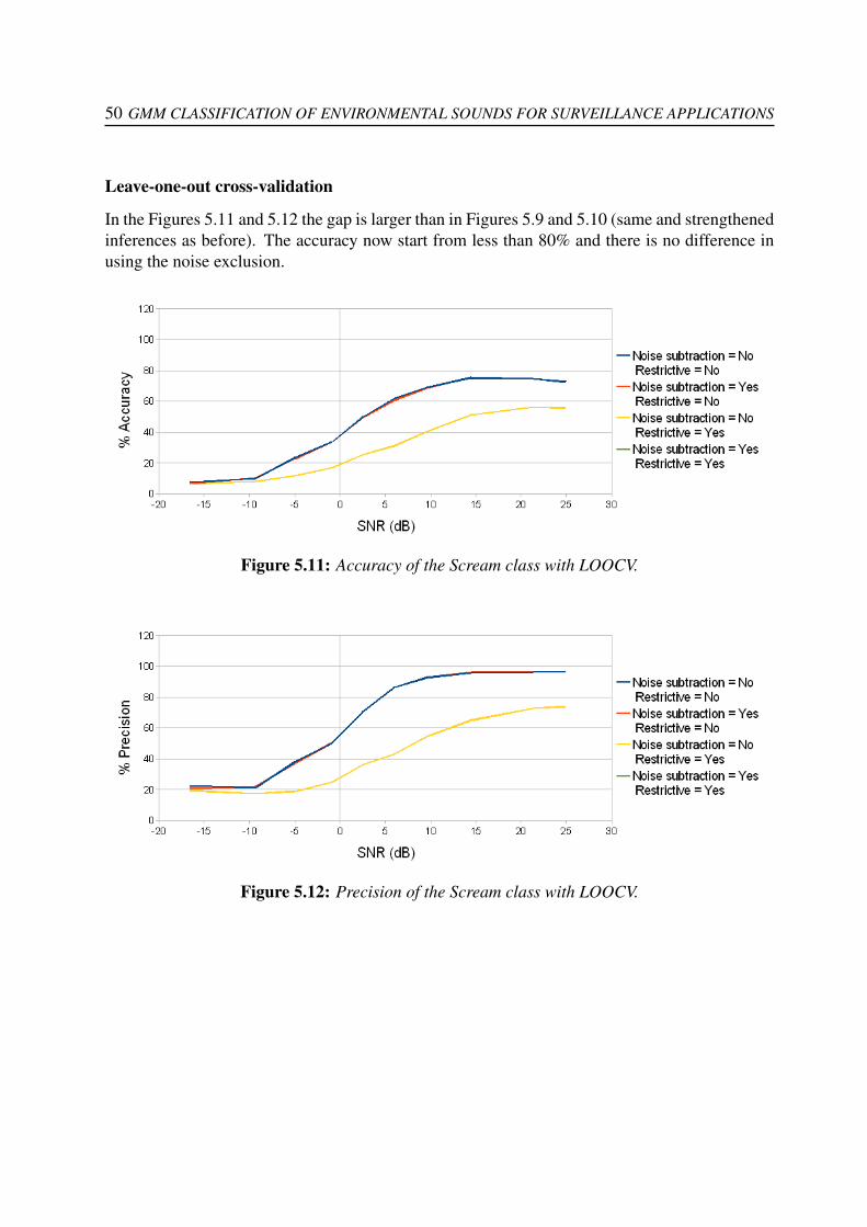
50 GMM CLASSIFICATION OF ENVIRONMENTAL SOUNDS FOR SURVEILLANCE APPLICATIONS
Leave-one-out cross-validation
In the Figures 5.11 and 5.12 the gap is larger than in Figures 5.9 and 5.10 (same and strengthenedinferences as before). The accuracy now start from less than 80% and there is no difference inusing the noise exclusion.
Figure 5.11: Accuracy of the Scream class with LOOCV.
Figure 5.12: Precision of the Scream class with LOOCV.
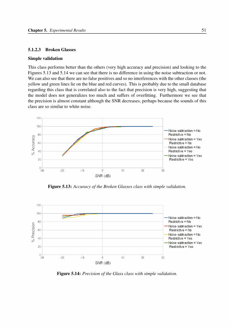
Chapter 5. Experimental Results 51
5.1.2.3 Broken Glasses
Simple validation
This class performs better than the others (very high accuracy and precision) and looking to theFigures 5.13 and 5.14 we can see that there is no difference in using the noise subtraction or not.We can also see that there are no false positives and so no interferences with the other classes (theyellow and green lines lie on the blue and red curves). This is probably due to the small databaseregarding this class that is correlated also to the fact that precision is very high, suggesting thatthe model does not generalizes too much and suffers of overfitting. Furthermore we see thatthe precision is almost constant although the SNR decreases, perhaps because the sounds of thisclass are so similar to white noise.
Figure 5.13: Accuracy of the Broken Glasses class with simple validation.
Figure 5.14: Precision of the Glass class with simple validation.
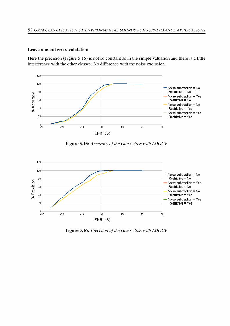
52 GMM CLASSIFICATION OF ENVIRONMENTAL SOUNDS FOR SURVEILLANCE APPLICATIONS
Leave-one-out cross-validation
Here the precision (Figure 5.16) is not so constant as in the simple valuation and there is a littleinterference with the other classes. No difference with the noise exclusion.
Figure 5.15: Accuracy of the Glass class with LOOCV.
Figure 5.16: Precision of the Glass class with LOOCV.

Chapter 5. Experimental Results 53
5.1.2.4 Barking dogs
Simple validation
This class performs quite well with medium high SNRs. With low SNRs accuracy and preci-sion go to zero. With negative SNRs, the lines of the two different techniques of evaluation(smooth/sharp) have the same behaviour, suggesting that other classes does not wrongly detectbarks as sounds of their class.
Figure 5.17: Accuracy of the Barking dogs class with simple validation.
Figure 5.18: Precision of the Bark class with simple validation.
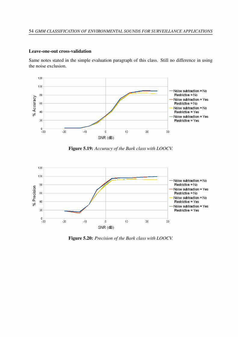
54 GMM CLASSIFICATION OF ENVIRONMENTAL SOUNDS FOR SURVEILLANCE APPLICATIONS
Leave-one-out cross-validation
Same notes stated in the simple evaluation paragraph of this class. Still no difference in usingthe noise exclusion.
Figure 5.19: Accuracy of the Bark class with LOOCV.
Figure 5.20: Precision of the Bark class with LOOCV.
Chapter 5. Experimental Results 55
5.2 Testing Real-timeThe testing of the system in real-time is made using a sound card, a microphone and a loudspeaker (see 4.1.3). For logistical reasons, we lacked spaces with stable conditions of backgroundnoise. Tests were made in the Robotics Lab of DEI/O in Padova. The microphone records aquite constant or stationary background noise with constant energy with added audio events withdifferent energies. So the mean SNR can be considered the mean value of the noise. This valuecharacterizes the noise with one value. Unfortunately it is impossible to calculate the accuracyand the precision of the system in real-time for the difficulty of calculating the SNRs. So, in thissection, we will give only a qualitative accuracy.
5.2.1 Classification performanceTest were divided depending on the type of the source:
1. loud speaker - that plays the audio tests (The microphone is directed towards the speaker);
2. voice and firecrackers - that generate screams and simulate gunshots.
For the first type of source, the quality of the system remains with good performance havingsome volume problems because the features are a bit dependent on the frequency and volume.In fact, directing the microphone towards the tweeter of the speaker, the broken glasses classachieved better performance; while a low volume sound, played by the speaker, was not detected.
For the second type of source the classifier performed worse, due mainly to the fact that thedatabase is small.
Furthermore it should be studied the effect of the reverberation in the room and the conse-quences of it on the system because it caused some problems during the classification step.
5.2.2 Impulse detection performanceThe impulse detector accuracy depends directly on the gain and volume of the microphone andconsequently to the threshold used to detect the impulse. When installing the microphone, thisparameter has to be set to a value that allows the system to detect low volume impulse soundsmaking some tests in the environment. Once set the “volume” threshold to a value, most of theimpulsive sounds that overcome the threshold will be detected because we apply only a simplethreshold condition followed by another tight temporal condition that prevents some sporadicisolated peaks of the signal.


Chapter 6
Conclusions and further work
This project achieves a good off-line classification of the environmental sound taken in consid-eration (gunshots, screams, broken glasses and barking dogs) reaching still 70% of accuracy and90% of precision at 0 dB SNR, starting from 100% of both accuracy and precision with cleansounds at 20 dB SNR.
During the classification the noise exclusion step can be omitted because it does not improvethe performance (e.g. see Figure 5.11). This means that the overhead can be optimized and thatour system does not require a training step for training of the environmental noise. This canbe a winning feature for a future industrial product that does not require a particular set-up thatdepends from the environmental background noise.
The detection of an impulsive sound is made with only one simple feature and has a veryhigh precision and accuracy according obviously to the volume threshold used.
Now we suggest some other works and hints that we have not developed for lack of time butwe think that they can improve the system:
• to enlarge the database. To achieve a more generic classifier for every audio class there isthe need to have a very large database;
• to investigate how much to cut (a formula or a handmade cut ?) the beginning and the tailof the files of the database in order to keep the true “essence” of the audio files of eachclass;
• feature selection. To improve the classification step, the features that best describe eachclass should be identified and selected through a more rigorous feature selection stage,using e.g. principal component analysis (PCA) or other statistical methods;
• to find the best local optimum of the GMMs with repeated iterations of the GMM algorithm- both more iterations of the EM step (now they are 300) and more restarts of the algorithmto avoid falling into a local optimum. This also will improve the classification step;
• to classify more sound classes. Adding a new class is very simple (it requires only theconstruction of the GMM of the class) and does not affect in any way the classifier (itrequires only an insertion of an additional case in the possible outputs of the classifier);
57

58 GMM CLASSIFICATION OF ENVIRONMENTAL SOUNDS FOR SURVEILLANCE APPLICATIONS
• to create a confusion matrix to know how much the models are separated;
• to improve the classification’s validation step using k-folds with a larger database;
• to implement an adaptive threshold for the impulse detector as suggested in [12];
• localization of the sound with arrays of microphones; this will provide more info to thesurveillance system;
• study of the environmental effects (e.g. reverberation) and possible improvements (e.g.dereverberation).

APPENDIX
59

Appendix A
Libraries for the installation of NMM
• a52dec - AC3 audio decoder;
• faad - Decoder for AAC;
• ffmpeg - Various audio and video codecs;
• l1394 - Management of IEEE1394 devices,
• libmp3lame - MPEG layer3 audio encoder;
• libraw1394 - Low level IEEE1394 support;
• libmad - MPEG layer3 audio decoder;
• libdvdnav - DVD reading and navigation;
• libdvdread - DVD reading;
• libogg - OGG file parser;
• libvorbis - OGG/Vorbis audio decoder;
• libshout - Injection of audio streams into a ShoutCast server;
• fftw - Fast Fourier Transformation, used for audio visualization;
• libliveMedia - RTP support;
• mpeg2dec - MPEG version 1/2 video decoder;
• cdparanoia - CDDA Support for Linux.
• libpng - PNG file reader;
• asoundlib - ALSA headers and library;
61
62 GMM CLASSIFICATION OF ENVIRONMENTAL SOUNDS FOR SURVEILLANCE APPLICATIONS
• Xlib - X11 headers and libraries;
• libjpeg - JPEG Support;
• ImageMagick - Imaging Support;
• mplayer - Parts of the implementation of DirectXDisplayNode is based on MPlayer;
• vlc - Parts of the implementation of DirectXDisplayNode is based on vlc;
• transcode - Parts of the C implementation of deinterlacing algorithm in YUVDeInterla-ceNode;
• ogmtools - Parts of the implementation of OGMDemuxNode is taken from the ogmtoolspackage;
• libxmlpp - Some optional plug-ins and features of NMM use a modified version of libxml++,which is provided along with NMM;
• libx264 - H264 encoding support. Used by FFMpegEncodeNode;
• DVB API 5.1 - DVBS2ReadNode depends requires DVB API 5.1, which is part of theLinux kernel headers;
• ulxmlrpcpp - XML-RPC library used by example client of TVCaster using XML-RPCAPI;
• openssl - Dependency of ulxmlrpcpp;
• expat - Dependency of ulxmlrpcpp.

Chapter A. Libraries for the installation of NMM 63
A.1 Informations on external librariesHere is the tables’ legend:
Name The original package name of the libraryDescription A brief description of the libraryVersion The version of the library which works with NMM.
NMM may or may not be be compatible with newer versions of the library.If a custom version of the library is required, then this is indicated here.
Homepage The official project homepage of the external librarySource Name of the package which contains the full source code of the
external library as well asbuild files required to build the library on all supported platforms.The package is either an original source package of the library or a customizedsource package which is based on an original source package.
Binary List of platforms for which precompiled binaries of the library are provided.Licence The type of licence under which the external library is available.
For custom licences (i.e. licences other than the well-known GNU licences),the full licence text is provided in this documentation.
Build Instructions Instructions to build the library from provided sources and build fileson all the platforms
A.1.1 a52decName a52decDescription AC3 audio decoderVersion 0.7.4Homepage http://liba52.sourceforge.net/Source tar.gzBinary Linux, PS3, Mac OS X, WindowsLicence GNU GENERAL PUBLIC LICENCE Version 2
Build Instructions:
tar xzf a52dec-0.7.4.tar.gzcd a52dec-0.7.4./configure --enable-shared --disable-staticmakemake install
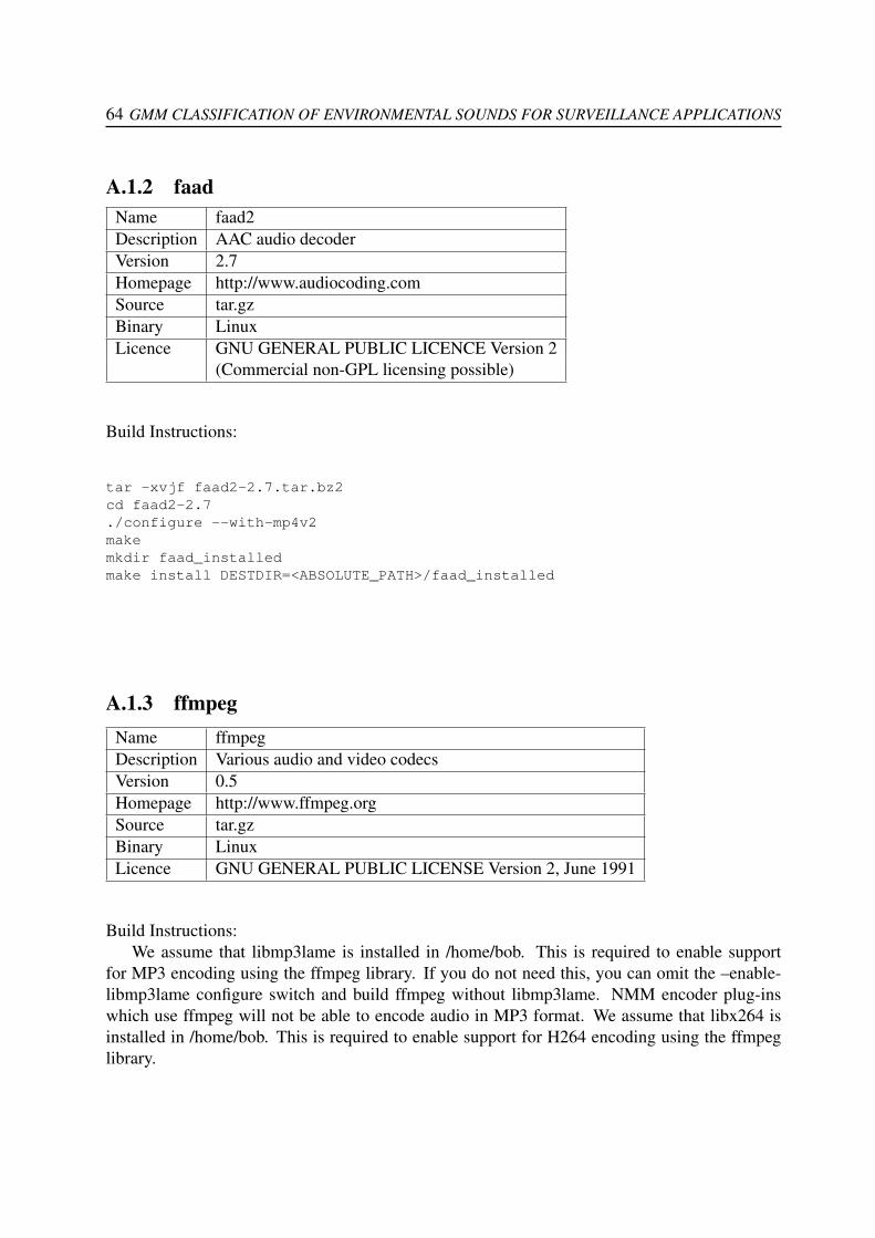
64 GMM CLASSIFICATION OF ENVIRONMENTAL SOUNDS FOR SURVEILLANCE APPLICATIONS
A.1.2 faadName faad2Description AAC audio decoderVersion 2.7Homepage http://www.audiocoding.comSource tar.gzBinary LinuxLicence GNU GENERAL PUBLIC LICENCE Version 2
(Commercial non-GPL licensing possible)
Build Instructions:
tar -xvjf faad2-2.7.tar.bz2cd faad2-2.7./configure --with-mp4v2makemkdir faad_installedmake install DESTDIR=<ABSOLUTE_PATH>/faad_installed
A.1.3 ffmpegName ffmpegDescription Various audio and video codecsVersion 0.5Homepage http://www.ffmpeg.orgSource tar.gzBinary LinuxLicence GNU GENERAL PUBLIC LICENSE Version 2, June 1991
Build Instructions:We assume that libmp3lame is installed in /home/bob. This is required to enable support
for MP3 encoding using the ffmpeg library. If you do not need this, you can omit the –enable-libmp3lame configure switch and build ffmpeg without libmp3lame. NMM encoder plug-inswhich use ffmpeg will not be able to encode audio in MP3 format. We assume that libx264 isinstalled in /home/bob. This is required to enable support for H264 encoding using the ffmpeglibrary.
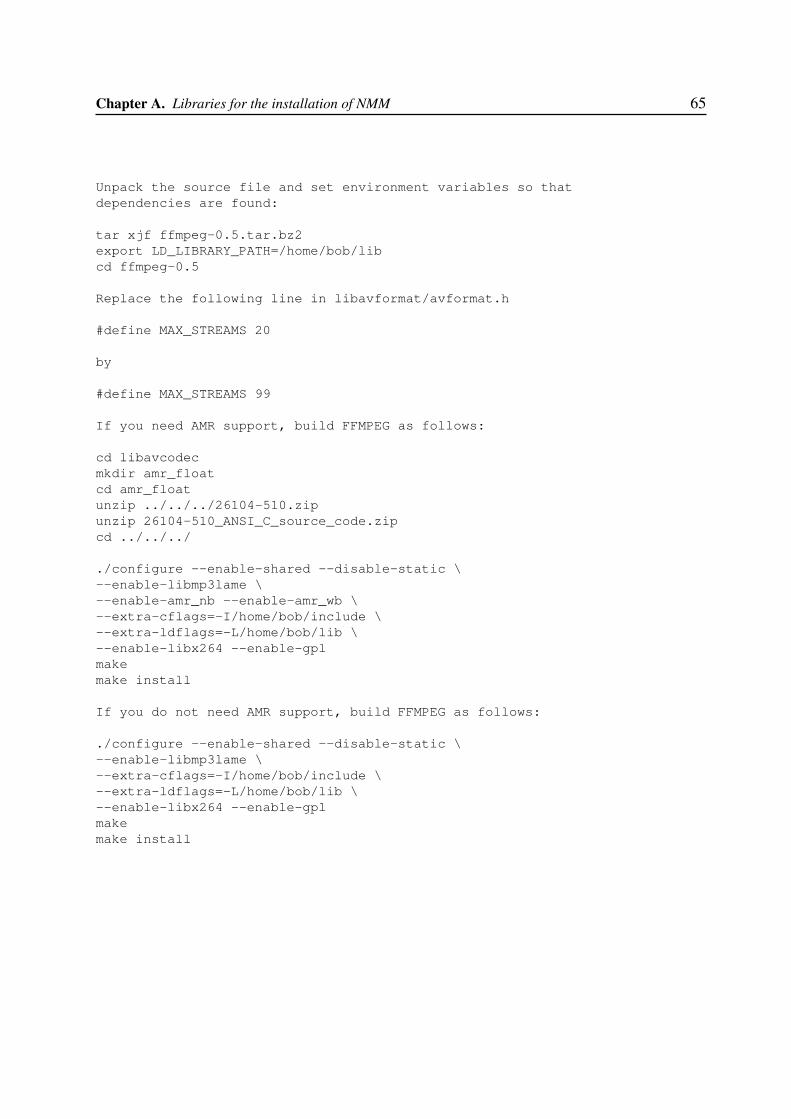
Chapter A. Libraries for the installation of NMM 65
Unpack the source file and set environment variables so thatdependencies are found:
tar xjf ffmpeg-0.5.tar.bz2export LD_LIBRARY_PATH=/home/bob/libcd ffmpeg-0.5
Replace the following line in libavformat/avformat.h
#define MAX_STREAMS 20
by
#define MAX_STREAMS 99
If you need AMR support, build FFMPEG as follows:
cd libavcodecmkdir amr_floatcd amr_floatunzip ../../../26104-510.zipunzip 26104-510_ANSI_C_source_code.zipcd ../../../
./configure --enable-shared --disable-static \--enable-libmp3lame \--enable-amr_nb --enable-amr_wb \--extra-cflags=-I/home/bob/include \--extra-ldflags=-L/home/bob/lib \--enable-libx264 --enable-gplmakemake install
If you do not need AMR support, build FFMPEG as follows:
./configure --enable-shared --disable-static \--enable-libmp3lame \--extra-cflags=-I/home/bob/include \--extra-ldflags=-L/home/bob/lib \--enable-libx264 --enable-gplmakemake install
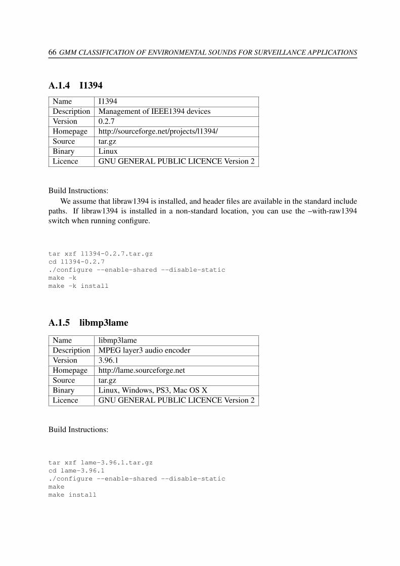
66 GMM CLASSIFICATION OF ENVIRONMENTAL SOUNDS FOR SURVEILLANCE APPLICATIONS
A.1.4 I1394Name I1394Description Management of IEEE1394 devicesVersion 0.2.7Homepage http://sourceforge.net/projects/l1394/Source tar.gzBinary LinuxLicence GNU GENERAL PUBLIC LICENCE Version 2
Build Instructions:We assume that libraw1394 is installed, and header files are available in the standard include
paths. If libraw1394 is installed in a non-standard location, you can use the –with-raw1394switch when running configure.
tar xzf l1394-0.2.7.tar.gzcd l1394-0.2.7./configure --enable-shared --disable-staticmake -kmake -k install
A.1.5 libmp3lame
Name libmp3lameDescription MPEG layer3 audio encoderVersion 3.96.1Homepage http://lame.sourceforge.netSource tar.gzBinary Linux, Windows, PS3, Mac OS XLicence GNU GENERAL PUBLIC LICENCE Version 2
Build Instructions:
tar xzf lame-3.96.1.tar.gzcd lame-3.96.1./configure --enable-shared --disable-staticmakemake install
Chapter A. Libraries for the installation of NMM 67
A.1.6 libraw1394Name libraw1394Description Low level IEEE1394 supportVersion as provided by SuSE 11.0Homepage http://sourceforge.net/projects/libraw1394Binary version abailable noLicence GNU LESSER GENERAL PUBLIC LICENCE Version 2.1
A.1.7 libmadName libmadDescription MPEG layer3 audio decoderVersion 0.15.1bHomepage http://www.underbit.com/products/mad/Source tar.gzBinary Linux, Windows, PS3, Mac OS XLicence GNU GENERAL PUBLIC LICENCE Version 2
Build Instructions:
tar xzf libmad-0.15.1b.tar.gzcd libmad-0.15.1b/./configure --enable-shared --disable-staticmakemake install
A.1.8 libdvdnavName libdvdnavDescription DVD reading and navigationVersion 0.10.1Homepage http://dvd.sourceforge.net/Source tar.gzBinary Linux, Windows, PS3, Mac OS XLicence GNU GENERAL PUBLIC LICENCE Version 2

68 GMM CLASSIFICATION OF ENVIRONMENTAL SOUNDS FOR SURVEILLANCE APPLICATIONS
Build Instructions:
tar xzf libdvdnav-0.1.10.tar.gzcd libdvdnav-0.1.10./configure --enable-shared --disable-staticmakemake install
A.1.9 libdvdreadName libdvdreadDescription DVD readingVersion 0.9.4Homepage http://www.dtek.chalmers.se/groups/dvd/Source tar.gzBinary LinuxLicence GNU GENERAL PUBLIC LICENCE Version 2
Build Instructions:
tar xzf libdvdread-0.9.4.tar.gzcd libdvdread-0.9.4/./configure --enable-shared --disable-staticmakemake install
A.1.10 liboggName liboggDescription OGG file parserVersion 1.1Homepage http://xiph.org/ogg/Source tar.gzBinary LinuxLicence GNU GENERAL PUBLIC LICENCE Version 2
Build Instructions:
tar xzf libogg-1.1.tar.gzcd libogg-1.1
Chapter A. Libraries for the installation of NMM 69
./configure --enable-shared --disable-staticmakemake install
A.1.11 libvorbisName libvorbisDescription OGG/Vorbis audio decoderVersion 1.0.1Homepage http://xiph.org/vorbis/Source tar.gzBinary LinuxLicence GNU GENERAL PUBLIC LICENCE Version 2
Build Instructions:
tar xzf libvorbis-1.0.1.tar.gzcd libvorbis-1.0.1./configure --enable-shared --disable-static --with-ogg=/home/bobmake -kmake -k install
A.1.12 libshoutName libshoutDescription Injection of audio streams into a ShoutCast serverVersion 2.0Homepage http://www.icecast.org/Source tar.gzBinary LinuxLicence GNU GENERAL PUBLIC LICENCE Version 2
Build Instructions:
tar xzf libshout-2.0.tar.gzcd libshout-2.0./configure --enable-shared --disable-static --with-ogg=/home/bob--with-vorbis=/home/bobmakemake install
70 GMM CLASSIFICATION OF ENVIRONMENTAL SOUNDS FOR SURVEILLANCE APPLICATIONS
A.1.13 fftwName fftwDescription Fast Fourier Transformation, used for audio visualizationVersion 2.1.5Homepage http://www.fftw.org/Source tar.gzBinary LinuxLicence GNU GENERAL PUBLIC LICENCE Version 2
Build Instructions:
tar xzf fftw-2.1.5.tar.gzcd fftw-2.1.5./configure --enable-shared --disable-staticmakemake install
A.1.14 libliveMediaName libliveMediaDescription RTP supportVersion 2009.06.02 with modifications by MotamaHomepage http://live555.com/liveMedia/Source tar.gzBinary Linux, WindowsLicence GNU LESSER GENERAL PUBLIC LICENCE Version 2.1
Build Instructions:
# Unpacktar xzf live.2009.06.02.tar.gzcd live
# Add -DUSE_SYSTEM_RANDOM to COMPILE_OPTS in config.linux (to avoid segfault)
# Build static libraries./genMakefiles linuxmake
# Build shared librarygcc -shared -o libliveMedia.so.2009.06.02 */*.aln -s libliveMedia.so.2009.06.02 libliveMedia.so
Chapter A. Libraries for the installation of NMM 71
# install to \$INSTALLDIRfind -name \*.hh -exec cp "{}" \$INSTALLDIR/include/live ";"find -name \*.h -exec cp "{}" \$INSTALLDIR/include/live ";"cp libliveMedia.so.2009.06.02 libliveMedia.so \$INSTALLDIR/lib
Build Instructions (Windows):
Open Microsoft Visual Studio 2005.
Unpack the file live.2005.07.13.tar.gz.
Open the solution file liveMedia.sln from the source package.
In the combo box for selecting the build configuration, pick Release.
Choose "Build Solution" from the "Build" menu
Copy the DLL file from the Release directory to a directory that islisted in your PATH environment variable.This is required for running NMM-based applications that use this library.
Copy the LIB file from the Release directory to a directory that is listed asadditional library directory in your Visual Studio project files that use thisexternal library.(This is only required for development of applications that use thislibrary directly.You may not need to do this at all.)
A.1.15 mpeg2dec
Name mpeg2decDescription MPEG version 1/2 video decoderVersion 0.4.0bHomepage http://libmpeg2.sourceforge.net/Source tar.gzBinary Linux, Windows, Mac OsXLicence GNU GENERAL PUBLIC LICENSE Version 2
Build Instructions:
tar xzf mpeg2dec-0.4.0b.tar.gzcd mpeg2dec-0.4.0/./configure --enable-shared --disable-staticmakemake install
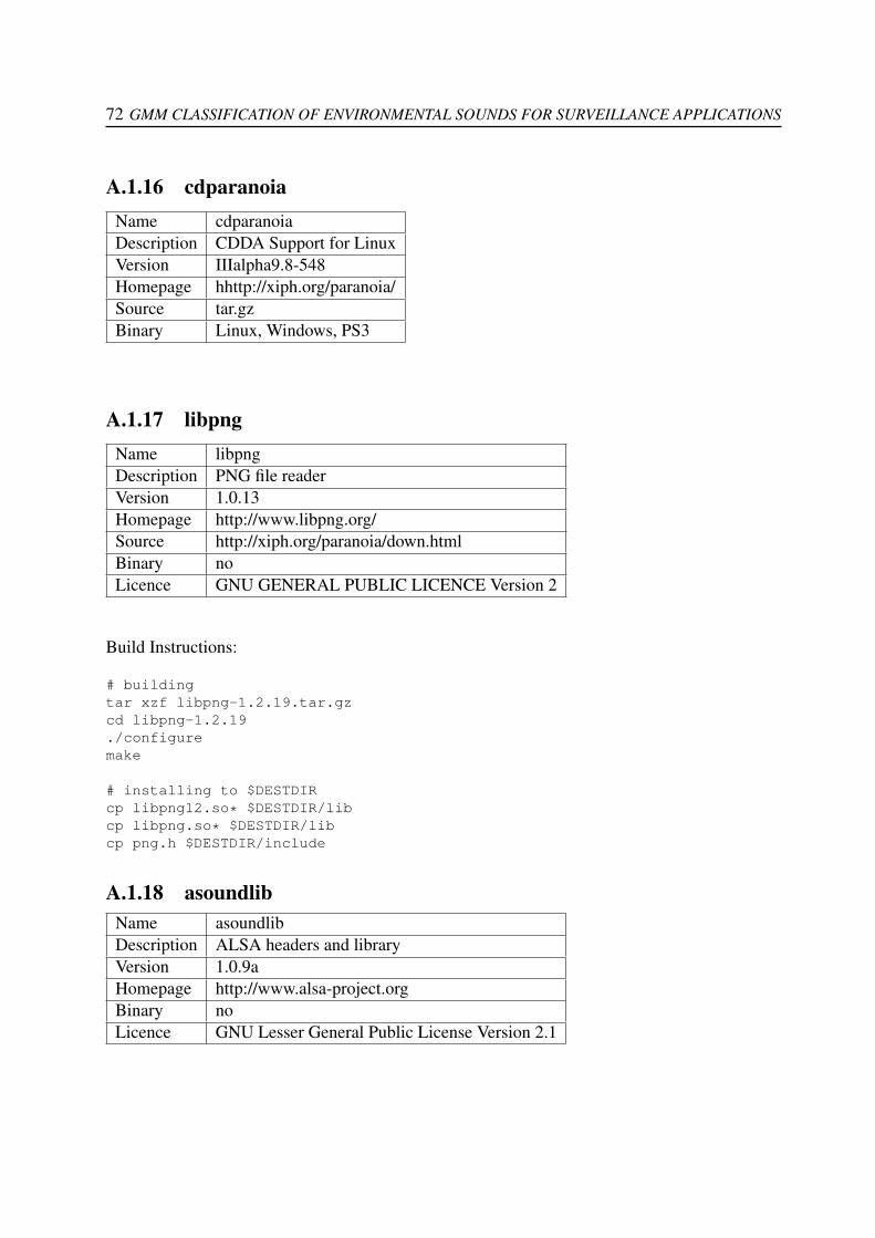
72 GMM CLASSIFICATION OF ENVIRONMENTAL SOUNDS FOR SURVEILLANCE APPLICATIONS
A.1.16 cdparanoiaName cdparanoiaDescription CDDA Support for LinuxVersion IIIalpha9.8-548Homepage hhttp://xiph.org/paranoia/Source tar.gzBinary Linux, Windows, PS3
A.1.17 libpngName libpngDescription PNG file readerVersion 1.0.13Homepage http://www.libpng.org/Source http://xiph.org/paranoia/down.htmlBinary noLicence GNU GENERAL PUBLIC LICENCE Version 2
Build Instructions:
# buildingtar xzf libpng-1.2.19.tar.gzcd libpng-1.2.19./configuremake
# installing to $DESTDIRcp libpng12.so* $DESTDIR/libcp libpng.so* $DESTDIR/libcp png.h $DESTDIR/include
A.1.18 asoundlibName asoundlibDescription ALSA headers and libraryVersion 1.0.9aHomepage http://www.alsa-project.orgBinary noLicence GNU Lesser General Public License Version 2.1

Chapter A. Libraries for the installation of NMM 73
A.1.19 Xlib
Name XlibDescription X11 headers and librariesBinary no
A.1.20 libjpeg
Name libjpegDescription JPEG supportVersion 6.2.0-738Homepage http://www.ijg.org/Source http://www.ijg.org/files/Binary PS3
A.1.21 ImageMagick
Name ImageMagickDescription Imaging SupportVersion 6.4.0.4 (as provided with OpenSuSE 11.0)Homepage http://www.imagemagick.orgSource tar.bz2Binary Linux
Build Instructions:
tar xvfz ImageMagick-6.3.5-5.tar.gzcd ImageMagick-6.3.5/./configuremakemake install
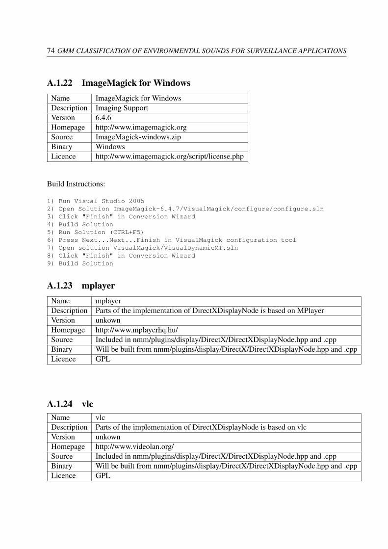
74 GMM CLASSIFICATION OF ENVIRONMENTAL SOUNDS FOR SURVEILLANCE APPLICATIONS
A.1.22 ImageMagick for WindowsName ImageMagick for WindowsDescription Imaging SupportVersion 6.4.6Homepage http://www.imagemagick.orgSource ImageMagick-windows.zipBinary WindowsLicence http://www.imagemagick.org/script/license.php
Build Instructions:
1) Run Visual Studio 20052) Open Solution ImageMagick-6.4.7/VisualMagick/configure/configure.sln3) Click "Finish" in Conversion Wizard4) Build Solution5) Run Solution (CTRL+F5)6) Press Next...Next...Finish in VisualMagick configuration tool7) Open solution VisualMagick/VisualDynamicMT.sln8) Click "Finish" in Conversion Wizard9) Build Solution
A.1.23 mplayerName mplayerDescription Parts of the implementation of DirectXDisplayNode is based on MPlayerVersion unkownHomepage http://www.mplayerhq.hu/Source Included in nmm/plugins/display/DirectX/DirectXDisplayNode.hpp and .cppBinary Will be built from nmm/plugins/display/DirectX/DirectXDisplayNode.hpp and .cppLicence GPL
A.1.24 vlcName vlcDescription Parts of the implementation of DirectXDisplayNode is based on vlcVersion unkownHomepage http://www.videolan.org/Source Included in nmm/plugins/display/DirectX/DirectXDisplayNode.hpp and .cppBinary Will be built from nmm/plugins/display/DirectX/DirectXDisplayNode.hpp and .cppLicence GPL

Chapter A. Libraries for the installation of NMM 75
A.1.25 transcode
Name transcodeDescription Parts of the C implementation of deinterlacing algorithm in YUVDeInterlaceNodeVersion unkownHomepage http://www.transcoding.orgSource Included in nmm/plugins/video/filter/yv12 deinterlace.h and .cBinary Will be built from nmm/plugins/video/filter/yv12 deinterlace.h and .cLicence GPL
A.1.26 ogmtools
Name ogmtoolsDescription Parts of the implementation of OGMDemuxNode is taken from the ogmtools packageVersion unkownHomepage http://www.bunkus.org/videotools/ogmtools/Source nmm/plugins/av/ogm/ogmstreams.hBinary Will be built from sources in nmm/plugins/av/ogmLicence GPL
A.1.27 libxml++
Name libxml++Description Some optional plug-ins and features of NMM use a modified version of libxml++,
which is provided along with NMM.Version unkownHomepage http://libxmlplusplus.sourceforge.net/Source nmm/utils/xmlBinary Will be built from sources in nmm/utils/xmlLicence LGPL
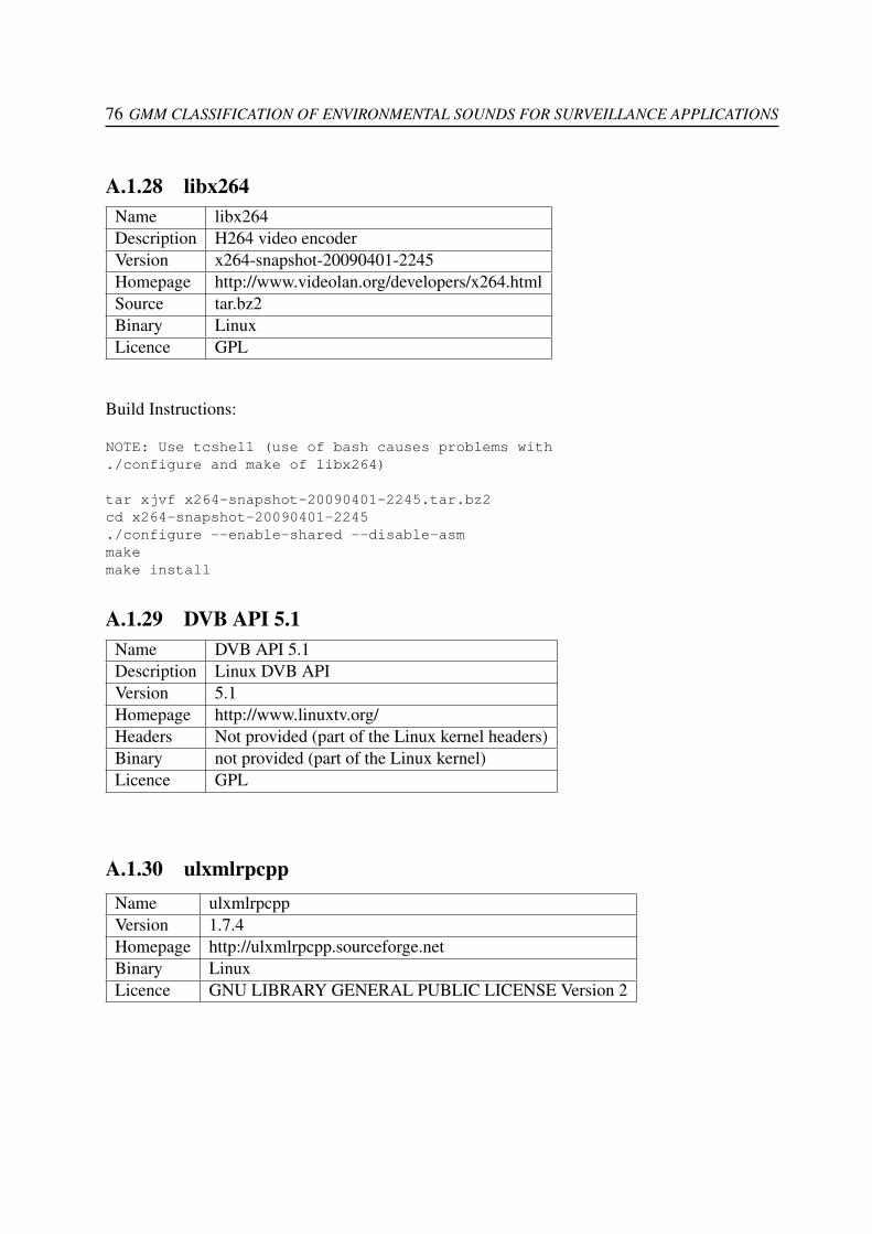
76 GMM CLASSIFICATION OF ENVIRONMENTAL SOUNDS FOR SURVEILLANCE APPLICATIONS
A.1.28 libx264Name libx264Description H264 video encoderVersion x264-snapshot-20090401-2245Homepage http://www.videolan.org/developers/x264.htmlSource tar.bz2Binary LinuxLicence GPL
Build Instructions:
NOTE: Use tcshell (use of bash causes problems with./configure and make of libx264)
tar xjvf x264-snapshot-20090401-2245.tar.bz2cd x264-snapshot-20090401-2245./configure --enable-shared --disable-asmmakemake install
A.1.29 DVB API 5.1Name DVB API 5.1Description Linux DVB APIVersion 5.1Homepage http://www.linuxtv.org/Headers Not provided (part of the Linux kernel headers)Binary not provided (part of the Linux kernel)Licence GPL
A.1.30 ulxmlrpcppName ulxmlrpcppVersion 1.7.4Homepage http://ulxmlrpcpp.sourceforge.netBinary LinuxLicence GNU LIBRARY GENERAL PUBLIC LICENSE Version 2
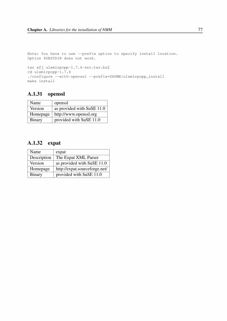
Chapter A. Libraries for the installation of NMM 77
Note: You have to use --prefix option to specify install location.Option $DESTDIR does not work.
tar xfj ulxmlrpcpp-1.7.4-src.tar.bz2cd ulxmlrpcpp-1.7.4./configure --with-openssl --prefix=$HOME/ulxmlrpcpp_installmake install
A.1.31 opensslName opensslVersion as provided with SuSE 11.0Homepage http://www.openssl.orgBinary provided with SuSE 11.0
A.1.32 expatName expatDescription The Expat XML ParserVersion as provided with SuSE 11.0Homepage http://expat.sourceforge.net/Binary provided with SuSE 11.0

Bibliography
[1] G. Valenzise, L. Gerosa, M. Tagliasacchi, F. Antonacci, and A. Sarti. Scream and gunshotdetection and localization for audio-surveillance systems. In Advanced Video and SignalBased Surveillance, 2007. AVSS 2007. IEEE Conference on, pages 21 –26, sep. 2007.
[2] G. Valenzise, L. Gerosa, M. Tagliasacchi, F. Antonacci, and A. Sarti. Scream and gunshotdetection in noisy environments. Dipartimento di Elettronica e Informazione - Politecnicodi Milano.
[3] Marco Cristani, Manuele Bicego, and Vittorio Murino. Audio-visual event recognition insurveillance video sequences. In Multimedia, IEEE Transactions on, volume 9, pages 257–267, feb. 2007.
[4] J.-L. Rouas, J. Louradour, and S. Ambellouis. Audio events detection in public transportvehicle. In Intelligent Transportation Systems Conference, 2006. ITSC ’06. IEEE, pages733 –738, sep. 2006.
[5] C. Clavel, T. Ehrette, and G. Richard. Events detection for an audio-based surveillancesystem. In Multimedia and Expo, 2005. ICME 2005. IEEE International Conference on,pages 1306 –1309, jul. 2005.
[6] A. Dufaux, L. Besacier, M. Ansorge, and F. Pellandini. Automatic sound detection andrecognition for noisy environment. In European Signal Processing Conference (EU-SIPCO), Tampere, Finlande, sep. 2000.
[7] V. Peltonen, J. Tuomi, A. Klapuri, J. Huopaniemi, and T. Sorsa. Computational audi-tory scene recognition. In Acoustics, Speech, and Signal Processing, 2002. Proceedings.(ICASSP ’02). IEEE International Conference on, volume 2, pages 1941 –1944, 2002.
[8] G. Tzanetakis and P. Cook. Musical genre classification of audio signals. In Speech andAudio Processing, IEEE Transactions on, volume 10, pages 293 – 302, jul. 2002.
[9] Rui Cai, Lie Lu, Hong-Jiang Zhang, and Lian-Hong Cai. Highlight sound effects detectionin audio stream. In Multimedia and Expo, 2003. ICME ’03. Proceedings. 2003 Interna-tional Conference on, volume 3, pages III – 37–40 vol.3, jul. 2003.
79
80 GMM CLASSIFICATION OF ENVIRONMENTAL SOUNDS FOR SURVEILLANCE APPLICATIONS
[10] Hoiem D, Yan Ke, and R. Sukthankar. Solar: sound object localization and retrieval incomplex audio environments. In Acoustics, Speech, and Signal Processing, 2005. Proceed-ings. (ICASSP ’05). IEEE International Conference on, volume 5, pages v/429 – v/432 Vol.5, mar. 2005.
[11] P.K. Atrey, N.C. Maddage, and M.S. Kankanhalli. Audio based event detection for mul-timedia surveillance. In Acoustics, Speech and Signal Processing, 2006. ICASSP 2006Proceedings. 2006 IEEE International Conference on, volume 5, pages V –V, may. 2006.
[12] James F. Kaiser. On a simple algorithm to calculate the ‘energy’ of a signal. In ProceedingsICASSP90, pages 381–384, 1990.
[13] Geoffroy Peeters. A large set of audio features for sound description (similarity and classi-fication) in the cuidado project. April 2004.
[14] Stanley Smith Stevens, John Volkman, and Edwin Newman. A scale for the measurementof the psychological magnitude of pitch. In Journal of the Acoustical Society of America,volume 8 (3), page 185190, 1937.
[15] Douglas O’Shaughnessy. Speech communication: human and machine. Addison-Wesleyp. 150, 1987.
[16] Jacob Benesty, M. M. Sondhi, and Yiteng Huang. Springer Handbook of Speech Process-ing. Springer, 2008.
[17] Lie Lu, Hong-Jiang Zhang, and Hao Jiang. Content analysis for audio classification andsegmentation. In Speech and Audio Processing, IEEE Transactions on, volume 10, pages504 – 516, oct. 2002.
[18] Richard O. Duda, Peter E. Hart, and David G. Stork. Pattern Classification. Wiley IndiaPvt. Ltd., second edition, 2007.
[19] The Freesound Project. http://www.freesound.org/.
[20] ChartDirector. http://www.advsofteng.com/.
[21] Motama. Nmm site - http://www.motama.com/nmm.html.