GloptiPoly: Global Optimization over Polynomials

with Matlab and SeDuMi

Didier Henrion1,2, Jean-Bernard Lasserre1

henrion@laas.fr, lasserre@laas.frwww.laas.fr/∼henrion, www.laas.fr/∼lasserre

Version 2.3.0 of December 13, 2006

Abstract

GloptiPoly is a Matlab/SeDuMi add-on to build and solve convex linear matrixinequality relaxations of the (generally non-convex) global optimization problem ofminimizing a multivariable polynomial function subject to polynomial inequality,equality or integer constraints. It generates a series of lower bounds monotonicallyconverging to the global optimum. Global optimality is detected and isolated op-timal solutions are extracted automatically. Numerical experiments show that formost of the small- and medium-scale problems described in the literature, the globaloptimum is reached at low computational cost.

1 Introduction

GloptiPoly is a Matlab utility that builds and solves convex linear matrix inequality (LMI)relaxations of (generally non-convex) global optimization problems with multivariablereal-valued polynomial criterion and constraints. It is based on the theory described in[7, 8]. Related results can be found also in [11] and [12]. GloptiPoly does not intent tosolve non-convex optimization problems globally, but allows to solve a series of convexrelaxations of increasing size, whose optima are guaranteed to converge monotonically tothe global optimum.

GloptiPoly solves LMI relaxations with the help of the solver SeDuMi [13], taking fulladvantage of sparsity and special problem structure. Optionally, a user-friendly inter-face called DefiPoly, based on Matlab Symbolic Math Toolbox, can be used jointly withGloptiPoly to define the optimization problems symbolically with a Maple-like syntax.

GloptiPoly is aimed at small- and medium-scale problems. Numerical experiments illus-trate that for most of the problem instances available in the literature, the global optimumis reached exactly with LMI relaxations of medium size, at a relatively low computationalcost.

1LAAS-CNRS, 7 Avenue du Colonel Roche, 31077 Toulouse, France2Also with the Department of Control Engineering, Faculty of Electrical Engineering, Czech Technical

University in Prague, Technicka 6, 16628 Prague, Czech Republic

1

2 Installation

GloptiPoly requires Matlab version 5.3 or higher [10], together with the freeware solverSeDuMi version 1.05 or higher [13]. Moreover, the Matlab source file gloptipoly.m mustbe installed in the current working directory, see

www.laas.fr/∼henrion/software/gloptipoly

The optional, companion Matlab source files to GloptiPoly, described throughout thismanuscript, can be found at the same location.

3 Getting started

Figure 1: Six-hump camel back function.

Consider the classical problem of minimizing globally the two-dimensional six-hump camelback function [4, Pb. 8.2.5]

f(x1, x2) = x21(4− 2.1x2

1 + x41/3) + x1x2 + x2

2(−4 + 4x22).

The function has six local minima, two of them being global minima, see figure 1.

2

To minimize this function we build the coefficient matrix

P =

0 0 −4 0 40 1 0 0 04 0 0 0 00 0 0 0 0

−2.1 0 0 0 00 0 0 0 0

1/3 0 0 0 0

where each entry (i, j) in P contains the coefficient of the monomial xi

1xj2 in polynomial

f(x1, x2). We invoke GloptiPoly with the following Matlab script:

>> P(1,3) = -4; P(1,5) = 4; P(2,2) = 1;

>> P(3,1) = 4; P(5,1) = -2.1; P(7,1) = 1/3;

>> out = gloptipoly(P);

On our platform, a Sun Blade 100 workstation with 640 Mb of RAM running under SunOS5.8, we obtain the following output:

GloptiPoly 2.0 - Global Optimization over Polynomials with SeDuMiNumber of variables = 2Number of constraints = 0Maximum polynomial degree = 6Order of LMI relaxation = 3Building LMI. Please wait..Number of LMI decision variables = 27Size of LMI constraints = 100Sparsity of LMI constraints = 3.6667% of non-zero entriesNorm of perturbation of criterion = 0Numerical accuracy for SeDuMi = 1e-09No feasibility radiusSolving LMI problem with SeDuMi.....CPU time = 0.61 secLMI criterion = -1.0316Checking relaxed LMI vector with threshold = 1e-06Relaxed vector reaches a criterion of -7.2166e-15Relaxed vector is feasibleDetecting global optimality (rank shift = 1)..Relative threshold for rank evaluation = 0.001Moment matrix of order 1 has size 3 and rank 2Moment matrix of order 2 has size 6 and rank 2Rank condition ensures global optimalityExtracting solutions..Relative threshold for basis detection = 1e-06Maximum relative error = 3.5659e-082 solutions extracted

3

The first field out.status in the output structure indicates that the global minimumwas reached, the criterion at the optimum is equal to out.crit = -1.0316, and the twoglobally optimal solutions are returned in cell array out.sol:

>> out

out =

status: 1

crit: -1.0316

sol: {[2x1 double] [2x1 double]}

>> out.sol{:}

ans =

0.0898

-0.7127

ans =

-0.0898

0.7127

4 GloptiPoly’s input: defining and solving an opti-

mization problem

4.1 Handling constraints. Basic syntax

Consider the concave optimization problem of finding the radius of the intersection ofthree ellipses [5]:

max x21 + x2

2

s.t. 2x21 + 3x2

2 + 2x1x2 ≤ 13x2

1 + 2x22 − 4x1x2 ≤ 1

x21 + 6x2

2 − 4x1x2 ≤ 1.

In order to specify both the objective and the constraint to GloptiPoly, we first transformthe problem into a minimization problem over non-negative constraints, i.e.

min

1x1

x21

T 0 0 −10 0 0−1 0 0

1x2

x22

s.t.

1x1

x21

T 1 0 −30 −2 0−2 0 0

1x2

x22

≥ 0

1x1

x21

T 1 0 −20 4 0−3 0 0

1x2

x22

≥ 0

1x1

x21

T 1 0 −60 4 0−1 0 0

1x2

x22

≥ 0.

4

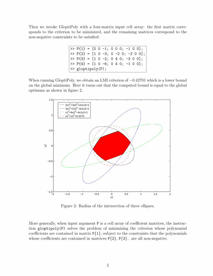
Then we invoke GloptiPoly with a four-matrix input cell array: the first matrix corre-sponds to the criterion to be minimized, and the remaining matrices correspond to thenon-negative constraints to be satisfied:

>> P{1} = [0 0 -1; 0 0 0; -1 0 0];

>> P{2} = [1 0 -3; 0 -2 0; -2 0 0];

>> P{3} = [1 0 -2; 0 4 0; -3 0 0];

>> P{4} = [1 0 -6; 0 4 0; -1 0 0];

>> gloptipoly(P);

When running GloptiPoly, we obtain an LMI criterion of −0.42701 which is a lower boundon the global minimum. Here it turns out that the computed bound is equal to the globaloptimum as shown in figure 2.

−2 −1.5 −1 −0.5 0 0.5 1 1.5 2−1.5

−1

−0.5

0

0.5

1

1.5

x1

x2

2x12+3x22+2x1x2=13x12+2x22−4x1x2=1x12+6x22−4x1x2=1x12+x22=0.4270

Figure 2: Radius of the intersection of three ellipses.

More generally, when input argument P is a cell array of coefficient matrices, the instruc-tion gloptipoly(P) solves the problem of minimizing the criterion whose polynomialcoefficients are contained in matrix P{1}, subject to the constraints that the polynomialswhose coefficients are contained in matrices P{2}, P{3}.. are all non-negative.

5

4.2 Handling constraints. General syntax

To handle directly maximization problems, non-positive inequality or equality constraints,a more explicit but somehow more involved syntax is required. Input argument P mustbe a cell array of structures with fields:

P{i}.c - polynomial coefficient matrices;

P{i}.t - identification string, either

’min’ - criterion to minimize, or

’max’ - criterion to maximize, or

’>=’ - non-negative inequality constraint, or

’<=’ - non-positive inequality constraint, or

’==’ - equality constraint.

For example, if we want to solve the optimization problem [4, Pb. 4.9]

min −12x1 − 7x2 + x22

s.t. −2x41 − x2 + 2 = 0

0 ≤ x1 ≤ 20 ≤ x2 ≤ 3

we use the following script:

>> P{1}.c = [0 -7 1; -12 0 0]; P{1}.t = ’min’;

>> P{2}.c = [2 -1; 0 0; 0 0; 0 0; -2 0]; P{2}.t = ’==’;

>> P{3}.c = [0; -1]; P{3}.t = ’<=’;

>> P{4}.c = [-2; 1]; P{4}.t = ’<=’;

>> P{5}.c = [0 -1]; P{5}.t = ’<=’;

>> P{6}.c = [-3 1]; P{6}.t = ’<=’;

>> gloptipoly(P);

We obtain −16.7389 as the global minimum, with optimal solution x1 = 0.7175 andx2 = 1.4698, see figure 3.

4.3 Sparse polynomial coefficients. Saving memory

When defining optimization problems with a lot of variables or polynomials of high de-grees, the coefficient matrix associated with a polynomial criterion or constraint mayrequire a lot of memory to be stored in Matlab. For example in the case of a quadraticprogram with 10 variables, the number of entries of the coefficient matrix may be as largeas (2 + 1)10 = 59049.

6

0 0.2 0.4 0.6 0.8 1 1.2 1.4 1.6 1.8 20

0.5

1

1.5

2

2.5

3

x1

x 2−35

−31

−31

−27

−27

−27

−23

−23

−23

−19

−19

−19

−15

−15

−15−11

−11

−11

−7

−7−3

Figure 3: Contour plot of −12x1 − 7x2 + x22 with constraint −2x4

1 − x2 + 2 = 0 in dashedline.

An alternative syntax allows to define coefficient matrices of Matlab sparse class. Becausesparse Matlab matrices cannot have more than two dimensions, we store them as sparsecolumn vectors in coefficient field P.c, with an additional field P.s which is the vector ofdimensions of the coefficient matrix, as returned by Matlab function size if the matrixwere not sparse.

For example, to define the quadratic criterion

min10∑i=1

ix2i

the instructions

>> P.c(3,1,1,1,1,1,1,1,1,1) = 1;

>> P.c(1,3,1,1,1,1,1,1,1,1) = 2;

...

>> P.c(1,1,1,1,1,1,1,1,1,3) = 10;

would create a 10-dimensional matrix P.c requiring 472392 bytes for storage. The equiv-alent instructions

7

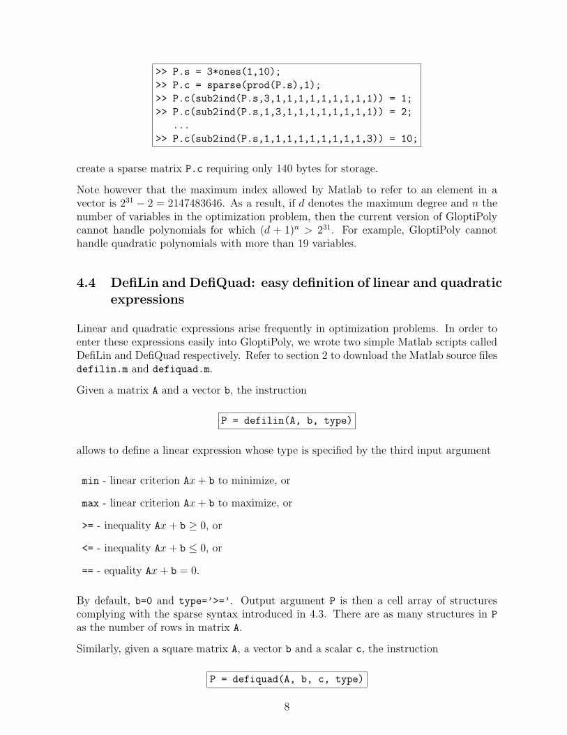
>> P.s = 3*ones(1,10);

>> P.c = sparse(prod(P.s),1);

>> P.c(sub2ind(P.s,3,1,1,1,1,1,1,1,1,1)) = 1;

>> P.c(sub2ind(P.s,1,3,1,1,1,1,1,1,1,1)) = 2;

...

>> P.c(sub2ind(P.s,1,1,1,1,1,1,1,1,1,3)) = 10;

create a sparse matrix P.c requiring only 140 bytes for storage.

Note however that the maximum index allowed by Matlab to refer to an element in avector is 231 − 2 = 2147483646. As a result, if d denotes the maximum degree and n thenumber of variables in the optimization problem, then the current version of GloptiPolycannot handle polynomials for which (d + 1)n > 231. For example, GloptiPoly cannothandle quadratic polynomials with more than 19 variables.

4.4 DefiLin and DefiQuad: easy definition of linear and quadraticexpressions

Linear and quadratic expressions arise frequently in optimization problems. In order toenter these expressions easily into GloptiPoly, we wrote two simple Matlab scripts calledDefiLin and DefiQuad respectively. Refer to section 2 to download the Matlab source filesdefilin.m and defiquad.m.

Given a matrix A and a vector b, the instruction

P = defilin(A, b, type)

allows to define a linear expression whose type is specified by the third input argument

min - linear criterion Ax + b to minimize, or

max - linear criterion Ax + b to maximize, or

>= - inequality Ax + b ≥ 0, or

<= - inequality Ax + b ≤ 0, or

== - equality Ax + b = 0.

By default, b=0 and type=’>=’. Output argument P is then a cell array of structurescomplying with the sparse syntax introduced in 4.3. There are as many structures in P

as the number of rows in matrix A.

Similarly, given a square matrix A, a vector b and a scalar c, the instruction

P = defiquad(A, b, c, type)

8

allows to define a quadratic expression xTAx+2xTb+ c. Arguments type and P have thesame meaning as above.

For example, consider the quadratic problem [4, Pb. 3.5]:

min −2x1 + x2 − x3

s.t. xT AT Ax− 2bT Ax + bT b− 0.25(c− d)T (c− d) ≥ 0x1 + x2 + x3 ≤ 4, 3x2 + x3 ≤ 60 ≤ x1 ≤ 2, 0 ≤ x2, 0 ≤ x3 ≤ 3

where

A =

0 0 10 −1 0−2 1 −1

b =

1.5−0.5−5

c =

30−4

d =

0−1−6

.

To define this problem with DefiLin and DefiQuad we use the following Matlab script:

>> A = [0 0 1;0 -1 0;-2 1 -1];

>> b = [1.5;-0.5;-5]; c = [3;0;-4]; d = [0;-1;-6];

>> crit = defilin([-2 1 -1], [], ’min’);

>> quad = defiquad(A’*A, -b’*A, b’*b-0.25*(c-d)’*(c-d));

>> lin = defilin([-1 -1 -1;0 -3 -1;eye(3);-1 0 0;0 0 -1], [4;6;0;0;0;2;3]);

>> P = {crit{:}, quad, lin{:}};

4.5 DefiPoly: defining polynomial expressions symbolically

When multivariable expressions are not linear or quadratic, it may be lengthy to buildpolynomial coefficient matrices. We wrote a Matlab/Maple script called DefiPoly to definepolynomial objective and constraints symbolically. It requires the Symbolic Math Toolboxversion 2.1 or higher, which is the Matlab gateway to the kernel of Maple [9]. See section2 to retrieve the Matlab source file defipoly.m.

The syntax of DefiPoly is as follows:

P = defipoly(poly, indets)

where both input arguments are character strings. The first input argument poly is aMaple-valid polynomial expression with an additional keyword, either

min - criterion to minimize, or

max - criterion to maximize, or

>= - non-negative inequality, or

<= - non-positive inequality, or

9

== - equality.

The second input argument indets is a comma-separated ordered list of indeterminates.It establishes the correspondence between polynomial variables and indices in the coeffi-cient matrices. For example, the instructions

>> P{1} = defipoly(’min -12*x1-7*x2+x2^2’, ’x1,x2’);

>> P{2} = defipoly(’-2*x1^4+2-x2 == 0’, ’x1,x2’);

>> P{3} = defipoly(’0 <= x1’, ’x1,x2’);

>> P{4} = defipoly(’x1 <= 2’, ’x1,x2’);

>> P{5} = defipoly(’0 <= x2’, ’x1,x2’);

>> P{6} = defipoly(’x2 <= 3’, ’x1,x2’);

build the structure P defined in section 4.2.

When there are more than 100 entries in the coefficient matrix, DefiPoly switches auto-matically to GloptiPoly’s sparse coefficient format, see section 4.3.

One can also specify several expressions at once in a cell array of strings, the outputargument being then a cell array of structures. For example the instruction

>> P = defipoly({’min -12*x1-7*x2+x2^2’, ’-2*x1^4+2-x2 == 0’, ...

’0 <= x1’, ’x1 <= 2’, ’0 <= x2’, ’x2 <= 3’}, ’x1,x2’);

is equivalent to the six instructions above.

4.6 Increasing the order of the LMI relaxation

GloptiPoly solves convex LMI relaxations of generally non-convex problems, so it mayhappen that it does not return the global optimum but a lower or upper bound thereof.With the syntax used so far, GloptiPoly solves the simplest LMI relaxation, called Shor’srelaxation in the case of non-convex quadratic programming. As described in [7, 8], thereexist other, more complicated LMI relaxations, classified according to their order.

When the relaxation order increases, the number of variables as well as the dimension ofthe LMI increase as well. Moreover, the successive LMI feasible sets are inscribed withineach other. More importantly, the series of optima of LMI relaxations of increasing ordersconverges monotonically to the global optimum. For a lot of practical problems, the exactglobal optimum is reached quickly, at a small relaxation order (say 2, 3 or 4).

The order of the LMI relaxation, a strictly positive integer, can be specified to GloptiPolyas follows:

gloptipoly(P, order)

10

The minimal relaxation order is such that twice the order is greater than or equal tothe maximal degree occurring in the polynomial expressions of the original optimizationproblem. By default, it is the order of the LMI relaxation solved by GloptiPoly when thereis no second input argument. If the specified order is less than the minimal relaxationorder, an error message is issued.

As an example, consider quadratic problem [4, Pb 3.5] introduced in section 4.4. Whenapplying LMI relaxations of increasing orders to this problem we obtain a monoticallyincreasing series of lower bounds on the global optimum, given in table 1. It turns out

Relaxation LMI Number of Size of CPU timeorder optimum LMI variables LMI in seconds

1 -6.0000 9 24 0.222 -5.6923 34 228 2.063 -4.0685 83 1200 4.134 -4.0000 164 4425 6.475 -4.0000 285 12936 32.76 -4.0000 454 32144 142

Table 1: Characteristics of successive LMI relaxations.

that the global optimum -4 is reached at the fourth LMI relaxation.

One can notice that the number of LMI variables and the size of the LMI problem, hencethe overall computational time, increase quickly with the relaxation order.

4.7 Integer constraints

GloptiPoly can handle integer constraints on some of the optimization variables. Anoptional additional field

P{i}.v - vector of integer constraints

can be inserted into GloptiPoly’s input cell array P. This field is required only once inthe problem definition, at an arbitrary index i. If the field appears more than once, thenonly the field corresponding to the largest index i is valid.

Each entry in vector P{i}.v refers to one optimization variable. It can be either

0 - unrestricted continuous variable, or

-1 - discrete variable equal to −1 or +1, or

+1 - discrete variable equal to 0 or +1.

11

For example, consider the quadratic 0-1 problem [4, Pb. 13.2.1.1]:

min

1x1

x2

x3

x4

T

0 3 4 2 −13 −1/2 1 0 04 1 −1/2 1 02 0 1 −1/2 1−1 0 0 1 −1/2

1x1

x2

x3

x4

s.t. −1 ≤ x1x2 + x3x4 ≤ 1

−3 ≤ x1 + x2 + x3 + x4 ≤ 2xi ∈ {−1, +1} , i = 1, . . . , 4.

The problem can be solved with the following script:

>> P = defipoly({[’min (-x1^2-x2^2-x3^2-x4^2)/2+’ ...

’2*(x1*x2+x2*x3+x3*x4)+2*(3*x1+4*x2+2*x3-x4)’],...

’-1<=x1*x2+x3*x4’, ’x1*x2+x3*x4<=1’,...

’-3<=x1+x2+x3+x4’, ’x1+x2+x3+x4<=2’}, ’x1,x2,x3,x4’);

>> P{1}.v = [-1 -1 -1 -1];

>> out = gloptipoly(P);

We obtain the global optimum −20 at the first LMI relaxation, with solution x1 = x2 =x3 = −1 and x4 = 1:

>> out.crit

ans =

-20.0000

>> out.sol{:}’

ans =

-1.0000 -1.0000 -1.0000 1.0000

Another, classical integer programming problem is the Max-Cut problem. Given an undi-rected graph with weighted edges, it consists in finding a partition of the set of nodesinto two parts so as to maximize the sum of the weights on the edges that are cut bythe partition. If wij denotes the weight on the edge between nodes i and j, the Max-Cutproblem can be formulated as

max 12

∑i<j wij(1− xixj)

s.t. xi ∈ {−1, +1} .

Given the weighted adjacency matrix W with entries wij, the instruction

P = defimaxcut(W)

transforms a Max-Cut problem into GloptiPoly’s sparse input format. To download func-tion defimaxcut.m, consult section 2.

12

Figure 4: Antiweb AW 29 graph.

For example, consider the antiweb AW 29 graph [1, p. 67] shown in figure 4 with unit

adjacency matrix

W =

0 1 1 0 0 0 0 1 11 0 1 1 0 0 0 0 11 1 0 1 1 0 0 0 00 1 1 0 1 1 0 0 00 0 1 1 0 1 1 0 00 0 0 1 1 0 1 1 00 0 0 0 1 1 0 1 11 0 0 0 0 1 1 0 11 1 0 0 0 0 1 1 0

.

Entering W into Matlab’s environment, and running the instruction

>> gloptipoly(defimaxcut(W), 3);

to solve the third LMI relaxation, GloptiPoly returns the global optimum 12. Note thatnone of the LMI relaxation methods described in [1] could reach the global optimum.

5 GloptiPoly’s output: detecting global optimality

and retrieving globally optimal solutions

GloptiPoly is designed to solve an LMI relaxation of a given order, so it can be invokediteratively with increasing orders until the global optimum is reached, as shown in section4.6. Asymptotic convergence of the optimal values of the relaxations to the global optimal

13

value of the original problem is ensured when the compact set of feasible solutions definedby polynomial inequalities satisfies a technical condition, see [7, 8]. In particular, thiscondition is satisfied if the feasible set is a polytope or when dealing with discrete problems.Moreover, if one knows that there exists a global minimizer with Euclidean norm less thanM , then adding the quadratic constraint xT x ≤ M2 in the definition of the feasible setwill ensure that the required condition of convergence is satisfied.

Starting with version 2.0, a module has been implemented into GloptiPoly to detectglobal optimality and extract optimal solutions automatically. The underlying algorithmis described in [6].

The first output argument of GloptiPoly is made of the following fields:

out.status - problem status;

out.crit - LMI criterion;

out.sol - globally optimal solutions.

The following cases can be distinguished:

out.status = -1 - the relaxed LMI problem is infeasible or could not be solved (seethe description of output field sed.pinfo in section 6.1 for more information), inwhich case out.crit and out.sol are empty;

out.status = 0 - it is not possible to detect global optimality at this relaxation order,in which case out.crit contains the optimum criterion of the relaxed LMI problemand out.sol is empty;

out.status = +1 - the global optimum has been reached, out.crit is the globallyoptimal criterion, and globally optimal solutions are stored in cell array out.sol.

See section 6.6 for more information on the way GloptiPoly detects global optimality andextracts globally optimal solutions.

As an illustrative example, consider problem [4, Pb 2.2]:

>> P = defipoly({[’min 42*x1+44*x2+45*x3+47*x4+47.5*x5’ ...

’-50*(x1^2+x2^2+x3^2+x4^2+x5^2)’],...

’20*x1+12*x2+11*x3+7*x4+4*x5<=40’,...

’0<=x1’,’x1<=1’,’0<=x2’,’x2<=1’,’0<=x3’,’x3<=1’,...

’0<=x4’,’x4<=1’,’0<=x5’,’x5<=1’},’x1,x2,x3,x4,x5’);

When solving the first LMI relaxation, we obtain the following output:

14

>> out = gloptipoly(P)

...

SeDuMi primal problem is infeasible

SeDuMi dual problem may be unbounded

Try to enforce feasibility radius

out =

status: -1

crit: []

sol: {}

showing that the relaxation is not stringent enough and corresponds to an unboundedLMI problem. So we try the second LMI relaxation:

>> out = gloptipoly(P, 2)

...

LMI criterion = -17.9189

Checking relaxed LMI vector with threshold = 1e-06

Relaxed vector reaches a criterion of 18.825

Relaxed vector is feasible

...

Impossible to detect global optimality

LMI criterion is a lower bound on the global minimum

out =

status: 0

crit: -17.9189

sol: {}

The LMI criterion is equal to −17.9189 and the relaxed vector returned by GloptiPoly isfeasible but leads to a suboptimal criterion (18.825 > −17.9189) so the global optimumhas not been reached. Eventually, we try the third LMI relaxation:

>> out = gloptipoly(P, 3)

...

LMI criterion = -17

Checking relaxed LMI vector with threshold = 1e-06

Relaxed vector reaches a criterion of -16.9997

Relaxed vector is feasible

...

One solution extracted

out =

status: 1

crit: -17.0000

sol: {[5x1 double]}

The relaxed vector returned by GloptiPoly is now feasible and the LMI criterion of −17is reached by the globally optimal solution x1 = x2 = x4 = 1, x3 = x5 = 0:

15

>> out.sol{:}’

ans =

1.0000 1.0000 0.0000 1.0000 0.0000

6 Advanced use of GloptiPoly

This section collects material on more advanced use and tuning of GloptiPoly. It isassumed that the reader is familiar with the contents of sections 4 and 5.

6.1 SeDuMi problem structure

With a second input argument

[out, sed] = gloptipoly(P)

GloptiPoly can provide information on how the LMI relaxation problem is stored andsolved by SeDuMi. To understand the meaning of the various fields in this output struc-ture, it is better to proceed with a basic example.

Consider the well-known problem of minimizing Rosenbrock’s banana function

min (1− x1)2 + 100(x2 − x2

1)2 = −(−1 + 2x1 − x2

1 − 100x22 + 200x2

1x2 − 100x41)

whose contour plot is shown on figure 5. To build LMI relaxations of this problem, wereplace each monomial with a new decision variable:

x1 → y10

x2 → y01

x21 → y20

x1x2 → y11

x22 → y02

x31 → y30

x21x2 → y21

etc..

Decision variables yij satisfy non-convex relations such as y10y01 = y11 or y20 = y210 for

example. To relax these non-convex relations, we enforce the LMI constraint1 y10 y01 y20 y11 y02

y10 y20 y11 y30 y21 y12

y01 y11 y02 y21 y12 y03

y20 y30 y21 y40 y31 y22

y11 y21 y12 y31 y22 y13

y02 y12 y03 y22 y13 y04

∈ K

16

−0.5 −0.4 −0.3 −0.2 −0.1 0 0.1 0.2 0.3 0.4 0.5−0.5

−0.4

−0.3

−0.2

−0.1

0

0.1

0.2

0.3

0.4

0.5

x1

x 21

1

1

1

2

2

2

2

22

2

3

33

3

3

3

3

3

4

4 4

4

4

4

4

4

5

55

5

5

5 5

5

10

10

10

10

1010

10

15

15

15

15

1515

15

Figure 5: Contour plot of Rosenbrock’s banana function.

where K is the cone of 6 × 6 PSD matrices. Following the terminology introduced in[7, 8], the above matrix is referred to as the moment, or measure matrix associated withthe LMI relaxation. Because the above moment matrix contains relaxations of monomialsof degree up to 2+2=4, it is referred to as the second-degree moment matrix. The aboveupper-left 3x3 submatrix contains relaxations of monomials of degree up to 1+1=2, so itis referred to as the first-degree moment matrix.

Now replacing the monomials in the criterion by their relaxed variables, the first LMIrelaxation of Rosenbrock’s banana function minimization reads

max −1 + 2y10 − y20 − 100y02 + 200y21 − 100y40

s.t.

1 y10 y01 y20 y11 y02

y10 y20 y11 y30 y21 y12

y01 y11 y02 y21 y12 y03

y20 y30 y21 y40 y31 y22

y11 y21 y12 y31 y22 y13

y02 y12 y03 y22 y13 y04

∈ K.

For a comprehensive description of the way LMI relaxations are build (relaxations ofhigher orders, moment matrices of higher degrees and moment matrices associated withconstraints), the interested reader is advised to consult [7, 8]. All we need to know hereis that an LMI relaxation of a non-convex optimization problem can be expressed as a

17

convex conic optimization problem

max bT ys.t. c− AT y ∈ K

which is called the dual problem in SeDuMi. Decision variables y are called LMI relaxedvariables. Associated with the dual problem is the primal SeDuMi problem:

min cT xs.t. Ax = b

x ∈ K.

In both problems K is the same self-dual cone made of positive semi-definite (PSD)constraints. Problem data can be found in the structure sed returned by GloptiPoly:

sed.A, sed.b, sed.c - LMI problem data A (matrix), b (vector), c (vector);

sed.K - structure of cone K;

sed.x - optimal primal variables x (vector);

sed.y - optimal dual variables y (vector);

sed.info - SeDuMi information structure;

with additional fields specific to GloptiPoly:

sed.M - moment matrices (cell array);

sed.pows - variable powers (matrix).

The dimensions of PSD constraints are stored in the vector sed.K.s. Some componentsin K may be unrestricted, corresponding to equality constraints. The number of equalityconstraints is stored in sed.K.f. See SeDuMi user’s guide for more information on thecone structure of primal and dual problems.

The structure sed.info contains information about algorithm convergence and feasibilityof primal and dual SeDuMi problems:

when sed.info.pinf = sed.info.dinf = 0 then an optimal solution was found;

when sed.info.pinf = 1 then SeDuMi primal problem is infeasible and the LMI re-laxation may be unbounded (see section 6.4 to handle this);

when sed.info.dinf = 1 then SeDuMi dual problem is infeasible and the LMI relax-ation, hence the original optimization problem may be infeasible as well;

when sed.info.numerr = 0 then the desired accuracy was achieved (see section 6.3);

18

when sed.info.numerr = 1 then numerical problems occurred and results may be in-accurate (tuning the desired accuracy may help, see section 6.3);

when sed.info.numerr = 2 then SeDuMi completely failed due to numerical problems.

Refer to SeDuMi user’s guide for a more comprehensive description of the informationstructure sed.info.

Output parameter sed.pows captures the correspondance between LMI relaxed variablesand monomials of the original optimization variables. In the example studied above, wehave

sed.pows =

1 0

0 1

2 0

1 1

0 2

3 0

2 1

1 2

0 3

4 0

3 1

2 2

1 3

0 4

For example variable y21 in the LMI criterion corresponds to the relaxation of monomialx2

1x2. It can be found at row 7 in matrix sed.pows so y21 is the 7th decision variablein SeDuMi dual vector sed.y. Similarly, variable y40 corresponds to the relaxation ofmonomial x4

1. It is located at entry number 10 in the vector of LMI relaxed variables.

Note in particular that LMI relaxed variables are returned by GloptiPoly at the top ofdual vector sed.y. They correspond to relaxations of monomials of first degree.

In general, the LMI relaxed vector is not necessarily feasible for the original optimizationproblem. However, the LMI relaxed vector is always feasible when minimizing a polyno-mial over linear constraints. In this particular case, evaluating the criterion at the LMIrelaxed vector provides an upper bound on the global minimum, whereas the optimalcriterion of the LMI relaxation is always a lower bound, see the example of section 5.

6.2 LMI problem in SeDuMi format

GloptiPoly can be used to generate an LMI relaxation in SeDuMi input format withoutactually calling the SeDuMi solver. The syntax is

19

[out, sed] = gloptipoly(P, -order)

where order is the (positive) LMI relaxation order. The first output parameter out isempty, and the second output parameter sed contains the LMI problem in SeDuMi inputformat, see section 6.1.

6.3 Tuning SeDuMi parameters

If the solution returned by GloptiPoly is not accurate enough, one can specify the desiredaccuracy to SeDuMi. In a similar way, one can suppress the screen output, change thealgorithm or tune the convergence parameters in SeDuMi. This can be done by specifyinga third input argument:

gloptipoly(P, [], pars)

which is a Matlab structure complying with SeDuMi’s syntax:

pars.eps - Required accuracy, default 1e-9;

pars.fid - 0 for no screen output in both GloptiPoly and SeDuMi, default 1;

pars.alg, pars.beta, pars.theta - SeDuMi algorithm parameters.

Refer to SeDuMi user’s guide for more information on other fields in pars to overridedefault parameter settings.

6.4 Unbounded LMI relaxations. Feasibility radius

With some problems, it may happen that LMI relaxations of low orders are not stringentenough. As a result, the criterion is not bounded, LMI decision variables can reach largevalues which may cause numerical difficulties. In this case, GloptiPoly issues a warningmessage saying that either SeDuMi primal problem is infeasible, or that SeDuMi dualproblem is unbounded.

As a remedy, we can enforce a compacity constraint on the variables in the originaloptimization problem. For example in the case of three variables, we may specify the Eu-clidean norm constraint ’x1^2+x2^2+x3^2 <= radius’ as an additional string argumentto DefiPoly, where the positive real number radius is large enough, say 1e9.

Another, slightly different way out is to enforce a feasibility radius on the LMI decisionvariables within the SeDuMi solver. A large enough positive real number can be specifiedas an additional field

pars.radius - Feasibility radius, default none;

20

in the SeDuMi parameter structure pars introduced in section 6.3. All SeDuMi dualvariables are then constrained to a Lorenz cone.

6.5 Scaling decision variables

For numerical reasons, it may be useful to scale problem variables. Scalings on decisionvariables can be specified as an additional field

pars.scaling - Scaling on decision variables, default none.

If ki denotes entries in vector pars.scaling, then a decision variable xi in the originaloptimization problem will be replaced by kixi in the scaled problem.

As an example, consider problem [3, Pb. 5.3] where real intersections of the followingcurves must be found:

F (x, y) = −2− 7x + 14x3 − 7x5 + x7 + (7− 42x2 + 35x4 − 7x6)y+(16 + 42x− 70x3 + 21x5)y2 + (−14 + 70x2 − 35x4)y3+(−20− 35x + 35x3)y4 + (7− 21x2)y5 + (8 + 7x)y6 − y7 − y8 = 0

Fy(x, y) = 7− 42x2 + 35x4 − 7x6 + 2(16 + 42x− 70x3 + 21x5)y+3(−14 + 70x2 − 35x4)y2 + 4(−20− 35x + 35x3)y3+5(7− 21x2)y4 + 6(8 + 7x)y5 − 7y6 − 8y7 = 0

See figure 6, where solutions are represented by stars. Suppose that we are interested infinding the solution with minimum x. For numerical reasons, GloptiPoly fails to convergewhen solving LMI relaxations of increasing orders. Because we know from figure 6 thatthe solution with minimum x is around the point [−4 − 2], we enforce pars.scaling

= [4 2]. At the sixth LMI relaxation, GloptiPoly then successfully returns the optimalsolution [−3.9130 − 1.9507].

6.6 More on detecting global optimality and extracting globallyoptimal solutions

Following the concepts introduced in section 6.1, we denote by Mpq the moment matrix or

degree q associated with the optimal solution of the LMI relaxation of order p, as returnedby GloptiPoly in matrix sed.M{q} where 1 ≤ q ≤ p. For consistency, let Mp

0 = 1. Withthese notations, global optimality is ensured at some relaxation order p in the followingcases:

• When LMI relaxed variables satisfy all the original problem constraints and reachthe objective of the LMI relaxation.

• When rank Mpq = rank Mp

q−r for some q = r, . . . , p. Here r denotes the smallestinteger such that 2r is greater than or equal to the maximum degree occurring inthe polynomial constraints.

21

−5 −4 −3 −2 −1 0 1 2 3 4 5−4

−3

−2

−1

0

1

2

3

x

y

Figure 6: Intersections of two seventh and eighth degree polynomial curves.

Evaluating the rank of a matrix is a difficult task, so an additional field

pars.ranktol - relative threshold for rank evaluation, default 1e-3;

is available in the SeDuMi parameter structure pars introduced in section 6.3. A matrixhas numerical rank say 3 when the ratio between its 3rd and 4th singular value is lessthan the relative threshold.

When global optimality is ensured at some relaxation order p and there are only finitelymany globally optimal solutions, then these solutions can be extracted by the eigenvaluemethod of [3], see also [2]. The algorithm is based on Gaussian elimination with columnpivoting and Schur decomposition. Column pivoting is active when some pivot elementhas absolute value less than

pars.pivotol - threshold for basis computation, default 1e-6.

As an example, consider quadratic problem [7, Ex. 5]:

>> P = defipoly({’min -(x1-1)^2-(x1-x2)^2-(x2-3)^2’,...

’1-(x1-1)^2 >= 0’, ’1-(x1-x2)^2 >= 0’,...

’1-(x2-3)^2 >= 0’}, ’x1,x2’);

22

The second LMI relaxation yields a criterion of −2 and moment matrices M21 and M2

2

of ranks 3 and 3 respectively, showing that the global optimum has been reached (sincer = 1 here). GloptiPoly automatically extracts the 3 globally optimal solutions:

>> [out, sed] = gloptipoly(P, 2);

>> svd(sed.M{1})’

ans =

8.8379 0.1311 0.0299

>> svd(sed.M{2})’

ans =

64.7887 1.7467 0.3644 0.0000 0.0000 0.0000

>> out

out =

status: 1

crit: -2.0000

sol: {[2x1 double] [2x1 double] [2x1 double]}

>> out.sol{:}

ans =

1.0000

2.0000

ans =

2.0000

2.0000

ans =

2.0000

3.0000

6.7 Perturbing the criterion

When the global optimum is reached, another way to extract solutions can be to slightlyperturb the criterion of the LMI. In order to do this, there is an additional field

pars.pert - Perturbation vector of the criterion, default zero.

The field can either by a positive scalar (all entries in SeDuMi dual vector y are equallyperturbed in the criterion), or a vector (entries are perturbed individually).

As example, consider the third LMI relaxation of the Max-Cut problem on the antiwebAW 2

9 graph introduced in section 4.7. From the problem knowledge, we know that theglobal optimum of 12 has been reached, but GloptiPoly is not able to detect globaloptimality or extract optimal solutions. Due to problem symmetry, the LMI relaxedvector is almost zero:

23

>> [out, sed] = gloptipoly(P, 3);

>> norm(sed.y(1:9))

ans =

1.4148e-10

In order to recover an optimal solution, we just perturb randomly each entry in thecriterion:

>> pars.pert = 1e-3 * randn(1, 9);

>> [out, sed] = gloptipoly(P, 3, pars);

>> out.sol{:}’

ans =

Columns 1 through 7

-1.0000 -1.0000 1.0000 -1.0000 1.0000 -1.0000 -1.0000

Columns 8 through 9

1.0000 1.0000

6.8 Testing a vector

In order to test whether a given vector satisfies problem constraints (inequalities andequalities) and to evaluate the corresponding criterion, we developed a small Matlabscript entitled TestPoly. The calling syntax is:

testpoly(P, x)

See section 2 to download the Matlab source file testpoly.m.

Warning messages are displayed by TestPoly when constraints are not satisfied by theinput vector. Some numerical tolerance can be specified as an optional input argument.

7 Performance

7.1 Continuous optimization problems

We report in table 2 the performance of GloptiPoly on a series of benchmark non-convexcontinuous optimization examples. In all reported instances the global optimum wasreached exactly by an LMI relaxation of small order, reported in the column entitled’order’ relative to the minimal order of Shor’s relaxation, see section 4.6. CPU timesare in seconds, all the computations were carried out with Matlab 6.1 and SeDuMi 1.05with relative accuracy pars.eps = 1e-9 on a Sun Blade 100 workstation with 640 Mbof RAM running under SunOS 5.8. ’LMI vars’ is the dimension of SeDuMi dual vector y,whereas ’LMI size’ is the dimension of SeDuMi primal vector x, see section 6.1. Quadratic

24

problems 2.8, 2.9 and 2.11 in [4] involve more than 19 variables and could not be handledby the current version of GloptiPoly, see section 4.3. Except for problems 2.4 and 3.2, thecomputational load is moderate.

problem variables constraints degree LMI vars LMI size CPU order[7, Ex. 1] 2 0 4 14 36 0.41 0[7, Ex. 2] 2 0 4 14 36 0.42 0[7, Ex. 3] 2 0 6 152 2025 3.66 +5[7, Ex. 5] 2 3 2 14 63 0.71 +1

[4, Pb. 2.2] 5 11 2 461 7987 31.8 +2[4, Pb. 2.3] 6 13 2 209 1421 5.40 +1[4, Pb. 2.4] 13 35 2 2379 17885 2810 +1[4, Pb. 2.5] 6 15 2 209 1519 4.00 +1[4, Pb. 2.6] 10 31 2 1000 8107 194 +1[4, Pb. 2.7] 10 25 2 1000 7381 204 +1[4, Pb. 2.10] 10 11 2 1000 5632 125 +1[4, Pb. 3.2] 8 22 2 3002 71775 7062 +2[4, Pb. 3.3] 5 16 2 125 1017 3.15 +1[4, Pb. 3.4] 6 16 2 209 1568 4.32 +1[4, Pb. 3.5] 3 8 2 164 4425 7.09 +3[4, Pb. 4.2] 1 2 6 6 34 0.52 0[4, Pb. 4.3] 1 2 50 50 1926 2.69 0[4, Pb. 4.4] 1 2 5 6 34 0.72 0[4, Pb. 4.5] 1 2 4 4 17 0.45 0[4, Pb. 4.6] 2 2 6 27 172 1.16 0[4, Pb. 4.7] 1 2 6 6 34 0.57 0[4, Pb. 4.8] 1 2 4 4 17 0.44 0[4, Pb. 4.9] 2 5 4 14 73 0.86 0[4, Pb. 4.10] 2 6 4 44 697 1.45 +2

Table 2: Continuous optimization problems. CPU times and LMI relaxation orders re-quired to reach global optima.

7.2 Discrete optimization problems

We report in table 3 the performance of GloptiPoly on a series of small-size combinatorialoptimization problems. In all reported instances the global optimum was reached exactlyby an LMI relaxation of small order, with a moderate computational load.

Note that the computational load can further be reduced with the help of SeDuMi’saccuracy parameter. For all the examples described here and in the previous section,we set pars.eps = 1e-9. For illustration, in the case of the Max-Cut problem on the12-node graph in [1] (last row in table 3), when setting pars.eps = 1e-3 we obtain theglobal optimum with relative error 0.01% in 37.5 seconds of CPU time. In this case, it

25

means a reduction by half of the computational load without significant impact on thecriterion.

problem vars constr deg LMI vars LMI size CPU orderQP [4, Pb. 13.2.1.1] 4 4 2 10 29 0.33 0QP [4, Pb. 13.2.1.2] 10 0 2 385 3136 10.5 +1

Max-Cut P1 [4, Pb. 11.3] 10 0 2 385 3136 7.34 +1Max-Cut P2 [4, Pb. 11.3] 10 0 2 385 3136 9.40 +1Max-Cut P3 [4, Pb. 11.3] 10 0 2 385 3136 8.25 +1Max-Cut P4 [4, Pb. 11.3] 10 0 2 385 3136 8.38 +1Max-Cut P5 [4, Pb. 11.3] 10 0 2 385 3136 12.1 +1Max-Cut P6 [4, Pb. 11.3] 10 0 2 385 3136 8.37 +1Max-Cut P7 [4, Pb. 11.3] 10 0 2 385 3136 10.0 +1Max-Cut P8 [4, Pb. 11.3] 10 0 2 385 3136 9.16 +1Max-Cut P9 [4, Pb. 11.3] 10 0 2 385 3136 11.3 +1

Max-Cut cycle C5 [1] 5 0 2 30 256 0.35 +1Max-Cut complete K5 [1] 5 0 2 31 676 0.75 +2

Max-Cut 5-node [1] 5 0 2 30 256 0.47 +1Max-Cut antiweb AW 2

9 [1] 9 0 2 465 16900 63.3 +2Max-Cut 10-node Petersen [1] 10 0 2 385 3136 7.21 +1

Max-Cut 12-node [1] 12 0 2 793 6241 73.2 +1

Table 3: Discrete optimization problems. CPU times and LMI relaxation orders requiredto reach global optima.

8 Conclusion

Even though GloptiPoly is basically meant for small- and medium-size problems, the cur-rent limitation on the number of variables (see section 4.3) is somehow restrictive. Forexample, the current version of GloptiPoly is not able to handle quadratic problems withmore than 19 variables, whereas it is known that SeDuMi running on a standard work-station can solve Shor’s relaxation of quadratic Max-Cut problems with several hundredsof variables. The limitation of GloptiPoly on the number of variables should be removedin the near future.

GloptiPoly must be considered as a general-purpose software with a user-friendly interfaceto solve in a unified way a wide range of non-convex optimization problems. As such,it cannot be considered as a competitor to specialized codes for solving e.g. polynomialsystems of equations or combinatorial optimization problems.

It is well-known that problems involving polynomial bases with monomials of increasingpowers are naturally badly conditioned. If lower and upper bounds on the optimizationvariables are available as problem data, it may be a good idea to scale all the intervalsaround one. Alternative bases such as Chebyshev polynomials may also prove useful.

26

Acknowledgments

Many thanks to Claude-Pierre Jeannerod (INRIA Rhone-Alpes), Dimitri Peaucelle (LAAS-CNRS Toulouse), Jean-Baptiste Hiriart-Urruty (Universite Paul Sabatier Toulouse), JosSturm (Tilburg University) and Arnold Neumaier (Universitat Wien).

References

[1] M. Anjos. New Convex Relaxations for the Maximum Cut and VLSI Lay-out Problems. PhD Thesis, Waterloo University, Ontario, Canada, 2001. Seeorion.math.uwaterloo.ca/∼hwolkowi

[2] D. Bondyfalat, B. Mourrain, V. Y. Pan. Computation of a specified root of a poly-nomial system of equations using eigenvectors. Linear Algebra and its Applications,Vol. 319, pp. 193–209, 2000.

[3] R. M. Corless, P. M. Gianni, B. M. Trager. A reordered Schur factorization method forzero-dimensional polynomial systems with multiple roots. Proceedings of the ACMInternational Symposium on Symbolic and Algebraic Computation, pp. 133–140,Maui, Hawaii, 1997.

[4] C. A. Floudas, P. M. Pardalos, C. S. Adjiman, W. R. Esposito, Z. H. Gumus, S. T.Harding, J. L. Klepeis, C. A. Meyer, C. A. Schweiger. Handbook of Test Problems inLocal and Global Optimization. Kluwer Academic Publishers, Dordrecht, 1999. Seetitan.princeton.edu/TestProblems

[5] D. Henrion, S. Tarbouriech, D. Arzelier. LMI Approximations for the Radius of theIntersection of Ellipsoids. Journal of Optimization Theory and Applications, Vol.108, No. 1, pp. 1–28, 2001.

[6] D. Henrion, J. B. Lasserre. Detecting global optimality and extracting solutions inGloptiPoly. Chapter in D. Henrion, A. Garulli (Editors). Positive polynomials incontrol. Lecture Notes in Control and Information Sciences, Springer Verlag, Berlin,2005.

[7] J. B. Lasserre. Global Optimization with Polynomials and the Problem of Moments.SIAM Journal on Optimization, Vol. 11, No. 3, pp. 796–817, 2001.

[8] J. B. Lasserre. An Explicit Equivalent Positive Semidefinite Program for 0-1 Nonlin-ear Programs. SIAM Journal on Optimization, Vol. 12, No. 3, pp. 756–769, 2002.

[9] Waterloo Maple Software Inc. Maple. See www.maplesoft.com

[10] The MathWorks Inc. Matlab. See www.mathworks.com

[11] Y. Nesterov. Squared functional systems and optimization problems. Chapter 17, pp.405–440 in H. Frenk, K. Roos, T. Terlaky (Editors). High performance optimization.Kluwer Academic Publishers, Dordrecht, 2000.

27

[12] P. A. Parrilo. Structured Semidefinite Programs and Semialgebraic Geometry Meth-ods in Robustness and Optimization. PhD Thesis, California Institute of Technology,Pasadena, California, 2000. See www.mit.edu/∼parrilo

[13] J. F. Sturm. Using SeDuMi 1.02, a Matlab Toolbox for Optimization over Symmet-ric Cones. Optimization Methods and Software, Vol. 11-12, pp. 625–653, 1999. Seesedumi.mcmaster.ca

28