Globally minimal surfaces by continuous maximal flows

Globally Minimal Surfacesby Continuous Maximal Flows

Ben Appleton and Hugues Talbot

Abstract—In this paper, we address the computation of globally minimal curves and surfaces for image segmentation and stereo

reconstruction. We present a solution, simulating a continuous maximal flow by a novel system of partial differential equations. Existing

methods are either grid-biased (graph-based methods) or suboptimal (active contours and surfaces). The solution simulates the flow of

an ideal fluid with isotropic velocity constraints. Velocity constraints are defined by a metric derived from image data. An auxiliary

potential function is introduced to create a system of partial differential equations. It is proven that the algorithm produces a globally

maximal continuous flow at convergence, and that the globally minimal surface may be obtained trivially from the auxiliary potential.

The bias of minimal surface methods toward small objects is also addressed. An efficient implementation is given for the flow

simulation. The globally minimal surface algorithm is applied to segmentation in 2D and 3D as well as to stereo matching. Results in

2D agree with an existing minimal contour algorithm for planar images. Results in 3D segmentation and stereo matching demonstrate

that the new algorithm is robust and free from grid bias.

Index Terms—Partial differential equations, graph-theoretic methods, edge and feature detection.

�

1 INTRODUCTION

GEOMETRIC optimization methods provide an excitingapproach to solving image analysis problems. They

have been applied with great success to image segmenta-tion and to stereo reconstruction. They explicitly acknowl-edge the uncertainty commonly present in the extraction ofgeometric structures from images due to noise, occlusions,and background clutter and can, in some cases, obtainprovably best estimates according to a measure of qualityappropriate to the application.

Broadly speaking, there are two classes of geometricoptimization techniques. One class is the active contourmethods, including snakes [1], level sets [2], [3], and geodesicactive contours and surfaces [4], [5]. Another class ofmethods taking a very different approach is the graph-basedmethods including shortest paths [6] and graph cuts [7].

Active contour methods model the evolution of a curveor surface toward a structure of interest in an image. Theyare usually based on a variational approach, performing agradient descent flow to locally minimize an energyfunction whose minima ideally correspond to the objectsof interest in the image. Unfortunately, the energy functionsused in such models typically possess large numbers oflocal minima due to noise and irrelevant objects and, as aresult, active contours are known to be highly dependent ontheir initialization. A wide array of heuristics have beenproposed to assist in avoiding or overcoming theseirrelevant minima, including pressure forces designed to

overcome shallow minima [8], multiresolution approachesdesigned to focus on objects which persist at high scales,and methods which modify the gradient descent to favormore significant contours [9]. Despite the advent of theseheuristics, active contours typically require manual inter-vention which limits their application.

Graph-based methods are well-known in image analysisand in stereo matching. Lloyd [10] and Ohta and Kanade[11] were among the first to propose stereo matching byshortest paths. Shortest paths remain competitive in currentstereo research as they form the core of a number of minimalsurface methods [12], [13]. Graph cuts have also beenapplied to 3D reconstruction, sacrificing speed for improvedaccuracy [14]. These methods are also used in imagesegmentation. Bamford and Lovell [15] segmented cellnucleii using a polar trellis centered on the nucleus. Theycomputed shortest paths using a Viterbi or dynamicprogramming approach. Graph-based methods may obtainoptimal solutions to the associated minimization problem.However, their use is restricted in practice because theysuffer from discretization artifacts. These typically result in apreference for contours and surfaces to travel along the griddirections. See [16] for a good introduction to these methods.

Ideally, geometric optimization methods used in imageanalysis should be free of these problems, being bothisotropic and optimal. In recent years, several advanceshave been made in the extension of optimal methods fromdiscrete graphs to continuous spaces. Dijkstra’s classicshortest path algorithm [6] was extended in [17] and [18] tocompute minimal geodesics and continuous distance func-tions. These have found broad application to optimal control,wave propagation, and computer vision. The problem ofcontinuous graph cuts has also received some attention. Hu[19] described a method for approximating continuousminimal surfaces by a cut in a vertex weighted graph.Boykov and Kolmogorov [20] recently proposed a method

106 IEEE TRANSACTIONS ON PATTERN ANALYSIS AND MACHINE INTELLIGENCE, VOL. 28, NO. 1, JANUARY 2006

. B. Appleton is with Google, Inc., 1600 Amphitheatre Parkway, MountainView, CA 94043. E-mail: [email protected].

. H. Talbot is with IGM-A2SI-ESIEE, BP 99-2 Bd Blaise-Pascal, 93162Noisy-le-Grand Cedex, France. E-mail: [email protected].

Manuscript received 30 Sept. 2004; revised 29 Mar. 2005; accepted 26 Apr.2005; published online 11 Nov. 2005.Recommended for acceptance by G. Sapiro.For information on obtaining reprints of this article, please send e-mail to:[email protected], and reference IEEECS Log Number TPAMI-0518-0904.

0162-8828/06/$20.00 � 2006 IEEE Published by the IEEE Computer Society

for computing edge weights which approximate continuous

graph cuts, toward the goal of computing globally minimal

surfaces for segmentation and stereo vision.In this paper, we present an algorithm to compute

globally minimal curves, surfaces, and partitionings inarbitrary Riemannian spaces. Section 2 introduces GeodesicActive Contours and Surfaces. Section 3 introduces discreteweighted graphs and continuous Riemannian spaces alongwith a number of relationships between geometric optimi-zation problems. Section 4 then presents an algorithm forobtaining continuous maximal flows in arbitrary Rieman-nian spaces with scalar metric. Also presented is a proof ofcorrectness and an efficient implementation. Section 5presents a solution to the inherent bias of minimal surfacestoward small objects. Section 6 presents the results of theapplication of this new algorithm and Section 7 concludes.

2 GEODESIC ACTIVE CONTOURS AND SURFACES

Caselles et al. introduced Geodesic Active Contours [4] and

Geodesic Active Surfaces [5] for segmentation in 2D and

3D images. They are closed curves or surfaces which evolve

to minimize their weighted length or area:

E S½ � ¼IS

gðSÞdS: ð1Þ

E½S� is often termed the energy of the surface S. In

segmentation, g � " > 0 is a soft edge indicator function,

tending toward zero where local image features suggest the

presence of an object boundary. Caselles et al. [4] also

proposed the following form for the metric

g ¼ 1

1þ rG� ? Ij jp þ ": ð2Þ

jrG� ? Ij is the magnitude of the gradient at scale �. It is

usually raised to a power p ¼ 1 or 2. " is an arc length or

surface area penalty which effectively regularizes the

minimal surface. They also demonstrated that all local

minima are smooth surfaces for " > 0.Geodesic Active Contours and Surfaces form an initial

surface via a gradient descent flow toward a local minima

of the energy functional. We may derive the gradient

descent flow by variational calculus, giving the Euler-

Lagrange equation:

@S

@�¼ � g��rg � ~NN

� �~NN: ð3Þ

Here, � is the evolution parameter or time, ~NN ¼ r�jr�j is the

surface normal, and � ¼ r � ~NN is the mean curvature.The evolution of this surface may be implemented using a

level set embedding due to [2]. For a function � : IRN ! IR

whose zero level set is S ¼ x �ðxÞ ¼ 0jf g, we may evolve � so

as to implement the gradient descent flow for S given in (3):

@�

@�¼ r � g

r�jr�j

� �r�j j:

A more efficient, implicit update scheme has also been

presented in [21]. Unfortunately, as we pointed out earlier,

these gradient descent flows usually converge to local

minima with no guarantee on the optimality of the resultingsegmentation.

3 WEIGHTED GRAPHS AND RIEMANNIAN SPACES

A number of optimal methods have been proposed forcomputer vision based on discrete graphs [15], [14] and,later, continuous Riemannian spaces [22], [23]. Here, wereview the basic theory and definitions of these closelyrelated frameworks.

3.1 Minimal Paths and Geodesics

A graph G is a pair ðV ;EÞ consisting of a vertex set V andan edge set E � V � V . Vertices may be interpreted aspoints, while edges are lines connecting pairs of points. Aweighted graph includes vertex costs CV : V ! IR and edgecosts CE : E ! IR. In this paper, we consider only positivecost functions.

A simple path P is defined as a sequence of uniquevertices, while a cycle has equal endpoints so as to form aloop. The length L of a path P is the sum of vertex and edgecosts along the path

L P½ � ¼Xv2P

CV ðvÞ þXe2P

CEðeÞ:

The length of a cycle is defined analogously.A path between two points s and t is a minimal or shortest

path if there exists no connected path of lower length. Suchpaths may be computed using Dijkstra’s shortest pathalgorithm [6], which first computes the distance of eachvertex from s before backtracking from t to s.

A Riemannian space R is the continuous equivalent of aweighted graph. It consists of an N-manifold � and anassociated metric g : �! IR. Here, we consider onlypositive scalar metrics g 2 IRþ. A simple curve in aRiemannian space is a 1-manifold embedded in � whichdoes not pass through itself. A curve C with parameter � inthe range ½a; b� has length

L C½ � ¼Z b

a

g C �ð Þð Þ @C@�

��d�:

A simple curve between two points s and t is a minimalgeodesic if there exists no such curve of lower length.Minimal geodesics may be computed using the FastMarching Method [18], which first computes a distancefunction from s by wavefront propagation before back-tracking by gradient descent from t to s.

3.2 Minimal Cuts and Minimal Surfaces

A partitioning of a graph G decomposes its vertex set into acollection �G ¼ V1; V2; . . .f g of disjoint subsets:

[Vi2�G

Vi ¼ V ; Vi \ Vj ¼ ; for i 6¼ j:

To each partition �G, we associate a cost Cð�GÞ, which is thetotal cost of the edges whose endpoints lie in differentpartitions:

C �Gð Þ ¼Xe2E�

CE eð Þ:

APPLETON AND TALBOT: GLOBALLY MINIMAL SURFACES BY CONTINUOUS MAXIMAL FLOWS 107

Here, the cut E� � E denotes the set of edges crossing the

partition. The s-t minimal cut problem seeks the partition-

ing of minimal cost such that the disjoint vertex sets s; t � Vlie in different partitions. A good introduction to algorithms

solving this problem is [16].A partitioning of a Riemannian space R decomposes the

space into a collection �R ¼ �1;�2; . . .f g of compact subsetswhose pairwise intersection has zero Lebesgue measure:

[�i2�R

�i ¼ �; Lð�i \ �jÞ ¼ 0 for i 6¼ j:

Similarly to the discrete case, to each partition �R, weassociate a cost Cð�RÞ, which is the integral of the metric gover the partition surfaces @�i,

C �Rð Þ ¼ 1

2

X�i2�R

I@�i

gdð@�iÞ:

The potentially confusing term dð@�iÞ denotes an infinite-simal component of the partition surface @�i. Fig. 1 depictsa binary partitioning of the plane �. In this paper, we willonly consider binary partitionings.

In this continuous case, the s-t minimal cut problemseeks the partition �R of minimal total cost such that thepoint sets s; t � � fall in different partitions. To the authors’best knowledge, this paper is the first to solve this problemin continuous spaces with more than two dimensions.

3.3 Maximal Flows

3.3.1 Discrete Case

Let G be a graph with edge costs CE now reinterpreted ascapacities. A flow FG : E ! IR from a source set s � V to asink set t � V has the following properties:

. Conservation of flow: The total (signed) flow in andout of any vertex is zero.

. Capacity constraint: The flow along any edge is lessthan or equal to its capacity:

8e 2 E; F eð Þ CE eð Þ:

An edge along which the flow is equal to the capacity isdescribed as saturated. Ford and Fulkerson [7] demonstratedthat the maximal s-t flow equals the minimal s-t cut, with theflow saturated uniformly on the cut. Fig. 2 gives an exampleof a capacitated graph and an s-t maximal flow through thisgraph. In this example, s and t are single vertices.

Sedgewick [16] describes how to convert the problem of

computing a maximum flow between the sets s and t to an

equivalent problem of computing a maximum flow

between single vertices s0 and t0. First, we add to the

graph G two new vertices s0 and t0, which become the new

source and sink, respectively. Then, from s0 to each source

vertex in s, we add an edge of infinite capacity and, from

each sink vertex in t to t0, we do likewise. A maximum flow

from s0 to t0 directly corresponds to a maximum flow from s

to t in the original graph G. In this paper, we will make

implicit use of this direct correspondence between the two

viewpoints.A second convenience which we adopt in this paper is to

add an implicit edge connecting t! s (equivalently, t0 ! s0)with infinite capacity. This ensures that the flow isconserved at every vertex in the graph, rather than treatingthe source and sink vertices as special cases. With thisviewpoint, a maximal flow in a capacitated graph G thenmaximizes the flow through the t! s edge. We denote thisflow by Fst and its maximization is the objective of themaximal flow problem.

3.3.2 Continuous Case

Strang [24] and Iri [25] explored the theoretical extension ofmaximal flows to continuous domains. A continuous flow~FF is a vector field over a continuous domain. It has thefollowing properties:

. Conservation of flow: r � ~FF ¼ 0.

. Capacity constraint:��~FF �� g.

In the continous case, the source s and the sink t becomecompact subsets of the continuous domain.

Let ~FF be any flow and S be any simple, closed, and

smooth surface containing the source s. Let ~NNS denote the

normal to the surface S. The net flow out of the source is

denoted Fst as in the discrete case. Then, combining the

two properties stated above, we obtain:

Fst ¼IS

~FF � ~NNSdS IS

gdS: ð4Þ

Therefore, all flows are bounded from above by all smooth,

simple, and closed surfaces separating the source and sink,

and all simple closed surfaces have weighted area bounded

from below by all flows from source to sink. In fact, Iri [25]

showed that, under very general continuity assumptions,

the maximal flow Fmax is strictly equal to the minimal


Fig. 1. A binary partitioning of the space �. Note that the seeds and the

resulting partitions are not necessarily connected.

Fig. 2. An example of the minimal cut—maximal flow duality. (a) A

capacitated graph. Edge thickness corresponds to capacity. (b) An

s-t maximum flow. The set of saturated edges form a minimal cut.

surface Smin. For such a flow and surface, the flow saturates

the surface uniformly:

8x 2 Smin; Fmax xð Þ ¼ g xð Þ~NN xð Þ: ð5Þ

The minimal surface algorithm presented in this papermakes explicit use of this duality.

The duality between maximal flows and minimal cutsand surfaces has a simple interpretation. Any cut forms abottleneck for a flow, limiting the flow to be less than thecapacity of that cut. The maximal flow is limited by allpossible cuts and, therefore, must be less than or equal tothe cost of the minimal cut. These dualities state that themaximal flow is indeed equal to the minimal cut and,therefore, that a maximal flow saturates a minimal cut.

3.4 The Planar Case

For planar graphs and spaces, some special equivalencesexist between, on the one hand, minimal paths andgeodesics, and, on the other hand, minimal cuts andsurfaces. In the discrete case of a graph embedded in theplane, a minimal cut in this primal graph is identical to ashortest path in the dual graph whose vertices correspond tothe faces of the primal graph. Fig. 3 presents an example ofthis planar duality between paths and cuts. A similarduality has been noted in the continuous case betweengeodesics which are manifolds of dimension 1 and minimalsurfaces which are manifolds of codimension 1 (and, hence,also dimension 1).

These dualities are important in the design of planarminimal cut algorithms because the computation of shortestpaths is more efficient compared to general maximal flowmethods. They are used in Weihe’s discrete maximal flowalgorithm [26] and in Mitchell’s continuous maximal flowalgorithm [27].

The authors have previously presented an algorithm for2D image segmentation, Globally Optimal Geodesic ActiveContours (GOGAC), which can be interpreted under theplanar duality as a solution to the minimal surface problemin 2D spaces. However, despite this connection, the GOGACalgorithm is fundamentally based on the computation of

geodesics and cannot be extended beyond two dimensions.The method presented in this paper is based on flows andmay therefore be applied to higher dimensional spaces.

3.5 Approximating Minimal Surfaces by Graph Cuts

A number of approaches have been proposed to computeapproximate minimal surfaces by transforming the problemto a graph cut. These approaches obtain a polyhedralsurface of minimal weighted area, where the weighting isderived from the metric of the original Riemannian space.

Hu [19] presented a formulation of the minimal cutproblem in a graph with vertex capacities rather than edgecapacities. Under this alternate formulation, a cut becomes aset of vertices whose removal disconnects the source andsink. The cost of a cut is the sum of the capacities of thesevertices. The continuous problem is modeled as a grid ofsquare vertices of side length h. The vertex capacities aresampled directly from the metric of the continuous domain.All vertices are connected within a radius r h. It was shownthat, in the limit as h! 0, r! 0, and h

r ! 0, the minimal cutconverges to a surface of minimal weighted area. Aspresented, this method only approximates isotropic metrics.

In Boykov and Kolmogorov [20], an approximation to theminimal surface problem using a graph with edgecapacities derived from the metric of the continuousdomain. Their approach is able to handle all convexmetrics. Edge capacities are derived from the metric of thecontinuous domain using the Cauchy-Crofton formula fromintegral geometry.

In both of these approximations, the theoretical conver-gence of a minimal cut to a minimal surface depends uponthe degree of each vertex increasing toward infinity. Inpractice, the number of directions that each segment of thepolyhedral approximation can take on is proportional to thedegree of each vertex. For an angular precision of ��, thedegree of each vertex is proportional to ð 1

��ÞN in [19] and

ð 1��Þ

N�1 in [20]. Consequently, the time and memoryrequired by these algorithms grows rapidly with the desiredangular resolution, particularly in higher dimensions.

4 MINIMAL SURFACES IN THREE OR MORE

DIMENSIONS

In this section, we present a nonlinear system of partialdifferential equations (PDEs) to compute continuous max-imal flows and, hence, obtain globally minimal surfaces.This extends the previous presentation by the same authorsin [28], giving a detailed description of the implementationon regular grids and deriving the necessary and sufficientstability conditions.

The development of the following system of PDEs wasmotivated by considering existing discrete maximum flowalgorithms. Two of the more popular maximum flowalgorithms are the augmenting-path algorithm of Fordand Fulkerson and the preflow push algorithm of Goldbergand Tarjan [16]. The augmenting-path algorithm maintainsa conservative flow at each step, repeatedly searching forpaths along which the flow may be increased. However, thedirect extension of this algorithm to continuous spacesseems problematic. Not the least of these problems wouldbe the requirement for a nonlocal system, corresponding to


Fig. 3. A planar graph (white) and its dual (black). The vertices of thedual graph correspond to the faces of the primal graph. Edges connectadjacent faces in the dual graph and correspond uniquely to edges in theprimal graph.

augmenting the flow along curves. This implies that itwould not be possible to obtain a partial differentialequation framework. Primarily, this is due to the conserva-tion constraint which imposes infinite “stiffness” in theflow, making it difficult to modify the flow locally.

On the other hand, the preflow push algorithm relaxesthe conservation constraint, allowing more flow into avertex than out of it. This algorithm introduces anadditional variable at each vertex which, in some sense,ensures that the system converges toward an incompres-sible flow. This is the approach we take in developing asolution to the continuous maximal flow problem. We allowthe flow to have nonzero divergence during its evolution,but introduce a scalar potential field which stores thisexcess flow. The potential field is then used to drive theflow to become incompressible at convergence.

4.1 A Continuous Maximal Flow Algorithm

The continuous maximal flow system developed in [28] isdescribed by the following system:

@P

@�¼ �r � ~FF; ð6Þ

@ ~FF

@�¼ �rP; ð7Þ

subject to

~FF�� g: ð8Þ

P ¼ P ðx; �Þ : ð�; IRþÞ ! IR is a scalar potential field over the

domain � evolving over time � . ~FF ¼ ~FF ðx; �Þ : ð�; IRþÞ ! IRN

is the vector flow field, also over the N-dimensional domain� and evolving over time � . For boundary conditions, we fixthe scalar field P at the source s and sink t: P ðxÞ ¼ 1 forx 2 s and P ðxÞ ¼ 0 for x 2 t. These values are chosenarbitrarily and without loss of generality. Initial conditionsmay be chosen as P ¼ 0 except at the source and sink, and~FF ¼ 0 everywhere. However, suitably selected initial con-ditions may lead to faster convergence, as we will discussfurther in Section 4.4.

Equation (6) relaxes the conservation constraint, insteadstoring excess flow in the potential field P . (7) couples theflow ~FF to the potential P such that gradients in thepotential drive the flow. (6) and (7) form a simple system ofwave equations. They may be viewed as a linear model ofthe dynamics of an idealized fluid with pressure P andvelocity ~FF , ignoring convection terms. (8) constitutes a hardconstraint on the magnitude of the flow velocity ~FF .

4.2 Properties of the Continuous Maximal FlowAlgorithm

4.2.1 Conservation of Potential P

Let PA ¼RA PdA denote the total integral of P in a given

region A not including s; t. Then, for smooth P and ~FF ,

@PA@�¼ �

I@A

~FF � ~NN@Ad @Að Þ: ð9Þ

So, P is conserved in the interior of any sourceless region A(any region not including the source s or sink t).

4.2.2 Monotonic Reduction of Energy 12 ðP 2 þ k~FFk2Þ

Consider the temporal rate of change of the total quantity of12 ðP 2 þ k~FFk2Þ in a given region A not including s; t. For

smooth P and ~FF ,

@

@�

ZA

1

2P 2 þ k~FFk2� �

dA ¼ �I@A

P ~FF � ~NN@Ad @Að Þ: ð10Þ

Note that we have momentarily ignored the magnitudeconstraint (8). Consequently, 1

2 ðP 2 þ k~FFk2Þ is conserved inthe interior of any sourceless region A. Including themagnitude constraint may only decrease k~FFk2 and, hence,the energy 1

2 ðP 2 þ k~FFk2Þ must monotonically decrease inthe interior of a sourceless region. Since the energy is

positive, it must converge. To ensure smoothness andconvergence of P and ~FF independently, a dissipative termcan be added to the equations. In the discretised system,this term is not necessary.

4.3 Correctness at Convergence

At convergence, any isosurface of P may be taken as the

globally minimal surface Smin separating s and t.

Proof. Setting temporal derivatives to zero at convergence,we may restate the system (6), (7), (8):

r � ~FF ¼ 0

rP ¼ 0 if ~FF�� < g

rP ¼ ��~FF where � � 0 if ~FF�� ¼ g:

The first equation simply restates the conservation of

flow. The second equation is derived from (7), (8). It

states that, where ~FF is not saturated, P must be constantand, where ~FF is saturated, rP must be such that ~FF

cannot change direction or decrease in magnitude.

Consequently, rP � ~FF 0, indicating that P is a (non-

strictly) monotonic function along the flow lines of ~FF . As~FF is divergence-free, flow lines may only initiate at s and

terminate at t. Therefore, there are no local extrema in P .Now, consider the closed region Ap ¼ x P ðxÞ � pjf g

obtained from P by the application of a threshold0 < p < 1. Due to the monotonicity of P , this is aconnected region containing the source s. On the isosur-face S ¼ @Ap, we have rP 6¼~00 by construction. There-fore, the flow is uniformly saturated outward on thissurface and we obtain:

r � ~FFs ¼IS

~FF �NSdS ¼IS

gdS:

Hence, ~FF and S satisfy (5) for optimality. Therefore, at

convergence, any isosurface of P is a globally minimalsurface. In the usual case of a unique minimal surface,Smin will be the only isosurface at convergence and,hence, P will approach an indicator function for theinterior of Smin. tu

4.4 Implementation

Equations (6) and (7) are discretized on a staggered grid

using an explicit first-order scheme in time and space. The


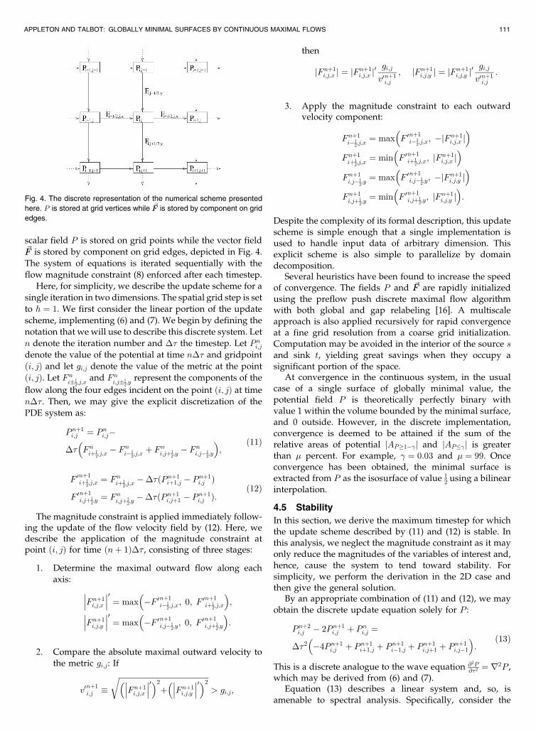
scalar field P is stored on grid points while the vector field~FF is stored by component on grid edges, depicted in Fig. 4.

The system of equations is iterated sequentially with the

flow magnitude constraint (8) enforced after each timestep.

Here, for simplicity, we describe the update scheme for a

single iteration in two dimensions. The spatial grid step is set

to h ¼ 1. We first consider the linear portion of the update

scheme, implementing (6) and (7). We begin by defining the

notation that we will use to describe this discrete system. Let

n denote the iteration number and �� the timestep. Let Pni;j

denote the value of the potential at time n�� and gridpoint

ði; jÞ and let gi;j denote the value of the metric at the point

ði; jÞ. Let Fni�1

2;j;xand Fn

i;j�12;y

represent the components of the

flow along the four edges incident on the point ði; jÞ at time

n�� . Then, we may give the explicit discretization of the

PDE system as:

Pnþ1i;j ¼ Pn

i;j�

�� Fniþ1

2;j;x� Fn

i�12;j;xþ Fn

i;jþ12;y� Fn

i;j�12;y

� �;

ð11Þ

F 0nþ1iþ1

2;j;x¼ Fn

iþ12;j;x��ðPnþ1

iþ1;j � Pnþ1i;j Þ

F 0nþ1i;jþ1

2;y¼ Fn

i;jþ12;y��ðPnþ1

i;jþ1 � Pnþ1i;j Þ:

ð12Þ

The magnitude constraint is applied immediately follow-ing the update of the flow velocity field by (12). Here, wedescribe the application of the magnitude constraint atpoint ði; jÞ for time ðnþ 1Þ�� , consisting of three stages:

1. Determine the maximal outward flow along each

axis:

Fnþ1i;j;x

�� 0 ¼ max �F 0nþ1i�1

2;j;x; 0; F 0

nþ1iþ1

2;j;x

� �;

Fnþ1i;j;y

�� 0 ¼ max �F 0nþ1i;j�1

2;y; 0; F 0

nþ1i;jþ1

2;y

� �:

2. Compare the absolute maximal outward velocity to

the metric gi;j: If

v0nþ1i;j �

ffiffiffiffiffiffiffiffiffiffiffiffiffiffiffiffiffiffiffiffiffiffiffiffiffiffiffiffiffiffiffiffiffiffiffiffiffiffiffiffiffiffiffiffiffiffiffiffiFnþ1i;j;x

�� 0� �2

þ Fnþ1i;j;y

�� 0� �2r

> gi;j;

then

jFnþ1i;j;x j ¼ jFnþ1

i;j;x j0 gi;j

v0nþ1i;j

; jFnþ1i;j;y j ¼ jFnþ1

i;j;y j0 gi;j

v0nþ1i;j

:

3. Apply the magnitude constraint to each outwardvelocity component:

Fnþ1i�1

2;j;x¼ max F 0

nþ1i�1

2;j;x; �jFnþ1

i;j;x j� �

Fnþ1iþ1

2;j;x¼ min F 0

nþ1iþ1

2;j;x; jFnþ1

i;j;x j� �

Fnþ1i;j�1

2;y¼ max F 0

nþ1i;j�1

2;y; �jFnþ1

i;j;y j� �

Fnþ1i;jþ1

2;y¼ min F 0

nþ1i;jþ1

2;y; jFnþ1

i;j;y j� �

:

Despite the complexity of its formal description, this updatescheme is simple enough that a single implementation isused to handle input data of arbitrary dimension. Thisexplicit scheme is also simple to parallelize by domaindecomposition.

Several heuristics have been found to increase the speedof convergence. The fields P and ~FF are rapidly initializedusing the preflow push discrete maximal flow algorithmwith both global and gap relabeling [16]. A multiscaleapproach is also applied recursively for rapid convergenceat a fine grid resolution from a coarse grid initialization.Computation may be avoided in the interior of the source sand sink t, yielding great savings when they occupy asignificant portion of the space.

At convergence in the continuous system, in the usualcase of a single surface of globally minimal value, thepotential field P is theoretically perfectly binary withvalue 1 within the volume bounded by the minimal surface,and 0 outside. However, in the discrete implementation,convergence is deemed to be attained if the sum of therelative areas of potential jAP�1�j and jAPj is greaterthan percent. For example, ¼ 0:03 and ¼ 99. Onceconvergence has been obtained, the minimal surface isextracted from P as the isosurface of value 1

2 using a bilinearinterpolation.

4.5 Stability

In this section, we derive the maximum timestep for whichthe update scheme described by (11) and (12) is stable. Inthis analysis, we neglect the magnitude constraint as it mayonly reduce the magnitudes of the variables of interest and,hence, cause the system to tend toward stability. Forsimplicity, we perform the derivation in the 2D case andthen give the general solution.

By an appropriate combination of (11) and (12), we mayobtain the discrete update equation solely for P :

Pnþ2i;j � 2Pnþ1

i;j þ Pni;j ¼

��2 �4Pnþ1i;j þ Pnþ1

iþ1;j þ Pnþ1i�1;j þ Pnþ1

i;jþ1 þ Pnþ1i;j�1

� �:

ð13Þ

This is a discrete analogue to the wave equation @2P@�2 ¼ r2P ,

which may be derived from (6) and (7).Equation (13) describes a linear system and, so, is

amenable to spectral analysis. Specifically, consider the


Fig. 4. The discrete representation of the numerical scheme presented

here. P is stored at grid vertices while ~FF is stored by component on grid

edges.

Z-transform over zx; zy; z� 2 CC with jzxj ¼ jzyj ¼ 1 for abounded field P :

P ðzx; zy; z� Þ ¼Xi;j;n

Pni;jz

ixz

jyzn� : ð14Þ

For P 6¼ 0, substitution into (13) gives

z2� � 2z� þ 1 ¼ ��2 �4þ zx þ z�1

x þ zy þ z�1y

� �: ð15Þ

For a stable and causal system, we require jz� j < 1. Now,the right side of (15) takes values in the range ½�8ð��Þ2; 0�over the entire spatial spectrum. The left side has rangeð�4; 0�. Therefore, in order that this equation have asolution for all spatial frequency components, we requirethat it have a solution when the right side equals �8ð��Þ2,so �� < 1ffiffi

2p . More generally, when the update is performed

in N dimensions, it is simple to show that �� < 1ffiffiffiNp as

before. The same argument may be applied to theevolution of ~FF but is not pursued here for reasons ofspace. This condition on the time step is thereforenecessary and sufficient to obtain a stable discreteimplementation.

5 METRIC WEIGHTING FUNCTIONS

Minimal surface methods have an inherent bias in favor ofsmall surfaces. In many applications, this is undesirable,resulting in incorrect or even trivial solutions. In thissection, we present a technique to automatically removethis bias.

5.1 Construction

Consider a metric that is uniformly constant throughout thedomain, g ¼ 1. This metric conveys no preference for anyparticular point through which the partition surface shouldpass. Intuitively, then, every point in the domain shouldbelong to some (globally) minimal surface. Unfortunately,as the minimal surface problem is posed, this is not the case.In order to improve the behavior of the solutions to thisproblem, then, we replace the metric g by g0 ¼ gw,introducing an appropriate weighting function w. Thisweighting function will account for the geometry of thesources and sinks, so that the minimal surface depends onlyon the data as represented by g.

Appleton and Talbot [23] considered the special case of asingle point source p in a planar image. Here, it wasdemonstrated that the introduction of the weighting function

wðxÞ ¼ 1jx�pj resulted in a continuum of minimal surfaces,

the set of all circles centered on p. In N dimensions, it is

simple to see that the modified weighting function wðxÞ ¼1

jx�pjN�1 will behave similarly, ensuring that each point in

the domain belongs to a minimal surface (a hypersphere

centered on p). These weighting functions may be extended

to other seed geometries. For a line source in three dim-

ensions, we obtain the weighting function wðxÞ ¼ 1jx�pj ,

where p is the nearest point to x on the line. More generally,

for a set of seeds which form an M-dimensional manifold

embedded in N dimensions, we should expect a weighting

function that decays as 1jx�pjN�M�1 in the neighborhood of the

manifold.

We wish to derive an unbiased flow ~FF from which we

may define the weighting function w ¼ k~FFk. This flow will

be produced by the source set s and absorbed by the sink

set t,

r � ~FF ¼ �; ð16Þ

where � is a distribution that is zero in the interior of the

domain, positive on the source set s and negative on the

sink set t, with total source weightRs �dV ¼ 1 and sink

weightRt �dV ¼ �1. There will naturally be many such

flows; here, we select a flow to minimize a measure of the

weighting function

E½w� ¼ZV

1

2w2dV ¼

ZV

1

2k~FFk2dV :

In this way, we will ensure that the weighting function is

not arbitrarily large at any particular point in space, as it

could be, for example, for some flows with large rotational

components.

We may minimize the measureE½~FF � � E½w� by variational

calculus: Consider adding a minimization parameter � to

obtainw � wðx; �Þ. Then, we may compute the first variation

with respect to � to determine the local minima of E½~FF �:

�E½~FF ��

¼ZV

~FF� � ~FFdV ¼ 0:

Here, we have set the first variation to 0 to obtain a local

minimum condition on E½w�. This minimization must be

carried out subject to the incompressibility constraint

expressed in (16). Taking the time derivative of the

constraint, we obtain the equivalent constraint r � ~FF� ¼ 0.

Therefore, ~FF� may be decomposed into cyclic components,

and ~FF is a local minimum of E½~FF � if it is locally minimal

with respect to all cyclic flows. Consider, then, ~FF� ¼ ~TTC , the

unit tangent vector over the tube formed from the set of all

points within a vanishing radius r of the smooth closed

curve C, with ~FF� ¼ 0 elsewhere. For ~FF a local minimum of

E½~FF �, we have

�E½~FF ��

¼ZV

~FF� � ~FFdV

¼ AN�1ðrÞIC

~FF� � ~TTCdC;

whereAN�1ðrÞ is the volume of theN � 1 dimensional sphere

of radius r. So, for �E½~FF �� ¼ 0, we find that the vector field is a

potential flow. Set ~FF� ¼ r�� , then, and replace the divergence

of the flow ~FF in (16) by the Laplacian of � to obtainr2� ¼ �.

We choose boundary conditions limjxj!1 r�ðxÞ ¼ 0 so that

the flow is zero at infinity. � is then determined up to the

addition of a constant which will not affect the weighting

function w ¼ jr�j.Observe, now, that all isosurfaces S of � in the interior of

the domain have constant net fluxHS r� � ~NNSdS ¼ 1. As

w ¼ jr�j, we then obtainHS wdS ¼ 1 over all isosurfaces of

�, withHS wdS � 1 for all closed surfaces S containing the

seeds. So, the isosurfaces of � form the set of minimal


surfaces under the metric w. In general, we have r� 6¼ 0almost everywhere; therefore, almost every point in thedomain belongs to some minimal weighted surface underthe metric w as desired.

5.2 Implementation

For the regular grids considered in this paper, the

weighting functions may be computed by convolving the

distribution � with the Green’s function � with the

property r2� ¼ �ðxÞ. In IR2, this is � ¼ 12 lnðjxjÞ, while,

in IR3, this is � ¼ � 14 jxj [29]. This convolution may be

efficiently computed on discrete images using the Fast

Fourier Transform. The gradient of � may then be

numerically estimated in the discrete grid to obtain the

weighting function w.

Fig. 5 shows an example of a set of seed points and the

process of computing an appropriate weighting function.

The weighting function is highest in the neighborhood of

point sources and at the endpoints of line sources.

Fig. 6 depicts the application of metric weighting in the

segmentation of a microscope image of a protist, Chilomonas

Paramecium. Presented are segmentations using a simple

seed geometry and a complex seed geometry. The metric

weighting scheme proposed in this section produces similar

results on the two examples, demonstrating that it does not

significantly bias the segmentation.

6 RESULTS

In this section, we demonstrate the results of using globallyminimal surfaces for 2D and 3D medical image segmenta-tion and for stereo matching. All results were obtainedusing the metric weighting scheme introduced in Section 5,except where otherwise noted. Timings were obtained on aquad 2.2GHz AMD Opteron Processor 848 under the Linuxoperating system. The algorithm presented here has beenimplemented in C with no assembly optimizations. Timingsfor minimum cuts have been obtained using the BoostGraph Library implementation of the preflow-push algo-rithm [30]. The preflow-push algorithm is generallyaccepted as a fast general-purpose maximum flow algo-rithm, although a faster image-specific maximum flowalgorithm presented in [31] has not been considered here.

6.1 Two-Dimensional Image Segmentation

Object boundaries are often difficult to detect alongtransitions to adjacent objects with similar features. Seg-mentation via minimal contours uses the regularization ofthe segmentation contour to avoid leaking across such gaps.The authors have previously developed an algorithm,Globally Optimal Geodesic Active Contours (GOGAC)[23], which efficiently computes globally minimal contoursin planar Riemannian spaces using the planar duality inSection 3.4. Here, we apply discrete minimal cuts, GOGAC,and the algorithm presented in this paper to segment a


Fig. 5. Metric weighting example. (a) The seed geometry. Source points are depicted, while the sink points are the image boundary. (b) The function� computed by convolution. (c) The metric weighting w computed from the numerical derivative of �.

Fig. 6. An example of the application of metric weighting. (a) A microscope image of a protist, Chilomonas Paramecium. (b) Segmentation using asingle internal seed. (c) Segmentation with complex seed geometry.

microscope image of a cluster of cells (Fig. 7a) and comparethe results. In spite of its apparent simplicity, this problemdemonstrates the challenge of delineating faint boundariesbetween cells without leaking.

We compute a metric (Fig. 7b) from the microscopeimage as described in (2), with default parameters: p ¼ 1," ¼ 0, and � ¼ 1. Low metric regions are dark, while highmetric regions are bright. The regions of low metriccorrespond to the boundaries of the cells, except wherethe cells overlap. The metric has been weighted accordingto the method described in Section 5 (not displayed).

The segmentation of each cell is performed indepen-dently in sequence for each method. The source sets aredepicted in Figs. 7b, 7c, and 7d, while the sink is the imageboundary. The discrete minimal cut produces a clear gridbias and a poor segmentation. GOGAC and the continuousmaximal flow algorithm solve the same continuous optimi-zation problem and are in close agreement. Note that the

continuous segmentations follow the perceived cell con-tours despite the weakness of local cues.

The image depicted in Fig. 7a has dimensions 231� 221.We reduce the amount of computation required byexpanding the sink to include only the cells of interest, a

region of size 150� 100.The discrete minimal cuts required 0:41 seconds to

compute in total. GOGAC required 0:73 seconds to computein total. The continuous minimal surface algorithm pre-sented here required 0:68 seconds in total to converge.

6.2 Three-Dimensional Image Segmentation

Here, we demonstrate the application of globally minimalsurfaces to a 3D segmentation problem. Fig. 8 depicts aComputed Tomography scan of a chest in which thetwo lungs are segmented. We compare the results fromthe application of globally minimal surfaces to thoseobtained using geodesic active surfaces and discrete


Fig. 7. Segmentation of a cluster of cells in a microscope image. (a) The original image. (b) Discrete minimal cuts. (c) Globally Optimal Geodesic

Active Contours. (d) Globally minimal surfaces.

minimal cuts. The minimal cut and minimal surfacesegmentations use the same input, i.e., the same weightedmetric, as well as the seeds. The sources are ellipsoidsinside each lung, while the sinks are the five volumeboundaries not including the uppermost face where thelung is open. The geodesic active surfaces are unable to usethe weighted metric due to the large range of metric valuesproduced. Instead, they use the unweighted metric and areinitialized from large ellipsoids inside each lung. Anadditional artificial inflation term was also used to drivethe level sets to fill the lungs. The two lungs are segmentedindependently in all three methods.

The top row of Fig. 8 depicts corresponding 2D slices ofthe original CT data, the metric derived from this data, andthe weighted metric for the right lung. The weighted metrichas been displayed on a logarithmic scale due to its largerange of values. The middle row of Fig. 8 shows correspond-ing 2D slices of segmentations by each of the methodsconsidered here: geodesic active surfaces, minimal cuts, andglobally minimal surfaces. The bottom row of Fig. 8 provides3D views of the sources as well as the segmentationsobtained by the different methods.

The geodesic active surfaces produce a poor segmentation.At the top of the lung, the inflation term is too strong, causingthe surface to leak through the weak edges of the lung.Elsewhere, the surface has failed to completely fill the lung.This behavior is common in the application of active contourmethods and, as in this case, sometimes hard to avoid.

The discrete minimal cuts also produce inaccuratesegmentations. Observe the bias toward the grid directions,which can be clearly seen as the flat boundaries in the

interior surfaces at the top of the lungs. By contrast, thecontinuous minimal surface does not exhibit such direc-tional bias, giving a faithful segmentation.

The CT data shown in Fig. 8 has dimensions200� 160� 90. The Geodesic Active Surfaces required

279 seconds to converge to the final result. The discreteminimal cuts required 44 seconds to compute using thepreflow push algorithm. The continuous minimal surfacealgorithm required only 28:8 seconds using three scales.

The minimal surface algorithm uses a multiscale frame-work to obtain a fast initialization from the solution at acoarser scale. The fields P and ~FF are initialized using aminimum cut at the coarsest scales. In this example, the

minimal surface segmentation is faster than the mini-mum cut segmentation due to the multiscale framework.

6.3 Three-Dimensional Scene Reconstruction fromStereo Images

The reconstruction of a 3D scene from two or more images

is often performed using an energy minimization approach[13], [14]. Here, we adapt the framework of [14], replacingtheir discrete graph cut by a globally minimal surface.

In stereo matching, a number of metrics have beenproposed for real and synthetic images. Here, we use the

zero-mean normalized cross correlation (ZNCC) window-based matching score, which performs well on natural sceneswith lighting variation and specular reflections and may becomputed very efficiently [12]. We set g ¼ 1� ZNCC to

convert high matching scores to low metrics suitable forminimization. Matching scores are computed using a


Fig. 8. Segmentation of the lungs in a CT image of a chest. Top row: 2D slices of original data, metric, and weighted metric (log scale). Middle row:

2D slices of segmentations by geodesic active surfaces, minimal cuts, and globally minimal surfaces. Bottom row: 3D views of seeds and

segmentations by geodesic active surfaces, minimal cuts, and globally minimal surfaces.

5� 5 window. The stereo pair being analyzed has a disparityrange of ½�15; 0�. Following [14], the source and sink areconnected to the first and last layers of the disparity volume.Both the discrete minimal cut and the globally minimalsurface are computed from the same metric.

The results of the stereo matching are depicted in Fig. 9.These results are shown as disparity maps (depth maps) aswell as surface meshes. We observe that the discreteminimal cut produces large flat regions due to the smallnumber of disparities and, hence, poor depth resolution ofdiscrete methods. Compared to the graph cut, we can see agreat deal more detail in the disparity map computed by theglobally minimal surface. This includes the surface textureof the bushes as well as the third parking meter. In additionto the improvement in depth resolution is the rotationalinvariance of the continuous method. This can be seen onthe frame of the car, where the discrete method produces a“rectangular” curve, while the minimal surface produces astraight line.

The stereo image pair used here has dimensions 256� 240.The discrete minimal cut required 11:3 seconds to compute.The continuous minimal surface algorithm required only8:3 seconds.

6.4 Accuracy

In the continuous theory, the system of PDEs presentedin (6), (7), and (8) was proven to obtain the globallyminimal surface at convergence. However, in order todevelop a practical algorithm, it was necessary todiscretize these equations. An explicit, first-order finite

difference discretization was presented in Section 4.4. It isnatural to question whether this discretization introducesgrid bias into the solution surfaces.

To address this question, we compare the surfaceobtained by the proposed discretization with the analyticsolution on a simple problem in three dimensions, thecomputation of a catenoid. Consider two circles of equalradius R0 whose centers lie along the z-axis. These circles liein the planes z ¼ �H and z ¼ H, respectively. The minimalsurface which connects these two circles is a catenoid. Anillustration of such a nontrivial minimal surface is some-times given using soap bubbles. The surface points of thiscatenoid ðx; y; zÞ are described by:

x ¼ R0 coshz

R0

� �cosð�Þ;

y ¼ R0 coshz

R0

� �sinð�Þ;

where � 2 ½0; 2 Þ and z 2 ½�H;H�. Here, R0 is selected tomeet the boundary condition R0 cosh H

R0

� ¼ R.

We set R ¼ 35 and H ¼ 15 and compare the analytic andnumeric solutions. The algorithm proposed in this paper isdiscretized on a 120� 120� 31 grid with grid step h ¼ 1. Forthe Euclidean metric, we set g ¼ 1 everywhere, withoutmetric weighting. For this problem, we may enforce thecircular boundary conditions by placing disk-shapedsources of radius R on the vertical boundaries z ¼ H andz ¼ �H, and sinks elsewhere on the volume boundary. Theresults for this comparison are presented in Fig. 10. Fig. 10adepicts the analytic solution. Figs. 10b and 10c depict the


Fig. 9. Stereo matching from two views. (a) and (b) The original images. (c) Disparity map obtained by a discrete maximal flow. (d) Disparity map

obtained by a globally minimal surface. Note the improved detail.

numeric solution obtained from P , respectively, by thresh-

olding and by isosurface extraction. The isosurface and the

analytic solution are in clear agreement. By contrast, the

threshold result demonstrates that it is important to extract

isosurfaces in order to avoid discretisation artifacts. This

result is also the best that a discrete method such as a graph

cut could obtain without increasing the grid resolution.

Fig. 10d depicts a horizontal slice z ¼ 0 through the potential

function P computed by the new algorithm, overlayed with

the corresponding cross-section of the analytic solution (a

circle of radius R0). Fig. 10e depicts a vertical slice x ¼ 0

through P , overlayed with the corresponding cross-section

of the analytic solution (two catenaries). In both Figs. 10c

and 10d, the analytic solution closely coincides with the

isosurface P ¼ 12 .

In order to make a quantitative comparison, we

measured the average distance between the analytic surface

and the computed isosurface. The mean distance between

these surfaces was 0:09 while the root-mean-square distance

was 0:11. In this simple example then, the new algorithm

obtains a result which is accurate to approximately

10 percent of the grid step.

7 CONCLUSIONS

In this paper, we have developed a new algorithm to

compute globally minimal weighted surfaces for image

segmentation and stereo matching.

We obtain these surfaces using a nonlinear system of

partial differential equations which simulate an ideal fluid

flow. The velocity of the flow is constrained in magnitude by

a spatially varying metric, itself derived from the image or

images being analyzed. This simulation is performed using

a simple finite difference scheme with explicit update step.

To improve efficiency, a multiresolution scheme is used to

reduce computational costs and the solution is approxi-

mated at the coarsest scale by a discrete maximal flow.A proof is given that, at convergence, the algorithm

produces a globally maximal flow. The minimal surface is

simply an isosurface of the auxiliary potential function. A

proof that the system converges is left to future work.Results are given demonstrating the application of

globally minimal surfaces to 2D and 3D segmentation and

to stereo matching. Comparison to an existing optimal

geodesic active contour for 2D images demonstrates close

similarity. Comparisons for 3D segmentation and stereo

matching demonstrate that globally minimal surfaces over-

come the existing problems with graph-based approaches

and with active contours. On a simple test problem with

known analytic solution, the discrete implementation of this

algorithm was shown to be accurate to 10 percent of the

grid step size. The algorithm is also efficient when

compared to previous methods. These results suggest that

many existing applications using geodesic active surfaces or

graph cuts will benefit from the improved accuracy and

reliability of globally minimal surfaces.


Fig. 10. The catenoid test problem. (a) The correct minimal surface, constructed analytically. (b) The discrete minimal surface obtained bythresholding P 0:5. (c) The minimal surface obtained as the isosurface P ¼ 1

2 . (d) A horizontal slice through P . The correct cross-section isoverlayed in black. (e) A vertical slice through P . The correct cross-section is overlayed in black.

ACKNOWLEDGMENTS

This work was carried out when B. Appleton was affiliated

with the School of ITEE, The Univerity of Queensland, QLD

4067, Australia, and H. Talbot was affiliated with CSIRO,

Mathematics and Information Sciences, Sydney, Australia.

The authors would like to acknowledge Simon Long of the

University of Queensland for an interesting discussion

leading to the numerical implementation of the metric

weighting scheme presented in this paper. We would also

like to thank Rob Dunne of CSIRO Mathematical and

Information Sciences for the use of his computer to obtain

the results in Section 6.

REFERENCES

[1] M. Kass, A. Witkin, and D. Terzopoulos, “Snakes: ActiveContour Models,” Int’l J. Computer Vision, vol. 1, no. 4, pp. 321-331, 1998.

[2] S. Osher and J.A. Sethian, “Fronts Propagating with Curvature-Dependent Speed: Algorithms Based on Hamilton-Jacobi For-mulations,” J. Computational Physics, vol. 79, pp. 12-49, 1988,citeseer.nj.nec.com/osher88fronts.html.

[3] J.A. Sethian, Level Set Methods and Fast Marching Methods—EvolvingInterfaces in Computational Geometry, Fluid Mechanics, ComputerVision, and Materials Science. Cambridge Univ. Press, 1999.

[4] V. Caselles, R. Kimmel, and G. Sapiro, “Geodesic ActiveContours,” Int’l J. Computer Vision, vol. 22, no. 1, pp. 61-79, 1997.

[5] V. Caselles, R. Kimmel, G. Sapiro, and C. Sbert, “Minimal SurfacesBased Object Segmentation,” IEEE Trans. Pattern Analysis andMachine Intelligence, vol. 19, pp. 394-398, 1997.

[6] E. Dijkstra, “A Note on Two Problems in Connexion withGraphs,” Numerische Mathematik, vol. 1, pp. 269-271, 1959.

[7] J.L.R. Ford and D.R. Fulkerson, Flows in Networks. Princeton, N.J.:Princeton Univ. Press, 1962.

[8] L.D. Cohen, “On Active Contour Models and Balloons,” ComputerVision, Graphics, and Image Processing. Image Understanding, vol. 53,no. 2, pp. 211-218, 1991, citeseer.nj.nec.com/cohen91active.html.

[9] C. Xu and J.L. Prince, “Snakes, Shapes and Gradient VectorFlow,” IEEE Trans. Image Processing, vol. 7, no. 3, pp. 359-369,Mar. 1998.

[10] S. Lloyd, “Stereo Matching Using Intra- and Inter-Row DynamicProgramming,” Pattern Recognition Letters, vol. 4, pp. 273-277,Sept. 1986.

[11] Y. Ohta and T. Kanade, “Stereo by Intra- and Inter-Scanline SearchUsing Dynamic Programming,” IEEE Trans. Pattern AnalysisMachine Intelligence, vol. 7, no. 2, pp. 139-154, Mar. 1985.

[12] C. Sun, “Fast Stereo Matching Using Rectangular Subregioningand 3D Maximum-Surface Techniques,” Int’l J. Computer Vision,vol. 47, nos. 1/2/3, pp. 99-117, May 2002.

[13] C. Leung, B. Appleton, and C. Sun, “Fast Stereo Matching byIterated Dynamic Programming and Quadtree Subregioning,”Proc. British Machine Vision Conf., S.B.A. Hoppe and T. Ellis, eds.,vol. 1, pp. 97-106, Sept. 2004.

[14] S. Roy and I.J. Cox, “A Maximum-Flow Formulation of the n-Camera Stereo Correspondence Problem,” Proc. Int’l Conf.Computer Vision, pp. 492-499, Jan. 1998.

[15] P. Bamford and B. Lovell, “Unsupervised Cell Nucleus Segmenta-tion with Active Contours,” Signal Processing, special issue ondeformable models and techniques for image and signal proces-sing, vol. 71, no. 2, pp. 203-213, 1998.

[16] R. Sedgewick, Algorithms in C, third ed. Addison-Wesley, 2002.[17] J.N. Tsitsiklis, “Efficient Algorithms for Globally Optimal Trajec-

tories,” IEEE Trans. Automatic Control, vol. 40, no. 9, pp. 1528-1538,Sept. 1995.

[18] J. Sethian, “A Fast Marching Level Set Method for MonotonicallyAdvancing Fronts,” Proc. Nat’l Academy of Sciences, vol. 93, no. 4,pp. 1591-1595, 1996, citeseer.nj.nec.com/sethian95fast.html.

[19] T.C. Hu, Integer Programming and Network Flows. Reading, Mass.:Addison-Wesley, 1969.

[20] Y. Boykov and V. Kolmogorov, “Computing Geodesics andMinimal Surfaces via Graph Cuts,” Proc. Int’l Conf. ComputerVision, pp. 26-33, Oct. 2003.

[21] R. Goldenberg, R. Kimmel, E. Rivlin, and M. Rudzsky, “FastGeodesic Active Contours,” IEEE Trans. Image Processing, vol. 10,no. 10, pp. 1467-1475, 2001.

[22] L.D. Cohen and R. Kimmel, “Global Minimum for Active ContourModels: A Minimal Path Approach,” Intl J. Computer Vision, vol. 24,no. 1, pp. 57-78, Aug. 1997, citeseer.nj.nec.com/cohen97global.html.

[23] B. Appleton and H. Talbot, “Globally Optimal Geodesic ActiveContours,” J. Math. Imaging and Vision, July 2005.

[24] G. Strang, “Maximal Flow through a Domain,” Math. Program-ming, vol. 26, pp. 123-143, 1983.

[25] M. Iri, Survey of Mathematical Programming. North-Holland,Amsterdam, 1979.

[26] K. Weihe, “Maximum ðs; tÞ-Flows in Planar Networks inOðjV jlogjV jÞ Time,” J. Computer and System Sciences, vol. 55, no. 3,pp. 454-475, Dec. 1997.

[27] J.S. Mitchell, “On Maximum Flows in Polyhedral Domains,” Proc.Fourth Ann. Symp. Computational Geometry, pp. 341-351, 1988.

[28] B. Appleton and H. Talbot, “Globally Optimal Surfaces byContinuous Maximal Flows,” Digital Image Computing: Techniquesand Applications, Proc. VIIth APRS Conf., vol. 2, pp. 987-996, Dec.2003.

[29] G. Strang, Introduction to Applied Mathematics. Wellesley-Cam-bridge Press, 1986.

[30] J. Siek, L.-Q. Lee, and A. Lumsdaine, The Boost Graph Library: UserGuide and Reference Manual. Addison-Wesley, 2002.

[31] Y. Boykov and V. Kolmogorov, “An Experimental Comparison ofMin-Cut/Max-Flow Algorithms for Energy Minimization inVision,” IEEE Trans. Pattern Analysis and Machine Intelligence,vol. 26, no. 9, pp. 1124-1137, Sept. 2004.

Ben Appleton completed the PhD degree in thearea of image analysis at the University ofQueensland (UQ), Australia, in 2005. He re-ceived degrees in engineering and science fromthe University of Queensland in 2001 and wasawarded a university medal. He is currently aresearch fellow in the Electromagnetics andImaging research group of UQ. He has con-tributed 17 research papers to internationaljournals and conferences and was awarded the

prize for Best Student Paper at Digital Image Computing: Techniquesand Applications (DICTA) 2003. His research interests include imagesegmentation, stereo vision, and cardiac modeling.

Hugues Talbot received the Engineering de-gree from Ecole Centrale de Paris in 1989, theDiplome d’Etudes Avancee (Masters) from theUniversite Paris VI in 1990 and the PhD degreein mathematical morphology from Ecole Natio-nale Superieure des Mines de Paris in 2003,under the guidance of professors Linn W. Hobbs(MIT), Jean Serra, and Dominique Jeulin(ENSMP). His PhD work was a collaborativework between the Isover Saint Gobain Corpora-

tion, France; MIT, Cambridge, United States; and ENSMP, France. Hehas been affiliated with CSIRO, Mathematical and Information Sciences,Sydney, Australia, since 1994 and is now an assistant professor at EcoleSuperieure d’Ingenieurs en Electronique et Electrotechnique, France.He has worked on a number of applied projects in image analysis withvarious companies and has contributed more than 50 publications tointernational journals and conferences. His research interests includeimage segmentation, linear feature analysis, texture analysis, PDEs,and algorithms.

. For more information on this or any other computing topic,please visit our Digital Library at www.computer.org/publications/dlib.


Globally minimal surfaces by continuous maximal flows

Documents

Transcript of Globally minimal surfaces by continuous maximal flows