Globalization and Cycles

Thomas J. Sargent and John Stachurski

January 13, 2022

1 Contents

• Overview 2• Key Ideas 3• Model 4• Simulation 5• Exercises 6• Solutions 7

2 Overview

In this lecture, we review the paper Globalization and Synchronization of Innovation Cyclesby Kiminori Matsuyama, Laura Gardini and Iryna Sushko.

This model helps us understand several interesting stylized facts about the world economy.

One of these is synchronized business cycles across different countries.

Most existing models that generate synchronized business cycles do so by assumption, sincethey tie output in each country to a common shock.

They also fail to explain certain features of the data, such as the fact that the degree of syn-chronization tends to increase with trade ties.

By contrast, in the model we consider in this lecture, synchronization is both endogenous andincreasing with the extent of trade integration.

In particular, as trade costs fall and international competition increases, innovation incentivesbecome aligned and countries synchronize their innovation cycles.

Let’s start with some imports:

In [1]: import numpy as npimport matplotlib.pyplot as plt%matplotlib inlineimport seaborn as snsfrom numba import jit, vectorizefrom ipywidgets import interact

1

2.1 Background

The model builds on work by Judd [3], Deneckner and Judd [1] and Helpman and Krugman[2] by developing a two-country model with trade and innovation.

On the technical side, the paper introduces the concept of coupled oscillators to economicmodeling.

As we will see, coupled oscillators arise endogenously within the model.

Below we review the model and replicate some of the results on synchronization of innovationacross countries.

3 Key Ideas

It is helpful to begin with an overview of the mechanism.

3.1 Innovation Cycles

As discussed above, two countries produce and trade with each other.

In each country, firms innovate, producing new varieties of goods and, in doing so, receivingtemporary monopoly power.

Imitators follow and, after one period of monopoly, what had previously been new varietiesnow enter competitive production.

Firms have incentives to innovate and produce new goods when the mass of varieties of goodscurrently in production is relatively low.

In addition, there are strategic complementarities in the timing of innovation.

Firms have incentives to innovate in the same period, so as to avoid competing with substi-tutes that are competitively produced.

This leads to temporal clustering in innovations in each country.

After a burst of innovation, the mass of goods currently in production increases.

However, goods also become obsolete, so that not all survive from period to period.

This mechanism generates a cycle, where the mass of varieties increases through simultaneousinnovation and then falls through obsolescence.

3.2 Synchronization

In the absence of trade, the timing of innovation cycles in each country is decoupled.

This will be the case when trade costs are prohibitively high.

If trade costs fall, then goods produced in each country penetrate each other’s markets.

As illustrated below, this leads to synchronization of business cycles across the two countries.

2

4 Model

Let’s write down the model more formally.

(The treatment is relatively terse since full details can be found in the original paper)

Time is discrete with 𝑡 = 0, 1, ….

There are two countries indexed by 𝑗 or 𝑘.

In each country, a representative household inelastically supplies 𝐿𝑗 units of labor at wagerate 𝑤𝑗,𝑡.

Without loss of generality, it is assumed that 𝐿1 ≥ 𝐿2.

Households consume a single nontradeable final good which is produced competitively.

Its production involves combining two types of tradeable intermediate inputs via

𝑌𝑘,𝑡 = 𝐶𝑘,𝑡 = (𝑋𝑜

𝑘,𝑡1 − 𝛼)

1−𝛼(𝑋𝑘,𝑡

𝛼 )𝛼

Here 𝑋𝑜𝑘,𝑡 is a homogeneous input which can be produced from labor using a linear, one-for-

one technology.

It is freely tradeable, competitively supplied, and homogeneous across countries.

By choosing the price of this good as numeraire and assuming both countries find it optimalto always produce the homogeneous good, we can set 𝑤1,𝑡 = 𝑤2,𝑡 = 1.

The good 𝑋𝑘,𝑡 is a composite, built from many differentiated goods via

𝑋1− 1𝜎

𝑘,𝑡 = ∫Ω𝑡

[𝑥𝑘,𝑡(𝜈)]1− 1𝜎 𝑑𝜈

Here 𝑥𝑘,𝑡(𝜈) is the total amount of a differentiated good 𝜈 ∈ Ω𝑡 that is produced.

The parameter 𝜎 > 1 is the direct partial elasticity of substitution between a pair of varietiesand Ω𝑡 is the set of varieties available in period 𝑡.We can split the varieties into those which are supplied competitively and those supplied mo-nopolistically; that is, Ω𝑡 = Ω𝑐

𝑡 + Ω𝑚𝑡 .

4.1 Prices

Demand for differentiated inputs is

𝑥𝑘,𝑡(𝜈) = (𝑝𝑘,𝑡(𝜈)𝑃𝑘,𝑡

)−𝜎 𝛼𝐿𝑘

𝑃𝑘,𝑡

Here

• 𝑝𝑘,𝑡(𝜈) is the price of the variety 𝜈 and• 𝑃𝑘,𝑡 is the price index for differentiated inputs in 𝑘, defined by

3

[𝑃𝑘,𝑡]1−𝜎 = ∫

Ω𝑡

[𝑝𝑘,𝑡(𝜈)]1−𝜎𝑑𝜈

The price of a variety also depends on the origin, 𝑗, and destination, 𝑘, of the goods becauseshipping varieties between countries incurs an iceberg trade cost 𝜏𝑗,𝑘.

Thus the effective price in country 𝑘 of a variety 𝜈 produced in country 𝑗 becomes 𝑝𝑘,𝑡(𝜈) =𝜏𝑗,𝑘 𝑝𝑗,𝑡(𝜈).Using these expressions, we can derive the total demand for each variety, which is

𝐷𝑗,𝑡(𝜈) = ∑𝑘

𝜏𝑗,𝑘𝑥𝑘,𝑡(𝜈) = 𝛼𝐴𝑗,𝑡(𝑝𝑗,𝑡(𝜈))−𝜎

where

𝐴𝑗,𝑡 ∶= ∑𝑘

𝜌𝑗,𝑘𝐿𝑘(𝑃𝑘,𝑡)1−𝜎 and 𝜌𝑗,𝑘 = (𝜏𝑗,𝑘)1−𝜎 ≤ 1

It is assumed that 𝜏1,1 = 𝜏2,2 = 1 and 𝜏1,2 = 𝜏2,1 = 𝜏 for some 𝜏 > 1, so that

𝜌1,2 = 𝜌2,1 = 𝜌 ∶= 𝜏1−𝜎 < 1

The value 𝜌 ∈ [0, 1) is a proxy for the degree of globalization.

Producing one unit of each differentiated variety requires 𝜓 units of labor, so the marginalcost is equal to 𝜓 for 𝜈 ∈ Ω𝑗,𝑡.

Additionally, all competitive varieties will have the same price (because of equal marginalcost), which means that, for all 𝜈 ∈ Ω𝑐,

𝑝𝑗,𝑡(𝜈) = 𝑝𝑐𝑗,𝑡 ∶= 𝜓 and 𝐷𝑗,𝑡 = 𝑦𝑐

𝑗,𝑡 ∶= 𝛼𝐴𝑗,𝑡(𝑝𝑐𝑗,𝑡)−𝜎

Monopolists will have the same marked-up price, so, for all 𝜈 ∈ Ω𝑚 ,

𝑝𝑗,𝑡(𝜈) = 𝑝𝑚𝑗,𝑡 ∶= 𝜓

1 − 1𝜎

and 𝐷𝑗,𝑡 = 𝑦𝑚𝑗,𝑡 ∶= 𝛼𝐴𝑗,𝑡(𝑝𝑚

𝑗,𝑡)−𝜎

Define

𝜃 ∶= 𝑝𝑐𝑗,𝑡

𝑝𝑚𝑗,𝑡

𝑦𝑐𝑗,𝑡

𝑦𝑚𝑗,𝑡

= (1 − 1𝜎)

1−𝜎

Using the preceding definitions and some algebra, the price indices can now be rewritten as

(𝑃𝑘,𝑡𝜓 )

1−𝜎= 𝑀𝑘,𝑡 + 𝜌𝑀𝑗,𝑡 where 𝑀𝑗,𝑡 ∶= 𝑁𝑐

𝑗,𝑡 + 𝑁𝑚𝑗,𝑡𝜃

The symbols 𝑁𝑐𝑗,𝑡 and 𝑁𝑚

𝑗,𝑡 will denote the measures of Ω𝑐 and Ω𝑚 respectively.

4

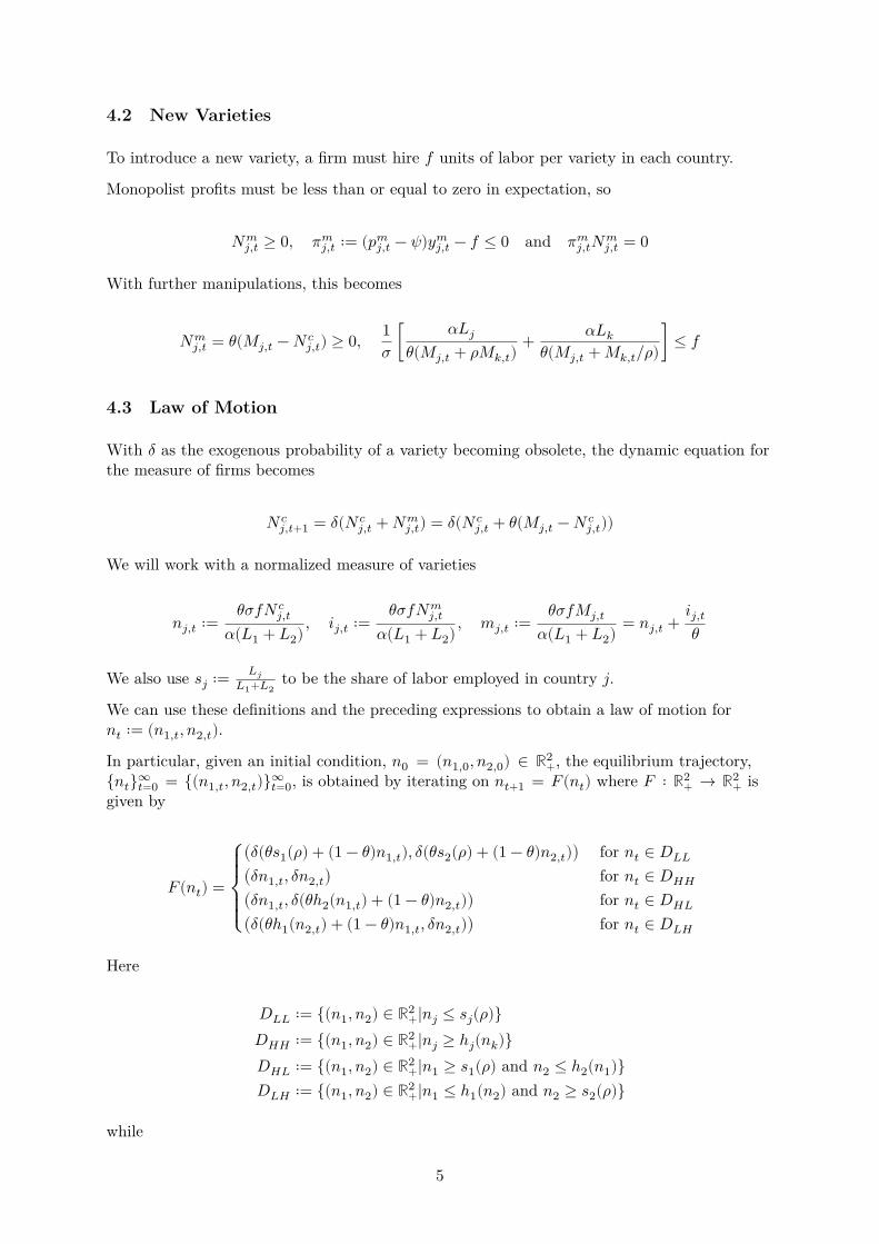
4.2 New Varieties

To introduce a new variety, a firm must hire 𝑓 units of labor per variety in each country.

Monopolist profits must be less than or equal to zero in expectation, so

𝑁𝑚𝑗,𝑡 ≥ 0, 𝜋𝑚

𝑗,𝑡 ∶= (𝑝𝑚𝑗,𝑡 − 𝜓)𝑦𝑚

𝑗,𝑡 − 𝑓 ≤ 0 and 𝜋𝑚𝑗,𝑡𝑁𝑚

𝑗,𝑡 = 0

With further manipulations, this becomes

𝑁𝑚𝑗,𝑡 = 𝜃(𝑀𝑗,𝑡 − 𝑁𝑐

𝑗,𝑡) ≥ 0, 1𝜎 [ 𝛼𝐿𝑗

𝜃(𝑀𝑗,𝑡 + 𝜌𝑀𝑘,𝑡)+ 𝛼𝐿𝑘

𝜃(𝑀𝑗,𝑡 + 𝑀𝑘,𝑡/𝜌)] ≤ 𝑓

4.3 Law of Motion

With 𝛿 as the exogenous probability of a variety becoming obsolete, the dynamic equation forthe measure of firms becomes

𝑁𝑐𝑗,𝑡+1 = 𝛿(𝑁𝑐

𝑗,𝑡 + 𝑁𝑚𝑗,𝑡) = 𝛿(𝑁𝑐

𝑗,𝑡 + 𝜃(𝑀𝑗,𝑡 − 𝑁𝑐𝑗,𝑡))

We will work with a normalized measure of varieties

𝑛𝑗,𝑡 ∶= 𝜃𝜎𝑓𝑁𝑐𝑗,𝑡

𝛼(𝐿1 + 𝐿2) , 𝑖𝑗,𝑡 ∶= 𝜃𝜎𝑓𝑁𝑚𝑗,𝑡

𝛼(𝐿1 + 𝐿2) , 𝑚𝑗,𝑡 ∶= 𝜃𝜎𝑓𝑀𝑗,𝑡𝛼(𝐿1 + 𝐿2) = 𝑛𝑗,𝑡 + 𝑖𝑗,𝑡

𝜃

We also use 𝑠𝑗 ∶= 𝐿𝑗𝐿1+𝐿2

to be the share of labor employed in country 𝑗.

We can use these definitions and the preceding expressions to obtain a law of motion for𝑛𝑡 ∶= (𝑛1,𝑡, 𝑛2,𝑡).In particular, given an initial condition, 𝑛0 = (𝑛1,0, 𝑛2,0) ∈ ℝ2

+, the equilibrium trajectory,𝑛𝑡∞

𝑡=0 = (𝑛1,𝑡, 𝑛2,𝑡)∞𝑡=0, is obtained by iterating on 𝑛𝑡+1 = 𝐹(𝑛𝑡) where 𝐹 ∶ ℝ2

+ → ℝ2+ is

given by

𝐹(𝑛𝑡) =

⎧⎨⎩

(𝛿(𝜃𝑠1(𝜌) + (1 − 𝜃)𝑛1,𝑡), 𝛿(𝜃𝑠2(𝜌) + (1 − 𝜃)𝑛2,𝑡)) for 𝑛𝑡 ∈ 𝐷𝐿𝐿(𝛿𝑛1,𝑡, 𝛿𝑛2,𝑡) for 𝑛𝑡 ∈ 𝐷𝐻𝐻(𝛿𝑛1,𝑡, 𝛿(𝜃ℎ2(𝑛1,𝑡) + (1 − 𝜃)𝑛2,𝑡)) for 𝑛𝑡 ∈ 𝐷𝐻𝐿(𝛿(𝜃ℎ1(𝑛2,𝑡) + (1 − 𝜃)𝑛1,𝑡, 𝛿𝑛2,𝑡)) for 𝑛𝑡 ∈ 𝐷𝐿𝐻

Here

𝐷𝐿𝐿 ∶= (𝑛1, 𝑛2) ∈ ℝ2+|𝑛𝑗 ≤ 𝑠𝑗(𝜌)

𝐷𝐻𝐻 ∶= (𝑛1, 𝑛2) ∈ ℝ2+|𝑛𝑗 ≥ ℎ𝑗(𝑛𝑘)

𝐷𝐻𝐿 ∶= (𝑛1, 𝑛2) ∈ ℝ2+|𝑛1 ≥ 𝑠1(𝜌) and 𝑛2 ≤ ℎ2(𝑛1)

𝐷𝐿𝐻 ∶= (𝑛1, 𝑛2) ∈ ℝ2+|𝑛1 ≤ ℎ1(𝑛2) and 𝑛2 ≥ 𝑠2(𝜌)

while

5

𝑠1(𝜌) = 1 − 𝑠2(𝜌) = min 𝑠1 − 𝜌𝑠21 − 𝜌 , 1

and ℎ𝑗(𝑛𝑘) is defined implicitly by the equation

1 = 𝑠𝑗ℎ𝑗(𝑛𝑘) + 𝜌𝑛𝑘

+ 𝑠𝑘ℎ𝑗(𝑛𝑘) + 𝑛𝑘/𝜌

Rewriting the equation above gives us a quadratic equation in terms of ℎ𝑗(𝑛𝑘).Since we know ℎ𝑗(𝑛𝑘) > 0 then we can just solve the quadratic equation and return the posi-tive root.

This gives us

ℎ𝑗(𝑛𝑘)2 + ((𝜌 + 1𝜌)𝑛𝑘 − 𝑠𝑗 − 𝑠𝑘) ℎ𝑗(𝑛𝑘) + (𝑛2

𝑘 − 𝑠𝑗𝑛𝑘𝜌 − 𝑠𝑘𝑛𝑘𝜌) = 0

5 Simulation

Let’s try simulating some of these trajectories.

We will focus in particular on whether or not innovation cycles synchronize across the twocountries.

As we will see, this depends on initial conditions.

For some parameterizations, synchronization will occur for “most” initial conditions, while forothers synchronization will be rare.

The computational burden of testing synchronization across many initial conditions is nottrivial.

In order to make our code fast, we will use just in time compiled functions that will get calledand handled by our class.

These are the @jit statements that you see below (review this lecture if you don’t recall howto use JIT compilation).

Here’s the main body of code

In [2]: @jit(nopython=True)def _hj(j, nk, s1, s2, θ, δ, ρ):

"""If we expand the implicit function for h_j(n_k) then we find thatit is quadratic. We know that h_j(n_k) > 0 so we can get itsvalue by using the quadratic form"""# Find out who's h we are evaluatingif j == 1:

sj = s1sk = s2

else:sj = s2sk = s1

6

# Coefficients on the quadratic a x^2 + b x + c = 0a = 1.0b = ((ρ + 1 / ρ) * nk - sj - sk)c = (nk * nk - (sj * nk) / ρ - sk * ρ * nk)

# Positive solution of quadratic formroot = (-b + np.sqrt(b * b - 4 * a * c)) / (2 * a)

return root

@jit(nopython=True)def DLL(n1, n2, s1_ρ, s2_ρ, s1, s2, θ, δ, ρ):

"Determine whether (n1, n2) is in the set DLL"return (n1 <= s1_ρ) and (n2 <= s2_ρ)

@jit(nopython=True)def DHH(n1, n2, s1_ρ, s2_ρ, s1, s2, θ, δ, ρ):

"Determine whether (n1, n2) is in the set DHH"return (n1 >= _hj(1, n2, s1, s2, θ, δ, ρ)) and \

(n2 >= _hj(2, n1, s1, s2, θ, δ, ρ))

@jit(nopython=True)def DHL(n1, n2, s1_ρ, s2_ρ, s1, s2, θ, δ, ρ):

"Determine whether (n1, n2) is in the set DHL"return (n1 >= s1_ρ) and (n2 <= _hj(2, n1, s1, s2, θ, δ, ρ))

@jit(nopython=True)def DLH(n1, n2, s1_ρ, s2_ρ, s1, s2, θ, δ, ρ):

"Determine whether (n1, n2) is in the set DLH"return (n1 <= _hj(1, n2, s1, s2, θ, δ, ρ)) and (n2 >= s2_ρ)

@jit(nopython=True)def one_step(n1, n2, s1_ρ, s2_ρ, s1, s2, θ, δ, ρ):

"""Takes a current value for (n_1, t, n_2, t) and returns thevalues (n_1, t+1, n_2, t+1) according to the law of motion."""# Depending on where we are, evaluate the right branchif DLL(n1, n2, s1_ρ, s2_ρ, s1, s2, θ, δ, ρ):

n1_tp1 = δ * (θ * s1_ρ + (1 - θ) * n1)n2_tp1 = δ * (θ * s2_ρ + (1 - θ) * n2)

elif DHH(n1, n2, s1_ρ, s2_ρ, s1, s2, θ, δ, ρ):n1_tp1 = δ * n1n2_tp1 = δ * n2

elif DHL(n1, n2, s1_ρ, s2_ρ, s1, s2, θ, δ, ρ):n1_tp1 = δ * n1n2_tp1 = δ * (θ * _hj(2, n1, s1, s2, θ, δ, ρ) + (1 - θ) * n2)

elif DLH(n1, n2, s1_ρ, s2_ρ, s1, s2, θ, δ, ρ):n1_tp1 = δ * (θ * _hj(1, n2, s1, s2, θ, δ, ρ) + (1 - θ) * n1)n2_tp1 = δ * n2

return n1_tp1, n2_tp1

@jit(nopython=True)def n_generator(n1_0, n2_0, s1_ρ, s2_ρ, s1, s2, θ, δ, ρ):

"""Given an initial condition, continues to yield new values ofn1 and n2

7

"""n1_t, n2_t = n1_0, n2_0while True:

n1_tp1, n2_tp1 = one_step(n1_t, n2_t, s1_ρ, s2_ρ, s1, s2, θ, δ, ρ)yield (n1_tp1, n2_tp1)n1_t, n2_t = n1_tp1, n2_tp1

@jit(nopython=True)def _pers_till_sync(n1_0, n2_0, s1_ρ, s2_ρ, s1, s2, θ, δ, ρ, maxiter, npers):

"""Takes initial values and iterates forward to see whetherthe histories eventually end up in sync.

If countries are symmetric then as soon as the two countries have thesame measure of firms then they will be synchronized -- However, ifthey are not symmetric then it is possible they have the same measureof firms but are not yet synchronized. To address this, we check whetherfirms stay synchronized for `npers` periods with Euclidean norm

Parameters----------n1_0 : scalar(Float)

Initial normalized measure of firms in country onen2_0 : scalar(Float)

Initial normalized measure of firms in country twomaxiter : scalar(Int)

Maximum number of periods to simulatenpers : scalar(Int)

Number of periods we would like the countries to have thesame measure for

Returns-------synchronized : scalar(Bool)

Did the two economies end up synchronizedpers_2_sync : scalar(Int)

The number of periods required until they synchronized"""# Initialize the status of synchronizationsynchronized = Falsepers_2_sync = maxiteriters = 0

# Initialize generatorn_gen = n_generator(n1_0, n2_0, s1_ρ, s2_ρ, s1, s2, θ, δ, ρ)

# Will use a counter to determine how many times in a row# the firm measures are the samensync = 0

while (not synchronized) and (iters < maxiter):# Increment the number of iterations and get next valuesiters += 1n1_t, n2_t = next(n_gen)

# Check whether same in this periodif abs(n1_t - n2_t) < 1e-8:

nsync += 1

8

# If not, then reset the nsync counterelse:

nsync = 0

# If we have been in sync for npers then stop and countries# became synchronized nsync periods agoif nsync > npers:

synchronized = Truepers_2_sync = iters - nsync

return synchronized, pers_2_sync

@jit(nopython=True)def _create_attraction_basis(s1_ρ, s2_ρ, s1, s2, θ, δ, ρ,

maxiter, npers, npts):# Create unit range with nptssynchronized, pers_2_sync = False, 0unit_range = np.linspace(0.0, 1.0, npts)

# Allocate space to store time to synctime_2_sync = np.empty((npts, npts))# Iterate over initial conditionsfor (i, n1_0) in enumerate(unit_range):

for (j, n2_0) in enumerate(unit_range):synchronized, pers_2_sync = _pers_till_sync(n1_0, n2_0, s1_ρ,

s2_ρ, s1, s2, θ, δ,ρ, maxiter, npers)

time_2_sync[i, j] = pers_2_sync

return time_2_sync

# == Now we define a class for the model == #

class MSGSync:"""The paper "Globalization and Synchronization of Innovation Cycles"

presentsa two-country model with endogenous innovation cycles. Combines elementsfrom Deneckere Judd (1985) and Helpman Krugman (1985) to allow for amodel with trade that has firms who can introduce new varieties intothe economy.

We focus on being able to determine whether the two countries eventuallysynchronize their innovation cycles. To do this, we only need a fewof the many parameters. In particular, we need the parameters listedbelow

Parameters----------s1 : scalar(Float)

Amount of total labor in country 1 relative to total worldwide laborθ : scalar(Float)

A measure of how much more of the competitive variety is used inproduction of final goods

δ : scalar(Float)Percentage of firms that are not exogenously destroyed every period

ρ : scalar(Float)

9

Measure of how expensive it is to trade between countries"""def __init__(self, s1=0.5, θ=2.5, δ=0.7, ρ=0.2):

# Store model parametersself.s1, self.θ, self.δ, self.ρ = s1, θ, δ, ρ

# Store other cutoffs and parameters we useself.s2 = 1 - s1self.s1_ρ = self._calc_s1_ρ()self.s2_ρ = 1 - self.s1_ρ

def _unpack_params(self):return self.s1, self.s2, self.θ, self.δ, self.ρ

def _calc_s1_ρ(self):# Unpack paramss1, s2, θ, δ, ρ = self._unpack_params()

# s_1(ρ) = min(val, 1)val = (s1 - ρ * s2) / (1 - ρ)return min(val, 1)

def simulate_n(self, n1_0, n2_0, T):"""Simulates the values of (n1, n2) for T periods

Parameters----------n1_0 : scalar(Float)

Initial normalized measure of firms in country onen2_0 : scalar(Float)

Initial normalized measure of firms in country twoT : scalar(Int)

Number of periods to simulate

Returns-------n1 : Array(Float64, ndim=1)

A history of normalized measures of firms in country onen2 : Array(Float64, ndim=1)

A history of normalized measures of firms in country two"""# Unpack parameterss1, s2, θ, δ, ρ = self._unpack_params()s1_ρ, s2_ρ = self.s1_ρ, self.s2_ρ

# Allocate spacen1 = np.empty(T)n2 = np.empty(T)

# Create the generatorn1[0], n2[0] = n1_0, n2_0n_gen = n_generator(n1_0, n2_0, s1_ρ, s2_ρ, s1, s2, θ, δ, ρ)

# Simulate for T periodsfor t in range(1, T):

# Get next valuesn1_tp1, n2_tp1 = next(n_gen)

10

# Store in arraysn1[t] = n1_tp1n2[t] = n2_tp1

return n1, n2

def pers_till_sync(self, n1_0, n2_0, maxiter=500, npers=3):"""Takes initial values and iterates forward to see whetherthe histories eventually end up in sync.

If countries are symmetric then as soon as the two countries have thesame measure of firms then they will be synchronized -- However, if

they are not symmetric then it is possible they have the same measureof firms but are not yet synchronized. To address this, we check

whetherfirms stay synchronized for `npers` periods with Euclidean norm

Parameters----------n1_0 : scalar(Float)

Initial normalized measure of firms in country onen2_0 : scalar(Float)

Initial normalized measure of firms in country twomaxiter : scalar(Int)

Maximum number of periods to simulatenpers : scalar(Int)

Number of periods we would like the countries to have thesame measure for

Returns-------synchronized : scalar(Bool)

Did the two economies end up synchronizedpers_2_sync : scalar(Int)

The number of periods required until they synchronized"""# Unpack parameterss1, s2, θ, δ, ρ = self._unpack_params()s1_ρ, s2_ρ = self.s1_ρ, self.s2_ρ

return _pers_till_sync(n1_0, n2_0, s1_ρ, s2_ρ,s1, s2, θ, δ, ρ, maxiter, npers)

def create_attraction_basis(self, maxiter=250, npers=3, npts=50):"""Creates an attraction basis for values of n on [0, 1] X [0, 1]with npts in each dimension"""# Unpack parameterss1, s2, θ, δ, ρ = self._unpack_params()s1_ρ, s2_ρ = self.s1_ρ, self.s2_ρ

ab = _create_attraction_basis(s1_ρ, s2_ρ, s1, s2, θ, δ,ρ, maxiter, npers, npts)

return ab

11

5.1 Time Series of Firm Measures

We write a short function below that exploits the preceding code and plots two time series.

Each time series gives the dynamics for the two countries.

The time series share parameters but differ in their initial condition.

Here’s the function

In [3]: def plot_timeseries(n1_0, n2_0, s1=0.5, θ=2.5,δ=0.7, ρ=0.2, ax=None, title=''):

"""Plot a single time series with initial conditions"""if ax is None:

fig, ax = plt.subplots()

# Create the MSG Model and simulate with initial conditionsmodel = MSGSync(s1, θ, δ, ρ)n1, n2 = model.simulate_n(n1_0, n2_0, 25)

ax.plot(np.arange(25), n1, label="$n_1$", lw=2)ax.plot(np.arange(25), n2, label="$n_2$", lw=2)

ax.legend()ax.set(title=title, ylim=(0.15, 0.8))

return ax

# Create figurefig, ax = plt.subplots(2, 1, figsize=(10, 8))

plot_timeseries(0.15, 0.35, ax=ax[0], title='Not Synchronized')plot_timeseries(0.4, 0.3, ax=ax[1], title='Synchronized')

fig.tight_layout()

plt.show()

12

In the first case, innovation in the two countries does not synchronize.

In the second case, different initial conditions are chosen, and the cycles become synchro-nized.

5.2 Basin of Attraction

Next, let’s study the initial conditions that lead to synchronized cycles more systematically.

We generate time series from a large collection of different initial conditions and mark thoseconditions with different colors according to whether synchronization occurs or not.

The next display shows exactly this for four different parameterizations (one for each subfig-ure).

13

Dark colors indicate synchronization, while light colors indicate failure to synchronize.

As you can see, larger values of 𝜌 translate to more synchronization.

You are asked to replicate this figure in the exercises.

In the solution to the exercises, you’ll also find a figure with sliders, allowing you to experi-ment with different parameters.

Here’s one snapshot from the interactive figure

14

6 Exercises

6.1 Exercise 1

Replicate the figure shown above by coloring initial conditions according to whether or notsynchronization occurs from those conditions.

7 Solutions

In [4]: def plot_attraction_basis(s1=0.5, θ=2.5, δ=0.7, ρ=0.2, npts=250, ax=None):if ax is None:

fig, ax = plt.subplots()

# Create attraction basisunitrange = np.linspace(0, 1, npts)model = MSGSync(s1, θ, δ, ρ)ab = model.create_attraction_basis(npts=npts)cf = ax.pcolormesh(unitrange, unitrange, ab, cmap="viridis")

return ab, cf

fig = plt.figure(figsize=(14, 12))

# Left - Bottom - Width - Heightax0 = fig.add_axes((0.05, 0.475, 0.38, 0.35), label="axes0")ax1 = fig.add_axes((0.5, 0.475, 0.38, 0.35), label="axes1")ax2 = fig.add_axes((0.05, 0.05, 0.38, 0.35), label="axes2")ax3 = fig.add_axes((0.5, 0.05, 0.38, 0.35), label="axes3")

15

params = [[0.5, 2.5, 0.7, 0.2],[0.5, 2.5, 0.7, 0.4],[0.5, 2.5, 0.7, 0.6],[0.5, 2.5, 0.7, 0.8]]

ab0, cf0 = plot_attraction_basis(*params[0], npts=500, ax=ax0)ab1, cf1 = plot_attraction_basis(*params[1], npts=500, ax=ax1)ab2, cf2 = plot_attraction_basis(*params[2], npts=500, ax=ax2)ab3, cf3 = plot_attraction_basis(*params[3], npts=500, ax=ax3)

cbar_ax = fig.add_axes([0.9, 0.075, 0.03, 0.725])plt.colorbar(cf0, cax=cbar_ax)

ax0.set_title(r"$s_1=0.5$, $\theta=2.5$, $\delta=0.7$, $\rho=0.2$",fontsize=22)

ax1.set_title(r"$s_1=0.5$, $\theta=2.5$, $\delta=0.7$, $\rho=0.4$",fontsize=22)

ax2.set_title(r"$s_1=0.5$, $\theta=2.5$, $\delta=0.7$, $\rho=0.6$",fontsize=22)

ax3.set_title(r"$s_1=0.5$, $\theta=2.5$, $\delta=0.7$, $\rho=0.8$",fontsize=22)

fig.suptitle("Synchronized versus Asynchronized 2-cycles",x=0.475, y=0.915, size=26)

plt.show()

16

7.1 Interactive Version

Additionally, instead of just seeing 4 plots at once, we might want to manually be able tochange 𝜌 and see how it affects the plot in real-time. Below we use an interactive plot to dothis.

Note, interactive plotting requires the ipywidgets module to be installed and enabled.

In [5]: def interact_attraction_basis(ρ=0.2, maxiter=250, npts=250):# Create the figure and axis that we will plot onfig, ax = plt.subplots(figsize=(12, 10))

# Create model and attraction basiss1, θ, δ = 0.5, 2.5, 0.75model = MSGSync(s1, θ, δ, ρ)ab = model.create_attraction_basis(maxiter=maxiter, npts=npts)

# Color map with colormeshunitrange = np.linspace(0, 1, npts)cf = ax.pcolormesh(unitrange, unitrange, ab, cmap="viridis")cbar_ax = fig.add_axes([0.95, 0.15, 0.05, 0.7])plt.colorbar(cf, cax=cbar_ax)plt.show()return None

In [6]: fig = interact(interact_attraction_basis,ρ=(0.0, 1.0, 0.05),maxiter=(50, 5000, 50),npts=(25, 750, 25))

17

References[1] Raymond J Deneckere and Kenneth L Judd. Cyclical and chaotic behavior in a dynamic

equilibrium model, with implications for fiscal policy. Cycles and chaos in economic equi-librium, pages 308–329, 1992.

[2] Elhanan Helpman and Paul Krugman. Market structure and international trade. MITPress Cambridge, 1985.

[3] Kenneth L Judd. On the performance of patents. Econometrica, pages 567–585, 1985.

18