Old Dominion UniversityODU Digital Commons

Chemistry & Biochemistry Faculty Publications Chemistry & Biochemistry

2016

Global Stratospheric Measurements of theIsotopologues of Methane From the AtmosphericChemistry Experiment Fourier TransformSpectrometerEric M. BuzanOld Dominion University, ebuzan@odu.edu

Chris A. BealeOld Dominion University

Chris. D. Boone

Peter F. BernathOld Dominion University, pbernath@odu.edu

Follow this and additional works at: https://digitalcommons.odu.edu/chemistry_fac_pubs

Part of the Atmospheric Sciences Commons, and the Chemistry Commons

This Article is brought to you for free and open access by the Chemistry & Biochemistry at ODU Digital Commons. It has been accepted for inclusionin Chemistry & Biochemistry Faculty Publications by an authorized administrator of ODU Digital Commons. For more information, please contactdigitalcommons@odu.edu.

Repository CitationBuzan, Eric M.; Beale, Chris A.; Boone, Chris. D.; and Bernath, Peter F., "Global Stratospheric Measurements of the Isotopologues ofMethane From the Atmospheric Chemistry Experiment Fourier Transform Spectrometer" (2016). Chemistry & Biochemistry FacultyPublications. 13.https://digitalcommons.odu.edu/chemistry_fac_pubs/13

Original Publication CitationBuzan, E. M., Beale, C. A., Boone, C. D., & Bernath, P. F. (2016). Global stratospheric measurements of the isotopologues of methanefrom the Atmospheric Chemistry Experiment Fourier transform spectrometer. Atmospheric Measurement Techniques, 9(3), 1095-1111.doi: 10.5194/amt-9-1095-2016

Atmos. Meas. Tech., 9, 1095–1111, 2016

www.atmos-meas-tech.net/9/1095/2016/

doi:10.5194/amt-9-1095-2016

© Author(s) 2016. CC Attribution 3.0 License.

Global stratospheric measurements of the isotopologues of

methane from the Atmospheric Chemistry Experiment

Fourier transform spectrometer

Eric M. Buzan1, Chris A. Beale2, Chris D. Boone3, and Peter F. Bernath1,3

1Department of Chemistry and Biochemistry, Old Dominion University, Norfolk, Virginia, USA2Department of Ocean, Earth, and Atmospheric Sciences, Old Dominion University, Norfolk, Virginia, USA3Department of Chemistry, University of Waterloo, Waterloo, Ontario, Canada

Correspondence to: Eric M. Buzan (ebuzan@odu.edu)

Received: 11 August 2015 – Published in Atmos. Meas. Tech. Discuss.: 29 October 2015

Revised: 26 February 2016 – Accepted: 2 March 2016 – Published: 18 March 2016

Abstract. This paper presents an analysis of observations

of methane and its two major isotopologues, CH3D and13CH4, from the Atmospheric Chemistry Experiment (ACE)

satellite between 2004 and 2013. Additionally, atmospheric

methane chemistry is modeled using the Whole Atmospheric

Community Climate Model (WACCM). ACE retrievals of

methane extend from 6 km for all isotopologues to 75 km for12CH4, 35 km for CH3D, and 50 km for 13CH4. While total

methane concentrations retrieved from ACE agree well with

the model, values of δD–CH4 and δ13C–CH4 show a bias

toward higher δ compared to the model and balloon-based

measurements. Errors in spectroscopic constants used during

the retrieval process are the primary source of this disagree-

ment. Calibrating δD and δ13C from ACE using WACCM

in the troposphere gives improved agreement in δD in the

stratosphere with the balloon measurements, but values of

δ13C still disagree. A model analysis of methane’s atmo-

spheric sinks is also performed.

1 Introduction

Methane is an important greenhouse gas, with a global-

warming potential of 72 over 20 years (Denman et al.,

2007). In the troposphere, abundances of methane have in-

creased since the Industrial Revolution, from mixing ratios

of about 700 ppb in the 1800s to over 1700 ppb by the 1990s

(Etheridge et al., 1998). From 1999 to 2006, methane lev-

els remained stable, but have begun to increase again since

2007 (Terao et al., 2011). The mixing ratio of methane in

the atmosphere is controlled by its sources and sinks. All

sources of methane are from surface emissions, including

wetlands (Bartlett and Harriss, 1993), ruminant livestock

(Lassey, 2007), fossil fuel production (Kort et al., 2014),

and biomass burning (Hao and Ward, 1993). Methane is pri-

marily consumed by the OH radical in the troposphere but

may also react with Cl and singlet O (O1D) or be destroyed

by photolysis higher in the atmosphere. With a global life-

time of about 9 years (Denman et al., 2007), methane is well

mixed in the troposphere but decreases rapidly with altitude

in the stratosphere. The distribution of methane is also af-

fected by atmospheric circulation patterns. One major pattern

is Brewer–Dobson circulation, in which equatorial air rises

through the tropopause, travels poleward in the stratosphere,

then descends back into the troposphere at high latitudes and

returns to the equator (Remsberg, 2015).

Knowing the relative strengths of the different sources and

sinks of methane is crucial for understanding its atmospheric

behavior. As these sources and sinks are subject to isotopic

fractionation, measurement of the common stable isotopo-

logues of methane (12CH4, 12CH3D, and 13CH4) gives more

information about the origin of methane present in the at-

mosphere. Abundances of heavy isotopologues are typically

reported using delta notation, where (for the case of carbon-

13)

δ13C=

(13C/12C

13Cstd/12Cstd

− 1

)× 1000‰. (1)

Published by Copernicus Publications on behalf of the European Geosciences Union.

1096 E. M. Buzan et al.: Global methane isotopologues from ACE-FTS

In this paper, δD will refer to the isotopologue CH3D, and

δ13C will refer to 13CH4.

Different isotopologues of methane will react at differ-

ent rates, a phenomenon known as the kinetic isotope effect

(KIE). Because of this, the isotopic signature of methane in

an air mass will change over time as methane is consumed.

As is true of most molecules, the heavier isotopologues

of methane react more slowly than unsubstituted methane,

meaning δD and δ13C will increase as methane is consumed.

KIEs are commonly reported as a ratio of rate constants:

kD/kH and k12/k13 for methane. The KIEs of methane with

OH, O (1D), and Cl at room temperature are listed in Table 2.

Since each methane sink has a different KIE, the values of

δD and δ13C can give some information about which species

have reacted with methane.

As with several gases in the atmosphere, there is a strong

inverse correlation between the total mixing ratio of methane

and δD and δ13C. This relation was first noted by Keel-

ing (1958) in samples of CO2, so a plot of [CH4] or [CH4]−1

vs. δ is often called a “Keeling plot”. This phenomenon

has more recently been demonstrated by, e.g., Röckmann et

al. (2011) for methane. Plotting [CH4]−1 vs. δ of a time series

of measurements results in a ellipse rather than a straight line

due to seasonal variation in the sources and sinks of methane

(Allan et al., 2001; Lassey et al., 2011).

Measuring methane and its isotopologues is most com-

monly done in the troposphere. One large ground-based sam-

pling program is the Global Greenhouse Gas Reference Net-

work, overseen by NOAA’s Earth System Research Labora-

tory (Andrews et al., 2014). Sampling higher in the tropo-

sphere is frequently done by aircraft such as the CARIBIC

program (Brenninkmeijer et al., 2007) or by balloon flights.

In the upper stratosphere, measurements are far less common

as only balloons can reach this height for sampling (Röck-

mann et al., 2011). An alternative to direct sampling at this

altitude is satellite-based remote sensing. Some satellite in-

struments point toward nadir including GOSAT (Yokota et

al., 2009), TES onboard the Aura satellite (Wecht et al.,

2012), and IASI on MetOp (Xiong et al., 2013). Others ob-

serve the limb of the atmosphere including MIPAS (Payan et

al., 2009) and HALOE (Park, 2004). A few, such as SCIA-

MACHY on ENVISAT (Schneising et al., 2009) and TES

can look in either direction. However, these satellite mea-

surements do not include the heavy isotopes of methane, and

many of them have limited vertical sampling or only measure

the total column density.

In this paper we present data on methane and its two

heavy isotopologues from the Atmospheric Chemistry Ex-

periment Fourier transform spectrometer (ACE-FTS). Addi-

tionally, we performed a model run with Whole Atmosphere

Climate Community Model for comparison to the data from

ACE.

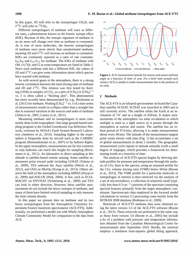
Figure 1. ACE measurement latitude for sunrise and sunset and beta

angle as a function of time of year. For a brief time around each

solstice ACE is unable to make measurements due to the position of

its orbit.

2 Methods

The ACE-FTS is an infrared spectrometer on board the Cana-

dian satellite SCISAT. SCISAT was launched in 2003 and is

still currently active. The satellite orbits the Earth at an in-

clination of 74◦ and at a height of 650 km. It makes mea-

surements of the atmosphere via solar occultation in which

sunlight is used as a light source as it passes through the

atmosphere at sunrise and sunset. The satellite has an or-

bital period of 97.6 min, allowing it to make measurements

about every 49 min. The latitude of the measurement tangent

point varies slowly with time (Fig. 1) but accumulates a set

of global measurements in about 2 months. The geographic

measurement cycle repeats in latitude annually (with a small

degree of slippage), which provides a framework for deter-

mining trends as a function of time.

The analysis of ACE-FTS spectra begins by deriving alti-

tude profiles for pressure and temperature through the analy-

sis of CO2 lines in the spectra, using an assumed profile for

the CO2 volume mixing ratio (VMR) below 60 km (Boone

et al., 2013). The VMR profile for a particular molecule or

isotopologue of interest is then retrieved via the analysis of

a set of microwindows: a collection of relatively small (typi-

cally less than 0.5 cm−1) portions of the spectrum containing

spectral features primarily from the target atmospheric con-

stituent. Spectroscopic data employed in the forward model

calculations in version 3.5 processing come mostly from the

HITRAN 2008 database (Rothman et al., 2009).

Retrievals of ACE-FTS methane data were obtained us-

ing the latest version 3.5 of the ACE-FTS software (Boone

et al., 2013). These retrievals are performed in the same way

as those from version 3.0 (Boone et al., 2005) but include

a fix of a problem with pressure and temperature informa-

tion obtained from the Canadian Meteorological Center for

measurements after September 2010. Briefly, the retrieval

employs a nonlinear least-squares global fitting approach,

Atmos. Meas. Tech., 9, 1095–1111, 2016 www.atmos-meas-tech.net/9/1095/2016/

E. M. Buzan et al.: Global methane isotopologues from ACE-FTS 1097

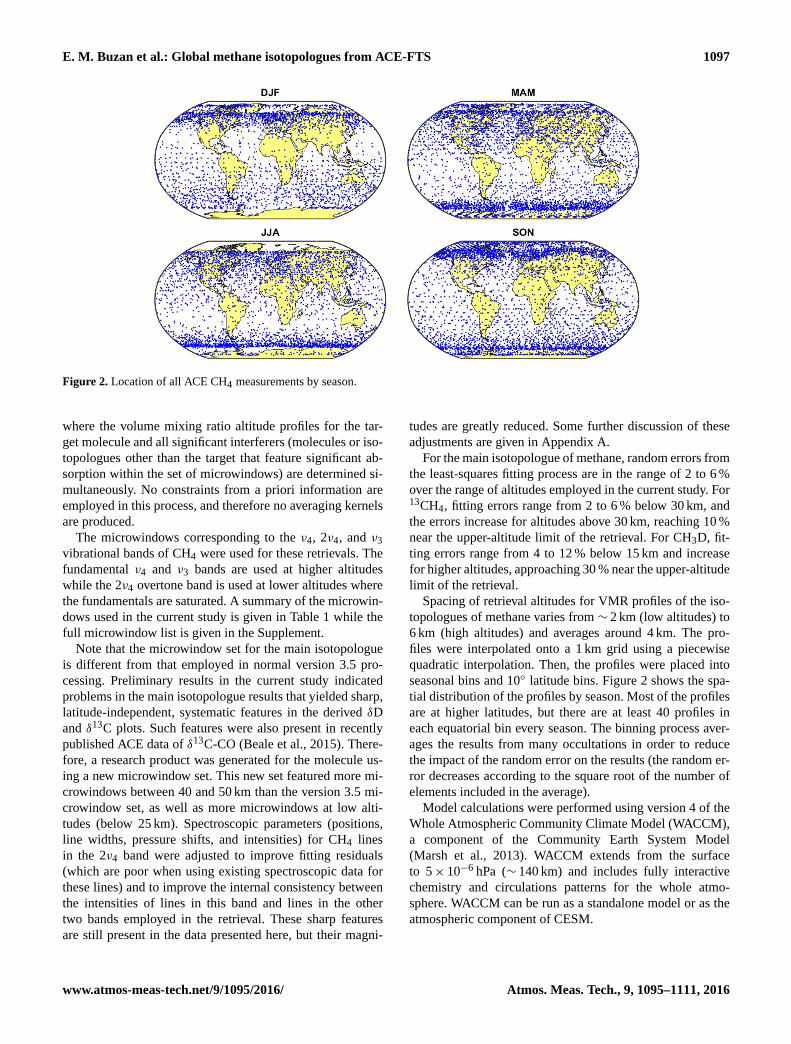
Figure 2. Location of all ACE CH4 measurements by season.

where the volume mixing ratio altitude profiles for the tar-

get molecule and all significant interferers (molecules or iso-

topologues other than the target that feature significant ab-

sorption within the set of microwindows) are determined si-

multaneously. No constraints from a priori information are

employed in this process, and therefore no averaging kernels

are produced.

The microwindows corresponding to the ν4, 2ν4, and ν3

vibrational bands of CH4 were used for these retrievals. The

fundamental ν4 and ν3 bands are used at higher altitudes

while the 2ν4 overtone band is used at lower altitudes where

the fundamentals are saturated. A summary of the microwin-

dows used in the current study is given in Table 1 while the

full microwindow list is given in the Supplement.

Note that the microwindow set for the main isotopologue

is different from that employed in normal version 3.5 pro-

cessing. Preliminary results in the current study indicated

problems in the main isotopologue results that yielded sharp,

latitude-independent, systematic features in the derived δD

and δ13C plots. Such features were also present in recently

published ACE data of δ13C-CO (Beale et al., 2015). There-

fore, a research product was generated for the molecule us-

ing a new microwindow set. This new set featured more mi-

crowindows between 40 and 50 km than the version 3.5 mi-

crowindow set, as well as more microwindows at low alti-

tudes (below 25 km). Spectroscopic parameters (positions,

line widths, pressure shifts, and intensities) for CH4 lines

in the 2ν4 band were adjusted to improve fitting residuals

(which are poor when using existing spectroscopic data for

these lines) and to improve the internal consistency between

the intensities of lines in this band and lines in the other

two bands employed in the retrieval. These sharp features

are still present in the data presented here, but their magni-

tudes are greatly reduced. Some further discussion of these

adjustments are given in Appendix A.

For the main isotopologue of methane, random errors from

the least-squares fitting process are in the range of 2 to 6 %

over the range of altitudes employed in the current study. For13CH4, fitting errors range from 2 to 6 % below 30 km, and

the errors increase for altitudes above 30 km, reaching 10 %

near the upper-altitude limit of the retrieval. For CH3D, fit-

ting errors range from 4 to 12 % below 15 km and increase

for higher altitudes, approaching 30 % near the upper-altitude

limit of the retrieval.

Spacing of retrieval altitudes for VMR profiles of the iso-

topologues of methane varies from ∼ 2 km (low altitudes) to

6 km (high altitudes) and averages around 4 km. The pro-

files were interpolated onto a 1 km grid using a piecewise

quadratic interpolation. Then, the profiles were placed into

seasonal bins and 10◦ latitude bins. Figure 2 shows the spa-

tial distribution of the profiles by season. Most of the profiles

are at higher latitudes, but there are at least 40 profiles in

each equatorial bin every season. The binning process aver-

ages the results from many occultations in order to reduce

the impact of the random error on the results (the random er-

ror decreases according to the square root of the number of

elements included in the average).

Model calculations were performed using version 4 of the

Whole Atmospheric Community Climate Model (WACCM),

a component of the Community Earth System Model

(Marsh et al., 2013). WACCM extends from the surface

to 5× 10−6 hPa (∼ 140 km) and includes fully interactive

chemistry and circulations patterns for the whole atmo-

sphere. WACCM can be run as a standalone model or as the

atmospheric component of CESM.

www.atmos-meas-tech.net/9/1095/2016/ Atmos. Meas. Tech., 9, 1095–1111, 2016

1098 E. M. Buzan et al.: Global methane isotopologues from ACE-FTS

Table 1. Summary of microwindows used by ACE for retrieval of CH4.

Isotopologue Number of Altitude Wave number ranges (cm−1)

microwindows range (km)

CH4 74 5–75 1139, 1219–1374, 1672, 1876, 1950, 2610–3086

CH3D 45 5–35 923–1480, 2623–309613CH4 36 5–50 1202–1339, 1950, 2566–2839

Table 2. Kinetic isotope effect ratios of methane with OH, O1D, and Cl.

Reactant KH/kD k12/k13 Temperature Ref.

OH 1.294± 0.018 1.0039± 0.0004 296 K Saueressig et al. (2001)

O1D 1.06 1.013 296 K Saueressig et al. (2001)

Cl 1.47± 0.03 1.06± 0.01 298 K Feilberg et al. (2005)

Out of the box, WACCM does not support molecular iso-

topologues, but the two isotopologues of CH4 can be inserted

as separate species with a few modifications. First, the re-

actions of the first step of methane oxidation are duplicated

and their rate constants adjusted by the kinetic isotope effects

kD/kH and k12/k13. The KIE of methane with each oxidant

is given in Table 2 and the full set of modified reactions is

listed in Table 3. No further reactions or molecules are mod-

ified as only the isotopic composition of methane is studied

here. Next, new photolytic cross sections were added for all

three isotopologues (Lee et al., 2001; Nair et al., 2005). The

blue shifts of the cross sections are approximately 1 nm for

CH3D and 0.04 nm for 13CH4. Finally, boundary conditions

representing surface emissions were calculated for the two

heavy isotopologues. Keeling plots presented by Röckmann

et al. (2011) were used to derive relations between [CH4] vs.

δD and δ13C:

δD=1.50× 104

[CH4]/(ppm)− 55.6‰, (2)

δ13C=1.29× 104

[CH4]/(ppm)− 151.4‰. (3)

These relations were applied to the existing CH4 boundary

conditions used by WACCM (Lamarque et al., 2010) to de-

rive boundary conditions for CH3D and 13CH4.

WACCM was run as a standalone model with a resolu-

tion of 4× 5◦ (latitude/longitude) and 66 vertical levels. The

model was run as a perpetual year 2000 for a total of 20 years:

17 years of spin-up time followed by 3 years that were ana-

lyzed. Data from WACCM was analyzed in two ways. First,

to observe general trends, the entire data set from the final

3 years was averaged monthly and placed into 10◦ latitude

bins. Second, to remove sampling bias from ACE when com-

paring to WACCM, a smaller data set was constructed by

measuring “profiles” from the whole WACCM data set at the

same times and locations as each ACE profile. This data set

was averaged seasonally and placed into 10◦ latitude bins to

match the analysis of ACE data.

3 Results

Figure 3 shows the total concentration of methane as a func-

tion of latitude and altitude as measured by ACE. In the well-

mixed troposphere, the concentration of methane is nearly

constant at around 1750 ppb. Above the tropopause, methane

concentrations decrease steadily at higher altitudes to about

300 ppb at 20–25 km above the tropopause. Methane near

the equator extends higher into the atmosphere primarily

due to the higher tropopause, as well as the transport of

air containing elevated levels of methane from the tropo-

sphere to the lower stratosphere in the tropics (as part of

the Brewer–Dobson circulation). Some seasonal variation is

visible. Pockets of methane-depleted air are present over the

poles especially during the summer and fall months: Decem-

ber to May over the South Pole and June to November over

the North Pole.

ACE data for δD as a function of latitude and altitude

are plotted in Fig. 4. CH3D data are available from 5 to

30–35 km, depending on latitude. Above 12 km, values of

δD steadily increase with altitude from tropospheric values

around 0 ‰, then sharply increase at the highest few kilome-

ters of the available data to between+250 and+400 ‰. This

sharp increase occurs at the same altitudes where the fitting

errors during retrieval are the highest. In addition, high lev-

els of CH3D are noticeably present over the South Pole from

June to November. Below 12 km, the δD data are much nois-

ier and average around +35‰. This “step function” in the

plot, with a sharp change in δD at a particular altitude that

does not vary with latitude, likely indicates a problem in the

retrieval below 12 km for either CH3D or the main isotopo-

logue. An additional horizontal line is present around 20 km

and is discussed with δ13C below. Finally, there is another

artifact present below 80◦ S in June–August: a single alti-

Atmos. Meas. Tech., 9, 1095–1111, 2016 www.atmos-meas-tech.net/9/1095/2016/

E. M. Buzan et al.: Global methane isotopologues from ACE-FTS 1099

Table 3. Kinetic constants of reactions modified to include the heavy isotopologues of methane used with WACCM. Temperature-independent

reactions use a single rate constant A in units of cm3 molecule−1 s−1. Temperature-dependent reactions have a rate constant given by the

equation k(T )= A× exp(−E/RT ). The factor E/R has units of K−1.

Reaction A E/R Ref.

CH4+OH→ CH3+H2O 2.45× 10−12 1775 Sander et al. (2006)13CH4+OH→ CH3+H2O 2.44× 10−12 1775 Sander et al. (2006)

CH3D +OH→ CH3+H2O 3.50× 10−12 1950 Sander et al. (2006)

CH4+Cl→ CH3+HCl 7.30× 10−12 1280 Sander et al. (2006)13CH4+Cl→ CH3+HCl 6.89× 10−12 1280 Sander et al. (2006)

CH3D +Cl→ CH3+HCl 7.00× 10−12 1380 Feilberg et al. (2005)

CH4+O(1D)→ CH3+OH 1.31× 10−10 Sander et al. (2006)

CH4+O(1D)→ CH2O +H +HO2 3.00× 10−11 Sander et al. (2006)

CH4+O(1D)→ CH2O +H2 7.50× 10−12 Sander et al. (2006)13CH4+O(1D)→ CH3+OH 1.11× 10−10 Saueressig et al. (2001)13CH4+O(1D)→ CH2O +H +HO2 2.96× 10−11 Saueressig et al. (2001)13CH4+O(1D)→ CH2O +H2 7.40× 10−12 Saueressig et al. (2001)

CH3D +O(1D)→ CH3+OH 1.06× 10−10 Saueressig et al. (2001)

CH3D +O(1D)→ CH2O +H +HO2 2.83× 10−11 Saueressig et al. (2001)

CH3D +O(1D)→ CH2O +H2 7.08× 10−12 Saueressig et al. (2001)

CH4+ hν→ products Lee et al. (2001)13CH4+ hν→ products Lee et al. (2001)

CH3D + hν→ products Nair et al. (2005)

Figure 3. ACE total methane concentration by season.

www.atmos-meas-tech.net/9/1095/2016/ Atmos. Meas. Tech., 9, 1095–1111, 2016

1100 E. M. Buzan et al.: Global methane isotopologues from ACE-FTS

Figure 4. ACE δD by season.

Figure 5. ACE δ13C by season.

Atmos. Meas. Tech., 9, 1095–1111, 2016 www.atmos-meas-tech.net/9/1095/2016/

E. M. Buzan et al.: Global methane isotopologues from ACE-FTS 1101

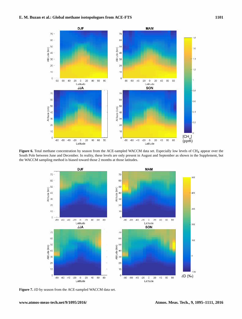
Figure 6. Total methane concentration by season from the ACE-sampled WACCM data set. Especially low levels of CH4 appear over the

South Pole between June and December. In reality, these levels are only present in August and September as shown in the Supplement, but

the WACCM sampling method is biased toward those 2 months at those latitudes.

Figure 7. δD by season from the ACE-sampled WACCM data set.

www.atmos-meas-tech.net/9/1095/2016/ Atmos. Meas. Tech., 9, 1095–1111, 2016

1102 E. M. Buzan et al.: Global methane isotopologues from ACE-FTS

Figure 8. δ13C by season from the ACE-sampled WACCM data set.

tude with a very low δD. This is due to the low number and

quality of measurements taken over the poles caused by the

satellite’s non-polar orbit.

ACE data for δ13C are plotted in Fig. 5. These data are

available from 6 to 50 km except over the poles during some

seasons. Overall the data are noisier than for δD, but values of

δ13C still increase with altitude. Tropospheric values average

near −20 ‰ , while lower stratospheric values average near

0 ‰. Seasonal changes are also more apparent than in δD.

Enrichment of 13C is strongest during the summer and fall

months. Values of δ13C as high as +100 ‰ are present over

both poles between 35 and 50 km. Higher δ13C values are

present in two bands at 22 and 40 km. Since these bands show

no variation in altitude as a function of latitude, they are also

believed to be artifacts of the retrieval process.

Note that there was a very large step function in the orig-

inal version 3.5 δ13C results around 22 and 40 km, a con-

sequence of poor internal consistency between the spectro-

scopic data for the CH4 lines used to derived CH4 VMR at

low altitudes and the CH4 lines used for the high-altitude

portion of the retrieval. This also affected δD, resulting in

a band at around 20 km. For the CH4 research product em-

ployed in the current study, the intensities of CH4 lines in the

2ν4 band (the lines that contribute to retrieved CH4 VMR at

low altitude) were adjusted in an effort to improve the agree-

ment with other CH4 bands employed in the retrieval (i.e.,

the bands that contribute to the retrieved VMR at higher alti-

tudes). The step function in the ACE δ13C results was greatly

reduced, but the “bump” in δ13C near 22 km suggests that

there may remain a spectroscopic compatibility problem for

CH4 lines in different bands. These features also appear in

ACE observations of δ13C–CO (Beale et al., 2015) for the

same reason, suggesting that they are artifacts of the retrieval.

The ACE-sampled WACCM data set is presented in Fig. 6

(total CH4), Fig. 7 (δD), and Fig. 8 (δ13C). Figures of the

full WACCM data set are present in the Supplement. The

model output of total methane agrees well with ACE’s obser-

vations. Tropospheric methane fluctuates slightly by season

but is steady around 1700 ppb. The plume of methane-rich

air over the equator in the stratosphere is also present, and

mixing ratios of methane decrease with higher altitudes in

the stratosphere and mesosphere. Seasonal variation is no-

ticeable here; air masses low in methane form over each pole

around 50 km during the summer, then sink and become fur-

ther depleted during the fall.

These seasonal trends are especially visible in δD and

δ13C. The polar air masses of depleted CH4 are enriched in

both CH3D and 13CH4 and become further enriched as they

sink. Enrichment in the southern air mass reaches a lower al-

titude and lingers for a longer period, February to June, than

the northern air mass which is enriched only from July to

October. This difference in altitude is also shown in ACE;

enrichment in the Southern Hemisphere reaches low enough

Atmos. Meas. Tech., 9, 1095–1111, 2016 www.atmos-meas-tech.net/9/1095/2016/

E. M. Buzan et al.: Global methane isotopologues from ACE-FTS 1103

Figure 9. Keeling plots of ACE data for δD (left) and δ13C (right). Each data point is color-coded by its measurement altitude. The streaks of

data present in the right figure are artifacts; ACE measurements are retrieved to three significant figures, causing a sharp change in precision

around 10 ppm−1 (e.g., 9.99 ppm vs. 10.1 ppm).

to be detected by ACE, while enrichment in the Northern

Hemisphere remains too high to be measurable by ACE.

4 Discussion

4.1 Keeling plots of ACE data

As mentioned previously, the total concentration of atmo-

spheric methane has an inverse relationship with δD and δ13C

as shown in a Keeling plot. Keeling plots for both isotopo-

logues are given in Fig. 9 by plotting the reciprocal of the

methane mixing ratio against δD and δ13C for each altitude

in every ACE profile. In these figures, the expected relation-

ship should appear as a sloped line. Such a slope is visible for

δD at stratospheric altitudes. However, there is still a signifi-

cant range of δD values for a given mixing ratio of methane,

especially in the troposphere where methane has little spa-

tial variability due to being well mixed. For 13CH4, a rela-

tionship between total methane and δ13C is much more dif-

ficult to distinguish. This is not surprising considering that

the δ13C data have a larger range of values than the δD data.

Several streaks are also visible in the δ13C data but are con-

sidered artifacts; since molecular concentrations from ACE

are reported to three significant figures, a sharp change in

precision occurs at multiples of 10, causing the data points

to clump together into lines at just above 10 ppm. A similar

artifact is slightly visible in δD at 1 ppm.

4.2 Comparison to WACCM output

In general, ACE and WACCM have good qualitative agree-

ment with each other. The most noticeable shared feature be-

tween the two is the presence of masses of enriched isotopes

over the poles. In the ACE data for CH3D, the only visible

seasonal change is an increase in δD over the South Pole dur-

ing the winter (JJA). WACCM also shows this enrichment at

the same time. Enrichment over the North Pole is not visible

in the ACE data, but WACCM shows that CH3D enriched

air does not descend to altitudes low enough to be measur-

able with ACE. In addition, the rapid increase in enrichment

at the highest altitudes, 30–35 km, measured by ACE at all

latitudes is not present at the same location in WACCM. In-

creased enrichment is observable above 40 km in WACCM,

but the magnitude of this increase is much smaller. This sug-

gests that the feature in ACE is not a real phenomenon, but

rather it is possibly some systematic effect associated with

the data near the upper-altitude limit of the CH3D retrievals,

a consequence of pushing the retrievals to altitudes where the

spectra contain minimal signal from the isotopologue.

Though δ13C data from ACE are much noisier than for δD,

seasonal enrichment over both poles is visible as the δ13C

data extend to high altitudes. In both ACE and WACCM,

enrichment over the South Pole is most visible in the fall

(MAM) months with slightly lower enrichment during the

winter (JJA) and spring (SON). The same trend is present

over the North Pole in the fall (SON), but again the amount

of enrichment fades more rapidly with time as it did with

CH3D.

www.atmos-meas-tech.net/9/1095/2016/ Atmos. Meas. Tech., 9, 1095–1111, 2016

1104 E. M. Buzan et al.: Global methane isotopologues from ACE-FTS

Figure 10. The difference in δD between ACE and WACCM. Negative values are given when ACE reports a larger value than WACCM.

However, ACE and WACCM disagree greatly over the val-

ues of δD and δ13C. ACE reports values of δ13C of over

+100 ‰ in highly enriched areas, while WACCM reports

δ13C values only up to +5 ‰ at the altitudes measured by

ACE. Tropospheric values are closer, but there is still a dis-

parity: ACE measures δ13C around −20 ‰ while WACCM

reports it at around −45 ‰. The difference is more pro-

nounced with δD. Tropospheric values of δD differ by 100 ‰

between ACE and WACCM. A quantitative comparison of

δD in the stratosphere is more difficult due to the sharp in-

crease seen in ACE.

Systematic errors in the ACE CH4 results are clearly dom-

inated by errors in the spectroscopic constants. Although dra-

matically improved compared to the preliminary results that

used the version 3.5 processing, there remain sharp latitude-

independent features at particular altitudes in the fractiona-

tion plots in the current study using the research product for

main isotopologue CH4. While the new spectroscopic param-

eters derived for the main isotopologue of CH4 significantly

improve the fitting residuals and reduce the magnitudes of

the sharp features in the fractionation plots, further work is

clearly required to refine the quality of these spectroscopic

constants. It is not clear at this time what contributions to the

systematic features are from the main isotopologue vs. the

subsidiary isotopologues. With the magnitudes of the uncer-

tainties involved, there seems little value in generating a for-

mal, quantitative estimate of the systematic error; the errors

are large enough (the δD curve was more than 9 % different

from expectations, and the δ13C curve was more than 2 % dif-

ferent) to necessitate generating new spectroscopic constants

for at least some portion of the CH4 lines in the microwin-

dows employed for the ACE-FTS retrievals.

4.3 Calibration of ACE data

In the troposphere, WACCM’s predictions of δD and δ13C

agree with previous measurements. For δ13C, WACCM pre-

dicts a tropospheric value of −47 ‰, while measurements

range from −48 to −46 ‰ (Conny and Currie, 1996; Sug-

awara et al., 1997; Umezawa et al., 2012). Tropospheric

δD measurements have a larger range, between −100 and

−75 ‰ (Rice et al., 2003; Umezawa et al., 2012). WACCM

lies on the high end of this, between −81 and −78 ‰ , with

more a negative δD in the Northern Hemisphere. Based on

this agreement, WACCM can be used to calibrate ACE by

accounting for the unknown systemic error in the ACE re-

trievals of CH3D and 13CH4. These calibration factors, one

for each isotopologue, are a shift applied to δD and δ13C

from ACE and are equivalent to a multiplication factor ap-

plied to the CH3D and 13CH4 VMR profiles retrieved by

ACE. The calibration factors were derived by taking the dif-

ference of the median tropospheric δ value for both isotopo-

logues of ACE and WACCM. The height of the tropopause

for each ACE profile was taken from derived meteorologi-

cal products provided by Manney et al. (2007) and was be-

tween 8 and 16 km for most profiles. The calculated calibra-

tion shifts are −92.4 ‰ for δD and −21.8 ‰ for δ13C.

Atmos. Meas. Tech., 9, 1095–1111, 2016 www.atmos-meas-tech.net/9/1095/2016/

E. M. Buzan et al.: Global methane isotopologues from ACE-FTS 1105

Figure 11. The difference in δ13C between ACE and WACCM. Negative values are given when ACE reports a larger value than WACCM.

The effect of this calibration at one location, the 60◦ S

ACE latitude bin during the spring (SON), is shown in

Fig. 12. Also shown here are error bars on the post-

calibration ACE data. These error bars represent 1 standard

deviation of measurements from the entire data set at that al-

titude and latitude bin. The calibration is effective for CH3D

as ACE and WACCM now agree with each other up to 26 km

where the sharp increase in δD is observed in ACE. How-

ever, this calibration does not function as well for 13CH4.

After the calibration, ACE and WACCM agree up to a height

of about 20 km, but the bump in the ACE results between 20

and 25 km (associated with the latitude-independent band in

the δ13C plots near 22 km mentioned previously) yields sig-

nificantly poorer agreement in that altitude range. The ACE

results also show a stronger increase of δ13C with increasing

altitude above 20 km compared to WACCM.

4.4 Comparison to balloon profiles

ACE data were compared with balloon profiles analyzed by

Röckmann et al. (2011). This data set consists of 13 balloon

profiles, all of which have data for δ13C and all but two have

data for δD. The balloon launches were performed at Hyder-

abad, India (17.5◦ N, 78.60◦ E), Kiruna, Sweden (67.9◦ N,

21.10◦ E), Aire-sur-l’Adour, France (43.70◦ N, −0.30◦ E),

and Gap, France (44.44◦ N, 6.14◦ E). The balloon profiles

from each location were compared to ACE profiles from the

same season and the 10◦ latitude bin the balloon launches are

located in. Both locations in France were considered together

since only one launch was performed at Gap.

Figure 13 shows the comparison of δD among ACE

(shown in red), WACCM (gray and black), and the balloon

profiles (blue). The profiles over India and both locations

in France show strong agreement among all three data sets

to above 25 km. Over India, the balloon profiles end below

30 km, so there are no data to compare to the highest altitudes

of ACE where δD rapidly increases. Over France, the balloon

profiles reach as high as 33 km, slightly higher than ACE, but

do not show the spike in δD present in ACE. This, along with

the high amount of random error present in the retrieval at

this altitude, supports the notion that the rapid increase in δD

at the highest altitudes in the ACE results is a retrieval arti-

fact. One profile, ASA9309, does show increased δD at the

single highest point, but this is not conclusive. However, the

profiles over Sweden do not show such agreement. Above

20 km, the balloon profiles show a large increase and notice-

able month-to-month changes in δD, whereas ACE shows a

more gradual rise. The sharp increase is likely due to strong

influence from the polar vortex during the 2 years of mea-

surements. The ACE data are a combination of 10 years

of profiles, so years of strong vortex influence are balanced

by years with less influence. Also, the run of WACCM does

not include any interannual variation, so the effect of an av-

erage polar vortex is expected.

Figure 14 shows the comparison of the three data sets

for δ13C. Quantitatively, agreement is generally poorer be-

tween ACE and the balloon profiles than was observed for

www.atmos-meas-tech.net/9/1095/2016/ Atmos. Meas. Tech., 9, 1095–1111, 2016

1106 E. M. Buzan et al.: Global methane isotopologues from ACE-FTS

Figure 12. Results of ACE calibration compared to WACCM. Data shown here are from the 60◦ S September/October/November data bin.

The error bars on the calibrated ACE data are equal to 1 standard deviation of the measurements at that altitude.

Figure 13. Comparison of δD profiles from ACE before and after calibration, WACCM, and balloon profiles from Röckmann et al. (2011).

Atmos. Meas. Tech., 9, 1095–1111, 2016 www.atmos-meas-tech.net/9/1095/2016/

E. M. Buzan et al.: Global methane isotopologues from ACE-FTS 1107

Figure 14. Comparison of δ13C profiles from ACE before and after calibration, WACCM, and balloon profiles from Röckmann et al. (2011).

δD. Excluding the apparent artifact in the ACE δ13C re-

sults (the bump between 20 and 25 km), there is reasonable

agreement for the balloon measurements over India. For the

higher-latitude measurements over France and Sweden, ACE

indicates a smaller isotopic fractionation in the troposphere

than was measured by the balloon campaign or predicted by

WACCM. Interestingly, the balloon measurements in Swe-

den show fairly good agreement with the bump between 20

and 25 km in the ACE δ13C results, but since this bump in

the ACE results is thought to be an artifact, this agreement is

probably a coincidence.

4.5 Distribution of methane sinks

A second set of WACCM runs was performed to further ex-

plore the effects of the different sinks of methane on its iso-

topic composition. The model was run an additional year past

the initial 20 years. Then, several 1-day branch runs were

performed on the first day of each month of the extra year.

In these runs, the reactions for methane with OH, O (1D),

Cl, and sunlight (photolysis) were modified to additionally

produce an inert dummy molecule. The abundance of this

“molecule” at a specific location shows how much methane

reacted with a specific molecule or via photolysis at that lo-

cation. Since the model reports molecular concentrations as

mixing ratios, the abundance of the dummy molecules is rel-

ative to the number density of air at that location. The mixing

ratios of the dummy molecules are on the order of 10−9 or

smaller, so their presence does not have a large effect on the

pressure or other dynamics in the atmosphere.

Figure 15 shows the results of these runs for the months

of January, April, July, and October. The plots in the left col-

umn show which of the four sinks destroys the most methane

at a given latitude and altitude. The right column shows the

total rate of methane destruction. At the most abundant rad-

ical in the atmosphere, OH is the most important oxidant in

the troposphere and most of the stratosphere outside of the

polar regions. From 50 to 65 km, singlet oxygen becomes

the largest oxidant. It is also the largest oxidant between 30

and 40 km at the equator, likely due to the presence of the

ozone layer below which readily photolyzes to give oxygen

atoms. Above 65 km, photolysis becomes the major source

of methane destruction as the atmosphere becomes thinner,

making chemical reactions more difficult and allowing the

increased penetration of UV radiation.

www.atmos-meas-tech.net/9/1095/2016/ Atmos. Meas. Tech., 9, 1095–1111, 2016

1108 E. M. Buzan et al.: Global methane isotopologues from ACE-FTS

Figure 15. Dominant oxidizing species of CH4 by location and sea-

son (left) and total methane oxidation (right).

The reaction of methane with chlorine atoms demonstrates

strong seasonal variation. Oxidation via chlorine is only

major over the poles in the stratosphere around the winter

months. At the same time over the poles, methane destruction

reaches its lowest rates. This is due to the presence of the po-

lar vortex. The isolated air inside the vortex is not exposed to

sunlight, so oxidizing radicals are quickly consumed and are

not regenerated. Meanwhile, active chlorine-containing com-

pounds build up within the vortex, providing a small source

of chlorine atoms even with minimal sunlight.

5 Conclusions

The ACE data set presented in this paper greatly expands the

number of observations of methane and its isotopologues in

the stratosphere. The data for CH3D have been shown to be

consistent with both model predictions and existing balloon-

based measurements after calibrating the ACE results using

tropospheric δD calculated from the WACCM model. How-

ever, the data for 13CH4 still show large discrepancies. The

addition of new microwindows and adjustment of spectro-

scopic parameters for CH4 lines in the 2ν4 band significantly

reduced the large step function observed in δ13C when using

the spectroscopic parameters for this band that are currently

available in the HITRAN database. However, a systematic

latitude-independent bump near 22 km in the δ13C profiles

derived from ACE in the current study suggests that further

refinement of these spectroscopic constants will be required

to improve the retrieval results for the isotopologues CH4

from ACE.

Atmos. Meas. Tech., 9, 1095–1111, 2016 www.atmos-meas-tech.net/9/1095/2016/

E. M. Buzan et al.: Global methane isotopologues from ACE-FTS 1109

Appendix A

The adjusted spectroscopic parameters generated for CH4

from ACE-FTS spectra are collected in the Supplement. Only

those parameters that differ from the values in HITRAN 2004

are included. All units are the standard HITRAN units (Roth-

man et al., 2005). Spectroscopic parameters were adjusted

primarily for the CH4 lines contained in the main isotopo-

logue microwindow set. One adjustment made was an in-

crease of the intensities in the low-altitude lines by more than

3 %. Not all CH4 in the given wave number region were ad-

justed, and no changes were made to the parameters for the

subsidiary isotopologues.

It should be stressed that although these new parameters

do significantly improve the fitting residuals and give vol-

ume mixing ratio profiles that yield variations with altitude

that match more closely with expectations, an occultation

sounder is not the ideal platform for generating spectroscopic

parameters. Rather than a static cell, as one would have in

a laboratory, there is a variation along the line of sight for

pressure and temperature. Contribution to the residuals from

imperfectly modeled interferences (i.e., molecules other than

CH4) would impact the determination of CH4 spectroscopic

parameters. The range of temperatures for the measurements

is insufficient to properly generate spectroscopic parameters

that describe temperature dependence, and so such parame-

ters were all fixed to the values in HITRAN 2004.

It is clear that CH4 would benefit greatly from new labo-

ratory studies, particularly in the 2650 cm−1 region for the

main isotopologue. The sharp features at a particular alti-

tude in the fractionation plots indicate that problems with

the spectroscopic parameters are the dominant source of sys-

tematic error in this study. For all isotopologues, retrievals

for CH4 in different altitude regions are derived from dif-

ferent spectroscopic bands, and inconsistencies in the spec-

troscopy for the different bands generate sharp “steps” in the

retrieved profiles. Isotope studies are sensitive to these sys-

tematic steps, making such studies an excellent tool for eval-

uating the internal consistency of the spectroscopy for the

isotopologues involved.

This study illustrated a significant problem with the inter-

nal consistency of spectroscopic constants in different bands

of CH4. The new CH4 spectroscopic parameters reported

here reduce that inconsistency, but problems remain. At this

time, it is unclear whether the remaining systematic features

in the fractionation plots arise primarily from the subsidiary

isotopologues, from the main isotopologue, or some combi-

nation thereof.

www.atmos-meas-tech.net/9/1095/2016/ Atmos. Meas. Tech., 9, 1095–1111, 2016

1110 E. M. Buzan et al.: Global methane isotopologues from ACE-FTS

The Supplement related to this article is available online

at doi:10.5194/amt-9-1095-2016-supplement.

Acknowledgements. The ACE mission is funded primarily by the

Canadian Space Agency. This project was initiated during a visit

by P. Bernath to the National Center of Atmospheric Research

(NCAR) in Boulder, CO, and the help with WACCM provided by

D. Kinnison, D. Marsh, and M. Mills is gratefully acknowledged.

We thank T. Röckmann for supplying the methane isotopologue

data from balloon measurements.

Edited by: F. Hase

References

Allan, W., Manning, M. R., Lassey, K. R., Lowe, D. C., and Gomez,

A. J.: Modeling the variation of δ13C in atmospheric methane:

Phase ellipses and the kinetic isotope effect, Global Biogeochem.

Cy., 15, 467–481, doi:10.1029/2000GB001282, 2001.

Andrews, A. E., Kofler, J. D., Trudeau, M. E., Williams, J. C., Neff,

D. H., Masarie, K. A., Chao, D. Y., Kitzis, D. R., Novelli, P.

C., Zhao, C. L., Dlugokencky, E. J., Lang, P. M., Crotwell, M.

J., Fischer, M. L., Parker, M. J., Lee, J. T., Baumann, D. D.,

Desai, A. R., Stanier, C. O., De Wekker, S. F. J., Wolfe, D. E.,

Munger, J. W., and Tans, P. P.: CO2, CO, and CH4 measure-

ments from tall towers in the NOAA Earth System Research

Laboratory’s Global Greenhouse Gas Reference Network: instru-

mentation, uncertainty analysis, and recommendations for future

high-accuracy greenhouse gas monitoring efforts, Atmos. Meas.

Tech., 7, 647–687, doi:10.5194/amt-7-647-2014, 2014.

Bartlett, K. B. and Harriss, R. C.: Review and assessment of

methane emissions from wetlands, Chemosphere, 26, 261–320,

doi:10.1016/0045-6535(93)90427-7, 1993.

Beale, C. A., Buzan, E. M., Boone, C. D., and Bernath,

P. F.: Near-global distribution of CO isotopic fractiona-

tion in the Earth’s atmosphere, J. Mol. Spectrosc., 1–8,

doi:10.1016/j.jms.2015.12.005, 2015.

Boone, C. D., Nassar, R., Walker, K. A., Rochon, Y., McLeod, S.

D., Rinsland, C. P., and Bernath, P. F.: Retrievals for the at-

mospheric chemistry experiment Fourier-transform spectrome-

ter, Appl. Opt., 44, 7218, doi:10.1364/AO.44.007218, 2005.

Boone, C. D., Walker, K. A., and Bernath, P. F.: Version 3 Retrievals

of the Atmospheric Chemistry Experiment Fourier Transform

Spectrometer (ACE-FTS), in: The Atmospheric Chemistry Ex-

periment: ACE at 10, edited by: Bernath, P. F., 103–129, A,

Deepak Publishing, Hampton, VA, available at: http://www.ace.

uwaterloo.ca/v1data/Boone-retrievals2005reprint.pdf (last ac-

cess: 26 February 2016), 2013.

Brenninkmeijer, C. A. M., Crutzen, P., Boumard, F., Dauer, T., Dix,

B., Ebinghaus, R., Filippi, D., Fischer, H., Franke, H., Frieß, U.,

Heintzenberg, J., Helleis, F., Hermann, M., Kock, H. H., Koep-

pel, C., Lelieveld, J., Leuenberger, M., Martinsson, B. G., Miem-

czyk, S., Moret, H. P., Nguyen, H. N., Nyfeler, P., Oram, D.,

O’Sullivan, D., Penkett, S., Platt, U., Pupek, M., Ramonet, M.,

Randa, B., Reichelt, M., Rhee, T. S., Rohwer, J., Rosenfeld, K.,

Scharffe, D., Schlager, H., Schumann, U., Slemr, F., Sprung, D.,

Stock, P., Thaler, R., Valentino, F., van Velthoven, P., Waibel, A.,

Wandel, A., Waschitschek, K., Wiedensohler, A., Xueref-Remy,

I., Zahn, A., Zech, U., and Ziereis, H.: Civil Aircraft for the reg-

ular investigation of the atmosphere based on an instrumented

container: The new CARIBIC system, Atmos. Chem. Phys., 7,

4953–4976, doi:10.5194/acp-7-4953-2007, 2007.

Conny, J. M. and Currie, L. A.: The isotopic characterization of

methane, non-methane hydrocarbons and formaldehyde in the

troposphere, Atmos. Environ., 30, 621–638, doi:10.1016/1352-

2310(95)00305-3, 1996.

Denman, K. L., Brasseur, G., Chidthaisong, A., Ciais, P., Cox, P. M.,

Dickinson, R. E., Hauglustaine, D., Heinze, C., Holland, E., Ja-

cob, D., Lohmann, U., Ramachandran, S., Dias, P. L. da S.,

Wofsy, S. C., and Zhang, X.: Couplings between changes in the

climate system and biogeochemistry, in: Climate Change 2007:

The Physical Science Basis. Contribution of Working Group I

to the Fourth Assessment Report of the Intergovernmental Panel

on Climate Change, edited by: Solomon, S., Qin, D., Man-

ning, M., Chen, Z., Marquis, M., Averyt, K. B.,Tignor, M., and

Miller, H. L., Cambridge University Press, Cambridge, UK, 499–

587, 2007.

Etheridge, D. M., Steele, L. P., Francey, R. J., and Langenfelds,

R. L.: Atmospheric methane between 1000 A.D., and present:

Evidence of anthropogenic emissions and climatic variability, J.

Geophys. Res., 103, 15979, doi:10.1029/98JD00923, 1998.

Feilberg, K. L., Griffith, D. W. T., Johnson, M. S., and Nielsen, C. J.:

The 13C and D kinetic isotope effects in the reaction of CH4 with

Cl, Int. J. Chem. Kinet., 37, 110–118, doi:10.1002/kin.20058,

2005.

Hao, W. M. and Ward, D. E.: Methane production from

global biomass burning, J. Geophys. Res., 98, 20657,

doi:10.1029/93JD01908, 1993.

Keeling, C. D.: The concentration and isotopic abundances of at-

mospheric carbon dioxide in rural areas, Geochim. Cosmochim.

Ac., 13, 322–334, doi:10.1016/0016-7037(58)90033-4, 1958.

Kort, E. A., Frankenberg, C., Costigan, K. R., Lindenmaier, R.,

Dubey, M. K., and Wunch, D.: Four corners: The largest US

methane anomaly viewed from space, Geophys. Res. Lett., 41,

6898–6903, doi:10.1002/2014GL061503, 2014.

Lamarque, J.-F., Bond, T. C., Eyring, V., Granier, C., Heil, A.,

Klimont, Z., Lee, D., Liousse, C., Mieville, A., Owen, B.,

Schultz, M. G., Shindell, D., Smith, S. J., Stehfest, E., Van Aar-

denne, J., Cooper, O. R., Kainuma, M., Mahowald, N., Mc-

Connell, J. R., Naik, V., Riahi, K., and van Vuuren, D. P.: His-

torical (1850–2000) gridded anthropogenic and biomass burning

emissions of reactive gases and aerosols: methodology and ap-

plication, Atmos. Chem. Phys., 10, 7017–7039, doi:10.5194/acp-

10-7017-2010, 2010.

Lassey, K. R.: Livestock methane emission: From the indi-

vidual grazing animal through national inventories to the

global methane cycle, Agr. Forest Meteorol., 142, 120–132,

doi:10.1016/j.agrformet.2006.03.028, 2007.

Lassey, K. R., Allan, W., and Fletcher, S. E. M.: Seasonal inter-

relationships in atmospheric methane and companion δ13C val-

ues: Effects of sinks and sources, Tellus, Ser. B Chem. Phys.

Meteorol., 63, 287–301, doi:10.1111/j.1600-0889.2011.00535.x,

2011.

Atmos. Meas. Tech., 9, 1095–1111, 2016 www.atmos-meas-tech.net/9/1095/2016/

E. M. Buzan et al.: Global methane isotopologues from ACE-FTS 1111

Lee, A. Y. T., Yung, Y. L., Cheng, B.-M., Bahou, M., Chung, C.-Y.,

and Lee, Y.-P.: Enhancement of Deuterated Ethane on Jupiter,

Astrophys. J., 551, L93–L96, doi:10.1086/319827, 2001.

Manney, G. L., Daffer, W. H., Zawodny, J. M., Bernath, P. F., Hop-

pel, K. W., Walker, K. A., Knosp, B. W., Boone, C., Rems-

berg, E. E., Santee, M. L., Harvey, V. L., Pawson, S., Jackson,

D. R., Deaver, L., McElroy, C. T., McLinden, C. A., Drum-

mond, J. R., Pumphrey, H. C., Lambert, A., Schwartz, M. J.,

Froidevaux, L., McLeod, S., Takacs, L. L., Suarez, M. J., Trepte,

C. R., Cuddy, D. C., Livesey, N. J., Harwood, R. S., and Wa-

ters, J. W.: Solar occultation satellite data and derived me-

teorological products: Sampling issues and comparisons with

Aura Microwave Limb Sounder, J. Geophys. Res., 112, D24S50,

doi:10.1029/2007JD008709, 2007.

Marsh, D. R., Mills, M. J., Kinnison, D. E., Lamarque, J.-F.,

Calvo, N., and Polvani, L. M.: Climate Change from 1850 to

2005 Simulated in CESM1(WACCM), J. Clim., 26, 7372–7391,

doi:10.1175/JCLI-D-12-00558.1, 2013.

Nair, H., Summers, M., Miller, C., and Yung, Y.: Isotopic fraction-

ation of methane in the martian atmosphere, Icarus, 175, 32–35,

doi:10.1016/j.icarus.2004.10.018, 2005.

Park, M.: Seasonal variation of methane, water vapor, and

nitrogen oxides near the tropopause: Satellite observations

and model simulations, J. Geophys. Res., 109, D03302,

doi:10.1029/2003JD003706, 2004.

Payan, S., Camy-Peyret, C., Oelhaf, H., Wetzel, G., Maucher, G.,

Keim, C., Pirre, M., Huret, N., Engel, A., Volk, M. C., Kuell-

mann, H., Kuttippurath, J., Cortesi, U., Bianchini, G., Mencar-

aglia, F., Raspollini, P., Redaelli, G., Vigouroux, C., De Maz-

ière, M., Mikuteit, S., Blumenstock, T., Velazco, V., Notholt, J.,

Mahieu, E., Duchatelet, P., Smale, D., Wood, S., Jones, N., Pic-

colo, C., Payne, V., Bracher, A., Glatthor, N., Stiller, G., Grunow,

K., Jeseck, P., Te, Y., and Butz, A.: Validation of version-4.61

methane and nitrous oxide observed by MIPAS, Atmos. Chem.

Phys., 9, 413–442, doi:10.5194/acp-9-413-2009, 2009.

Remsberg, E. E.: Methane as a diagnostic tracer of changes in the

Brewer–Dobson circulation of the stratosphere, Atmos. Chem.

Phys., 15, 3739–3754, doi:10.5194/acp-15-3739-2015, 2015.

Rice, A. L., Tyler, S. C., McCarthy, M. C., Boering, K.

A., and Atlas, A.: Carbon and hydrogen isotopic composi-

tions of stratospheric methane: 1. High-precision observations

from the NASA ER-2 aircraft, J. Geophys. Res., 108, 4460,

doi:10.1029/2002JD003042, 2003.

Röckmann, T., Brass, M., Borchers, R., and Engel, A.: The isotopic

composition of methane in the stratosphere: high-altitude balloon

sample measurements, Atmos. Chem. Phys., 11, 13287–13304,

doi:10.5194/acp-11-13287-2011, 2011.

Rothman, L. S., Jacquemart, D., Barbe, A., Chris Benner, D., Birk,

M., Brown, L. R., Carleer, M. R., Chackerian, C., Chance, K.,

Coudert, L. H., Dana, V., Devi, V. M., Flaud, J.-M., Gamache,

R. R., Goldman, A., Hartmann, J.-M., Jucks, K. W., Maki, A. G.,

Mandin, J.-Y., Massie, S. T., Orphal, J., Perrin, A., Rinsland, C.

P., Smith, M. A. H., Tennyson, J., Tolchenov, R. N., Toth, R. A.,

Vander Auwera, J., Varanasi, P., and Wagner, G.: The HITRAN

2004 molecular spectroscopic database, J. Quant. Spectrosc. Ra.,

96, 139–204, doi:10.1016/j.jqsrt.2004.10.008, 2005.

Rothman, L. S., Gordon, I. E., Barbe, A., Benner, D. C., Bernath,

P. F., Birk, M., Boudon, V., Brown, L. R., Campargue, A.,

Champion, J.-P., Chance, K., Coudert, L. H., Dana, V., Devi,

V. M., Fally, S., Flaud, J.-M., Gamache, R. R., Goldman,

A., Jacquemart, D., Kleiner, I., Lacome, N., Lafferty, W. J.,

Mandin, J.-Y., Massie, S. T., Mikhailenko, S. N., Miller, C. E.,

Moazzen-Ahmadi, N., Naumenko, O. V., Nikitin, A. V., Or-

phal, J., Perevalov, V. I., Perrin, A., Predoi-Cross, A., Rins-

land, C. P., Rotger, M., Šimecková, M., Smith, M. A. H., Sung,

K., Tashkun, S. A., Tennyson, J., Toth, R. A., Vandaele, A. C.,

and Vander Auwera, J.: The HITRAN 2008 molecular spec-

troscopic database, J. Quant. Spectrosc. Ra., 110, 533–572,

doi:10.1016/j.jqsrt.2009.02.013, 2009.

Sander, S. P., Friedl, R. R., Golden, D. M., Kurylo, M. J., Moortgat,

G. K., Wine, P. H., Ravishankara, a R., Kolb, C. E., Molina, M.

J., Diego, S., Jolla, L., Huie, R. E., and Orkin, V. L.: Chemical

Kinetics and Photochemical Data for Use in Atmospheric Studies

Evaluation Number 15, JPL Publ., 06-2(Eval. 15), available at:

http://jpldataeval.jpl.nasa.gov/ (last access: 26 February 2016),

2006.

Saueressig, G., Crowley, J. N., Bergamaschi, P., Brühl, C., Bren-

ninkmeijer, C. A. M., and Fischer, H.: Carbon 13 and D kinetic

isotope effects in the reactions of CH4 with O(1D) and OH: New

laboratory measurements and their implications for the isotopic

composition of stratospheric methane, J. Geophys. Res., 106,

23127, doi:10.1029/2000JD000120, 2001.

Schneising, O., Buchwitz, M., Burrows, J. P., Bovensmann, H.,

Bergamaschi, P., and Peters, W.: Three years of greenhouse gas

column-averaged dry air mole fractions retrieved from satel-

lite – Part 2: Methane, Atmos. Chem. Phys., 9, 443–465,

doi:10.5194/acp-9-443-2009, 2009.

Sugawara, S., Nakazawa, T., Shirakawa, Y., Kawamura, K., Aoki,

S., Machida, T., and Honda, H.: Vertical profile of the carbon

isotopic ratio of stratospheric methane over Japan, Geophys. Res.

Lett., 24, 2989–2992, doi:10.1029/97GL03044, 1997.

Terao, Y., Mukai, H., Nojiri, Y., MacHida, T., Tohjima, Y., Saeki,

T., and Maksyutov, S.: Interannual variability and trends in atmo-

spheric methane over the western Pacific from 1994 to 2010, J.

Geophys. Res.-Atmos., 116, 1–13, doi:10.1029/2010JD015467,

2011.

Umezawa, T., Machida, T., Ishijima, K., Matsueda, H., Sawa, Y.,

Patra, P. K., Aoki, S., and Nakazawa, T.: Carbon and hydrogen

isotopic ratios of atmospheric methane in the upper troposphere

over the Western Pacific, Atmos. Chem. Phys., 12, 8095–8113,

doi:10.5194/acp-12-8095-2012, 2012.

Wecht, K. J., Jacob, D. J., Wofsy, S. C., Kort, E. A., Worden, J. R.,

Kulawik, S. S., Henze, D. K., Kopacz, M., and Payne, V. H.: Val-

idation of TES methane with HIPPO aircraft observations: impli-

cations for inverse modeling of methane sources, Atmos. Chem.

Phys., 12, 1823–1832, doi:10.5194/acp-12-1823-2012, 2012.

Xiong, X., Barnet, C., Maddy, E. S., Gambacorta, A., King, T.

S., and Wofsy, S. C.: Mid-upper tropospheric methane retrieval

from IASI and its validation, Atmos. Meas. Tech., 6, 2255–2265,

doi:10.5194/amt-6-2255-2013, 2013.

Yokota, T., Yoshida, Y., Eguchi, N., Ota, Y., Tanaka, T., Watanabe,

H., and Maksyutov, S.: Global Concentrations of CO2 and CH4

Retrieved from GOSAT: First Preliminary Results, Sci. Online

Lett. Atmos., 5, 160–163, doi:10.2151/sola.2009-041, 2009.

www.atmos-meas-tech.net/9/1095/2016/ Atmos. Meas. Tech., 9, 1095–1111, 2016