HAL Id: inria-00581259https://hal.inria.fr/inria-00581259

Submitted on 30 Mar 2011

HAL is a multi-disciplinary open accessarchive for the deposit and dissemination of sci-entific research documents, whether they are pub-lished or not. The documents may come fromteaching and research institutions in France orabroad, or from public or private research centers.

L’archive ouverte pluridisciplinaire HAL, estdestinée au dépôt et à la diffusion de documentsscientifiques de niveau recherche, publiés ou non,émanant des établissements d’enseignement et derecherche français ou étrangers, des laboratoirespublics ou privés.

Distributed under a Creative Commons Attribution| 4.0 International License

Global State Estimates for Distributed SystemsGabriel Kalyon, Tristan Le Gall, Hervé Marchand, Thierry Massart

To cite this version:Gabriel Kalyon, Tristan Le Gall, Hervé Marchand, Thierry Massart. Global State Estimates forDistributed Systems. 13th Conference on Formal Methods for Open Object-Based Distributed Systems(FMOODS) / 31th International Conference on FORmal TEchniques for Networked and DistributedSystems (FORTE), Jun 2011, Reykjavik, Iceland. pp.198-212, �10.1007/978-3-642-21461-5_13�. �inria-00581259�

Global State Estimates for Distributed Systems

Gabriel Kalyon1, Tristan Le Gall2, Herve Marchand3 and Thierry Massart1?1 Universite Libre de Bruxelles (U.L.B.), Campus de la Plaine, Bruxelles, Belgique

2 CEA LIST, LMeASI, boıte 94, 91141 Gif-sur-Yvette, France3 INRIA, Rennes - Bretagne Atlantique, France

Abstract. We consider distributed systems modeled as communicating finite statemachines with reliable unbounded FIFO channels. As an essential sub-routine forcontrol, monitoring and diagnosis applications, we provide an algorithm that com-putes, during the execution of the system, an estimate of the current global stateof the distributed system for each local subsystem. This algorithm does not changethe behavior of the system; each subsystem only computes and records a symbolicrepresentation of the state estimates, and piggybacks some extra information to themessages sent to the other subsystems in order to refine their estimates. Our algo-rithm relies on the computation of reachable states. Since the reachability problem isundecidable in our model, we use abstract interpretation techniques to obtain regularoverapproximations of the possible FIFO channel contents, and hence of the possi-ble current global states. An implementation of this algorithm provides an empiricalevaluation of our method.

1 Introduction

During the execution of a computer system, the knowledge of its global state may be cru-cial information, for instance to control which action can or must be done, to monitor itsbehavior or perform some diagnostic. Distributed systems, are generally divided into twoclasses, depending on whether the communication between subsystems is synchronous ornot. When the synchrony hypothesis [1] can be made, each local subsystem can easilyknow, at each step of the execution, the global state of the system (assuming that thereis no internal action). When considering asynchronous distributed systems, this knowl-edge is in general impossible, since the communication delays between the components ofthe system must be taken into account. Therefore, each local subsystem can a priori notimmediately know either the local state of the other subsystems or the messages that arecurrently in transfer.

In this paper, we are interested in the asynchronous framework where we consider thatthe system is composed of n subsystems that asynchronously communicate through reli-able unbounded FIFO channels. These subsystems are modeled by communicating finitestate machines (CFSM) [4] that explicitly express the work and communications of a dis-tributed system. This model appears to be essential for concurrent systems in which com-ponents cooperate via asynchronous message passing through unbounded buffers (they aree.g. widely used to model communication protocols). We thus assume that the distributedsystem is already built and the architecture of communication between the different sub-systems is fixed. Our aim is to provide an algorithm that allows us to compute, in each? This work has been done in the MoVES project (P6/39), part of the IAP-Phase VI Interuniversity

Attraction Poles Programme funded by the Belgian State, Belgian Science Policy.

subsystem of a distributed system T , an estimate of the current state of T . More precisely,each subsystem or a local associated estimator computes a set of possible global states,including the contents of the channels, in which the system T can be; it can be seen as aparticular case of monitoring with partial observation. In our framework, we assume thatthe subsystems (or associated estimators) can record their own state estimate and that someextra information can be piggybacked to the messages normally exchanged by the subsys-tems. Indeed, without this additional information, since a local subsystem cannot observethe other subsystems nor the FIFO channel contents, the computed state estimates mightbe too rough. Our computation is based on the use of the reachability operator, whichcannot always be done in the CFSM model for undecidability reasons. To overcome thisobstacle, we rely on the abstract interpretation techniques we presented previously in [14].They ensure the termination of the computations of our algorithm by overapproximatingin a symbolic way the possible FIFO channel contents (and hence the state estimates) byregular languages. Computing state estimates is useful in many applications. For exam-ple, this information can be used to locally control the system in order to prevent it fromreaching some given forbidden global states [5], or to perform some diagnosis to detectsome faults in the system [8, 20]. For these two potential applications, a more precise stateestimate allows the controller or the diagnoser to take better decisions.

This problem differs from the synthesis problem (see e.g. [16, 10, 6]) which consists insynthesizing a distributed system (together with its architecture of communication) equiv-alent to a given specification. It also differs from the methodology described in [11] inthe sense that in their framework, the authors try to infer from a distributed observationof a distributed system (modeled by a High Level Message Sequence Chart) the set of se-quences that explains this observation. It is also different from model checking techniques[2, 3, 9, 12] that proceed to a symbolic exploration of all the possible states of the system,without running it. We however use the same symbolic representation of queue contentsas in [2, 12]. In [22], Kumar and Xu propose a distributed algorithm which computes anestimate of the current state of a system. More precisely, local estimators maintain andupdate local state estimates from their own observation of the system and information re-ceived from the other estimators. In their framework, the local estimators communicatebetween them through reliable FIFO channels with delays, whereas the system is mono-lithic and therefore in their case, a global state is simpler than for our distributed systemscomposed of several subsystems together with communicating FIFO channels. In [21],Tripakis studies the decidability of the existence of controllers such that a set of respon-siveness properties is satisfied in a decentralized framework with communication delaysbetween the controllers. He shows that the problem is undecidable when there is no com-munication or when the communication delays are unbounded. He conjectures that theproblem is decidable when the communication delays are bounded. Other works dealingwith communication (with or without delay) between agents can be found in [19, 15].

Below, in section 2, we define the formalism of communicating finite state machines,that we use. We formally define, in section 3, the state estimate mechanisms and the notionof state estimators. In section 4, we provide an algorithm to compute an estimate of thecurrent state of a distributed system and prove its correctness. We explain, in section 5,how we can ensure the termination of this algorithm by using abstract interpretation tech-niques. Finally, section 6 gives some experimental results. Technical proofs are given inAppendix A.

2 Communicating Finite State Machines as a Model of the System

We model a distributed system by the standard formalism of communicating finite statemachines [4] which use reliable unbounded FIFO channels (also called queues) to com-municate. A global state in this model is given by the local state of each subsystem to-gether with the content of each FIFO queue. Therefore, since no bound is given either inthe transmission delay, or on the length of the FIFO queues, the global state space of thedistributed system is a priori infinite.

Definition 1 (Communicating Finite State Machines). A communicating finite statemachine (CFSM) T is defined as a 6-tuple 〈L, `0, Q,M,Σ,∆〉, where (i) L is a finiteset of locations, (ii) `0 ∈ L is the initial location, (iii) Q is a set of queues that T canuse, (iv)M is a finite set of messages, (v) Σ ⊆ Q× {!, ?} ×M is a finite set of actions,that are either an output a!m to specify that the message m ∈ M is written on the queuea ∈ Q or an input a?m to specify that the message m ∈ M is read on the queue a ∈ Q,(vi)∆ ⊆ L×Σ × L is a finite set of transitions.

An output transition 〈`, i!m, `′〉 indicates that when the system moves from the location` to `′, a message m is added at the end of the queue i. An input transition 〈`, i?m, `′〉indicates that, when the system moves from ` to `′, a message m must be present at thebeginning of the queue i and is removed from this queue. Moreover, throughout this paper,we assume that T is deterministic, meaning that for all ` ∈ L and σ ∈ Σ, there existsat most one location `′ ∈ L such that 〈`, σ, `′〉 ∈ ∆. For σ ∈ Σ, Trans(σ) denotes theset of transitions of T labeled by σ. The occurrence of a transition will be called an eventand given an event e, δe denotes the corresponding transition. Note that the model couldalso have included internal events; but, since it does not bring any particular difficulty, tosimplify the presentation, we have not integrated them here. The semantics of a CFSM isdefined as follows:

Definition 2 (Semantics). The semantics of a CFSM T = 〈L, `0, Q,M,Σ,∆〉 is given

by an infinite Labeled Transition System (LTS) [[T ]] = 〈X,x0, Σ,→〉, where (i) Xdef=

L× (M∗)|Q| is the set of states, (ii) x0def= 〈`0, ε, . . . , ε〉 is the initial state, (iii) Σ is the

set of actions, and (iv)→def=

⋃δ∈∆

δ−→⊆ X ×Σ ×X is the transition relation where δ−→is defined by:

δ = 〈`, i!m, `′〉 ∈ ∆ w′i = wi ·m〈`, w1, . . . , wi, . . . , w|Q|〉 δ→ 〈`′, w1, . . . , w

′i, . . . , w|Q|〉

δ = 〈`, i?m, `′〉 ∈ ∆ wi = m · w′i〈`, w1, . . . , wi, . . . , w|Q|〉 δ→ 〈`′, w1, . . . , w

′i, . . . , w|Q|〉

A global state of a CFSM T is thus a tuple 〈`, w1, ..., w|Q|〉 ∈ X = L × (M∗)|Q| where` is the current location of T and w1, ..., w|Q| are finite words on M∗ which give thecontent of the queues in Q. At the beginning, all queues are empty, so the initial state isx0 = 〈`0, ε, · · · , ε〉. Given a CFSM T , two states x,x′ ∈ X and an event e, to simplify

the notations we sometimes denote xδe→ x′ by x

e→ x′. An execution of T is a sequencex0

e1−→ x1e2−→ . . .

em−−→ xm where xiei+1−−−→ xi+1 ∈−→ ∀i ∈ [0,m−1]. Given a set of states

Y ⊆ X , ReachT∆′(Y ) corresponds to the set of states that are reachable in [[T ]] from Y onlyfiring transitions of ∆′ ⊆ ∆ in T . It is defined by ReachT∆′(Y )

def=

⋃n≥0(Post

T∆′(Y ))n

where (PostT∆′(Y ))n is the nth functional power of PostT∆′(Y ), defined by: PostT∆′(Y )def=

{x′ ∈ X|∃x ∈ Y,∃δ ∈ ∆′ : x δ→ x′}. Although there is no general algorithm that canexactly compute the reachability set in our setting [4], there exist some techniques thatallow us to compute an overapproximation of this set (see section 5). Given a sequence ofactions σ = σ1 · · ·σm ∈ Σ∗ and two states x, x′ ∈ X , x σ→ x′ denotes that the state x′ isreachable from x by executing σ.

Asynchronous Product. A distributed system T is generally composed of several subsys-tems Ti (∀i ∈ [1, n]) acting in parallel. In fact, T is defined by a CFSM resulting from theasynchronous (interleaved) product of the n subsystems Ti, also modeled by CFSMs. Thiscan be defined through the asynchronous product of two subsystems.

Definition 3. Given 2 CFSMs Ti = 〈Li, `0,i, Qi,Mi, Σi, ∆i〉 (i = 1, 2), their asyn-chronous product, denoted by T1||T2, is defined by a CFSM T = 〈L, `0, Q,M,Σ,∆〉,where L

def= L1 × L2, `0

def= `0,1 × `0,2, Q def

= Q1 ∪ Q2, M def= M1 ∪ M2,

Σdef= Σ1 ∪ Σ2, and ∆ def

= {〈〈`1, `2〉, σ1, 〈`′1, `2〉〉|(〈`1, σ1, `′1〉 ∈ ∆1) ∧ (`2 ∈ L2)}∪ {〈〈`1, `2〉, σ2, 〈`1, `′2〉〉|(〈`2, σ2, `′2〉 ∈ ∆2) ∧ (`1 ∈ L1)}.

Note that in the previous definition, Q1 and Q2 are not necessarily disjoint; this allows thesubsystems to communicate between them via common queues. Composing the varioussubsystems Ti (∀i ∈ [1, n]) two-by-two in any order and again for their results gives theglobal distributed system T whose semantics (up to state isomorphism) does not dependon the order of grouping.

Definition 4 (Distributed system). A distributed system T = 〈L, `0, Q,M,Σ,∆〉 is de-fined by the asynchronous product of n CFSMs Ti = 〈Li, `0,i, Qi,M,Σi, ∆i〉 (∀i ∈ [1, n])acting in parallel and exchanging information through FIFO channels.

Note that a distributed system is also modeled by a CFSM, since the asynchronous productof several CFSMs is a CFSM. To avoid the confusion between the model of one processand the model of the whole system, in the sequel, a CFSM Ti always denotes the modelof a single process, and a distributed system T = 〈L, `0, Q,M,Σ,∆〉 always denotesthe model of the global system, as in Definition 4. Below, unless stated explicitly, T =T1|| . . . ||Tn is the considered distributed system.

Communication Architecture of the System. We consider an architecture for the sys-tem T = T1|| . . . ||Tn defined in Definition 4 with point-to-point communication i.e., anysubsystem Ti can send messages to any other subsystem Tj through a queue4 Qi,j . Thus,only Ti can write a message m on Qi,j (this is denoted by Qi,j !m) and only Tj can reada message m on this queue (this is denoted by Qi,j?m). Moreover, we suppose that thequeues are unbounded, that the message transfers between the subsystems are reliable andmay suffer from arbitrary non-zero delays, and that no global clock or perfectly synchro-nized local clocks are available. With this architecture, the set Qi of Ti (∀i ∈ [1, n]) can be

4 To simplify the presentation of our method, we suppose there is one queue from Ti to Tj . But, ourimplementation is more permissive: there can be zero, one or more queues from Ti to Tj .

rewritten as Qi = {Qi,j , Qj,i | (1 ≤ j ≤ n) ∧ (j 6= i)} and ∀j 6= i ∈ [1, n], Σi ∩Σj = ∅.Let δi = 〈`i, σi, `′i〉 ∈ ∆i be a transition of Ti, global(δi) def

= {〈〈`1, . . . , `i−1, `i, `i+1,. . . , `n〉, σi, 〈`1, . . . , `i−1, `′i, `i+1, . . . , `n〉〉 ∈ ∆ |∀j 6= i ∈ [1, n] : `j ∈ Lj} is the setof transitions of ∆ that can be built from δi in T . We extend this definition to sets of tran-sitions D ⊆ ∆i of the subsystem Ti : global(D)

def=

⋃δi∈D global(δi). We abuse notation

and write ∆ \∆i instead of ∆ \ global(∆i) to denote the set of transitions of ∆ that arenot built from ∆i. Given the set Σi of Ti (∀i ∈ [1, n]) and the set Σ of T , the projectionPi of Σ onto Σi is standard: Pi(ε) = ε and ∀w ∈ Σ∗, ∀a ∈ Σ, Pi(wa) = Pi(w)a ifa ∈ Σi, and Pi(w) otherwise. The inverse projection P−1i is defined, for each L ⊆ Σ∗i ,by P−1i (L) = {w ∈ Σ∗ | Pi(w) ∈ L}.

B0

B1

B2

B3

C0 C1

A1 A2

A0 Aer

Q2,1?bQ2,1?b

Q2,1?b

Q2,1!b

T1

T2

T3

Q1,2!c

Q2,1?a

Q3,1?d

Q2,1?a

Q1,2!d

Q2,1?a

Q1,2?c

Q2,1!a

Q2,3!d

Q2,3!d

Q1,2?d

Q2,3?d

Q3,1!d

Example 1. Let us illustrate the concepts of distributed sys-tem and CFSM with our running example depicted on theright hand side. It models a factory composed of three com-ponents T1, T2 and T3. The subsystem T2 produces two kindsof items, a and b, and sends these items to T1 to finish thejob. At reception, T1 must immediately terminate the processof each received item. T1 can receive and process b items atany time, but must be in a turbo mode to receive and processa items. The subsystem T1 can therefore be in normal modemodeled by the location A0 or in turbo mode (locations A1

and A2). In normal mode, if T1 receives an item a, an erroroccurs (transition in location Aer). Since T1 cannot always bein turbo mode, a protocol between T1 and T2 is imagined. At

the beginning, T1 informs (connect action, modeled byQ1,2!c→ )

T2 that it goes in a turbo mode, then T2 sends a and b items.At the end of a working session, T2 informs T1 (disconnect

action, modeled byQ2,3!d→ ) that it has completed its session, so that T1 can go back in nor-

mal mode. However, this information has to transit through T3 via queues Q2,3 and Q3,1,as T3 must also record this end of session. Since the message d can be transmitted fasterthan some items a and b, one can easily find a scenario where T1 decides to go back toA0 and ends up in the Aer location by reading the message a. It is due to the fact that thesubsystems cannot observe the content of the queues and thus T1 does not know whetherthere is a message a in queue Q2,1 when it arrives in A0. This motivates the interest ofcomputing good state estimates of the current state of the system. Indeed, if each subsys-tem maintains good estimates of the current state of the system, then T1 can know whetherthere is a message a in Q2,1, and reach the location A0 only if it is not the case. �

3 State Estimates of Distributed Systems

We introduce here the framework and the problem we are interested in.

Local View of the Global System. A global state of T = T1|| . . . ||Tn is given by a tupleof locations (one for each subsystem) and the content of all the FIFO queues. Informallyour problem consists in defining one local estimator per subsystem, knowing that each of

them can only observe the occurrences of actions of its own local subsystem, such thatthese estimators compute online (i.e., during the execution of the system) estimates ofthe global state of T . We assume that each local estimator Ei has a precise observationof subsystem Ti, and that the model of the global system is known by all the estimators(i.e., the structure of each subsystem and the architecture of the queues between them).Each estimator Ei must determine online the smallest possible set of global states Ei thatcontains the actual current global state. Note that if Ei observes that the location of Ti is`i, a very rough state estimate is L1× . . .×{`i}× · · ·×Ln× (M∗)|Q|. In other words allthe global states of the system such that location of Ti is `i; however, this rough estimatedoes not provide a very useful information.

Online State Estimates. The estimators must compute the state estimates online. Sinceeach estimator Ei is local to its subsystem, we suppose that Ei synchronously observesthe actions fired by its subsystem; hence since each subsystem is deterministic, each timean event occurs in the local subsystem, it can immediately infer the new location of Tiand use this information to define its new state estimate. In order to have better stateestimates, we also assume that the estimators can communicate with each other by addingsome information (some timestamps and their state estimates) to the messages exchangedby the subsystems. Notice that, due to the communication delay, the estimators cannotcommunicate synchronously, and therefore the state estimate attached to a message mightbe out-of-date. A classical way to reduce this uncertainty is to timestamp the messages,e.g., by means of vector clocks (see section 4.1).

Estimates Based on Reachability Sets. Each local estimator maintains a symbolic rep-resentation of all global states of the distributed system that are compatible with its ob-servation and with the information it received previously from the other estimators. Insection 4.2, we detail the algorithms which update these symbolic representations when-ever an event occurs. But first, let us explain the intuition behind the computation of anestimate. We consider the simplest case: the initial state estimate before the system be-gins its execution. Each FIFO channel is empty, and each subsystem Ti is in its initiallocation `i,0. So the initial global state is known by every estimator Ei. A subsystem Tjmay however start its execution, while Ti is still in its initial location, and therefore Eimust thus take into account all the global states that are reachable by taking the transitionsof the other subsystems Tj . The initial estimate Ei is this set of reachable global states.This computation of reachable global states also occurs in the update algorithms whichtake into account any new local event occurred or message received (see section 4.2). Thereachability problem is however undecidable for distributed FIFO systems. In section 5,we explain how we overcome this obstacle by using abstract interpretation techniques.Properties of the Estimators. Estimators may have two important properties: soundnessand completeness. Completeness refers to the fact that the current state of the global systemis always included in the state estimates computed by each state estimator. Soundnessrefers to the fact that all states included in the state estimate of Ei (∀i ∈ [1, n]) can bereached by one of the sequences of actions that are compatible with the observation of Tiperformed by Ei.Definition 5 (Completeness and Soundness). The estimators (Ei)i≤n are (i) complete ifand only if, for any execution x0

e1−→ x1e2−→ . . .

em−−→ xm of T , xm ∈⋂ni=1Ei, and (ii)

sound if and only if, for any execution x0e1−→ x1

e2−→ . . .em−−→ xm of T , Ei ⊆ {x′ ∈

X|∃σ ∈ P−1i (Pi(σe1 .σe2 . . . σem)) : x0σ→ x′} (∀i ≤ n) where σek (∀k ∈ [1,m]) is the

action that labels the transition corresponding to ek.

4 Algorithm to Compute the State Estimates

We now present our algorithm that computes estimates of the current state of a distributedsystem. But first, we recall the notion of vector clocks [13], a standard concept that weshall use to compute a more precise state estimates.

4.1 Vector Clocks

To allow the estimators to have a better understanding of the concurrent execution of thedistributed system, it is important to determine the causal and temporal relationship be-tween the events that occur in its execution. In a distributed system, events emitted bythe same process are ordered, while events emitted by different processes are generallynot. When the concurrent processes communicate, additional ordering information canhowever be obtained. In this case, the communication scheme can be used to obtain apartial order on the events of the system. In practice, vectors of logical clocks, called vec-tor clocks [13], can be used to time-stamp the events of the distributed system. The orderof two events can then be determined by comparing the value of their respective vectorclocks. When these vector clocks are incomparable, the exact order in which the eventsoccur cannot be determined. Vector clocks are formally defined as follows:

Definition 6 (Vector Clocks). Let 〈D,v〉 be a partially ordered set, a vector clock map-ping of width n is a function V : D → Nn such that ∀d1, d2 ∈ D : (d1 v d2) ⇔(V (d1) ≤ V (d2)).

In general, for a distributed system composed of n subsystems, the partial order on eventsis represented by a vector clock mapping of width n. The method for computing this vectorclock mapping depends on the communication scheme of the distributed system. For CF-SMs, this vector clock mapping can be computed by the Mattern’s algorithm [17], whichis based on the causal and thus temporal relationship between the sending and receptionof any message transferred through any FIFO channel. This information is then used todetermine a partial order, called causality (or happened-before) relation ≺c, on the eventsof the distributed system. This relation is actually the smallest transitive relation satisfyingthe following conditions: (i) if the events ei 6= ej occur in the same subsystem Ti andif ei comes before ej in the execution, then ei ≺c ej , and (ii) if ei is an output eventoccurring in Ti and if ej is the corresponding input event occurring in Tj , then ei ≺c ej .In Mattern’s algorithm [17], each process Ti (∀i ∈ [1, n]) has a vector clock Vi ∈ Nn ofwidth n and each element Vi[j] (∀j ∈ [1, n]) is a counter which represents the knowl-edge of Ti regarding Tj and which means that Ti knows that Tj has executed at least Vi[j]events. Each time an event occurs in a subsystem Ti, the vector clock Vi is updated to takeinto account the occurrence of this event (see [17] for details). When Ti sends a messageto some subsystem Tj , this vector clock is piggybacked and allows Tj , after reception, toupdate its own vector clock. Our state estimate algorithm uses vector clocks and followsMattern’s algorithm, which ensures the correctness of the vector clocks that we use (seesection 4.2).

4.2 Computation of State EstimatesOur state estimate algorithm computes, for each estimator Ei and for each event occurringin the subsystem Ti, a vector clock Vi and a state estimateEi that contains the current stateof T and any future state that can be reached from this current state by firing actions that donot belong to Ti. This computation obviously depends on the information that Ei receives.As a reminder, Ei observes the last action fired by Ti and can infer the fired transition. Tialso receives from the other estimators Ej their state estimate Ej and their vector clock Vj .Our state estimate algorithm proceeds as follows :

– When the subsystem Ti sends a message m to Tj , Ti attaches the vector clock Vi andthe state estimate Ei of Ei to this message. Next, Ei receives the action fired by Ti, andinfers the fired transition. It then uses this information to update its state estimate Ei.

– When the subsystem Ti receives a message m from Tj , Ei receives the action fired byTi and the information sent by Tj i.e., the state estimate Ej and the vector clock Vj ofEj . It computes its new state estimate from these elements.

In both cases, the computation of the new state estimate Ei depends on the computationof reachable states. In this section, we assume that we have an operator that can computean approximation of the reachable states (which is undecidable is the CFSM model). Wewill explain in section 5 how such an operator can be computed effectively.State Estimate Algorithm. Our algorithm, called SE-algorithm, computes estimates ofthe current state of a distributed system. It is composed of three sub-algorithms: (i) theinitialization algorithm, which is only used when the system starts its execution, computes,for each estimator, its initial state estimate (ii) the outputTransition algorithm computesonline the new state estimate of Ei after an output of Ti, and (iii) the inputTransitionalgorithm computes online the new state estimate of Ei after an input of Ti.

INITIALIZATION Algorithm: According to the Mattern’s algorithm [17], each componentof the vector Vi is set to 0. To take into account that, before the execution of the first actionof Ti, the other subsystems Tj (∀j 6= i ∈ [1, n]) could perform inputs and outputs, theinitial state estimate of Ei is given by Ei = ReachT∆\∆i

(〈`0,1, . . . , `0,n, ε, . . . , ε〉).

Algorithm 1: initialization(T )input : T = T1|| . . . ||Tn .output: The initial state estimate Ei of the estimator Ei (∀i ∈ [1, n]).begin1

for i← 1 to n do for j ← 1 to n do Vi[j]← 02

for i← 1 to n do Ei ← ReachT∆\∆i(〈`0,1, . . . , `0,n, ε, . . . , ε〉)3

return (E1, . . . , En)4

end5

OUTPUT Algorithm: Let Ei be the current state estimate of Ei. When Ti wants to executea transition δ = 〈`1, Qi,j !m, `2〉 ∈ ∆i corresponding to an output on the queue Qi,j , thefollowing instructions are computed to update the state estimate Ei:

• according to the Mattern’s algorithm [17], Vi[i] is incremented (i.e., Vi[i] ← Vi[i] + 1)to indicate that a new event has occurred in Ti.• Ti tags message m with 〈Ei, Vi, δ〉 and writes this information on the queue Qi,j . The

state estimate Ei tagging m contains the set of states in which T can be before the

Algorithm 2: outputTransition(T , Vi, Ei, δ)input : T = T1|| . . . ||Tn, the vector clock Vi of Ei, the current state estimate Ei of Ei, and a

transition δ = 〈`1, Qi,j !m, `2〉 ∈ ∆i.output: The state estimate Ei after the output transition δ.begin1

Vi[i]← Vi[i] + 12Ti tags message m with 〈Ei, Vi, δ〉 and it writes this tagged message on Qi,j3

Ei ← ReachT∆\∆i(PostTδ (Ei))4

return (Ei)5

end6

execution of δ. The additional information 〈Ei, Vi, δ〉 will be used by Tj to refine itsstate estimate.• the state estimate Ei is updated as follows, to contain the current state of T and any

future state that can be reached from this current state by firing actions that do notbelong to Ti: Ei ← ReachT∆\∆i

(PostTδ (Ei)). More precisely, PostTδ (Ei) gives the setof states in which T can be after the execution of δ. After the execution of this transition,Tj (∀j 6= i ∈ [1, n]) could however read and write on their queues. Therefore, we definethe state estimate Ei by ReachT∆\∆i

(PostTδ (Ei)).

Algorithm 3: inputTransition(T , Vi, Ei, δ)input : T = T1|| . . . ||Tn , the vector clock Vi of Ei, the current state estimate Ei of Ei and a

transition δ = 〈`1, Qj,i?m, `2〉 ∈ ∆i. Message m is tagged with the triple〈Ej , Vj , δ′〉 where (i) Ej is the state estimate of Ej before the execution of δ′ by Tj ,(ii) Vj is the vector clock of Ej after the execution of δ′ by Tj , and (iii) δ′ =〈`′1, Qj,i!m, `′2〉 ∈ ∆j is the output corresponding to δ.

output: The state estimate Ei after the input transition δ.begin1\\We consider three cases to update Ej2

if Vj [i] = Vi[i] then Temp1 ← PostTδ (ReachT∆\∆i

(PostTδ′(Ej)))3

else if Vj [j] > Vi[j] then Temp1 ← PostTδ (ReachT∆\∆i

(ReachT∆\∆j(PostTδ′(Ej))))4

else Temp1 ← PostTδ (ReachT∆(Post

Tδ′(Ej)))5

Ei ← PostTδ (Ei) \\We update Ei6Ei ← Ei ∩ Temp1 \\ Ei = updates of Ei ∩ update of Ej (i.e., Temp1)7Vi[i]← Vi[i] + 18for k ← 1 to n do Vi[k]←max(Vi[k], Vj [k])9return (Ei)10

end11

INPUT Algorithm: Let Ei be the current state estimate of Ei. When Ti executes a tran-sition δ = 〈`1, Qj,i?m, `2〉 ∈ ∆i, corresponding to an input on the queue Qj,i, it alsoreads the information 〈Ej , Vj , δ′〉 (where Ej is the state estimate of Ej before the ex-ecution of δ′ by Tj , Vj is the vector clock of Ej after the execution of δ′ by Tj , and

δ′ = 〈`′1, Qj,i!m, `′2〉 ∈ ∆j is the output corresponding to δ) tagging m, and the followingoperations are performed to update Ei:

• we update the state estimate Ej of Ej (this update is denoted by Temp1) by usingthe vector clocks to guess the possible behaviors of T between the execution of thetransition δ′ and the execution of δ. We consider three cases :− if Vj [i] = Vi[i] : Temp1 ← PostTδ (Reach

T∆\∆i

(PostTδ′(Ej))). In this case, thanksto the vector clocks, we know that Ti has executed no transition between theexecution of δ′ by Tj and the execution of δ by Ti. Thus, only transitions in∆ \ ∆i could have occurred during this period. We then update Ej as follows.We compute (i) PostTδ′(Ej) to take into account the execution of δ′ by Tj , (ii)ReachT∆\∆i

(PostTδ′(Ej)) to take into account the transitions that could occur betweenthe execution of δ′ and the execution of δ, and (iii) PostTδ (Reach

T∆\∆i

(PostTδ′(Ej)))to take into account the execution of δ.

− else if Vj [j] > Vi[j] : Temp1 ← PostTδ (ReachT∆\∆i

(ReachT∆\∆j(PostTδ′(Ej)))). Indeed,

in this case, we can prove (see the proof of Theorem 1) that if we reorder the tran-sitions executed between the occurrence of δ′ and the occurrence of δ in order toexecute the transitions of∆i before the ones of∆j , we obtain a correct update ofEi.Intuitively, this reordering is possible, because there is no causal relation betweenthe events of Ti and the events of Tj , that have occurred between δ′ and δ. So, in thisreordered sequence, we know that, after the execution of δ, only transitions in∆\∆j

could occur followed by transitions in ∆ \∆i.− else5 Temp1 ← PostTδ (Reach

T∆(Post

Tδ′(Ej))). Indeed, in this case, the vector clocks

do not allow us to deduce information regarding the behavior of T between theexecution of δ′ and the execution of δ. Therefore, to have a correct state estimate,we update Ej by taking into account all the possible behaviors of T between theexecution of δ′ and the execution of δ.

• we update the state estimate Ei to take into account the execution of the input transitionδ: Ei ← PostTδ (Ei).• we have two different state estimates: Temp1 and Ei. Thus, we intersect them to obtain

a better state estimate: Ei ← Ei ∩ Temp1.• according to the Mattern’s algorithm [17], the vector clock Vi is incremented to take into

account the execution of δ and subsequently is set to the component-wise maximum ofVi and Vj . This last operation allows us to take into account the fact that any event thatprecedes the sending of m should also precede the occurrence of δ.

Q1,2!cT1

T2

T3

[1, 0, 0]

[1, 1, 0] [1, 2, 0] [1, 3, 0]

[1, 3, 1] [1, 3, 2]

[2, 3, 2] [4, 3, 2][3, 3, 2]

Q1,2?c Q2,1!a Q2,3!d

Q2,3?d Q3,1!d

Q3,1?d Q1,2!dQ2,1?a

Fig. 1. An execution of the running example.

Example 2. We illustrate SE-algorithm with a sequence of actions of our running ex-ample depicted in Figure 1 (the vector clocks are given in the figure). A state of the

5 It can be shown that the set Temp1 computed in the second case is better that the one computedin the third case.

global system is denoted by 〈`1, `2, `3, w1,2, w2,1, w2,3, w3,1〉 where `i is the location ofTi (for i = 1, 2, 3) and w1,2, w2,1, w2,3 and w3,1 denote the content of the queues Q1,2,Q2,1, Q2,3 and Q3,1.At the beginning of the execution, the state estimates of the threesubsystems are (i) E1 = {〈A0, B0, C0, ε, ε, ε, ε〉}, (ii) E2 = {〈A0, B0, C0, ε, ε, ε, ε〉,〈A1, B0, C0, c, ε, ε, ε〉}, and (iii) E3 = {〈A0, B0, C0, ε, ε, ε, ε〉, 〈A1, B0, C0, c, ε, ε, ε〉,〈A1, B1, C0, ε, b

∗, ε, ε〉, 〈A1, B2, C0, ε, b∗(a+ε), ε, ε〉, 〈A1, B3, C0, ε, b

∗(a+ε), d, ε〉}. Af-ter the first transition 〈A0, Q1,2!c, A1〉, the state estimate of the estimator E1 is not reallyprecise, because a lot of events may have happened without the estimator E1 being in-formed: E1 = {〈A1, B0, C0, c, ε, ε, ε〉, 〈A1, B1, C0, ε, b

∗, ε, ε〉, 〈A1, B2, C0, ε, b∗a, ε, ε〉,

〈A1, B3, C0, ε, b∗(a + ε), d, ε〉, 〈A1, B3, C1, ε, b

∗(a + ε), ε, ε〉, 〈A1, B3, C0, ε, b∗(a +

ε), ε, d〉}. However, after the second transition 〈B0, Q1,2?c,B1〉, the estimator E2 has anaccurate state estimate: E2 = {〈A1, B1, C0, ε, ε, ε, ε〉}. We skip a few steps and considerthe state estimates before the sixth transition 〈C1, Q3,1!d,C0〉:E1 is still the same, becausethe subsystem T1 did not perform any action, E3 = {〈A1, B3, C1, ε, b

∗(a+ ε), ε, ε〉}, andwe do not indicate E2, because T2 is no longer involved. When T3 sends the message dto T1 (the transition 〈C1, Q3,1!d,C0〉), it attaches E3 to this message. When T1 reads thismessage, it computes E1 = {〈A2, B3, C0, ε, b

∗(a + ε), ε, ε〉} and when it reads the mes-sage a, it updates E1 : E1 = {〈A2, B3, C0, ε, b

∗, ε, ε〉}. Thus, E1 knows, after this action,that there is no message a in Q2,1, and that after writing d on Q1,2, it cannot reach Aerfrom A0. This example shows the importance of knowing the content of the queues aswithout this knowledge, E1 may think that there is an a in the queue, so an error mightoccur if the transition 〈A2, Q1,2!d,A0〉 is enabled. �

Properties. As explained above, we assume that we can compute an approximation of thereachable states. In this part, we present the properties of our state estimate algorithm w.r.t.the kind of approximations that we use.

Theorem 1. SE-algorithm is complete, if the Reach operator computes an overapproxi-mation of the reachable states.

The proof is given in Appendix A. If we compute an underapproximation of the reachablestates, our state estimate algorithm is not complete.

Theorem 2. SE-algorithm is sound, if the Reach operator computes an underapproxima-tion of the reachable states.

The proof is given in Appendix A. If we compute an overapproximation of the reachablestates, our state estimate algorithm is not sound.

Depending on the used approximations, our algorithm is either complete or sound.Completeness is a more important property, because it ensures that the computed stateestimates always contains the current global state. Therefore, in section 5, we define aneffective algorithm for the state estimate problem by computing overapproximations ofthe reachable states. Finally, note that our method proposes that we only add informationto existing transmitted messages. We can show that increasing the information exchangedbetween the estimators (for example, each time an estimator computes a new state esti-mate, this estimate is sent to all the other estimators) improves their state estimate. Thiscan be done only if the channels and the subsystems can handle this extra load.

5 Effective Computation of State Estimates by Means of AbstractInterpretation

The algorithm described in the previous section requires the computation of reachabilityoperators. But they cannot always be computed for undecidability (or complexity) reasons.In this section, we explain how to overcome this obstacle by using abstract interpretationtechniques (see e.g. [7, 14]). In our case, abstract interpretation allows us to compute, in afinite number of steps, an overapproximation of the reachability operators and thus of thestate estimates Ei.

Computation of Reachability Sets by the Means of Abstract Interpretation. For agiven set of global states X ′ ⊆ X and a given set of transitions ∆′ ⊆ ∆, the reacha-bility set from X ′ can be characterized by the least fixpoint: ReachT∆′(X

′) = µY.X ′ ∪PostT∆′(Y ). Abstract interpretation provides a theoretical framework to compute efficientoverapproximation of such fixpoints. The concrete domain (i.e., the sets of states 2X ), issubstituted by a simpler abstract domain Λ, linked by a Galois Connection 2X −−→←−−α

γΛ [7],

where α (resp. γ) is the abstraction (resp. concretization) function. The fixpoint equationis transposed into the abstract domain. So, the equation to solve has the form: λ = F ]∆′(λ),with λ ∈ Λ and F ]∆′ w α ◦ F∆′ ◦ γ. In this setting, a standard way to ensures that the fix-point computation converges after a finite number of steps to some overapproximation λ∞,is to use a widening operator∇. The concretization c∞ = γ(λ∞) is an overapproximationof the least fixpoint of the function F∆′ .

Choice of the Abstract Domain. In abstract interpretation based techniques, the qualityof the approximation we obtain depends on the choice of the abstract domain Λ. In ourcase, the main issue is to abstract the content of the FIFO channels. Since the CFSMmodel is Turing-powerful, the language that represents all the possible contents of theFIFO channels may be recursively enumerable. As discussed in [14], a good candidate,that abstracts the contents of the queues, to use is the class of regular languages, which canbe represented by finite automata. Let us recall the main ideas of this abstraction.

Finite Automata as an Abstract Domain. We first assume that there is only one queue inthe distributed system T ; we explain later how to handle a distributed system with severalqueues.

With one queue, the concrete domain of the system T is defined by X = 2L×M∗. A

set of states Y ∈ 2L×M∗

can be viewed as a map Y : L 7→ 2M∗

that associates a languageY (`) with each location ` ∈ L; Y (`) therefore represents the possible contents of the queuein the location `. To simplify the computation, we substitute the concrete domain 〈L 7→2M∗,⊆,∪,∩, L ×M∗, ∅〉 by the abstract domain 〈L 7→ Reg(M),⊆,∪,∩, L ×M∗, ∅〉,

where Reg(M) is the set of regular languages over the alphabetM . This substitution con-sists in abstracting, for each location, the possible contents of the queue by a regular lan-guage. Since regular languages have a canonical representation given by finite automata,each operation (union, intersection, left concatenation,...) in the abstract domain can beperformed on finite automata.

Widening Operator. With our abstraction, the widening operator we use to ensure theconvergence of the computation, is also performed on a finite automaton, and consists

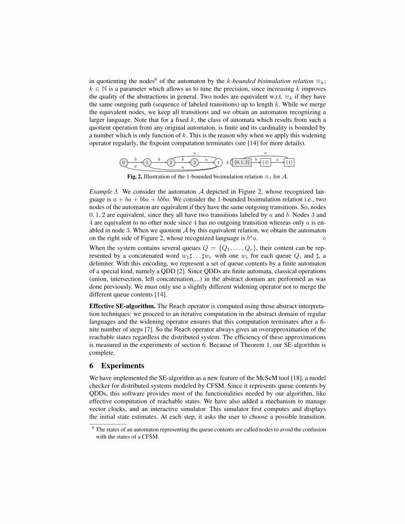
in quotienting the nodes6 of the automaton by the k-bounded bisimulation relation ≡k;k ∈ N is a parameter which allows us to tune the precision, since increasing k improvesthe quality of the abstractions in general. Two nodes are equivalent w.r.t. ≡k if they havethe same outgoing path (sequence of labeled transitions) up to length k. While we mergethe equivalent nodes, we keep all transitions and we obtain an automaton recognizing alarger language. Note that for a fixed k, the class of automata which results from such aquotient operation from any original automaton, is finite and its cardinality is bounded bya number which is only function of k. This is the reason why when we apply this wideningoperator regularly, the fixpoint computation terminates (see [14] for more details).

0 1 2 3 4b b b a

a

aa{0, 1, 2} {3} {4}b

b

a

a

Fig. 2. Illustration of the 1-bounded bisimulation relation ≡1 for A.

Example 3. We consider the automaton A depicted in Figure 2, whose recognized lan-guage is a + ba + bba + bbba. We consider the 1-bounded bisimulation relation i.e., twonodes of the automaton are equivalent if they have the same outgoing transitions. So, nodes0, 1, 2 are equivalent, since they all have two transitions labeled by a and b. Nodes 3 and4 are equivalent to no other node since 4 has no outgoing transition whereas only a is en-abled in node 3. When we quotient A by this equivalent relation, we obtain the automatonon the right side of Figure 2, whose recognized language is b∗a. �When the system contains several queues Q = {Q1, . . . , Qr}, their content can be rep-resented by a concatenated word w1] . . . ]wr with one wi for each queue Qi and ], adelimiter. With this encoding, we represent a set of queue contents by a finite automatonof a special kind, namely a QDD [2]. Since QDDs are finite automata, classical operations(union, intersection, left concatenation,...) in the abstract domain are performed as wasdone previously. We must only use a slightly different widening operator not to merge thedifferent queue contents [14].

Effective SE-algorithm. The Reach operator is computed using those abstract interpreta-tion techniques: we proceed to an iterative computation in the abstract domain of regularlanguages and the widening operator ensures that this computation terminates after a fi-nite number of steps [7]. So the Reach operator always gives an overapproximation of thereachable states regardless the distributed system. The efficiency of these approximationsis measured in the experiments of section 6. Because of Theorem 1, our SE-algorithm iscomplete.

6 ExperimentsWe have implemented the SE-algorithm as a new feature of the McScM tool [18], a modelchecker for distributed systems modeled by CFSM. Since it represents queue contents byQDDs, this software provides most of the functionalities needed by our algorithm, likeeffective computation of reachable states. We have also added a mechanism to managevector clocks, and an interactive simulator. This simulator first computes and displaysthe initial state estimates. At each step, it asks the user to choose a possible transition.

6 The states of an automaton representing the queue contents are called nodes to avoid the confusionwith the states of a CFSM.

If the chosen transition is an output, it attaches the current state estimate of the activesubsystem and its vector clock to the message sent, and updates the local state estimate. Ifthe transition is an input, the local estimator reads the information attached to the receivedmessage and updates its state estimate.

We proceeded to an evaluation of our algorithm measuring the size of the state esti-mates. Note that this size is not the number of global states of the state estimate (whichmay be infinite) but the number of nodes of its QDD representation. We generated randomsequences of transitions for our running example and some other examples of [12]. Table 1shows the average execution time for a random sequence of 100 transitions, the memoryrequired (heap size), the average and maximal size of the state estimates. Default valueof the widening parameter is k = 1. Experiments were done on a standard MacBook Prowith a 2.4 GHz Intel core 2 duo CPU.

example # subsystems # channels time [s] memory [MB] maximal size average sizerunning example 3 4 7.13 5.09 143 73.0c/d protocol 2 2 5.32 8.00 183 83.2non-regular protocol 2 1 0.99 2.19 172 47.4ABP 2 3 1.19 2.19 49 24.8sliding window 2 2 3.26 4.12 21 10.1POP3 2 2 3.08 4.12 22 8.5

Table 1. Experiments

These results show that the computation of state estimates takes about 50ms per transitionand that the symbolic representation of state estimates we add to messages are automatawith a few dozen nodes. A sensitive element in the method is the size of the computedand transmitted information. It can be improved by the use of compression techniques toreduce the size of this information. A more evolved technique would consist in the offlinecomputation of the set of possible estimates. Estimates are indexed in a table, availableat execution time to each local estimator. If we want to keep an online algorithm, wecan use the memoization technique. When a state estimate is computed for the first time,it is associated with an index that is transmitted to the subsystem which records bothvalues. If the same estimate must be transmitted, only its index can be transmitted and thereceiver can find from its table the corresponding estimate. Those techniques are not yetimplemented.

We also highlight that our method works better on the real-life communication proto-cols we have tested (alternating bit protocol, sliding window, POP3) than on the exampleswe introduced to test our tool. More details about the tool and experiments are given inAppendix B.

7 Conclusion and Future Work

We have proposed an effective algorithm to compute online, locally to each subsystem, anestimate of the global state of a running distributed system, modeled as communicatingfinite state machines with reliable unbounded FIFO queues. With such a system, a globalstate is composed of the current location of each subsystem together with the channelcontents. The principle is to add a local estimator to each subsystem such that most ofthe system is preserved; each local estimator is only able to compute information and

in particular symbolic representations of state estimates and to piggyback some of thiscomputed information to the transmitted messages. Since these estimates may be infinite,a crucial point of our work has been to propose and evaluate the use of regular languagesto abstract sets of FIFO queues. In practice, we have used k-bisimilarity relations, whichallows us to represent each (possibly infinite) set of queue contents by the minimal andcanonical k-bisimilar finite automaton which gives an overapproximation of this set. Ouralgorithm transmits state estimates and vector clocks between subsystems to allow them torefine and preserve consistent state estimates. More elaborate examples must be taken toanalyze the precision of our algorithm and see, in practice, if the estimates are sufficient tosolve diagnosis or control problems. Anyway, it appears important to study the possibilityof reducing the size of the added communication while preserving or even increasing theprecision in the transmitted state estimates.

References

1. G. Berry and G. Gonthier. The esterel synchronous programming language: Design, semantics,implementation. Sci. Comput. Program., 19(2):87–152, 1992.

2. B. Boigelot, P. Godefroid, B. Willems, and P. Wolper. The power of QDDs. In SAS ’97:Proceedings of the 4th International Symposium on Static Analysis, pages 172–186, 1997.

3. Ahmed Bouajjani and Peter Habermehl. Symbolic reachability analysis of fifo-channel systemswith nonregular sets of configurations. Theor. Comput. Sci., 221(1-2):211–250, 1999.

4. D. Brand and P. Zafiropulo. On communicating finite-state machines. J. ACM, 30(2):323–342,1983.

5. C. Cassandras and S. Lafortune. Introduction to Discrete Event Systems. Kluwer AcademicPublishers, 1999.

6. T. Chatain, P. Gastin, and N. Sznajder. Natural specifications yield decidability for distributedsynthesis of asynchronous systems. In SOFSEM, volume 5404 of LNCS, pages 141–152, 2009.

7. P. Cousot and R. Cousot. Abstract interpretation: a unified lattice model for static analysis ofprograms by construction or approximation of fixpoints. In POPL’77, pages 238–252, 1977.

8. R. Debouk, S. Lafortune, and D. Teneketzis. Coordinated decentralized protocols for failure di-agnosis of discrete event systems. Discrete Event Dynamical Systems: Theory and Applications,10:33–79, 2000.

9. Alain Finkel, S. Purushothaman Iyer, and Gregoire Sutre. Well-abstracted transition systems:application to fifo automata. Information and Computation, 181(1):1–31, 2003.

10. B. Genest. On implementation of global concurrent systems with local asynchronous con-trollers. In CONCUR, volume 3653 of LNCS, pages 443–457, 2005.

11. L. Helouet, T. Gazagnaire, and B. Genest. Diagnosis from scenarios. In proc. of the 8th Int.Workshop on Discrete Events Systems, WODES’06, pages 307–312, 2006.

12. A. Heußner, T. Le Gall, and G. Sutre. Extrapolation-Based Path Invariants for AbstractionRefinement of Fifo Systems. In Proc. Model Checking Software, SPIN Workshop 2009, volume5578 of LNCS, pages 107–124. Springer, 2009.

13. L. Lamport. Time, clocks, and the ordering of events in a distributed system. Communicationsof the ACM, 21(7):558–565, 1978.

14. T. Le Gall, B. Jeannet, and T. Jeron. Verification of communication protocols using abstractinterpretation of fifo queues. In AMAST ’06, volume 4019 of LNCS, July 2006.

15. F. Lin, K. Rudie, and S. Lafortune. Minimal communication for essential transitions in a dis-tributed discrete-event system. IEEE Trans. on Automatic Control, 52(8):1495–1502, 2007.

16. T. Massart. A calculus to define correct tranformations of lotos specifications. In FORTE,volume C-2 of IFIP Transactions, pages 281–296, 1991.

17. F. Mattern. Virtual time and global states of distributed systems. In Proceedings of the Workshopon Parallel and Distributed Algorithms, pages 215–226, 1989.

18. The McScM library, 2009. http://www.labri.fr/perso/heussner/mcscm/.19. L. Ricker and B. Caillaud. Mind the gap: Expanding communication options in decentralized

discrete-event control. In 46th IEEE Conference on Decision and Control, New Orleans, LA,USA, 2007.

20. M. Sampath, R. Sengupta, S. Lafortune, K. Sinaamohideen, and D. Teneketzis. Failure diagnosisusing discrete event models. IEEE Transactions on Control Systems Technology, 4(2):105–124,March 1996.

21. S. Tripakis. Decentralized control of discrete event systems with bounded or unbounded delaycommunication. IEEE Trans. on Automatic Control, 49(9):1489–1501, 2004.

22. S. Xu and R. Kumar. Distributed state estimation in discrete event systems. In ACC’09: Proc.of the 2009 conference on American Control Conference, pages 4735–4740, 2009.

A Proofs of Theorems 1 and 2

In this section, we prove Theorems 1 and 2. These proofs use the lemmas given in sec-tion A.1 and the following notations.

Let s = x0e1−→ x1

e2−→ . . .em−−→ xm be an execution of the global system T . When the

subsystem Ti executes an event ek (with k ∈ [1,m]) of this sequence, the state estimate,computed by Ei at this step, is denoted by Eti , where t is the number of events executedby Ti in the subsequence x0

e1−→ x1e2−→ . . .

ek−→ xk. However, to be more concise in ourpresentation, we use an abuse of notation: when an event ek is executed in the sequences, the state estimate of each state estimator Ei is denoted by7 Eki . This state estimate is

defined in the following way: if ek has not been executed by Ti, then Ekidef= Ek−1i .

Otherwise, the value of Eki is computed by the state estimator from Ek−1i , the observedevent, and the information that possibly tags this event.

The vector clock Vi, computed after the occurrence of an event e in the subsystem Ti,is denoted by Vi(e).

A.1 Lemmas

The following lemma proves the correctness of the vector clock mapping computed by theMattern’s algorithm for the relation ≺c:Lemma 1 ([17]). Given n subsystems Ti (∀i ∈ [1, n]) and two events e1 6= e2 occurringrespectively in Ti and Tj (i can be equal to j), we have the following equivalence: e1 ≺ce2 if and only if Vi(e1) ≤ Vj(e2).

Lemma 2. Given n subsystems Ti (∀i ∈ [1, n]) and three events ei 6= ej 6= ek occurringrespectively in Ti, Tj and Tk , if ek 6≺c ej and ei ≺c ej , then ek 6≺c ei.

Proof. Let us assume that ek ≺c ei. Since ek 6≺c ej , there exists ` ∈ [1, n] such thatVk(ek)[`] > Vj(ej)[`]. Moreover, Vk(ek)[`] > Vi(ei)[`], because Vi(ei)[m] ≤ Vj(ej)[m]for each m ∈ [1, n] (due to ei ≺c ej). But it is a contradiction with ek ≺c ei, because thisrelation implies that Vk(ek)[m] ≤ Vi(ei)[m] for each m ∈ [1, n]. �

7 In this way, we do not need to introduce, for each subsystem, a parameter giving the number ofevents that has been executed so far by each subsystem

Lemma 3. Given a distributed system T = T1|| . . . ||Tn , and a sequence se1 = x0e1−→

x1e2−→ . . .

ei−1−−−→ xi−1ei−→ xi

ei+1−−−→ xi+1ei+2−−−→ . . .

em−−→ xm executed by T , if ei 6≺c ei+1,then the sequence se2 = x0

e1−→ x1e2−→ . . .

ei−1−−−→ xi−1ei+1−−−→ x′i

ei−→ xi+1ei+2−−−→ . . .

em−−→xm can also occur in the system T .

Proof. We suppose that δei = 〈`ei , σei , `′ei〉 ∈ ∆i and δei+1 = 〈`ej , σej , `′ej 〉 ∈ ∆j . Notethat i 6= j; otherwise, we would have ei ≺c ei+1 (by definition of ≺c). We can provethis property by showing that PostTδei+1

(PostTδei(xi−1)) = PostTδei

(PostTδei+1(xi−1)). For

that, we consider two cases:1) δei and δei+1

act on different queues: we suppose that δei and δei+1respectively

act on the queues Qki and Qkj . We also suppose that xi−1 = 〈`1, . . . , `ei ,. . . , `ej ,. . . , `n, w1, . . . , wki , . . . , wkj , . . . , w|Q|〉 (where wki and wkj respectively denote thecontent of the queues Qki and Qkj ), and that the action σei (resp. σej ), which actson the content wki (resp. wkj ), modifies it to give w′ki (resp. w′kj ). In consequence,PostTδei

(xi−1) = 〈`1, . . . , `′ei ,. . . , `ej , . . . , `n, w1, . . . , w′ki, . . . , wkj , . . . , w|Q|〉

and PostTδei+1(PostTδei

(xi−1)) = 〈`1, . . . , `′ei ,. . . , `′ej , . . . , `n, w1, . . . , w′ki, . . . ,

w′kj , . . . , w|Q|〉. Since ei 6≺c ei+1, we have that PostTδei+1(xi−1) = 〈`1, . . . , `ei ,. . . ,

`′ej , . . . , `n, w1, . . . , wki , . . . , w′kj, . . . , w|Q|〉 and PostTδei

(PostTδei+1(xi−1)) =

〈`1, . . . , `′ei ,. . . , `′ej , . . . , `n, w1, . . . , w′ki, . . . , w′kj , . . . , w|Q|〉, which implies that

PostTδei+1(PostTδei

(xi−1)) = PostTδei(PostTδei+1

(xi−1)).

2) δei and δei+1 act on the same queue Qk: we consider two cases:a) σi = Qk!mi is an output and σi+1 = Qk?mj is an input: the message written

by δei cannot be read by the transition δei+1 , because, in this case, we would haveei ≺c ei+1. Thus, PostTδei+1

(PostTδei(xi−1)) = 〈`1, . . . , `′ei ,. . . , `′ej , . . . , `n, w1,

. . . , w.mi, . . . , w|Q|〉 where w.mi is the content of the queue Qk. Therefore, thestate PostTδei

(xi−1) = 〈`1, . . . , `′ei ,. . . , `ej , . . . , `n, w1, . . . , mj .w.mi, . . . , w|Q|〉and the state xi−1 = 〈`1, . . . , `ei ,. . . , `ej , . . . , `n, w1, . . . , mj .w, . . . , w|Q|〉.Next, we compute the state PostTδei+1

(xi−1) = 〈`1, . . . , `ei ,. . . , `′ej , . . . , `n, w1,

. . . , w, . . . , w|Q|〉 and the state PostTδei(PostTδei+1

(xi−1)) = 〈`1, . . . , `′ei ,. . . , `′ej ,. . . , `n, w1, . . . , w.mi, . . . , w|Q|〉. In consequence, PostTδei+1

(PostTδei(xi−1)) =

PostTδei(PostTδei+1

(xi−1)).

b) σi = Qk?mi is an input and σi+1 = Qk!mj is an output: the statePostTδei+1

(PostTδei(xi−1)) = 〈`1, . . . , `′ei ,. . . , `′ej , . . . , `n, w1, . . . , w.mj , . . . , w|Q|〉

where w.mj is the content of the queue Qk. Next, similarly to the previous case, wecan prove that PostTδei+1

(PostTδei(xi−1)) = PostTδei

(PostTδei+1(xi−1)).

The cases, where δei and δei+1are both an input or an output, are not possible, because

these transitions would then be executed by the same process and hence we would haveei ≺c ei+1. �

This property means that if two consecutive events ei and ei+1 are such that ei 6≺c ei+1,then these events can be swapped without modifying the reachability of xm. We finallyprove the following lemma.

Lemma 4. Given a distributed system T = T1|| . . . ||Tn , a transition δi =〈`i, Qt,i?mi, `

′i〉 ∈ ∆i (with t 6= i), and a set of states B ⊆ X , then

ReachT∆\∆i(PostTδei

(ReachT∆\∆i(B))) = PostTδei

(ReachT∆\∆i(B)).

Proof. First, the inequality PostTδei(ReachT∆\∆i

(B)) ⊆ReachT∆\∆i

(PostTδei(ReachT∆\∆i

(B))) holds trivially.To prove the other inclusion, we have to show that if a state xm ∈

ReachT∆\∆i(PostTδei

(ReachT∆\∆i(B))), then xm ∈ PostTδei

(ReachT∆\∆i(B)). We actually

prove a more general result. We show that each sequence x1e2−→ x2

e3−→ . . .ek−1−−−→

xk−1ek−→ xk

ek+1−−−→ xk+1ek+2−−−→ . . .

em−−→ xm (where (i) x1 ∈ B, (ii) the event ek cor-responds to the transition δek = δi ∈ ∆i, and (iii) the event eb, for each b 6= k ∈ [2,m],corresponds to a transition δeb ∈ ∆ \∆i) can be reordered to execute ek at the end of thesequence without modifying the reachability of xm i.e., the following sequence can occur:x1

e2−→ x2e3−→ . . .

ek−1−−−→ xk−1ek+1−−−→ x′k+1

ek+2−−−→ . . .em−−→ x′m

ek−→ xm. This reorderedsequence can be obtained thanks to Lemma 3, but to use this lemma, we must prove thatek 6≺c eb (∀b ∈ [k + 1,m]). The proof is by induction on the length of the sequence ofevents that begins from xk:

• Base case: we must prove that ek 6≺c ek+1. By definition of ≺c, since ek and ek+1

occur in different subsystems and are consecutive events, there is one possibility to haveek ≺c ek+1: it is when ek is an output and ek+1 is the corresponding input. But ek is aninput and hence ek 6≺c ek+1.

• Induction step: we suppose that ek 6≺c ek+r (∀r ∈ [1, j]) and we prove that ek 6≺cek+j+1. By definition of ≺c, since ek and ek+1 occur in different subsystems, there aretwo possibilities to have ek ≺c ek+j+1:

1) ek is an output and ek+j+1 is the corresponding input. However, ek is an input andthus this case is impossible.

2) ek ≺c ek+r (with r ∈ [1, j]) and ek+r ≺c ek+j+1. But by induction hypothesis,ek 6≺c ek+r (∀r ∈ [1, j]) and thus this case is impossible.

Therefore, ek 6≺c ek+j+1. �

A.2 Proof of Theorem 1

To show that this theorem holds, we prove by induction on the length m of an executionx0

e1−→ x1e2−→ . . .

em−−→ xm of the system T that ∀i ∈ [1, n] : ReachT∆\∆i(xm) ⊆ Emi .

Since xm ∈ ReachT∆\∆i(xm), we have then that xm ∈ Emi . In this proof, when ei ≺c ej ,

we say that ej causally depends on ei (or ei happened-before ej).

• Base case (m = 0): For each i ∈ [1, n], the set E0i =

ReachT∆\∆i(〈`0,1, . . . , `0,n, ε, . . . , ε〉) (see Algorithm 1). Therefore, we have that

ReachT∆\∆i(x0) = E0

i (∀i ∈ [1, n]), because x0 = 〈`0,1, . . . , `0,n, ε, . . . , ε〉.• Induction step: We suppose that the property holds for the executions of length k ≤ m

(i.e., ∀ 0 ≤ k ≤ m,∀i ∈ [1, n] : ReachT∆\∆i(xk) ⊆ Eki ) and we prove that the property

also holds for the executions of length m+ 1. For that, we suppose that the event em+1

has been executed by Ti. We must consider two cases:

1) δem+1is an output on the queue Qi,k (with k 6= i ∈ [1, n]): We must prove that

∀j ∈ [1, n] : ReachT∆\∆j(xm+1) ⊆ Em+1

j and we consider again two cases to provethis property:a) j 6= i: By induction hypothesis, we know that ReachT∆\∆j

(xm) ⊆ Emj . Moreover,we have that:

xm ⊆ ReachT∆\∆j(xm), by definition of Reach

⇒ PostTδem+1(xm) ⊆ PostTδem+1

(ReachT∆\∆j(xm)), as Post is monotonic

⇒ xm+1 ⊆ ReachT∆\∆j(xm), because δem+1

∈ ∆ \∆j (as δem+1∈ ∆i) and

PostTδem+1(xm) = xm+1

⇒ ReachT∆\∆j(xm+1) ⊆ ReachT∆\∆j

(ReachT∆\∆j(xm)), as Reach is monotonic

⇒ ReachT∆\∆j(xm+1) ⊆ ReachT∆\∆j

(xm)

⇒ ReachT∆\∆j(xm+1) ⊆ Emj

⇒ ReachT∆\∆j(xm+1) ⊆ Em+1

j , because Emj = Em+1j (due to the fact that

em+1 has not been executed by Tj)

b) j = i: By induction hypothesis, we know that ReachT∆\∆i(xm) ⊆ Emi . The set

Em+1i = ReachT∆\∆i

(PostTδem+1(Emi )) (see Algorithm 2). Moreover, we have that:

xm ⊆ ReachT∆\∆i(xm)

⇒ PostTδem+1(xm) ⊆ PostTδem+1

(ReachT∆\∆i(xm))

⇒ xm+1 ⊆ PostTδem+1(ReachT∆\∆i

(xm)), as PostTδem+1(xm) = xm+1

⇒ ReachT∆\∆i(xm+1) ⊆ ReachT∆\∆i

(PostTδem+1(ReachT∆\∆i

(xm)))

⇒ ReachT∆\∆i(xm+1) ⊆ ReachT∆\∆i

(PostTδem+1(Emi )), by induction hypothesis

⇒ ReachT∆\∆i(xm+1) ⊆ Em+1

i , by definition of Em+1i

Thus, for each j ∈ [1, n], we have that ReachT∆\∆j(xm+1) ⊆ Em+1

j . Moreover, sincewe compute an overapproximation ofEm+1

j (∀j ∈ [1, n]), this inclusion remains true8.

2) δem+1 is an input on the queue Qk,i (with k 6= i ∈ [1, n]): We must prove that ∀j ∈[1, n] : ReachT∆\∆j

(xm+1) ⊆ Em+1j and we consider again two cases:

a) j 6= i: The proof is similar to the one given in the case where δem+1 in an output.

b) j = i: By induction hypothesis, we know that ReachT∆\∆i(xm) ⊆ Emi . By Al-

gorithm 3, the set Em+1i = Temp1 ∩ PostTδem+1

(Emi ) (in our algorithm, the

set Temp1 can have three possible values). To prove that ReachT∆\∆i(xm+1) ⊆

Em+1i , we first prove that ReachT∆\∆i

(xm+1) ⊆ PostTδem+1(Emi ) and next we

show that ReachT∆\∆i(xm+1) ⊆ Temp1. The first inclusion is proved as follows:

8 Note that if we compute an underapproximation of Em+1j , the inclusion does not always hold.

xm ⊆ ReachT∆\∆i(xm)

⇒ PostTδem+1(xm) ⊆ PostTδem+1

(ReachT∆\∆i(xm))

⇒ xm+1 ⊆ PostTδem+1(ReachT∆\∆i

(xm)), because PostTδem+1(xm) = xm+1

⇒ ReachT∆\∆i(xm+1) ⊆ ReachT∆\∆i

(PostTδem+1(ReachT∆\∆i

(xm)))

⇒ ReachT∆\∆i(xm+1) ⊆ PostTδem+1

(ReachT∆\∆i(xm)), by Lemma 4

⇒ ReachT∆\∆i(xm+1) ⊆ PostTδem+1

(Emi ), by induction hypothesis

To prove the second inclusion, we must consider three cases which depend on thedefinition of Temp1. Let et (with t ≤ m) be the output (executed by Tk withk 6= i ∈ [1, n]) corresponding to the input em+1:

A) Temp1 = PostTδem+1(ReachT∆\∆i

(PostTδet (Et−1k ))) and Vk[i] = Vi[i] (as a

reminder, Vk represents the vector clock of Tk after the occurrence of the eventet and Vi represents the vector clock of Ti before the occurrence of the eventem+1): By induction hypothesis, we know that ReachT∆\∆k

(xt−1) ⊆ Et−1k .Moreover, we have that:

xt−1 ⊆ ReachT∆\∆k(xt−1)

⇒ xt−1 ⊆ Et−1k , by induction hypothesis

⇒ PostTδet (xt−1) ⊆ PostTδet (Et−1k )

⇒ xt ⊆ PostTδet (Et−1k ), as PostTδet (xt−1) = xt

⇒ ReachT∆\∆i(xt) ⊆ ReachT∆\∆i

(PostTδet (Et−1k )) (β)

However, since Vk[i] = Vi[i], we know that, between the moment where et hasbeen executed and the moment where em has been executed, the vector clockVi[i] has not been modified. Thus, during this period no transition of Ti hasbeen executed. In consequence, we have that xm ⊆ ReachT∆\∆i

(xt) and hencexm ⊆ ReachT∆\∆i

(PostTδet (Et−1k )) by (β). From this inclusion, we deduce

that:

PostTδem+1(xm) ⊆ PostTδem+1

(ReachT∆\∆i(PostTδet (E

t−1k )))

⇒ xm+1 ⊆ PostTδem+1(ReachT∆\∆i

(PostTδet (Et−1k ))),

because xm+1 = PostTδem+1(xm)

⇒ ReachT∆\∆i(xm+1) ⊆ ReachT∆\∆i

(PostTδem+1(ReachT∆\∆i

(PostTδet (Et−1k ))))

⇒ ReachT∆\∆i(xm+1) ⊆ PostTδem+1

(ReachT∆\∆i(PostTδet (E

t−1k ))),

by Lemma 4⇒ ReachT∆\∆i

(xm+1) ⊆ Temp1, by definition of Temp1

B) Temp1 = PostTδem+1(ReachT∆\∆i

(ReachT∆\∆k(PostTδet (E

t−1k )))) and Vk[k] >

Vi[k] (as a reminder, Vk represents the vector clock of Tk after the occurrenceof the event et and Vi represents the vector clock of Ti before the occurrence ofthe event em+1): By induction hypothesis, we know that ReachT∆\∆k

(xt−1) ⊆Et−1k . Moreover, we have that:

xt−1 ⊆ ReachT∆\∆k(xt−1)⇒ xt−1 ⊆ Et−1k , by induction hypothesis

⇒ PostTδet (xt−1) ⊆ PostTδet (Et−1k )

⇒ xt ⊆ PostTδet (Et−1k ), because PostTδet (xt−1) = xt (γ)

This inclusion is used further in the proof. Now, we prove that xm ⊆ReachT∆\∆i

(ReachT∆\∆k(xt)). For that, let us consider the subsequence se =

xtet+1−−−→ xt+1

et+2−−−→ . . .em−−→ xm of the execution x0

e1−→ x1e2−→ . . .

em−−→ xm.Let eK1 be the first event of the sequence se executed9 by Tk and sI =eI1 , . . . , eI` (with I1 < . . . < I`) be the events of the sequence se exe-cuted10 by Ti. If I` < K1 (i.e., eI` has been executed before eK1

), thenxm ⊆ ReachT∆\∆i

(ReachT∆\∆k(xt)), because all the events of the sequence

se executed by Ti have been executed before the first event eK1of Tk. Other-

wise, let sI′ = eId , . . . , eI` be the events of sI executed after eK1. We must

reorder the sequence se to obtain a new sequence where all the actions of Ti areexecuted before the ones of Tk and xm remains reachable. Lemma 3 allows usto swap two consecutive events without modifying the reachability when theseevents are not causally dependent. To use this lemma, we must prove that theevents eId , . . . , eI` do not causally depend on eK1

. For that, we first prove thateK1

6≺c eI` . By assumption, we know that Vk[k] > Vi[k]. Vk represents thevector clock of Tk after the execution of et and Vi represents the vector clockof Ti before the execution of em+1, which gives Vk(et)[k] > Vi(em)[k]. More-over, Vi(em)[k] ≥ Vi(eI`)[k] (because eI` has been executed before11 em) andVk(eK1

)[k] ≥ Vk(et)[k] + 1 (because eK1is the event which follows et in

the execution of the subsystem Tk). Thus, Vk(eK1)[k] > Vi(eI`)[k], and hence

eK1 6≺c eI` . Next, since eIc ≺c eI` (∀eIc 6= eI` ∈ sI′ ) and since eK1 6≺c eI` ,we have by Lemma 2 that eK1

6≺c eIc . Now, in the sequence se, we will movethe events eId , . . . , eI` to execute them before eK1

without modifying the reach-ability of xm. We start by moving the element eId . To obtain a sequence whereeId precedes eK1

, we swap eId with the events which precede it and we repeatthis operation until the event eK1

. Lemma 3 ensures that xm remains reachableif eId is swapped with an element e′ such that e′ 6≺c eId . However, betweeneK1

and eId there can be some events, that happened-before eId . We must thusmove these events before moving eId . More precisely, let sb = eb1 , . . . , ebp

9 If this element does not exist, then the transitions executed in this sequence do not belong to ∆k;thus, xm ⊆ ReachT∆\∆k

(xt) and hence xm ⊆ ReachT∆\∆i(ReachT∆\∆k

(xt))10 If the sequence sI is empty, then the transitions executed in the sequence se do not belong to∆i; thus, xm ⊆ ReachT∆\∆i

(xt) and hence xm ⊆ ReachT∆\∆i(ReachT∆\∆k

(xt)), becausext ⊆ ReachT∆\∆k

(xt)11 Note that eI` may be equal to em.

(with b1 < . . . < bp) be the greatest sequence of events such that (i) theseevents are executed between the occurrence of eK1

and the occurrence of eIdand (ii) ∀ebc ∈ sb : ebc ≺c eId (note that the events of the sequence sb are notexecuted by Tk; otherwise, we would have eK1

≺c eId ). The sequence of eventss = eK1

, eK1+1, eK1+2, . . . , eb1−1 executed between eK1and eb1 is such that

∀et′ ∈ s : et′ 6≺c eb1 . Indeed, if et′ ≺c eb1 , then by transitivity we wouldhave et′ ≺c eId , but this is not possible, because et′ 6∈ s. Thus, by Lemma 3,in the sequence xt

et+1−−−→ . . .eK1−−→ xK1

eK1+1−−−−→ xK1+1

eK1+2−−−−→ . . .eb1−1−−−→

xb1−1eb1−−→ xb1

eb1+1−−−→ . . .em−−→ xm, we can safely swap the events eb1−1 and

eb1 . We then obtain a reordered sequence where xm remains reachable i.e., weobtain xt

et+1−−−→ . . .eK1−−→ xK1

eK1+1−−−−→ xK1+1

eK1+2−−−−→ . . .eb1−2−−−→ xb1−2

eb1−−→x′b1

eb1−1−−−→ xb1eb1+1−−−→ . . .

em−−→ xm. By repeating this swap with the eventseb1−2, eb1−3, . . . , eK1+1, eK1 , we obtain a reordered sequence where (i) eb1 isexecuted before eK1

and (ii) xm remains reachable (by Lemma 3). We repeatthe operations performed for eb1 with the events eb2 , . . . , ebp and eId to ob-tain a reordered sequence where (i) eId is executed before eK1 and (ii) xm isreachable. Finally, we repeat the operations performed for eId with the otherelements of the sequence sI′ to obtain a reordered sequence where (i) xm isreachable from xt and (ii) the events of Ti are executed before the ones ofTk, which implies that xm ⊆ ReachT∆\∆i

(ReachT∆\∆k(xt)). Next, from this

inclusion, we deduce that:

PostTδem+1(xm) ⊆ PostTδem+1

(ReachT∆\∆i(ReachT∆\∆k

(xt)))

⇒ xm+1 ⊆ PostTδem+1(ReachT∆\∆i

(ReachT∆\∆k(xt))),

because xm+1 = PostTδem+1(xm)

⇒ ReachT∆\∆i(xm+1) ⊆ ReachT∆\∆i

(PostTδem+1(ReachT∆\∆i

(ReachT∆\∆k(xt))))

⇒ ReachT∆\∆i(xm+1) ⊆ PostTδem+1

(ReachT∆\∆i(ReachT∆\∆k

(xt))),

by Lemma 4⇒ ReachT∆\∆i

(xm+1) ⊆ PostTδem+1(ReachT∆\∆i

(ReachT∆\∆k(PostTδet (E

t−1k )))),

by (γ)

⇒ ReachT∆\∆i(xm+1) ⊆ Temp1, by definition of Temp1

C) Temp1 = PostTδem+1(ReachT∆(Post

Tδet

(Et−1k ))): By induction hypothesis, we

know that ReachT∆\∆k(xt−1) ⊆ Et−1k . Moreover, we have that:

xt−1 ⊆ ReachT∆\∆k(xt−1)⇒ xt−1 ⊆ Et−1k , by induction hypothesis

⇒ PostTδet (xt−1) ⊆ PostTδet (Et−1k )

⇒ xt ⊆ PostTδet (Et−1k ), as PostTδet (xt−1) = xt

⇒ ReachT∆(xt) ⊆ ReachT∆(PostTδet

(Et−1k )) (α)

However, the events et+1, . . . , em leading to xm from the state xt correspondto transitions which belong to ∆. Thus, xm ⊆ ReachT∆(xt) and hence xm ⊆ReachT∆(Post

Tδet

(Et−1k )) by (α). From this inclusion, we deduce that:

PostTδem+1(xm) ⊆ PostTδem+1

(ReachT∆(PostTδet

(Et−1k )))

⇒ xm+1 ⊆ PostTδem+1(ReachT∆(Post

Tδet

(Et−1k ))), as xm+1 =PostTδem+1(xm)

⇒ xm+1 ⊆ ReachT∆(PostTδet

(Et−1k )), because δem+1 ∈ ∆⇒ ReachT∆\∆i

(xm+1) ⊆ ReachT∆\∆i(ReachT∆(Post

Tδet

(Et−1k )))

⇒ ReachT∆\∆i(xm+1) ⊆ ReachT∆(Post

Tδet

(Et−1k )), because ∆ \∆i ⊆ ∆⇒ ReachT∆\∆i

(xm+1) ⊆ PostTδem+1(ReachT∆(Post

Tδet

(Et−1k ))),

because δem+1∈ ∆

⇒ ReachT∆\∆i(xm+1) ⊆ Temp1, by definition of Temp1

In conclusion, we have proven, for each definition of Temp1, thatReachT∆\∆i

(xm+1) ⊆ Temp1 and hence ReachT∆\∆i(xm+1) ⊆ Em+1

i .Thus, for each j ∈ [1, n], we have that ReachT∆\∆j

(xm+1) ⊆ Em+1j . Moreover, since

we compute an overapproximation of Em+1j (∀j ∈ [1, n]), this inclusion remains true.

A.3 Proof of Theorem 2To show that this theorem holds, we prove by induction on the length m of the sequencesof events e1, . . . , em (let δek = 〈`ek , σek , `′ek〉 be the transition corresponding to ek, foreach k ∈ [1,m]) executed by the system that ∀i ∈ [1, n] : Emi ⊆ {xr ∈ X|∃σ ∈P−1i (Pi(σe1 .σe2 . . . σem)) : x0

σ→ xr}:• Base case (m = 0): The initial state x0 = 〈`0,1, . . . , `0,n, ε, . . . , ε〉 and we must

prove that ∀i ∈ [1, n] : E0i ⊆ {xr ∈ X|∃σ ∈ P−1i (Pi(ε)) : x0

σ→ xr}. The set E0i =

ReachT∆\∆i(x0) (see Algorithm 1) and ReachT∆\∆i

(x0) = {xr ∈ X|∃σ ∈ P−1i (Pi(ε)) :

x0σ→ xr}, which implies that E0

i = {xr ∈ X|∃σ ∈ P−1i (Pi(ε)) : x0σ→ xr}.

Moreover, since we compute an underapproximation of E0i (∀j ∈ [1, n]), this inclusion

remains true12.• Induction step: We suppose that the property holds for the sequences of events of lengthk ≤ m and we prove that the property remains true for the sequences of length m + 1.We suppose that em+1 has been executed by Ti. We consider two cases:

1) δem+1is an output: We must prove that ∀j ∈ [1, n] : Em+1

j ⊆ {xr ∈ X|∃σ ∈P−1j (Pj(σe1 .σe2 . . . σem+1)) : x0

σ→ xr} and we consider again two cases:a) i 6= j: By induction hypothesis, we know that Emj ⊆ {xr ∈ X|∃σ ∈P−1j (Pj(σe1 .σe2 . . . σem)) : x0

σ→ xr}. Since Em+1j = Emj (by definition), we

have that Em+1j ⊆ {xr ∈ X|∃σ ∈ P−1j (Pj(σe1 .σe2 . . . σem)) : x0

σ→ xr}.12 Note that if we compute an overapproximation of the reachable states, the inclusion does not

always hold.

Moreover, {xr ∈ X|∃σ ∈ P−1j (Pj(σe1 .σe2 . . . σem)) : x0σ→ xr} = {xr ∈

X|∃σ ∈ P−1j (Pj(σe1 .σe2 . . . σem+1)) : x0

σ→ xr}, as Pj(σe1 .σe2 . . . σem) =

Pj(σe1 .σe2 . . . σem+1) (because σem+1

6∈ Σj). Therefore, we have that Em+1j ⊆

{xr ∈ X|∃σ ∈ P−1j (Pj(σe1 .σe2 . . . σem+1)) : x0σ→ xr}. Moreover, since we

compute an underapproximation of Em+1j , this inclusion remains true.

b) i = j: the set Em+1j = ReachT∆\∆j

(PostTδem+1(Emj )) and

Pj(σe1 .σe2 . . . σem+1) = Pj(σe1 .σe2 . . . σem).σem+1

, because σem+1∈ Σj . We

prove that if x ∈ Em+1j , then x ∈ {xr ∈ X|∃σ ∈ P−1j (Pj(σe1 .σe2 . . . σem+1)) :

x0σ→ xr}. If x ∈ Em+1

j , then there exists a state x′ ∈ Emjsuch that x ∈ ReachT∆\∆j

(PostTδem+1(x′)). Let 〈`em+1

, σem+1, `′em+1

〉,〈`t1 , σt1 , `′t1〉, . . . , 〈`tk , σtk , `′tk〉 be the sequence of transitions which leads to x

from x′ i.e., x′σem+1

.σt1...σtk−−−−−−−−−−→ x. The transition 〈`tb , σtb , `′tb〉 ∈ ∆\∆j (for each

b ∈ [1, k]), which implies that σem+1.σt1 . . . σtk ∈ P−1j (σem+1

). Moreover, byinduction hypothesis, the state x′ ∈ {xr ∈ X|∃σ ∈ P−1j (Pj(σe1 .σe2 . . . σem)) :

x0σ→ xr}, which implies that ∃σ′ ∈ P−1j (Pj(σe1 .σe2 . . . σem)) : x0

σ′→ x′.Since P−1j (Pj(σe1 .σe2 . . . σem+1

)) = [P−1j (Pj(σe1 .σe2 . . . σem)).P−1j (σem+1)],

the sequence σ′′ = σ′.σem+1.σt1 . . . σtk belongs to P−1j (Pj(σe1 .σe2 . . . σem+1

)).

Moreover, x0σ′′→ x (because x0

σ′→ x′ and x′σem+1

.σt1...σtk−−−−−−−−−−→ x) which implies

that x ∈ {xr ∈ X|∃σ ∈ P−1j (Pj(σe1 .σe2 . . . σem+1)) : x0

σ→ xr}. Hence,

Em+1j ⊆ {xr ∈ X|∃σ ∈ P−1j (Pj(σe1 .σe2 . . . σem+1

)) : x0σ→ xr}. Again, since

we compute an underapproximation of Em+1j , this inclusion remains true.

2) δem+1is an input: We must prove that ∀i ∈ [1, n] : Em+1

j ⊆ {xr ∈ X|∃σ ∈P−1j (Pj(σe1 .σe2 . . . σem+1

)) : x0σ→ xr} and we consider again two cases:

a) i 6= j: the proof is similar the one given in the case where δem+1is an output.

b) i = j: The set Em+1j = PostTδem+1

(Emj ) ∩ Temp1 (see Algorithm 3). Thus,

we have that Em+1j ⊆ PostTδem+1

(Emj ) and it then suffices to prove that

PostTδem+1(Emj ) ⊆ {xr ∈ X|∃σ ∈ P−1j (Pj(σe1 .σe2 . . . σem+1)) : x0

σ→ xr}.For that, we show that if x ∈ PostTδem+1

(Emj ), then x ∈ {xr ∈ X|∃σ ∈P−1j (Pj(σe1 .σe2 . . . σem+1

)) : x0σ→ xr}. If x ∈ PostTδem+1

(Emj ), then there

exists a state x′ ∈ Emj such that x = PostTδem+1(x′). By induction hypoth-

esis, the state x′ ∈ {xr ∈ X|∃σ ∈ P−1j (Pj(σe1 .σe2 . . . σem)) : x0σ→

xr}, which implies that ∃σ′ ∈ P−1j (Pj(σe1 .σe2 . . . σem)) : x0σ′→ x′. Since

P−1j (Pj(σe1 .σe2 . . . σem+1)) = [P−1j (Pj(σe1 .σe2 . . . σem)).P−1j (σem+1)], the se-

quence σ′′ = σ′.σem+1belongs to P−1j (Pj(σe1 .σe2 . . . σem+1

)). Moreover, x0σ′′→

x (because x0σ′→ x′ and x = PostTδem+1

(x′)) which implies that x ∈ {xr ∈X|∃σ ∈ P−1j (Pj(σe1 .σe2 . . . σem+1)) : x0

σ→ xr}. Therefore, we have that

Em+1j ⊆ {xr ∈ X|∃σ ∈ P−1j (Pj(σe1 .σe2 . . . σem+1

)) : x0σ→ xr}. Again, since

we compute an underapproximation of Em+1j , this inclusion remains true. �

B ExperimentsThis appendix presents some additional details about the current implementation of ouralgorithm. The source code is available: [18] version “0.02 Control”. Note that this tool isstill under development.

B.1 McScM tool - control versionMcScM [18] is a model checker for distributed systems modeled by CFSMs. It has beendeveloped by Alexander Heussner, Gregoire Sutre and Tristan Le Gall, and is distributedunder the LGPL license. We added, to this tool, an implementation of the state estimatealgorithm presented in this paper. McScM offers several model checking engines. Themodule we implemented is considered as a “new” engine. We call it by the command line:

mcscm.native -mc-engine control -simulation-only [otheroptions] <input>

The input is the model of the distributed system. The engine is called “control” because weaim at the control of distributed systems. By default, it starts with an interactive simulationof the model. At each step, the current state and the possible transitions are displayed. Theuser chooses one of these transitions and the tool updates the state of the system and thestate estimates according to our algorithm. By default, the state estimates are not displayed,but their size is displayed.

B.2 Experiment on the running exampleHere are some of the state estimates computed while the system executes the sequence ofactions of Example 2. The widening parameter is k = 1. Each estimate is a map froma global location to a queue content. We first give the initial estimate of each process.With the option -display-estimate, the tool displays, for each estimate and each location,the internal representation of the queue content - a QDD. We give here a more readablerepresentation as regular expression. We also give here the queue names as they appear inthe paper - the implementation uses numbers instead of names.

E1Location Q1,2 Q2,1 Q2,3 Q3,1

A0 ×B0 × C0 ε ε ε εE2

Location Q1,2 Q2,1 Q2,3 Q3,1

A0 ×B0 × C0 ε ε ε εA1 ×B0 × C0 c ε ε ε

E3Location Q1,2 Q2,1 Q2,3 Q3,1

A0 ×B0 × C0 ε ε ε εA1 ×B0 × C0 c ε ε εA1 ×B1 × C0 ε b∗ ε εA1 ×B2 × C0 ε b∗a+ ε ε εA1 ×B3 × C0 ε b∗a+ ε d ε

Location Q1,2 Q2,1 Q2,3 Q3,1

A1 ×B0 × C0 c ε ε εA1 ×B1 × C0 ε b∗ ε εA1 ×B2 × C0 ε b∗a ε εA1 ×B3 × C0 ε b∗a d εA1 ×B3 × C0 ε b∗a ε dA1 ×B3 × C1 ε b∗a ε ε

At the beginning, E1 knows exactly the current state,because nothing can happen if T1 does not sendmessage c to T2. E2 is almost as precise. HoweverE3 is less precise, because many events could occurbefore T3 receives its first message. After the firsttransition 〈A0, Q1,2!c, A1〉, the state estimate of theestimator E1 is similar to E3, but:

1. E1 does not know if T3 received d and sent another message d in channel Q3,1.2. the content of channel Q2,1 is a bit more precise, b∗a instead of b∗a + ε, because E1

knows that T1 did not receive any message.

Note that location A1×B3×C0 appears two times. The actual regular expression associ-ated to this location is ε#b∗a#(d#ε+ ε#d) where # is a special symbol to separate thedifferent queues. So we write it as ε#b∗a#d#ε+ ε#b∗a#ε#d in this state estimate.

If we continue, the tool calculates and displays the estimate as in Example 2. We onlygive, in the table below, the size of the estimates.

Subsystem Event E1 E2 E3− start 4 9 35T1 Q1,2!c 42 − −T2 Q1,2?c − 4 −T2 Q2,1!a − 9 −T2 Q2,3!d − 46 −T3 Q2,3?d − − 7T3 Q3,1!d − − 132T1 Q2,1?a 14 − −T1 Q3,1?d 4 − −