The University of MaineDigitalCommons@UMaine

Electronic Theses and Dissertations Fogler Library

Spring 5-10-2019

Global Performance Testing, Simulation, andOptimization of a 6-MW Annular FloatingOffshore Wind Turbine HullHannah L. AllenUniversity of Maine, hannah.louise.allen@maine.edu

Follow this and additional works at: https://digitalcommons.library.umaine.edu/etd

Part of the Ocean Engineering Commons

This Open-Access Thesis is brought to you for free and open access by DigitalCommons@UMaine. It has been accepted for inclusion in ElectronicTheses and Dissertations by an authorized administrator of DigitalCommons@UMaine. For more information, please contactum.library.technical.services@maine.edu.

Recommended CitationAllen, Hannah L., "Global Performance Testing, Simulation, and Optimization of a 6-MW Annular Floating Offshore Wind TurbineHull" (2019). Electronic Theses and Dissertations. 2959.https://digitalcommons.library.umaine.edu/etd/2959

GLOBAL PERFORMANCE TESTING, SIMULATION, AND OPTIMIZATION

OF A 6-MW ANNULAR FLOATING OFFSHORE WIND TURBINE HULL

By

Hannah Allen

B.S. University of New Haven, 2015

A THESIS

Submitted in Partial Fulfillment of the

Requirements for the Degree of

Master of Science

(in Mechanical Engineering)

May 2019

Advisory Committee:

Andrew J. Goupee, Assistant Professor of Mechanical Engineering, Co-Advisor

Habib J. Dagher, Director of the Advanced Structures and Composites Center,

Bath Iron Works Professor, Co-Advisor

Anthony M. Viselli, Research Assistant Professor and Manager of Offshore

Testing and Design, Advanced Structures and Composites Center

Masoud Rais-Rohani, Chair & Richard C. Hill Professor of Mechanical

Engineering

ii

© 2019 Hannah L. Allen

All Rights Reserved

GLOBAL PERFORMANCE TESTING, SIMULATION, AND OPTIMIZATION

OF A 6-MW ANNULAR FLOATING OFFSHORE WIND TURBINE HULL

By Hannah Allen

Thesis Co-Advisors: Dr. Andrew J. Goupee & Dr. Habib J. Dagher

An Abstract of the Thesis Presented

in Partial Fulfillment of the Requirements for the

Degree of Master of Science

(in Mechanical Engineering)

May 2019

Floating offshore wind turbine (FOWT) hull technologies are evolving rapidly

with many technically viable designs. However, a commercially dominant architecture

has yet to emerge. This thesis presents a methodology for evaluation of the hydrodynamic

performance of an annular FOWT hull. This hull shows significant promise from a

manufacturing and installation standpoint, but limited performance data exists. This

thesis will provide ample documentation on scale model testing of an annular FOWT hull

as well as the corresponding numerical validation approach and opportunities for design

improvement.

The first portion of this work involves testing a 1/100th-scale model in the Harold

Alfond Wind Wave Ocean Engineering Laboratory at the University of Maine’s

Advanced Structures and Composites Center followed by an investigation of wave-

induced motion using ANSYS AQWA, a commercial hydrodynamic software. The

experimental and numerical results are compared to determine the ability of ANSYS

AQWA to simulate the response of an annular FOWT hull, which here implies that the

hull contains a moonpool. The wave-only performance of the annular hull is also

compared to experimental data obtained for other baseline FOWT hulls. In addition to

quantifying a baseline hull this thesis will also explore modifications in the annular

geometry to further explore the design space in an effort to find a more optimal annular

hull configuration for use in FOWT applications.

iii

ACKNOWLEDGEMENTS

I would like to express my sincere gratitude to the generous contributions of the

Harold Alfond Foundation which provided the funding for this work. The Foundation’s

constant support of engineering feats and other areas in Maine does not go unnoticed.

It is difficult to generate a truly complete list of those who have helped me along

in this process. Certainly, thanks go out to the offshore team at the University of Maine’s

Advanced Structures and Composites Center including Chris Allen, Matt Cameron, and

Matt Fowler for their support of my model testing efforts as well as helping me navigate

the often choppy seas of learning the basics of floating offshore wind. Thank you also to

Lindsay Wells and Peter Jalbert for their constant camaraderie and help in model

fabrication and other areas. Thanks to the unsung heroes at the Composites Center behind

the scenes and out in the lab.

I cannot adequately express my gratitude to my advisor Dr. Andy Goupee for his

unwavering support of my learning process as he helped me to fearlessly apply myself to

this project without passing on shame for errors made along the way. Thank you to Dr.

Habib Dagher and Dr. Anthony Viselli for their continued passion for and support of

offshore wind in Maine —both for my own sake and for the sake of Maine’s future. I

would also like to thank Dr. Masoud Rais-Rohani for believing in me, perhaps more than

I have believed in myself at times. Without the dedication of these individuals, this work

would most certainly not have been possible.

It is important to me that the support from my family and friends does not go

unnoticed. Thanks to the numerous graduate students at the Composites Center among

them, in particular, Jacob Ward, William West, Rick Perry, Adam Letourneau, and

iv

Anthony Verzoni. Thank you to my parents Beth and Doug Allen for instilling in me the

belief that personal growth is always possible. Thank you to my brother Greg and my

sister Meredith for silently challenging me to push myself to keep up with their high

standards and determination. Finally, thank you to Kaitlyn Bartlett for her fierce belief

that I could make this a reality and for her ability to handle the crazy schedule and other

realities that have come with this quest.

v

TABLE OF CONTENTS

ACKNOWLEDGEMENTS ............................................................................................... iii

LIST OF TABLES ............................................................................................................. ix

LIST OF FIGURES ............................................................................................................ x

LIST OF NOMENCLATURE ......................................................................................... xiii

LIST OF ACRONYMS AND ABBREVIATIONS ......................................................... xv

CHAPTER 1 INTRODUCTION .........................................................................................1

1.1. Motivation .........................................................................................................1

1.2. Background .......................................................................................................2

1.2.1. Existing and in-the-Works Floating Offshore Wind Turbines ..........3

1.2.2. Use of Froude Scaling to Derive Equivalent 6-MW Systems .........11

1.2.3. Moonpools .......................................................................................15

1.3. Research Contributions ...................................................................................18

1.4. Thesis Overview .............................................................................................18

CHAPTER 2 EXPERIMENTAL COMPARISON OF AN ANNULAR

FLOATING OFFSHORE WIND TURBINE HULL AGAINST PAST MODEL

TEST DATA ......................................................................................................................20

2.1. Introduction .....................................................................................................20

2.2. Model Description ..........................................................................................21

2.3. Testing Environments .....................................................................................25

2.4. Numerical Modeling .......................................................................................26

2.5. Results .............................................................................................................29

vi

2.5.1. Position RAO Magnitudes ...............................................................30

2.5.1.1. Low-Energy Position RAO Magnitudes .......................... 30

2.5.1.2. High-Energy Position RAO Magnitudes ......................... 33

2.5.2. Nacelle Acceleration RAO Magnitudes ...........................................37

2.5.2.1. Low-Energy Nacelle Acceleration RAO Magnitudes ..... 37

2.5.2.2. High-Energy Nacelle Acceleration RAO Magnitudes ..... 39

2.5.3. Impacts of Heave Plate Addition .....................................................41

2.6. Discussion .......................................................................................................43

2.6.1. Comparison of Response in Low-Energy and High-Energy

Sea States ...................................................................................................44

2.6.2. Discrepancy between RAO Magnitudes Derived from

Irregular Waves and Regular Waves .........................................................45

2.6.3. ANSYS AQWA Modeling Capability .............................................45

2.6.4. Performance Comparison for Annular Hull and DeepCwind

Platforms ....................................................................................................45

2.6.5. Influence of Heave Plates on Performance ......................................46

CHAPTER 3 COMPARATIVE STUDY OF ANNULAR FOWT HULL

GEOMETRIES ..................................................................................................................47

3.1. Development of Hull Alternatives ..................................................................47

3.1.1. Shape Variations ..............................................................................47

3.1.2. Stability Requirements and Standardized Parameters .....................47

3.2. Shape Comparison Resulting Geometries ......................................................49

vii

3.3. ANSYS AQWA Parameters ...........................................................................51

3.3.1. Mesh Sizing .....................................................................................51

3.3.2. Modeling Parameters .......................................................................52

3.3.3. Assumptions and Simplifications ....................................................53

3.4. Results .............................................................................................................54

3.4.1. Natural Periods.................................................................................54

3.4.2. ANSYS AQWA Added Mass ..........................................................55

3.4.3. ANSYS AQWA Response Amplitude Operators ............................58

3.5. Discussion .......................................................................................................61

CHAPTER 4 SIZING OPTIMIZATION OF SQUARE ANNULAR HULL ...................63

4.1. Introduction .....................................................................................................63

4.2. Optimization Problem Statement ....................................................................63

4.2.1. Objective Functions .........................................................................64

4.2.2. Design Variables and Corresponding Bounds .................................65

4.2.3. Constraints .......................................................................................68

4.3. Use of NSGA-II Optimization Technique ......................................................69

4.4. Results .............................................................................................................72

4.5. Discussion .......................................................................................................76

CHAPTER 5 CONCLUSIONS AND FUTURE WORK ..................................................78

5.1. Conclusions .....................................................................................................78

5.2. Future Work ....................................................................................................79

REFERENCES ................................................................................................................. 81

APPENDIX A: Optimization MATLAB functions .......................................................... 86

viii

APPENDIX B: Optimization Generation 100 Population .............................................. 105

BIOGRAPHY OF THE AUTHOR ................................................................................. 108

ix

LIST OF TABLES

Table 1.1. Wind turbine scaling guidelines ...................................................................... 12

Table 1.2. 6-MW Froude Scaling information.................................................................. 12

Table 2.1. Select model specifications .............................................................................. 23

Table 2.2. Regular wave characteristics ........................................................................... 26

Table 2.3. Broadband wave characteristics ....................................................................... 26

Table 3.1. Shape variation standardized parameters ......................................................... 48

Table 3.2. Selected resulting parameters .......................................................................... 50

Table 3.3. Shape variation inertias and center of gravity locations .................................. 51

Table 3.4. Mesh characteristics ......................................................................................... 52

Table 3.5. Pitch and heave calculated natural periods ...................................................... 55

Table 4.1. Constant values ................................................................................................ 66

Table 4.2. Added mass coefficients .................................................................................. 67

Table 4.3. Geometric properties from selected Pareto Front individuals ......................... 75

Table B.1. Generation 100 Population ............................................................................ 105

x

LIST OF FIGURES

Figure 1.1 Orientations and degrees of freedom (Goupee et al., 2014) .............................. 3

Figure 1.2. Rendering of 6-MW Sea Reed (EOLFI, 2018) ................................................ 4

Figure 1.3. Rendering of Gusto MSC Tri-Floater (Huijs et al., 2014) ............................... 4

Figure 1.4. 2-MW WindFloat quayside (Principle, 2014) .................................................. 5

Figure 1.5. VolturnUS 1:8 scale quayside (Dagher et al., 2017) ........................................ 6

Figure 1.6. Fukushima Mirai installed (Kurtenbachap, 2013) ............................................ 6

Figure 1.7. Fukushima Shimpuu, fabrication complete (Mitsubishi

Corporation, 2015) ......................................................................................... 7

Figure 1.8. Fukushima Forward Hamakaze (Fukushima Offshore Wind

Consortium, 2016a)........................................................................................ 8

Figure 1.9. Statoil Hywind Scotland installation mockup (Equinor, 2018)........................ 8

Figure 1.10. Deployed Tetraspar (Lauridsen, 2017) ........................................................... 9

Figure 1.11. GICON-SOF installation mockup (GICON-SOF, 2015) ............................. 10

Figure 1.12. Floatgen installed (Ideol, 2018a) .................................................................. 11

Figure 1.13. Resulting geometries at 6-MW scale, part 1 ................................................ 13

Figure 1.14. Resulting geometries at 6-MW scale, part 2 ................................................ 14

Figure 1.15. Moonpool water motion during oscillation, calm water in transit

(Gaillarde & Cotteleer, 2005) ...................................................................... 17

Figure 2.1. 1/100th-scale model of annular hull floating wind turbine a) in the

process of trimming the hull and b) during testing ...................................... 21

Figure 2.2. Model dimensions .......................................................................................... 22

Figure 2.3. Basin layout .................................................................................................... 24

Figure 2.4. Mooring line surge restoring force ................................................................. 25

xi

Figure 2.5. Broadband wave spectrums from a) annular hull and b) DeepCwind

model test campaigns ................................................................................... 26

Figure 2.6. ANSYS AQWA mesh .................................................................................... 27

Figure 2.7. Overtopping during regular wave 4 ................................................................ 31

Figure 2.8. Low-energy surge position RAO magnitude comparison .............................. 32

Figure 2.9. Low-energy heave position RAO magnitude comparison ............................. 33

Figure 2.10. Low-energy pitch position RAO magnitude comparison ............................. 33

Figure 2.11. High-energy surge position RAO magnitude comparison ........................... 36

Figure 2.12. High-energy heave position RAO magnitude comparison ........................... 36

Figure 2.13. High-energy pitch position RAO magnitude comparison ............................ 37

Figure 2.14. Low-energy nacelle surge acceleration RAO magnitude comparison ......... 39

Figure 2.15. Low-energy nacelle heave acceleration RAO magnitude comparison ......... 39

Figure 2.16. High-energy nacelle surge acceleration RAO magnitude comparison ......... 41

Figure 2.17. High-energy nacelle heave acceleration RAO magnitude comparison ........ 41

Figure 2.18. ANSYS AQWA heave plate study: Heave RAO magnitude ....................... 43

Figure 2.19. ANSYS AQWA heave plate study: Pitch RAO magnitude ......................... 43

Figure 3.1. Standardized parameter visual ........................................................................ 49

Figure 3.2. Resulting footprints ........................................................................................ 50

Figure 3.3. Square annular hull with wave directions ...................................................... 52

Figure 3.4. Shape variation surge added mass .................................................................. 56

Figure 3.5. Shape variation heave added mass ................................................................. 57

Figure 3.6. Shape variation pitch added inertias ............................................................... 58

Figure 3.7. Shape variation surge RAOs .......................................................................... 58

xii

Figure 3.8. Shape variation heave RAOs .......................................................................... 60

Figure 3.9. Shape variation pitch RAOs ........................................................................... 61

Figure 4.1. Top-down and section view of hull ................................................................ 65

Figure 4.2. NSGA-II Generation 1 ................................................................................... 72

Figure 4.3. NSGA-II Generation 10 and Generation 50 ................................................... 73

Figure 4.4. NSGA-II Generation 100 ............................................................................... 74

xiii

LIST OF NOMENCLATURE

𝑏 = moonpool width

𝑐 = applied damping

𝑐𝑐𝑟 = critical damping

𝑑 = draft

𝑓1 = mass ratio

𝑓2 = pitch natural frequency ratio

𝑔 = gravitational constant

∬ 𝑥2𝑑𝐴 = area moment of inertia

𝐼𝑝𝑖𝑡𝑐ℎ = mass moment of inertia of system in pitch degree of freedom

𝐼𝑝𝑖𝑡𝑐ℎ 𝑎𝑑𝑑𝑒𝑑 = mass moment of inertia of added mass in pitch degree of freedom

𝐾𝑖 = waterplane stiffness for 𝑖𝑡ℎ degree of freedom

𝐾𝑝𝑖𝑡𝑐ℎ ℎ𝑦𝑑𝑟𝑜 = waterplane stiffness in pitch degree of freedom

𝐾𝑝𝑖𝑡𝑐ℎ 𝑚𝑜𝑜𝑟𝑖𝑛𝑔 = mooring stiffness in pitch degree of freedom

𝑙 = length of moonpool

𝑚ℎ𝑒𝑎𝑣𝑒 𝑎𝑑𝑑𝑒𝑑 = added mass in heave degree of freedom

𝑚𝑛𝑜𝑚 = nominal system mass

𝑚𝑡𝑜𝑡 = total system mass

𝑚𝑅𝑁𝐴 𝑜𝑟𝑖𝑔𝑖𝑛𝑎𝑙 = mass of original rotor-nacelle assembly

xiv

𝑚𝑅𝑁𝐴 6𝑀𝑊 = mass of 6MW rotor-nacelle assembly

𝜔𝑝𝑖𝑡𝑐ℎ 𝑛𝑜𝑚 = nominal pitch natural frequency

𝑃1 = moonpool width

𝑃2 = hull with

𝑃3 = heave plate width

𝑃4 = hull height

𝑡 = hull thickness

𝜃𝑝𝑖𝑡𝑐ℎ = rotation in pitch degree of freedom

𝑡𝑛𝑜𝑚𝑖𝑛𝑎𝑙 = nominal hull thickness

𝑇𝑛𝑝𝑖𝑡𝑐ℎ = system pitch natural period

𝑇𝑛𝑝𝑖𝑠𝑡𝑜𝑛 = moonpool piston natural period

𝑇𝑛𝑠𝑙𝑜𝑠ℎ𝑖𝑛𝑔 = moonpool sloshing natural period

𝑉 = submerged volume

𝑧𝑏 = vertical distance from waterline to center of buoyancy

𝑧𝑔 = vertical distance from waterline to center of gravity

𝜁 = damping ratio

xv

LIST OF ACRONYMS AND ABBREVIATIONS

AQWA = ANSYS AQWA

DOF = degrees of freedom

DNV = Det Norske Veritas

FOWT = floating offshore wind turbine

GA = genetic algorithm

GWh = gigawatt hour

kg = kilogram

km = kilometer

kN = kilonewton

m = meter

MWL = mean waterline

MW = megawatt

MWh = megawatt hour

NSGA-II = Non-dominated Sorting Genetic Algorithm-II

RNA = rotor-nacelle assembly

RAO = response amplitude operator

s = second

TLP = tension leg platform

1

CHAPTER 1

INTRODUCTION

1.1. Motivation

Floating offshore wind turbine (FOWT) hull technologies are evolving rapidly

with many technically viable designs. However, a commercially dominant architecture

has yet to emerge. Early hull designs including semisubmersible, spar, and tension leg

platforms (TLPs) were largely derived from offshore oil technologies but recent

developments in the commercial application and optimization of FOWTs have resulted in

a number of variations on these three varieties. The appeal of FOWT technology has

grown as projects such as Hywind Scotland and the University of Maine’s VolturnUS

have seen success and sustainable energy sources have become more desirable. FOWTs

also present noteworthy advantages over land and bottom-fixed turbines as they have

significant flexibility in where they can be placed and have a high potential to experience

consistent winds (Liu et al., 2016; Musial, 2018; Sclavounos, 2008). One example of this

is the United States where there is a large concentration of areas off the northeast and

west coasts with average wind speeds greater than 8 m/s (WINDExchange, 2017). In

addition to this, much of this wind is more economically accessible by FOWTs as a

majority of the offshore wind resources of the United States lies off the coasts of

California and New England in waters deeper than 60 m (Manzanas Ochagavia et al.,

2013; Musial et al., 2016).

Despite recent successes, resistance to FOWT projects continue largely due to

prohibitive cost. Costs for FOWTs are frequently driven by extensive electrical

infrastructure and the ocean conditions that must be accounted for in the support system

2

as compared to land-based systems. Per a 2017 report by Stehly et al., an average land-

based system cost $47/MWh as compared to $124/MWh for fixed-bottom wind. A

floating hull is required to use its geometry as well as an extensive mooring system to

minimize turbine motions without being directly rooted to the seafloor. As a result, the

per megawatt hour expenditures are even larger than for a fixed-bottom scenario totaling

an average of $146/MWh for FOWT systems (Stehly et al., 2017). Although the cost of

technology tends to decrease over time, there is still a significant cost associated with the

wind industry.

Unlike land-based wind turbines where foundations are responsible for a mere

4.0% of the project budget, the substructure and foundation for a floating system requires

29.5% of the budget (Stehly et al., 2017). Based on this it is easy to see at least one

opportunity for significant savings potential lies in optimizing the geometry of the hull.

Reduction in hull size and geometric complexity coupled with increased ease of

installation will play a pivotal role in helping the FOWT industry gain forward

momentum.

1.2. Background

There are a number of proposed and in-the-works designs for FOWT hulls, each

with the goal of surviving the marine environment while also managing to effectively

harvest wind energy. In an effort to understand the variety of concepts conceived to date,

a wide net was cast investigating commercially viable technologies. Each of the hull

technologies detailed in the following sections has its own methods for minimizing

platform and turbine motions in the heave, pitch, and surge degrees of freedom (DOF) as

3

illustrated in Figure 1.1, ranging from the deep drafts of spars to significant buoyancy of

semi-submersibles to large magnitudes of mooring tension for TLPs.

Figure 1.1 Orientations and degrees of freedom (Goupee et al., 2014)

Other hybrid concepts utilize combinations of these characteristics to achieve platform

stability. All of the numerous variations that have been developed aim to create a hull

which maximizes wind power harnessing potential by minimizing wind turbine motions

while keeping cost and other factors in mind. There is a wide variety of existing

technologies, but at the end of the exploratory phase, one promising design will be

selected for further testing and analysis in the remainder of this thesis.

1.2.1. Existing and in-the-Works Floating Offshore Wind Turbines

The DCNS Sea Reed (Figure 1.2) is a semi-submersible floater that is the result of

a collaborative effort between Alstom (now part of GE) and DCNS Marine Energy (now

Naval Energies). The Sea Reed hull is designed to support a 6-MW turbine with a hub

height (from the waterline to the nacelle) of approximately 100 m and a floater height

(from the bottom of the floater to base of the turbine tower) of 35 m. The design was

approved by the Bureau Veritas in June of 2017 and installation of four of these hulls is

intended to take place part way between Groix and Belle-Ile off the north-western coast

of France in 2020 (EOLFI, 2018).

4

Figure 1.2. Rendering of 6-MW Sea Reed (EOLFI, 2018)

Another triangular semi-submersible concept comes from Gusto MSC. The Gusto

MSC Tri-Floater is designed to support a 5-MW turbine at a hub height of 90 m with a

draft of 13.2 m (Huijs et al., 2014). The base of each of the three pillars features a heave

plate around the perimeter in an attempt to mitigate certain platform motions. The

mooring lines are mounted high above the mean water line (MWL) to reduce the

overturning moment which is caused by the interaction with the wind; this arrangement is

said to permit the use of a smaller floater. Unlike some other floaters, the Tri-Floater does

not rely on any active ballasting (GustoMSC, 2019).

Figure 1.3. Rendering of Gusto MSC Tri-Floater (Huijs et al., 2014)

Principle Power’s offshore turbine WindFloat (Figure 1.4) also uses a triangular

configuration. In this case, the connections between the columns are cylindrical members

5

which form a truss-like structure. Each of the vertical columns has a heave plate at the

bottom. This semi-submersible steel design was used for a 2-MW turbine located off the

coast of Portugal which produced over 17GWh of power in a test from 2011-2016. Three

8-MW iterations of this technology are intended to be deployed of the coast of Portugal

with funding granted in 2018 (Energias de Portugal, 2018). The WindFloat hull is also

intended to be used in a number of other projects globally in the coming years.

Figure 1.4. 2-MW WindFloat quayside (Principle, 2014)

An additional floater in the semisubmersible category is the 1:8 scale VolturnUS

floater which was deployed off Castine, Maine for 18 months starting in June of 2013.

This floater is a triangular semi-submersible. The floater supports a 12-kW wind turbine.

At 1:8 scale, the hull has a draft of 2.9 m and a hub height of 12.2 m. The test site

featured a water depth of 15 to 27 m. At full scale, this project is intended to support a 6-

MW turbine at a water depth of approximately 100 m (Dagher et al., 2017).

6

Figure 1.5. VolturnUS 1:8 scale quayside (Dagher et al., 2017)

Following the Fukushima nuclear disaster of 2011 Japan set out to explore

alternative energy sources. As a result of this exploration Japan pursued the potential of

floating offshore wind with three FOWT hull designs as part of the Fukushima Forward

project. Mirai, the four-column semi-submersible of this project is made from advanced

steel and supports a 2-MW downwind wind turbine. It is moored at a depth of 200 m.

This hull has a triangular configuration consisting of four columns with the central

column supporting the turbine. An active ballast system helps to minimize the floater

motions (Fukushima Offshore Wind Consortium, 2013). Funding for the project is

provided by Japan’s Ministry of Economy, Trade and Industry (offshoreWIND.biz,

2016a).

Figure 1.6. Fukushima Mirai installed (Kurtenbachap, 2013)

7

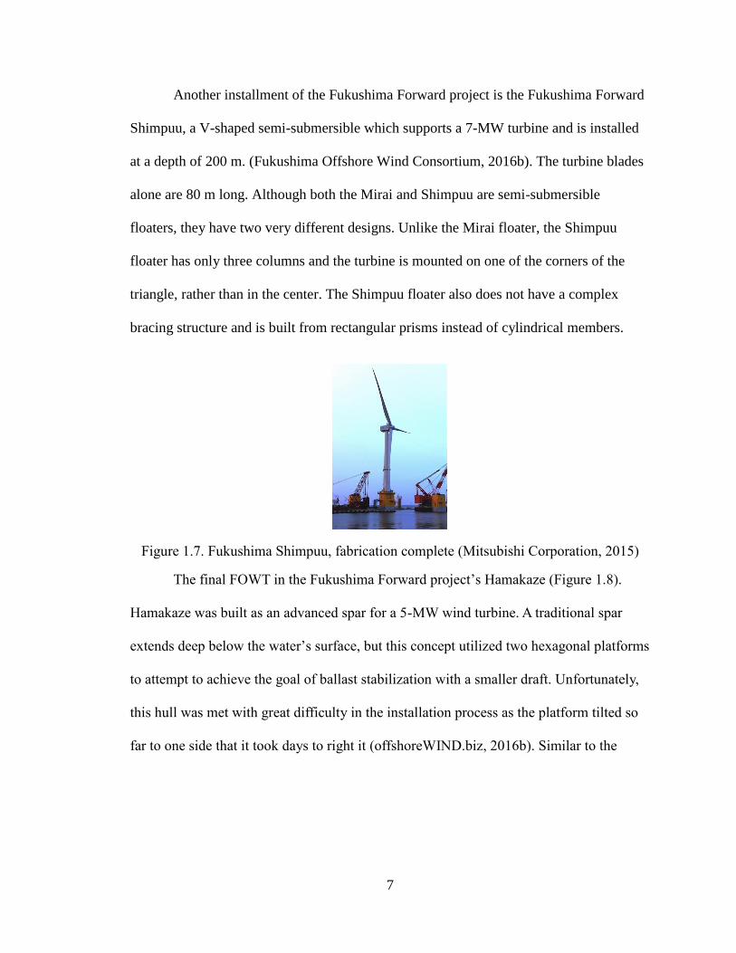
Another installment of the Fukushima Forward project is the Fukushima Forward

Shimpuu, a V-shaped semi-submersible which supports a 7-MW turbine and is installed

at a depth of 200 m. (Fukushima Offshore Wind Consortium, 2016b). The turbine blades

alone are 80 m long. Although both the Mirai and Shimpuu are semi-submersible

floaters, they have two very different designs. Unlike the Mirai floater, the Shimpuu

floater has only three columns and the turbine is mounted on one of the corners of the

triangle, rather than in the center. The Shimpuu floater also does not have a complex

bracing structure and is built from rectangular prisms instead of cylindrical members.

Figure 1.7. Fukushima Shimpuu, fabrication complete (Mitsubishi Corporation, 2015)

The final FOWT in the Fukushima Forward project’s Hamakaze (Figure 1.8).

Hamakaze was built as an advanced spar for a 5-MW wind turbine. A traditional spar

extends deep below the water’s surface, but this concept utilized two hexagonal platforms

to attempt to achieve the goal of ballast stabilization with a smaller draft. Unfortunately,

this hull was met with great difficulty in the installation process as the platform tilted so

far to one side that it took days to right it (offshoreWIND.biz, 2016b). Similar to the

8

other two FOWTs in the project, Hamakaze was moored at a depth of approximately 200

m (Fukushima Offshore Wind Consortium, 2013).

Figure 1.8. Fukushima Forward Hamakaze (Fukushima Offshore Wind Consortium,

2016a)

Statoil’s Hywind Scotland (Figure 1.9) takes a more traditional approach to the

spar with a cylindrical hull featuring a deep draft to utilize the stabilization from the low

center of gravity provided by the ballast. After testing a near commercial-scale prototype

with a 2.3-MW turbine off the coast of Norway—which saw winds of up to 40 m/s and a

maximum wave height of 19 m—a demonstration farm with full-scale turbines was

deployed in Scotland and started providing power to the grid in October of 2017. The full

scale deployment features five 6-MW turbines moored at water depths of 95 to129 m and

is the world’s first floating wind farms (Equinor, 2018).

Figure 1.9. Statoil Hywind Scotland installation mockup (Equinor, 2018)

The concept of Tetraspar was released in 2015 by Henrik Stiesdal. Unlike the

preceding hulls, the details of Tetraspar were fully released to the public. The intent of

9

this release was to enable any interested parties to push the development of this idea

forward. Tetraspar was designed to be a low-cost system with easy tow out and the ability

to be installed in water depths ranging from 10 m to 1000 m (Dvorak, 2015). The original

concept utilizes air-filled canisters at the bottom of the hull to provide flotation. The

Tetraspar can be deployed as a TLP with an anchor or a spar with a hanging mass as

shown in Figure 1.10.

Figure 1.10. Deployed Tetraspar (Lauridsen, 2017)

One example of a more traditional approach to the TLP is the TLP utilized by

GICON-SOF. As is typical of a TLP, the GICON-SOF is moored with taught vertical

mooring lines. The lines are attached to a large mass that sits on the sea floor as shown in

Figure 1.11. In this case, the hull is made from high performance prestressed concrete

and is intended to float out on top of a barge. The purpose of the barge is two-fold as it is

intended to be ballasted once it arrives at the installation site and lowered from the keel to

be used as the anchor for the system (GICON-SOF, 2018). The GICON-SOF concept is

still in development, but has been tested at a 1/37th scale in wind and waves at Maritime

10

Research Institute Netherlands. Supporting a 2.3-MW turbine would require that the

outer footprint of the floater measure 32 m by 32 m (Großmann et al., 2014).

Figure 1.11. GICON-SOF installation mockup (GICON-SOF, 2015)

The Ideol floating foundation does not resemble any of the aforementioned oil

and gas-style floating foundation examples. This hull is somewhat of a combination of a

barge and a typical semi-submersible hull. The item of greatest interest in this design is

the use of a moonpool (a material void) which is centrally located on the waterplane area.

The intended purpose of the moonpool is to use the water within it to counteract the

motion of the waters on the exterior of the hull. The hull geometry enables simpler

construction techniques and the low draft permits quayside turbine erection in a large

number of ports, eliminating costly turbine erection operations at sea. In addition, the

annular hull arrangement is stable during tow-out and only requires low-cost vessels for

installation.

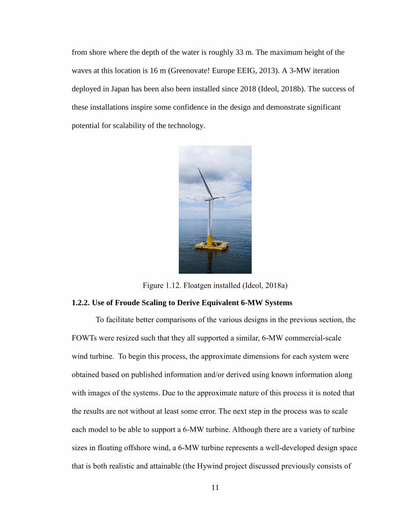
A 2-MW version of this design has been deployed in France and was

commissioned in 2018 (Ideol, 2018c). The assembly is located approximately 22 km

11

from shore where the depth of the water is roughly 33 m. The maximum height of the

waves at this location is 16 m (Greenovate! Europe EEIG, 2013). A 3-MW iteration

deployed in Japan has been also been installed since 2018 (Ideol, 2018b). The success of

these installations inspire some confidence in the design and demonstrate significant

potential for scalability of the technology.

Figure 1.12. Floatgen installed (Ideol, 2018a)

1.2.2. Use of Froude Scaling to Derive Equivalent 6-MW Systems

To facilitate better comparisons of the various designs in the previous section, the

FOWTs were resized such that they all supported a similar, 6-MW commercial-scale

wind turbine. To begin this process, the approximate dimensions for each system were

obtained based on published information and/or derived using known information along

with images of the systems. Due to the approximate nature of this process it is noted that

the results are not without at least some error. The next step in the process was to scale

each model to be able to support a 6-MW turbine. Although there are a variety of turbine

sizes in floating offshore wind, a 6-MW turbine represents a well-developed design space

that is both realistic and attainable (the Hywind project discussed previously consists of

12

five turbines of this size). The turbine was assumed to be installed at a hub height of 100

m with a rotor diameter of 150 m. The process of scaling these hulls was completed using

Froude Scaling (Chakrabarti, 1994). The scaling factor, 𝜆, employed in the Froude

scaling process was calculated by taking the cube root of the ratio of the mass of the

rotor nacelle assembly (RNA) for the baseline turbine for each system as compared to the

RNA of a standard 6-MW wind turbine as illustrated in ( 1.1 ).

𝜆3 =𝑚𝑅𝑁𝐴 𝑜𝑟𝑖𝑔𝑖𝑛𝑎𝑙

𝑚𝑅𝑁𝐴 6𝑀𝑊=

𝑚𝑅𝑁𝐴 𝑜𝑟𝑖𝑔𝑖𝑛𝑎𝑙

450𝑡 ( 1.1 )

Where: 𝑚𝑅𝑁𝐴 𝑜𝑟𝑖𝑔𝑖𝑛𝑎𝑙 is the mass of the original RNA

𝑚𝑅𝑁𝐴 6𝑀𝑊 is the mass of the 6-MW RNA

Relevant scale factor information is provided in Table 1.1. The original turbine sizes and

scaling factor for each hull are specified in Table 1.2. Resulting geometries for the

support of 6-MW turbines are shown in Figure 1.13 and Figure 1.14.

Table 1.1. Wind turbine scaling guidelines

Parameter Scale Factor

Length 𝜆

Volume 𝜆3

Mass 𝜆3

Table 1.2. 6-MW Froude Scaling information

FOWT Name Baseline Turbine

Size (MW)

Baseline Turbine

Mass (mt) Scale Factor

DCNS Sea Reed 6 450 1.000

Fukushima Forward Mirai 2 100 1.615

GustoMSC Tri-Floater 5 350 1.078

Principle Power WindFloat 2 100 1.615

GICON-SOF 2.3 150 1.456

Fukushima Forward Shimpuu 7 500 0.960

Ideol 2 100 1.546

Fukushima Forward Hamakaze 5 350 1.078

Statoil Hywind 6 350 1.068

Tetraspar 6 450 1.000

VolturnUS 6 450 1.000

13

Figure 1.13. Resulting geometries at 6-MW scale, part 1

14

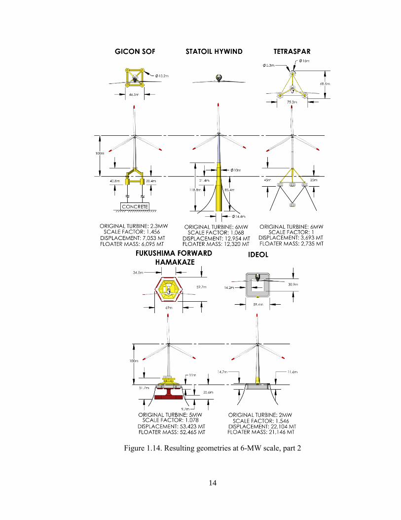
Figure 1.14. Resulting geometries at 6-MW scale, part 2

15

With each hull scaled to support a 6-MW wind turbine the geometries of the

systems were compared. Specific attention was paid to the footprint, draft, and any

unique qualities. A significant majority of the systems reviewed are semisubmersible tri-

floaters. Although this seems to indicate the significant potential for success of this

category, it also does not leave very much room for variability. The Hamakaze hull

exhibited significant issues in installation and a more traditional spar does not allow for

flexibility for affordable quayside turbine installation. Considering these factors as well

as the scarcity of publicly available global performance test data for floating hulls with

large moonpools relative to the size of the hull, the Ideol model was selected for further

studies. In order to best quantify the potential of such a design, there is significant interest

in understanding the dynamic performance of the moonpool of this hull and how it

impacts the system motions through both experimental and computational means.

1.2.3. Moonpools

The main focus of this thesis is on the data generation, model validation, and

optimization of a hull with a moonpool that is capable of supporting a 6-MW turbine. A

moonpool is a material void (shaft) which allows for water movement under and/or

within a hull or other floating body. Moonpools are widely used as a method of accessing

the subsea area with reduced impacts from exterior horizontal and vertical water motions

(Gaillarde & Cotteleer, 2005). The damping benefits involved in the applications of

moonpools are considered in three parts: potential/radiation damping, friction damping,

and viscous damping. The radiation damping is provided by outgoing waves that are the

result of the motion of the body and it is considered relatively small. There is some

damping which results from the friction of the water moving along the inner surface of

16

the moonpool, but this damping is considered to be negligible (Aalbers, 1984). This

leaves the viscous pressure damping as the most impactful form of damping resulting

from the moonpool.

Viscous damping is caused by vortex shedding due to vertical piston motion

within the moonpool which starts as the motion of the water in the moonpool nears its

piston natural frequency (see ( 1.2 )) (Gaillarde & Cotteleer, 2005). As the water within

the moonpool moves in the vertical direction, the downward motion of the water coupled

with the sharp edges at the base of the moonpool causes vortices to shed and a downward

forcing on the hull results in an increase in heave damping (Aalbers, 1984; Beyer et al.,

2015).

𝑇𝑛 𝑝𝑖𝑠𝑡𝑜𝑛 = 2𝜋√𝑑 + 0.41√𝑏𝑙

𝑔 ( 1.2 )

Where: 𝑑 is the draft of the hull

𝑏 is the width of the moonpool*

𝑙 is the length of the moonpool*

𝑔 in the gravitational constant *the product of 𝑏𝑙 was approximated as the

surface area of the pool for the triangular

and circular hulls discussed later

While the piston motion inside the moonpool represents the vertical motion of the

water, sloshing describes the primarily horizontal motion within the moonpool which is

caused by surge and sway motion from the structure. In the case of a moonpool in transit

in calm water illustrated in Figure 1.15, the sloshing motion occurs at the surface of the

moonpool, starting at one edge of the pool and moving to the opposite edge.

17

Figure 1.15. Moonpool water motion during oscillation, calm water in transit (Gaillarde

& Cotteleer, 2005)

As the motion begins to reflect back from the right edge of the moonpool to the starting

edge as shown in part c, the new wave that is forming on the left and moving to the right

begins to move to the right. When these two waves meet, there is a cancelling effect in

the motion of the water (Gaillarde & Cotteleer, 2005). This motion is initiated by water

motions outside the pool, but it also serves to at least partially counteract them. When it

comes to the offshore environment this represents a simplified case as there would be

waves coming from multiple directions with varying frequencies, but the principles are

likely to be very similar. The sloshing motion in a moonpool most prominent at the

sloshing natural period according to ( 1.3 ) (Molin, 2001).

𝑇𝑛𝑠𝑙𝑜𝑠ℎ𝑖𝑛𝑔= 2𝜋 √𝑔

𝜋

𝑏coth (

𝜋𝑑

𝑏+ 1.030) ( 1.3 )

Where: 𝑔 is the gravitational constant

𝑏 is the width of the moonpool

𝑑 is the draft of the hull

18

1.3. Research Contributions

The following academic contributions made by this thesis are as follows:

A review of experimental and numerical modeling methodologies including

modeling parameters and response amplitude operator (RAO) results to enable

replication of testing.

Capturing the impacts of moonpools on FOWT global performance in

numerical modeling including tuning of lid characteristics.

Assessment of FOWT global performance impacts resulting from moonpool

shape variation.

A study of quantifying the geometric tradeoffs of annular hulls when

optimizing mass and pitch natural frequency

1.4. Thesis Overview

Chapter 2 will describe the scale model testing parameters and the application of

Froude scaling to size the selected hull to model scale. Following this, the numerical

model validation process will be described. This description will include mesh and other

settings utilized in ANSYS AQWA (AQWA). AQWA is a hydrodynamic software that

uses a panel code to generate a potential flow solution to facilitate analysis in the time

domain as well as the frequency domain (ANSYS Inc., 2013a). For the purposes of this

work the Hydrodynamic Diffraction and Hydrodynamic Response analysis systems were

used to generate results in the frequency domain utilizing only the geometry at or below

the mean water line. Results comparisons between the scaled experimental model and

numerical model will also be reviewed.

19

In Chapter 3 numerical models of three alternative annular hull geometries will be

compared along with one barge model. Specified properties will be held constant across

all geometries while the dimensions of the waterplane area of the hulls will be permitted

to vary. The alternative geometries will be quantitatively evaluated for their linear static

stability, added mass/inertia and natural frequencies in surge, heave, and pitch DOF. In

addition, other factors such as cost will be discussed.

The contents of Chapter 4 revolve around the optimization of the hull geometry

selected in Chapter 3. The optimization process will explore the range of designs that

result from optimizing hull performance in platform pitch motion and system mass

simultaneously. While these features are optimized the draft, outer perimeter, and other

properties are permitted to vary. Unlike the hull resulting from Chapter 3 the optimized

hull is permitted to feature heave plates as an additional variation.

Conclusions and future work will be covered in Chapter 5. Final thoughts on the

numerical modeling process in regards to recommendations for and a review of methods

for appropriately modeling moored models with moonpools will be provided. The

geometric comparison results will then be revisited including a review of considered

parameters. Optimization of the square annular hull will also be discussed in Chapter 5.

The chapter will close with a discussion of areas which are recommended for further

investigation.

20

CHAPTER 2

EXPERIMENTAL COMPARISON OF AN ANNULAR FLOATING OFFSHORE

WIND TURBINE HULL AGAINST PAST MODEL TEST DATA

2.1. Introduction

With the annular 6-MW system selected, this chapter takes a closer look at the

performance of the system at model scale and attempts to reproduce those results with

numerical modeling. Although the intent of this study is to determine how an annular

hull-based system could behave, it is important to note that the system herein is

considered a generic system and is similar but not an exact reproduction of other annular

hulls proposed by Ideol and others.

Experimental modeling was completed for a generic 6-MW annular hull FOWT at

1/100th-scale in the University of Maine’s Harold Alfond Wind Wave (W2) Ocean

Engineering Laboratory in 2018. Although testing was carried out at model scale, all

data reported in this chapter is presented at full scale. The hydrodynamic performance of

the same FOWT was also modeled using AQWA. Comparison of experimental and

simulation RAO magnitudes for key positions and accelerations are conducted in an

effort to validate the AQWA simulations. RAO magnitudes represent the normalized

motion response of the system per unit wave amplitude input for a given wave frequency.

The experimental and simulation results for the annular FOWT hull are also compared to

a large model test data set obtained for the 5-MW DeepCwind semisubmersible, spar and

TLP for the purposes of putting the annular hull hydrodynamic performance in context

(Goupee et al., 2014; Koo et al., 2014). This past publically available data set has been

used extensively for numerical validation and represents reasonable performance of the

traditional floating hull design types (Hermans et al., 2016; Robertson & Jonkman, 2011).

21

2.2. Model Description

Both the experimental and numerical modeling completed considers a hull sized

to support a 6-MW turbine with a hub height of 100 m above the MWL. The models used

an equivalent point mass in place of a turbine and take only wave forcing into account.

Prior results (e.g. see (Goupee et al., 2014)) have shown that the linear wave response of

a FOWT’s dynamics are only weakly influenced by wind turbine forcing in the range of

periods considered, and as such, it is neglected here for simplicity (Coulling et al., 2013).

That noted, the annular hull geometry considered is generic with a square outer perimeter

and moonpool opening, as shown in Figure 2.1.

Figure 2.1. 1/100th-scale model of annular hull floating wind turbine a) in the process of

trimming the hull and b) during testing

All dimensions were approximated for a 2-MW system based on publicly

available data (LHEEA Centrale Nantes, 2018) and scaled to accommodate a 6-MW

turbine using Froude scaling (Det Norske Veritas, 2014). The Froude scaling was

(a) (b)

Qualysis markers

22

completed based on the scale factor resulting from the cube root of the ratio of the mass

of the 6-MW turbine as compared to the mass of the 2-MW turbine. The scale factor

obtained was 1.546. With the exception of the hub height, each length dimension from

the 2-MW system was scaled to the 6-MW system by multiplying the dimension by the

scaling factor. Additional system properties were calculated using the scaling factor and

Froude-scaling rules accordingly. The geometry of the tested annular hull, including the

local coordinate system used in this work, is given in Figure 2.2.

Figure 2.2. Model dimensions

The resulting gross properties of the 6-MW-sized hull are given in Table 2.1. Surge,

heave and pitch natural periods specified are obtained from free-decay testing. In the case

of heave, two harmonics were observed in the free-decay results with similar periods,

with the stronger of the two being 8.1 s. The weaker value harmonic exhibited a period of

approximately 10 s. The heave free-decay test results indicate a significant coupling

between the moonpool piston natural period and the heave natural period. Calculations

for the heave natural period of the system yield an expected value of 10.1 s.

23

Table 2.1. Select model specifications

Specification (units) Specified Value As-Built % Difference

Total System Mass (mt) 21,341 20,880 2.18

Displacement (mt) 21,479 21,019 2.16

Draft (m) 11.6 11.6 0.0

Center of Gravity Above Keel (m) 10.5 10.6 0.95

Hub Height (m) 100 105.7 5.54

Roll Inertia (kgm2) 1.149 × 1010 1.480 × 1010 25.18

Pitch Inertia (kgm2) 1.149 × 1010 1.609 × 1010 33.36

Yaw Inertia (kgm2) 1.859 × 1010 1.859 × 1010 0

Surge Natural Period (s) --‡ 121.4 --

Heave Natural Period (s) 10.1 8.1* 21.98

Pitch Natural Period (s) 11.6 12.2 5.04

Moonpool sloshing natural period (s) § 6.35 -- --

*Secondary harmonic observed at roughly 10 seconds

‡ Dependent on mooring characteristics

§As calculated from (Molin, 2001)

Geometric differences between the model considered here and the similar concept

produced by Ideol and currently deployed off the coast of France are that the system

considered here exhibits an absence of heave plates and corner chamfering. The

approximately 2 m-wide heave plates of the 2-MW Ideol system run along the base of the

outer perimeter of the hull. Each corner on the Ideol hull also features significant

chamfering at the outer corners. The scale model of Figure 2.2 was constructed without

these geometric complexities, but the simplified geometry used here is expected to

adequately capture the general global response behavior of an annular hull system (i.e.,

similar physical and added mass properties, similar hydrostatics). Discussion of a case

study regarding the impacts of the application of heave plates can be found in Section

2.5.3.

During testing three mooring lines were attached to the hull at the MWL; one at

the bow and one at the aft portion of port and starboard sides. The layout of the mooring

24

system is given in Figure 2.3. With the coordinate system in Figure 2.2 showing the

origin centered at the intersection the hull’s water plane area centroid and at the MWL,

the bow, port and starboard anchors were located at (7.57 m, 0 m, 0 m), (-2.18 m, 4.5 m,

0 m) and (-2.18 m, -4.5 m, 0 m), respectively. The mooring lines were designed to

prevent significant drift of the model, but also to be soft enough to yield a reasonable

surge natural period for a hull of this size as well as not significantly influence the heave

and pitch motion of the system. The surge restoring force provided by the complete

mooring system as measured in the basin is provided in Figure 2.4.

Figure 2.3. Basin layout

25

Figure 2.4. Mooring line surge restoring force

2.3. Testing Environments

Testing was completed in the W2 with the water depth set to 4.5 m. Prior to

testing the model in any wave environments, free-decay tests were performed to

characterize the system. The natural periods obtained from these tests are provided in

Table 2.1. Following these tests, the hull was tested in the W2 and subjected to a variety

of wave environments including a set of five regular waves as well as two irregular

waves with broad band spectrums (a low-energy white noise sea state and a high-energy

white noise sea state). The details of the wave environments for both this test campaign

and the 2011 DeepCwind model tests are provided in Table 2.2 and Table 2.3, and each of

the irregular wave spectrums used are given in Figure 2.5. All hull motion tracking for

the annular hull was performed using four Qualisys markers positioned near each corner

on the top face of the hull as shown in Figure 2.1.

26

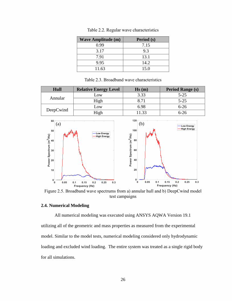
Table 2.2. Regular wave characteristics

Wave Amplitude (m) Period (s)

0.99 7.15

3.17 9.3

7.91 13.1

9.95 14.2

11.63 15.0

Table 2.3. Broadband wave characteristics

Hull Relative Energy Level Hs (m) Period Range (s)

Annular Low 3.33 5-25

High 8.71 5-25

DeepCwind Low 6.98 6-26

High 11.33 6-26

Figure 2.5. Broadband wave spectrums from a) annular hull and b) DeepCwind model

test campaigns

2.4. Numerical Modeling

All numerical modeling was executed using ANSYS AQWA Version 19.1

utilizing all of the geometric and mass properties as measured from the experimental

model. Similar to the model tests, numerical modeling considered only hydrodynamic

loading and excluded wind loading. The entire system was treated as a single rigid body

for all simulations.

(a) (b)

27

Figure 2.6. ANSYS AQWA mesh

A convergence study was performed comparing three possible meshes: one with a

maximum element size of 8.0 m, one with a maximum element size of 4.0 m and the final

case with a maximum element size of 1.5 m. Comparing surge, heave and pitch RAO

results for these three cases yielded similar response predictions with less than a 1%

difference in the maximum RAO values in the wave period range of interest of 5 to 20 s.

Based on these results, the mesh with a maximum element size of 4.0 m was chosen

which featured 2025 nodes and 1980 total elements (see Figure 2.6). A frequency domain

analysis was conducted using this mesh with 90 evenly-spaced wave frequencies ranging

from 0.05 Hz to 0.2 Hz. Mooring line interactions from the experimental setup were

captured using an additional stiffness term in the surge direction of 94.2 kN/m.

In ANSYS AQWA, an external lid was used to account for the motions of the

water within the moonpool geometry. Two parameters are available for customization of

external lid properties, the gap and the damping factor. For this study the gap value was

set to the width of the moonpool per the AQWA User’s Manual (ANSYS Inc., 2013b).

28

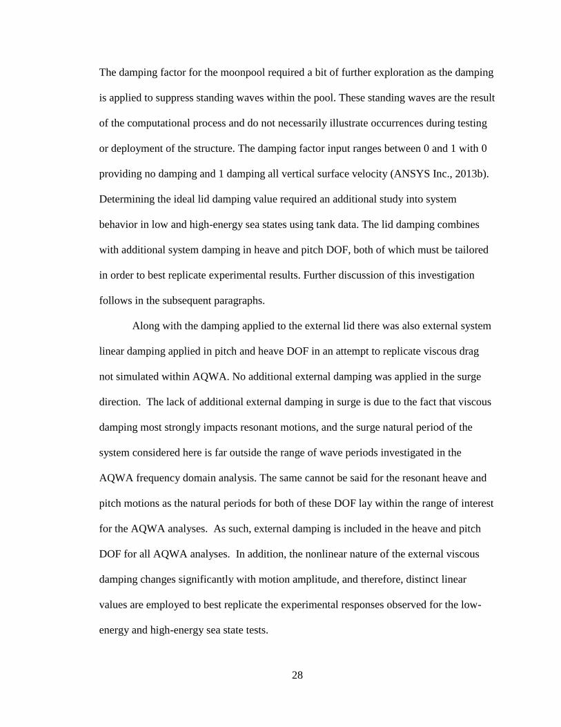
The damping factor for the moonpool required a bit of further exploration as the damping

is applied to suppress standing waves within the pool. These standing waves are the result

of the computational process and do not necessarily illustrate occurrences during testing

or deployment of the structure. The damping factor input ranges between 0 and 1 with 0

providing no damping and 1 damping all vertical surface velocity (ANSYS Inc., 2013b).

Determining the ideal lid damping value required an additional study into system

behavior in low and high-energy sea states using tank data. The lid damping combines

with additional system damping in heave and pitch DOF, both of which must be tailored

in order to best replicate experimental results. Further discussion of this investigation

follows in the subsequent paragraphs.

Along with the damping applied to the external lid there was also external system

linear damping applied in pitch and heave DOF in an attempt to replicate viscous drag

not simulated within AQWA. No additional external damping was applied in the surge

direction. The lack of additional external damping in surge is due to the fact that viscous

damping most strongly impacts resonant motions, and the surge natural period of the

system considered here is far outside the range of wave periods investigated in the

AQWA frequency domain analysis. The same cannot be said for the resonant heave and

pitch motions as the natural periods for both of these DOF lay within the range of interest

for the AQWA analyses. As such, external damping is included in the heave and pitch

DOF for all AQWA analyses. In addition, the nonlinear nature of the external viscous

damping changes significantly with motion amplitude, and therefore, distinct linear

values are employed to best replicate the experimental responses observed for the low-

energy and high-energy sea state tests.

29

After a manual calibration phase employing the free-decay test results, the

additional pitch linear damping values applied in AQWA for this particular system for

low and high-energy wave states were roughly 4% and 13% of critical pitch damping,

respectively. Initial simulation results obtained for the heave RAO magnitudes

demonstrated sensitivities to the variation of external heave linear damping as well as the

damping factor applied to the lid. Based on this finding, these two values were varied

manually to obtain a good fit with the overall surge, heave and pitch RAO experimental

results as the lid damping influenced not only the heave response, but surge and pitch

DOF as well. The results of this study suggest that a heave linear damping of 3% of

critical and a lid damping factor of 0.0001 (i.e. negligible) fit best for the low wave

energy case and a heave linear damping value of 10% of critical combined with a 0.05 lid

damping factor match best with experimental results for the high-energy wave case. The

lid damping factor necessary to generate similar responses to the model test results in

low-energy wave cases suggests that the lid may not even be necessary. By contrast, the

lid damping factor required for high-energy cases indicates that it is highly important in

these situations. The values provided are specific to the hull configuration and

environments presented herein and do not necessarily correspond to the ideal values for

other geometries.

2.5. Results

With the generation of experimental and numerical data complete, the system

responses for both cases can be compared. In addition to this comparison, the comparison

of the annular system with the results from DeepCwind systems is also detailed in the

following sections.

30

2.5.1. Position RAO Magnitudes

When looking at the behavior of a floating wind turbine, the wave-induced

motion of the hull is highly important. For the long-crested waves considered in this

work, the hull DOF of particular concern are surge, heave and pitch. The responses in

these particular DOF play a large role in characterizing a FOWT’s ability to survive the

deep ocean environment as well as minimize wind turbine motions to facilitate smooth

power production. Platforms that minimize wave-induced motions also diminish fatigue

and ultimate loads in the tower, turbine, hull, mooring system and umbilical. To assess

the motion performance of the annular hull FOWT subjected to wave loading, the surge,

heave and pitch RAO magnitudes from both simulation and experiment are presented and

discussed in the subsequent sections.

2.5.1.1. Low-Energy Position RAO Magnitudes

Results from regular wave testing for low-energy waves are shown in Figure 2.8

through Figure 2.10. Shown in Figure 2.8 and Figure 2.9, the irregular wave-derived

RAO magnitude trends follow the regular wave trends for surge and heave fairly well. By

contrast, significant differences between the regular wave and low-energy RAO

magnitudes are found for the 13.1 s and 14.2 s cases for platform pitch. Regular wave

testing at 13.1 s and 14.2 s period caused significant green water, yielding appreciable

nonlinearity in the platform response and likely causing the discrepancy between the

regular and irregular results (e.g. see Figure 2.7). The low-energy white noise wave did

not possess significant green water events, and as such, the experimental data displays a

typical resonant response much like the linear AQWA simulations.

31

Figure 2.7. Overtopping during regular wave 4

The AQWA simulation for the low-energy position RAO magnitudes capture the

overall trends of the experimental results with reasonable accuracy. One notable

difference between these two data sets is in the wave period yielding the peak pitch

response. As seen in Figure 2.10, the largest pitch RAO magnitude occurs at a period of

12.8 s experimentally and 13.2 s in the AQWA model. This discrepancy may be due to

several factors including uncertainty in the measured system pitch inertia, small

differences between the actual and AQWA-calculated added-inertias, and platform pitch

stiffness contributions provided by the mooring system which were not included in the

simulations. Regarding the peak pitch RAO magnitude of Figure 2.10, the difference

between the experimental and AWQA results is only 1.5%.

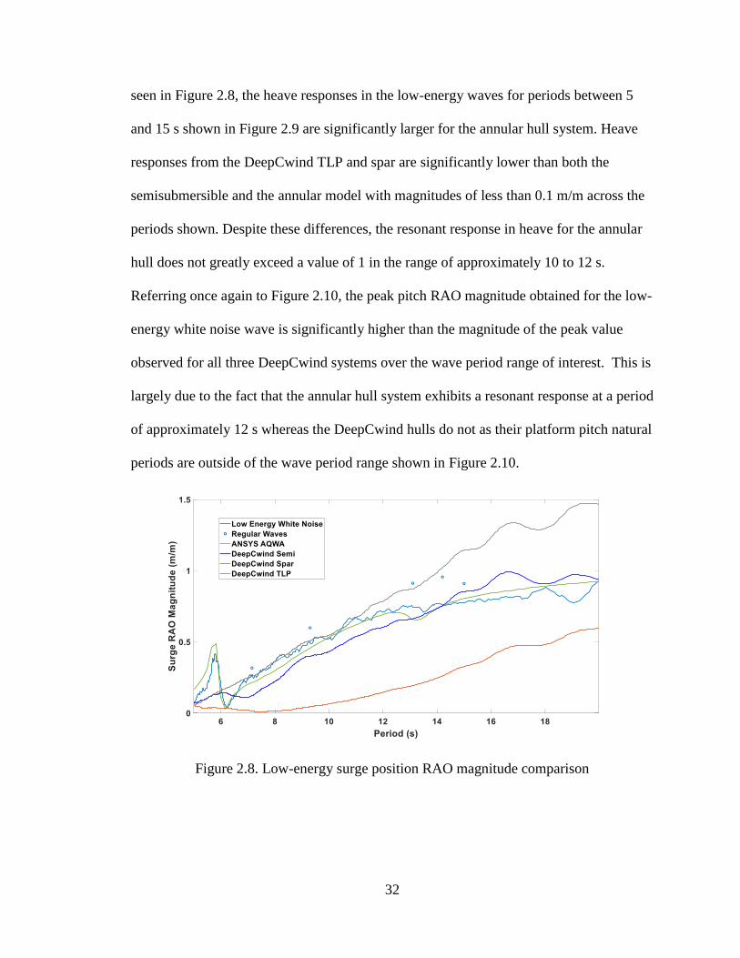
The surge response for the DeepCwind TLP exhibits similar trends to the annular

hull up to a period of approximately 12 s before it departs and maintains a larger

magnitude through the remaining periods of interest. By contrast, the DeepCwind spar

has a significantly lower surge response across all periods of interest. While results for

the annular hull show very similar results to the DeepCwind semisubmersible in surge as

32

seen in Figure 2.8, the heave responses in the low-energy waves for periods between 5

and 15 s shown in Figure 2.9 are significantly larger for the annular hull system. Heave

responses from the DeepCwind TLP and spar are significantly lower than both the

semisubmersible and the annular model with magnitudes of less than 0.1 m/m across the

periods shown. Despite these differences, the resonant response in heave for the annular

hull does not greatly exceed a value of 1 in the range of approximately 10 to 12 s.

Referring once again to Figure 2.10, the peak pitch RAO magnitude obtained for the low-

energy white noise wave is significantly higher than the magnitude of the peak value

observed for all three DeepCwind systems over the wave period range of interest. This is

largely due to the fact that the annular hull system exhibits a resonant response at a period

of approximately 12 s whereas the DeepCwind hulls do not as their platform pitch natural

periods are outside of the wave period range shown in Figure 2.10.

Figure 2.8. Low-energy surge position RAO magnitude comparison

33

Figure 2.9. Low-energy heave position RAO magnitude comparison

Figure 2.10. Low-energy pitch position RAO magnitude comparison

2.5.1.2. High-Energy Position RAO Magnitudes

The high-energy white noise wave-derived position RAO results are shown in

Figure 2.11 through Figure 2.13. As seen in Figure 2.11 and Figure 2.12, the surge and

heave RAO magnitudes derived from the high-energy irregular waves are fairly similar to

34

those for the regular waves, albeit, the comparison is not as good as for the low-energy

heave irregular wave results of Figure 2.9. For the platform pitch RAO of Figure 2.13,

the high-energy white noise compares well with 3 of the 5 regular wave results, with the

two major differences occurring between the two at periods of 13.1 s and 14.2 s. The

cause for the discrepancy is the same as that noted for the results of Figure 2.10.

Comparing the low-energy (Figure 2.8 through Figure 2.10) and high-energy

(Figure 2.11 through Figure 2.13) white noise wave-obtained RAO magnitudes, several

differences can be observed. With increased wave energy, and hence motion amplitude,

it is seen that surge RAO response at a period of approximately 6 seconds is diminished,

likely as a result of resonance of the horizontal sloshing motion within the moonpool.

Additionally, the heave and pitch RAO magnitude peak responses near system resonance

are also diminished (see Table 2.1) at periods of roughly 10 and 13 s, respectively. This is

expected as viscous damping is proportional to the square of the platform velocity. The

increase in hydrodynamic damping for the high-energy sea state most strongly influences

resonant responses of the system, hence the observed differences between the two white

noise wave test RAO magnitudes.

As seen in Figure 2.11, the AQWA simulations match well with the experimental

results in surge. Using an appropriate set of lid and added system damping coefficients in

heave, the AQWA results for the heave RAO magnitudes in this high-energy irregular sea

state compare well with experimental data throughout the entire period range of interest.

The AQWA pitch results demonstrate a slightly higher pitch magnitude with a 3.3%

difference between the peak pitch RAO and the experimental results. While a

discrepancy exists between the AQWA predictions and experimental peak pitch RAO

35

response period for the low-energy white noise wave RAO magnitudes, the difference

between the periods for the high-energy case of Figure 2.13 is much smaller.

Comparing the annular hull and DeepCwind semisubmersible, the two systems

once again exhibit similar surge RAO trends as shown in Figure 2.11. The surge

performance of the spar and TLP as relative to the annular hull system is also very similar

to that found in the low-energy case. Observing the high-energy wave heave RAO

magnitudes (Figure 2.12), it can be seen that the annular hull system possesses

significantly greater heave motion for wave periods in the 10 to 15 s range, with the

DeepCwind semisubmersible exhibiting a greater response for periods of approximately

17 s or larger, this being a period typically outside the peak period of most design sea-

states. The spar and TLP both have lower surge RAO magnitudes than both the

semisubmersible and the annular hull from the period of about 6 s through to the 20 s

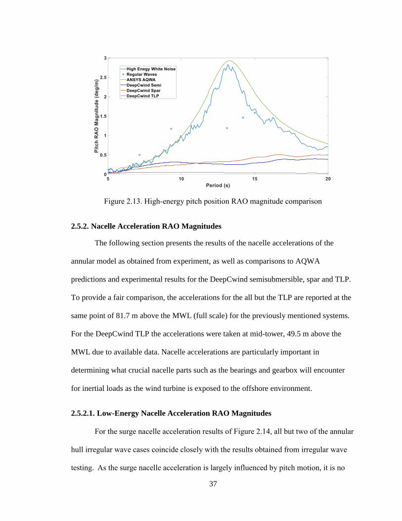
period. Similar to the low-energy wave case, the high-energy case for platform pitch

shows a significant difference between the DeepCwind semisubmersible and the annular

hull system RAO magnitudes with the maximum value of the annular system

approximately seven times that of the DeepCwind system. The DeepCwind spar exhibits

similar pitch performance to the semisubmersible. The platform pitch RAO magnitude of

the TLP is very small, as one would expect, and is less than 0.1 deg/m throughout the

range of periods shown.

36

Figure 2.11. High-energy surge position RAO magnitude comparison

Figure 2.12. High-energy heave position RAO magnitude comparison

37

Figure 2.13. High-energy pitch position RAO magnitude comparison

2.5.2. Nacelle Acceleration RAO Magnitudes

The following section presents the results of the nacelle accelerations of the

annular model as obtained from experiment, as well as comparisons to AQWA

predictions and experimental results for the DeepCwind semisubmersible, spar and TLP.

To provide a fair comparison, the accelerations for the all but the TLP are reported at the

same point of 81.7 m above the MWL (full scale) for the previously mentioned systems.

For the DeepCwind TLP the accelerations were taken at mid-tower, 49.5 m above the

MWL due to available data. Nacelle accelerations are particularly important in

determining what crucial nacelle parts such as the bearings and gearbox will encounter

for inertial loads as the wind turbine is exposed to the offshore environment.

2.5.2.1. Low-Energy Nacelle Acceleration RAO Magnitudes

For the surge nacelle acceleration results of Figure 2.14, all but two of the annular

hull irregular wave cases coincide closely with the results obtained from irregular wave

testing. As the surge nacelle acceleration is largely influenced by pitch motion, it is no

38

surprise that a similar trend is found for the pitch position RAO magnitudes provided in

Figure 2.10 and Figure 2.13. For the heave acceleration RAO magnitudes of Figure 2.15,

the comparison between the white noise and regular wave results is fair.

Comparing the AQWA simulation and experimental results in Figure 2.14, it is

apparent that AQWA performs well giving similar surge acceleration RAO trends as well

as peak response magnitude and period relative to the test data. Moving to Figure 2.15,

the low-energy sea state heave nacelle acceleration RAO results from the model tests and

AQWA show significant similarities, but the two peak values apparent in the white noise

test data appear at lower periods than those from AQWA.

Results for DeepCwind low-energy nacelle acceleration RAO magnitudes shown

in Figure 2.14 and Figure 2.15 are once again significantly lower than those of the

annular model. This is most prominent for the nacelle surge acceleration as the

experimental results for the annular hull possess an RAO magnitude that is in some cases

nearly 90 times greater than the DeepCwind semisubmersible for the wave periods of

interest in Figure 2.14. Comparing all the DeepCwind models to the low-energy white

noise results for the annular hull, all three models have lower surge acceleration RAO

magnitudes for periods ranging from roughly 7 to 15 s. Additionally, the heave

acceleration RAO magnitude of the spar is consistently significantly below the annular

hull with the exception of the roughly 5 and 9 s periods while the TLP heave acceleration

RAO magnitudes are hardly visible due to their extremely small relative magnitude.

39

Figure 2.14. Low-energy nacelle surge acceleration RAO magnitude comparison

Figure 2.15. Low-energy nacelle heave acceleration RAO magnitude comparison

2.5.2.2. High-Energy Nacelle Acceleration RAO Magnitudes

Referring to Figure 2.16 and Figure 2.17, it is observed that the acceleration RAO

magnitudes obtained from the white noise and regular wave tests do not compare as well

as those shown in Figure 2.14 and Figure 2.15. The largest discrepancies occur at low

wave periods. For the low wave periods, the regular wave amplitudes and motions were

40

quite small leading to small hydrodynamic damping in the system. For the large white

noise irregular wave test, the motions were larger leading to larger hydrodynamic

damping, and hence, motion that is likely more strongly damped at these low wave

periods. This difference, coupled with the fact that the acceleration RAO is inversely

proportional to the wave period squared, yields the greater acceleration RAO magnitude

differences observed in Figure 2.16 and Figure 2.17 for small wave periods.

Comparing the AQWA simulations and experimental results of Figure 2.16, it is

seen that the peak RAO magnitude for surge acceleration obtained from the high-energy

irregular wave data and AQWA analysis are similar over the period range of interest

although the magnitude of the AQWA results is noticeably larger from just before the

peak period up through the remaining periods. For the heave nacelle acceleration given in

Figure 2.17, the RAO magnitudes are over-predicted by AQWA in the range of roughly

11 to 14 s. The AQWA results for heave nacelle acceleration do more closely align with

the results obtained for from regular wave testing in this range, however.

With regard to nacelle acceleration of the annular hull system investigated here, it

is clear from the RAO magnitudes provided in Figure 2.16 and Figure 2.17 that the

DeepCwind semisubmersible system has a significantly lower response over a majority

of the period range of interest, particularly for wave periods of 10 s or longer. As was the

case for the low-energy sea state comparison, this is most pronounced for the nacelle

surge acceleration which exhibits peak RAO magnitudes that are several times larger than

the peak heave RAO magnitudes. As shown in Figure 2.16, the annular hull has a lower

surge acceleration RAO magnitude than the DeepCwind spar from 5 to roughly 9 s. The

DeepCwind TLP has a lower response than the annular hull in Figure 2.16 between 7 and

41

18 s. The TLP and spar have a relatively consistent RAO magnitude in heave acceleration

RAO magnitudes across all studied periods, the magnitude of which is lower than the

annular model throughout much of the period range of interest.

Figure 2.16. High-energy nacelle surge acceleration RAO magnitude comparison

Figure 2.17. High-energy nacelle heave acceleration RAO magnitude comparison

2.5.3. Impacts of Heave Plate Addition

The generic design considered here did not consider any heave plates. A

simulation study was conducted with heave plates on the outer perimeter of the hull with

42

a width of 3.44 m for both the high and low energy wave cases. The only changes to the

system were the geometry to account for the heave plates and the calculated viscous

damping. Calculation of viscous damping of the system was kept consistent between the

baseline models and the models with heave plates with pitch and heave damping

corresponding to the percentages of critical as specified previously (4% in pitch and 3%

in heave for the low energy wave case and 13% in pitch and 10% in heave for the high

energy wave case). Maintaining the percentage of critical damping yielded greater actual

damping for the model with heave plates added as the critical damping increases in the

pitch and heave DOF due to the increase in added mass provided by the heave plate. Lid

damping factors of 0.0001 for the low energy wave case and 0.05 for the high energy

case were utilized to maintain consistency with the values utilized in the baseline case.

The simulation mesh included 2868 total elements as compared to 1980 total elements in

the baseline case.

Comparing the baseline case against the case with heave plates suggests that the

heave plates do not significantly impact the RAO magnitudes of interest (Figure 2.18,

Figure 2.19). Peak RAO magnitudes in heave for high and low energy wave cases are

somewhat higher in magnitude with the addition of heave plates, likely due to the

additional wave loading resulting from the plates and their positioning relative to the

water surface. In addition, the low energy wave peak resonance in heave occurs at a

larger period with the addition of the heave plates with little observable difference in the

high-energy case. Peak responses in pitch for both the high and low energy wave cases

are similar with and without heave plates with smaller peak responses at slightly larger

43

periods for the heave plate model. The increase in resonance periods is expected as the

heave plates increase system added mass.

Figure 2.18. ANSYS AQWA heave plate study: Heave RAO magnitude

Figure 2.19. ANSYS AQWA heave plate study: Pitch RAO magnitude

2.6. Discussion

Results from experimental and numerical testing of an annular hull were

presented in this chapter along with results from the 2011 testing of the DeepCwind

44

semisubmersible, spar and TLP. The annular system was sized for a 6-MW equivalent

turbine while the semisubmersible, spar and TLP from the DeepCwind study were sized

for a 5-MW turbine. All results were normalized to account for the discrepancy in turbine

sizing. Performance in the categories of position RAO magnitudes as well as nacelle

acceleration RAO magnitudes were presented for low and high-energy sea states. It

should be noted that the conclusions provided are for the designs as detailed earlier in this

work, and may not be applicable to similar designs. It is important to stress that the

annular hull model tested here is not optimized and it is quite probable that alteration of

system parameters would improve performance. That noted, the DeepCwind FOWT

systems are also generic systems and other, more commercially mature versions of these

designs may exhibit even better global motion performance than the semisubmersible,

spar and TLP comparison data provided here.

2.6.1. Comparison of Response in Low-Energy and High-Energy Sea States

RAO magnitudes derived from low-energy and high-energy white noise wave

testing show several differences worthy of noting. Most of these differences, such as

reduced peak RAO magnitudes in heave or pitch motion near resonance, are due to the

increased platform viscous drag observed in the high-energy sea state testing. These

same trends are also observed for the nacelle heave and surge acceleration RAO

magnitudes. The surge position RAO magnitude does not vary significantly between the

two white noise tests, however, as the surge natural period is far outside the wave periods

investigated.

45

2.6.2. Discrepancy between RAO Magnitudes Derived from Irregular Waves and

Regular Waves

For the pitch position and surge acceleration RAO magnitudes, some significant

deviation occurs between the regular wave results and the white noise wave results at

13.1 s and 14.2 s wave periods. As these particular periods are close to the natural period

of the system in pitch, significant pitch motion occurs which allowed for modest to large

amounts of green water and overtopping for these two regular wave test cases (e.g. see

Figure 2.7). This significant nonlinear behavior did not manifest itself in the irregular

wave cases leading to the significant difference in the two sets of results.

2.6.3. ANSYS AQWA Modeling Capability

This study shows that the use of ANSYS AQWA can provide fairly accurate

results for the hydrodynamic response of an annular floating hull. That noted, the

accuracy of the results obtained from ANSYS AQWA are dependent on proper tuning of

the lid damping factors and external added damping. The values utilized here, while

perhaps applicable to a range of potential annular hull designs, are specific to the

geometry and wave environments considered in this work.

2.6.4. Performance Comparison for Annular Hull and DeepCwind Platforms

In general, the RAO magnitudes associated with the annular hull are larger than

those of the DeepCwind data set. There are a few cases where the annular hull does

perform similarly to the other studied systems, namely in surge RAO magnitudes in the

range of roughly 15 s to 20 s. The pitch RAO magnitudes in the high and low portions of

the period range considered are also fairly similar across all 4 models.

46

2.6.5. Influence of Heave Plates on Performance

The addition of heave plates resulted in minimal impacts to the system

performance. Although the peak response period in heave for the low energy case was

extended, the magnitude of system response increased. On a positive note, the period of

peak pitch response was extended for both the low and high energy wave cases.

Additionally, the magnitude of the pitch response decreased in both cases. The heave

plates modeled herein suggest that further optimization would be necessary for improved

performance.

47

CHAPTER 3

COMPARATIVE STUDY OF ANNULAR FOWT HULL GEOMETRIES

3.1. Development of Hull Alternatives

With the performance of a baseline hull quantified, the next step was to explore

the impacts of adjusting the geometry. The first portion of geometric adjustments,

explored in the following chapter, involves three alternative annular hulls as well as

comparison to a basic barge.

3.1.1. Shape Variations

A comparison study of four generic hull geometries was completed to determine

the linear hydrostatic stability and rigid-body natural frequencies in the platforms’ heave

and pitch DOF of each system. Added mass values in surge, heave and pitch are also

discussed. Three of the geometries were variations of the annular hull concept: a square

prism with a square moonpool, a cylinder with a circular moonpool and a triangular

prism with a triangular moonpool. A barge was also studied for a baseline perspective on

the effectiveness of adding a moonpool. These options were selected for their relative

simplicity, but also for their stark differences in geometry which strongly influences the

hydrodynamic loading and moonpool dynamics.

3.1.2. Stability Requirements and Standardized Parameters

All geometries were sized to support a 6-MW turbine with the baseline case taken

from Section 2.1. When designing FOWTs, one of the main design constraints is the

system’s response in rotation about the horizontal axis due to wind and wave loads. As a

result, significant focus falls on the pitch RAO. One major factor in determining the pitch

RAO is the pitch waterplane stiffness (𝐾𝑝𝑖𝑡𝑐ℎ ℎ𝑦𝑑𝑟𝑜); this characteristic is not frequency

48

dependent and can be calculated knowing the dimensions of the hull and ( 3.1) (Jonkman,

2007).

𝐾𝑝𝑖𝑡𝑐ℎ ℎ𝑦𝑑𝑟𝑜 = 𝜌𝑔 ∬ 𝑥2𝑑𝐴 + 𝜌𝑔𝑉𝑧𝑏 − 𝑚𝑡𝑜𝑡𝑔𝑧𝑔 + 𝐾𝑝𝑖𝑡𝑐ℎ 𝑚𝑜𝑜𝑟𝑖𝑛𝑔 ( 3.1 )

Where: 𝜌 is the density of sea water

𝑔 is the gravitational constant

∬ 𝑥2𝑑𝐴 is the area moment of inertia of the waterplane

𝑉 is the submerged volume

𝑧𝑏 is the vertical distance to the center of buoyancy

𝑚𝑡𝑜𝑡 is the total mass

𝑧𝑔 is the vertical distance to the center of gravity

𝐾𝑝𝑖𝑡𝑐ℎ 𝑚𝑜𝑜𝑟𝑖𝑛𝑔 is the pitch mooring stiffness (which is negligible for this analysis)

The pitch waterplane stiffness was calculated for the baseline case and was held constant

along with hull height, draft, cross-section width and hull density as well as the other

values specified in Table 3.1 and illustrated in Figure 3.1 for all of the designs considered

in this section.

Table 3.1. Shape variation standardized parameters

Parameter Magnitude

Hub Height 100 m

Rotor Diameter 150 m

Turbine Mass 440 t

Tower Mass 520 t

Draft 11.6 m

Pitch Waterplane Stiffness 4,631,000 kN·m/rad

mhull/mballast 7.2

Hull Density 768.0 kg/m3

49

Figure 3.1. Standardized parameter visual

3.2. Shape Comparison Resulting Geometries

Resulting dimensions for the triangular, circular, and barge hulls were determined

using the Solver add-on in Excel. The Solver objective value was set as the pitch

waterplane stiffness of 4,630,000 kN·m/rad. The dimensional variable for the barge and

triangular hulls were the corresponding outer side lengths. For the circular hull the

dimensional variable was the outer radius. The variable dimensions were adjusted while

maintaining the standardized values from Table 3.1 in order to obtain a design with the

desired pitch stiffness. The resulting characteristics are shown in Table 3.2 and Figure

3.2. Figure 3.2 shows the footprints of the hulls with the original square (with moonpool)

shown in blue, the triangle in orange, the circle in green, and the outer perimeter of the

barge (no moonpool) shown in black. As shown in Table 3.2, the circular hull provides

the lowest total mass, the shortest outer perimeter, and the maximum moonpool area. By

contrast, the triangular hull represents the highest total mass (of the hulls with

moonpool), longest outer perimeter, and smallest moonpool area.

50

Table 3.2. Selected resulting parameters

Geometry

Total

Mass

(t)

Floater

Mass

(t)

Hull

Mass

(t)

Ballast

Mass

(t)

Outer

Perimeter

(m)

Moonpool

Area (m2)

Square 21,341 20,386 17,888 2,498 210 956

Square (no

moonpool) 30,638 29,683 26,046 3,637 205 --

Triangle 21,911 20,956 18,388 2,568 228 641

Circle 20,154 19,199 16,847 2,353 191 1,209

Figure 3.2. Resulting footprints

Additional calculations were completed to determine the inertial inputs for

AQWA analysis. Among these are the total system mass, the mass moment of inertia in

pitch and yaw about the FOWT’s center of gravity and the location of the center of

gravity. Inertia values were calculated through the application of the parallel-axis

theorem and the assumed mass properties of the hull cross section in Figure 3.1. In

general, it was assumed that the hull had uniform density with the exception that the mass

of the turbine and tower was also applied in the hull body at a location which mirrored

51

the surge and sway coordinates of the physical location of the turbine and tower on the

horizontal plane. The resulting pitch and yaw mass moments of inertia are given by Table

3.3. For all hulls the center of gravity in the horizontal plane was assumed to be at the

intersection of the surge and sway axes. The center of gravity in the vertical (heave)

direction was dependent on the mass of the hull and varied from hull to hull as a result;

these values are given in Table 3.3 with z = 0 falling at the mean water line (MWL) for

each hull.

Table 3.3. Shape variation inertias and center of gravity locations

Geometry Pitch Inertia

(kgm2)

Yaw Inertia

(kgm2)

Vertical Center of

Gravity location (m)

Square 1.149 × 1010 1.859 × 107 -1.053

Square (no moon pool) 1.184 × 1010 1.380 × 1010 -2.024

Triangle 8.330 × 109 8.848 × 109 -1.136

Circle 1.181 × 1010 1.268 × 1010 -0.865

3.3. ANSYS AQWA Parameters

The following section will discuss the settings applied during modeling in

AQWA. Justifications for each setting are also provided.

3.3.1. Mesh Sizing

Per the convergence study completed in the numerical modeling section (Section

2.4), a sufficiently refined mesh was applied to each of the models studied herein. All

four of the models were meshed with a defeaturing tolerance of 1 m and a maximum

element size of 4 m. Table 3.4 specifies the total number of nodes and elements for all

four hull forms.

52

Table 3.4. Mesh characteristics

Geometry Number of Nodes Number of Elements

Square 2025 1980

Square (no moon pool) 969 924

Triangle 1265 1216

Circle 1847 1806

3.3.2. Modeling Parameters

The global response of the four systems of interest were simulated in ANSYS

AQWA with the moonpools modeled using the external lid feature. Each geometry was

subjected to a range of wave periods from 5 s to 20 s in increments of 0.23 s. The waves

were applied along the surge direction at 0 degrees (see Figure 3.3). For the triangular

hull the waves approached from the broad side. In addition to the runs completed in

AQWA, the same parameters were applied to the square annular hull model and run in

the commercial modeling software WAMIT as verification for the ANSYS AQWA

results for the heave and surge RAO results.

Figure 3.3. Square annular hull with wave directions

53

3.3.3. Assumptions and Simplifications

Each hull supported a 6-MW turbine with a mass of 438 metric tons. The turbine

tower mass was also standardized at 517 metric tons. In the sizing process the hull height,

draft, cross-section width and hull density were kept consistent across all four designs.

The effects of mooring lines were not included in this study as they have a negligible

impact on system motions in the wave frequency region.

The additional external damping due to viscous effects was tuned for the high

energy set of wave cases as prescribed by section 2.4. As such, the external damping

inputs were approximated similarly across all models. The damping for each model was

determined using a damping ratio of 10% of the critical damping in heave and 13% of the

critical damping in pitch with critical damping calculated as specified in ( 3.2 ) (Inman,

2001).

𝜁 = 𝑐

𝑐𝑐𝑟=

𝑐

2√𝐾𝑖𝑚𝑡𝑜𝑡

( 3.2 )

Where: 𝑐 is applied damping

𝑐𝑐𝑟 is critical damping

𝐾𝑖 is the stiffness in pitch or heave

𝑚𝑡𝑜𝑡 is the mass (or inertia in the case of pitch)

ζ is the damping ratio

The heave critical damping is approximately equal to the value utilized for the high

energy sea state and the pitch critical damping value is approximately equal to that

utilized for the low energy sea state in section 2.4. Additionally, all three annular hulls

utilized a value of 0.05 for the lid damping factor matching the value specified for high

energy sea states in section 2.4 (see Chapter 2 for impacts of varying this value). Per the

ANSYS User’s Manual the width of the lid was specified as the width across the

54

moonpool (ANSYS Inc., 2013b). In the case of the triangular and circular hulls the

widths were taken as the mean width across the corresponding moonpool.

As noted previously, the study completed only considered unidirectional waves.

The wave cases considered here run along the x axis. The wave in the zero-degree

direction was used to generate all RAO magnitude plots which represent a wave running

from the positive x-direction to the negative x-direction. In the case of the offshore

environment it would be important to consider waves from multiple directions,

particularly in the case of the square and triangular systems as the geometry is not

symmetric and would likely change the system response more than the symmetrical

circular system.

3.4. Results

With the system geometries determined, additional system characteristics were

calculated and compared with AQWA results. The natural periods, added masses, and

RAO magnitudes for each geometry are specified below.

3.4.1. Natural Periods

Following the determination of the dimensions, the pitch and heave natural

periods were calculated manually as part of the comparison and verification process. The

pitch natural periods (𝑇𝑛𝑝𝑖𝑡𝑐ℎ) were calculated according to ( 3.3 ) (Halkyard, 2013). The

heave natural periods (𝑇𝑛ℎ𝑒𝑎𝑣𝑒) were calculated according to ( 3.4 ) (Halkyard, 2013). The

results of these calculations are shown in Table 3.5.

55

𝑇𝑛𝑝𝑖𝑡𝑐ℎ= 2𝜋√

𝐾𝑝𝑖𝑡𝑐ℎ ℎ𝑦𝑑𝑟𝑜 + 𝐾𝑝𝑖𝑡𝑐ℎ 𝑚𝑜𝑜𝑟𝑖𝑛𝑔

𝐼𝑝𝑖𝑡𝑐ℎ + 𝐼𝑝𝑖𝑡𝑐ℎ 𝑎𝑑𝑑𝑒𝑑 ( 3.3 )

Where: 𝐾𝑝𝑖𝑡𝑐ℎ ℎ𝑦𝑑𝑟𝑜 is the pitch stiffness

𝐾𝑝𝑖𝑡𝑐ℎ 𝑚𝑜𝑜𝑟𝑖𝑛𝑔 is the mooring stiffness in pitch (considered negligible)

𝐼𝑝𝑖𝑡𝑐ℎ is the pitch inertia of the system

𝐼𝑝𝑖𝑡𝑐ℎ 𝑎𝑑𝑑𝑒𝑑 is the pitch inertia of the added mass per AQWA

𝑇𝑛ℎ𝑒𝑎𝑣𝑒

= 2𝜋 √𝐾ℎ𝑒𝑎𝑣𝑒 ℎ𝑦𝑑𝑟𝑜 + 𝐾ℎ𝑒𝑎𝑣𝑒 𝑚𝑜𝑜𝑟𝑖𝑛𝑔

𝑚𝑡𝑜𝑡 + 𝑚ℎ𝑒𝑎𝑣𝑒 𝑎𝑑𝑑𝑒𝑑

( 3.4 )

Where: 𝐾ℎ𝑒𝑎𝑣𝑒 ℎ𝑦𝑑𝑟𝑜 is the pitch stiffness

𝐾ℎ𝑒𝑎𝑣𝑒 𝑚𝑜𝑜𝑟𝑖𝑛𝑔 is the mooring stiffness in heave (considered negligible)

𝑚𝑡𝑜𝑡 is the mass of the system

𝑚ℎ𝑒𝑎𝑣𝑒 𝑎𝑑𝑑𝑒𝑑 is the added mass in heave per AQWA

Table 3.5. Pitch and heave calculated natural periods

Geometry Pitch Natural

Period (s)

Heave Natural

Period (s)

Square 11.6 10.1

Square (no moon pool) 11.9 11.2

Triangle 10.4 10.2

Circle 11.7 9.3

These calculated values serve as approximate values for the location of peak

values on the pitch and heave RAO plots which indicate resonance. Because each of

these periods is calculated considering a fixed approximation of the added mass—which

is actually frequency dependent—the exact period with maximum response can be

somewhat different than the natural period.

3.4.2. ANSYS AQWA Added Mass

Components of added mass reflect the mass of the volume of water that moves

when the structure moves. Added mass is one factor in determining how a system will

respond in a wave environment. The plot of the surge added masses (Figure 3.4) shows

that the circular hull has the highest peak value for surge added mass. However, all three

56

designs with moonpools have approximately the same added mass at the 20 s wave

period (~2.5 × 107 kg). As the surge natural period of these systems when moored tends

to be quite long, the results of Figure 3.4 indicate that the contribution of the surge added

mass of all three systems to the natural period is effectively the same, which given their

similar physical masses, indicates that all three systems will likely exhibit near equal

surge natural periods. Comparing the barge and annular hull systems, the faces of the

moonpools for the models that have them contribute additional added mass, hence the

increase in surge added mass relative to the barge system.

Figure 3.4. Shape variation surge added mass

The plot of the heave added masses (Figure 3.5) shows that of the four geometries

simulated, the barge has a significantly higher value for heave added mass at all

evaluated periods. The triangular hull has the second highest and square hull and circular

hulls are the third and fourth largest, respectively. For this DOF it seems reasonable for

the barge to have the highest value of added mass as it has the largest waterplane area.

57

Figure 3.5. Shape variation heave added mass

A plot of the pitch added inertias for the systems studied (Figure 3.6) shows that

the circular hull has the highest peak magnitude. Again, all three designs with moonpools

have approximately the same added inertias as the wave periods increase. In this case the

barge has the highest added inertia. The added inertias in the pitch DOF are dependent in

part on the waterplane area of the hull (hence the gap from the moonpool hulls to the

barge), but also on the way this area is distributed. As the barge water plane area is not

only solid, but also has a perimeter almost similar in size to the other designs, it is not

surprising that the pitch added mass is in general larger than the annular hull systems for

most wave periods studied.

58

Figure 3.6. Shape variation pitch added inertias

3.4.3. ANSYS AQWA Response Amplitude Operators

The physical response of the structure due to interactions with the waves is a

critical design consideration. As a result, RAO magnitudes for three DOFs (surge, heave,

and pitch) hold a substantial amount of weight in the comparison process. As shown in

Figure 3.7, the barge has the highest peak surge RAO magnitude.

Figure 3.7. Shape variation surge RAOs

59

All four models exhibit a similar trend of increasing RAOs with increasing periods with

two separate downward trends. One of the downtrends is at roughly the 6 s period. For

the square annular design, this downtrend is very close to the sloshing natural frequency

of the moonpool of 6.35 s. In the cases of the triangular and circular hulls, the sloshing

natural frequency is a bit more difficult to calculate as the equation for calculating the

natural frequency uses the width of the moonpool as an input. When referring to the

square geometry, it is reasonable to say that the “width” of the moonpool is the side

length. For the circular hull, the moonpool does not have any faces which would be

categorized as sides in the same way, but approximating the width to be the average

width of the circle results in an approximate natural period for the sloshing mode of 6.36

s which is in general agreement with the observations of the ANSYS AQWA simulation

results. In the case of the triangle, for the wave at zero degrees, the side length of the

moonpool varies from 0 m at the point to 38.47 m at the side of the triangle. Considering

the width to be the average width of the moonpool results in a sloshing natural period of

7.98 s; the AQWA results suggest that a value of 6 s is more realistic. The second

downtrend is near the 12 second period (10 seconds for the triangular hull). This

downtrend is likely due to a canceling effect as the length of the hulls in the surge

direction is similar to the wavelength associated with the period.

Each of the moonpool hulls has a notable drop in the heave RAO (Figure 3.8) at a

similar period. It is likely that this slight dip is influenced by the natural period of the

moonpool piston period. The calculated piston natural period values (per section 1.2.3)

for the moonpools of the square, triangular and circular hulls are 9.88 s, 9.40 s, and 10.20

s, respectively. The calculated heave natural periods of the systems are 10.09 s, 10.19 s,

60

and 9.27 s, respectively, which are very close to the predicted piston periods. By contrast,

the periods in the low point of the dips for the three annular hull heave RAOs occur at

8.27 s, 8.36 s, and 8.46 s, these values not aligning with the anticipated heave periods or

moonpool piston periods. This discrepancy suggests that this dip is caused by coupling

between the resonant vertical motions of the hull and the water in the moonpool. Overall,

the circular hull has the highest peak heave RAO magnitude and it is followed by the

square, triangular, and barge hulls, respectively. The heave RAOs for all four systems at

large periods are almost identical. Although the barge system does not seem to

experience the damping that the annular hulls do, it does outperform the other systems

across the full range of the periods with the exception of the periods in proximity to the

downtrends from the other hulls where the moonpool piston motion damps the hull

motion.

Figure 3.8. Shape variation heave RAOs

The pitch RAO magnitudes shown in Figure 3.9 suggest that the geometry does

not have a significant impact when comparing the square, barge, and circular hulls. The

peak values for each of these geometries are all very similar. On the other hand, the peak

61

value and peak period of the triangular hull response are both slightly lower than the rest

of the group. The pitch DOF is not considered to be significantly influenced by the

moonpool as calculated pitch natural periods align well with peak values from Figure 3.9.

Calculated values for the square, triangular and circular hulls are 11.56 s, 10.36 s, and

11.66 s respectively while the peak values from AQWA are 11.76 s, 10.60 s, and 11.92 s.

Figure 3.9. Shape variation pitch RAOs

3.5. Discussion

The results of this study suggest that there is not a significant difference in the

global performance as determined by RAO magnitudes for the four modeled systems in

surge, heave, or pitch DOF. It does show, however that using the outer dimensions of a

barge system and transitioning it into an appropriately-sized annular hull can significantly

reduce the volume of material needed to support a turbine of equal size. In comparing the

three annular hulls the square and circular hulls performed very similarly across all three

RAOs. The triangular hull had a larger surge response than the square and circular hulls

from roughly 7 s to 10 s. Although the peak response in pitch for the triangular hull is

62

smaller in magnitude than the circular and square hulls this is not enough to make up for

the impracticality in fabricating a hull with a larger footprint. The final comparison

between the circular and square hulls considers the ease of fabrication and storage along

with transportability. From a manufacturing standpoint the square hull is considered to be

better as it can be manufactured in segments using primarily right angles and forms that

feature the same. By comparison, fabrication of the circular model would require arched

forms to produce the circular shape which are not readily available. In addition to this,

the maneuverability of a square is easier when considering moving the hull around dry

docks and other port facilities dues to the general shape of the environment as well as its

side length which offers a smaller minimum dimension. Based on consideration of these

additional areas of interest, the square hull is the superior option and is chosen as the

ideal hull of those tested.

63

CHAPTER 4

SIZING OPTIMIZATION OF SQUARE ANNULAR HULL

4.1. Introduction

The intent of the following optimization was to design an efficient, high-

performance annular FOWT hull through the minimization of the pitch natural frequency

and system mass using a Genetic Algorithm (GA) documented in Goupee and Vel

(Goupee & Vel, 2007). The GA from Goupee and Vel uses a particular real-coded elitist

non-dominated sorting multi-objective GA know as NSGA-II (Non-dominated Sorting

Genetic Algorithm-II) from the work of Deb et al. (Deb et al., 2000). NSGA-II was

created to combat the typical shortfalls of NSGA including its high computational

demand and lack of elitism. Goupee and Vel utilized this GA to optimize the functional

grading of materials to best utilize the inherently inhomogeneous material properties.

4.2. Optimization Problem Statement

The general form of a constrained optimization problem includes design variables

to be modified, bounds on those variables, functions to be optimized, and constraints on

the results. The complete problem statement for this optimization problem is as follows:

Find 𝑃1, 𝑃2, 𝑃3, and 𝑃4

Minimize 𝑓1 =𝑚𝑡𝑜𝑡

𝑚𝑛𝑜𝑚 & 𝑓2 =

√𝐾𝑝𝑖𝑡𝑐ℎ ℎ𝑦𝑑𝑟𝑜

𝐼𝑝𝑖𝑡𝑐ℎ+𝐼𝑝𝑖𝑡𝑐ℎ 𝑎𝑑𝑑𝑒𝑑

𝜔𝑝𝑖𝑡𝑐ℎ 𝑛𝑜𝑚

Subject to

𝑔1 = 7 𝑚 − 𝑡

𝑡𝑛𝑜𝑚 ≤ 0

𝑔2 = ℎ𝑒𝑖𝑔ℎ𝑡 − 𝑑𝑟𝑎𝑓𝑡

𝑑𝑟𝑎𝑓𝑡𝑛𝑜𝑚≤ 0

𝑔3 = −𝐾𝑝𝑖𝑡𝑐ℎ ℎ𝑦𝑑𝑟𝑜

𝐾𝑝𝑖𝑡𝑐ℎ 𝑛𝑜𝑚≤ 0

64

𝑔4 = 𝜃𝑃𝑖𝑡𝑐ℎ − 10°

10°≤ 0

𝑔5 = 2 𝑚 − 𝑓𝑟𝑒𝑒𝑏𝑜𝑎𝑟𝑑

2 𝑚≤ 0

10 𝑚 < 𝑃1 < 60 𝑚

30 𝑚 < 𝑃2 < 74 𝑚

0 𝑚 < 𝑃3 < 15 𝑚

5 𝑚 < 𝑃4 < 30 𝑚

Where: 𝑃1, 𝑃2, 𝑃3 & 𝑃4 are hull geometric parameters (see Figure 4.1)

𝑚𝑡𝑜𝑡 is system mass, kg

𝑚𝑛𝑜𝑚 is mass of baseline system without heave plates, kg

𝐾𝑝𝑖𝑡𝑐ℎ ℎ𝑦𝑑𝑟𝑜 is pitch stiffness, N·m/rad

𝐼𝑝𝑖𝑡𝑐ℎ is pitch inertia, kg·m2

𝐼𝑝𝑖𝑡𝑐ℎ 𝑎𝑑𝑑𝑒𝑑 is pitch inertia from the added mass, kg·m2

𝜔𝑃𝑖𝑡𝑐ℎ 𝑛𝑜𝑚 is nominal pitch natural frequency, rad/s

𝑡 is hull thickness, (P2-P1)/2, m

𝑡𝑛𝑜𝑚 is nominal hull thickness, m

ℎ𝑒𝑖𝑔ℎ𝑡 is hull height, m,

𝐾𝑝𝑖𝑡𝑐ℎ 𝑛𝑜𝑚 is nominal pitch stiffness, N·m/rad

𝜃𝑃𝑖𝑡𝑐ℎ is platform pitch angle under wind turbine thrust at rated wind speed, degrees

𝑓𝑟𝑒𝑒𝑏𝑜𝑎𝑟𝑑 is distance from waterline to top of hull, m

4.2.1. Objective Functions

The objective functions are 𝑓1 and 𝑓2. The mass ratio (𝑓1) is calculated by taking

the mass of the proposed geometry and comparing it to the nominal mass of 2.134 × 107

kg as described in the model specifications in Table 2.1. The benefits of mass reduction

include a smaller footprint and material reduction, both of which are important to

reducing cost and easing the burdens of transportation and installation. The pitch natural

frequency ratio (𝑓2) is calculated by taking the pitch natural frequency of the system (the

square root of the pitch stiffness divided by the pitch inertia) and dividing it by the

nominal pitch natural frequency of 0.544 rad/s (or 0.087 Hz) per the specified value from

Table 2.1. Minimizing the FOWT’s rigid-body pitch natural frequency ratio results in

65

increasing the pitch natural period of the system further. Longer natural pitch periods are

helpful in preventing resonance from the excitation of typical offshore sea state

conditions. The intent is to minimize both of these functions, but their ideal geometries

compete; that is to say that for the pitch natural frequency of 𝑓2 to decrease, the mass

ratio of 𝑓1 is typically increased and vice versa. The competition between these two

objective functions makes this scenario a prime candidate for the multi-objective

optimization provided by NSGA-II.

4.2.2. Design Variables and Corresponding Bounds

For this case, the design variables of the hull which are subjected to optimization

techniques are 𝑃1, 𝑃2, 𝑃3, and 𝑃4, as illustrated in Figure 4.1.

Figure 4.1. Top-down and section view of hull

The thickness of the heave plate (shown in grey in Figure 4.1) is kept consistent across all

variations at a value of 0.457 m per industry recommendation. The heave plate is always

mounted with its lower edge aligned with the base of the hull. Additional constants are

listed in Table 4.1. Hull density is an average value assuming that the ballast is evenly

distributed throughout the hull. The design variables will be used to determine the system

mass, center of gravity, mass moments of inertia, and natural period in pitch using

MATLAB.

66

Table 4.1. Constant values

Constant Value (kg/m3)

Sea Water Density 1,025

Hull Density 768

Plate Density 1,895

The calculation of system mass is based on the volume of the hull multiplied by

the density and adding that to the product of the plate density and volume as well as the

turbine and tower masses. The center of gravity of the system uses the masses of each of

the components coupled with each of their corresponding center of gravity in the

horizontal 𝑥 and vertical 𝑧 directions relative to aft left corner on the mean waterline.

The pitch natural period of the system is highly dependent on the pitch stiffness

which was previously defined in Chapter 3 and is driven by the waterplane area,

submerged volume and vertical position of the center of gravity. The other input for the

pitch natural period is the pitch inertia. The pitch inertia of the hull and heave plate are

derived from component inertias.

In addition to the system itself, there is also the influence of the added mass on

the inertia of the hull. Added mass is an additional resistance to motion of a body in a

fluid which is the result of the acceleration of the body. The added masses are

approximated for the purposes of this analysis according to guidelines from Appendix D

of Det Norske Veritas RP C205 (Det Norske Veritas, 2014) as well as the parallel axis

theorem. Utilized added mass coefficients are given in Table 4.2 with the relevant

equation for added mass (𝑚ℎ𝑒𝑎𝑣𝑒 𝑎𝑑𝑑𝑒𝑑) given in ( 4.1 ). All calculations are detailed in

the MATLAB scripts in Appendix A.

67

Table 4.2. Added mass coefficients

Hull Cross

Section

𝒕

𝒉

Direction of

Motion 𝑪𝑨 𝑨𝑹

∞

Vertical

1.0

𝜋 (𝒕

𝟐)

𝟐

10 1.14

5 1.21

2 1.36

1 1.51

0.5 1.70

0.2 1.98

0.1 2.23

Where: ℎ is hull draft or heave plate thickness

𝑡 is hull thickness or heave plate width

𝑚ℎ𝑒𝑎𝑣𝑒 𝑎𝑑𝑑𝑒𝑑 = 𝜌𝐶𝐴𝐴𝑅 ( 4.1 )

Where: 𝑚ℎ𝑒𝑎𝑣𝑒 𝑎𝑑𝑑𝑒𝑑 is heave added mass of from the hull or heave plates

Restrictions on the geometry come from bounds which are specific to the

variables themselves. Upper and lower bounds on 𝑃1, 𝑃2, 𝑃3, and 𝑃4 are given in the

problem statement in section 4.2. The intent of the bounds is to keep the footprint and

hull height values from becoming unreasonable or unrealistic, mostly from a

manufacturing perspective. Additionally, variables are kept in the positive design space

to allow for physical existence of the hull. The width of the moonpool (𝑃1) can vary from

10 m to 60 m. The lower bound forces the existence of the pool while the high end of the

range coupled with the upper bound of the hull width (𝑃2) of 74 m helps to ensure both a

comparable or more efficient footprint as well as the ability to support the diameter of the

base of the wind turbine tower. The lower bound on the hull width (30 m) is slightly

smaller than the width of the hull for a 2-MW turbine, allowing hulls with smaller widths,

68

but other geometric variations to be explored. The heave plate width (𝑃3) is permitted to

vary from 0 m to 15 m, representing the hull as tested and numerically validated in

Chapter 2 as well as the potential for the addition of heave plates. Upper and lower

bounds on the height of the hull force the hull to be a maximum of a typical hull height

for a 6-MW FOWT hull of 30 m and at a minimum to be able to have a 3 m draft while

allowing 2 m of freeboard. In addition to the justifications provided above, the bounds

serve to expedite the evaluation as their existence reduces the design space to a more

manageable volume for the scope of this task.

4.2.3. Constraints

While the objective functions set the stage for the problem to be solved, the

constraint functions form guidelines on the geometry and basic system performance. The

first constraint function (𝑔1) serves to ensure that the side lengths of the moonpool are

smaller than those of the hull, thereby allowing for the physical existence of the system.

The second constraint function (𝑔2) forces the draft of the system to be less than the

height of the hull, which guarantees that the system can float. The purpose of the third

term (𝑔3) is to drive the pitch stiffness of the design to be greater than zero; a condition

which would present no resistance to overturning. Constraint function 𝑔4 serves to help

maintain the static pitch displacement to be no more than 10 degrees under a baseline

wind loading case. This constraint is based on maximizing wind turbine functionality, as

tilted rotors capture less energy and turbine manufacturers do not design their turbines to

function for scenarios where the turbine is tilted far from perfectly vertical. The final

constraint (𝑔5) pushes designs to feature a freeboard which will experience limited

greenwater in day to day operations. Each of the five constraints will yield unique values

69

for each combination of design variables depending on the degree of violation for any

particular value. The resulting values of each of the five constraint functions are summed

to form one total constraint value.

4.3. Use of NSGA-II Optimization Technique

Using the NSGA-II optimization technique, the first step in finding an optimal set

of solutions is to generate a random population of 𝑁 individuals; for this optimization 𝑁

is 100. These individuals represent a chromosome made up of the four design variables

(genes). Each individual is evaluated against the two objective functions to determine

their fitness. The individuals are also evaluated to obtain a measurement of constraint

violation. For this formulation, the constraint violation is applied as a constraint value

(𝑐𝑣) which represents the sum of the values of each constraint function as shown in

section 4.2.

The goal of this optimization is to generate a set of possible geometries for the

objective functions known as Pareto-optimal solutions or a Pareto front. These solutions

represent a population which is non-dominated throughout the feasible design space

(Pareto, 1971). For some individual A to constrain-dominate some individual B, any one

of a set of the following three conditions must be true:

1. Both A and B are feasible, with

a. A being no worse than B in all objectives

b. A is better than B in at least one objective

2. A is feasible and B is not

3. A and B are both infeasible, but B has a larger constraint violation

If none of the three conditions are true, A and B are non-dominated (Goupee & Vel,

2007).

70

Even if a solution is considered to be dominated within the current generation, it

can still be carried through to the next generation. After each member of the population

is evaluated, they are given a rank of non-constrain-domination. Non-dominated

individuals are given a rank of 1; individuals which are only dominated by those

individuals with a rank of 1 are given a rank of 2, and so on. This rank will be applied

later in the process.

An additional factor in the selection of individuals is the crowding distance.

Crowding distance is a measure of proximity of an individual to neighbors of equal rank.

Evaluating the crowding distance encourages a more diverse population which helps to

ensure that a variety of possible solutions are evaluated. The metric used here is taken

from Deb et al. (Deb et al., 2000).

Once the population has been established, the next goal is to create an offspring

population. For a multi-objective GA, this means the creation of a mating pool. The

mating pool represents the population from which the parents of the next generation will

be selected. To determine which individuals enter the mating pool, two individuals from

the population of size N are selected at random to compete in a tournament. The winner

between some individual A and some individual B is the individual with the better rank

or the individual with the larger crowding distance in the event that they have the same

rank. A copy of the winner is added to the mating pool. This process is complete when

each individual has competed twice and the mating pool consists of N parents. As a

result of the tournament selection process the mating pool now contains more copies of

stronger individuals and fewer copies of weaker individuals.

71

The creation of the next generation is completed next by randomly choosing two

parents from the mating pool and applying simulated binary crossover (SBX) and the

real-parameter mutation operator to create two children. The children are evaluated for

their resulting objective function values as well as their respective constraint violations.

The creation of children is complete when all parents have gone through crossover and

mutation. The offspring population contains N children.

Although the children have been created, the finalized population of the next

generation is not yet complete. The next step in the process is to combine the population

of children with the population of parents. The population is then assigned updated ranks

based on the total population and then sorted by increasing rank. A new crowding

distance is assigned to each individual within each rank. The individuals within the rank

are sorted from largest to smallest crowding distance. With the sorting complete, the

new population is taken from the top N solutions within the list. This final step in the

process represents utilization of the principal of elitism.

The entire process is repeated for the construction of each new generation. For

this analysis, a population of 100 individuals—each of four genes—produces 100

generations in the Pareto-optimal set. Much of this process takes place within the Matlab

algorithms from Goupee and Vel, but one major difference occurs in the ‘myfuns.m’

Matlab function. This function is where the optimization process is customized to

evaluate the objective functions and constraints pertaining to a particular problem

statement. Evaluation of various geometrically dependent parameters such as system

mass, hydrostatic stiffness, natural periods and more occur in ‘myfuns.m’ which allows

72

for the determination of associated objective function values and constraint values as

discussed in sections 4.2.1 and 4.2.3.

4.4. Results

For this particular problem, as the algorithm moves from generation to generation

the individual designs tend to cluster together before forming the Pareto Front. The

scatter shown in Generation 1 in Figure 4.2 demonstrates the randomness in the initial

population.

Figure 4.2. NSGA-II Generation 1

As early as the tenth generation (Figure 4.3), the locations for optimal solutions

start to emerge as the maximum value of the mass ratio decreases and beginnings of the

Pareto front emerge. As the population continues to change from generation to

generation, the resulting population begins to form two relatively linear groupings; this is

clearly shown in Generation 50 in Figure 4.3.

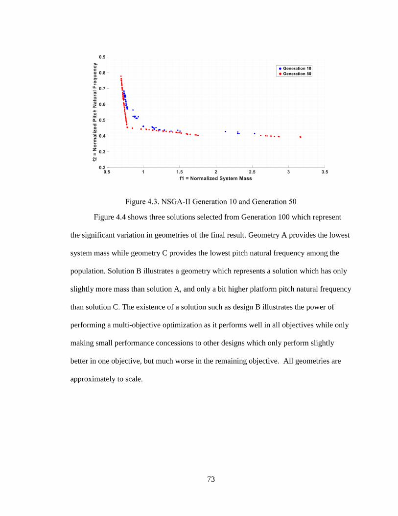
73

Figure 4.3. NSGA-II Generation 10 and Generation 50

Figure 4.4 shows three solutions selected from Generation 100 which represent

the significant variation in geometries of the final result. Geometry A provides the lowest

system mass while geometry C provides the lowest pitch natural frequency among the

population. Solution B illustrates a geometry which represents a solution which has only

slightly more mass than solution A, and only a bit higher platform pitch natural frequency

than solution C. The existence of a solution such as design B illustrates the power of

performing a multi-objective optimization as it performs well in all objectives while only

making small performance concessions to other designs which only perform slightly

better in one objective, but much worse in the remaining objective. All geometries are

approximately to scale.

74

Figure 4.4. NSGA-II Generation 100

Results (see Appendix B) from the NSGA-II run reveal a tendency for the optimal

moonpool dimension to be between 11.34 m and 44.0 m, these values being well within

the bounds set for this optimization variable. Additionally, the optimal hull width is very

close to the upper limit ranging from 54.0 m 58.1 m. The various combinations of these

dimensions force the width of the hull segment to stay between 7 m and 21.5 m. The

width of the heave plates along the Pareto front occupy the entirity of the allowable

range, with values of 0 m to 15 m. The hull height varies within the top two thirds of its

bounds, with the lowest value at 10.8 m and the highest value at the upper bound of 30 m.

The smallest normalized pitch frequency occurs when the heave plate width is towards its

upper bound at a value of approximately 15 m and the height of the hull is also near its

upper bound at approximately 30 m. By contrast, the smallest ratio of mass to the

nominal value is achieved when the heave plate width is approximately 0 m and the hull

height is approximately 10.9 m. This constitues a design with a height that is roughly one

third of the height for the optimal geometry for minimization of pitch natural frequency.

75

A tabulation of key characteristics of geometries from designs A, B, and C from

the Pareto front are given in Table 4.3. These results illustrate the true competing nature

of the two objective functions. Geometry A represents the minimum value of the mass

ratio objective while geometry C represents the minimum value of the pitch natural

frequency. Geometry B is a geometry which approximately represents the best case for

compromise between both objective functions. The values for 𝑃1, 𝑃2, and 𝑃4 for design

B are very similar to geometry A, but the value of 𝑃3 for geometry B is approximately

equal to the value of 𝑃3 for geometry C.

Table 4.3. Geometric properties from selected Pareto Front individuals

Geometry Nominal

Case

A B C

%

Change

%

Change

%

Change

𝑚𝑡𝑜𝑡/𝑚𝑛𝑜𝑚 1 0.61 -39.5 0.79 -21.2 3.22 222.0

𝜔𝑝𝑖𝑡𝑐ℎ/𝜔𝑝𝑖𝑡𝑐ℎ 𝑛𝑜𝑚 1 1.08 8.3 0.44 -55.8 0.39 -61.0

Moonpool

width (m) 30.9 43.78 41.7 42.45 37.4 11.34 -63.3

Hull width (m) 52.6 57.78 9.8 56.65 7.7 54.27 3.2

Heave plate

width (m) 0 0.01 100.0 14.98 100.0 14.98 100.0

Hull height (m) 14.7 10.86 -26.1 11.16 -24.1 29.67 101.8

Draft (m) 11.6 8.86 -23.6 9.09 -21.6 22.58 94.7

Hull mass (kg) 2.04 × 107 1.19 × 107 -41.7 1.21 × 107 -40.7 6.42 × 107 214.7

Heave natural

period (s) 10.1 8.31 -17.7 15.01 48.6 16.38 62.1

Pitch natural

period (s) 11.6 11.05 -4.7 27.09 133.6 30.72 164.9

76

4.5. Discussion

Based on the results of Table 4.3, the mass ratio and pitch natural frequency do

not have a significant dependence on the hull width (𝑃2) as this value is approximately

equal across all geometries. A smaller pitch natural frequency is achieved by increasing

the draft of the system and decreasing the width of the moonpool. An additional trend in

the results reveals that a relatively small sacrifice in the mass of the system can lead to a

significant reduction in the pitch natural frequency as shown in the difference between

designs A and B. This trend also exists in the other objective, as a small sacrifice in the

pitch natural frequency leads to significant improvement in reducing the mass of the

system when comparing designs C and B. Two of the three selected geometries make use

of a heave plate which the baseline case does not have. Even if the heave plate perimeter

is neglected the footprints of each of the selected geometries are larger than the baseline

case. The mass of the hull for the baseline case (2.04 × 107 kg) is larger than that of either

geometry A or geometry B, suggesting that despite their larger footprints they may be

able to provide some material savings. The mass of geometry C suggests that the small

advantage in pitch natural frequency would not be worth the sacrifice in mass.

Although these objective functions are important to the optimization of a wind

turbine hull, there are many other aspects to consider. This optimization assumes that

obtaining shorter platform pitch frequencies will yield better dynamic results, but this

does not necessarily reflect optimal designs which include the potential motion

reductions obtained from the moonpool effect for commonly occurring sea states with

wave periods between 5 and 20 seconds. Further exploration of geometric complexity

such as optimization of the shapes of the outer and moonpool perimeters could also have

77

an impact on the performance of the model. Another factor to look into would be the

positioning of the heave plates in the vertical direction as well as their orientation.

All calculations have assumed a smeared density of the hull. In practice the

density of the hull would not likely be uniform as the ballast (often water) would not

completely fill the cavity of the hull. Additionally, it would be possible to utilize an

active ballast system or to concentrate the ballast in particular regions within the hull to

reduce dynamic system responses. Structural considerations for the system would also

cause the need for supports to reduce the effective length of the structural members.

Material selection would further dictate the variability of the density of the hull. Overall,

the pitch performance and system can be improved with the selection of geometry B.

78

CHAPTER 5

CONCLUSIONS AND FUTURE WORK

5.1. Conclusions

A testing program was developed to validate the ability of ANSYS AQWA to

model annular FOWT hulls with moonpools. A 1/100th-scale model of an annular hull

was tested in the W2 basin which provided adequate results for comparison. Additionally,

the annular hull was put into context in a comparison with other commercially available

FOWT hull technologies.

Based on the results from this testing and validation effort, the following

observations were made:

ANSYS AQWA can adequately capture the impacts of moonpools in

numerical modeling provided that the lid damping factor is properly tuned

along with external damping

The RAO magnitudes exhibited by the annular hull are generally higher

than the results from the DeepCwind data set.

In this work, the general geometric shape was varied and the impacts on

hydrodynamic performance were evaluated. The results of this work illustrate that a

minimal sacrifice in the pitch RAO is likely worth the reduction in manufacturing and

transportation complexity offered by the annular square hull. The comparison of

geometric shape also confirmed that the moonpool does impact system motions in a

positive way and allows for significant material reduction when comparing with a barge

system for the support of a 6-MW turbine.

79

Further explorations in geometric variation led to an optimization of the square

annular hull which expressed the wide range of hull heights and heave plate addition

potential. Optimization results revealed that improvement in pitch performance from the

baseline case is reliant on the addition of heave plates. Interestingly the width of the

plates resulting from the optimization process exceeded the dimensions as described

when considering the 6-MW-scale Ideol model. In addition to the necessity of heave

plates for improved performance it was also noted that a significant increase in system

draft to optimize for pitch natural frequency is not worth the sacrifice in system mass.

5.2. Future Work

All portions of this work assume a solid hull with uniform density which is a

simplification when comparing to practical applications. Future work should include

considering the potential variability in material selection for the structure itself as well as

the ballast. Along with considering potential materials for the hull, the mooring method

should also be taken into account when evaluating system responses. A hull with a

catenary chain mooring system could experience significantly different mooring

stiffnesses from a taught synthetic system—either of which would provide more than the

zero magnitude pitch mooring stiffness case which is considered herein.

It is important to emphasize that this work only investigates unidirectional waves.

With the motion of the water in the moonpool highly dependent on the motion of the

water surrounding the hull the consideration of the multidirectional case would prove

crucial for further development. Waves have only been assumed to approach from the

direction perpendicular to the sides of the hull while interactions at an angle may have a

significant impact in the motions of the water in the moonpool.

80

The applications for the annular FOWT hull as studied are rather limited as

significant system responses are exhibited in the range of wave periods which represent

typical sea states. Fortunately, significant potential exists for hull improvement for

seaworthiness. Variability of geometry both along the perimeter of the hull as well as the

perimeter of the moonpool could prove beneficial. Along with this, considerations for

heave plate orientation including vertical positioning as well as the potential for angled

heave plates may prove interesting. In these explorations it is important to remember that

the FOWT industry is constantly evolving to support larger wind turbines so any solution

should take scalability into consideration.

81

REFERENCES

Aalbers, A. B. (1984). THE WATER MOTIONS IN A MOONPOOL. Ocean Engng,

11(6), 55–579. Retrieved from https://ac-els-cdn-

com.prxy4.ursus.maine.edu/0029801884900015/1-s2.0-0029801884900015-

main.pdf?_tid=f4ca800a-a842-11e7-be12-

00000aab0f01&acdnat=1507039298_a8126e6063a77052a965a1a0545685b0

ANSYS Inc. (2013a). Aqwa Theory Manual, 15317(November), 724–746.

ANSYS Inc. (2013b). Aqwa User’s Manual. Canonsburg, PA: ANSYS, Inc.

Beyer, F., Choisnet, T., Kretschmer, M., & Cheng, P. W. (2015). Coupled MBS-CFD

Simulation of the IDEOL Floating Offshore Wind Turbine Foundation Compared to

Wave Tank Model Test Data. In International and Polar Engineering Conference.

International Society of Offshore and Polar Engineers. Retrieved from https://www-

onepetro-org.prxy4.ursus.maine.edu/download/conference-paper/ISOPE-I-15-

272?id=conference-paper%2FISOPE-I-15-272

Chakrabarti, S. K. (1994). Advanced Series on Ocean Engineering, Volume 9: Offshore

Structure modeling. World Scientific.

Coulling, A. J., Goupee, A. J., Robertson, A. N., & Jonkman, J. M. (2013).

IMPORTANCE OF SECOND-ORDER DIFFERENCE-FREQUENCY WAVE-

DIFFRACTION FORCES IN THE VALIDATION OF A FAST SEMI-

SUBMERSIBLE FLOATING WIND TURBINE MODEL, 1–10.

Dagher, H., Viselli, A., Goupee, A., Kimball, R., & Allen, C. (2017). The VolturnUS 1:8

Floating Wind Turbine: Design, Construction, Deployment, Testing, Retrieval, and

Inspection of the First Grid-Connected Offshore Wind Turbine in US. Retrieved

from https://www.osti.gov/servlets/purl/1375022

Deb, K., Agrawal, S., Pratap, A., & Meyarivan, T. (2000). A Fast Elitist Non-Dominated

Sorting Genetic Algorithm for Multi-Objective Optimization: NSGA-II. Retrieved

from http://www.iitk.ac.in/kangal

Det Norske Veritas. (2014). Recommended Practice DNV-RP-C205: Environmental

Conditions and Environmental Loads. Retrieved from www.dnvgl.com.

Dvorak, P. (2015). Denmark’s Henrik Stiesdal unveils open-sourced floating offshore

platform. Can you improve on it? Retrieved May 23, 2018, from

https://www.windpowerengineering.com/business-news-projects/denmarks-henrik-

stiesdal-unveils-open-sourced-floating-offshore-platform-can-you-improve-on-it/

Energias de Portugal. (2018). WindFloat | edp.com. Retrieved January 29, 2019, from

https://www.edp.com/en/windfloat

82

EOLFI. (2018). Les Eoliennes Flottantes de Groix &amp; Belle-Ile Dossier

D’information Septembre 2018. Retrieved from http://eoliennes-groix-belle-

ile.com/wp-content/uploads/2018/10/eolfi_plaquette-12pages_13_bd.pdf

Equinor. (2018). Hywind - leading floating offshore wind solution - equinor.com.

Retrieved May 29, 2018, from https://www.equinor.com/en/what-we-do/hywind-

where-the-wind-takes-us.html

Fukushima Offshore Wind Consortium. (2013). Fukushima Floating Offshore Wind

Farm Demonstration Project (Fukushima FORWARD). Retrieved from

http://www.fukushima-forward.jp/english/pdf/pamphlet3.pdf

Fukushima Offshore Wind Consortium. (2016a). 5MW wind turbine on Fukushima

Hamakaze being towed to off Fukushima coast／News／Fukushima Offshore Wind

Consortium. Retrieved May 23, 2018, from http://www.fukushima-

forward.jp/english/news_release/news160801.html

Fukushima Offshore Wind Consortium. (2016b). Fukushima Floating Offshore Wind

Farm Demonstration Project (Fukushima FORWARD) -Construction of Phase II.

Retrieved from http://www.fukushima-forward.jp

Gaillarde, G., & Cotteleer, A. (2005). WATER MOTION IN MOONPOOLS

EMPIRICAL AND THEORETICAL APPROACH Anke COTTELEER. Maritime

Research Institute, Netherlands. Retrieved from www.marin.nl

GICON-SOF. (2015). Media: Das GICON®-SOF Schwimmendes Offshorefundament.

Retrieved January 7, 2019, from http://www.gicon-sof.de/en/media.html

GICON-SOF. (2018). Technical Solution: Das GICON®-SOF Schwimmendes

Offshorefundament. Retrieved January 7, 2019, from http://www.gicon-

sof.de/en/technical-solution.html

Goupee, A. J., Koo, B. J., Kimball, R. W., Lambrakos, K. F., & Dagher, H. J. (2014).

Experimental Comparison of Three Floating Wind Turbine Concepts. Journal of

Offshore Mechanics and Arctic Engineering, 136(2), 020906.

https://doi.org/10.1115/1.4025804

Goupee, A. J., & Vel, S. S. (2007). Multi-objective optimization of functionally graded

materials with temperature-dependent material properties. Materials & Design,

28(6), 1861–1879. https://doi.org/10.1016/J.MATDES.2006.04.013

Greenovate! Europe EEIG. (2013). Floating offshore wind combining cost-

competitiveness and high local content: Demonstration and benchmarking of a

floating wind turbine system for power generation in Atlantic deep waters. Retrieved

from http://ideol-offshore.com/sites/default/files/pdf/plaquette_floatgen-bd.pdf

83

Großmann, J., Dahlhaus, F., Adam, F., & Schuldt, B. (2014). The GICON ®-TLP for

wind turbines: Experimental Studies and numerical Modelling of structural

Behavior of a Scaled Modular TLP Structure for Offshore Wind turbines. Retrieved

from

https://www.sintef.no/globalassets/project/deepwind2014/presentations/e/adam-

f_gicon.pdf

GustoMSC. (2019). TRI-FLOATER FLOATING OFFSHORE WIND TURBINE

FOUNDATION. Retrieved from www.gustomsc.com

Halkyard, J. (2013). Design and Analysis of Floating Structures. (S. Chakrabarti, Ed.)

(3rd, Versi ed.). Houston, TX: Elsevier Science.

Hermans, K. W., Peeringa, J. M., & Verbruggen, T. (2016). The influence of offshore

floating foundations to the wind turbine generator A study using aNySIMPHATAS.

Retrieved from https://www.ecn.nl/publications/PdfFetch.aspx?nr=ECN-E--16-032

Huijs, F., de Bruijn, R., & Savenije, F. (2014). Concept Design Verification of a Semi-

submersible Floating Wind Turbine Using Coupled Simulations. Energy Procedia,

53, 2–12. https://doi.org/10.1016/J.EGYPRO.2014.07.210

Ideol. (2018a). Floatgen is installed ! | Ideol. Retrieved January 7, 2019, from

https://www.ideol-offshore.com/en/actualites/floatgen-installed

Ideol. (2018b). Floating wind turbine solution | Japn offshore wind. Retrieved January 29,

2019, from https://www.ideol-offshore.com/en/japanese-demonstrator

Ideol. (2018c). Ideol floating platform | offshore wind power. Retrieved December 28,

2018, from https://www.ideol-offshore.com/en/floatgen-demonstrator

Jonkman, J. M. (2007). Dynamics Modeling and Loads Analysis of an Offshore Floating

Wind Turbine Dynamics Modeling and Loads Analysis of an Offshore Floating

Wind Turbine, (November).

Koo, B. J., Goupee, A. J., Kimball, R. W., & Lambrakos, K. F. (2014). Model Tests for a

Floating Wind Turbine on Three Different Floaters. Journal of Offshore Mechanics

and Arctic Engineering, 136(2), 020907. https://doi.org/10.1115/1.4024711

Kurtenbachap, E. (2013). Japan launches full-size floating wind turbine near Fukushima.

Portland Press Herald. Retrieved from

https://www.pressherald.com/2013/11/11/japan_launches_full-

size_floating_wind_turbine_near_fukushima/

84

Lauridsen, L. (2017). Millioner til Stiesdals flydende vindmølle-fundament | TV

MIDTVEST. Retrieved May 23, 2018, from

https://www.tvmidtvest.dk/artikel/millioner-til-stiesdals-flydende-vindmoelle-

fundament

LHEEA Centrale Nantes. (2018). FLOATGEN. cnrs. Retrieved from https://lheea.ec-

nantes.fr/partnerships-and-projects/research-projects/floatgen-201151.kjsp

Liu, Y., Li, S., Yi, Q., & Chen, D. (2016). Developments in semi-submersible floating

foundations supporting wind turbines: A comprehensive review. Renewable and

Sustainable Energy Reviews, 60, 433–449.

https://doi.org/10.1016/J.RSER.2016.01.109

Manzanas Ochagavia, R., Pascual Vergara Daniel Castell, J., Rodriguez Tsouroukdissian

Jaco Korbijn, A., Bolleman Francisco J Huera-Huarte, N. C., Schuon, F., Ugarte

Johan Sandberg Vincent de Laleu, A., … Wilkes, J. (2013). Deep Water The next

step for offshore wind energy. (J. S. and Sarah Azau, Stéphane Bourgeois, Zoë

Casey, Jacopo Moccia, Vilma Radvilaite & Justin Wilkes (EWEA), Eds.). Retrieved

from www.ewea.org/report/deep-water

Mitsubishi Corporation. (2015). Fukushima Experimental Offshore Floating Wind Farm

Project: Second Phase Update. Retrieved January 7, 2019, from

https://www.mitsubishicorp.com/jp/en/pr/archive/2015/html/0000027886.html

Molin, B. (2001). On the piston and sloshing modes in moonpools. J. Fluid Mech, 430,

27–50. https://doi.org/10.1017/S0022112000002871

Musial, W. (2018). Offshore Wind Resource, Cost, and Economic Potential in the State of

Maine. Retrieved from https://www.nrel.gov/docs/fy18osti/70907.pdf

Musial, W., Heimiller, D., Beiter, P., Scott, G., & Draxl, C. (2016). 2016 Offshore Wind

Energy Resource Assessment for the United States. Retrieved from

www.nrel.gov/publications.

offshoreWIND.biz. (2016a). Fukushima Hamakaze Nearing Completion | Offshore Wind.

Retrieved May 23, 2018, from

https://www.offshorewind.biz/2016/05/06/fukushima-hamakaze-nearing-

completion/

offshoreWIND.biz. (2016b). Fukushima Hamakaze Spar Tilts Back Into Position |

Offshore Wind. Retrieved May 23, 2018, from

https://www.offshorewind.biz/2016/05/17/fukushima-hamakaze-spar-tilts-back-into-

position/

Principle. (2014). WindFloat Pacific OSW Project. Retrieved from

https://www.boem.gov/NREL-WindFloat-Pacific-OSW-Project/

85

Robertson, A. N., & Jonkman, J. M. (2011). Loads Analysis of Several Offshore Floating

Wind Turbine Concepts. Retrieved from www.deepcwind.org

Sclavounos, P. (2008). Floating Offshore Wind Turbines. Marine Technology Society

Journal, 42(2), 39–43. https://doi.org/10.4031/002533208786829151

Stehly, T., Beiter, P., Heimiller, D., & Scott, G. (2017). 2017 Cost of Wind Energy

Review. Retrieved from www.nrel.gov/publications.

WINDExchange. (2017). WINDExchange: U.S. Wind Power Resource at 100-meter Hub

Height. Retrieved August 22, 2018, from https://windexchange.energy.gov/maps-

data/324

86

APPENDIX A: OPTIMIZATION MATLAB FUNCTIONS

%H. Allen % Last updated 05/01/2019

function [obj1,obj2,c, kP, g1, g2, g3, g4] = myfuns(p) %% Constants g = 9.81; %%m/s^2 dh2o = 1025; %desity of sea water kg/m^3 dhull = 768.03;%%density of hull kg/m^3 dplate = 1895;%%density of heave plate kg/m^3 tplate = 0.457;%%heave plate thickness (~1.5ft) mturb = 438*10^3; %%turbine mass, kg mtow0 = 517.371*10^3; %%tower mass, kg %mtt = mturb+mtow; %%Mass of turbine and tower, metric tons towhgt0 = 83.5; %nominal tower height, m towcgz0 = 36.3463; %nominal tower cg from base wind = 846*10^3; %%Design case wind load, N windarm = 100; %%moment arm for wind turbine, m windmom = wind*windarm; %%wind moment mnom = 21341.181*10^3; %%nominal mass of hull, turbine, tower, ballast wheavenom = 0.625; %%nominal heave natural frequency, rad/s FIX!!! wpitchnom = 0.525; %%nominal pitch natural frequency, rad/s FIX!!! %%optimization, previously determined, kg %% Design variable dependent calculations: p is the vector of %design variables moonside = p(1);%%p1=mooonpool side length hullside = p(2);%%p2=hull body side length platew = p(3);%%p3=heave plate width hullh = p(4); %%p4=hull height

Awp = (hullside^2-moonside^2);%%waterplane area, m vhull = Awp*hullh; %%hull total volume, m^3 mhull = (vhull*dhull); %%mass of hull w/ballast thull = (hullside-moonside)/2; %%thickness of hull

vplate = ((hullside+2*platew)^2-(hullside^2))*tplate; %plate volume mplate = vplate*dplate; %%plate mass

%m = mhull+mplate+mtt; %%total system mass, kg

%%draft based on mass of system draft = (mhull+mturb+mtow0*((100-hullh)/towhgt0))/... ((-mtow0/towhgt0)+dh2o*Awp);%draf, m vsub = draft*Awp+vplate; %%submerged volume towhgt = 100-(hullh-draft); %height of tower maintaining hub height of

100m towcgz = towcgz0*(towhgt/towhgt0); %tower center of gravity mtow = mtow0*(towhgt/towhgt0); %mass of tower mtt = mturb+mtow; %% mass of turbine and tower, kg m = mhull+mplate+mtt; %%total system mass, kg

%%CG in reference to water line at aft, left corner (behind turbine)

87

CGx = (hullside)/2; %location of center of gravity in surge direction,

m CGy = CGx; %location of center of gravity in sway direction, m %location of center of gravity in heave direction, m CGz = ((mhull*((hullh/2)-draft))+(mplate*-(draft-(tplate/2)))... +mturb*(100)+mtow*(towcgz+(hullh-draft)))/m;

%%Waterplane stiffness (P=pitch, H=heave) kP = (dh2o*g*(hullside^4-moonside^4)/12)+(dh2o*g*vsub*-draft/2)-

(m*g*CGz);%Nm/rad kH = (dh2o*g*(hullside^2-moonside^2)); %N/m

thetaP = (windmom/kP)*(360/2*pi); %%pitch rotation, degrees

%%Pitch Inertia (values for added mass calculated later on) IPplate =

(mplate/2)*((((hullside+2*platew)^2)/12)+(((hullside+platew)/2)^2));

%plate inertia IPhull = (mhull - mtt)/2*(((hullside^2)/12)+((hullside-thull)/2)^2);

%hull inertia %Inertia due to counterweight to balance turbine and tower, %positioned in hull horizontally 180 degrees from turbine and tower. IPtthull = mtt*((hullside/2)^2); %turbine and tower inertia, assuming cg is at MWL IPtt = (mturb*(100^2)+mtow*((towcgz+(hullh-draft))^2)); IP = IPplate+IPhull+IPtthull+IPtt; %% Constraint functions. All nom values are based on the nominal 6MW

hull %%g1 constraint of width of hull segment tnom = 10.823; %%nominal thickness of hull segment, m if thull<=7 g1 = (7-thull)/tnom; else g1 = 0; end

%%g2 drives draft to be less than hull height (bouyancy) dnom = 11.596; %%m if draft>=hullh g2 = (draft-hullh)/dnom; else g2 = 0; end

%%g3 drives pitch stiffness to be as good or better than the nominal

case kPnom = 4630990675; %%Nm/rad if kP<=0 g3 = -kP/kPnom; else g3 = 0; end

%%g4 drives pitch angular displacement to be less than or equal to the

88

%%nominal case thetaPnom = 0.018269*(360/2*pi); %%nominal pitch angular disp, deg thetamax = 10; %deg if thetaP>=thetamax g4 = (thetaP-thetamax)/thetamax; else g4 = 0; end

%%g5 (added 3-5-19) drives the freeboard of the hull to be 2 m or %geater to help reduce greenwater in day-to-day conditions minfreeb = 2; % minimum freeboard, m freeb = hullh-draft; if freeb<=minfreeb g5 = (minfreeb-freeb)/minfreeb; else g5 = 0; end

c = g1+g2+g3+g4+g5;

%% Calculate objective functions if (c <= 0)

%%added masses in heave based on DNV-RP-C205 2-D guidelines %%HEAVE FROM HULL%% ratio = ((hullside-moonside)/2)/draft; if ratio>10.5 CA = 1; elseif (ratio>=7.5) && (ratio<=10.5) CA = 1.14; elseif (ratio>=3) && (ratio<7.5) CA = 1.21; elseif (ratio>=1.5) && (ratio<3) CA = 1.36; elseif (ratio>=0.75) && (ratio<1.5) CA = 1.51; elseif (ratio>=0.35) && (ratio<0.75) CA = 1.70; elseif (ratio>=0.15) && (ratio<0.35) CA = 1.98; % elseif (ratio>=.085) && (ratio<0.15) % CA = 2.23; elseif (ratio == 0) CA = 0; else CA = 2.23; end AR = pi*(((hullside-moonside)/4)^2); %reference area as defined by

C205 L = 4*(hullside-((hullside-moonside)/2)); %sidelengths relevant to

hull heave maddedHh = dh2o*CA*AR; %hull heave added mass per length maddedHhtot = L*dh2o*CA*AR;

%%HEAVE FROM HEAVE PLATES%%

89

ratio = platew/tplate; if ratio>10.5 CA = 1; elseif (ratio>=7.5) && (ratio<=10.5) CA = 1.14; elseif (ratio>=3) && (ratio<7.5) CA = 1.21; elseif (ratio>=1.5) && (ratio<3) CA = 1.36; elseif (ratio>=0.75) && (ratio<1.5) CA = 1.51; elseif (ratio>=0.35) && (ratio<0.75) CA = 1.70; elseif (ratio>=0.15) && (ratio<0.35) CA = 1.98; else CA = 2.23; end AR = pi*(platew/2)^2; L = 4*(hullside+platew);%sidelengths relevant to plate heave maddedHp = dh2o*CA*AR; %plate heave added mass per unit length maddedHptot = L*dh2o*CA*AR;%updated 1-25 to reflect 4 plate

segments

maddedHtot= maddedHhtot+maddedHptot; %total added mass in heave, kg wheave = sqrt(kH/(m+maddedHtot));%heave natural frequency critdamp =2*sqrt(kH*(m+maddedHtot)); %critical damping critdampH = 0.1*critdamp; %10% of critical damping

%% added mass inertia in pitch based on heave added mass from % DNV-RP-C205 %FROM HULL% IaddedPh = (2*maddedHh*hullside*(((hullside/2)-

(thull/2))^2))+(2*(1/12)*maddedHh*moonside*(moonside^2));%%added

inertia (kgm^2)from hull %FROM PLATE% IaddedPp =

(2*maddedHp*(hullside+2*platew)*((hullside+2*platew)/2)^2)+(2*(1/12)*ma

ddedHp*(hullside+2*platew)*((hullside+2*platew)^2));; %%pitch added

inertia from plates

IaddedP = IaddedPh+IaddedPp;%total pitch inertia wpitch = sqrt(kP/(IP+IaddedP)); %wpitch = 2*pi/wpitch; %%pitch natural period, s

%Objective Functions obj1 = -m/mnom; %normalized mass, trying to minimize

obj2 = -sqrt(kP/(IP+IaddedP))/wpitchnom; %%normalized pitch natural frequency, trying to minimize else obj1 = -(5+c); obj2 = -(5+c); end

%Main Multi-Objective Genetic Algorithm (MOGA) Input Page

90

%Andrew Goupee %Last modified: 12-2-04

%This algorithm utilizes an elitist multi-objective genetic algorithm

with %crowded tournament selection and a constrained non-domination sorting %routine. Details of these operators can be viewed in Deb's book. %This m-file allows one to select the values of various MOGA parameters

used %in searching for the pareto-optimal front (searching for maximums)

under %linear and/or %nonlinear constraints. Recommended values of the GA

parameters %are given in various works by Deb. The parameters to be chosen are as %follows:

%MOGA parameters to be chosen: %max_gen - the number of generations until termination %n_pop - size of GA population (must be an even number) %n_genes - number of genes in an individuals chromosome %ub_1 - vector of upper bounds on genes (design parameters) for initial % population, dimensions of 1 row x n_genes columns %lb_1 - vector of lower bounds on genes (design parameters) for initial % population, dimensions of 1 row x n_genes columns %ub_2 - vector of upper bounds on genes (design parameters) for all % populations after initial, dimensions of 1 row x n_genes columns %lb_2 - vector of lower bounds on genes (design parameters) for all % populations after initial, dimensions of 1 row x n_genes columns %pc - probability of crossover per pair of parents %pcg - probability of crossover per gene %nc - crossover strength parameter (smaller values increase strength) %pm - probability of mutation per individual %pmg - probability of of mutation per gene %nm - mutation strength parameter (smaller values increase strength) %drop - overall percent reduction in chosen parameters (for those that % apply) calculated during dynamic parameter alteration %dyn - strength parameter for dynamic alteration scheme (larger values % reduce parameters by percent alloted in 'drop' quicker) %objective1, objective2 - character strings containing the names of the % two objective functions to be maximized %constraint - character string containing the name of the constraint % function

%Output %A plot of the fitness functions

clear all;

%Select GA paramters: max_gen = 100; %Number of generations

n_pop = 100; %Number of members of each population

n_genes = 4; %Number of variables to be manipulated

91

ub_1 = [60 74 15 30]; %Upper bounds on genes in meters, applied

throughout

lb_1 = [10 30 0 5]; %Lower bounds on genes in meters, applied

throughout

ub_2 = ub_1;

lb_2 = lb_1;

pc = 1;

pcg = .5;

nc = 2;

pm = .1;

pmg = .5;

nm = 2;

plotbounds=[0 2.5 0 1];

track=0;

minplot=1;

%Provide objective and constraint function name objective = 'myfuns';

%Perform GA search and optimization [population]=MOGAmain(max_gen,n_pop,n_genes,ub_1,lb_1,ub_2,lb_2,... pc,pcg,nc,pm,pmg,nm,objective,... plotbounds,track,minplot);

92

function [population] =

MOGAmainMOGAmain(max_gen,n_pop,n_genes,ub_1,lb_1,... ub_2,lb_2,pc,pcg,nc,pm,pmg,nm,objective,... plotbounds,track,minplot) %Main multi-objective genetic algorithm program %Andrew Goupee %Last modified: 12-02-4

%Initialize generation number, corresponding generation generation = 0; [population] = create_population(n_pop,n_genes,ub_1,lb_1,objective);

pause(0.01); figure(1); clf; hold on; axis(plotbounds); title('Generation 0'); if (minplot == 1) for i=1:n_pop plot(-population(i,4),-population(i,5),'k.'); if (track == 1) stores(i,2*generation+1)=-population(i,4); stores(i,2*generation+2)=-population(i,5); end; end; else for i=1:n_pop plot(population(i,4),population(i,5),'k.'); if (track == 1) stores(i,2*generation+1)=population(i,4); stores(i,2*generation+2)=population(i,5); end; end; end; pause(0.01);

%Begin looping through generations generation = 1; while (generation <= max_gen)

%Perform tournament selection [population] = matingpool(population);

%Perform crossover and mutation to create 2N mating pool [dpop] = hankypanky(population,pc,pcg,pm,pmg,ub_2,lb_2,... nc,nm,objective);

%Perform elitist function population = dpop(1:n_pop,:);

pause(0.01); figure(1); if (track == 0) clf;

93

hold on; axis(plotbounds); title(['Generation ',num2str(generation)]); if (minplot == 1) for i=1:n_pop plot(-population(i,4),-population(i,5),'k.'); end; else for i=1:n_pop plot(population(i,4),population(i,5),'k.'); end; end; else clf; hold on; axis(plotbounds); title(['Generation ',num2str(generation)]); if (minplot == 1) for i=1:n_pop for j=1:generation plot(stores(i,2*j-1),stores(i,2*j),'mo'); plot(stores(i,2*j-1),stores(i,2*j),'mo'); end; end; for i=1:n_pop plot(-population(i,4),-population(i,5),'k.'); stores(i,2*generation+1)=-population(i,4); stores(i,2*generation+2)=-population(i,5); end; else for i=1:n_pop for j=1:generation plot(stores(i,2*j-1),stores(i,2*j),'mo'); plot(stores(i,2*j-1),stores(i,2*j),'mo'); end; end; for i=1:n_pop plot(population(i,4),population(i,5),'k.'); stores(i,2*generation+1)=population(i,4); stores(i,2*generation+2)=population(i,5); end; end; end; pause(0.01);

%Count up generation generation = generation + 1;

%Save GA information save moga_info;

population(:,4:5) end;

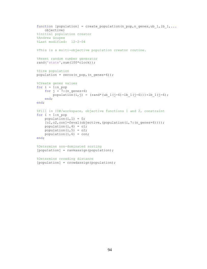
94

function [population] = create_population(n_pop,n_genes,ub_1,lb_1,... objective) %Initial population creator %Andrew Goupee %Last modified: 12-2-04

%This is a multi-objective population creator routine.

%Reset random number generator rand('state',sum(100*clock));

%Size population population = zeros(n_pop,(n_genes+6));

%Create genes values for i = 1:n_pop for j = 7:(n_genes+6) population(i,j) = (rand*(ub_1(j-6)-lb_1(j-6)))+lb_1(j-6); end; end;

%Fill in ID#/workspace, objective functions 1 and 2, constraint for i = 1:n_pop population(i,1) = 0; [o1,o2,con]=feval(objective,(population(i,7:(n_genes+6)))); population(i,4) = o1; population(i,5) = o2; population(i,6) = con; end;

%Determine non-dominated sorting [population] = rankassign(population);

%Determine crowding distance [population] = crowdassign(population);

95

function [matepool] = matingpool(population) %This creates a mating pool from a population %Andrew Goupee %12-03-04

population(:,1)=0; [n_pop,len]=size(population); matepool=zeros(n_pop,len);

for i=1:n_pop

%Select individual 1 flag=0; while (flag < 1) no_1=random(n_pop); if (population(no_1,1) < 2) dude1=population(no_1,:); flag=1; population(no_1,1)=population(no_1,1)+1; end; end;

%Select individual 2 flag=0; while(flag < 1) no_2=random(n_pop); if (population(no_2,1) < 2) dude2=population(no_2,:); flag=1; population(no_2,1)=population(no_2,1)+1; end; end;

%Conduct tournament if (dude1(1,2) < dude2(1,2)) matepool(i,:)=dude1; elseif (dude2(1,2) < dude1(1,2)) matepool(i,:)=dude2; else if (dude1(1,3) > dude2(1,3)) matepool(i,:)=dude1; elseif (dude2(1,3) > dude1(1,3)) matepool(i,:)=dude2; else matepool(i,:)=dude1; end; end;

end;

matepool(:,1)=0;

96

function [dpop] = crossmutate(population,pc,pcg,pm,pmg,ub_2,lb_2,... nc,nm,objective) %This function performs crossover, mutation, makes 2N population %Andrew Goupee %Last modified: 12-03-04

population(:,1)=0; [n_pop,len]=size(population); dpop=zeros(2*n_pop,len); dpop(1:n_pop,:)=population; dpop(:,1:3)=0; n_genes=len-6;

%Make children for i=1:(n_pop/2)

checks=[0 0];

%Pick out mom flag=0; while (flag < 1) no_1=random(n_pop); if (dpop(no_1,1) < 1) parent_1 = dpop(no_1,:); dpop(no_1,1)=1; flag=1; end end

%pick out dad flag=0; while (flag < 1) no_2=random(n_pop); if (dpop(no_2,1) < 1) parent_2 = dpop(no_2,:); dpop(no_2,1)=1;

flag=1; end end

%Perform crossover if necessary if (rand <= pc)

checks = [1 1];

%Loop through genes for j = 7:(n_genes+6)

%Determine if genes are to be crossed if (rand <= pcg)

%Perform crossover if (parent_1(1,j) < parent_2(1,j)) x1 = parent_1(1,j);

97

x2 = parent_2(1,j); else x1 = parent_2(1,j); x2 = parent_1(1,j); end

if (x2 == x1) difference = .01; else difference = x2 - x1; end

beta = 1 + (2/difference)*... (min([(x1-lb_2(1,j-6)),(ub_2(1,j-6)-x2)]));

alpha = 2 - beta^(-(nc+1));

u = rand; if (u <= (1/alpha)) beta_bar = (alpha*u)^(1/(nc+1)); else beta_bar = (1/(2-alpha*u))^(1/(nc+1)); end

y1 = 0.5*((x1+x2) - beta_bar*(x2-x1)); y2 = 0.5*((x1+x2) + beta_bar*(x2-x1));

if (parent_1(1,j) < parent_2(1,j)) child_1(1,j) = y1; child_2(1,j) = y2; else child_1(1,j) = y2; child_2(1,j) = y1; end else child_1(1,j) = parent_1(1,j); child_2(1,j) = parent_2(1,j); end end else %Just copy over parents to children if no crossover at all child_1 = parent_1; child_2 = parent_2; end %Mutate if necessary %child_1 if (rand < pm)

checks(1,1) = 1;

%Erase fitness and constraint violation child_1(1,1:6)=0;

%Loop through genes for j=7:(n_genes+6)

98

%Determine if gene is to be mutated if (rand < pmg)

%Perform mutation x = child_1(1,j);

%Calculate gap if (ub_2(1,j-6) == lb_2(1,j-6)) gap = 1; else gap = ub_2(1,j-6)-lb_2(1,j-6); end

delta = (min([(x-lb_2(1,j-6)),(ub_2(1,j-6)-x)]))/... gap;

u = rand; if (u <= 0.5) delta_bar = ((2*u+(1-2*u)*((1-delta)^(nm+1)))... ^(1/(nm+1))) - 1; else delta_bar = 1 - (2*(1-u)+2*(u-0.5)*((1-

delta)^(nm+1)))... ^(1/(nm+1)); end

y = x + delta_bar*(ub_2(1,j-6) - lb_2(1,j-6));

child_1(1,j) = y; end end end

%child_2 if (rand < pm)

checks(1,2) = 1;

%Erase fitness and constraint violation child_2(1,1:6)=0;

%Loop through genes for j=7:(n_genes+6)

%Determine if gene is to be mutated if (rand < pmg)

%Perform mutation x = child_2(1,j);

%Calculate gap if (ub_2(1,j-6) == lb_2(1,j-6)) gap = 1;

99

else gap = ub_2(1,j-6)-lb_2(1,j-6); end

delta = (min([(x-lb_2(1,j-6)),(ub_2(1,j-6)-x)]))/... gap;

u = rand; if (u <= 0.5) delta_bar = ((2*u+(1-2*u)*((1-delta)^(nm+1)))... ^(1/(nm+1))) - 1; else delta_bar = 1 - (2*(1-u)+2*(u-0.5)*((1-

delta)^(nm+1)))... ^(1/(nm+1)); end

y = x + delta_bar*(ub_2(1,j-6) - lb_2(1,j-6));

child_2(1,j) = y; end end end

dpop(((2*i)-1)+n_pop,:)=child_1; dpop(2*i+n_pop,:)=child_2;

%Evaluate objective function if needed if (checks(1,1) == 0) dpop(((2*i)-1)+n_pop,4)=parent_1(1,4); dpop(((2*i)-1)+n_pop,5)=parent_1(1,5); dpop(((2*i)-1)+n_pop,6)=parent_1(1,6); else [o1,o2,con]=feval(objective,(child_1(1,7:(n_genes+6)))); dpop(((2*i)-1)+n_pop,4)=o1; dpop(((2*i)-1)+n_pop,5)=o2; dpop(((2*i)-1)+n_pop,6)=con; end

if (checks(1,2) == 0) dpop(2*i+n_pop,4)=parent_2(1,4); dpop(2*i+n_pop,5)=parent_2(1,5); dpop(2*i+n_pop,6)=parent_2(1,6); else [o1,o2,con]=feval(objective,(child_2(1,7:(n_genes+6)))); dpop(2*i+n_pop,4)=o1; dpop(2*i+n_pop,5)=o2; dpop(2*i+n_pop,6)=con; end end %Rank assign [dpop] = rankassign(dpop);

%Crowd assign [dpop] = crowdassign(dpop)

100

function [popranked] = rankassign(population) %Rank assignment routine %Andrew Goupee %Last modified: 12-3-04 %This routine takes in a population of size n_pop and %finds their non-dominant rank and assigns it

[n_pop,len]=size(population); n_genes=len-6;

remainder=population; remainder(1:n_pop,1:3)=0; [n_rem,soup]=size(remainder); population=zeros(n_pop,(n_genes+6));

count=1; rank=1;

while (count <= n_pop)

for i=1:n_rem for j=1:n_rem [flag]=dominate(remainder(j,:),remainder(i,:)); remainder(i,1)=remainder(i,1)+flag; end; end;

rcount=1;

for i=1:n_rem if (remainder(i,1) == 0) population(count,:)=remainder(i,:); population(count,2)=rank; count=count+1; else remainder2(rcount,:)=remainder(i,:); rcount=rcount+1; end; end;

if (rcount > 1) remainder2=remainder2(1:rcount-1,:); else remainder2=remainder2(1,:); end;

[n_rem,soup]=size(remainder2); remainder=remainder2; remainder(:,1)=0; rank=rank+1;

end;

popranked=population(1:n_pop,:); function [popcrowd] = crowdassign(population)

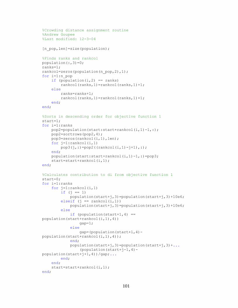
101

%Crowding distance assignment routine %Andrew Goupee %Last modified: 12-3-04

[n_pop,len]=size(population);

%Finds ranks and rankcol population(:,3)=0; ranks=1; rankcol=zeros(population(n_pop,2),1); for i=1:n_pop if (population(i,2) == ranks) rankcol(ranks,1)=rankcol(ranks,1)+1; else ranks=ranks+1; rankcol(ranks,1)=rankcol(ranks,1)+1; end; end;

%Sorts in descending order for objective function 1 start=1; for i=1:ranks pop2=population(start:start+rankcol(i,1)-1,:); pop2=sortrows(pop2,4); pop3=zeros(rankcol(i,1),len); for j=1:rankcol(i,1) pop3(j,:)=pop2((rankcol(i,1)-j+1),:); end; population(start:start+rankcol(i,1)-1,:)=pop3; start=start+rankcol(i,1); end;

%Calculates contribution to di from objective function 1 start=0; for i=1:ranks for j=1:rankcol(i,1) if (j == 1) population(start+j,3)=population(start+j,3)+10e6; elseif (j == rankcol(i,1)) population(start+j,3)=population(start+j,3)+10e6; else if (population(start+1,4) ==

population(start+rankcol(i,1),4)) gap=1; else gap=(population(start+1,4)-

population(start+rankcol(i,1),4)); end; population(start+j,3)=population(start+j,3)+... (population(start+j-1,4)-

population(start+j+1,4))/gap;... end; end; start=start+rankcol(i,1); end;

102

%Sorts in descending order for objective function 2 start=1; for i=1:ranks pop2=population(start:start+rankcol(i,1)-1,:); pop2=sortrows(pop2,5); pop3=zeros(rankcol(i,1),len); for j=1:rankcol(i,1) pop3(j,:)=pop2((rankcol(i,1)-j+1),:); end; population(start:start+rankcol(i,1)-1,:)=pop3; start=start+rankcol(i,1); end;

%Calculates contribution to di from objective function 2 start=0; for i=1:ranks for j=1:rankcol(i,1) if (j == 1) population(start+j,3)=population(start+j,3)+10e6; elseif (j == rankcol(i,1)) population(start+j,3)=population(start+j,3)+10e6; else if (population(start+1,5) ==

population(start+rankcol(i,1),5)) gap=1; else gap=(population(start+1,5)-

population(start+rankcol(i,1),5)); end; population(start+j,3)=population(start+j,3)+... (population(start+j-1,5)-

population(start+j+1,5))/gap;... end; end; start=start+rankcol(i,1); end;

%Sorts by crowding distance in descending order start=1; for i=1:ranks pop2=population(start:start+rankcol(i,1)-1,:); pop2=sortrows(pop2,3); pop3=zeros(rankcol(i,1),len); for j=1:rankcol(i,1) pop3(j,:)=pop2((rankcol(i,1)-j+1),:); end; population(start:start+rankcol(i,1)-1,:)=pop3; start=start+rankcol(i,1); end;

popcrowd=population;

103

function [number] = random(n) %Random number generator %Andrew Goupee %Last modified: 4-21-04

%This function generates a random integer between 1 and n (an %integer value) and places that value in number (the ouput).

%Create random number number = round((n)*rand(1)+0.5);

%Ensure a reasonable number if number < 1; number = 1; elseif number > n; number = n; else; %nothing new happens end;

104

function [flag] = dominate(dude1,dude2) %Andrew Goupee %12-2-04

%Asks the question, and answers, does dude1 dominate dude2? %flag = 1 is yes %flag = 0 is no

flag = 0;

if ((dude1(1,6) == 0) && (dude2(1,6) > 0)) flag = 1; end

if ((dude1(1,6) > 0) && (dude2(1,6) > 0) && (dude1(1,6) < dude2(1,6))) flag=1; end

if ((dude1(1,6) == 0) && (dude2(1,6) == 0)) if ((dude1(1,4) >= dude2(1,4)) && (dude1(1,5) >= dude2(1,5))) flag=1; end end

if ((dude1(1,4) == dude2(1,4)) && (dude1(1,5) == dude2(1,5))) flag = 0; end

105

APPENDIX B: OPTIMIZATION GENERATION 100 POPULATION

Table B.1. Generation 100 Population

Mass Ratio Pitch Frequency

Ratio

Constraint Function

P1 P2 P3 P4

0.6048 1.0826 0.0000 43.7763 57.7769 0.0102 10.8611

3.2229 0.3895 0.0000 11.3429 54.2658 14.9860 29.6697

1.7698 0.4009 0.0000 43.9677 58.0237 14.9936 29.9379

2.4625 0.4007 0.0000 28.0646 54.0795 14.9873 29.2163

0.9322 0.4356 0.0000 42.4540 56.6538 14.9826 14.0044

0.6372 1.0173 0.0000 43.7858 57.7869 3.3318 10.8465

2.9550 0.3922 0.0000 19.9865 54.2225 14.9909 29.9571

3.1408 0.3921 0.0000 14.4126 54.2684 14.9817 29.6905

1.5876 0.4123 0.0000 43.9677 58.0299 14.9878 26.3882

1.1966 0.4321 0.0000 43.8336 57.8540 14.9894 18.9240

1.0154 0.4323 0.0000 42.6967 56.7249 14.9582 15.7942

1.4449 0.4225 0.0000 44.0176 58.0291 14.9505 23.7040

2.5626 0.3980 0.0000 27.6294 54.2225 14.9860 29.9571

2.7339 0.3965 0.0000 24.5597 54.2257 14.9887 29.9363

0.7102 0.7023 0.0000 43.7749 57.7849 9.5474 10.8761

0.7185 0.6601 0.0000 43.7380 57.7413 10.3011 10.8666

0.7885 0.4417 0.0000 42.4540 56.6538 14.9826 11.1616

0.6476 0.9777 0.0000 43.7858 57.7862 4.3451 10.8405

0.6761 0.8627 0.0000 43.7714 57.7721 6.7768 10.8687

0.6864 0.8128 0.0000 43.7709 57.7771 7.6403 10.8684

0.7259 0.6336 0.0000 43.7604 57.7742 10.8040 10.8701

0.6970 0.7666 0.0000 43.7712 57.8006 8.4360 10.8684

2.8340 0.3942 0.0000 21.6761 54.0438 14.9779 29.6891

0.6636 0.9192 0.0000 43.7738 57.7781 5.7591 10.8478

0.6700 0.8907 0.0000 43.7266 57.7377 6.2730 10.8652

0.6996 0.7479 0.0000 43.7749 57.7759 8.7490 10.8697

0.6700 0.8907 0.0000 43.7266 57.7377 6.2730 10.8652

0.7302 0.6162 0.0000 43.7600 57.7742 11.1410 10.8701

0.7361 0.5898 0.0000 43.7293 57.7413 11.6607 10.8613

1.6750 0.4077 0.0000 43.9677 58.0697 14.9936 27.9908

0.7456 0.5543 0.0000 43.7295 57.7353 12.3993 10.8613

0.7391 0.5788 0.0000 43.7356 57.7413 11.8829 10.8669

0.6615 0.9369 0.0000 43.7281 57.7609 5.4125 10.8688

0.6539 0.9605 0.0000 43.7268 57.7618 4.6874 10.8737

0.7020 0.7356 0.0000 43.7723 57.7744 8.9620 10.8651

106

Table B.1. Continued

Mass Ratio Pitch Frequency

Ratio

Constraint Function

P1 P2 P3 P4

1.0154 0.4324 0.0000 42.6967 56.7249 14.9548 15.7942

1.2218 0.4309 0.0000 43.8284 57.8540 14.9915 19.4105

3.2127 0.3903 0.0000 11.3429 54.2715 14.9845 29.5627

1.6406 0.4091 0.0000 43.9677 58.0340 14.9936 27.4057

0.7514 0.5353 0.0000 43.6938 57.6969 12.8087 10.8789

0.7580 0.5131 0.0000 43.7305 57.7334 13.3249 10.8618

0.6787 0.8562 0.0000 43.7750 57.8023 6.8997 10.8677

1.3268 0.4276 0.0000 43.8136 57.8417 14.9383 21.4748

0.7768 0.4586 0.0000 43.7288 57.7321 14.6889 10.8566

0.7075 0.7141 0.0000 43.7805 57.7849 9.3372 10.8768

0.6935 0.7783 0.0000 43.7667 57.7725 8.2268 10.8704

0.6219 1.0631 0.0000 43.7688 57.7725 1.7709 10.8622

0.7717 0.4735 0.0000 43.7347 57.7395 14.2982 10.8614

0.6916 0.7875 0.0000 43.7667 57.7725 8.0701 10.8704

0.6154 1.0737 0.0000 43.7760 57.7769 1.0937 10.8654

3.1408 0.3921 0.0000 14.4126 54.2684 14.9817 29.6905

1.3780 0.4234 0.0000 43.8312 57.8478 14.9899 22.4737

0.7510 0.5374 0.0000 43.6938 57.6969 12.7630 10.8832

0.7619 0.5011 0.0000 43.7273 57.7321 13.6115 10.8592

0.7885 0.4417 0.0000 42.4540 56.6538 14.9826 11.1616

2.5384 0.3997 0.0000 27.6294 54.2225 14.9860 29.6479

0.6476 0.9777 0.0000 43.7858 57.7862 4.3451 10.8405

0.6539 0.9605 0.0000 43.7268 57.7618 4.6874 10.8737

0.7302 0.6162 0.0000 43.7600 57.7742 11.1410 10.8701

1.4350 0.4230 0.0000 44.0176 58.0291 14.9530 23.5120

0.7456 0.5543 0.0000 43.7295 57.7353 12.3993 10.8613

2.4693 0.3997 0.0000 28.7994 54.2191 14.9860 29.6718

0.6829 0.8295 0.0000 43.7709 57.7744 7.3523 10.8684

2.8919 0.3930 0.0000 20.3865 54.0438 14.9753 29.6891

2.9550 0.3922 0.0000 19.9865 54.2225 14.9909 29.9571

1.2832 0.4297 0.0000 43.8136 57.8417 14.9383 20.6248

1.7245 0.4034 0.0000 43.9677 58.0046 14.9936 29.1031

0.6822 0.8405 0.0000 43.7701 57.8037 7.1727 10.8684

0.6619 0.9353 0.0000 43.7307 57.7625 5.4445 10.8690

2.8919 0.3930 0.0000 20.3865 54.0438 14.9753 29.6891

107

Table B.1. Continued

Mass Ratio Pitch Frequency

Ratio

Constraint Function

P1 P2 P3 P4

0.6634 0.9193 0.0000 43.7747 57.7781 5.7591 10.8444

0.6315 1.0416 0.0000 43.7588 57.7835 2.6211 10.8640

0.7757 0.4614 0.0000 43.7288 57.7321 14.6153 10.8566

1.5997 0.4120 0.0000 44.0176 58.0236 14.9505 26.7285

0.6358 1.0248 0.0000 43.7760 57.7769 3.1207 10.8654

0.6893 0.7984 0.0000 43.7712 57.7761 7.8859 10.8685

0.7691 0.4818 0.0000 43.7293 57.7423 14.0892 10.8614

2.7339 0.3965 0.0000 24.5597 54.2257 14.9887 29.9363

2.7866 0.3955 0.0000 22.7732 54.0840 14.9786 29.6886

1.7245 0.4034 0.0000 43.9677 58.0046 14.9936 29.1031

1.7698 0.4009 0.0000 43.9677 58.0237 14.9936 29.9379

0.7185 0.6601 0.0000 43.7380 57.7413 10.3011 10.8666

0.7217 0.6466 0.0000 43.7373 57.7420 10.5526 10.8656

0.7217 0.6466 0.0000 43.7373 57.7420 10.5526 10.8656

0.6269 1.0516 0.0000 43.7675 57.7725 2.2637 10.8622

2.7866 0.3955 0.0000 22.7732 54.0840 14.9786 29.6886

1.2832 0.4297 0.0000 43.8136 57.8417 14.9383 20.6248

0.7581 0.5131 0.0000 43.7306 57.7334 13.3249 10.8626

0.7017 0.7382 0.0000 43.7723 57.7744 8.9163 10.8696

0.7094 0.7052 0.0000 43.7805 57.7849 9.4940 10.8768

0.7361 0.5898 0.0000 43.7293 57.7413 11.6607 10.8613

0.7391 0.5788 0.0000 43.7356 57.7413 11.8829 10.8669

0.6087 1.0807 0.0000 43.7763 57.7769 0.4020 10.8653

0.6893 0.7984 0.0000 43.7712 57.7761 7.8859 10.8685

0.6822 0.8405 0.0000 43.7701 57.8037 7.1727 10.8684

0.6829 0.8295 0.0000 43.7709 57.7744 7.3523 10.8684

0.7666 0.4873 0.0000 43.7269 57.7321 13.9486 10.8592

0.7640 0.4944 0.0000 43.7310 57.7321 13.7726 10.8591

0.6321 1.0366 0.0000 43.7756 57.7764 2.7787 10.8633

0.6259 1.0542 0.0000 43.7688 57.7725 2.1627 10.8622

108

BIOGRAPHY OF THE AUTHOR

Hannah Allen was born in Farmington, Maine on April 15, 1993. She was raised

in Farmington, Maine and graduated from Mount Blue High School in 2011. Following

her high school graduation Hannah decided to pursue a Bachelor of Science degree in

Mechanical Engineering at the University of New Haven. In May 2015, Hannah

completed her Bachelor’s degree in Mechanical Engineering with a minor in

Sustainability Studies with cum laude honors. Upon completion of her Bachelor’s degree,

Hannah worked in military jet engine limits design until moving on to pursue her passion

in sustainability. Hannah returned to Maine to study mechanical engineering at the

University of Maine while researching floating offshore wind turbine hulls. Hannah is a

candidate for the Master of Science degree in Mechanical Engineering from the

University of Maine in May 2019.