Global Optimization of GPS Augmentation Architectures using Genetic Algorithms

Samuel P. Pullen, Per K. Enge, and Bradford W. Parkinson

Department of Aeronautics and AstronauticsStanford University

BIOGRAPHIES

Sam Pullen is finishing his Ph.D. thesis as a ResearchAssistant in the Gravity Probe-B project at StanfordUniversity. An S.B. Graduate of MIT, he conductsresearch on spacecraft design for reliability and robustcontrol design along with studies of DGPS performance.

Per Enge is a Research Professor of Aeronautics andAstronautics at Stanford University. A Ph.D. graduate ofthe University of Illinois, his research focuses on DGPSaircraft landing applications. He previously taught atWPI and is an ION Satellite Division ex-Chairman.

Brad Parkinson is a Professor of Aeronautics andAstronautics at Stanford University and is the programmanager for the Gravity Probe B spacecraft. He servedas the first Program Director of the GPS Joint ProgramOffice and was instrumental in the system's development.

ABSTRACT

The prediction of augmented GPS performance forspread-out user locations requires analyses of bothaccuracy under normal conditions and integrity in thecase of system failures. Methods that combinecovariance propagation and Monte Carlo simulation forthe Wide Area Augmentation System (WAAS) havebeen developed, allowing system designers to studyperformance, risk, and cost tradeoffs. This process canbe automated into computer search techniques that makeWAAS network optimization possible

Revisions to our previously published accuracy andintegrity algorithms have been made, including moredetailed WAAS accuracy models and probability modelsfor spacecraft, ionosphere, and ground errors. Updatedresults are given for the FAA testbed (NSTB) networkand for an example WAAS system for Europe.

Next, a framework for network optimization isconstructed from two bases. A top-level user valuemodel expresses the relative quality of the combined

accuracy and integrity evaluations for a given network.Global optimization is carried out using a geneticalgorithm which maintains a population of possiblenetwork designs and “evolves” the next generation usingoperators derived from the Theory of Natural Selection.The optimization process is computer-intensive but hasthe potential to converge to the best possible network fora given application. A complete model for EuropeanWAAS network optimization is presented, and theprospects for improved computer speed usingparallelized code are discussed.

1.0 Introduction

Networks of ground stations and geosynchronoussatellites designed to augment civilian GPS navigationperformance have been shown to provide correctedpseudorange accuracies of 1-2 meters, making aircraftprecision approach using augmented GPS possible.Local Area Augmentation Systems (LAAS) broadcastcorrections from a single site to nearby users. Wide AreaAugmentation Systems (WAAS) instead use a network ofspread-out reference stations (WRS’s) which transmittheir observations to a master station (WMS). Thismaster site computes coordinated corrections for all GPSsatellites in view of any WRS and uplinks them tocommunications satellites for downlink to any userwithin a very large geographic region [1].

While the augmented-GPS performance demonstratedto date in flight tests is very promising, the prediction ofoverall system performance for the entire user populationis difficult. Previous studies conducted at Stanford havedescribed new methods to predict normal-conditionWAAS navigation accuracy over a large user area [2].In addition, Monte Carlo simulation of specific WAASfailure modes allows a prediction of post-RAIM integrityrisk, or the risk of being placed in a dangerous situationdue to not being warned of a GPS/WAAS system failure[4]. Combining these two separate evaluations gives acomprehensive picture of the overall performance andacceptability of a given WAAS network.

This paper expands and extends our previous work inseveral respects. In Section 2.0, the WAAS coverageprediction model is summarized, and new results for theFAA WAAS testbed are shown which incorporateimproved ranging error models. In addition, new resultsfor a proposed European WAAS network are presented.Section 3.0 describes the integrity evaluation model,which uses Monte Carlo sampling to optimize RAIMthresholds in the presence of various rare-event errors.Integrity results of this evaluation for the WAASnetworks studied in Section 2.0 are given there.

Section 4.0 summarizes the use of genetic algorithms(GA’s) to provide a very flexible global optimizationcapability. The evolutionary search operators used instandard GA’s are explained, and the encoding of a GPSaugmentation network into a GA-compatible form isdemonstrated. Section 5.0 outlines our proposed WAASnetwork objective function or value model which is usedto combine DGPS performance analyses with a usercost/benefit assessment into a single top-level measure.This function goes a step beyond current requirements tosuggest, at a policy level, what the basic goals ofaugmented-GPS navigation systems should be.

Section 6.0 demonstrates the potential of top-level GAoptimization by showing the improvement obtained forthe European WAAS network in the first few GAgenerations. Finally, Section 7.0 discusses the softwareimprovements needed to allow optimization of GPSnetworks on a national and international scale. A set ofconclusions from the latest augmented-GPS performancestudies and optimization runs are then given. Inparticular, WAAS is shown to be a cost-effectiveapproach to wide-area precision navigation, and furtherdevelopments should provide the capacity to tailor futuresystems to specific user needs in a very efficient manner.

2.0 WAAS Coverage Prediction Methodology

While it is already apparent that WAAS has thepotential to provide Category I accuracy for aircraftlanding and that baselines of hundreds of kilometers arepossible, a coverage prediction model is needed topredict accuracy across the entire geographic spread ofusers and to help determine just how many wide-areareference stations (WRS’s) are needed to meet the RTCAMOPS accuracy requirements [1]. Our method issummarized here, and revisions to the WAAS errormodels are also explained along with new WAASnetwork results.

2.1 Summary of Coverage Prediction Method The coverage prediction approach used here is basedon the solution of least-squares covariance equations for

given GPS and WRS geometries. This is a summary ofthe detailed explanation of the method contained in [2].

Accuracy predictions for large geographic areas aregenerated by a computer program which simulates alarge number (between 1440 and 10,000) GPS andgeosynchronous satellite geometries using a GPS orbitmodel. For each geometry, the matrix of directioncosines to each visible satellite Gw

i is computed for eachWRS location i (using a 5o mask angle). At this stage,the ranging observation errors for each satellite visible ateach WRS are computed from the RMTSA model givenin Table 1. The large WRS ionosphere covariance matrixPP can then be computed element-by-element.

Noise Source WRS Error (m) User Error (m)receiver noise 0.33 0.50

SA latency not applicable 0.20multipath ( )0 20. tan ε ( )0 30. tan ε

troposphere* ( )0 07. sin ε ( )0 20. sin ε*changed since publication in [2]

Table 1: One-Sigma RMTSA Errors

The program then cycles through a grid of userlocations separated by 1-4 degrees in latitude andlongitude. For each user, the geometry matrix Gu iscomputed, and two separate processes of covariancepropagation are carried out in parallel. The first is forclock/ephemeris error for satellites in view of the user(using a 7.5o mask angle) based on the WRS’s that canalso see the satellite in question and can provideclock/ephemeris corrections. The second is forionospheric spatial decorrelation projected from thepierce points observed by each WRS to the WMS, whichfits a set of predictions to a grid, and finally to each user.

Covariance projections from these two error sourcesare brought together into a single pseudorange errorcovariance matrix Pν

* for each user which includes user-specific RMTSA errors. The weighted least-squares

position error covariance$Px is then computed, and the

(Gaussian) vertical position error variance is given by the[3,3] entry of this final matrix. The vertical error foreach geometry is stored in a histogram for that user, as isthe Vertical DOP for the satellite geometry visible to thatuser [2]. “Availability” in this case is defined as thepercentage of geometries for which a given user’s

vertical one-sigma error (given by $ [ , ]Px 3 3 ) is within

either the ILS or RNP Category I one-sigmarequirements of 2.05 and 3.6 meters respectively.Geometries for which this requirement is exceeded aredeemed “non-available”, and if this state persists overtime, an “outage period” for Category I landings results.

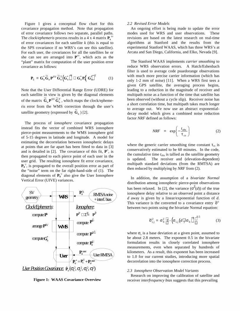
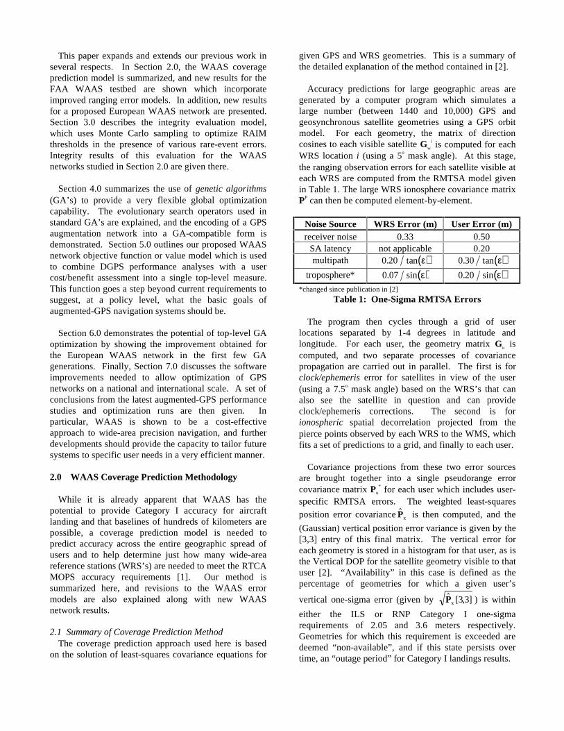
Figure 1 gives a conceptual flow chart for thiscovariance propagation method. Note that propagationof error covariance follows two separate, parallel paths.The clock/ephemeris process results in a 4 x 4 matrix Pk

SV

of error covariances for each satellite k (this is equal tothe SPS covariance if no WRS’s can see this satellite).For each user, the covariances for all the satellites he orshe can see are arranged into PSV, which acts as the“plant” matrix for computation of the user position errorcovariance as follows:

( ) ( )P G G P G G G P G$* * * * *~ ~

x u uSV

uT

u

T

u u

T= + ν (1)

Note that the User Differential Range Error (UDRE) foreach satellite in view is given by the diagonal elements

of the matrix ~ ~G P Gu

SVuT , which maps the clock/epheme-

ris error from the WMS correction through the user’s

satellite geometry (expressed by ~Gu ) [2].

The process of ionosphere covariance propagationinstead fits the vector of combined WRS ionospherepierce-point measurements to the WMS ionosphere gridof 5-15 degrees in latitude and longitude. A model forestimating the decorrelation between ionospheric delaysat points that are far apart has been fitted to data in [3]and is detailed in [2]. The covariance of this fit, PG, isthen propagated to each pierce point of each user in theuser grid. The resulting ionosphere fit error covariance,Pεε

U, is propagated to the overall position error as part ofthe “noise” term on the far right-hand-side of (1). Thediagonal elements of Pεε

U also give the User IonosphereVertical Error (UIVE) variances.

WRS RMTSA noise + interf. bias

compute Pk

Pνk

WMSarrange PSV

Clock/Ephemeris: Ionosphere:

User User RMTSAPν

user

(σx2, σy

2, σz2, σt

2)User Position Covariance:

SV geometry

Pν* = + Pν

user

$Px

P PP P P+ =Σ $

PεU

compute P$G

compute PUG$

computeGu*

PεUcompute

Figure 1: WAAS Covariance Overview

2.2 Revised Error ModelsAn ongoing effort is being made to update the error

modes used for WRS and user observations. Theserevisions are based on the latest research on real-timealgorithms at Stanford and the results from theexperimental Stanford WAAS, which has three WRS’s atArcata and San Diego, California, and Elko, Nevada [9].

The Stanford WAAS implements carrier smoothing toreduce WRS observation errors. A Hatch/Eshenbachfilter is used to average code psuedorange observationswith much more precise carrier information (which hasonly 1-2 mm of noise) [11]. When a WRS first sees agiven GPS satellite, the averaging process begins,leading to a reduction in the magnitude of receiver andmultipath noise as a function of the time that satellite hasbeen observed (without a cycle slip). Receiver noise hasa short correlation time, but multipath takes much longerto average out. We now use an abstract exponential-decay model which gives a combined noise reductionfactor NRF defined as follows:

NRFtobs

cs

= −FHG

IKJexp

τ(2)

where the generic carrier smoothing time constant τcs isconservatively estimated to be 60 minutes. In the code,the cumulative time tobs is tallied as the satellite geometryis updated. The receiver and (elevation-dependent)multipath standard deviations (from the RMTSA) arethen reduced by multiplying by NRF from (2).

In addition, the assumption of a bivariate Normaldistribution among ionospheric pierce-point observations

has been relaxed. In [2], the variance (σ2(d)) of the trueionosphere delay relative to an observed point a distanced away is given by a linear/exponential function of d.This variance is the converted to a covariance entry σ2

between two points using the bivariate Normal equation:

( )( )σ σ σ σi, j2

b i, j b1 -=

2 2 0 5

d.

(3)

where σb is a base deviation at a given point, assumed tobe about 2.8 meters. The exponent 0.5 in the bivariateformulation results in closely correlated ionospheremeasurements, even when separated by hundreds ofkilometers. As a result, this exponent has been increasedto 1.0 for our current studies, introducing more spatialdecorrelation into the ionosphere correction process.

2.3 Ionosphere Observation Model VariantsResearch on improving the calibration of satellite and

receiver interfrequency bias suggests that this prevailing

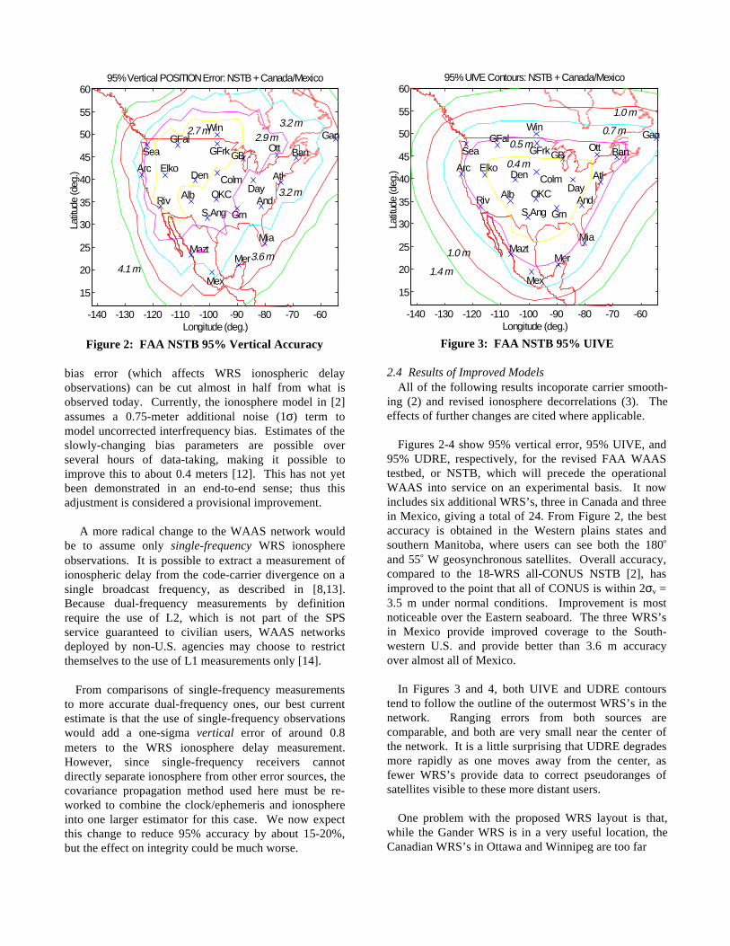
Figure 2: FAA NSTB 95% Vertical Accuracy

bias error (which affects WRS ionospheric delayobservations) can be cut almost in half from what isobserved today. Currently, the ionosphere model in [2]assumes a 0.75-meter additional noise (1σ) term tomodel uncorrected interfrequency bias. Estimates of theslowly-changing bias parameters are possible overseveral hours of data-taking, making it possible toimprove this to about 0.4 meters [12]. This has not yetbeen demonstrated in an end-to-end sense; thus thisadjustment is considered a provisional improvement.

A more radical change to the WAAS network wouldbe to assume only single-frequency WRS ionosphereobservations. It is possible to extract a measurement ofionospheric delay from the code-carrier divergence on asingle broadcast frequency, as described in [8,13].Because dual-frequency measurements by definitionrequire the use of L2, which is not part of the SPSservice guaranteed to civilian users, WAAS networksdeployed by non-U.S. agencies may choose to restrictthemselves to the use of L1 measurements only [14].

From comparisons of single-frequency measurementsto more accurate dual-frequency ones, our best currentestimate is that the use of single-frequency observationswould add a one-sigma vertical error of around 0.8meters to the WRS ionosphere delay measurement.However, since single-frequency receivers cannotdirectly separate ionosphere from other error sources, thecovariance propagation method used here must be re-worked to combine the clock/ephemeris and ionosphereinto one larger estimator for this case. We now expectthis change to reduce 95% accuracy by about 15-20%,but the effect on integrity could be much worse.

Figure 3: FAA NSTB 95% UIVE

2.4 Results of Improved ModelsAll of the following results incoporate carrier smooth-

ing (2) and revised ionosphere decorrelations (3). Theeffects of further changes are cited where applicable.

Figures 2-4 show 95% vertical error, 95% UIVE, and95% UDRE, respectively, for the revised FAA WAAStestbed, or NSTB, which will precede the operationalWAAS into service on an experimental basis. It nowincludes six additional WRS’s, three in Canada and threein Mexico, giving a total of 24. From Figure 2, the bestaccuracy is obtained in the Western plains states andsouthern Manitoba, where users can see both the 180o

and 55o W geosynchronous satellites. Overall accuracy,compared to the 18-WRS all-CONUS NSTB [2], hasimproved to the point that all of CONUS is within 2σv =3.5 m under normal conditions. Improvement is mostnoticeable over the Eastern seaboard. The three WRS’sin Mexico provide improved coverage to the South-western U.S. and provide better than 3.6 m accuracyover almost all of Mexico.

In Figures 3 and 4, both UIVE and UDRE contourstend to follow the outline of the outermost WRS’s in thenetwork. Ranging errors from both sources arecomparable, and both are very small near the center ofthe network. It is a little surprising that UDRE degradesmore rapidly as one moves away from the center, asfewer WRS’s provide data to correct pseudoranges ofsatellites visible to these more distant users.

One problem with the proposed WRS layout is that,while the Gander WRS is in a very useful location, theCanadian WRS’s in Ottawa and Winnipeg are too far

-140 -130 -120 -110 -100 -90 -80 -70 -60

15

20

25

30

35

40

45

50

55

60

Sea

Arc Elko

Riv

GFal

AtlDen

Alb

GFrk

ColmOKC

S.Ang

GB

Day

Grn

Ban

And

Mia

Ott

WinGan

Mex

MaztMer

Longitude (deg.)

Latit

ude

(deg

.)

2.7 m2.9 m

3.2 m

3.2 m

3.6 m4.1 m

95% Vertical POSITION Error: NSTB + Canada/Mexico

-140 -130 -120 -110 -100 -90 -80 -70 -60

15

20

25

30

35

40

45

50

55

60

Sea

Arc Elko

Riv

GFal

AtlDen

Alb

GFrk

ColmOKC

S.Ang

GB

Day

Grn

Ban

And

Mia

Ott

WinGan

Mex

MaztMer

Longitude (deg.)

Latit

ude

(deg

.)

0.4 m

0.5 m0.7 m

1.0 m

1.0 m

1.4 m

95% UIVE Contours: NSTB + Canada/Mexico

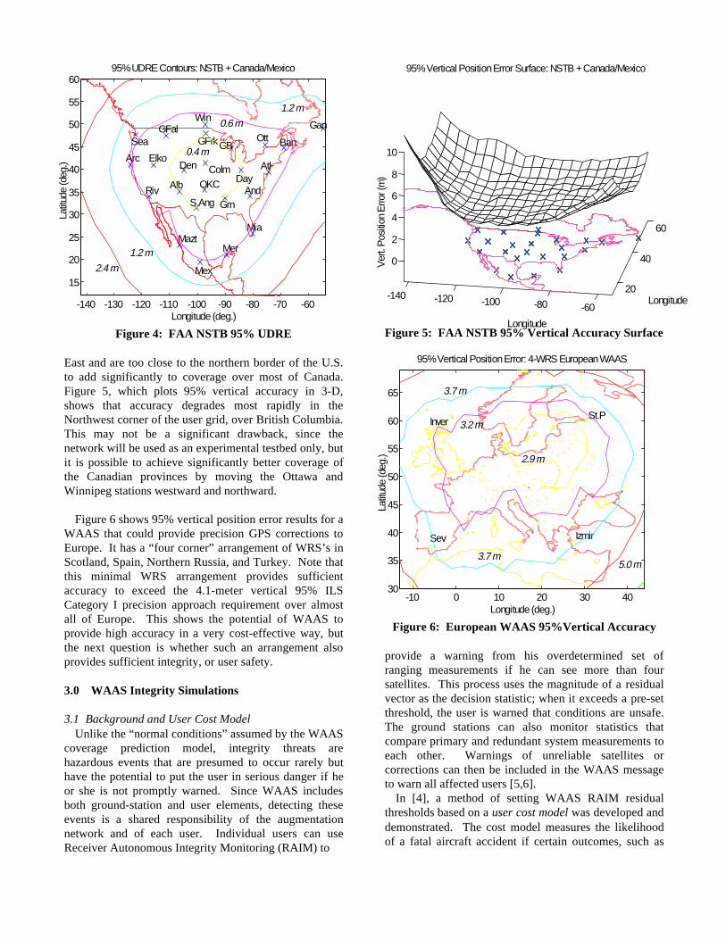
Figure 4: FAA NSTB 95% UDRE

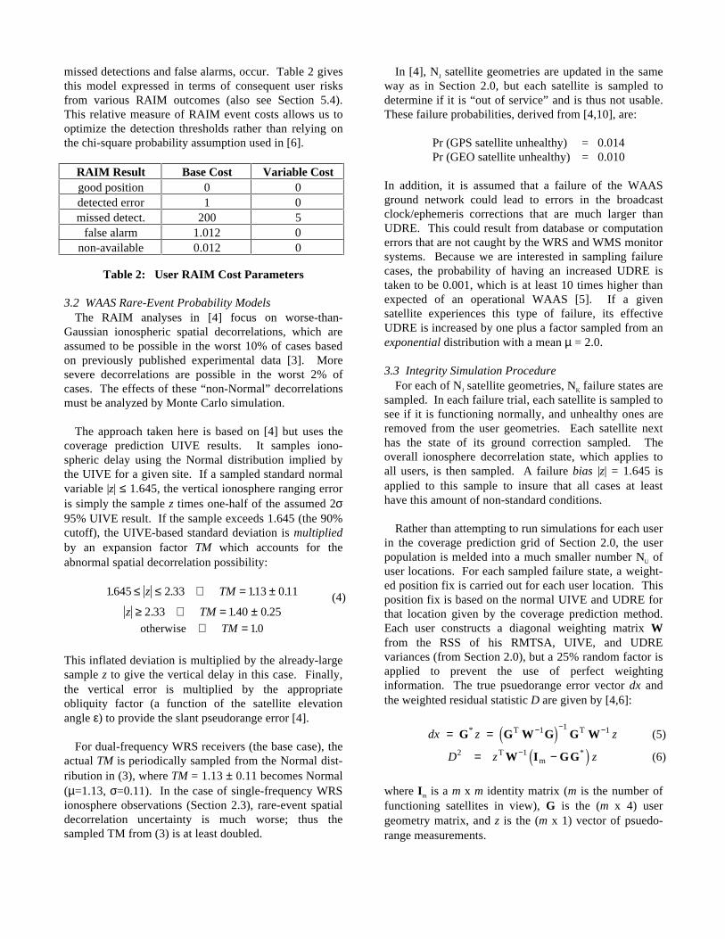
East and are too close to the northern border of the U.S.to add significantly to coverage over most of Canada.Figure 5, which plots 95% vertical accuracy in 3-D,shows that accuracy degrades most rapidly in theNorthwest corner of the user grid, over British Columbia.This may not be a significant drawback, since thenetwork will be used as an experimental testbed only, butit is possible to achieve significantly better coverage ofthe Canadian provinces by moving the Ottawa andWinnipeg stations westward and northward.

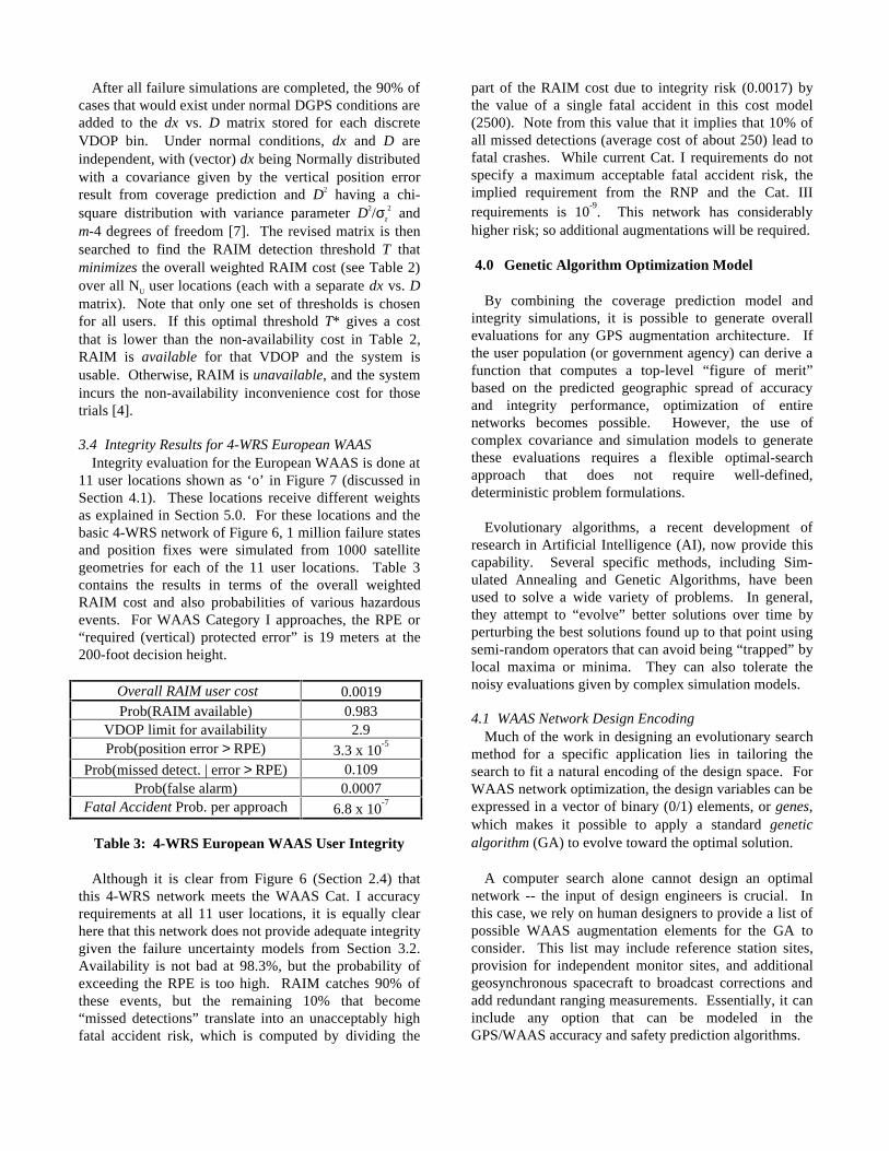
Figure 6 shows 95% vertical position error results for aWAAS that could provide precision GPS corrections toEurope. It has a “four corner” arrangement of WRS’s inScotland, Spain, Northern Russia, and Turkey. Note thatthis minimal WRS arrangement provides sufficientaccuracy to exceed the 4.1-meter vertical 95% ILSCategory I precision approach requirement over almostall of Europe. This shows the potential of WAAS toprovide high accuracy in a very cost-effective way, butthe next question is whether such an arrangement alsoprovides sufficient integrity, or user safety.

3.0 WAAS Integrity Simulations

3.1 Background and User Cost ModelUnlike the “normal conditions” assumed by the WAAS

coverage prediction model, integrity threats arehazardous events that are presumed to occur rarely buthave the potential to put the user in serious danger if heor she is not promptly warned. Since WAAS includesboth ground-station and user elements, detecting theseevents is a shared responsibility of the augmentationnetwork and of each user. Individual users can useReceiver Autonomous Integrity Monitoring (RAIM) to

Figure 5: FAA NSTB 95% Vertical Accuracy Surface

Figure 6: European WAAS 95%Vertical Accuracy

provide a warning from his overdetermined set ofranging measurements if he can see more than foursatellites. This process uses the magnitude of a residualvector as the decision statistic; when it exceeds a pre-setthreshold, the user is warned that conditions are unsafe.The ground stations can also monitor statistics thatcompare primary and redundant system measurements toeach other. Warnings of unreliable satellites orcorrections can then be included in the WAAS messageto warn all affected users [5,6].

In [4], a method of setting WAAS RAIM residualthresholds based on a user cost model was developed anddemonstrated. The cost model measures the likelihoodof a fatal aircraft accident if certain outcomes, such as

-140 -130 -120 -110 -100 -90 -80 -70 -60

15

20

25

30

35

40

45

50

55

60

Sea

Arc Elko

Riv

GFal

AtlDen

Alb

GFrk

ColmOKC

S.Ang

GB

Day

Grn

Ban

And

Mia

Ott

WinGan

Mex

MaztMer

Longitude (deg.)

Latit

ude

(deg

.)

0.4 m

0.6 m

1.2 m

1.2 m

2.4 m

95% UDRE Contours: NSTB + Canada/Mexico

-140 -120 -100 -80 -60

20

40

60

0

2

4

6

8

10

Longitude

Longitude

Ver

t. P

ositi

on E

rror (

m)

95% Vertical Position Error Surface: NSTB + Canada/Mexico

-10 0 10 20 30 4030

35

40

45

50

55

60

65

Inver

Sev

St.P

Izmir

Longitude (deg.)

Latit

ude

(deg

.) 2.9 m

3.2 m

3.7 m

3.7 m

5.0 m

95% Vertical Position Error: 4-WRS European WAAS

missed detections and false alarms, occur. Table 2 givesthis model expressed in terms of consequent user risksfrom various RAIM outcomes (also see Section 5.4).This relative measure of RAIM event costs allows us tooptimize the detection thresholds rather than relying onthe chi-square probability assumption used in [6].

RAIM Result Base Cost Variable Costgood position 0 0detected error 1 0missed detect. 200 5

false alarm 1.012 0non-available 0.012 0

Table 2: User RAIM Cost Parameters

3.2 WAAS Rare-Event Probability ModelsThe RAIM analyses in [4] focus on worse-than-

Gaussian ionospheric spatial decorrelations, which areassumed to be possible in the worst 10% of cases basedon previously published experimental data [3]. Moresevere decorrelations are possible in the worst 2% ofcases. The effects of these “non-Normal” decorrelationsmust be analyzed by Monte Carlo simulation.

The approach taken here is based on [4] but uses thecoverage prediction UIVE results. It samples iono-spheric delay using the Normal distribution implied bythe UIVE for a given site. If a sampled standard normalvariable |z| ≤ 1.645, the vertical ionosphere ranging erroris simply the sample z times one-half of the assumed 2σ95% UIVE result. If the sample exceeds 1.645 (the 90%cutoff), the UIVE-based standard deviation is multipliedby an expansion factor TM which accounts for theabnormal spatial decorrelation possibility:

1645 2 33 113 0 11. . . .≤ ≤ ⇒ = ±z TM (4)z TM≥ ⇒ = ±2 33 1 0 25. .40 .

otherwise ⇒ =TM 10.

This inflated deviation is multiplied by the already-largesample z to give the vertical delay in this case. Finally,the vertical error is multiplied by the appropriateobliquity factor (a function of the satellite elevationangle ε) to provide the slant pseudorange error [4].

For dual-frequency WRS receivers (the base case), theactual TM is periodically sampled from the Normal dist-ribution in (3), where TM = 1.13 ± 0.11 becomes Normal(µ=1.13, σ=0.11). In the case of single-frequency WRSionosphere observations (Section 2.3), rare-event spatialdecorrelation uncertainty is much worse; thus thesampled TM from (3) is at least doubled.

In [4], NJ satellite geometries are updated in the sameway as in Section 2.0, but each satellite is sampled todetermine if it is “out of service” and is thus not usable.These failure probabilities, derived from [4,10], are:

Pr (GPS satellite unhealthy) = 0.014Pr (GEO satellite unhealthy) = 0.010

In addition, it is assumed that a failure of the WAASground network could lead to errors in the broadcastclock/ephemeris corrections that are much larger thanUDRE. This could result from database or computationerrors that are not caught by the WRS and WMS monitorsystems. Because we are interested in sampling failurecases, the probability of having an increased UDRE istaken to be 0.001, which is at least 10 times higher thanexpected of an operational WAAS [5]. If a givensatellite experiences this type of failure, its effectiveUDRE is increased by one plus a factor sampled from anexponential distribution with a mean µ = 2.0.

3.3 Integrity Simulation ProcedureFor each of NJ satellite geometries, NK failure states are

sampled. In each failure trial, each satellite is sampled tosee if it is functioning normally, and unhealthy ones areremoved from the user geometries. Each satellite nexthas the state of its ground correction sampled. Theoverall ionosphere decorrelation state, which applies toall users, is then sampled. A failure bias |z| = 1.645 isapplied to this sample to insure that all cases at leasthave this amount of non-standard conditions.

Rather than attempting to run simulations for each userin the coverage prediction grid of Section 2.0, the userpopulation is melded into a much smaller number NU ofuser locations. For each sampled failure state, a weight-ed position fix is carried out for each user location. Thisposition fix is based on the normal UIVE and UDRE forthat location given by the coverage prediction method.Each user constructs a diagonal weighting matrix Wfrom the RSS of his RMTSA, UIVE, and UDREvariances (from Section 2.0), but a 25% random factor isapplied to prevent the use of perfect weightinginformation. The true psuedorange error vector dx andthe weighted residual statistic D are given by [4,6]:

dx z z= = − − −G G W G G W* T T1 1 1d i (5)

D z z2 1= −−TmW I GG*d i (6)

where Im is a m x m identity matrix (m is the number offunctioning satellites in view), G is the (m x 4) usergeometry matrix, and z is the (m x 1) vector of psuedo-range measurements.

After all failure simulations are completed, the 90% ofcases that would exist under normal DGPS conditions areadded to the dx vs. D matrix stored for each discreteVDOP bin. Under normal conditions, dx and D areindependent, with (vector) dx being Normally distributedwith a covariance given by the vertical position errorresult from coverage prediction and D2 having a chi-square distribution with variance parameter D2/σz

2 andm-4 degrees of freedom [7]. The revised matrix is thensearched to find the RAIM detection threshold T thatminimizes the overall weighted RAIM cost (see Table 2)over all NU user locations (each with a separate dx vs. Dmatrix). Note that only one set of thresholds is chosenfor all users. If this optimal threshold T* gives a costthat is lower than the non-availability cost in Table 2,RAIM is available for that VDOP and the system isusable. Otherwise, RAIM is unavailable, and the systemincurs the non-availability inconvenience cost for thosetrials [4].

3.4 Integrity Results for 4-WRS European WAASIntegrity evaluation for the European WAAS is done at

11 user locations shown as ‘o’ in Figure 7 (discussed inSection 4.1). These locations receive different weightsas explained in Section 5.0. For these locations and thebasic 4-WRS network of Figure 6, 1 million failure statesand position fixes were simulated from 1000 satellitegeometries for each of the 11 user locations. Table 3contains the results in terms of the overall weightedRAIM cost and also probabilities of various hazardousevents. For WAAS Category I approaches, the RPE or“required (vertical) protected error” is 19 meters at the200-foot decision height.

Overall RAIM user cost 0.0019Prob(RAIM available) 0.983

VDOP limit for availability 2.9Prob(position error > RPE) 3.3 x 10

-5

Prob(missed detect. | error > RPE) 0.109Prob(false alarm) 0.0007

Fatal Accident Prob. per approach 6.8 x 10-7

Table 3: 4-WRS European WAAS User Integrity

Although it is clear from Figure 6 (Section 2.4) thatthis 4-WRS network meets the WAAS Cat. I accuracyrequirements at all 11 user locations, it is equally clearhere that this network does not provide adequate integritygiven the failure uncertainty models from Section 3.2.Availability is not bad at 98.3%, but the probability ofexceeding the RPE is too high. RAIM catches 90% ofthese events, but the remaining 10% that become“missed detections” translate into an unacceptably highfatal accident risk, which is computed by dividing the

part of the RAIM cost due to integrity risk (0.0017) bythe value of a single fatal accident in this cost model(2500). Note from this value that it implies that 10% ofall missed detections (average cost of about 250) lead tofatal crashes. While current Cat. I requirements do notspecify a maximum acceptable fatal accident risk, theimplied requirement from the RNP and the Cat. IIIrequirements is 10

-9. This network has considerably

higher risk; so additional augmentations will be required.

4.0 Genetic Algorithm Optimization Model

By combining the coverage prediction model andintegrity simulations, it is possible to generate overallevaluations for any GPS augmentation architecture. Ifthe user population (or government agency) can derive afunction that computes a top-level “figure of merit”based on the predicted geographic spread of accuracyand integrity performance, optimization of entirenetworks becomes possible. However, the use ofcomplex covariance and simulation models to generatethese evaluations requires a flexible optimal-searchapproach that does not require well-defined,deterministic problem formulations.

Evolutionary algorithms, a recent development ofresearch in Artificial Intelligence (AI), now provide thiscapability. Several specific methods, including Sim-ulated Annealing and Genetic Algorithms, have beenused to solve a wide variety of problems. In general,they attempt to “evolve” better solutions over time byperturbing the best solutions found up to that point usingsemi-random operators that can avoid being “trapped” bylocal maxima or minima. They can also tolerate thenoisy evaluations given by complex simulation models.

4.1 WAAS Network Design EncodingMuch of the work in designing an evolutionary search

method for a specific application lies in tailoring thesearch to fit a natural encoding of the design space. ForWAAS network optimization, the design variables can beexpressed in a vector of binary (0/1) elements, or genes,which makes it possible to apply a standard geneticalgorithm (GA) to evolve toward the optimal solution.

A computer search alone cannot design an optimalnetwork -- the input of design engineers is crucial. Inthis case, we rely on human designers to provide a list ofpossible WAAS augmentation elements for the GA toconsider. This list may include reference station sites,provision for independent monitor sites, and additionalgeosynchronous spacecraft to broadcast corrections andadd redundant ranging measurements. Essentially, it caninclude any option that can be modeled in theGPS/WAAS accuracy and safety prediction algorithms.

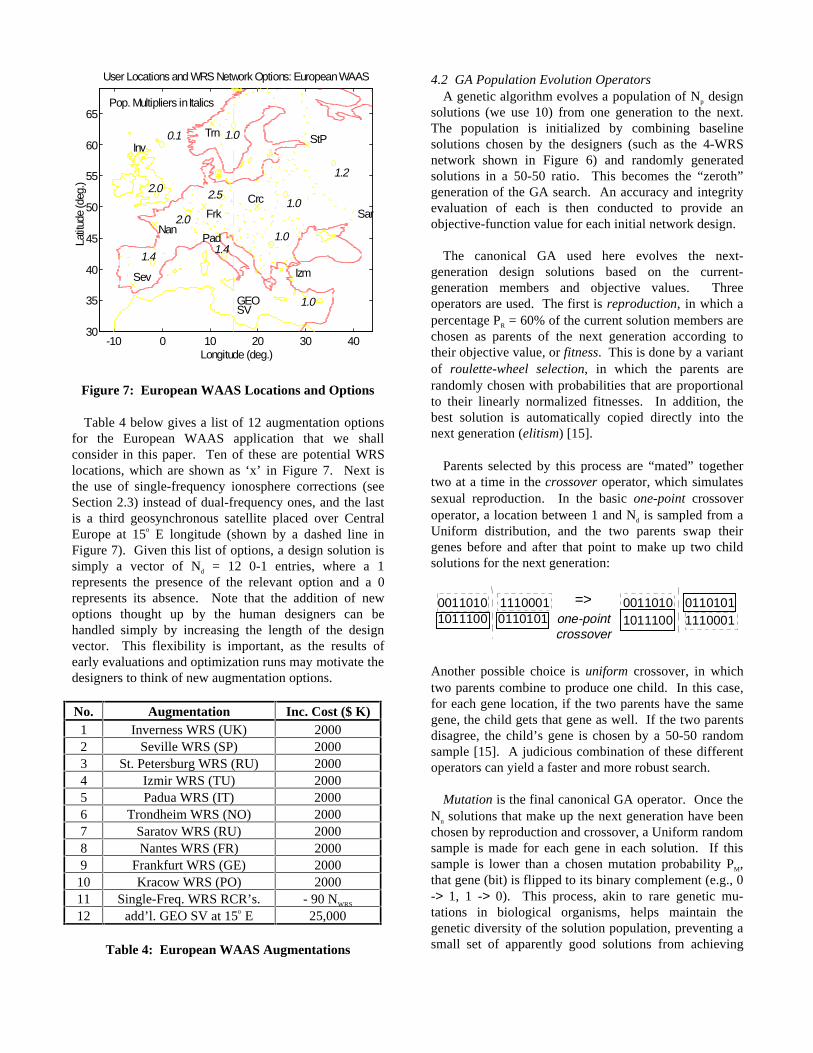
Figure 7: European WAAS Locations and Options

Table 4 below gives a list of 12 augmentation optionsfor the European WAAS application that we shallconsider in this paper. Ten of these are potential WRSlocations, which are shown as ‘x’ in Figure 7. Next isthe use of single-frequency ionosphere corrections (seeSection 2.3) instead of dual-frequency ones, and the lastis a third geosynchronous satellite placed over CentralEurope at 15o E longitude (shown by a dashed line inFigure 7). Given this list of options, a design solution issimply a vector of Nd = 12 0-1 entries, where a 1represents the presence of the relevant option and a 0represents its absence. Note that the addition of newoptions thought up by the human designers can behandled simply by increasing the length of the designvector. This flexibility is important, as the results ofearly evaluations and optimization runs may motivate thedesigners to think of new augmentation options.

No. Augmentation Inc. Cost ($ K)1 Inverness WRS (UK) 20002 Seville WRS (SP) 20003 St. Petersburg WRS (RU) 20004 Izmir WRS (TU) 20005 Padua WRS (IT) 20006 Trondheim WRS (NO) 20007 Saratov WRS (RU) 20008 Nantes WRS (FR) 20009 Frankfurt WRS (GE) 200010 Kracow WRS (PO) 200011 Single-Freq. WRS RCR’s. - 90 NWRS

12 add’l. GEO SV at 15o E 25,000

Table 4: European WAAS Augmentations

4.2 GA Population Evolution OperatorsA genetic algorithm evolves a population of Np design

solutions (we use 10) from one generation to the next.The population is initialized by combining baselinesolutions chosen by the designers (such as the 4-WRSnetwork shown in Figure 6) and randomly generatedsolutions in a 50-50 ratio. This becomes the “zeroth”generation of the GA search. An accuracy and integrityevaluation of each is then conducted to provide anobjective-function value for each initial network design.

The canonical GA used here evolves the next-generation design solutions based on the current-generation members and objective values. Threeoperators are used. The first is reproduction, in which apercentage PR = 60% of the current solution members arechosen as parents of the next generation according totheir objective value, or fitness. This is done by a variantof roulette-wheel selection, in which the parents arerandomly chosen with probabilities that are proportionalto their linearly normalized fitnesses. In addition, thebest solution is automatically copied directly into thenext generation (elitism) [15].

Parents selected by this process are “mated” togethertwo at a time in the crossover operator, which simulatessexual reproduction. In the basic one-point crossoveroperator, a location between 1 and Nd is sampled from aUniform distribution, and the two parents swap theirgenes before and after that point to make up two childsolutions for the next generation:

=>one-pointcrossover

0011010 11100011011100 0110101

0011010 01101011011100 1110001

Another possible choice is uniform crossover, in whichtwo parents combine to produce one child. In this case,for each gene location, if the two parents have the samegene, the child gets that gene as well. If the two parentsdisagree, the child’s gene is chosen by a 50-50 randomsample [15]. A judicious combination of these differentoperators can yield a faster and more robust search.

Mutation is the final canonical GA operator. Once theNn solutions that make up the next generation have beenchosen by reproduction and crossover, a Uniform randomsample is made for each gene in each solution. If thissample is lower than a chosen mutation probability PM,that gene (bit) is flipped to its binary complement (e.g., 0-> 1, 1 -> 0). This process, akin to rare genetic mu-tations in biological organisms, helps maintain thegenetic diversity of the solution population, preventing asmall set of apparently good solutions from achieving

-10 0 10 20 30 4030

35

40

45

50

55

60

65

Inv

Sev

StP

Izm

Trn

FrkNan

CrcSar

Pad

0.1

2.0

1.4

2.0

1.0

2.5

1.4

1.2

1.0

1.0

1.0GEOSV

Pop. Multipliers in Italics

Longitude (deg.)

Latit

ude

(deg

.)User Locations and WRS Network Options: European WAAS

premature dominance (i.e., a local optimum). Normally,PM is chosen to be ≤ 0.01 (we have chosen 0.01), buthigher mutation rates (inducing more diversity) havebeen successful for other problems [15].

001100111001 => 001101111001one-bit mutation

4.3 GA Optimization ProcedureFigure 8 gives a flow chart of the procedure by which

the GA “breeds” new generations of solutions and eval-uates their fitnesses. Generation 0 is initialized as men-tioned in Section 4.1, then a loop of generations begins.Given a generation n, the fitnesses of each of its Np

solution members are evaluated using both coverage(Section 2.0) and integrity (Section 3.0) analyses fed intothe cost model of Section 5.0. Reproduction, crossover,and mutation are then applied to generate the newgeneration n+1. The GA evolution can be stopped whenthe population (or the value of its best solution) stopsimproving, or it can be ended after a set number ofgenerations. Each re-evaluation of a given network isadded to those conducted previously; thus statisticalsignificance increases with each new evaluation. Once agiven network evaluation converges to within anuncertainty tolerance, no further accuracy/integrityevaluations are needed. Therefore, later GA generationswill run faster on the computer than earlier ones.

Figure 8: GA Optimization Procedure

5.0 WAAS Network Objective Function

Each of the possible solutions generated by GA evo-lution needs a fitness evaluation, or a measure of itsrelative “goodness”. Because GA optimization is veryflexible, there are no mathematical constraints on theform of this system objective function. We can thus

construct a “value model” that attempts to express thesystem’s top-level utility for the total user population.This is a key driver of the optimization process, as theGA evolution will tend to exploit any inconsistency or“hole” in the fitness model. For this reason, theelements of the objective function should be carefullyconsidered, and the results of early GA runs maymotivate changes in the value model.

The value model developed here is a provisionalattempt to weigh user benefits and system costs in aswide a framework as possible, knowing that substantialrevisions may be necessary as more designer and userinput is received. The overall objective function F(n) tobe maximized is given by:

F n PM B f f LCostuu

u u unWAAS air acc intega f = − −

=∑

1

11

(7)

where facc

u and finteg

u represent evaluations of coverage andintegrity performance respectively for user location u,Bair

u is the Cat. I user benefit for a given user location,PMu is a “population multiplier” which measures the sizeof the user population near that location, and LCostn isthe acquisition cost of a given WAAS network solutionn, which includes the procurement cost and four years ofOEM (operations and maintenance).

5.1 Population MultiplierThe basic definition for the population multiplier is:

PMp p p p

ii c i c= >R

STwhere

otherwise1(8)

where pi is the user population (which could be totalpopulation, number of air passengers, etc.) and pc is a“critical value” which insures that all areas covered byWAAS get a minimum base priority. Locations whichexceed this critical value do get a higher priority, but itdoes not scale linearly. The values of PM for the 11 userlocations selected for the European WAAS is shown inFigure 7. Note that the location over the North Sea isvalued at 10% of the overland site values since precisionapproaches cannot be done there. The maximum valueof 2.5 given to the Leipzig, Ger. user location implies acritical value for overall population of about 8 million.

5.2 Network Acquisition CostsThe system acquisition cost for all WAAS networks

assumes a well-equipped triply-redundant hardwaresetup at all ground stations. It includes a WMSprocurement cost estimated at $6 million and four yearsof OEM at $2 million/year, giving a WMS acquisitioncost of around $14 million. The incremental WRS cost

WAAS baselinedesign pop.

iterate

WAAS Coverage Prediction Eval.

simulation-based integrity evaluation

optimalthresholds

NO

YES

rare-eventionosphere

model

WAASfailuremodel

converged?

optimal design :review and compare

Generation 0

clock/ephemeris

ionospheregrid

GA Repro-duction

valuemodel

GA Crossover

GA Mutation

next-gen.population

estimated to be $1.1 million, includes a $0.5 millionprocurement cost and $150 thousand per-year OEM cost.The cost savings obtained by using single-frequencyreceivers in the WRS’s is estimated at 75% of the cost ofa dual-frequency receiver set mutiplied by the number ofWRS’s in a given solution. For all ground augmenta-tions, an 80% administrative and indirect cost factor isadded, giving conservative final life cycle costs of $25million for a WMS and $2 million for each WRS (asshown in Table 4). This is based on the high overall costestimates for the FAA WAAS given in [16]. Finally, thecost of providing an additional geosynchronous satelliteis assumed to be $25 million, the estimated cost of aninexpensive satellite designed for just this purpose. Asin the Inmarsat case, leasing a GEO transponder may bean option, but the high value of the 15o E locationsuggests even a lease cost will be much higher than the$2 million/year paid by the FAA. The sensitivity of theoptimal result to this cost should be examined further.

5.3 User Benefit EstimatesThe calculation of benefits provided by Category I to

precision approach users requires making significantassumptions. According to [17], WAAS is expected toincrease the number of Category I approaches in the U.S.from 765 (in 1994) to over 5,000. It also suggests anoverall user benefit for WAAS Cat. I to be $992 million,or about $200,000 per approach. In Europe, we estimatethat this life-cycle per-approach benefit will be doubleddue to the poorer weather there. In [18], Europe is es-timated to have 326 Cat. I ILS facilities (1994), and weconservatively assume that WAAS will allow this togrow to 1200, giving a total user benefit of $480 million.

An estimate of the per-approach benefit of having Cat.I available is estimated by [18] as saving 2 minutes.Converted to aircraft per-hour fuel and direct operatingcosts of a weighted mix of passenger aircraft (about$4800), the benefit (conservatively) becomes an averageof $160 per approach. Given 1200 Cat. I approacheseach providing benefits of $400,000 on average over afour-year life cycle, approximately 3 million Cat. Iapproaches in Europe are expected in during this time.

A second user benefit to WAAS is removing the needto support and maintain the 326 current ILS facilitiesthat now provide Cat. I capability. This cost is estimatedby [18] to be $400,000 per ILS facility (per life cycle),which, multiplied by 326, gives an added benefit toWAAS of $130 million. While it can be argued [14] thatthe current ILS network has been recently upgraded andrepresents a “sunk cost,” the continual maintenance of itwould no longer be necessary after WAAS becomesoperational. Under this model, the total life-cyclebenefit of WAAS Cat. I is $610 million.

5.4 Accuracy and Integrity EvaluationThe WAAS accuracy evaluation facc

u is simply a per-centage of the benefit for each user location, which isbroken down from the $610 million total based on thepopulation multiplier for that site. Perfect navigationgets 100% credit, a 2σ vertical error of 2.1 m gets 99%,4.1 m (the ILS requirement) gets 90%, and 7.6 m (theWAAS RNP requirement) gets only 20% (since it is atthe outermost limit of acceptability). A cubic polyno-mial fit gives, for a resulting 2σ vertical accuracy a (m):

f a a auacc = − + −1 0 005 0 0052 0 00242 3. . . (9)

where facc

u is in decimal terms (i.e. from 0 to 1).

Converting the RAIM user cost of Section 3.1 to thisvalue framework requires two further assumptions. InProbabilistic Risk Assessment (PRA), it is consideredvalid to assign cost values to fatalities if the underlyingrisk is sufficiently small (below 10

-4) [19], which it is for

GPS integrity. Assuming an average (based on thebreakdown of aircraft sizes for Cat. I approaches) of 100fatalities per fatal incident and a conservative “value perlife” of $10 million, each fatal accident incurs a loss ofabout $1 billion. Since 3 million approaches are fore-seen over the 4-year life cycle, and a fatal accidentimplies a cost of 2500 in the RAIM cost model, we canconvert from RAIM cost (Rc) to overall value (finteg

tot):

f R Rtotinteg c c=

× ×= ×

$1.

10 3 10

25001 2 10

9 612d id i

(10)

Note that this calculation is also broken down by userlocation and population multiplier within the RAIM usercost optimization (Section 3.3). Also note that the non-availability cost per approach (0.012) from Table 2,which is included in the integrity evaluation, implies anuisance cost equivalent to an average of an hour ofadded aircraft cost, including all consequent delays.

5.5 Value of 4-WRS Baseline European WAASThe accuracy of the baseline 4-WRS European WAAS

network (shown in Figure 6) translates into a accuracymultiplier (weighted by PM) of 0.958, giving an overalluser benefit of $584 million. However, the RAIM usercost of 0.0019 from Table 3 translates (using (10)) intoan integrity cost of $1.73 billion, or 3 times the userbenefit. Clearly, this network is insufficient. Note thatthe acquisition cost of $33 million is dwarfed by thebenefits and costs that result, indicating that additionalaugmentations would be very cheap relative to thepossible performance improvement. Also, the fact that a4-WRS WAAS network cannot provide sufficientintegrity suggests that proposed augmented-GPS systems

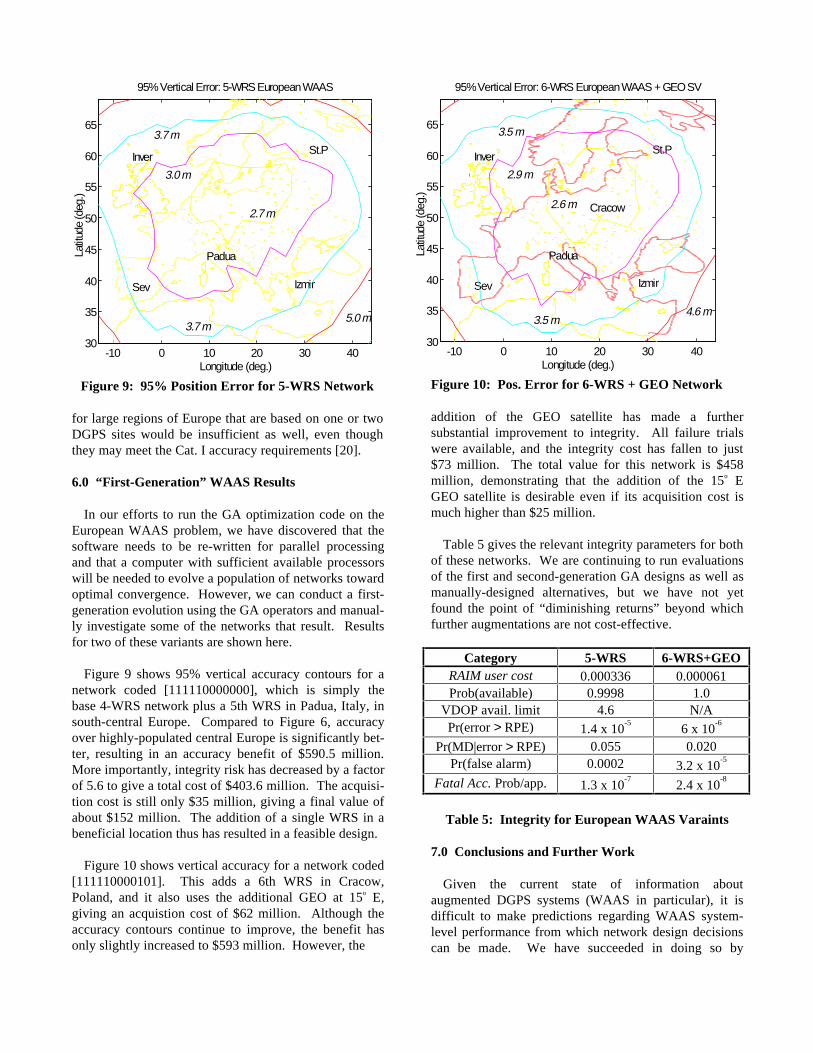
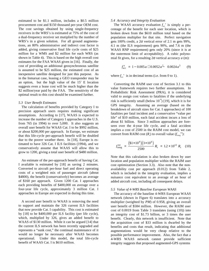
Figure 9: 95% Position Error for 5-WRS Network

for large regions of Europe that are based on one or twoDGPS sites would be insufficient as well, even thoughthey may meet the Cat. I accuracy requirements [20].

6.0 “First-Generation” WAAS Results

In our efforts to run the GA optimization code on theEuropean WAAS problem, we have discovered that thesoftware needs to be re-written for parallel processingand that a computer with sufficient available processorswill be needed to evolve a population of networks towardoptimal convergence. However, we can conduct a first-generation evolution using the GA operators and manual-ly investigate some of the networks that result. Resultsfor two of these variants are shown here.

Figure 9 shows 95% vertical accuracy contours for anetwork coded [111110000000], which is simply thebase 4-WRS network plus a 5th WRS in Padua, Italy, insouth-central Europe. Compared to Figure 6, accuracyover highly-populated central Europe is significantly bet-ter, resulting in an accuracy benefit of $590.5 million.More importantly, integrity risk has decreased by a factorof 5.6 to give a total cost of $403.6 million. The acquisi-tion cost is still only $35 million, giving a final value ofabout $152 million. The addition of a single WRS in abeneficial location thus has resulted in a feasible design.

Figure 10 shows vertical accuracy for a network coded[111110000101]. This adds a 6th WRS in Cracow,Poland, and it also uses the additional GEO at 15o E,giving an acquistion cost of $62 million. Although theaccuracy contours continue to improve, the benefit hasonly slightly increased to $593 million. However, the

Figure 10: Pos. Error for 6-WRS + GEO Network

addition of the GEO satellite has made a furthersubstantial improvement to integrity. All failure trialswere available, and the integrity cost has fallen to just$73 million. The total value for this network is $458million, demonstrating that the addition of the 15o EGEO satellite is desirable even if its acquisition cost ismuch higher than $25 million.

Table 5 gives the relevant integrity parameters for bothof these networks. We are continuing to run evaluationsof the first and second-generation GA designs as well asmanually-designed alternatives, but we have not yetfound the point of “diminishing returns” beyond whichfurther augmentations are not cost-effective.

Category 5-WRS 6-WRS+GEORAIM user cost 0.000336 0.000061Prob(available) 0.9998 1.0

VDOP avail. limit 4.6 N/APr(error > RPE) 1.4 x 10

-56 x 10

-6

Pr(MD|error > RPE) 0.055 0.020Pr(false alarm) 0.0002 3.2 x 10

-5

Fatal Acc. Prob/app. 1.3 x 10-7

2.4 x 10-8

Table 5: Integrity for European WAAS Varaints

7.0 Conclusions and Further Work

Given the current state of information aboutaugmented DGPS systems (WAAS in particular), it isdifficult to make predictions regarding WAAS system-level performance from which network design decisionscan be made. We have succeeded in doing so by

-10 0 10 20 30 4030

35

40

45

50

55

60

65

Inver

Sev

St.P

Izmir

Padua

Longitude (deg.)

Latit

ude

(deg

.)

2.7 m

3.0 m

3.7 m

3.7 m

5.0 m

95% Vertical Error: 5-WRS European WAAS

-10 0 10 20 30 4030

35

40

45

50

55

60

65

Inver

Sev

St.P

Izmir

Padua

Cracow

Longitude (deg.)

Latit

ude

(deg

.)

2.6 m

2.9 m

3.5 m

3.5 m4.6 m

95% Vertical Error: 6-WRS European WAAS + GEO SV

developing algorithms that combine covariance pro-pagation to determine position accuracy for large areasof potential users with failure-case simulations thatincorporate the best available current knowledge.Further improvements in these prediction methods arepossible, including fitting more detailed error models tothe rapidly-growing Stanford WAAS database. Bettermodels of ground integrity can also be developed, allow-ing us to add detailed ground integrity monitor optimiza-tion to our current optimal-RAIM algorithm. Finally, thewealth of data to be collected by the FAA’s NSTBstarting in 1997 should dramatically reduce our uncer-tainty about potential failure sources, most notablyincluding ionospheric spatial decorrelation.

The augmented-GPS network optimization results wehave achieved to date are impressive. We have demon-strated the policy-level feasibility and desirability ofusing WAAS to provide Category I precision approachcapability to Europe with the network designs of Section6.0, and we are continuing to search for the best possiblecombination of WRS’s and geosynchronous satellites toaccomplish this. The 6-WRS + GEO SV combinationlooks very promising, as it meets all implied Cat. Irequirements and provides a value benefit of over $450million, depending on the cost of the GEO. We plan toexpand the applicability of our optimization approach byrevising the assumptions of European value model fornetworks in North America and the rest of the world.

As noted before, our ability to make this vision ofaugmented-GPS evolutionary optimization a realityrequires implementing the coverage prediction andintegrity simulation software on a multi-processorcomputer. This is intuitively easy because the evaluationof accuracy or integrity for each user location is a similarprocess that can be done simultaneously for as manylocations as there are available processors. Stanford’sGPS research groups plan to acquire a workstation withat least 16 fast processors by early next year. Thiscomputer will be used for extensive simulations of bothLAAS and WAAS architectures, as Stanford iscontracted by the FAA to evaluate the cost-benefitperformance and certifiability of various competingLAAS systems. This work will utilize and furtherdevelop the GPS evaluation and optimization techniquesreported in this paper.

ACKNOWLEDGEMENTS

The authors would like to thank the following peoplefor their help with this research and the software onwhich it is based: Y.C. Chao, Dave Lawrence, Dr.Changdon Kee, Boris Pervan, Y.J. Tsai, and Dr. ToddWalter. The advice and interest of many other people in

the Stanford GPS research group is appreciated, as isfunding support from NASA, the FAA, and BoeingCommercial Airplane Group.

REFERENCES

[1] P. Enge and A.J. Van Dierendonck, "The Wide AreaAugmentation System", Proc. 8th Int'l. Flight InspectionSymposium, Denver, CO., June 1994.

[2] S. Pullen, P. Enge, B. Parkinson, “A New Methodfor Coverage Analysis for the Wide Area AugmentationSystem (WAAS)”, Proc. of ION 51st Annual Meeting,Colorado Springs, CO., June 5-7, 1995, pp. 501-513.

[3] J.A. Klobuchar, P.H. Doherty, and M.B. El-Arini,"Potential Ionospheric Limitations to Wide-AreaDifferential GPS", Proceedings of ION GPS-93, SaltLake City, UT., Sept. 22-24, 1993, pp. 1245-1254.

[4] S. Pullen, P. Enge, B. Parkinson, “Simulation-BasedEvaluation of WAAS Performance: Risk and IntegrityFactors”, Proceedings of ION GPS-94. Salt Lake City,UT., Sept. 20-23, 1994, pp. 975-983.

[5] R. Loh and J.P. Fernow, "Integrity Concepts for aGPS Wide-Area Augmentation System (WAAS)",Proceedings of ION NTM-94, San Diego, CA., Jan. 24-26, 1994, pp. 127-134.

[6] T. Walter, P. Enge, F. Van Graas, "Integrity for theWide Area Augmentation System", Proceedings ofDSNS-95. Bergen, Norway, April 24-28, 1995, No. 38. [7] S. Pullen and B. Parkinson, "A New Approach toGPS Integrity Monitoring using Prior Probabilities andOptimal Threshold Search", Proceedings of IEEE PLANS'94. Las Vegas, NV., April 11-15, 1994, pp. 739-746.

[8] V. Ashkenazi, C.J. Hill, J. Nagel, “Wide Area Diffe-rential GPS: A Performance Study”, Proc. of ION GPS-92, Albuquerque, NM., Sept. 16-18, 1992, pp. 589-598.

[9] T. Walter, C. Kee, et.al., “Flight Trials of the WideArea Augmentation System (WAAS)”, Proc. of IONGPS-94. Salt Lake City, UT., Sept. 20-23, 1994, pp.1537-1546.

[10] W. Phlong, B. Elrod, "Availability Characteristicsof GPS and Augmentation Alternatives", Navigation,Vol. 40, No. 4, Winter 1993-94, pp. 409-428.

[11] R. Hatch, “The Synergism of GPS Code and CarrierMeasurements”, Proc. 3rd Int’l. Geodetic Symposium on

Satellite Doppler Positioning, Las Cruces, NM., Feb.1982, pp. 1213-1232.

[12] Y.C. Chao, Y.J. Tsai, et.al., “An Algorithm forInter-Frequency Bias Calibration and Application toWAAS Ionosphere Modeling”, Proc. of ION GPS-95,Palm Springs, CA., Sept. 12-15, 1995.

[13] C. Cohen, B. Pervan, B. Parkinson, “Estimation ofAbsolute Ionospheric Delay Exclusively through Single-Frequency GPS Measurements”, Proc. of ION GPS-92,Albuquerque, NM., Sept. 16-18, 1992, pp. 325-330.

[14] W. Lechner, private conversation, Stanford GPSResearch presentation, August 11, 1995.

[15] L. Davis, Ed., Handbook of Genetic Algorithms.New York: Van Nostrand Reinhold, 1991.

[16] A Technical Report to the Secretary of Transpor-tation on a National Approach to Augmented GPSServices. U.S. Department of Commerce, NTIA SpecialPublication 94-30, December 1994.

[17] FAA HDQTRS - APO, “Projected GNSS Cat I/II/IIIPrecision Landing Operations”, Proc. of ICAO Comm./Ops. Meeting. Montreal: Mar. 27-Apr. 7, 1995. Item 1.

[18] ICAO Secretariat, “Economic Evaluations of theMain Options for Precision Approach and LandingSystems”, Proc. of ICAO Comm./Ops. Meeting.Montreal: Mar. 27-Apr. 7, 1995, Item 2-3, WP/23.

[19] J.D. Graham and J.W. Vaupel, "Value of a Life:What Difference Does It Make?”, Risk Analysis, Vol. 1,No. 1, 1981, pp. 89-95.

[20] G. Schanzer, "Satellite Navigation for PrecisionApproach: Technological and Political Benefits andRisks”, Proeedings of ISPA ‘95. Braunschweig, Ger.,Feb. 21-24, 1995, pp. 25-30.