Global Optimization for Scheduling Refinery Crude Oil Operations

Global Optimization for Scheduling Refinery Crude Oil Operations

Ramkumar Karuppiaha, Kevin C. Furmanb and Ignacio E. Grossmanna* a Department of Chemical Engineering, Carnegie Mellon University, Pittsburgh, PA

15213, U.S.A.

b ExxonMobil Research and Engineering, Annandale, NJ 08801, U.S.A.

April 2007

ABSTRACT

In this work we present an Outer-Approximation algorithm to obtain the global

optimum of a nonconvex Mixed Integer Nonlinear Programming (MINLP) model for the

scheduling of crude oil movement at the front-end of a petroleum refinery. The model

relies on a continuous time representation making use of transfer events. The proposed

technique focuses on effectively solving a Mixed Integer Linear Programming (MILP)

relaxation of the nonconvex MINLP to obtain a rigorous lower bound on the global

optimum. Cutting planes derived by spatially decomposing the network are added to the

MILP relaxation of the original nonconvex MINLP in order to tighten the lower bound

and reduce the solution times for the MILP relaxation. The solution of this problem is

used as a heuristic to obtain a feasible solution to the MINLP which serves as an upper

bound. The lower and upper bounds are made to converge to within a specified tolerance

in the proposed Outer Approximation algorithm. On applying the proposed technique on

test examples, significant savings were realized in the computational effort required to

obtain the globally optimal solutions and to verify their global optimality.

*Corresponding author. Tel.: +1-412-268-2230; Fax: +1-412-268-7139. Email address: [email protected] (I.E. Grossmann)

2

Keywords: Refinery scheduling; Nonconvex MINLP; Global optimization; Spatial

decomposition

1. Introduction

Scheduling and planning of the flow of crude oil is a very important problem in a

petroleum refinery due to the potential realization of large cost savings and improved

feeds. Linear programming (LP) models have been historically used in the analysis of

scheduling and planning problems due to their ease of modeling and solution. Refinery

planning problems have been addressed using computational tools such as AspenTech®

PIMS (Process Industry Modeling System) that are largely based on Successive Linear

Programming. However, it is difficult to model refinery operations since they involve

units operating in both batch and continuous modes along with multiple grades of crude

oil and products. Furthermore, detailed scheduling models often require a continuous

time representation and a more general treatment of nonlinear equations, as well as binary

variables to model discrete decisions which give rise to Mixed Integer Nonlinear

Programming (MINLP) models. These models impart additional flexibility to the

problem allowing the modeling of discrete decisions and constraints.

There are two major approaches for modeling scheduling problems: discrete time

formulations and continuous time formulations (Mendez et al., 2006). In discrete time

models, it is relatively easy to model the material balances and the flow constraints.

However, the number of time intervals required for an accurate representation of the

system is usually very high, thus the resulting models are large in size and

computationally challenging. Continuous time models are smaller in comparison and

allow for a complete utilization of the time domain, although it is difficult to synchronize

the material balances and time sequencing constraints in such a representation. Lee et al.

(1996) have proposed a Mixed Integer Linear Programming (MILP) model for short term

scheduling of crude oil using discrete time intervals. Here, they derive a linear

approximation of the nonlinear mixing operations by replacing bilinear terms in the mass

balances by individual component flows. An MILP model has also been developed by

Shah (1996) for crude oil scheduling where the scheduling time horizon is discretized

into intervals of equal duration, where the requirement is that the operations must start

3

and end at the boundaries of the intervals. This approach is more restricted as compared

to that of Lee et al. (1996) since the front end of the refinery is decomposed into two

parts – downstream and upstream, and the models corresponding to these are solved

sequentially. A continuous time formulation has been used by Jia et al. (2003) where the

authors present an MILP model developed by relaxing the nonlinear mixing constraints.

They also include the possiblity of incorporating the bilinear equations, thus making the

model an MINLP formulation. A rigorous extension of this model can be found in

Furman et al. (2006), where the authors use a continuous time event formulation to

schedule fluid transfer between tanks, and model the problem as an MINLP. In this work,

the main idea is to allow both inputs and outputs for a tank in a single transfer event. A

comparison of the discrete and continuous time formulations for scheduling for chemical

processes can be found in Floudas and Lin (2004).

In this work, we apply a novel continuous time formulation given by Furman et

al. (2006) to model the literature test cases given in Lee et al. (1996) for short-term

scheduling of crude oil at the front-end of a refinery as an MINLP. This scheduling

problem involves crude oil unloading from a crude supply source to the crude storage

tanks, transfer of crude from these tanks to the charging tanks, and charging the crude

distillation units continuously over a time horizon, with crude mixes from the charging

tanks. We assume that a crude supply plan is in place where we know the crude arrival

times and the corresponding arrival quantities and compositions.

The MINLP corresponding to the scheduling problem is nonconvex due to the

presence of bilinear terms in some of the mass balance constraints, and hence the

standard methods for solving MINLPs (see Grossmann, 2002) may fail to converge to a

solution or lead to sub-optimal solutions. Branch and bound based methods have been

reported in the literature (Sahinidis, 1996; Adjiman et al., 2000) for globally optimizing

nonconvex models. The Outer Approximation algorithms developed by Duran and

Grossmann (1986) and by Fletcher and Leyffer (1994) can yield globally optimal

solutions only if the feasible space and the objective function of the problem are both

convex. For nonconvex MINLPs, a finitely convergent decomposition algorithm based on

Outer Approximation has been proposed, for instance, by Kesavan et al. (2004) to solve

these MINLPs to global optimality. Nonconvexities have also been handled by Bergamini

4

et al. (2005), who have presented a global optimization algorithm for Generalized

Disjunctive Programming (GDP) problems. A further extension of the basic idea of Outer

Approximation for the global optimization of deterministic and stochastic nonconvex

MINLPs can be found in Wei et al. (2005).

In this work, we present an Outer-Approximation algorithm to obtain globally

optimal solutions of the nonconvex MINLPs (with binary integer variables only) arising

in the scheduling of crude oil movement in a petrochemical refinery, where the objective

is to minimize the costs involved in the operation and in maintaining the inventory levels

in the crude tanks. The proposed technique focuses on effectively solving the MILP

relaxation of the nonconvex MINLP to obtain a tight and rigorous lower bound on the

solution of the MINLP. Based on a decomposition of the original MINLP model, we

generate sub-models whose solutions are used to derive valid cutting planes. These cuts

are added to the MILP relaxation of the original problem in order to tighten the relaxation

and reduce the computational expense of solving the relaxations. Numerical examples are

presented to demonstrate that the use of such an algorithm on a class of nonconvex

MINLPs can result in significant computational savings.

This paper is organized as follows. Section 2 presents the problem statement of

the crude scheduling problem while section 3 provides the nonconvex MINLP model. A

discussion of the algorithm is given in section 4. Section 5 presents the different

examples on which the algorithm was applied, and finally, section 6 summarizes some

conclusions and recommendations for future work.

2. Problem Statement

The front-end of a refinery is a network consisting of supply streams, storage

tanks, charging tanks and crude distillation units (CDUs) whose structure is shown in Fig.

1. The supply streams are connected to the storage tanks which are connected to the

charging tanks, which in turn, are connected to the CDUs. The supply streams, which are

crude carrying vessels, deliver crude oil to the storage tanks (intermediate tanks), which

transfer the crude to the charging tanks. Different qualities of crude get blended into

5

various crude mixtures inside the charging tanks, which are then charged directly to the

distillation units.

Fig. 1 Schematic of the front-end of a refinery

For scheduling the flow of crude oil in the above network, the following

information is given:

(a) The maximum and minimum inventory levels for a tank (capacity limitations); (b) the

initial total and component inventories in a tank; (c) upper and lower bounds on the

fraction of key components in the crude inside a tank (crude quality limitations); (d)

times of arrival of crude oil in the supply streams; (e) amount of crude arriving in the

supply streams; (f) fractions of various components in the supply streams; (g) demand of

crude-mix to be charged from a charging tank; (h) bounds on the flowrates of the streams

in the network; (i) time horizon for scheduling; (j) cost coefficients for calculating the

various costs involved.

The problem is then to determine the optimum values of the following items in

the system in order to minimize the total operating cost of the network: (i) the total and

component inventory levels in the tanks at various instances of time; (ii) the total and

component flow volumes from one unit to another in a certain time interval; (iii) start and

end times of the flows in each stream present in the network.

Finally, the following operating constraints must hold in the network:

Crude Supply Streams Storage

TanksCharging Tanks

Crude Distillation Units

6

1. Simultaneous inputs into and outputs from a tank cannot be allowed. This is done

to allow settling of the crude mix in a tank.

2. Each distillation unit may be charged by at most one charging tank over a period

of time. This is another operational norm followed in in many refineries.

3. Each charging tank may charge at most one distillation unit at a point of time.

4. Each charging tank has to discharge a specified amount of crude-mix to the

various distillation units within the given time horizon.

5. All the distillation units have to be operated continuously throughout the entire

time horizon.

3. Model

We model the optimization of the network as a nonconvex MINLP problem.

Certain assumptions are made prior to modeling the system:

1. Perfect mixing takes place in each tank.

2. Negligible change in specific gravities on mixing.

3. The crude flows into and from a tank need not be continuous.

4. Changeover times for CDU charging are neglected.

The mathematical model for the scheduling problem has largely been taken from

Furman et al. (2006) and it mainly involves mass balances, sequencing constraints,

allocation constraints, and crude supply and demand constraints. This is a continuous

time model for scheduling for which a number of transfer events are postulated for the

transfer of material between units in the network over a given time horizon, as shown in

Fig. 2. Note that as opposed to most scheduling models (see Mendez et al., 2006), the

times here involve timings of transfer between pairs of units.

Fig. 2 Timing for transfer from unit ‘a’ to unit ‘b’ in event ‘t’ Time

Unit bUnit a

1abtT 2

abtTt= start time of transfer1

abtT

= end time of transfer2abtT

7

When fluid transfers take place between tanks a and b, these are assumed to take

place over the same transfer event t, and for which precedence constraints are imposed

for the start and end times that are unknown. The number of transfer events needed to

characterize the time horizon for each stream is not known as in other continuous time

models, and is chosen arbitrarily before the optimization. A higher number of transfer

events leads to a better representation of the schedule, although it increases the size of the

model. The novelty in the model lies in the fact that inputs and outputs are allowed to

occur in a single transfer event. However, simultaneous input and output is not allowed

for any tank in the same transfer event and therefore all input flows must finish before an

output flow starts for any tank in any transfer event. This kind of formulation reduces the

number of binary variables required in the model. The optimization model consists of

constraints for the crude tanks, for the distillation units, and for the supply streams:

Tank Constraints

(i) Constraints for flow transfers

TtBbAawVV babtUab

totabt ∈∀∈∀∈∀≤ ,, (1)

TtBbCcwVV bbctUbc

totbct ∈∀∈∀∈∀≤ ,, (2)

These constraints force the total flow in a stream ( totabtV ) from a source tank a to

any destination tank b in a particular transfer event t to zero if the binary

variable, wabt, which pertains to the existence of flow in that stream in transfer

event t, takes a value of zero. Note that the first subscript denotes the source

from where the flow is taking place, while the second subscript denotes the

destination to where the flow is going. The third and final subscript denotes

the transfer event when the particular flow occurs. The binary variable wabt

represents the existence of flow between source a and tank b in transfer event

t. The same is true for binary variable wbct which takes on a value of 1 or 0,

respectively, depending on whether or not there is flow between tank b and a

destination unit c in transfer event t. The first subscript in the binary variable

w, stands for the source of the flow, while the second subscript denotes the

destination of the flow. The third and final subscript stands for the transfer

event in which the flow is taking place.

8

(ii) Duration constraints

TtBbCcVwHFTTF

TtBbAaVwHFTTF

btot

bctbctUbcbctbct

Ubc

btot

abtabtUababtabt

Uab

∈∀∈∀∈∀≥−+−

∈∀∈∀∈∀≥−+−

,,)1()(

,,)1()(12

12

(3)

For a flow between source a and tank b, the timing variables 1abtT and 2

abtT

correspond to the start and end times of flow in a stream from a to b in

transfer event t. The timing variables 1bctT and 2

bctT are similarly defined for a

flow between tank b and a destination c in transfer event t. H is the overall

time horizon of operation. These constraints are relaxed and the timing

variables can take on any value if there is no flow in a certain transfer event.

The above is expressed through big-M constraints that state that, if there is a

flow in a stream in the network in transfer event t, the product of the upper

bound on the flowrate of the crude stream with the duration of flow in the

transfer event gives an upper bound on the total flow volume in that transfer

event.

TtSsCcVwHFTTF

TtSsAaVwHFTTF

stot

sctsctL

scsctsctL

sc

stot

astastL

asastastL

as

∈∀∈∀∈∀≤−−−

∈∀∈∀∈∀≤−−−

,,)1()(

,,)1()(12

12

(4a)

TtGgCcVTTF gtotgctgctgct

Lgc ∈∀∈∀∈∀≤− ,,)( 12 (4b)

Similarly, as given in eq (4a) and eq (4b), if there is a flow in transfer

event t into or from a tank, the lower bound on the volume of a flow is

obtained by multiplying the fluid flowrate lower bound with the duration of

flow. We should note that for the charging tanks, the start and end times have

to coincide if there is no flow in a particular time event (eq (11b)). This

enforces the continuity of operation of the CDUs under the condition that only

one charging tank can charge a CDU in a certain transfer event.

(iii) Simple sequencing constraints

A flow into or from a tank b in transfer event t has to take place before the

same flow in event t+1. Equations (5) – (10) correspond to this necessary

condition.

TtTtBbAawHTT babtabttab <∈∀∈∀∈∀−−≥+ ,,,)1(211, (5)

TtTtBbAaTT babttab <∈∀∈∀∈∀≥+ ,,,111, (6)

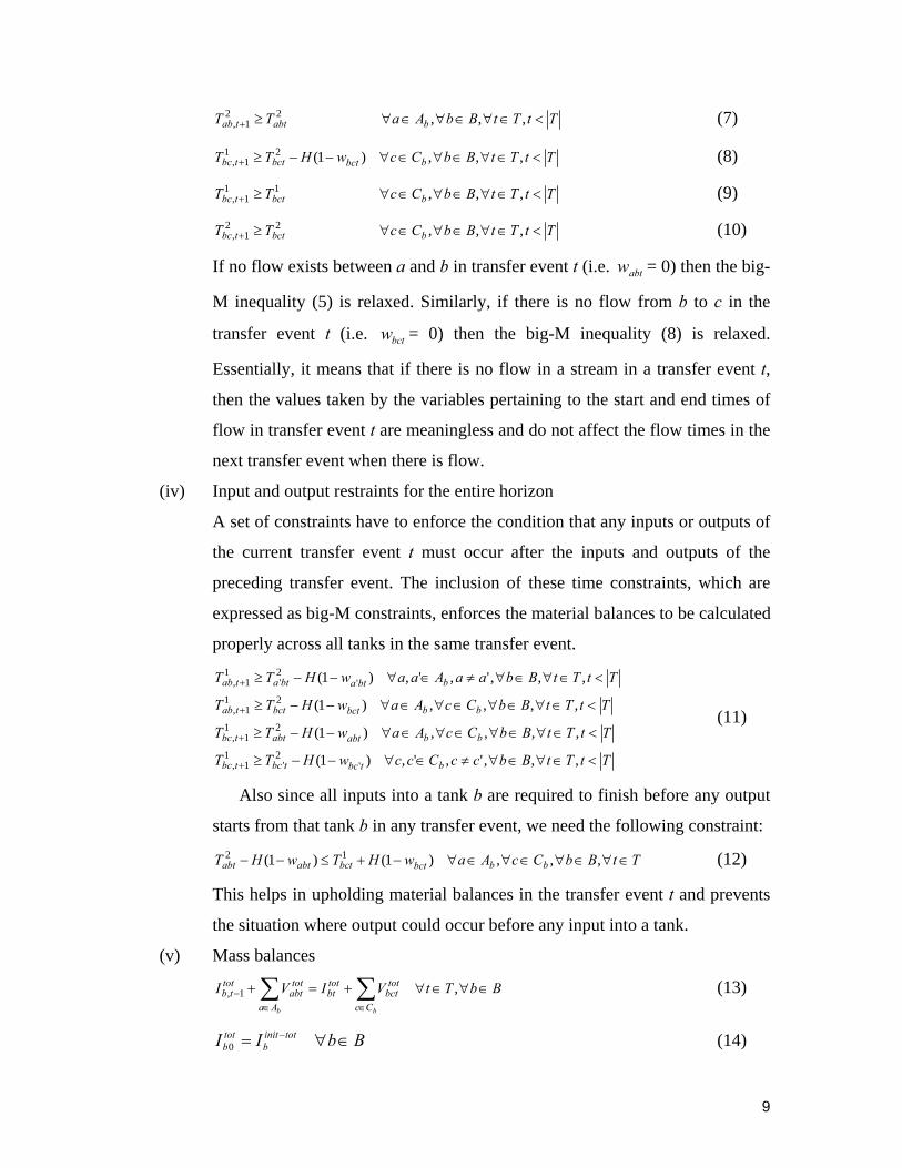
9

TtTtBbAaTT babttab <∈∀∈∀∈∀≥+ ,,,221, (7)

TtTtBbCcwHTT bbctbcttbc <∈∀∈∀∈∀−−≥+ ,,,)1(211, (8)

TtTtBbCcTT bbcttbc <∈∀∈∀∈∀≥+ ,,,111, (9)

TtTtBbCcTT bbcttbc <∈∀∈∀∈∀≥+ ,,,221, (10)

If no flow exists between a and b in transfer event t (i.e. abtw = 0) then the big-

M inequality (5) is relaxed. Similarly, if there is no flow from b to c in the

transfer event t (i.e. bctw = 0) then the big-M inequality (8) is relaxed.

Essentially, it means that if there is no flow in a stream in a transfer event t,

then the values taken by the variables pertaining to the start and end times of

flow in transfer event t are meaningless and do not affect the flow times in the

next transfer event when there is flow.

(iv) Input and output restraints for the entire horizon

A set of constraints have to enforce the condition that any inputs or outputs of

the current transfer event t must occur after the inputs and outputs of the

preceding transfer event. The inclusion of these time constraints, which are

expressed as big-M constraints, enforces the material balances to be calculated

properly across all tanks in the same transfer event.

TtTtBbccCccwHTT

TtTtBbCcAawHTT

TtTtBbCcAawHTT

TtTtBbaaAaawHTT

btbctbctbc

bbabtabttbc

bbbctbcttab

bbtabtatab

<∈∀∈∀≠∈∀−−≥

<∈∀∈∀∈∀∈∀−−≥

<∈∀∈∀∈∀∈∀−−≥

<∈∀∈∀≠∈∀−−≥

+

+

+

+

,,,',',)1(

,,,,)1(

,,,,)1(

,,,',',)1(

'2

'1

1,

211,

211,

'2'

11,

(11)

Also since all inputs into a tank b are required to finish before any output

starts from that tank b in any transfer event, we need the following constraint:

TtBbCcAawHTwHT bbbctbctabtabt ∈∀∈∀∈∀∈∀−+≤−− ,,,)1()1( 12 (12)

This helps in upholding material balances in the transfer event t and prevents

the situation where output could occur before any input into a tank.

(v) Mass balances

BbTtVIVIbb Cc

totbct

totbt

Aa

totabt

tottb ∈∀∈∀+=+ ∑∑

∈∈− ,1, (13)

BbII totinitb

totb ∈∀= −

0 (14)

10

BbTtJjVIVIbb Cc

jbctjbtAa

jabttjb ∈∀∈∀∈∀+=+ ∑∑∈∈

− ,,1, (15)

BbJjII initjbjb ∈∀∈∀= ,0 (16)

BbTtAaVV bJj

jabttot

abt ∈∀∈∀∈∀=∑∈

,, (17)

BbTtCcVV bJj

jbcttot

bct ∈∀∈∀∈∀=∑∈

,, (18)

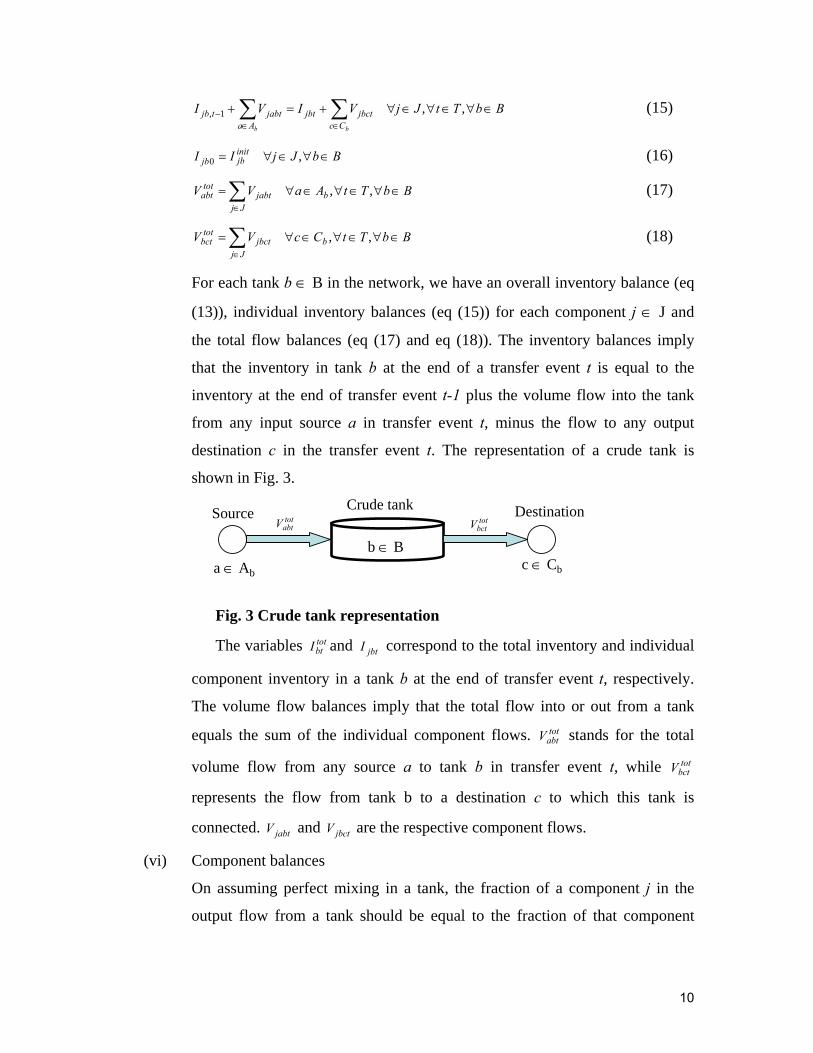
For each tank b ∈ B in the network, we have an overall inventory balance (eq

(13)), individual inventory balances (eq (15)) for each component j ∈ J and

the total flow balances (eq (17) and eq (18)). The inventory balances imply

that the inventory in tank b at the end of a transfer event t is equal to the

inventory at the end of transfer event t-1 plus the volume flow into the tank

from any input source a in transfer event t, minus the flow to any output

destination c in the transfer event t. The representation of a crude tank is

shown in Fig. 3.

Fig. 3 Crude tank representation

The variables totbtI and jbtI correspond to the total inventory and individual

component inventory in a tank b at the end of transfer event t, respectively.

The volume flow balances imply that the total flow into or out from a tank

equals the sum of the individual component flows. totabtV stands for the total

volume flow from any source a to tank b in transfer event t, while totbctV

represents the flow from tank b to a destination c to which this tank is

connected. jabtV and jbctV are the respective component flows.

(vi) Component balances

On assuming perfect mixing in a tank, the fraction of a component j in the

output flow from a tank should be equal to the fraction of that component

b ∈ Ba ∈ Ab

c ∈ Cb

Source DestinationCrude tanktot

abtV totbctV

11

present inside the tank. This constraint is formulated as follows, with bilinear

terms, which give rise to the nonconvexity of the model:

BbCcTtJjVVIVVI btot

bctAa

jabttjbjbctAa

totabt

tottb

bb

∈∀∈∀∈∀∈∀⎟⎟

⎠

⎞

⎜⎜

⎝

⎛+=⎟

⎟

⎠

⎞

⎜⎜

⎝

⎛+ ∑∑

∈−

∈− ,,,1,1, (19)

(vii) Inventory bounds

The following constraint must hold in order to ensure that the total inventory

in any transfer event does not exceed the upper bound of the inventory since

both inputs and outputs can occur in the same transfer event.

TtBbIVI Ub

Aa

totabt

tottb

b

∈∀∈∀≤+ ∑∈

− ,1, (20)

The sum ( ∑∈

− +bAa

totabt

tottb VI 1, ) is the total inventory in a tank b in transfer event t

before any output flow starts to occur from the tank in the same transfer event.

(viii) Bounds on components fractions inside a tank

The fraction of a component in the crude inside any tank should lie between

given bounds. This is enforced by the following constraints:

TtBbJjIfIIf totbt

Ujbjbt

totbt

Ljb ∈∀∈∀∈∀≤≤ ,, (21)

TtCcBbJjVfVVf btot

bctUjbjbct

totbct

Ljb ∈∀∈∀∈∀∈∀≤≤ ,,, (22)

Ljbf and U

jbf stand for the lower and upper bounds, respectively, of the fraction

of a component j inside a tank b.

(ix) Crude-mix demand constraints

Each charging tank g ∈ G must charge a specified amount of crude-mix

over the entire scheduling horizon. This volume of crude-mix is distributed to

the different CDUs in the network.

GgDMV gDd t

totgdt

g

∈∀=∑ ∑∈

(23)

(x) Bound strengthening cuts (optional)

The following constraints may be added to the model in an attempt to

tighten the relaxation of the MINLP model so as to accelerate the convergence

to find the optimal solution. These are derived using a reformulation and

12

linearization technique given in Sherali and Alameddine (1992). In this we

take eq (19) and expand it to get the following equation:

BbCcTtJjVVVIVVVI bAa

totbctjabt

totbcttjb

Aajbct

totabtjbct

tottb

bb

∈∀∈∀∈∀∈∀+=+ ∑∑∈

−∈

− ,,,1,1,

(24)

Each bilinear term present in the above equation is considered and a

summation is carried out over j ∈ J for each of these bilinear terms, which

results in the following set of equations,

BbCcTtAaVVVV

BbCcTtVIVI

BbCcTtAaVVVV

BbCcTtVIVI

bbtot

bcttot

abttot

bctJj

jabt

btot

bcttot

tbtot

bctJj

tottjb

bbtot

bcttot

abtjbctJj

totabt

btot

bcttot

tbjbctJj

tottb

∈∀∈∀∈∀∈∀=

∈∀∈∀∈∀=

∈∀∈∀∈∀∈∀=

∈∀∈∀∈∀=

∑

∑

∑

∑

∈

−∈

−

∈

−∈

−

,,,

,,

,,,

,,

1,1,

1,1,

(24a)

Distillation Units

Each distillation unit d ∈ D is modeled with the following set of constraints:

(i) Allocation constraints

The conditions that each distillation unit can be charged by at most one

charging tank in a transfer event and at most one CDU can be charged

by a single charging tank in a transfer event are enforced by eq (25)

and eq (26) respectively.

TtDdwdGg

gdt ∈∀∈∀≤∑∈

,1 (25)

TtGgwgDd

gdt ∈∀∈∀≤∑∈

,1 (26)

(ii) Continuous operation constraint

Each crude distillation unit (CDU) must be operated continuously and

the total time of operation of each CDU must be equal to the time

horizon H (eq (27)). Because of the continuity required in the duration

of operation, and the requirement that only one charging tank can

13

charge a CDU over a period of time, for a CDU which is charged in

transfer event t, the next charge (in transfer event t+1) will start at the

ending time of the current transfer event t. This is enforced by eq (28)

and eq (29).

DdHTTt Gg

gdtgdtd

∈∀=−∑ ∑∈

][ 12 (27)

TtTtDdggGggwHTT ddtgdtgtgd <∈∀∈∀≠∈∀−−≥+ ,,,',',)1( '2'

11, (28)

TtTtDdggGggwHTT ddtgdtgtgd <∈∀∈∀≠∈∀−+≤+ ,,,',',)1( '2'

11, (29)

Supply Streams

The supply streams have to follow certain mass balance and timing constraints:

(i) Timing Constraints

TtSsPpwHTT

TtSsPpwHTT

ppstpstendp

ppstpststart

p

∈∀∈∀∈∀−−≥

∈∀∈∀∈∀−+≤

,,)1(

,,)1(2

1

(30)

These constraints state that all the flows from a supply stream p to

storage tank s in any transfer event must start after a particular time

( startpT ) and end before a certain time ( end

pT ). It is to be noted that

the flow from a supply stream can be split such that one or more

storage tanks are simultaneously fed by a single supply stream.

Also, two or more suppply streams can feed the same storage tank

at the same time.

(ii) Overall mass balances

The total amount of crude oil arriving in a supply stream p (given

by supplypV ), must be completely transferred to the storage tanks

over the set of all transfer events in the horizon.

PpVV pTt Ss

totpst

p

∈∀=∑∑∈ ∈

supply (31)

(iii) Component balances

14

The component flow from a supply stream p to a tank s (storage

tank) in a transfer event t is equal to the product of the total flow

from that supply stream to the tank and the fraction of the

component in the supply stream which is known.

TtPpSsJjVfV ptotpstjpjpst ∈∀∈∀∈∀∈∀= ,,,supply (32)

supplyjpf is the fraction of component j in the supply stream p.

Variable bounds

All the continuous variables must lie between specified bounds and the

discrete variables can be either 0 or 1.

}1,0{,

,,0

,,0

,,0

,,0

,,0

,,0

,,,0

,,,0

,

,,0

2

1

2

1

∈

∈∀≤≤

∈∀≤≤

∈∀∈∀∈∀≤≤

∈∀∈∀∈∀≤≤

∈∀∈∀∈∀≤≤

∈∀∈∀∈∀≤≤

∈∀∈∀∈∀≤≤

∈∀∈∀∈∀≤≤

∈∀∈∀∈∀∈∀≤≤

∈∀∈∀∈∀∈∀≤≤

∈∀∈∀≤≤

∈∀∈∀∈∀≤≤

bctabt

endp

arrp

startp

arrp

bbct

bbct

babt

babt

bUbc

totbct

bUab

totabt

bUbcjbct

bUabjabt

Ub

totbt

Lb

Ubjbt

ww

PpHTT

PpHTT

TtBbCcHT

TtBbCcHT

TtBbAaHT

TtBbAaHT

TtBbCcVV

TtBbAaVV

TtBbCcJjVV

TtBbAaJjVV

TtBbIII

TtBbJjII

(33)

Objective function

The objective function used in this work is similar to the one used in Lee et al.

(1996).

15

)(

)12/(2)()(

)()( zmin

NDwCset

NEIIVIbCinvH

TTCunloadTTCsea

Dd Gg tgdt

Bb

totinitb

t Tt

totbt

Aa

totabt

totbt

Pp

startp

endp

Pp

arrivalp

startp

d

b

−+

+×⎟⎟⎟

⎠

⎞

⎜⎜⎜

⎝

⎛

⎟⎟⎟

⎠

⎞

⎜⎜⎜

⎝

⎛+++×+

+−+−=

∑ ∑ ∑

∑ ∑ ∑∑

∑∑

∈ ∈

∈

−

<∈

∈∈

(34)

where ∑ −p

arrivalp

startp TTCsea )( is a waiting cost for a supply stream while the term

∑ −p

startp

endp TTCunload )( represents the unloading cost of crude for a supply stream. The

total inventory maintenance cost of all the tanks in the system is given by the

approximation )12/(2)()( +×⎟⎟⎟

⎠

⎞

⎜⎜⎜

⎝

⎛

⎟⎟⎟

⎠

⎞

⎜⎜⎜

⎝

⎛+++×∑ ∑ ∑∑

∈

−

<∈

NEIIVIbCinvHBb

totinitb

t Tt

totbt

Aa

totabt

totbt

b

. This term is

written in this way, since the model allows for both input into and output from a tank in

the same transfer event, although they cannot be simultaneous. The last term

)( NDwCsetDd Gg t

gdtd

−∑ ∑∑∈ ∈

corresponds to the setup cost of charging the ‘ND’ CDUs with

different crude-mixes.

Equations (1) – (23), (25) – (34) comprise the MINLP model (P) which is to be

optimized.

4. Solution Strategy

Large scale MINLPs such as problem (P) require specialized solution algorithms.

We propose a specialized Outer-Approximation algorithm for solving the nonconvex

model (P) to global optimality within a specified tolerance. In the proposed technique, we

generate lower and upper bounds on the global optimum of (P) over a search region by

solving separate models, which are then converged in the proposed algorithm.

4.1 Lower Bounding problem

A rigorous lower bound on the global optimum of problem (P) can be obtained by

solving an MILP relaxation of the original nonconvex MINLP model (P). This relaxation

can be constructed by replacing the nonlinear equation (19) with eq (35) and using

16

convex envelopes (see McCormick, 1976) (eqs (36) – (39)) for the bilinear terms

appearing in eq (19), as given by the constraints below,

BbCcTtJjVIVI bAa

VTjabct

VTjbct

Aa

VJjabct

VJjbct

bb

∈∀∈∀∈∀∈∀+=+ ∑∑∈∈

,,, (35)

BbTtCcjVIIVVII

BbTtCcjVIIVVII

BbTtCcjVIIVVII

BbTtCcjVIIVVII

bL

bcUb

tottb

Lbcjbct

Ub

VJjbct

bUbc

Lb

tottb

Ubcjbct

Lb

VJjbct

bUbc

Ub

tottb

Ubcjbct

Ub

VJjbct

bL

bcLb

tottb

Lbcjbct

Lb

VJjbct

∈∀∈∀∈∀∀−+≤

∈∀∈∀∈∀∀−+≤

∈∀∈∀∈∀∀−+≥

∈∀∈∀∈∀∀−+≥

−

−

−

−

,,,

,,,

,,,

,,,

1,

1,

1,

1,

(36)

BbTtCcjVIIVVII

BbTtCcjVIIVVII

BbTtCcjVIIVVII

BbTtCcjVIIVVII

bL

bcUbtjb

Lbc

totbct

Ub

VTjbct

bUbc

Lbtjb

Ubc

totbct

Lb

VTjbct

bUbc

Ubtjb

Ubc

totbct

Ub

VTjbct

bL

bcLbtjb

Lbc

totbct

Lb

VTjbct

∈∀∈∀∈∀∀−+≤

∈∀∈∀∈∀∀−+≤

∈∀∈∀∈∀∀−+≥

∈∀∈∀∈∀∀−+≥

−

−

−

−

,,,

,,,

,,,

,,,

1,

1,

1,

1,

(37)

BbTtCcAajVVVVVVV

BbTtCcAajVVVVVVV

BbTtCcAajVVVVVVV

BbTtCcAajVVVVVVV

bbL

bcUab

totabt

Lbcjbct

Uab

VJjabct

bbUbc

Lab

totabt

Ubcjbct

Lab

VJjabct

bbUbc

Uab

totabt

Ubcjbct

Uab

VJjabct

bbL

bcL

abtot

abtL

bcjbctL

abVJjabct

∈∀∈∀∈∀∈∀∀−+≤

∈∀∈∀∈∀∈∀∀−+≤

∈∀∈∀∈∀∈∀∀−+≥

∈∀∈∀∈∀∈∀∀−+≥

,,,,

,,,,

,,,,

,,,,

(38)

BbTtCcAajVVVVVVV

BbTtCcAajVVVVVVV

BbTtCcAajVVVVVVV

BbTtCcAajVVVVVVV

bbL

bcUabjabt

Lbc

totbct

Uab

VTjabct

bbUbc

Labjabt

Ubc

totbct

Lab

VTjabct

bbUbc

Uabjabt

Ubc

totbct

Uab

VTjabct

bbL

bcL

abjabtL

bctot

bctL

abVTjabct

∈∀∈∀∈∀∈∀∀−+≤

∈∀∈∀∈∀∈∀∀−+≤

∈∀∈∀∈∀∈∀∀−+≥

∈∀∈∀∈∀∈∀∀−+≥

,,,,

,,,,

,,,,

,,,,

(39)

The relaxed MILP problem (R) consists of eqs (1) – (18), (20) – (23), (25) – (39).

The MILP relaxation (R) is often very large in size and requires significant computational

effort to solve. To reduce the computational effort in solving this problem, we add cutting

planes to model (R) which are derived using a technique, similar to that given in

Karuppiah and Grossmann (2006). The description of the derivation of these cutting

planes follows. The network is split into separate decoupled structures, as shown in Fig.

3, following the concept of spatial decomposition (e.g. see Jackson and Grossmann,

2003). Here the network is split into two decoupled sub-structures, although more sub-

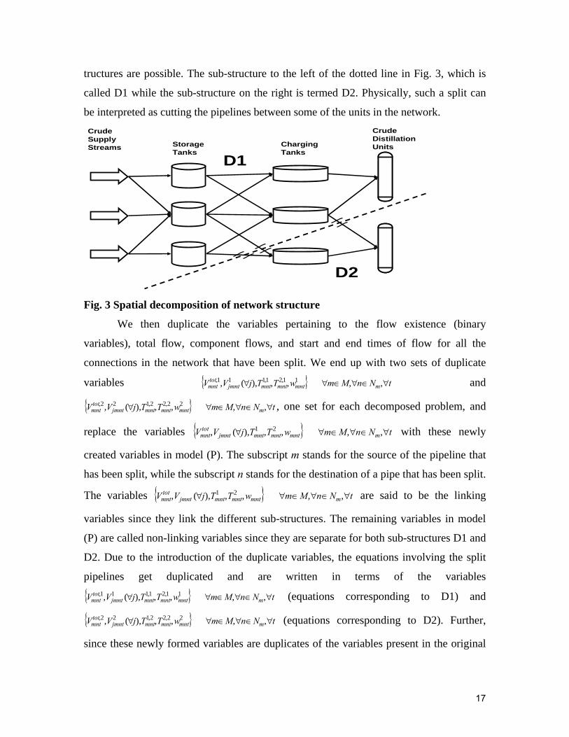
17

tructures are possible. The sub-structure to the left of the dotted line in Fig. 3, which is

called D1 while the sub-structure on the right is termed D2. Physically, such a split can

be interpreted as cutting the pipelines between some of the units in the network.

Fig. 3 Spatial decomposition of network structure

We then duplicate the variables pertaining to the flow existence (binary

variables), total flow, component flows, and start and end times of flow for all the

connections in the network that have been split. We end up with two sets of duplicate

variables { } tNnMmwTTjVV mmntmntmntjmnttotmnt ∀∈∀∈∀∀ ,,,,),(, 11,21,111, and

{ } tNnMmwTTjVV mmntmntmntjmnttotmnt ∀∈∀∈∀∀ ,,,,),(, 22,22,122, , one set for each decomposed problem, and

replace the variables { } tNnMmwTTjVV mmntmntmntjmnttotmnt ∀∈∀∈∀∀ ,,,,),(, 21 with these newly

created variables in model (P). The subscript m stands for the source of the pipeline that

has been split, while the subscript n stands for the destination of a pipe that has been split.

The variables { } tNnMmwTTjVV mmntmntmntjmnttotmnt ∀∈∀∈∀∀ ,,,,),(, 21 are said to be the linking

variables since they link the different sub-structures. The remaining variables in model

(P) are called non-linking variables since they are separate for both sub-structures D1 and

D2. Due to the introduction of the duplicate variables, the equations involving the split

pipelines get duplicated and are written in terms of the variables

{ } tNnMmwTTjVV mmntmntmntjmnttotmnt ∀∈∀∈∀∀ ,,,,),(, 11,21,111, (equations corresponding to D1) and

{ } tNnMmwTTjVV mmntmntmntjmnttotmnt ∀∈∀∈∀∀ ,,,,),(, 22,22,122, (equations corresponding to D2). Further,

since these newly formed variables are duplicates of the variables present in the original

D1

D2

Crude Supply Streams Storage

TanksCharging Tanks


18

model, they are related by the following equality constraints which are added to model

(P):

TtNnMmVV mtot

mnttot

mnt ∈∀∈∀∈∀=− ,,02,1, (40)

TtNnMmJjVV mjmntjmnt ∈∀∈∀∈∀∈∀=− ,,,021 (41)

TtNnMmTT mmntmnt ∈∀∈∀∈∀=− ,,02,11,1 (42)

TtNnMmTT mmntmnt ∈∀∈∀∈∀=− ,,02,21,2 (43)

TtNnMmww mmntmnt ∈∀∈∀∈∀=− ,,021 (44)

Equations (40) – (44) are then dualized, that is, they are multiplied by the Lagrange

multipliers 21 ,),(, Tmnt

Tmnt

VCjmnt

Vtotmnt j λλλλ ∀ and w

mntλ tNnMm m ∀∈∀∈∀ ,, , respectively, and

transferred to the objective function. This yields a Lagrangean relaxation of the original

problem, which is denoted by (LRP), and is decomposable into smaller sub-problems

corresponding to D1 and D2, which are easier to solve.

The model (LRP) is decomposed into two smaller sub-problems (LD1) and (LD2)

such that model (LD1) includes equations and variables pertaining to structure D1, while

model (LD2) includes equations and variables corresponding to the structure D2. The

bounds of all the non-linking variables in both the sub-problems are the same as in the

original full space problem (P). For the case of the duplicate variables, their bounds are

the same as the bounds of the corresponding linking variables in the original problem.

The two models (LD1) and (LD2) are as follows:

D1in sconnectionand units toingcorrespond sconstraints.t.

)(

)12/(2)()()(min

11,221,1111,

1

1

1

111

∑ ∑∑∑ ∑ ∑∑ ∑∑∑∑ ∑∑∑ ∑∑

∑ ∑∑

∑ ∑ ∑∑∑∑

∈ ∈∈ ∈∈ ∈∈ ∈∈ ∈

∈ ∈

∈

−

<∈∈∈

++++

+−+

+×⎟⎟⎟

⎠

⎞

⎜⎜⎜

⎝

⎛

⎟⎟⎟

⎠

⎞

⎜⎜⎜

⎝

⎛+++×+−+−=

Mm Nn tmnt

wmnt

Mm Nn tmnt

Tmnt

Mm Nn tmnt

Tmnt

j Mm Nn tjmnt

VCjmnt

Mm Nn t

totmnt

Vtotmnt

DDd Gg t

gdt

Bb

totinitb

t Tt

totbt

Aa

totabt

totbtb

Pp

startp

endp

Pp

arrivalp

startp

LD

mmmmm

D d

D bDD

wTTVV

NDwCset

NEIIVICinvHTTCunloadTTCseaz

λλλλλ

(LD1)

19

D2in sconnection and units toingcorrespond sconstraints.t.

)(

)12/(2)()()(min

22,222,1122,

2

2

2

222

∑ ∑∑∑ ∑∑∑ ∑∑∑∑ ∑∑∑ ∑∑

∑ ∑∑

∑ ∑ ∑∑∑∑

∈ ∈∈ ∈∈ ∈∈ ∈∈ ∈

∈ ∈

∈

−

<∈∈∈

−−−−−

+−+

+×⎟⎟⎟

⎠

⎞

⎜⎜⎜

⎝

⎛

⎟⎟⎟

⎠

⎞

⎜⎜⎜

⎝

⎛+++×+−+−=

Mm Nn tmnt

wmnt

Mm Nn tmnt

Tmnt

Mm Nn tmnt

Tmnt

j Mm Nn tjmnt

VCjmnt

Mm Nn t

totmnt

Vtotmnt

DDd Gg t

gdt

Bb

totinitb

t Tt

totbt

Aa

totabt

totbtb

Pp

startp

endp

Pp

arrivalp

startp

LD

mmmmm

D d

D bDD

wTTVV

NDwCset


λλλλλ

(LD2)

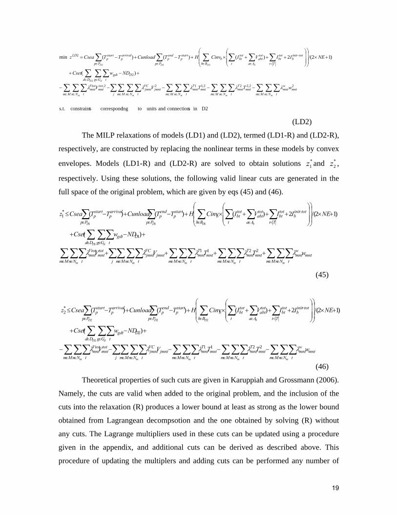
The MILP relaxations of models (LD1) and (LD2), termed (LD1-R) and (LD2-R),

respectively, are constructed by replacing the nonlinear terms in these models by convex

envelopes. Models (LD1-R) and (LD2-R) are solved to obtain solutions *1z and *

2z ,

respectively. Using these solutions, the following valid linear cuts are generated in the

full space of the original problem, which are given by eqs (45) and (46).

∑∑∑∑∑∑∑∑∑∑∑∑∑∑∑∑

∑∑∑

∑ ∑ ∑∑∑∑

∈ ∈∈ ∈∈ ∈∈ ∈∈ ∈

∈ ∈

∈

−

<∈∈∈

++++

+−+

+×⎟⎟⎟

⎠

⎞

⎜⎜⎜

⎝

⎛

⎟⎟⎟

⎠

⎞

⎜⎜⎜

⎝

⎛+++×+−+−≤

Mm Nn tmnt

wmnt

Mm Nn tmnt

Tmnt

Mm Nn tmnt

Tmnt

j Mm Nn tjmnt

VCjmnt

Mm Nn t

totmnt

Vtotmnt

DDd Gg t

gdt

Bb

totinitb

t Tt

totbt

Aa

totabt

totbtb

Pp

startp

endp

Pp

arrivalp

startp

mmmmm

D d

D bDD

wTTVV

NDwCset


λλλλλ 2211

1

*1

)(

)12/(2)()()(

1

111

(45)

∑∑∑∑∑∑∑∑∑∑∑∑∑∑∑∑

∑∑∑

∑ ∑ ∑∑∑∑

∈ ∈∈ ∈∈ ∈∈ ∈∈ ∈

∈ ∈

∈

−

<∈∈∈

−−−−−

+−+

+×⎟⎟⎟

⎠

⎞

⎜⎜⎜

⎝

⎛

⎟⎟⎟

⎠

⎞

⎜⎜⎜

⎝

⎛+++×+−+−≤

Mm Nn tmnt

wmnt

Mm Nn tmnt

Tmnt

Mm Nn tmnt

Tmnt

j Mm Nn tjmnt

VCjmnt

Mm Nn t

totmnt

Vtotmnt

DDd Gg t

gdt

Bb

totinitb

t Tt

totbt

Aa

totabt

totbtb

Pp

startp

endp

Pp

arrivalp

startp

mmmmm

D d

D bDD

wTTVV

NDwCset


λλλλλ 2211

2

*2

)(

)12/(2)()()(

2

222

(46)

Theoretical properties of such cuts are given in Karuppiah and Grossmann (2006).

Namely, the cuts are valid when added to the original problem, and the inclusion of the

cuts into the relaxation (R) produces a lower bound at least as strong as the lower bound

obtained from Lagrangean decompsotion and the one obtained by solving (R) without

any cuts. The Lagrange multipliers used in these cuts can be updated using a procedure

given in the appendix, and additional cuts can be derived as described above. This

procedure of updating the multiplers and adding cuts can be performed any number of

20

times. It is important to note that the performance of these cuts in reducing the solution

time of the relaxation strongly depends on the values of the Lagrange multipliers. The

cuts (eqs (45) and/or (46)) are then added to (R) which is the MILP relaxation of model

(P) to get a modified MILP model (RP). On solving (RP), we obtain a valid lower bound

on the solution of (P).

4.2 Upper Bounding Sub-problem

We fix the binary variables in problem (P) to the values obtained from the

solution of (RP), and obtain a nonconvex NLP model (P-NLP) which is solved to global

optimality with any standard method. This then yields an upper bound on the solution of

(P). The optimal values of the variables obtained from the solution of (RP) are then used

as a starting point for the NLP solver. In case the model (P-NLP) is found to be infeasible

for these integer values, we use as a heuristic to obtain alternate sub-optimal integer

solutions by solving (RP) for an specified amount of time, and select the best found

integer solution.

4.3 Outer Approximation Algorithm

The proposed Outer Approximation algorithm is shown in flowchart form in Fig. 4.

Fig. 4 Proposed Outer Approximation algorithm

Preprocessing

Bound Contraction optional

Solve Lower BoundingProblem

Solve Upper BoundingProblem

UB – LB ≤ tolerance ?STOP

Solution = UB

Add Integer Cuts

No Yes

21

The algorithm is along the lines of the techniques proposed by Duran and Grossmann

(1986), Kesavan et al. (2004), and Wei et al. (2005) and is outlined as follows:

a. Preprocessing The bounds of the variables in the model are determined by physical

inspection of the network structure and using the numerical data given for the tanks,

supply streams and the distillation units. Also, in this step, the original nonconvex

MINLP may be locally optimized to obtain an initial overall upper bound (OUB) for the

objective function.

b. Bound Contraction (Optional) The bounds of variables appearing in the nonconvex

terms maybe contracted by solving a set of LPs using a procedure given in Zamora and

Grossmann (1999), or the range reduction techniques in Tawarmalani and Sahinidis

(2002).

c. Lower Bound Generation Generate a valid lower bound for the solution of the

nonconvex MINLP following the technique outlined in section 4.1.

d. Upper Bound Generation Generate an upper bound using the method given in section

4.2 and update the OUB if the current upper bound is found to be better than the existing

OUB.

e. Integer Cuts Using the integer solution obtained from solving (RP), add an integer cut

to model (RP) to exclude this particular combination of binary variables. It is important

to note that if the model (P-NLP) is not globally optimized in step d, adding these integer

cuts to the relaxation in the next iteration could potentially cut off the global optimum.

f. Termination Iterate between solving models (RP) and (P-NLP) till the lower bound

exceeds the upper bound or the relaxation gap between the lower and upper bounds is

less than a specified tolerance. Convergence to the global optimum is not guaranteed if a

local NLP solver is used in step d above.

Remarks

(i) In a more traditional Lagrangean decomposition approach, the network is

usually decomposed such that all the units present in it are separated. On

solving the sub-models corresponding to every unit in the network, we obtain

very weak cuts. To avoid this problem, we decompose the network into only

22

two or three sub-structures. It is found heuristically that decomposing the

network into unbalanced sub-structures and using cuts derived from the

smaller sub-structures leads to a better performance of the algorithm.

(ii) There are multiple ways to split the network and generate sub-structures and

corresponding cutting planes. For example, the structure shown in Fig. 1 can

also be split into two sub-structures D3 and D4 as shown below in Fig. 5. Also

the original network structure can be split into more than two sub-structures.

Fig. 5 Alternate decomposition scheme for network in Fig. 1

(iii) A proposed heuristic rule on how to split the original structure is as follows:

(a) Count the number of binary variables (nb) and constraints (nc) in the

original MINLP model (P) pertaining to the optimization of the whole

network structure.

(b) Pick the largest sub-structure resulting from the proposed split scheme

and count the number of binary variables (nbs) and constraints (ncs) in the

MINLP model corresponding to this sub-structure .

(c) Calculate the ratio : (nbs + ncs)/(nb + nc) and check if it is less than 0.9. If

this condition fails, the original structure has to be split differently into

D3

D4Crude Distillation Units

Crude Supply Streams

StorageTanks

Charging Tanks

23

sub-structures such that (nbs + ncs)/(nb + nc) for the largest sub-structure

is below 0.9.

5. Examples

The effectiveness of the proposed algorithm in solving scheduling problems is

demonstrated using three examples for which the data is obtained from Lee et al. (1996).

The units of some of the parameters are not specified in order to be consistent with the

previous literature data. All examples were formulated using GAMS (Brooke et al., 1998)

and solved on Intel 3.2 GHz Linux machine with 1024 MB memory. GAMS/CPLEX 9.0

was used for solving the MILP problems, while GAMS/CONOPT 3.0 and

GAMS/BARON 7.2.5 were used for local optimization and global optimization,

respectively, of the NLP problems. For comparison with the proposed algorithm, we also

used GAMS/DICOPT and GAMS/BARON 7.2.5 for solving the MINLP models. Locally

optimal solutions to the MINLP models are obtained using DICOPT (1 iteration for the

relaxed NLP + 2 major iterations are performed) and compared against the solutions

obtained from the proposed algorithm. Hence, the computational expense of solving the

examples using DICOPT is not included in the total computational time taken by the

algorithm. It is to be noted that when BARON (Sahinidis, 1996) was used to solve the

NLP model (P-NLP), an optimality tolerance of 1% was used. The algorithm was

terminated at the end of the first iteration for all the examples, since the relaxation gap

between the lower and upper bound was sufficiently small within an acceptable tolerance

for the global optimum. However, the iterations of the proposed Outer-Approximation

algorithm may be continued to further reduce the gap between the lower and upper

bounds. The problem sizes for all three examples is given in Table 4 and the various

computational results are given in Tables 5a – 5d. The number of transfer events was

arbitrarily chosen to be 3 for all the units in all the examples, as the algorithm was able to

find good solutions when the horizon was divided into 3 transfer events.

Example 1 The first example is a network consisting of 3 supply streams, 3 storage tanks,

3 charging tanks and 2 distillation units, whose structure is shown in Fig. 1. The crude oil

24

in this example contains one key component and all the other components are combined

into a bulk component, thus effectively making the given crude a two component system.

The crude movement has to be scheduled over a time horizon of 12 hours. The relevant

numerical data to carry out the optimization for this example is given in Table 1.

Table 1. Data for example 1

Scheduling Horizon (H) 12 hours

Number of crude supply

streams 3

Crude Supply

Stream

Arrival time

( arrpT )

Incoming

volume of crude

Fraction of key

component

IN1 1 50 0.01

IN2 5 50 0.085

IN3 9 50 0.06

Number of Storage Tanks 3

Storage

Tank Capacity Initial Oil Inventory

Initial fraction of

key component (min – max)

ST1 100 20 0.02 (0.01 – 0.03)

ST2 100 20 0.05 (0.04 – 0.06)

ST3 100 20 0.08 (0.07 – 0.09)

Number of Charging Tanks 3

Charging

Tank Capacity Initial Oil Inventory

Initial fraction of


CT1 100 30 0.03 (0.025 – 0.035)

CT2 100 50 0.05 (0.045 – 0.065)

CT3 100 30 0.08 (0.075 – 0.085)

25

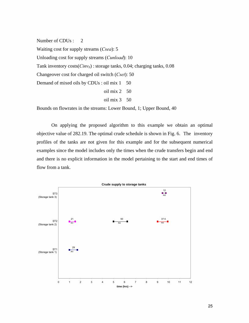
Number of CDUs : 2

Waiting cost for supply streams (Csea): 5

Unloading cost for supply streams (Cunload): 10

Tank inventory costs(Cinvb) : storage tanks, 0.04; charging tanks, 0.08

Changeover cost for charged oil switch (Cset): 50

Demand of mixed oils by CDUs : oil mix 1 50

oil mix 2 50

oil mix 3 50

Bounds on flowrates in the streams: Lower Bound, 1; Upper Bound, 40

On applying the proposed algorithm to this example we obtain an optimal

objective value of 282.19. The optimal crude schedule is shown in Fig. 6. The inventory

profiles of the tanks are not given for this example and for the subsequent numerical

examples since the model includes only the times when the crude transfers begin and end

and there is no explicit information in the model pertaining to the start and end times of

flow from a tank.

Crude supply to storage tanks

0 1 2 3 4 5 6 7 8 9 10 11 12

time (hrs) -->

ST2

ST1

ST3

IN1

IN3

IN3IN2

IN1

12.

37.55021

29

(Storage tank 3)

(Storage tank 2)

(Storage tank 1)

26

Crude transfers between storage and charging tanks

0 1 2 3 4 5 6 7 8 9 10 11 12

time (hrs) -->

CT2

CT1

CT3 12.57.

9.11

10.89

16

ST2

ST3

ST2

ST1

ST2(Charging tank 3)

(Charging tank 1)

(Charging tank 2)

Charging schedule for distillation units

0 1 2 3 4 5 6 7 8 9 10 11 12

time (hrs) -->

CT1

DU2

DU1CT1CT2

CT2 CT3

49.73 50

30 0.27 20

Distillation unit 2

Distillation unit 1

Fig. 6 Gantt chart of the schedule for example 1

27

Example 2 The second example is very similar in structure to the first example and it also

has 3 supply streams, 3 storage tanks, 3 charging tanks and 2 distillation units. The

network structure is shown in Fig. 7. Here we have two key components in the crude oil

instead of only one as in example 1. The crude in this example is hence a three

component fluid with these key components along with the remaining bulk component.

This makes the model size larger for this example.

Fig. 7 Network structure for example 2

The scheduling has to be done for a time horizon of 10 hours. Table 2 provides

the necessary data for the optimization and the optimal solution is given in Fig. 8.




streams 3

Crude Supply

Stream

Arrival time

( arrpT )

Incoming volume

of crude

Fraction of

key

component 1

Fraction of

key

component 2

IN1 1 100 0.01 0.04

IN2 4 100 0.03 0.02

IN3 7 100 0.05 0.01


StorageTanks

Charging Tanks


28


Storage

Tank Capacity

Initial Oil

Inventory

Initial fraction of key

component 1


component 2

ST1 100 20 0.01 0.04

ST2 100 50 0.03 0.02

ST3 100 70 0.05 0.01


Charging

Tank Capacity

Initial Oil

Inventory


component 1

(min – max)


component 2

(min – max)

CT1 100 30 0.0167 (0.01 – 0.02) 0.0333 (0.03 – 0.038)

CT2 100 50 0.03 (0.025 – 0.035) 0.023 (0.018 – 0.027)

CT3 100 30 0.0433 (0.04 – 0.048) 0.0133 (0.01 – 0.018)

Number of CDUs : 3



Tank inventory costs (Cinvb): storage tanks, 0.05; charging tanks, 0.08



oil mix 2 100

oil mix 3 100


29


0 1 2 3 4 5 6 7 8 9 10

time (hrs) -->

ST2

ST1

ST3IN3

IN2

IN1

100

100

100

(Storage tank 3)

(Storage tank 2)

(Storage tank 1)


0 1 2 3 4 5 6 7 8 9 10

time (hrs) -->

CT2

CT1

CT3

10.76

35.1

4.09 65.91

20

ST2

ST3

ST1

ST1

ST2

35.1

34.8ST3

ST2(Charging tank 3)

(Charging tank 2)

(Charging tank 1)

30


Distillationunit 1

Distillationunit 2

0 1 2 3 4 5 6 7 8 9 10

time (hrs) -->

CT1

DU2

DU1CT1CT2

CT2 CT3

50 100

17.61 50 82.39

Fig. 8 Optimal solution for example 2

Example 3 The final example is an industrial size problem with 3 supply streams, 6

storage tanks, 4 charging tanks and 3 distillation units. The crude oil has to be scheduled

over a time horizon of 15 hours. The crude oil in this system involves a single key

component as in example 1 and other components combined into a bulk component. The

network structure is shown in Fig. 9.

31

Fig. 9 Network structure for example 3

The relevant numerical data for this example is given in Table 3 while the optimal

schedule is shown in Fig. 10.




streams 3

Crude Supply

Stream

Arrival Time

( arrpT )

Incoming

Volume of

crude

Fraction of key

component

IN1 1 60 0.03

IN2 6 60 0.05

IN3 11 60 0.065


Storage

Tank Capacity Initial Inventory

Initial fraction of


ST1 10 – 90 60 0.031 (0.025 – 0.038)

ST2 10 – 110 10 0.03 (0.02 – 0.04)


StorageTanks

Charging Tanks


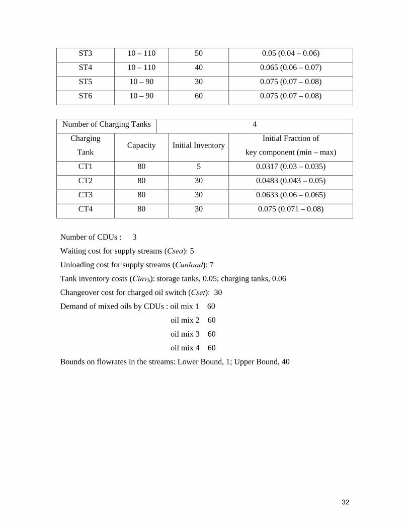
32

ST3 10 – 110 50 0.05 (0.04 – 0.06)

ST4 10 – 110 40 0.065 (0.06 – 0.07)

ST5 10 – 90 30 0.075 (0.07 – 0.08)

ST6 10 – 90 60 0.075 (0.07 – 0.08)


Charging

Tank Capacity Initial Inventory

Initial Fraction of


CT1 80 5 0.0317 (0.03 – 0.035)

CT2 80 30 0.0483 (0.043 – 0.05)

CT3 80 30 0.0633 (0.06 – 0.065)

CT4 80 30 0.075 (0.071 – 0.08)

Number of CDUs : 3



Tank inventory costs (Cinvb): storage tanks, 0.05; charging tanks, 0.06



oil mix 2 60

oil mix 3 60

oil mix 4 60


33


0 1 2 3 4 5 6 7 8 9 10 11 12 13 14 15

time (hrs) -->

ST1

ST2

ST3

ST4

ST5

ST6

IN1

IN3

IN2

IN1

60

60

555

(Storage tank 6)

(Storage tank 5)

(Storage tank 4)

(Storage tank 3)

(Storage tank 2)

(Storage tank 1)


0 1 2 3 4 5 6 7 8 9 10 11 12 13 14 15time (hrs) -->

CT3

CT2

CT4

CT1

ST6

ST5

ST4

ST3

ST2

ST150

10

20

30

30

5

(Charging tank 4)

(Charging tank 3)

(Charging tank 2)

(Charging tank 1)

34


0 1 2 3 4 5 6 7 8 9 10 11 12 13 14 15

time (hrs) -->

DU2

DU1

DU3CT4CT3CT4

CT2CT3

CT1CT2

303030

3030

6030

Distillation unit 3

Distillation unit 2

Distillation unit 1

Fig. 10 Optimal schedule for example 3

On solving the problem to optimality using the proposed algorithm, we get a

solution of 383.69, which is globally optimal within a tolerance of 1 %.

Computational results

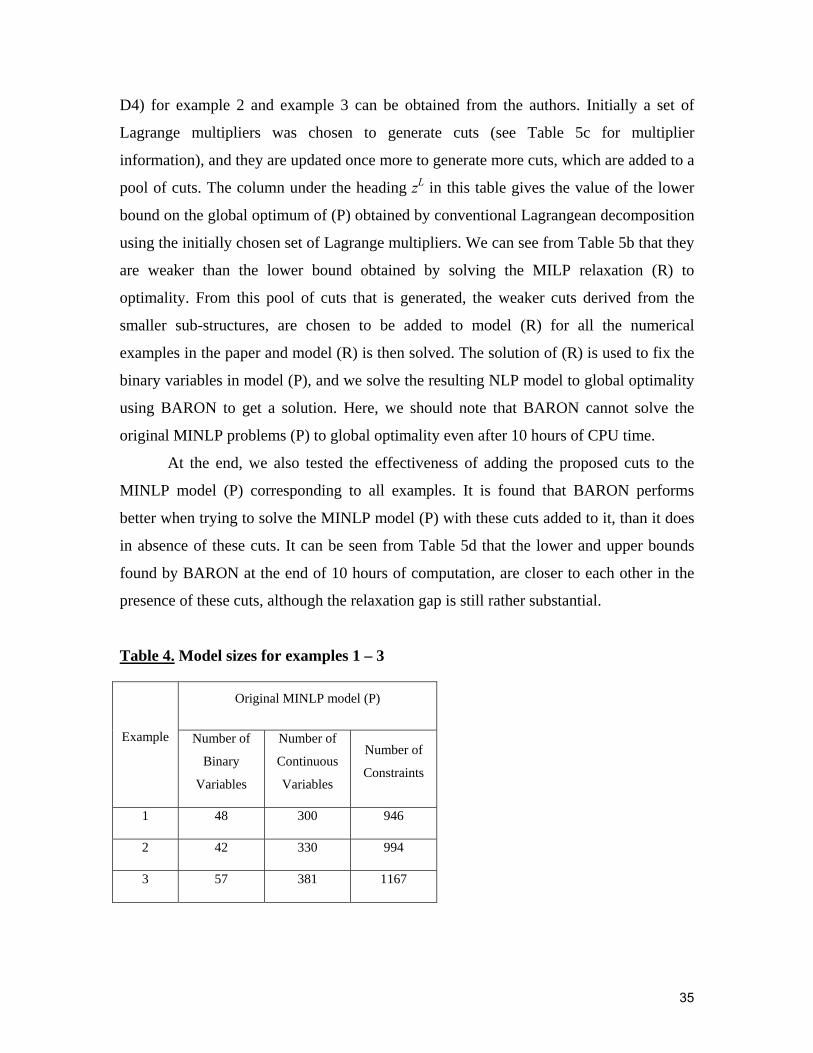
The model sizes for the different examples are shown in Table 4. The new

formulation is quite efficient for these crude oil scheduling problems and we obtain good

solutions to the scheduling problem at the very first iteration of the proposed algorithm as

seen in Table 5a. The algorithm finds the optima and proves their global optimality in

tractable computational times. The addition of cutting planes to the MILP relaxation (R)

as described in the algorithm decreases the number of nodes in the branch and bound tree

for solving the MILP relaxation, and hence the solution time for solving the MILP. This

is evident from Table 5b. The cuts added to the relaxation (R) tighten the lower bound at

the root node of the branch and bound tree for the MILP, which contributes to reducing

the number of nodes in the tree to about one third for solving the MILP.

For all the examples, the network structure is split into D1 and D2 (Fig. 2) and

also into D3 and D4 (Fig. 3). The information about the sub-structures (D1, D2, D3 and

35

D4) for example 2 and example 3 can be obtained from the authors. Initially a set of

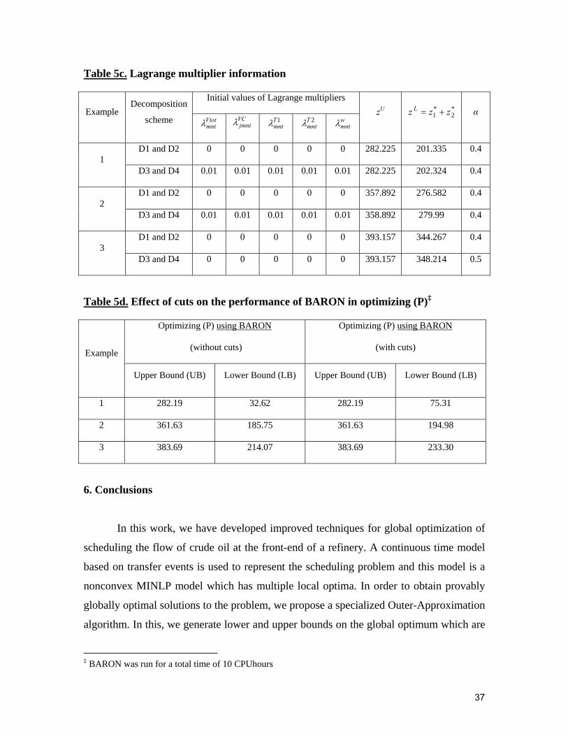
Lagrange multipliers was chosen to generate cuts (see Table 5c for multiplier

information), and they are updated once more to generate more cuts, which are added to a

pool of cuts. The column under the heading zL in this table gives the value of the lower

bound on the global optimum of (P) obtained by conventional Lagrangean decomposition

using the initially chosen set of Lagrange multipliers. We can see from Table 5b that they

are weaker than the lower bound obtained by solving the MILP relaxation (R) to

optimality. From this pool of cuts that is generated, the weaker cuts derived from the

smaller sub-structures, are chosen to be added to model (R) for all the numerical

examples in the paper and model (R) is then solved. The solution of (R) is used to fix the

binary variables in model (P), and we solve the resulting NLP model to global optimality

using BARON to get a solution. Here, we should note that BARON cannot solve the

original MINLP problems (P) to global optimality even after 10 hours of CPU time.

At the end, we also tested the effectiveness of adding the proposed cuts to the

MINLP model (P) corresponding to all examples. It is found that BARON performs

better when trying to solve the MINLP model (P) with these cuts added to it, than it does

in absence of these cuts. It can be seen from Table 5d that the lower and upper bounds

found by BARON at the end of 10 hours of computation, are closer to each other in the

presence of these cuts, although the relaxation gap is still rather substantial.

Table 4. Model sizes for examples 1 – 3

Original MINLP model (P)

Example Number of

Binary

Variables

Number of

Continuous

Variables

Number of

Constraints

1 48 300 946

2 42 330 994

3 57 381 1167

36

Table 5a. Numerical results for test examples 1 – 3

Example

Lower bound

[obtained by solving

relaxation (RP) ]

(zRP)

Upper bound

[on solving

(P-NLP) using

BARON ]

(zP-NLP)

Relaxation

gap (%)

Total time

taken for one

iteration† of

algorithm

(CPUsecs)

Local optimum

(using

DICOPT)

1 281.14 282.19 0.37 827.7 291.93

2 351.32 359.48 2.27 6913.9 361.63

3 383.69 383.69 0 8928.6 383.69

Table 5b. Comparison of relaxations with and without cuts

Solving MILP model (R) Solving MILP model (RP)

(including proposed cuts)

Example Solution

(zR)

LP

relaxation

at root

node

No. of

nodes

Time

taken to

solve (R)

(CPUsecs)

Solution

(zRP)

LP

relaxation

at root

node

No. of

nodes

Time

taken to

solve (RP)

(CPUsecs)

1 281.14 -55.24 940800 1953.3 281.14 68.45 334300 758.8

2 351.32 113.35 931700 14481.7 351.32 133.80 310600 5873.2

3 383.69 147.24 3029600 15874.8 383.69 189.19 1258100 8025.9

† Total time includes time for generating a pool of cuts, updating Lagrange multipliers, solving the relaxation (RP) using CPLEX and solving (P-NLP) using BARON

37

Table 5c. Lagrange multiplier information

Initial values of Lagrange multipliers Example

Decomposition

scheme Vtotmntλ VC

jmntλ 1Tmntλ 2T

mntλ wmntλ

zU *2

*1 zzz L += α

D1 and D2 0 0 0 0 0 282.225 201.335 0.4 1

D3 and D4 0.01 0.01 0.01 0.01 0.01 282.225 202.324 0.4

D1 and D2 0 0 0 0 0 357.892 276.582 0.4 2

D3 and D4 0.01 0.01 0.01 0.01 0.01 358.892 279.99 0.4

D1 and D2 0 0 0 0 0 393.157 344.267 0.4 3

D3 and D4 0 0 0 0 0 393.157 348.214 0.5

Table 5d. Effect of cuts on the performance of BARON in optimizing (P)‡

Optimizing (P) using BARON

(without cuts)

Optimizing (P) using BARON

(with cuts) Example

Upper Bound (UB) Lower Bound (LB) Upper Bound (UB) Lower Bound (LB)

1 282.19 32.62 282.19 75.31

2 361.63 185.75 361.63 194.98

3 383.69 214.07 383.69 233.30

6. Conclusions

In this work, we have developed improved techniques for global optimization of

scheduling the flow of crude oil at the front-end of a refinery. A continuous time model

based on transfer events is used to represent the scheduling problem and this model is a

nonconvex MINLP model which has multiple local optima. In order to obtain provably

globally optimal solutions to the problem, we propose a specialized Outer-Approximation

algorithm. In this, we generate lower and upper bounds on the global optimum which are

‡ BARON was run for a total time of 10 CPUhours

38

converged to a specified tolerance. A rigorous lower bound on the global optimum is

obtained by solving a MILP relaxation of the original problem. To reduce the

computational effort required in solving this MILP relaxation, cutting planes derived

from a spatial decomposition of the network are added to the MILP model. The solution

of the MILP is used in a heuristic to obtain a feasible solution to the MINLP, which

serves as an upper bound. The application of the proposed algorithm on different

examples helps in significantly reducing the computational effort involved in solving

such problems.

Acknowledgments

The authors gratefully acknowledge financial support from the National Science

Foundation under Grant CTS-0521769 and from ExxonMobil Research and Engineering.

Nomenclature

Indices

a tanks input source

b crude tank

c tank output destination

d distillation unit

g charging tank

j component

k node in the network

m source unit of split pipline

n destination unit of split pipeline

p supply stream

s storage tank

t transfer event

Sets

A Set of tanks input sources

39

Ab Set of inputs to a tank b

As Set of inputs to storage tank s

B Set of tanks

BD1 Set of tanks belonging to sub-structure D1

BD2 Set of tanks belonging to sub-structure D2

C Set of tank output destinations

Cb Set of outputs from a tank b

Cs Set of outputs from storage tank s

Cg Set of outputs from charging tank g

D Set of distillation units

DD1 Set of distillation units present in structure D1

DD2 Set of distillation units present in structure D2

Dg Set of distillation units that can be charged by charging tank g

G(B) Set of charging tanks

Gd Set of charging tanks that charge distillation unit d

J Set of components

K Set of nodes in the network

M Set of source units of the split pipelines

Nm Set of destination units of split pipelines with source m

P Set of supply streams

PD1 Set of supply streams present in sub-structure D1

PD2 Set of supply streams present in sub-structure D2

S(B) Set of storage tanks

Sp Set of storage tanks connected to supply stream p

T Set of transfer events

Parameters

Cinvb Inventory maintenance cost for tank b

Csea Waiting cost for supply streams

Cset Changeover cost for charged oil switch

Cunload Unloading cost for supply streams

40

UabF Upper bound on flowrate from a to b

LabF Lower bound on flowrate from a to b

Ljbf Lower bound on fraction of component j inside tank b

Ujbf Upper bound on fraction of component j inside tank b

supplyjpf Fraction of component j in supply stream p

H Time horizon for scheduling totinit

bI − Initial total inventory of tank b

initjbI Initial inventory of component j in tank b

LbI Lower bound on total inventory in a tank b

UbI Upper bound on total inventory in a tank b

ND Number of distillation units in the network

NDD1 Number of distillation units in sub-structure D1

NDD2 Number of distillation units in sub-structure D2

NE Number of transfer events arrivalpT Arrival time of crude in supply stream p

LabV Lower bound on flow from a to b L

bcV Lower bound on flow from b to c U

abV Upper bound on flow from a to b

UbcV Upper bound on flow from b to c

supplypV Total volume of crude oil arriving in supply stream p

Vtotmntλ Lagrange multiplier VCjmntλ Lagrange multiplier

1Tmntλ Lagrange multiplier

2Tmntλ Lagrange multiplier wmntλ Lagrange multiplier

41

Continuous Variables totbtI Total inventory of tank b at the end of transfer event t

jbtI Inventory of component j in tank b at the end of transfer event t

1abtT Starting time of a transfer from a to b in transfer event t

1bctT Starting time of a transfer from b to c in transfer event t

2abtT Ending time of a transfer from a to b in transfer event t

2bctT Ending time of a transfer from b to c in transfer event t

startpT Initial starting time of crude transfer from supply stream p

endpT Overall ending time of crude transfer from supply stream p

totabtV Total flow from a to b in transfer event t

totbctV Total flow from b to c in transfer event t

totjabtV Flow of component j from a from b in transfer event t

totjbctV Flow of component j from b from c in transfer event t

Binary variables

abtw Equal to 1 if there is a flow from a to b in transfer event t else 0

bctw Equal to 1 if there is a flow from b to c in transfer event t else 0

References

1. Adjiman, C. S.; Androulakis, I. P.; Floudas, C. A. (2000): Global Optimization of Mixed-Integer

Nonlinear Problems. American Institute of Chemical Engineering Journal, 46, 1769 -1797.

2. Bergamini, M. L.; Aguirre, P.; Grossmann, I. E. (2005). Logic-based outer approximation for

globally optimal synthesis of process networks. Computers and Chemical Engineering, 29, 1914 -

1933.

3. Brooke, A.; Kendrick, D.; Meeraus, A; Raman, R. (1998). GAMS: A User’s Guide, Release 2.50.

GAMS Development Corporation.

4. Duran, M. A.; Grossmann, I. E. (1986). An Outer-Approximation Algorithm for a Class of

Mixed-Integer Nonlinear Programs. Mathematical Programming, 36, 307 -339.

42

5. Fisher, M. L. (1981). The Lagrangian Relaxation Method for solving Integer Programming

Problems. Management Science, 27, 1 -18

6. Fletcher, R.; Leyffer, S. (1994). Solving Mixed Integer Nonlinear Programs by Outer

Approximation. Mathematical Programming, 66, 327 -349.

7. Floudas, C. A.; Lin, X. (2004). Continuous-Time versus Discrete-Time Approaches for

Scheduling of Chemical Processes: A Review. Computers and Chemical Engineering, 28, 2109 -

2129.

8. Furman, K. C.; Jia, Z.; Ierapetritou, M. G. (2006). A Robust Event-Based Continuous Time

Formulation for Tank Transfer Scheduling. Work in Progress.

9. Grossmann, I. E. (2002). Review of Nonlinear Mixed-Integer and Disjunctive Programming

Techniques. Optimization and Engineering, 3, 227 -252.

10. Jackson, J. R.; Grossmann, I. E. (2003). Temporal Decomposition Scheme for Nonlinear Multisite

Production Planning and Distribution Models. Industrial and Engineering Chemistry Research, 42,

3045 -3055.

11. Jia, Z.; Ierapetritou, M. G.; Kelly, J. D. (2003). Refinery Short-Term Scheduling Using

Continuous Time Formulation: Crude Oil Operations. Industrial and Engineering Chemistry

Research, 42, 3085 -3097.

12. Karuppiah, R.; Grossmann, I. E. (2006). A Lagrangean based Branch-and-Cut algorithm for global

optimization of nonconvex Mixed-Integer Nonlinear Programs with decomposable structures,

Submitted to Journal of Global Optimization.

13. Kesavan, P.; Allgor, R. J.; Gatzke, E. P.; Barton, P. I. (2004). Outer Approximation Algorithms

for Separable Nonconvex Mixed-Integer Nonlinear Programs. Mathematical Programming, 100,

517 -535.

14. Lee, H.; Pinto, J. M.; Grossmann, I. E.; Park, S. (1996). Mixed Integer Linear Programming

Model for Refinery Short-Term Scheduling of Crude Oil Unloading with Inventory Management.

Industrial and Engineering Chemistry Research, 35, 1630 -1641.

15. McCormick, G. P. (1976). Computability of Global Solutions to Factorable Nonconvex Programs

– Part I – Convex Underestimating Problems. Mathematical Programming, 10, 146 -175.

16. Mendez, C. A.; Cerda, J.; Grossmann, I. E.; Harjunkoski, I; Fahl, M. (2006). State-of-the-art

review of optimization methods for short-term scheduling of batch processes. Computers and

Chemical Engineering, 30, 913 -946.

17. Pinto, J. M.; Joly, M.; Moro, L. F. L. (2000). Planning and Scheduling Models for Refinery

Operations. Computers and Chemical Engineering, 24, 2259 -2276.

18. Sahinidis, N. (1996). BARON: A General Purpose Global Optimization Software Package.

Journal of Global Optimization, 8, 201 -205.

43

19. Shah, N. (1996). Mathematical Programming Techniques for Crude Oil Scheduling. Computers

and Chemical Engineering (Suppl.), 20, S1227 –S1232.

20. Sherali, H. D.; Alameddine, A. (1992). A New Reformulation Linearization Technique for

Bilinear Programming Problems. Journal of Global Optimization, 2, 379-410.

21. Tawarmalani, M.; Sahinidis, N. (2002). Convexification and Global Optimization in Continuous

and Mixed-Integer Nonlinear Programming: Theory, Algorithms, Software and Applications.

Kluwer Academic Publishers : Dordrecht, The Netherlands

22. Tawarmalani, M.; Sahindis, N. V. (2004). Global Optimization of Mixed-Integer Nonlinear

Programs: A Theoretical and Computational Study. Mathematical Programming, 99, 563 -591.

23. Wei, J.; Furman, K. C.; Duran, M. A.; Tawarmalani, M.; Sahinidis, N. V. (2005) Global

Optimization for Stochastic Nonconvex Mixed Integer Nonlinear Programs. IFORS 2005,

Honolulu, Hawaii.

24. Zamora, J. M.; Grossmann, I. E. (1999). A Branch and Bound Algorithm for Problems with

Concave Univariate, Bilinear and Linear Fractional Terms. Journal of Global Optimization, 14 (3),

217 -249.

Appendix : Updating Lagrange multipliers

Fisher (1981) proposed a sub-gradient method to update Lagrange multipliers, to

be used in solving a Lagrangean relaxation of the original problem, starting from an

initial arbitrary value of the multipliers. This technique is tailored to suit our problem in

order to obtain updated values of Lagrange multipliers starting with random initial

values. The generated Lagrange multipliers are then used to derive cuts to be added to the

relaxation. For solving the models (LD1-R) and (LD2-R) resulting from a decomposition

of the network structure into sub-structures D1 and D2, we succesively generate the

multipliers as follows:

[ ] [ ] ( ) ( ) TtNnMmVVts m

ktot

mnt

ktot

mntkkVtot

mntkVtot

mnt ∈∀∈∀∈∀⎥⎦

⎤⎢⎣

⎡−+=

+,,

*2,*1,1λλ

[ ] [ ] ( ) ( ) TtNnMmJjVVts m

k

jmnt

k

jmntkkVC

jmntkVC

jmnt ∈∀∈∀∈∀∈∀⎥⎦

⎤⎢⎣

⎡−+=

+,,,

*2*11λλ

[ ] [ ] ( ) ( ) TtNnMmTTts m

k

mnt

k

mntkkT

mntkT

mnt ∈∀∈∀∈∀⎥⎦

⎤⎢⎣

⎡−+=

+,,

*2,1*1,1111 λλ

[ ] [ ] ( ) ( ) TtNnMmTTts m

k

mnt

k

mntkkT

mntkT

mnt ∈∀∈∀∈∀⎥⎦

⎤⎢⎣

⎡−+=

+,,

*2,2*1,2212 λλ

44

where tsk is a scalar step size and ( ) ( ) ( ) ( ) ( )⎭⎬⎫

⎩⎨⎧

∀k

mnt

k

mnt

k

mnt

k

jmnt

ktot

mnt wTTjVV*1*1,2*1,1*1*1, ,,,, and

( ) ( ) ( ) ( ) ( )⎭⎬⎫

⎩⎨⎧

∀k

mnt

k

mnt

k

mnt

k

jmnt

ktot

mnt wTTjVV*2*2,2*2,1*2*2, ,,,, are the optimal values of the duplicate

variables, at the kth iteration, obtained from the solution of the sub-problems (LD1-R)

and (LD2-R), respectively. The following formula is used to calculate the values of tsk at

every iteration k:

( ) ( ) ( ) ( ) ( ) ( ) ( ) ( ) ( ) ( )∑ ∑∑ ∑∈ ∈ ⎥

⎥⎦

⎤

⎢⎢⎣

⎡⎟⎟⎠

⎞⎜⎜⎝

⎛−+⎟⎟

⎠

⎞⎜⎜⎝

⎛−+⎟⎟

⎠

⎞⎜⎜⎝

⎛−+⎟⎟

⎠

⎞⎜⎜⎝

⎛−+⎟⎟

⎠

⎞⎜⎜⎝

⎛−

−=

Mm Nn t

k

mnt

k

mnt

k

mnt

k

mntj

k

mnt

k

mnt

k

jmnt

k

jmnt

ktotmnt

ktotmnt

kLUkk

m

wwTTTTVVVV

zzts*2*1*2,2*1,2*2,1*1,1*2*1*2,*1,

))(( λα

where kα is a scalar chosen between 0 and 2, )( kLz λ is the sum of the obejctives of the

sub-models (LD1-R) and (LD2-R), when the multipliers are set to kλ , and zU is the value

of the best found feasible solution to (R). The parameter values used for updating the

multipliers in the numerical examples in the paper is given in Table 5c. The multiplier

update was carried out only once in this work. The updating scheme remains the same if

the network is decomposed into sub-structures D3 and D4 and the sub-models pertaining

to those are to be solved.

[ ] [ ] ( ) ( ) TtNnMmwwts m

k

mnt

k

mntkkw

mntkw

mnt ∈∀∈∀∈∀⎥⎦

⎤⎢⎣

⎡−+=

+,,

*2*11λλ

Global Optimization for Scheduling Refinery Crude Oil Operations

Documents

Transcript of Global Optimization for Scheduling Refinery Crude Oil Operations