Global Optimisation with Gaussian Processes

Michael A. Osborne Machine Learning Research Group Department o Engineering Science

University o Oxford

Global optimisation considers objective functions that are multi-modal and expensive to evaluate.

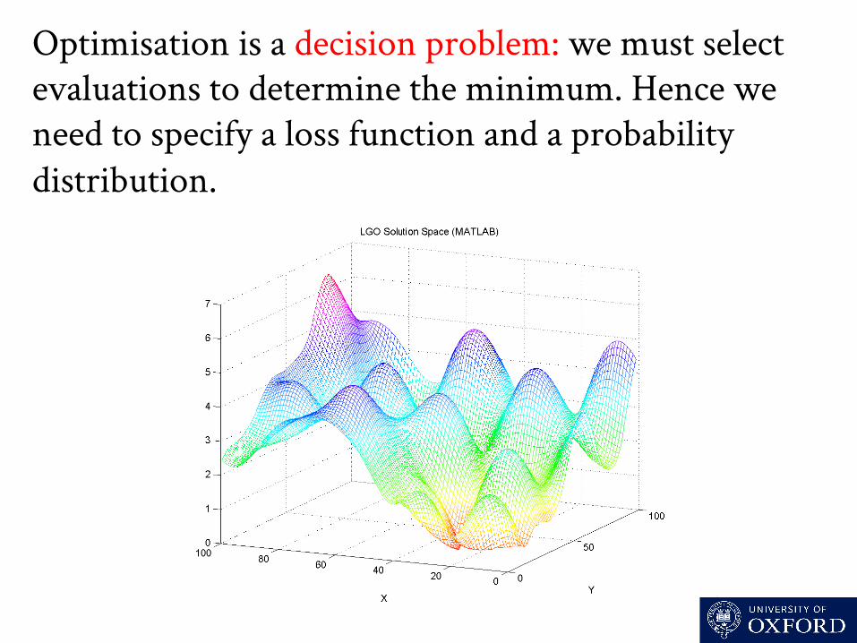
Optimisation is a decision problem: we must select evaluations to determine the minimum. Hence we need to specify a loss function and a probability distribution.

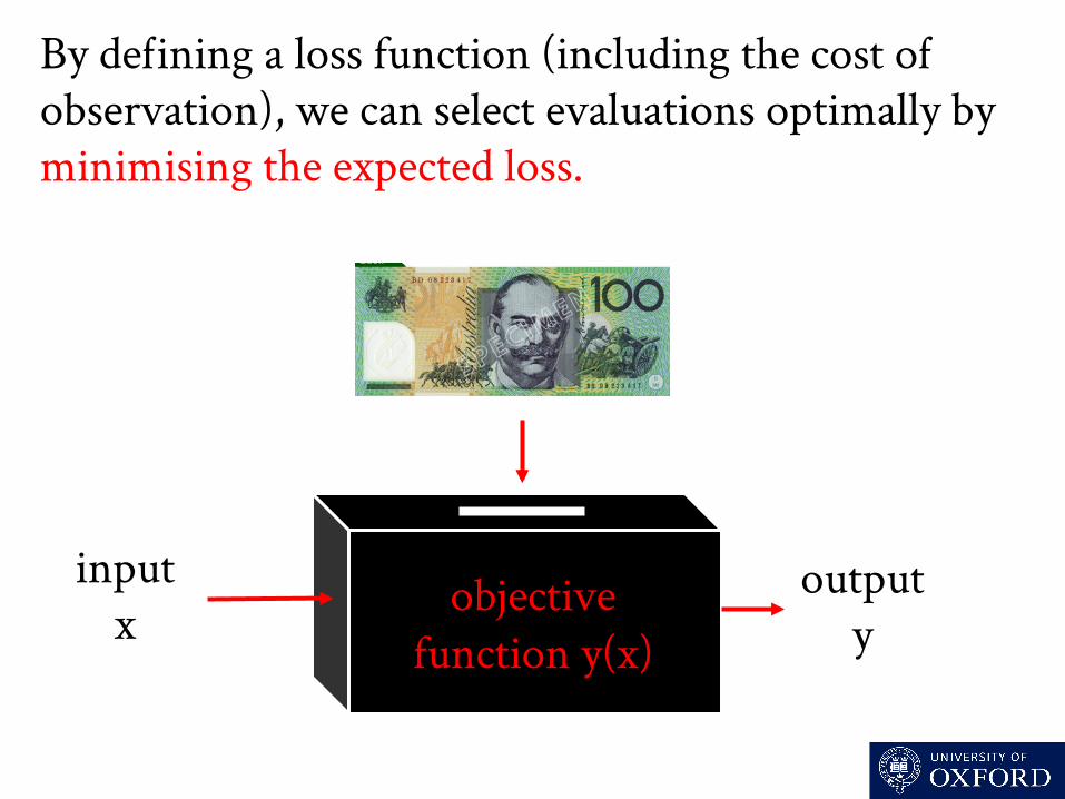
By deining a loss function (including the cost o observation), we can select evaluations optimally by minimising the expected loss.

input x

objective

function y(x) output

y

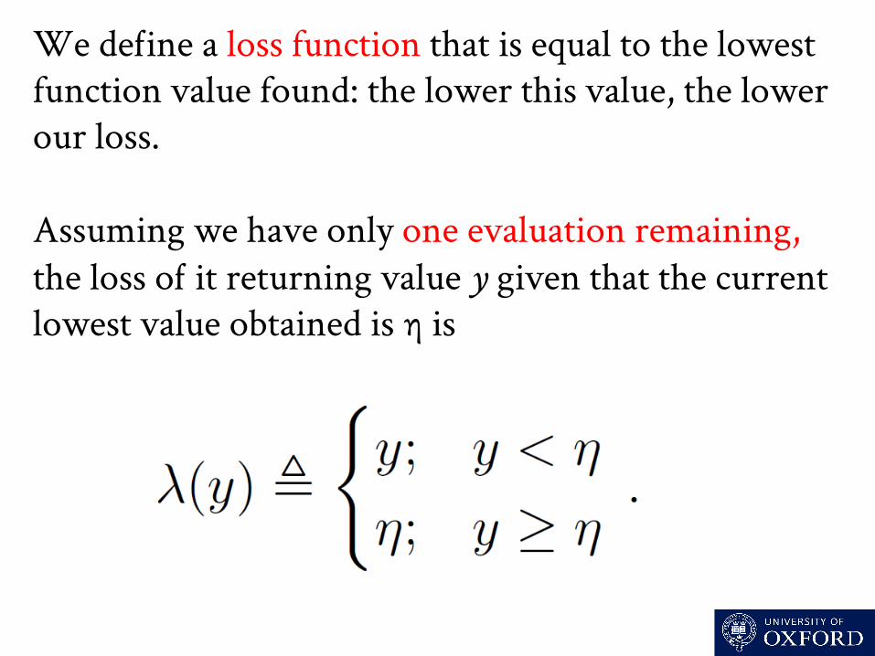
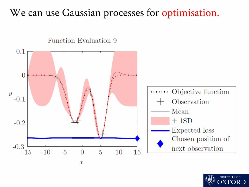
We deine a loss function that is equal to the lowest function value found: the lower this value, the lower our loss. Assuming we have only one evaluation remaining, the loss o it returning value y given that the current lowest value obtained is η is

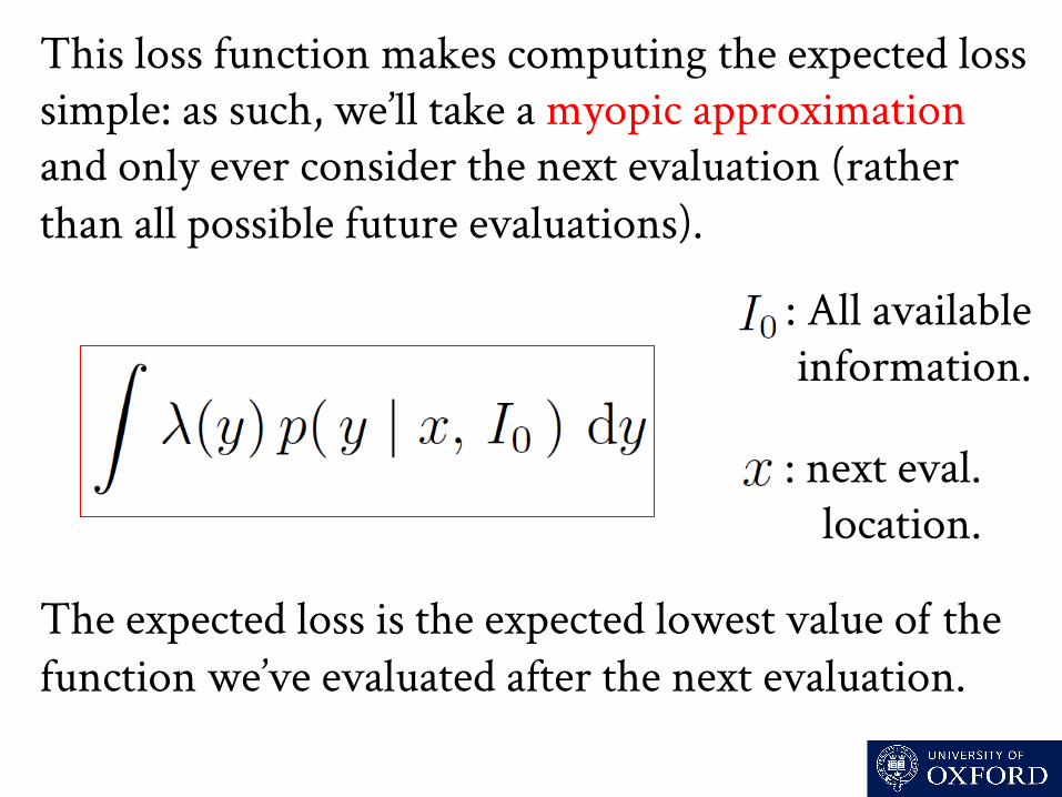
This loss function makes computing the expected loss simple: as such, we’ll take a myopic approximation and only ever consider the next evaluation (rather than all possible future evaluations). The expected loss is the expected lowest value o the function we’ve evaluated after the next evaluation.

: All available information.

: next eval. location.

We choose a Gaussian process as the probability distribution for the objective function, giving a tractable expected loss.

We can use Gaussian processes for optimisation.

We can use Gaussian processes for optimisation.

We can use Gaussian processes for optimisation.

We can use Gaussian processes for optimisation.

We can use Gaussian processes for optimisation.

We can use Gaussian processes for optimisation.

We can use Gaussian processes for optimisation.

We can use Gaussian processes for optimisation.

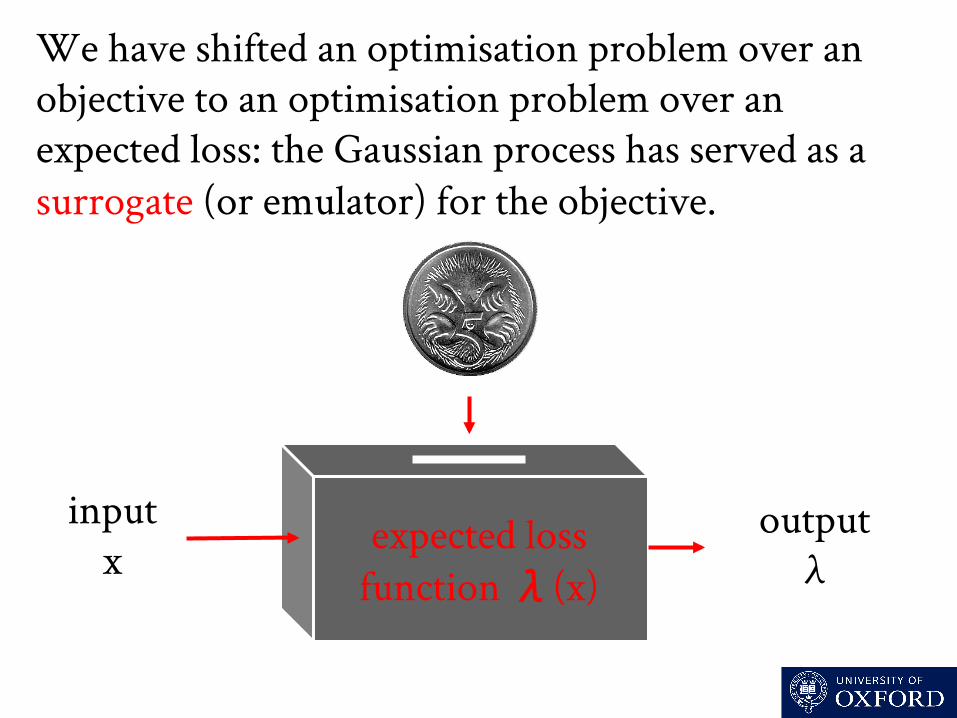
We have shifted an optimisation problem over an objective to an optimisation problem over an expected loss: the Gaussian process has served as a surrogate (or emulator) for the objective.

input x

expected loss

function λ(x) output

λ

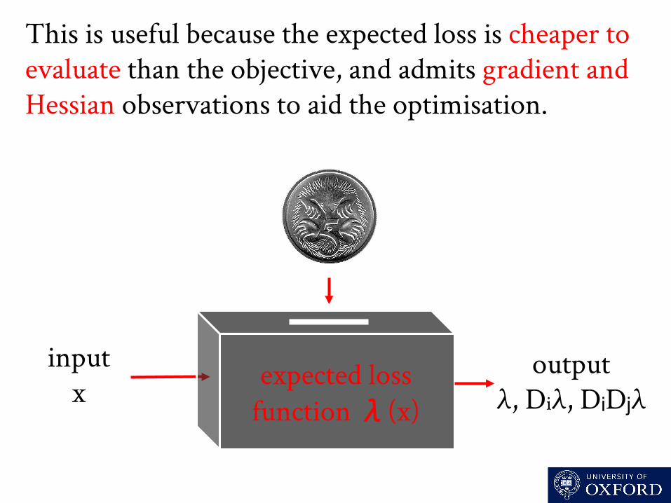
This is useful because the expected loss is cheaper to evaluate than the objective, and admits gradient and Hessian observations to aid the optimisation.

input x

expected loss

function λ(x) output

λ, Diλ, DiDjλ

λ2

Our Gaussian process is speciied by hyper-parameters λ and σ, giving expected length scales o the function in output and input spaces respectively.

σ

λ

σ

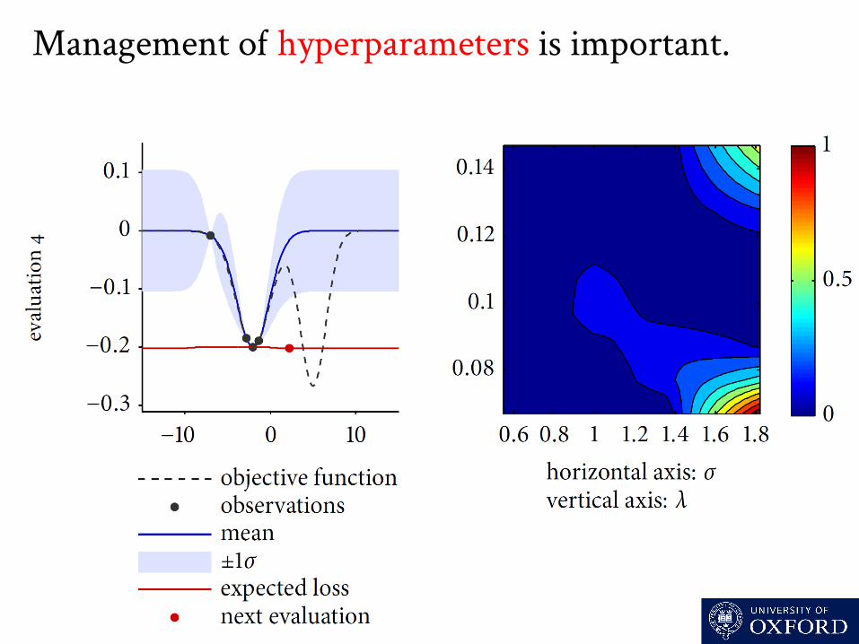
Hyperparameter values can have a signiicant inluence: below, A has small input scale and prior C has large input scale. In optimisation, amongst other things, hyperparameters specify a ‘step size’.

Management o hyperparameters is important for optimisation: we start with no data!

Management o hyperparameters is important.

Management o hyperparameters is important.

Management o hyperparameters is important.

Management o hyperparameters is important.

Management o hyperparameters is important.

Management o hyperparameters is important.

Management o hyperparameters is important.

Management o hyperparameters is important (we’ll come back to this!).

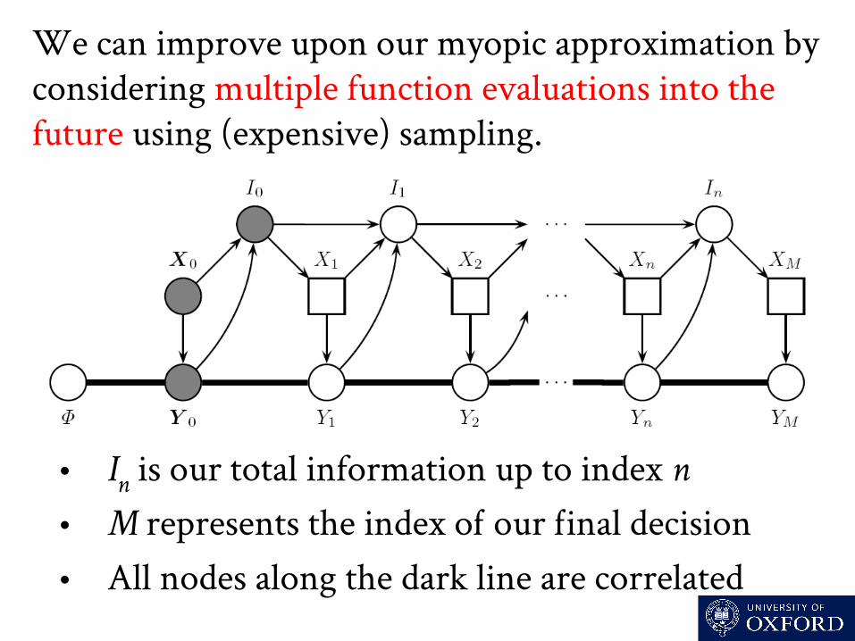
We can improve upon our myopic approximation by considering multiple function evaluations into the future using (expensive) sampling.

•  In is our total information up to index n •  M represents the index o our inal decision •  All nodes along the dark line are correlated

We tested on a range o problems. •  Ackley 2/5 •  Branin •  6-hump Camelback •  Goldstein-Price •  Griewank 2/5 •  Hartman 3/6 •  Rastigrin •  Shekel 5/7/10 •  Shubert

Gaussian process global optimisation (GPGO) outperforms tested alternatives for global optimisation over 140 test problems.

0.622 0.626 0.722

0.779

0

1

RBF DIRECT GPGO GPGO (Best)

myo

pic

2-s

tep

look

ahea

d

d/G

Start pt

True global optimum

Optimum found after set

number of fn evals

d

G

We can extend GPGO to optimise dynamic functions, by simply taking time as an additional input (that we have no control over).

We can use GPGO to select the optimal subset o sensor locations for weather prediction.

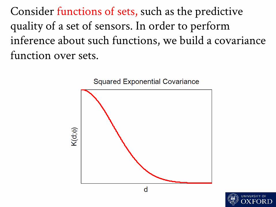
Consider functions o sets, such as the predictive quality o a set o sensors. In order to perform inference about such functions, we build a covariance function over sets.

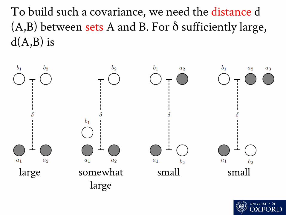
To build such a covariance, we need the distance d(A,B) between sets A and B. For δ suficiently large, d(A,B) is

large somewhat large

small small

d(A,B) is the minimum total distance that nodes would have to be moved in order to render set A identical to set B, i nodes can be ‘merged’ along the way.

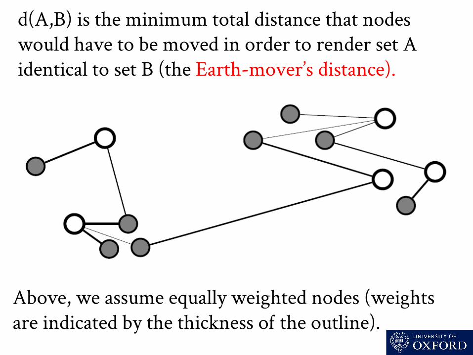
d(A,B) is the minimum total distance that nodes would have to be moved in order to render set A identical to set B (the Earth-mover’s distance).

Above, we assume equally weighted nodes (weights are indicated by the thickness o the outline).

We also wish to determine weights that relect the importance o sensors to the overall network (more isolated nodes are more important).

The mean prediction at a point given observations from set A is

This term weights the observations from A: we use it as a measure o the importance o the nodes. Note that we integrate over and normalise.

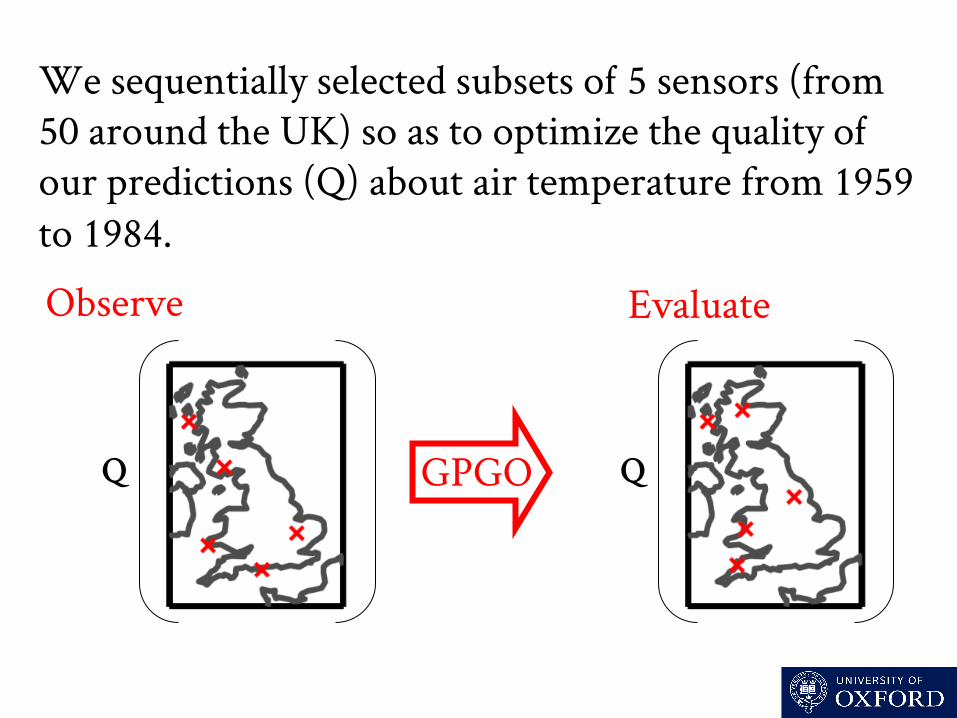
We sequentially selected subsets o 5 sensors (from 50 around the UK) so as to optimize the quality o our predictions (Q) about air temperature from 1959 to 1984.

Q Q

Observe Evaluate

GPGO

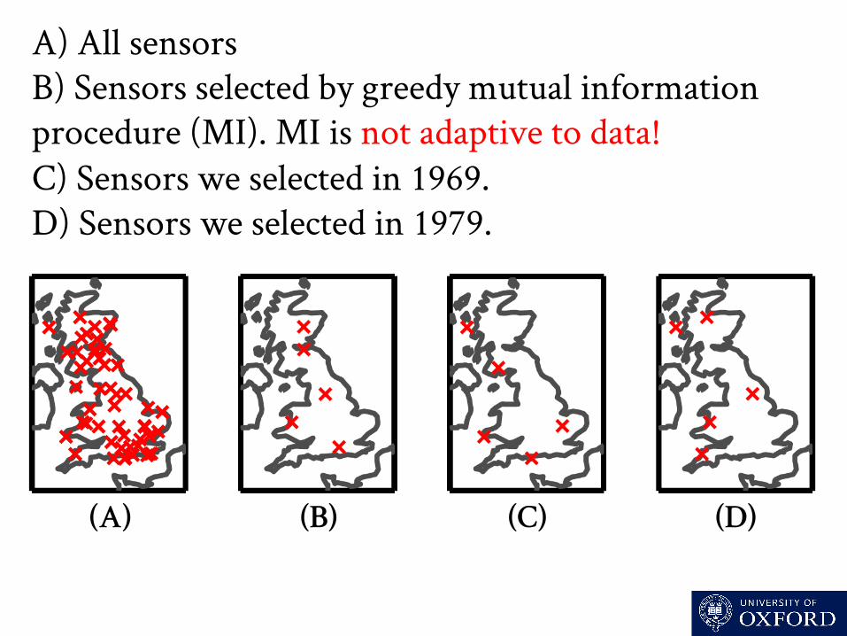
A) All sensors B) Sensors selected by greedy mutual information procedure (MI). MI is not adaptive to data! C) Sensors we selected in 1969. D) Sensors we selected in 1979.

(A) (B) (C) (D)

We could extend GPGO to additionally ind the optimal number o set elements by deining the cost o additional elements.

Gaussian distributed variables are joint Gaussian with any afine transform o them.

A function over which we have a Gaussian process is joint Gaussian with any integral or derivative o it, as integration and differentiation are afine.

( ) ( )

( ) ( )j

i

i

xxxxjiDD

xxjjiD

xxKxx

xxK

xxKx

xxK

==

=

∂

∂

∂

∂=

∂

∂=

'

, ','

,

,,derivative observation at xi and function observation at xj.

derivative observation at xi and derivative observation at xj.

We can modify covariance functions to manage derivative or integral observations.

We can modify the squared exponential covariance to manage derivative observations.

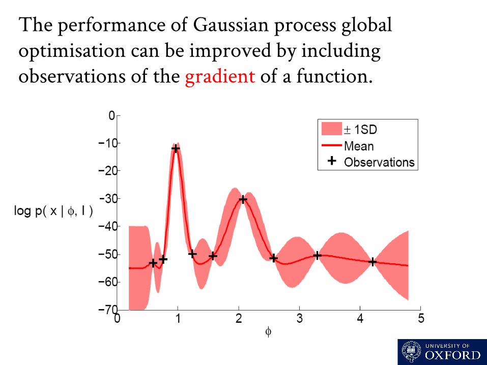
The performance o Gaussian process global optimisation can be improved by including observations o the gradient o a function.

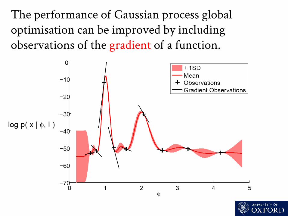
The performance o Gaussian process global optimisation can be improved by including observations o the gradient o a function.

1 0.9999 0 0 0.9999 1 0 0 0 0 1 0.1 0 0 0.1 1

Too similar

Conditioning becomes an issue when we have multiple close observations, giving rows in the covariance matrix that are very similar.

Conditioning is a particular problem in optimisation, where we often take many samples around a local minimum to exactly determine it.

1.01 0.9999 0 0 0.9999 1.01 0 0 0 0 1.01 0.1 0 0 0.1 1.01

Suciently dissimilar

The usual solution to conditioning problems is to add a small positive quantity (jitter) to the diagonal o the covariance matrix.

As jitter is effectively imposed noise, adding jitter to all diagonal elements dilutes the informativeness o our data.

We can readily incorporate observations o the derivative into the Gaussian process used in GPGO.

This also gives us a way to resolve conditioning issues (that result from the very close observations that are taken during optimisation).

We can readily incorporate observations o the derivative into the Gaussian process used in GPGO.

This also gives us a way to resolve conditioning issues (that result from the very close observations that are taken during optimisation).

We can readily incorporate observations o the derivative into the Gaussian process used in GPGO.

This also gives us a way to resolve conditioning issues (that result from the very close observations that are taken during optimisation).

We can readily incorporate observations o the derivative into the Gaussian process used in GPGO.

This also gives us a way to resolve conditioning issues (that result from the very close observations that are taken during optimisation).

We can readily incorporate observations o the derivative into the Gaussian process used in GPGO.

This also gives us a way to resolve conditioning issues (that result from the very close observations that are taken during optimisation).

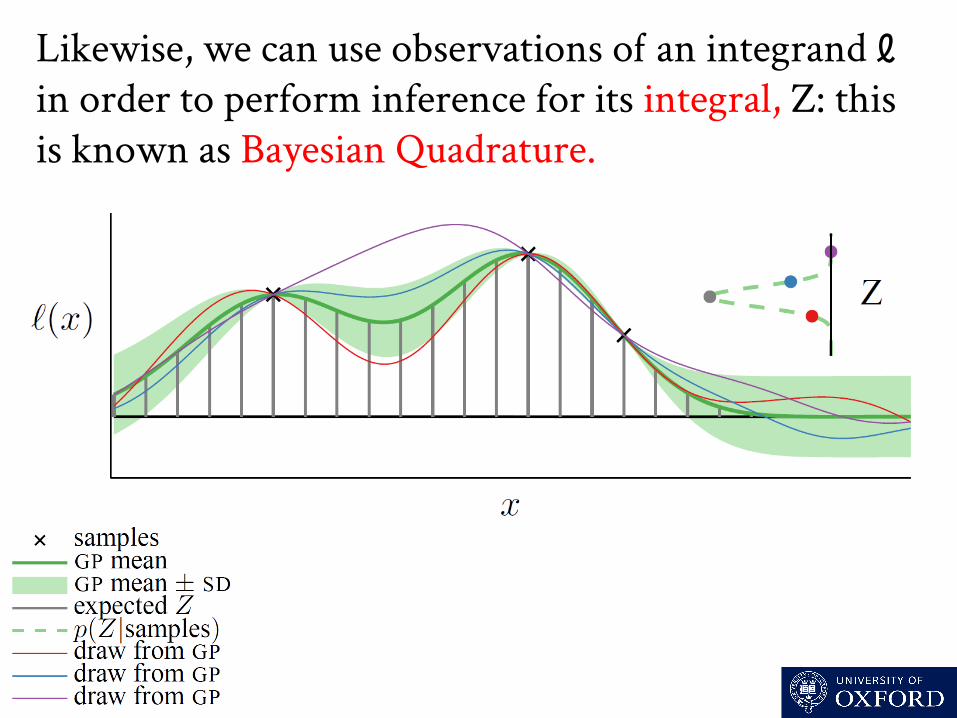
Likewise, we can use observations o an integrand ℓ in order to perform inference for its integral, Z: this is known as Bayesian Quadrature.

Modelling data is problematic due to parameters, such as the parameters o a polynomial model.

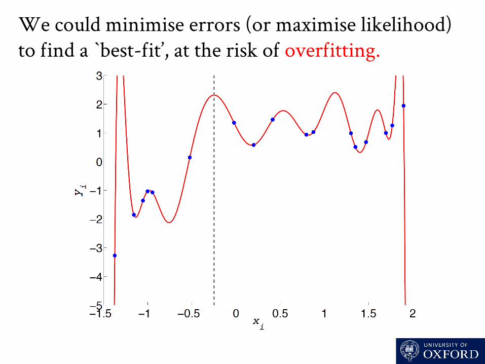
We could minimise errors (or maximise likelihood) to ind a `best-it’, at the risk o overitting.

The Bayesian approach is to average over many possible parameters, requiring integration.

The Bayesian approach is to average over many possible parameters, requiring integration.

Inference requires integrating (or marginalising) over the many possible states o the world consistent with our data, which is often non-analytic.

ϑ

Probability( y ) = the area under this curve:

Probability Density p( y, ϑ )

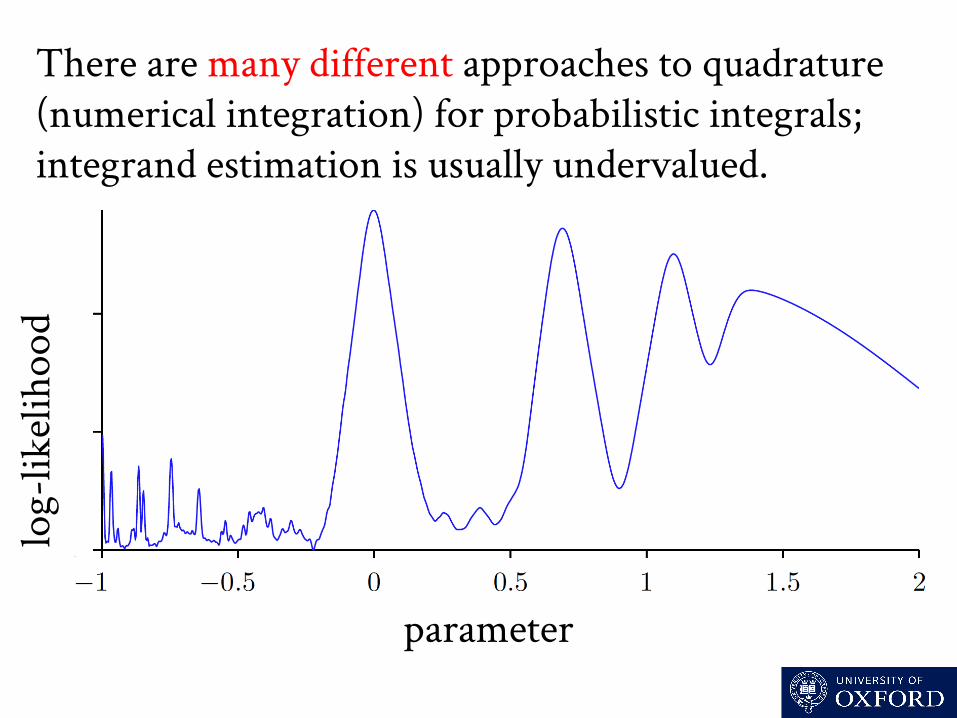
There are many different approaches to quadrature (numerical integration) for probabilistic integrals; integrand estimation is usually undervalued.

parameter

log-

likel

ihoo

d

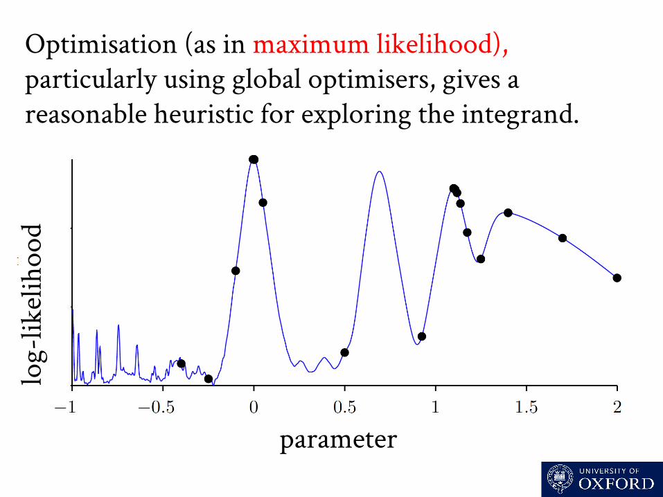
Optimisation (as in maximum likelihood), particularly using global optimisers, gives a reasonable heuristic for exploring the integrand.

parameter

log-

likel

ihoo

d

However, maximum likelihood is an unreasonable way o estimating a multi-modal or broad likelihood integrand: why throw away all those other samples?

log-

likel

ihoo

d

parameter

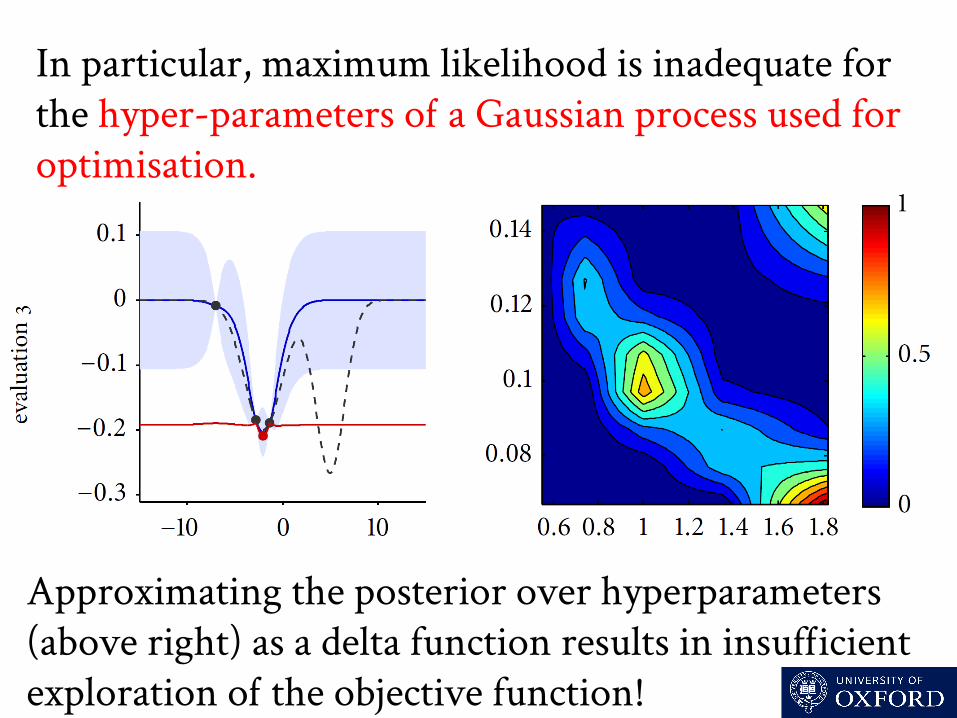
In particular, maximum likelihood is inadequate for the hyper-parameters o a Gaussian process used for optimisation.

Approximating the posterior over hyperparameters (above right) as a delta function results in insuficient exploration o the objective function!

Monte Carlo schemes give even more powerful methods o exploration, that have revolutionised Bayesian inference.

parameter

log-

likel

ihoo

d

parameter

log-

likel

ihoo

d These methods force us to be uncertain about our action, which is unlikely to result in actions that minimise a sensible expected loss.

Monte Carlo schemes give a fairly reasonable method o exploration; but an unreasonable means o integrand estimation.

parameter

log-

likel

ihoo

d

Bayesian quadrature (aka Bayesian Monte Carlo) gives a powerful method for estimating the integrand: a Gaussian process.

parameter

log-

likel

ihoo

d

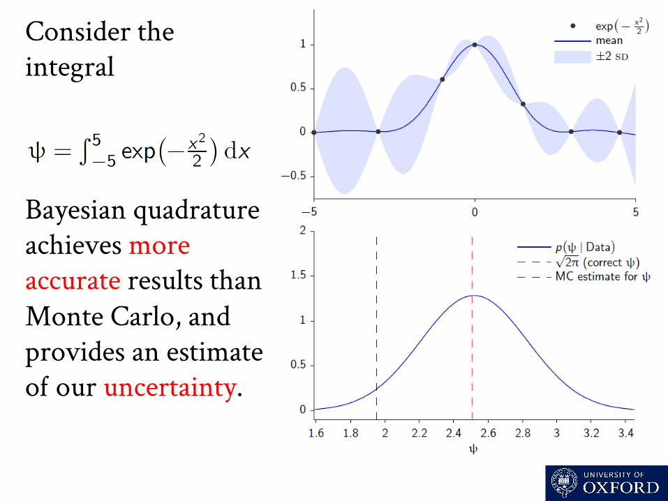
Consider the integral . Bayesian quadrature achieves more accurate results than Monte Carlo, and provides an estimate o our uncertainty.

Doubly-Bayesian quadrature (BBQ) additionally explores the integrand so as to minimise the uncertainty about the integral.

Integrand

Sample number

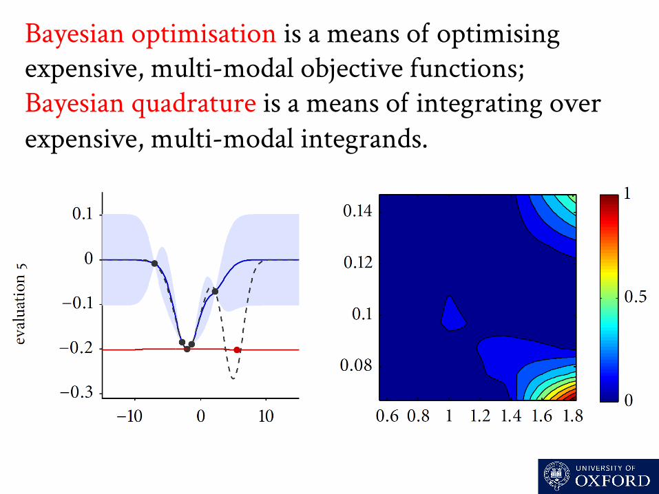
Bayesian optimisation is a means o optimising expensive, multi-modal objective functions; Bayesian quadrature is a means o integrating over expensive, multi-modal integrands.

Thanks! I would like to also like thank my collaborators: David Duvenaud, Roman Garnett, Zoubin Ghahramani, Carl Rasmussen, and Stephen Roberts. References http://www.robots.ox.ac.uk/~mosb