
Global minimum variance portfolios under uncertainty: a ...
29
1 Global minimum variance portfolios under uncertainty: a robust optimization approach Sandra Caçador a,b,c,1 [[email protected]]; Joana Matos Dias b,c,d [[email protected]]; Pedro Godinho b,c [[email protected]] a Higher Institute for Accountancy and Administration of the University of Aveiro, R. Associação Humanitária dos Bombeiros Voluntários de Aveiro, Aveiro 3810-500, Portugal b Centre for Business and Economics Research (CeBER), Faculty of Economics of the University of Coimbra, Av. Dias da Silva, 165, Coimbra 3004-512, Portugal c Faculty of Economics of the University of Coimbra, Av. Dias da Silva, 165, Coimbra 3004-512, Portugal d Institute for Systems Engineering and Computers at Coimbra, Rua Antero de Quental, Nº199, Coimbra 3000 - 033, Portugal Abstract This paper presents new models which seek to optimize the first and second moments of asset returns without estimating expected returns. Motivated by the stability of optimal solutions computed by optimizing only the second moment and applying the robust optimization methodology which allows to incorporate the uncertainty in the optimization model itself, we extend and combine existing methodologies in order to define a method for computing relative- robust and absolute-robust minimum variance portfolios. For the relative robust strategy, where the maximum regret is minimized, regret is defined as the increase in the investment risk resulting from investing in a given portfolio instead of choosing the optimal portfolio of the realized scenario. The absolute robust strategy which minimizes the maximum risk was applied assuming the worst-case scenario over the whole uncertainty set. Across alternate time windows, results provide new evidence that the proposed robust minimum variance portfolios outperform non- robust portfolios. Whether portfolio measurement is based on return, risk, regret or modified Sharpe ratio, results suggest that the robust methodologies are able optimize the first and second moments without the need to estimate expected returns. Keywords: Portfolio selection, multi-objective, robust optimization, relative robustness, absolute robustness, global minimum variance portfolio. This is a post-peer-review, pre-copyedit version of an article published in [Journal of Global Optimization]. The final authenticated version is available online at: [http://dx.doi.org/ [10.1007/s10898-019-00859-x] 1 Author to whom all correspondence should be addressed.
Transcript of Global minimum variance portfolios under uncertainty: a ...
1
Global minimum variance portfolios under uncertainty: a robust
optimization approach
Sandra Caçadora,b,c,1[[email protected]]; Joana Matos Diasb,c,d [[email protected]]; Pedro
Godinhob,c [[email protected]]
a Higher Institute for Accountancy and Administration of the University of Aveiro, R. Associação
Humanitária dos Bombeiros Voluntários de Aveiro, Aveiro 3810-500, Portugal
b Centre for Business and Economics Research (CeBER), Faculty of Economics of the University of
Coimbra, Av. Dias da Silva, 165, Coimbra 3004-512, Portugal
c Faculty of Economics of the University of Coimbra, Av. Dias da Silva, 165, Coimbra 3004-512, Portugal
d Institute for Systems Engineering and Computers at Coimbra, Rua Antero de Quental, Nº199, Coimbra
3000 - 033, Portugal
Abstract
This paper presents new models which seek to optimize the first and second moments of asset
returns without estimating expected returns. Motivated by the stability of optimal solutions
computed by optimizing only the second moment and applying the robust optimization
methodology which allows to incorporate the uncertainty in the optimization model itself, we
extend and combine existing methodologies in order to define a method for computing relative-
robust and absolute-robust minimum variance portfolios. For the relative robust strategy, where
the maximum regret is minimized, regret is defined as the increase in the investment risk resulting
from investing in a given portfolio instead of choosing the optimal portfolio of the realized
scenario. The absolute robust strategy which minimizes the maximum risk was applied assuming
the worst-case scenario over the whole uncertainty set. Across alternate time windows, results
provide new evidence that the proposed robust minimum variance portfolios outperform non-
robust portfolios. Whether portfolio measurement is based on return, risk, regret or modified
Sharpe ratio, results suggest that the robust methodologies are able optimize the first and second
moments without the need to estimate expected returns.
Keywords: Portfolio selection, multi-objective, robust optimization, relative robustness, absolute
robustness, global minimum variance portfolio.
This is a post-peer-review, pre-copyedit version of an article published in [Journal of Global
Optimization]. The final authenticated version is available online at: [http://dx.doi.org/
[10.1007/s10898-019-00859-x]
1 Author to whom all correspondence should be addressed.
2
1. Introduction
The formulation of the decision-making problem concerning the optimal allocation of an
investor’s wealth among the possible investment choices was formally presented, for the first
time, by Harry Markowitz [1,2]. Seeking to simultaneously minimize portfolio risk while
maximizing its expected return, the (bi-objective) mean-variance portfolio selection problem is
usually solved disregarding the uncertainty of the model’s inputs and, thus, it assumes that the
expected asset’s returns and the covariance matrix of assets’ returns are capable of representing
the inherent uncertainty associated with the investment returns.
As previous studies have shown, not acknowledging the uncertainty in the models’ parameters
substantially degrades the performance of the optimal portfolio computed using these models [3-
5]. Considering the mean-variance portfolio optimization problem, Best and Grauer [4, p. 988]
show that “(…) portfolio composition is extremely sensitive to changes in asset means, while
portfolio returns are not”. Chopra and Ziemba [5, p. 10] state that “Using forecasts that do not
accurately reflect the relative expected returns of different securities can substantially degrade
MV [mean-variance] performance” while “(…) variances and covariances do not influence the
optimal MV allocation much”. Jagannathan and Ma [6, p. 1652] claim: “The estimation error in
the sample mean is so large that nothing much is lost in ignoring the mean altogether when no
further information about the population mean is available”.
The computation of the global minimum variance portfolio, a feasible portfolio on the
Markowitz’s efficient frontier with minimum risk, relies only on the estimated asset covariances
of asset returns. Comparatively, and as reported by previous studies [6,7], this fact makes this
portfolio less vulnerable to estimation error and serves as a plausible reason for its
outperformance. This explanation also accounts for the outperformance of the equally weighted
portfolio as a benchmark which is often difficult to outperform [8].
A different way of mitigating the impact of the estimation errors in model inputs is to subject
inputs to robust estimation. Model inputs that are robustly estimated are less sensitive to extreme
events and sampling errors. In turn, by incorporating robustly estimated inputs, model solutions
are guaranteed to be robust. The impact of the estimation errors in the portfolio selection problem
can also be mitigated by applying a methodology that allows the incorporation of uncertainty into
the optimization model itself, like robust optimization. For a deeper discussion of the differences
between robust estimation and robust optimization see Supandi and Rosadi [9].
Robust optimization has emerged as a computationally attractive alternative to other
methodologies, like stochastic programming or dynamic programming, since it requires relatively
general and simple assumptions about the probability distributions of the uncertain parameters
[10]. The robust formulation of an optimization problem considers not only the nominal values
of the uncertain parameters but also the deviations from these nominal values. Uncertainty in the
parameters can be described by uncertainty sets that contain all possible values or only the most
3
likely values of the uncertain parameters, with their sizes (scale) defining the level of uncertainty
admitted or, equivalently, the desired level of robustness.
Initial contributions within the field of robust portfolio selection applied mainly three different
structures of uncertainty sets: interval uncertainty sets, based on confidence intervals defined for
a nominal value of the uncertain parameter; ellipsoidal uncertainty sets, which allow the inclusion
of second moment information about the distributions of the uncertain parameters; and,
polyhedral, defined as an intersection of half-spaces. A simple way to model uncertainty is to
generate scenarios for each possible value of the uncertain parameters. In this case, the uncertainty
set corresponds to the set of the generated scenarios. This approach often leads to a considerable
number of constraints, a consequence that could result in an intractable optimization problem
[10].
Two main approaches are considered in the robust portfolio optimization literature. The optimal
solution can be computed assuming the worst possible realization within the uncertainty set for
the uncertain parameters – this is the absolute robust optimization approach and it is the most
prevalent one. Since assuming that the worst scenario will happen might result in too conservative
decisions, robustness could be analyzed in a relative manner. In the relative robust optimization
approach the objective is to guarantee that the maximum difference between the optimal objective
function value for each scenario (considering the optimal solution for that scenario) and the
objective function value obtained for the same scenario by the robust solution (that is not scenario
dependent) is minimized.
In order to solve the bi-objective portfolio optimization problem new strategies are proposed in
this paper which seek to optimize the first and second moments of asset returns without estimating
expected returns. We are motivated to extend the literature on the stability of optimal solutions
by optimizing only the second moment. Also, as the authors are unaware of any study in the
portfolio selection field that proposes a relative- and absolute-robust optimization methodology
based on the global minimum variance portfolio, this research presents new methods for
computing robust minimum variance portfolios. An empirical application is introduced to
comparatively assess the performance of the two alternative robust optimization methods against
non-robust portfolios already described in the portfolio theory literature.
The main contribution of this paper is to propose a method for computing relative-robust and
absolute-robust portfolios by extending and combining established methodologies. The
development of these methods allows for the examination of two other objectives. First, we can
compare normative solutions produced by the relative and absolute robust formulations of the
global minimum variance portfolio. Second, by using estimation samples and in-sample sets of
different lengths, we can investigate the effect of considering different uncertainty set scales as
well as long-term historical data over short-term historical data in the definition of the uncertainty
set. Furthermore, by locating the computed portfolios in the risk-return space and comparing their
4
in-sample and out-of-sample performances, we analyze whether the robust methodology allows
to optimize the first and second moments without estimating expected returns.
In this research we report how the proposed robust methodologies generate optimal portfolios that
consistently present out-of-sample portfolio risk measures that lie between the risk measures of
the global minimum variance (GMV) and the equally weighted (EW) portfolios. Out-of-sample
portfolio returns are between, or higher, than the portfolio returns of the two benchmarks.
Additionally, we find for most of the simulation windows under analysis, the proposed relative-
robust (RR) and absolute-robust (AR) portfolios outperform the EW portfolio.
The remainder of the paper proceeds as follows. A brief literature review is presented in Section
2. In Section 3, the methodology is described. Section 4 presents the results of the empirical
analysis. Finally, the main conclusions and suggestions for future research are highlighted in
Section 5.
2. Literature review
2.1 Multi-objective portfolio selection problems
The analysis of the investment decision problem as an optimization problem that seeks to
maximize the expected return of the portfolio while minimizing its risk, i.e. as an optimization
problem with multiple conflicting objectives, highlights the multi-objective nature of the portfolio
selection problem.
Multiple criteria portfolio selection problems can stem from a single-argument utility function,
like the bi-objective portfolio selection problem, or from multiple-argument utility functions
where the investor or the decision maker takes in consideration other criteria such as the number
of securities in the portfolio, bounds in the investment proportion weights, dividends, turnover or
growth in sales, among others [11,12].
In order to solve a multi-objective optimization problem, one needs to compute the Pareto set (i.e.
the set of compromise solutions that define the best trade-off between the competing objectives)
and identify the most desirable solution according to the decision maker’s preferences.
The bi-objective portfolio optimization problem has been solved by different multi-criteria
decision aiding (MCDA) techniques [13–15]. Markowitz [1,2] formulated the portfolio selection
problem in the form of a (quadratic) programming model which aims to maximize the expected
return of the portfolio for a given level risk. Further works extended Markowitz’s mean-variance
model to incorporate different constraints: cardinality, minimum transaction lots and market
capitalization criteria [16–18]. The main limitations of this approach, designated by the
𝜀 −constraint method, are the fact that it is intrinsically unidimensional (only one criteria is
optimized) and requires the ex-ante definition, by the decision maker, of the bounds of each
constraint [19].
5
Another way to extend the linear programming formulation to a multi-objective problem is to
optimize the weighted sum of the individual objectives/criteria, where the weights reflect their
relative importance to the decision maker – the scalarization method. Yu, Wang, and Lai [20]
solved the mean–variance–skewness model by consolidating the first, second and third moments
into a single objective function. Ehrgott, Klamroth, and Schwehm [21] derived the decision-
maker’s specific utility functions for five attributes (short-term expected return, long-term
expected return, annual dividend, Standard and Poor’s star ranking and standard deviation)
characterizing the performance of a portfolio and combined them into an additive global utility
function which they used to maximize the overall (individual) utility of the investor. Some of the
scalarization methods are discussed in Eichfelder [22].
The goal programming (GP) MCDA methodology addresses the investment decision problem by
assigning targets (goals) to each attribute of the portfolio and minimising the deviations of the
portfolio’s goals [23]. An example of an application of GP to the portfolio selection problem is
presented in Chunhachinda, Dandapani, Hamid, and Prakash [24]. This research applied a
polynomial GP approach to address the mean-variance-skewness problem and discussed various
degrees of investor trade-off between the importance of skewness and return. A list of the GP
variants can be found in Azmi and Tamiz [23] and a detailed survey on GP application to financial
portfolio problems is presented by Aouni, Colapinto, and La Torre [25].
Further MCDA techniques have been applied in order to address the uncertain and dynamic nature
of the investment decision problem. For a detailed coverage of applications of MCDA in financial
decision making see Zopounidis et al. [15] and Steuer and Na [26].
2.2 Robust methodology and multi-objective portfolio optimization
According to Hauser, Krishnamurthy, and Tütüncü [27, p. 1], the robust optimization
methodology aims to “(…) mitigate the effects of uncertainty and obtain a solution that is
guaranteed to perform reasonably well for all, or at least most, possible realizations of the
uncertain input parameters”. Different concepts of robust solution emerged in the literature since
the decision maker is interested in guaranteeing that the solution will perform efficiently relative
to its feasibility, or its optimality, or both its feasibility and its optimality [28].
Initial contributions, under the absolute robust design, focused on the formulation of robust
counterparts of the classic portfolio optimization problems or the development of deterministic
algorithms in order to solve them [29–32]. More recent contributions explored the close
relationship between the structure of the uncertainty set and the risk measure selected [33,34].
Other studies analyzed the effects of the uncertainty sets’ structure and scale [35–39] and
compared the characteristics of absolute-robust portfolios to classic portfolios [40–42].
Kouvelis and Yu [43] explore the concept of relative robustness by analyzing the worst case in a
relative manner, considering the best possible solution under each scenario. The relative
6
robustness concept can be explained resorting to a generic portfolio optimization model which
includes the uncertain parameters in the objective function [44]. Let 𝑥 ∈ ℝ𝑁 be the weight
combination vector defining the investor’s portfolio, 𝑝 the vector defining the input parameters
and 𝑋 the set of feasible solutions. Then it is possible to define the following optimization model:
max𝑥∈ℝ𝑁
𝑓(𝑥, 𝑝) 𝑠. 𝑡. 𝑥 ∈ 𝑋 . (1)
For a given 𝑝, let 𝑣∗(𝑝) and 𝑥∗(𝑝) denote, respectively, the optimal objective function value and
the vector of optimal decision variables values of problem (1). If 𝑥 is chosen as the decision vector
when 𝑝 is the vector of realized parameter values, then the regret associated with having chosen
𝑥 rather than 𝑥∗(𝑝) is defined as follows:
𝑅𝑝(𝑥) ≔ 𝑣∗(𝑝) − 𝑓(𝑥, 𝑝) = 𝑓(𝑥∗(𝑝), 𝑝) − 𝑓(𝑥, 𝑝). (2)
Since regret cannot be measured before the realization of vector 𝑝, it is possible to consider the
maximum regret function instead, which provides an upper bound on the true regret:
𝑅(𝑥) ≔ max𝑝∈𝑈
𝑅𝑝(𝑥) ≔ max𝑝∈𝑈
(𝑣∗(𝑝) − 𝑓(𝑥, 𝑝)) (3)
where 𝑈 represents the uncertainty set, i.e. the set of possible scenarios/realizations for the vector
of realized parameters 𝑝. Thus, the relative robust optimization model is defined by:
min𝑥∈𝑋
max𝑝∈𝑈
( 𝑣∗(𝑝) − 𝑓(𝑥, 𝑝)). (4)
Comparatively, the absolute robust optimization framework results in a two-level optimization
specification whereas the relative robust optimization approach is specified as a three-level
optimization problem (4) [27, 44].
A collection of discrete optimization problems based on the relative robustness framework are
described by Kouvelis and Yu [43]. Their framework considers a minimax regret criterion and
can be applied to models with discrete decision variables that allow the use of convex and
combinatorial optimization techniques. Considering continuous portfolio optimization problems,
Hauser et al. [27] present the relative robust formulation of classical portfolio selection problems
under ellipsoidal uncertainty. The cited works show that it is possible to reduce the relative robust
formulation resulting from many optimization problems to one, or a series of, single-level
deterministic optimization problems that can be solved using deterministic algorithms.
The robust methodology was extended to multi-objective problems only very recently. Admitting
uncertainty in the expected assets’ returns and an ellipsoidal uncertainty set, Hasuike and Katagiri
[45] presented a bi-objective model that seeks to simultaneously maximize the portfolio expected
return and maximize the scale of the uncertainty set. The proposed bi-objective model is
transformed into a deterministic equivalent problem by introducing fuzzy goals and applying an

7
interactive fuzzy satisficing method2. The problem is then solved considering the worst-case
scenario and applying deterministic algorithms.
A different approach is proposed by Fliege and Werner [46]. The authors analyze convex
parametric multi-objective optimization problems under data uncertainty, admitting a convex
structure for the uncertainty set, and introduce for the first time a robust counterpart to the multi-
objective programming problem in the style of Ben-Tal and Nemirovski [30]. Their empirical
application is based on the bi-objective mean-variance problem. Considering uncertainty in the
expected return vector and the covariance matrix of expected returns, the authors define an
ellipsoidal uncertainty set and solve the robust bi-objective optimization problem based on
scalarization methods. Hence, the robust solution of the bi-objective problem is obtained from the
solutions of its robust counterparts and computed applying deterministic algorithms and under the
worst-case approach. The authors also investigate the relationship between the robust Pareto
frontier and the original Pareto frontier and show that the robust frontier lies between the original
nominal efficient frontier and some corresponding easy-to-determine upper bound.
Xidonas, Mavrotas, Hassapis, and Zopounidis [47] extend the concept of relative robustness, as
it was proposed by Kouvelis and Yu [43], to the multi-objective case. Considering a two-objective
optimization problem and seeking to minimize the mean absolute deviation and to maximize the
expected portfolio return, the authors apply the weighting method in order to calculate the Pareto-
optimal set. The results of the empirical test performed by Xidonas et al. [47] show that the
minimax regret portfolio includes more stocks than the optimal portfolios of the individual
scenarios, in all the weight combinations, representing a more disperse allocation of the total
investment amount. Furthermore, the in-sample performance analysis revealed that the area of the
Pareto front that corresponds to minimizing risk against maximizing return (i.e. when minimizing
risk is weighted more than maximizing return) provides more robust solutions in terms of the
minimax regret criterion, thus lower minimax regret values, where the minimax regret expresses
how far one is from the individual optima of each scenario in the worst case. No out-of-sample
performance analysis was attempted or presented in Xidonas et al.’s study.
3. Methodology
This section describes the proposed methodology. We start by explaining the construction of the
uncertainty set. Then, the robust minimum variance models are presented. For that purpose, the
proposed relative robust minimum variance and absolute robust minimum variance models are
described, and the computation of the corresponding relative-robust (RR) and absolute-robust
(AR) portfolios is explained.
2 For further readings about the interactive fuzzy method see Duan and Stahlecker [58] and Kato and
Sakawa [59].
8
3.1 Constructing the uncertainty set
The uncertainty set, 𝑈, is defined as a finite set of scenarios, where each scenario represents a
possible realization for the sample covariance matrix. For constructing the uncertainty set, we
consider a universe of 𝑁 assets for which 𝑃 observations regarding consecutive trading days are
known. Each scenario, represented by s, will be built considering the observations associated
with different sampling periods of length J. Let 𝑧(𝑠) represent a random value such that 𝑧(𝑠) ∈
{1, … , 𝑃 − 𝐽 + 1}. All the observations between 𝑧(𝑠), which defines the first time period, and
𝑧(𝑠) + 𝐽 − 1 , which defines the last time period, will be used for building scenario 𝑠. The sample
returns of the N assets during this randomly generated time window of length J will be represented
by 𝑟𝑗𝑛 ∈ ℝ𝑃×𝑁 , 𝑗 = 𝑧(𝑠), … , 𝑧(𝑠) + 𝐽 − 1; 𝑛 = 1, … , 𝑁. Let Σ𝑠 be the sample covariance matrix
for the sample set used for building the scenario 𝑠. Then, the uncertainty set is defined by
𝑈 = { 𝑠1, 𝑠2, … , 𝑠𝑆}, (5)
where the covariance matrix of each scenario 𝑠𝑖, 𝑖 = 1, … , 𝑆, is defined in the following way (to
avoid cluttering the notation, we drop the index 𝑖 from 𝑠𝑖 in this definition):
Σ𝑠 =1
𝐽−1∑ (𝑟𝑗𝑛 − 𝜇𝑠)(𝑟𝑗𝑛 − 𝜇𝑠)
𝑇𝑧(𝑠)+𝐽−1𝑗=𝑧(𝑠) , 𝑛 = 1, … , 𝑁. (5a)
3.2 The robust optimization models
For computing the RR portfolio, regret is defined as the increase in the investment risk resulting
from investing in a portfolio characterized by the weight combination vector 𝑥 instead of investing
in 𝑥𝑠∗, which corresponds to the optimal solution (global minimum variance portfolio) under
scenario 𝑠.
Let 𝑥𝑠∗ be the global minimum variance portfolio for the scenario 𝑠. The regret associated to
choosing portfolio 𝑥 in scenario 𝑠, 𝑅𝑠(𝑥), is defined by
𝑅𝑠(𝑥) ≔ 𝑥𝑇Σ𝑠𝑥 − 𝑥𝑠∗𝑇Σ𝑠𝑥𝑠
∗, (6)
and the maximum regret function, 𝑅(𝑥), is defined by
𝑅(𝑥) ≔ max𝑠∈𝑈
𝑥𝑇Σ𝑠𝑥 − 𝑥𝑠∗𝑇Σ𝑠𝑥𝑠
∗. (7)
The relative-robust portfolio (RR) corresponds to the weight combination vector 𝑥 that solves the
minimax regret optimization model:
𝑅𝑅 = min 𝑥∈𝑋
max𝑠∈𝑈
𝑥𝑇Σ𝑠𝑥 − 𝑥𝑠∗𝑇Σ𝑠𝑥𝑠
∗, (8)
where the set of feasible solutions is defined as 𝑋 = {𝑥 ∈ ℝ𝑁: ∑ 𝑥𝑖 = 1𝑁𝑖=1 ∧ 𝑥𝑖 ≥ 0, ∀𝑖 =
1, … , 𝑁}.
The computation of the RR portfolio runs as follows. First, an uncertainty set 𝑈 is constructed by
calculating the S scenarios. For that purpose, for each scenario 𝑠 ∈ 𝑈, an estimation window is
randomly selected from the in-sample period, and the corresponding covariance matrix is
computed. Then, for each scenario 𝑠 ∈ 𝑈 the following problem is solved
9
min𝑥∈𝑋
𝑥𝑇Σ𝑠𝑥, (9)
in order to determine the optimal solution 𝑥𝑠∗, which represents the portfolio on the Markowitz’s
efficient frontier with minimum variance. This constitutes the first optimization process of the
proposed 3-level optimization problem and was performed using CPLEX solver.
After computing the optimal solution for each scenario 𝑠 ∈ 𝑈, the relative robust optimization
problem (8) is solved using the Genetic Algorithm (GA) toolbox from Matlab R2017a. For this
purpose, a fitness function that maximizes the regret as presented in (7) and corresponding to the
increase in the investment risk resulting from investing in a portfolio characterized by the weight
combination vector 𝑥 instead of investing in the optimal solution of the realized scenario, was
defined. The initial population is twice the size of the uncertainty set and is comprised of all
optimal solutions 𝑥𝑠∗ as well as other feasible randomly generated solutions 𝑥′ ∈ 𝑋. Instead of
defining a fixed size for the initial population, as most of the authors mentioned in [48] do, we
have chosen to use an initial number of individuals that depends on the dimension of the problem
(number of scenarios). Concerning the remaining GA specifications and as applied by many of
the authors in [48], we used a real valued chromosome representation, uniform crossover (with
probability rate 0.80) and tournament selection. An elitist strategy is also defined: a fraction of
5% of the best individuals goes directly to the new population, meaning that, on average, 80% of
the remaining individuals are generated by the crossover operation. Although there is a wide range
of options regarding the mutation type and rate, we have decided to use uniform mutation with
rate of 15% for each chromosome (some exploratory experiments indicate that the results show
little sensitivity to the mutation rate). Finally, instead of applying a fixed number of iterations as
termination criterion, we decided to use a convergence criterion (tolerance of 1e-16 for the
average relative change in the best fitness function value) in order to avoid unnecessarily long
computational times or suboptimal solutions in instances where more computational time is
needed. Regarding the individuals’ feasibility, all solutions are feasible because of the way they
are represented – the weights of each individual are rescaled to one, ensuring its feasibility.
For computing the AR portfolio, we solve the absolute robust optimization model defined by:
min 𝑥∈𝑋
max𝑠∈𝑈
𝑥𝑇Σ𝑠𝑥. (10)
After computing the 𝑆 scenarios, as previously described, problem (10) is solved using the same
GA toolbox from Matlab R2017a. In this case, the fitness function was defined as the maximum
portfolio variance function (inner maximization problem in (10)). Hence, the optimization is
performed assuming the worst-case performance over the whole uncertainty set. The initial
population definition and the GA specifications used were the same as the ones set in the relative
robust approach.
The application of evolutionary algorithms, such as GA, to optimization problems with non-linear
or non-convex objective functions is increasing in the portfolio theory literature [18, 48–51]. Their
10
reasonable computational time to solve more complex and combinatorial problems is pointed out
as their main advantage [18]. In this study, the computational effort to solve the relative and
absolute robust optimization problems was reduced by applying a GA. For the proposed set of
robust problems, this approach reduces by one optimization level as the method is able to
simultaneously solve the inner maximization and outer minimization levels of problems (8) and
(10). Notice that, under constant relative risk aversion (CRRA) and for a power utility function,
the minimax problems (8) and (10) became nonlinear programming problems. Furthermore, the
uncertainty set, as defined in this study, leads to a considerable number of constraints, resulting
in highly complex optimization problems.
4. Empirical analysis
4.1 Data and parameter settings
For the empirical analysis, historical daily data from January 1992 to December 2016 (25 years)
of the stocks of the Eurostoxx50 index was collected from Thomson Reuters Datastream.
Adjusted closing prices of the stocks in the constituent list of the Eurostoxx50 index at the end of
the in-sample period were collected and daily logarithmic returns were calculated.
The empirical strategy used rolling windows of two different lengths. One of the rolling windows
considered a constant length of 16-years: 15-years data to perform in-sample estimations and an
out-of-sample evaluation period of 1-year. Hence, for this approach, the first window ranges from
January 1992 to December 2007 (in-sample period from 1992 to 2006 and out-of-sample
consisting of 2007) while the last window ranges from January 2001 to December 2016 (in-
sample period from 2001 to 2015 and out-of-sample consisting of 2016). The other rolling
window considered a constant length of 5-years: 4-years data to perform in-sample estimations
and an out-of-sample evaluation period of 1-year. In this case, the first window ranges from
January 2003 to December 2007 (in-sample period from 2003 to 2006 and out-of-sample
consisting of 2007) while the last window ranges from January 2012 to December 2016 (in-
sample period from 2012 to 2015 and out-of-sample consisting of 2016).
Historical windows of different lengths were used in order to analyze the effect of considering
long-term past data over short-term past data in the definition of the uncertainty set. Previous
studies have shown that long-term historical returns (measured over long-term periods) are
negatively correlated with future returns, a phenomenon referred to as the long-term reversal
effect [52], while short-term historical returns (measured over the last year) are positively
correlated with future returns, a phenomenon referred to as the momentum effect [53]. Therefore,
it is important to explore whether the use of long-term past data affects the predictive accuracy of
the models.

11
Different uncertainty set scales (𝑆 ∈ {100,200, 500}) were analyzed. Each scenario considers an
estimation window length of 120 consecutive daily returns. Estimations of the model inputs were
performed in R.
The steps for computing the robust solutions, described in the previous section, are iteratively
repeated for each of the time windows. Once the RR and AR portfolios are computed for each of
the time windows under analysis, in-sample and out-of-sample performances are analyzed.
4.2 Portfolio performance analysis
In order to investigate the real contribution of robust models within the portfolio optimization
field of study, the performances of the robust strategies were analyzed and compared to classical
non-robust portfolio selection strategies, considering both in-sample and out-of-sample data.
The non-robust optimization approach that was considered was the global minimum variance
problem, defined by
min 𝑥∈𝑋
𝑥𝑇Σ𝑥. (11)
According to the previous definition of 𝑋, it is assumed that only non-negative weights are
allowed. Problem (11) was solved and the GMV portfolio was identified. Inputs were estimated
for the entire in-sample window, namely the in-sample covariance matrix was calculated
considering 15-years data or 4-years data, according to the window length under consideration.
Optimal solutions were computed using CPLEX. Since the outperformance of GMV portfolio
with non-negativity constraints is well established in the portfolio literature, its selection as a
benchmark to assess the performance of the proposed robust portfolios is straightforward.
Previous studies have shown that the constrained GMV portfolio outperforms the EW portfolio
[6,7], while it performs as well as those GMV portfolios constructed with covariance matrices
estimated using factor models and shrinkage methods [6].
The EW portfolio, which equally allocates the wealth by the assets that were included in each of
the windows under analysis, was also created. The EW portfolio is also used in this study for two
reasons. First, decision makers continue to use it for allocating their wealth across assets [8].
Second, DeMiguel, Garlappi and Uppal [8] compared the out-of-sample performance of the EW
portfolio to the performances of the sample-based mean-variance model and its extensions
designed to reduce estimation error, using different performance metrics, and found that no single
strategy always dominates the equally-weighted strategy. The authors pointed out that the 1/N
strategy is more likely to outperform when N is large because this improves the potential for
diversification.
12
After determining RR, AR, GMV and EW portfolios, in-sample3 and out-of-sample performances
were compared by analyzing the portfolios annualized return, risk and the Israelsen modified
Sharpe ratio (𝑆𝐼) [54]. The authors selected the Israelsen measure for two main reasons: 1) the 𝑆𝐼
is equal to the standard Sharpe ratio when excess return is positive while providing correct
rankings regardless of the excess return being positive or negative; and 2) compared to the Sortino
ratio, it does not require the definition of the minimum acceptable return, whose value depends
on the investor’s preferences. The Israelsen measure is defined by
𝑆𝐼 =𝑥𝑇𝜇−𝑟𝑓
√𝑑𝑥𝑇Σ𝑥((𝑥𝑇𝜇−𝑟𝑓)/𝑎𝑏𝑠(𝑥𝑇𝜇−𝑟𝑓))
, (12)
where 𝜇 is the vector of annualized returns of the assets, 𝑥𝑇𝜇 − 𝑟𝑓 represents the annualized
excess return of the portfolio comparatively to the return of the risk-free asset (𝑟𝑓), 𝑑 corresponds
to the number of observations (trading days) in a year and 𝑎𝑏𝑠(. ) is the absolute value function.
The risk-free asset selected for the computation of the modified Sharpe ratio was the 1-year
maturity government triple A bond for the Euro area accessible
at_https://www.ecb.europa.eu/stats/financial_markets_and_interest_rates/euro_area_yield_curv
es/html/index.en.html. This indicator was only computed for the out-of-sample analysis since data
on the risk-free asset is only available from January 2006 onwards.
In addition, the sample regret, defined by
𝑅 = 𝑥𝑇Σ𝑠𝑥 − 𝑥𝑠∗𝑇Σ𝑠𝑥𝑠
∗. (13)
and representing the increase in the investment risk resulting from investing in a portfolio
characterized by the weight combination vector 𝑥 instead of investing in the optimal portfolio 𝑥𝑠∗
(feasible solution with minimum variance) of the sample period under consideration, was
calculated and compared for the in-sample and out-of-sample periods.
4.3 Results
We start by analyzing how the composition and the performance of the optimal solutions are
influenced by the in-sample period length. In particular, we analyze the composition of the
portfolios regarding the maximum weight of an asset (Max%), minimum weight of an asset
(Min%), the sum of the 3 maximum weights in the portfolio (Sum3Max%) and the number of
assets with non-zero weights in each portfolio (Cardinality). Mean values obtained over the 10
windows are presented. Cardinality is measured as the number of assets with weights higher than
0.1%, since the optimal portfolios have some assets with very small but not necessarily zero
weights. The portfolios’ performances are analyzed, both in-sample and out-of-sample, by
comparing the mean of the portfolios’ returns (mean return) and the mean of the portfolios’
3 In the in-sample analysis the overall in-sample period was used in order to compute estimators
for the models.
13
variances (mean risk), obtained over the 10 windows. Additionally, the mean of the portfolios’
regrets (mean regret) and the mean of the portfolios’ (out-of-sample) modified Sharpe ratio (𝑆𝐼),
obtained over the 10 windows, are also analyzed for all the computed portfolios. The robustness
of the portfolios in terms of the deviation from their expected performance is assessed by
comparing the in-sample and out-of-sample results. The portfolios’ regrets reflect the robustness
of the optimal solutions in terms of the increase in the investment risk resulting from choosing a
given portfolio instead of choosing the optimal portfolio for the realized scenario.
Then, the in-sample and out-of-sample performances of robust and non-robust portfolios are
compared for each of the 10 windows. Results are presented for the in-sample period length
associated with the best (mean) performances for both in-sample and out-of-sample datasets.
4.3.1 Effect of the variation of the in-sample period length
Table 1 presents the composition of the RR, AR, GMV and EW portfolios, taking into account
the length of the in-sample period considered for their computation. The optimal portfolios were
represented according to the length of the in-sample and the number of scenarios (only the first
digit was used to keep the representation simpler) used in their computation. Hence, RR151
represents the relative-robust minimum variance portfolio computed using an in-sample period of
15 years and an uncertainty set scale of 100, while AR45 represents the absolute-robust minimum
variance portfolio based on an in-sample period of 4 years and an uncertainty set with 500
scenarios. The representation of the GMV portfolio was made according only to the length of the
in-sample period.
Analyzing the overall results, it is possible to observe that, regardless of the in-sample period
length, the GMV portfolio is the less diversified portfolio while the robust and the EW portfolios
are the most diversified ones. Concerning the robust portfolios, and although they present very
similar compositions, it can be observed that using longer in-sample periods seems to slightly
decrease the exposure of these portfolios to individual stocks, since the RR and AR computed
with an in-sample period of 15 years present lower values in the maximum weight of an asset
(Max%) and in the sum of the 3 maximum weights in the portfolio (Sum3Max%). Just as the EW
portfolio, the robust portfolios assign non-zero weights to all the assets in the dataset, regardless
of the in-sample period length and of the uncertainty set scale. A closer examination of the results
allows us to confirm that both the robust and the GMV portfolios assign maximum weights to the
same assets.
Table 1: Composition of the RR, AR, MV and GMV portfolios by length of the in-sample period considered
for their computation.
Portfolios Max% Min% Sum3Max% Cardinality
RR151 6.4 1.1 14.3 41
RR152 6.5 1.1 14.8 41
RR155 6.4 1.1 14.8 41

14
AR151 6.4 0.9 14.9 41
AR152 6.5 1.1 14.8 41
AR155 6.6 1.1 15.0 41
RR41 6.5 0.9 15.1 41
RR42 7.1 1.2 15.7 41
RR45 7.0 1.2 15.8 41
AR41 6.5 0.9 15.1 41
AR42 7.1 1.2 15.7 41
AR45 7.0 1.2 15.8 41
EW 2.4 2.4 7.3 41
GMV15 19.6 <0.1 42.0 15
GMV4 21.1 <0.1 41.9 10
This table presents the characteristics of the optimal portfolios. Here, the composition of the portfolios
regarding the maximum weight of an asset (Max%), minimum weight of an asset (Min%), the sum of the
3 maximum weights in the portfolio (Sum3Max%), and the number of assets with non-zero weights in each
computed portfolio (Cardinality) are described. For measuring the cardinality, only those assets with
weights higher than 0.1% is considered. The results are averages for the considered time windows.
Some analysis can be made concerning the portfolios’ cardinality results. First, the GMV portfolio
is highly concentrated in a lower number of assets. Previous studies claim that the minimum
variance portfolio has a maximum of 40 assets for large samples [6] and that it usually over-
weights stocks with low market beta, underperforming in bull markets and outperforming in bear
markets [56]. Second, the EW portfolio might be more protected against extreme events since it
is more diversified than the GMV portfolio [8]. Therefore, the robust portfolios seem to embrace
the potential for diversification of the equally-weighted strategy, while assigning maximum
weights to the same assets selected by the minimum variance strategy. It is important to notice
that more diversified solutions entail portfolios that are more difficult to manage, possibly with
higher transaction costs.
The results presented in Table 1 also indicate that there are no substantial differences between the
RR and AR portfolios computed using the same in-sample period length. In fact, an unexpected
result was obtained concerning the optimal solutions produced by the relative robust and absolute
robust formulations of the global minimum variance model, which deserves a closer examination.
As suggested in Table 1, the RR and AR portfolios are identical when the in-sample length is 4
years and the uncertainty set scale is 100 or 200, and when the in-sample length is 15 years and
the uncertainty set scale is 200. For all the other combinations of these parameters (in-sample
length and uncertainty set scale) the computed solutions are different.
Analyzing the RR and AR solutions computed using the same uncertainty set, it is possible to
verify that when changes in the variance of the optimal solutions are small (i.e. up to 5.7E-05),
the RR and AR tend to yield identical solutions. It is not possible to corroborate this finding
resorting to other works since, as far as the authors know, there is no other study performing a
similar analysis of AR and RR solutions. When there is a small subset of scenarios in which the

15
optimal solution (global minimum variance portfolio) of each one of those scenarios presents
atypical variance (much higher variance comparatively to the remaining global minimum
variance portfolios), the relative robust and absolute robust models yield different solutions. The
reason is that in the former case (similar variance for all scenarios) the second term of (8),
corresponding to the risk of the optimal portfolio when scenario s occurs, becomes quite similar
for all scenarios and acts in a similar way as a constant. Thus, problem (8) and problem (10)
become equivalent, leading to identical RR and AR portfolios. In the latter case, the second term
in (8) may become much different for some scenarios, leading to a significantly different problem
from (10).
Table 2 presents some statistics regarding the standard deviations of the optimal portfolios’
returns associated to all scenarios considered in the uncertainty set, for the in-sample period length
of 4 years. It is quite evident that the standard deviations of the optimal solution corresponding to
an uncertainty set scale with 500 scenarios present lower quartiles and higher maximum value,
which suggests a wider dispersion of the standard deviations. This is confirmed when the 3
maximum values are analyzed together with the 99th percentile, supporting the wider variation of
the standard deviations’ values for the uncertainty set with 500 scenarios. For the uncertainty sets
with 100 and 200 scenarios, in which the models yielded identical solutions, it is possible to
observe that the 99th percentile value is between the three larger values. Also, these three larger
values are closer and, thus, less dispersed. This result prevails regardless of the in-sample period
length, explaining also the same solution for both models when the in-sample period length is 15
years and the uncertainty set scale is 200.
Table 2: Some statistics regarding the standard deviations of the optimal solutions (global minimum
variance portfolios) for the scenarios belonging to the uncertainty set, for the in-sample period length of 4
years.
Statistics Uncertainty set scale
100 200 500
Mean 2.6469E-03 2.6426E-03 2.7962E-03
St.Deviation 6.9540E-03 7.1180E-03 7.5007E-03
1st quartile 6.0840E-07 6.0004E-07 5.3675E-07
2nd quartile 1.3133E-06 1.4928E-06 1.4183E-06
3rd quartile 2.1814E-05 1.8888E-05 1.4342E-05
99th percentile 2.9207E-02 2.9460E-02 3.0376E-02
Maximum 2.9215E-02 3.0064E-02 4.0459E-02
2nd maximum 2.8387E-02 2.9462E-02 3.4491E-02
3rd maximum 2.6780E-02 2.9215E-02 3.4471E-02
Minimum 4.1181E-08 4.1181E-08 3.2147E-08
16
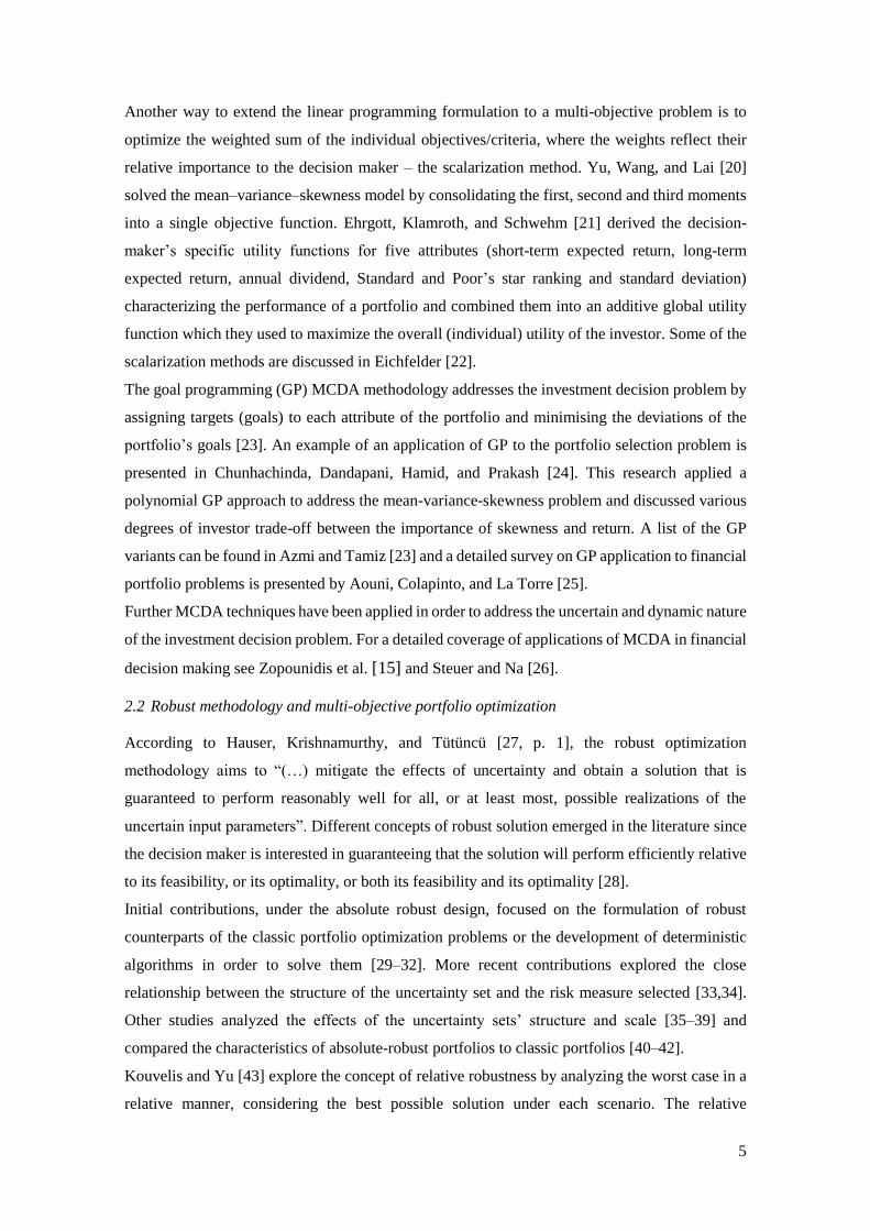
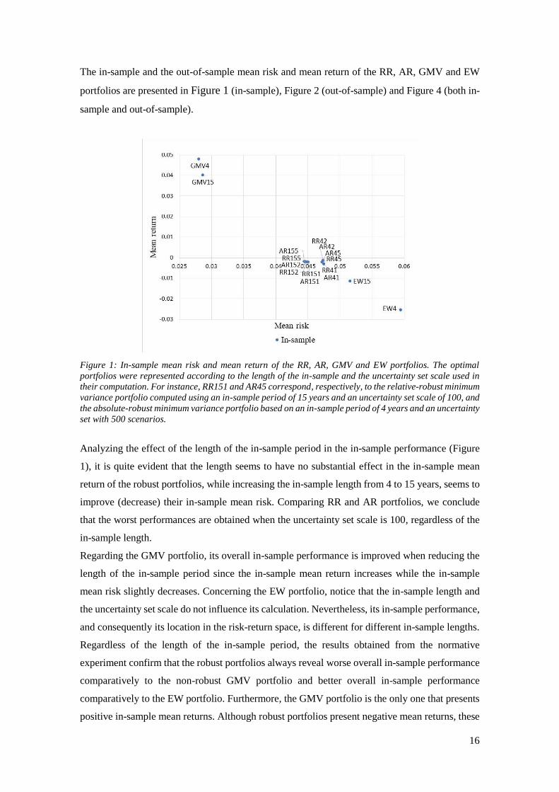
The in-sample and the out-of-sample mean risk and mean return of the RR, AR, GMV and EW
portfolios are presented in Figure 1 (in-sample), Figure 2 (out-of-sample) and Figure 4 (both in-
sample and out-of-sample).
Figure 1: In-sample mean risk and mean return of the RR, AR, GMV and EW portfolios. The optimal
portfolios were represented according to the length of the in-sample and the uncertainty set scale used in
their computation. For instance, RR151 and AR45 correspond, respectively, to the relative-robust minimum
variance portfolio computed using an in-sample period of 15 years and an uncertainty set scale of 100, and
the absolute-robust minimum variance portfolio based on an in-sample period of 4 years and an uncertainty
set with 500 scenarios.
Analyzing the effect of the length of the in-sample period in the in-sample performance (Figure
1), it is quite evident that the length seems to have no substantial effect in the in-sample mean
return of the robust portfolios, while increasing the in-sample length from 4 to 15 years, seems to
improve (decrease) their in-sample mean risk. Comparing RR and AR portfolios, we conclude
that the worst performances are obtained when the uncertainty set scale is 100, regardless of the
in-sample length.
Regarding the GMV portfolio, its overall in-sample performance is improved when reducing the
length of the in-sample period since the in-sample mean return increases while the in-sample
mean risk slightly decreases. Concerning the EW portfolio, notice that the in-sample length and
the uncertainty set scale do not influence its calculation. Nevertheless, its in-sample performance,
and consequently its location in the risk-return space, is different for different in-sample lengths.
Regardless of the length of the in-sample period, the results obtained from the normative
experiment confirm that the robust portfolios always reveal worse overall in-sample performance
comparatively to the non-robust GMV portfolio and better overall in-sample performance
comparatively to the EW portfolio. Furthermore, the GMV portfolio is the only one that presents
positive in-sample mean returns. Although robust portfolios present negative mean returns, these
17
values are close to 0% and represent substantially smaller losses than those incurred by the EW
portfolio.
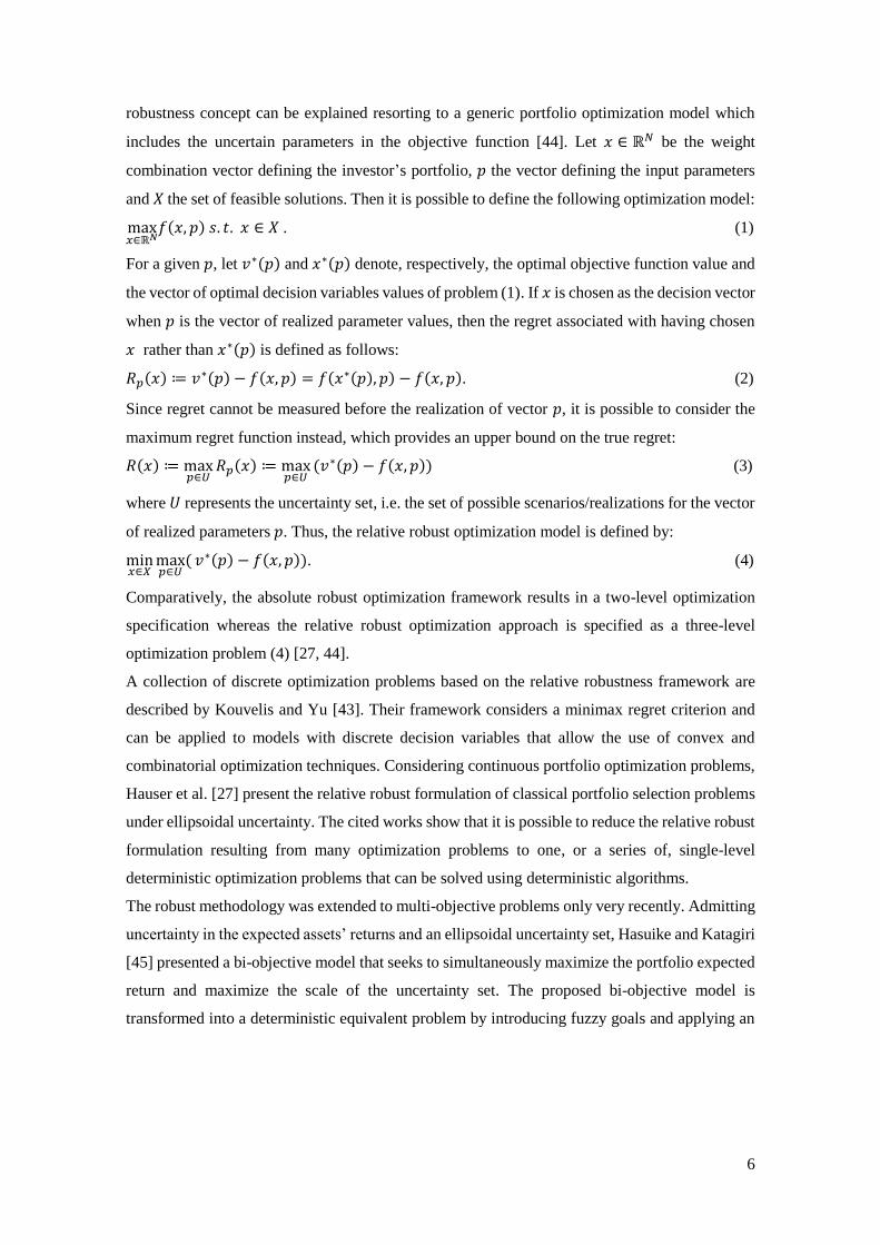
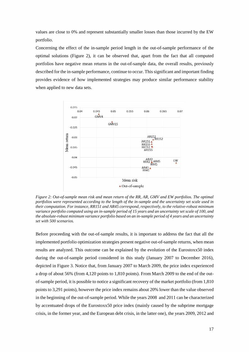
Concerning the effect of the in-sample period length in the out-of-sample performance of the
optimal solutions (Figure 2), it can be observed that, apart from the fact that all computed
portfolios have negative mean returns in the out-of-sample data, the overall results, previously
described for the in-sample performance, continue to occur. This significant and important finding
provides evidence of how implemented strategies may produce similar performance stability
when applied to new data sets.
Figure 2: Out-of-sample mean risk and mean return of the RR, AR, GMV and EW portfolios. The optimal
portfolios were represented according to the length of the in-sample and the uncertainty set scale used in
their computation. For instance, RR151 and AR45 correspond, respectively, to the relative-robust minimum
variance portfolio computed using an in-sample period of 15 years and an uncertainty set scale of 100, and
the absolute-robust minimum variance portfolio based on an in-sample period of 4 years and an uncertainty
set with 500 scenarios.
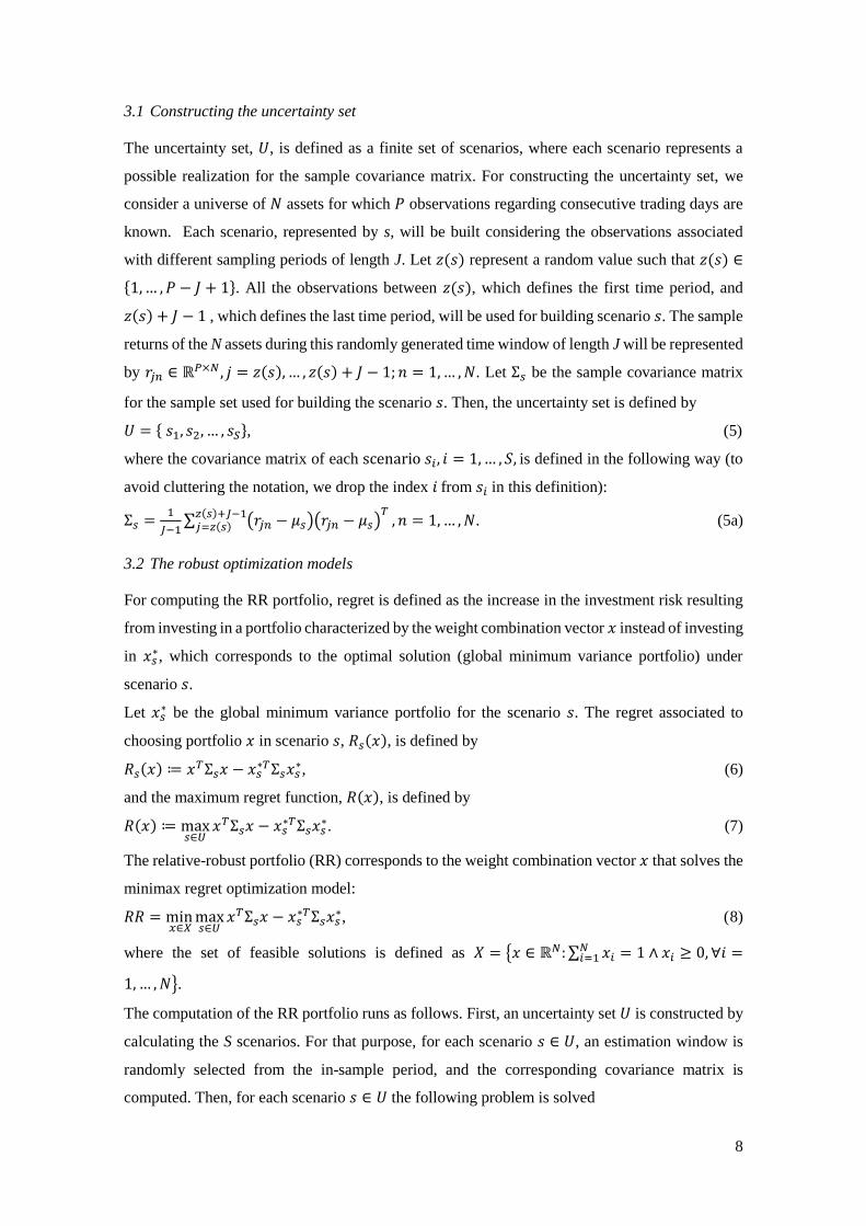
Before proceeding with the out-of-sample results, it is important to address the fact that all the
implemented portfolio optimization strategies present negative out-of-sample returns, when mean
results are analyzed. This outcome can be explained by the evolution of the Eurostoxx50 index
during the out-of-sample period considered in this study (January 2007 to December 2016),
depicted in Figure 3. Notice that, from January 2007 to March 2009, the price index experienced
a drop of about 56% (from 4,120 points to 1,810 points). From March 2009 to the end of the out-
of-sample period, it is possible to notice a significant recovery of the market portfolio (from 1,810
points to 3,291 points), however the price index remains about 20% lower than the value observed
in the beginning of the out-of-sample period. While the years 2008 and 2011 can be characterized
by accentuated drops of the Eurostoxx50 price index (mainly caused by the subprime mortgage
crisis, in the former year, and the European debt crisis, in the latter one), the years 2009, 2012 and
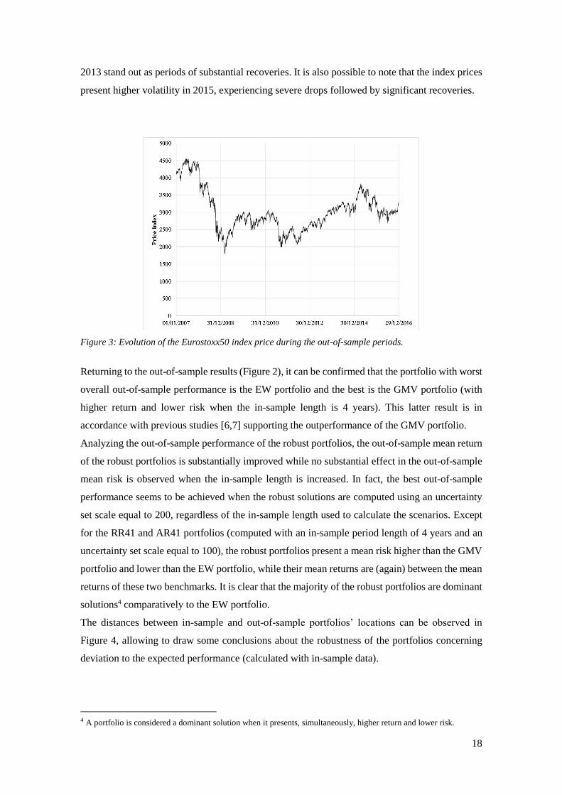
18
2013 stand out as periods of substantial recoveries. It is also possible to note that the index prices
present higher volatility in 2015, experiencing severe drops followed by significant recoveries.
Figure 3: Evolution of the Eurostoxx50 index price during the out-of-sample periods.
Returning to the out-of-sample results (Figure 2), it can be confirmed that the portfolio with worst
overall out-of-sample performance is the EW portfolio and the best is the GMV portfolio (with
higher return and lower risk when the in-sample length is 4 years). This latter result is in
accordance with previous studies [6,7] supporting the outperformance of the GMV portfolio.
Analyzing the out-of-sample performance of the robust portfolios, the out-of-sample mean return
of the robust portfolios is substantially improved while no substantial effect in the out-of-sample
mean risk is observed when the in-sample length is increased. In fact, the best out-of-sample
performance seems to be achieved when the robust solutions are computed using an uncertainty
set scale equal to 200, regardless of the in-sample length used to calculate the scenarios. Except
for the RR41 and AR41 portfolios (computed with an in-sample period length of 4 years and an
uncertainty set scale equal to 100), the robust portfolios present a mean risk higher than the GMV
portfolio and lower than the EW portfolio, while their mean returns are (again) between the mean
returns of these two benchmarks. It is clear that the majority of the robust portfolios are dominant
solutions4 comparatively to the EW portfolio.
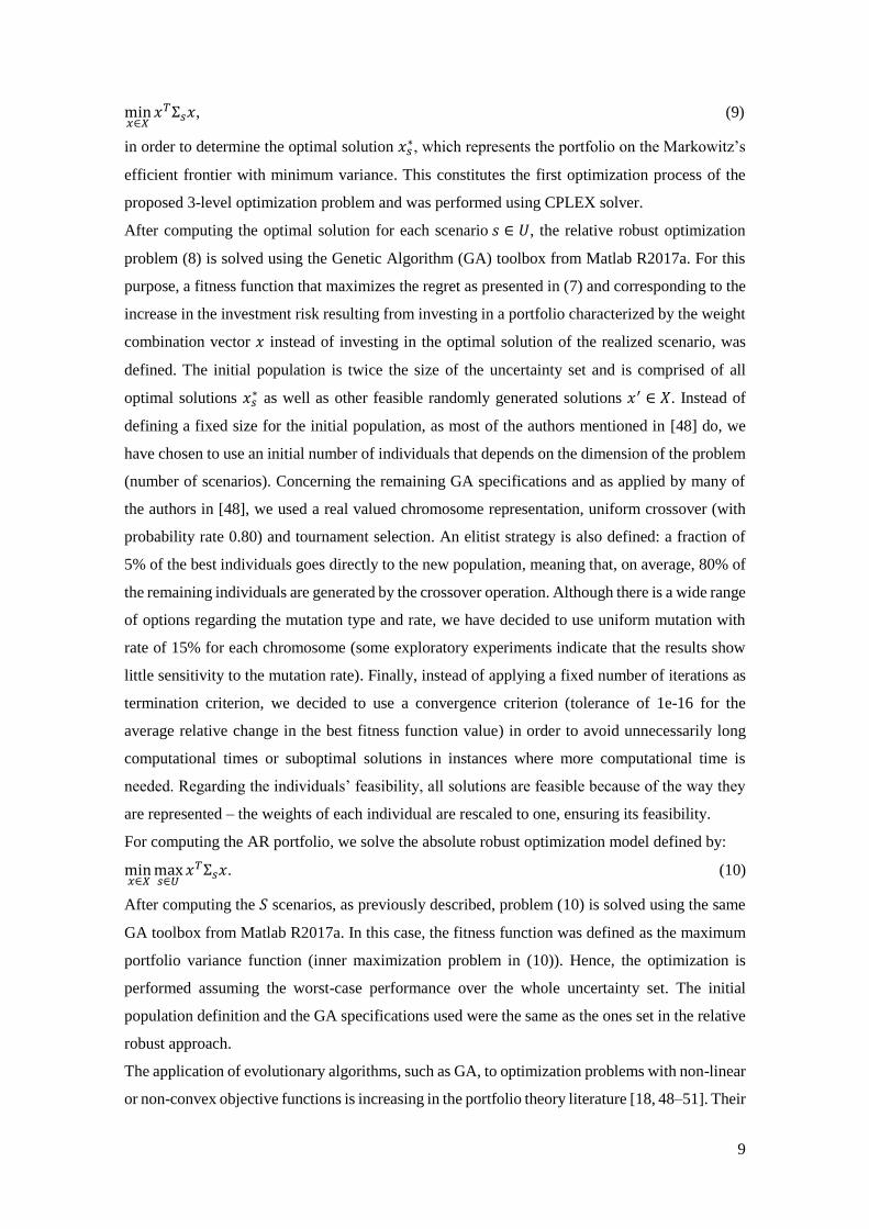
The distances between in-sample and out-of-sample portfolios’ locations can be observed in
Figure 4, allowing to draw some conclusions about the robustness of the portfolios concerning
deviation to the expected performance (calculated with in-sample data).
4 A portfolio is considered a dominant solution when it presents, simultaneously, higher return and lower risk.
19
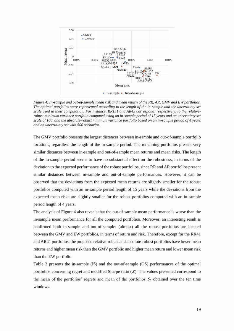
Figure 4: In-sample and out-of-sample mean risk and mean return of the RR, AR, GMV and EW portfolios.
The optimal portfolios were represented according to the length of the in-sample and the uncertainty set
scale used in their computation. For instance, RR151 and AR45 correspond, respectively, to the relative-
robust minimum variance portfolio computed using an in-sample period of 15 years and an uncertainty set
scale of 100, and the absolute-robust minimum variance portfolio based on an in-sample period of 4 years
and an uncertainty set with 500 scenarios.
The GMV portfolio presents the largest distances between in-sample and out-of-sample portfolio
locations, regardless the length of the in-sample period. The remaining portfolios present very
similar distances between in-sample and out-of-sample mean returns and mean risks. The length
of the in-sample period seems to have no substantial effect on the robustness, in terms of the
deviation to the expected performance of the robust portfolios, since RR and AR portfolios present
similar distances between in-sample and out-of-sample performances. However, it can be
observed that the deviations from the expected mean returns are slightly smaller for the robust
portfolios computed with an in-sample period length of 15 years while the deviations from the
expected mean risks are slightly smaller for the robust portfolios computed with an in-sample
period length of 4 years.
The analysis of Figure 4 also reveals that the out-of-sample mean performance is worse than the
in-sample mean performance for all the computed portfolios. Moreover, an interesting result is
confirmed both in-sample and out-of-sample: (almost) all the robust portfolios are located
between the GMV and EW portfolios, in terms of return and risk. Therefore, except for the RR41
and AR41 portfolios, the proposed relative-robust and absolute-robust portfolios have lower mean
returns and higher mean risk than the GMV portfolio and higher mean return and lower mean risk
than the EW portfolio.
Table 3 presents the in-sample (IS) and the out-of-sample (OS) performances of the optimal
portfolios concerning regret and modified Sharpe ratio (SI). The values presented correspond to
the mean of the portfolios’ regrets and mean of the portfolios SI, obtained over the ten time
windows.
20
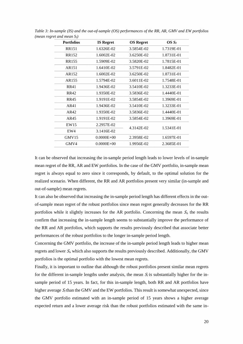
Table 3: In-sample (IS) and the out-of-sample (OS) performances of the RR, AR, GMV and EW portfolios
(mean regret and mean SI)
Portfolios IS Regret OS Regret OS SI
RR151 1.6326E-02 3.5854E-02 1.7319E-01
RR152 1.6002E-02 3.6250E-02 1.8731E-01
RR155 1.5909E-02 3.5820E-02 1.7815E-01
AR151 1.6410E-02 3.5791E-02 1.8482E-01
AR152 1.6002E-02 3.6250E-02 1.8731E-01
AR155 1.5794E-02 3.6011E-02 1.7548E-01
RR41 1.9436E-02 3.5410E-02 1.3233E-01
RR42 1.9350E-02 3.5836E-02 1.4440E-01
RR45 1.9191E-02 3.5854E-02 1.3969E-01
AR41 1.9436E-02 3.5410E-02 1.3233E-01
AR42 1.9350E-02 3.5836E-02 1.4440E-01
AR45 1.9191E-02 3.5854E-02 1.3969E-01
EW15 2.2957E-02 4.3142E-02 1.5341E-01
EW4 3.1416E-02
GMV15 0.0000E+00 2.3958E-02 1.6597E-01
GMV4 0.0000E+00 1.9956E-02 2.3685E-01
It can be observed that increasing the in-sample period length leads to lower levels of in-sample
mean regret of the RR, AR and EW portfolios. In the case of the GMV portfolio, in-sample mean
regret is always equal to zero since it corresponds, by default, to the optimal solution for the
realized scenario. When different, the RR and AR portfolios present very similar (in-sample and
out-of-sample) mean regrets.
It can also be observed that increasing the in-sample period length has different effects in the out-
of-sample mean regret of the robust portfolios since mean regret generally decreases for the RR
portfolios while it slightly increases for the AR portfolio. Concerning the mean SI, the results
confirm that increasing the in-sample length seems to substantially improve the performance of
the RR and AR portfolios, which supports the results previously described that associate better
performances of the robust portfolios to the longer in-sample period length.
Concerning the GMV portfolio, the increase of the in-sample period length leads to higher mean
regrets and lower SI, which also supports the results previously described. Additionally, the GMV
portfolios is the optimal portfolio with the lowest mean regrets.
Finally, it is important to outline that although the robust portfolios present similar mean regrets
for the different in-sample lengths under analysis, the mean SI is substantially higher for the in-
sample period of 15 years. In fact, for this in-sample length, both RR and AR portfolios have
higher average SI than the GMV and the EW portfolios. This result is somewhat unexpected, since
the GMV portfolio estimated with an in-sample period of 15 years shows a higher average
expected return and a lower average risk than the robust portfolios estimated with the same in-
21
sample period length. However, as we will see in the next sub-section, for the 1998-2013 window,
the GMV portfolio has a low out-of-sample return (close to 3%) while the robust portfolios show
high returns (between 15% and 20%). Since the out-of-sample portfolio risk measures are low in
this window, the use of a ratio between return and risk amplifies the difference in returns and ends
up leading to a higher average SI for the robust portfolios.
The analysis of the in-sample and out-of-sample performances of robust and non-robust
portfolios, for each of the 10 windows, is presented next. Since the RR and the AR portfolios,
generally present better performances for the in-sample period length corresponding to 15 years
of historical data, results are described for this particular case. The results that will be presented
in the next section generally prevail regardless of the length of the in-sample period.
4.3.2 Performance of relative-robust and non-robust portfolios
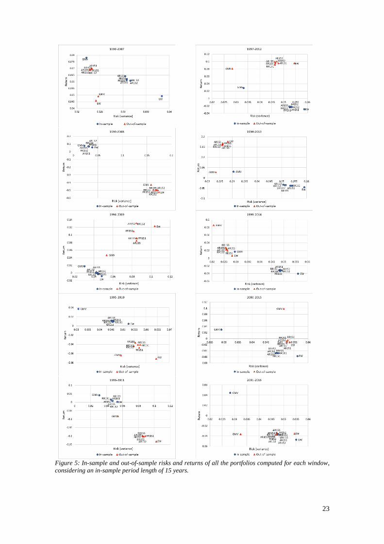
Figure 5 and Tables 4 and 5 show the performance, in each window, of the portfolios calculated
with an in-sample period length of 15 years. Starting the analysis with the results concerning the
in-sample performance of the computed portfolios, the following results were verified in all the
windows. First, the GMV portfolio is the dominant solution comparatively to all the other
portfolios under analysis. Second, the EW is the worst-performing portfolio, presenting lower
returns and higher risk than the remaining portfolios. Third, the AR and RR portfolios present
very similar performances and are always located between the GMV and the EW portfolios, in
terms of both return and risk. Regarding the location of the robust portfolios in the risk-return
space, it is also important to point out that they are always closer to the EW portfolio than to the
GMV portfolio.
Concerning the out-of-sample performance, some differences can be observed comparatively to
the in-sample results previously described. In particular, the GMV portfolio is not a dominant
solution in all the out-of-sample years under analysis. In fact, the outperformance of the GMV
portfolio is only confirmed when comparing out-of-sample portfolio risk measures, presenting
the lowest risk in all windows, except for the 1992-2007 period where the robust portfolios present
themselves as dominant solutions. The GMV portfolio underperforms, comparatively to the other
portfolios, when out-of-sample returns are compared in the (out-of-sample) years 2007, 2009,
2010, 2012 and 2013, where this portfolio presents the lowest return or is among those with the
lowest returns. Recall that 2009, 2012 and 2013 were previously described as periods where the
Eurostoxx50 index experienced significant recoveries. Additionally, and comparatively to the
other portfolios, the GMV portfolio reveals the highest return in the years 2008 and 2011, where
all the computed portfolios present negative returns. These results support previous findings
concerning the underperformance of the GMV portfolio in bull markets and its outperformance
in bear markets [56].

22
Considering the EW portfolio, the underperformance is generally confirmed both in terms of risk
and return. This portfolio always presents the highest risk with the exception of the 1992-2007
period, where it is the GMV portfolio that reveals the highest risk. Concerning out-of-sample
returns, conflicting results can be observed since the EW portfolio is among those with best
performance in some out-of-sample years (2009, 2012 and 2013) while it reveals the worst
performance in others (2007, 2008, 2010, 2011 and 2014).
Analyzing the out-of-sample performance of the robust portfolios, it can be confirmed that the
robust solutions present very similar performances, as previously suggested by the averaged
results. In fact, there is no AR or RR portfolio that systematically stands out as a dominant solution
comparatively to the other robust portfolios. Furthermore, the dominance of the robust solutions
over the EW portfolio is confirmed for the majority of the RR and AR portfolios and all the
windows under analysis, except in the out-of-sample years 2009, 2012, 2013, 2015 and 2016.
Although the robust portfolios are not dominant solutions comparatively to the EW portfolios in
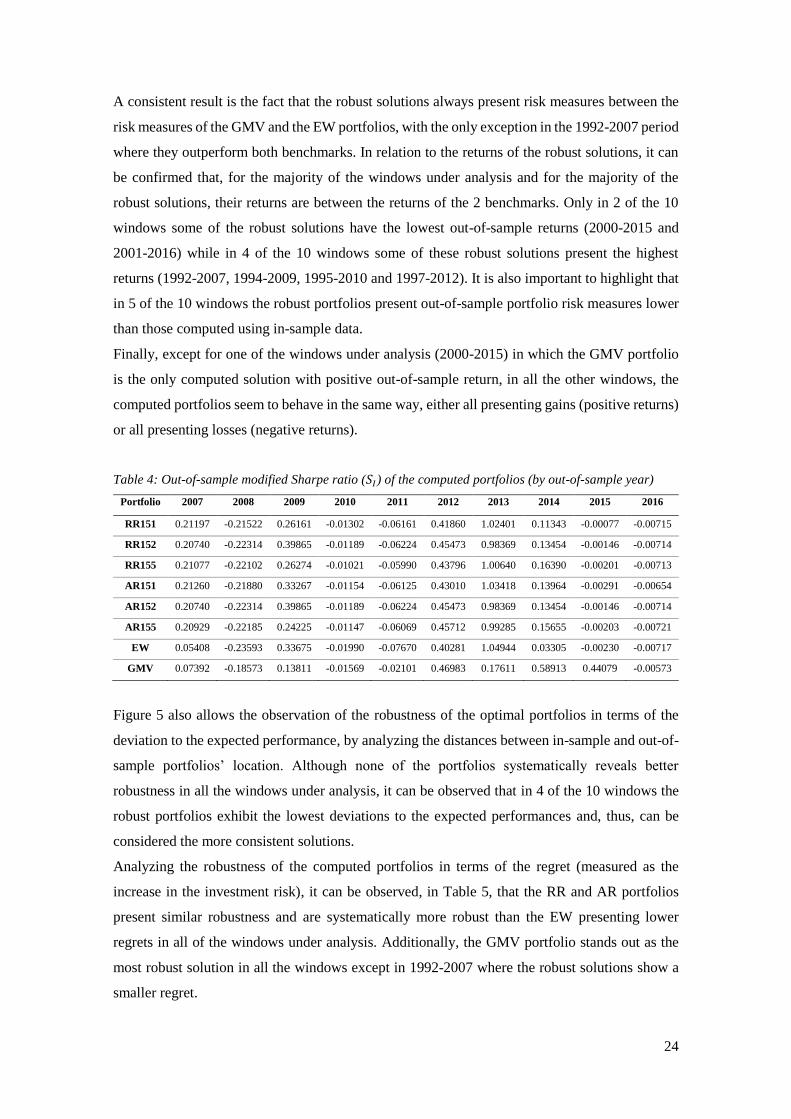
these periods, they generally outperform when the 𝑆𝐼 measure is considered (Table 4). In fact, the
robust portfolios present higher 𝑆𝐼 than the EW portfolio in all the windows under analysis with
the only exception in 2013. Comparatively to the GMV portfolio the robust portfolios do not
(generally) stand out as dominant solutions, but present higher out-of-sample returns in 5 of the
10 windows (1992-2007, 1994-2009, 1995-2010, 1997-2012 and 1998-2013); namely in periods
characterized by significant recoveries of the Eurostoxx50 index. Moreover, the majority of the
robust solutions present higher 𝑆𝐼 than the GMV portfolio in 3 of the 10 windows (1992-2007,
1994-2009, 1995-2010).
23
Figure 5: In-sample and out-of-sample risks and returns of all the portfolios computed for each window,
considering an in-sample period length of 15 years.
24
A consistent result is the fact that the robust solutions always present risk measures between the
risk measures of the GMV and the EW portfolios, with the only exception in the 1992-2007 period
where they outperform both benchmarks. In relation to the returns of the robust solutions, it can
be confirmed that, for the majority of the windows under analysis and for the majority of the
robust solutions, their returns are between the returns of the 2 benchmarks. Only in 2 of the 10
windows some of the robust solutions have the lowest out-of-sample returns (2000-2015 and
2001-2016) while in 4 of the 10 windows some of these robust solutions present the highest
returns (1992-2007, 1994-2009, 1995-2010 and 1997-2012). It is also important to highlight that
in 5 of the 10 windows the robust portfolios present out-of-sample portfolio risk measures lower
than those computed using in-sample data.
Finally, except for one of the windows under analysis (2000-2015) in which the GMV portfolio
is the only computed solution with positive out-of-sample return, in all the other windows, the
computed portfolios seem to behave in the same way, either all presenting gains (positive returns)
or all presenting losses (negative returns).
Table 4: Out-of-sample modified Sharpe ratio (𝑆𝐼) of the computed portfolios (by out-of-sample year)
Portfolio 2007 2008 2009 2010 2011 2012 2013 2014 2015 2016
RR151 0.21197 -0.21522 0.26161 -0.01302 -0.06161 0.41860 1.02401 0.11343 -0.00077 -0.00715
RR152 0.20740 -0.22314 0.39865 -0.01189 -0.06224 0.45473 0.98369 0.13454 -0.00146 -0.00714
RR155 0.21077 -0.22102 0.26274 -0.01021 -0.05990 0.43796 1.00640 0.16390 -0.00201 -0.00713
AR151 0.21260 -0.21880 0.33267 -0.01154 -0.06125 0.43010 1.03418 0.13964 -0.00291 -0.00654
AR152 0.20740 -0.22314 0.39865 -0.01189 -0.06224 0.45473 0.98369 0.13454 -0.00146 -0.00714
AR155 0.20929 -0.22185 0.24225 -0.01147 -0.06069 0.45712 0.99285 0.15655 -0.00203 -0.00721
EW 0.05408 -0.23593 0.33675 -0.01990 -0.07670 0.40281 1.04944 0.03305 -0.00230 -0.00717
GMV 0.07392 -0.18573 0.13811 -0.01569 -0.02101 0.46983 0.17611 0.58913 0.44079 -0.00573
Figure 5 also allows the observation of the robustness of the optimal portfolios in terms of the
deviation to the expected performance, by analyzing the distances between in-sample and out-of-
sample portfolios’ location. Although none of the portfolios systematically reveals better
robustness in all the windows under analysis, it can be observed that in 4 of the 10 windows the
robust portfolios exhibit the lowest deviations to the expected performances and, thus, can be
considered the more consistent solutions.
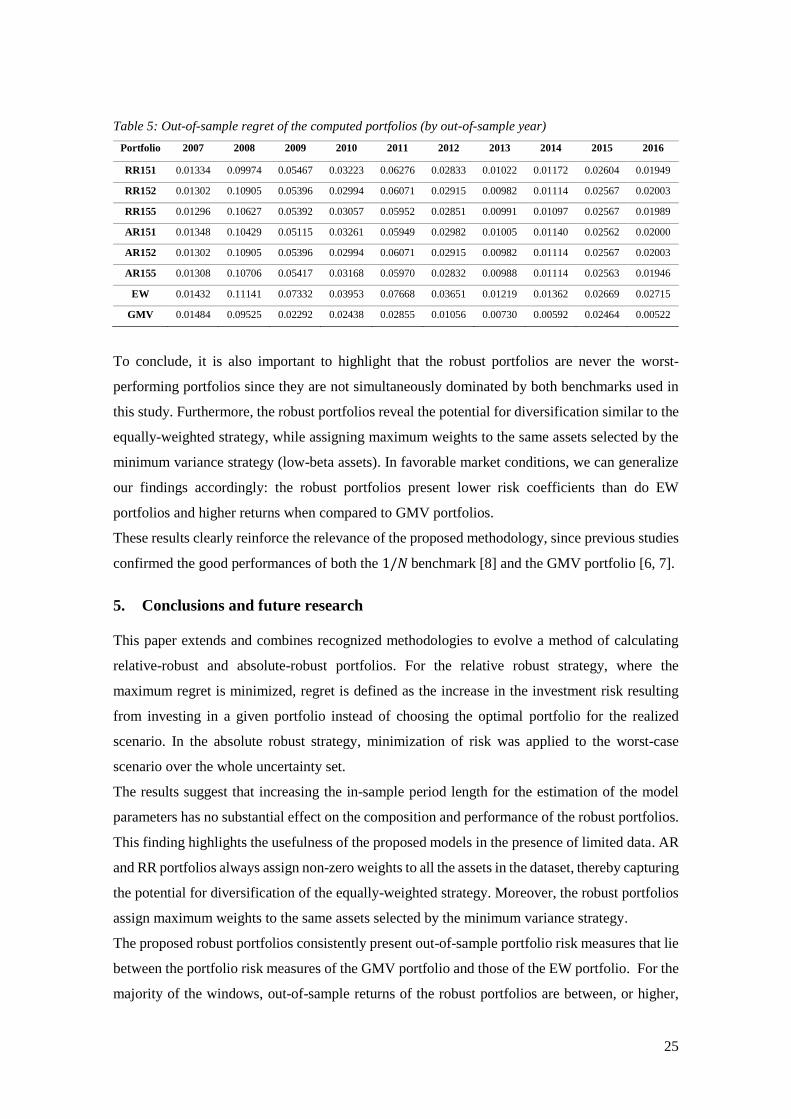
Analyzing the robustness of the computed portfolios in terms of the regret (measured as the
increase in the investment risk), it can be observed, in Table 5, that the RR and AR portfolios
present similar robustness and are systematically more robust than the EW presenting lower
regrets in all of the windows under analysis. Additionally, the GMV portfolio stands out as the
most robust solution in all the windows except in 1992-2007 where the robust solutions show a
smaller regret.
25
Table 5: Out-of-sample regret of the computed portfolios (by out-of-sample year)
Portfolio 2007 2008 2009 2010 2011 2012 2013 2014 2015 2016
RR151 0.01334 0.09974 0.05467 0.03223 0.06276 0.02833 0.01022 0.01172 0.02604 0.01949
RR152 0.01302 0.10905 0.05396 0.02994 0.06071 0.02915 0.00982 0.01114 0.02567 0.02003
RR155 0.01296 0.10627 0.05392 0.03057 0.05952 0.02851 0.00991 0.01097 0.02567 0.01989
AR151 0.01348 0.10429 0.05115 0.03261 0.05949 0.02982 0.01005 0.01140 0.02562 0.02000
AR152 0.01302 0.10905 0.05396 0.02994 0.06071 0.02915 0.00982 0.01114 0.02567 0.02003
AR155 0.01308 0.10706 0.05417 0.03168 0.05970 0.02832 0.00988 0.01114 0.02563 0.01946
EW 0.01432 0.11141 0.07332 0.03953 0.07668 0.03651 0.01219 0.01362 0.02669 0.02715
GMV 0.01484 0.09525 0.02292 0.02438 0.02855 0.01056 0.00730 0.00592 0.02464 0.00522
To conclude, it is also important to highlight that the robust portfolios are never the worst-
performing portfolios since they are not simultaneously dominated by both benchmarks used in
this study. Furthermore, the robust portfolios reveal the potential for diversification similar to the
equally-weighted strategy, while assigning maximum weights to the same assets selected by the
minimum variance strategy (low-beta assets). In favorable market conditions, we can generalize
our findings accordingly: the robust portfolios present lower risk coefficients than do EW
portfolios and higher returns when compared to GMV portfolios.
These results clearly reinforce the relevance of the proposed methodology, since previous studies
confirmed the good performances of both the 1/𝑁 benchmark [8] and the GMV portfolio [6, 7].
5. Conclusions and future research
This paper extends and combines recognized methodologies to evolve a method of calculating
relative-robust and absolute-robust portfolios. For the relative robust strategy, where the
maximum regret is minimized, regret is defined as the increase in the investment risk resulting
from investing in a given portfolio instead of choosing the optimal portfolio for the realized
scenario. In the absolute robust strategy, minimization of risk was applied to the worst-case
scenario over the whole uncertainty set.
The results suggest that increasing the in-sample period length for the estimation of the model
parameters has no substantial effect on the composition and performance of the robust portfolios.
This finding highlights the usefulness of the proposed models in the presence of limited data. AR
and RR portfolios always assign non-zero weights to all the assets in the dataset, thereby capturing
the potential for diversification of the equally-weighted strategy. Moreover, the robust portfolios
assign maximum weights to the same assets selected by the minimum variance strategy.
The proposed robust portfolios consistently present out-of-sample portfolio risk measures that lie
between the portfolio risk measures of the GMV portfolio and those of the EW portfolio. For the
majority of the windows, out-of-sample returns of the robust portfolios are between, or higher,
26
than the portfolio returns of the two benchmarks. Hence, two major conclusions can be drawn.
First, the consistent outperformance (in terms of return, risk or modified Sharpe ratio) of the
robust portfolios comparatively to the EW portfolio confirms the benefits of investing in the
optimal portfolio instead of simply allocating the investor’s wealth equally among the assets.
Second, in the presence of favorable market conditions, where the GMV portfolio performs
poorly, the robust portfolios exhibit substantially higher returns. These conclusions support the
ability of the robust strategies to optimize the first and second moments of portfolio returns.
Additionally, the empirical results provide evidence that when the distribution of the variances of
the optimal portfolios associated with the scenarios belonging to the uncertainty set is less
dispersed, the relative robust and absolute robust models may often yield identical solutions. Since
the probability of less dispersed values is higher for shorter in-sample period lengths, this is an
important outcome to take into consideration in the presence of limited data. Similar behaviours
were also observed among the robust solutions and the non-robust solutions when losses (negative
returns) versus gains (positive returns) are compared. This finding, together with the outcomes
regarding the robustness of the proposed portfolios, both in terms of increase in the investment
risk (regret) and deviations to their expected performances, suggests that the proposed
methodologies are as consistent as the benchmarks used for comparing portfolios’ out-of-sample
performances which, in our opinion, validates the proposed methodologies.
Upon review, to the decision-maker the overall results add value to the portfolio selection process
by tackling the weakness of optimization methodologies abstracted in the literature. Overall, the
results presented in this research reinforce the relevance of robust optimization within the field of
portfolio selection under uncertainty.
Future research will include the application of the proposed methodology to different datasets and
the comparison of our robust strategies to other robust formulations of the minimum variance
model that are present in the literature. An interesting comparison would be to replicate all the
minimum variance portfolios described in Maillet, Tokpavi, and Vaucher [57] and scrutinize the
characteristics as well as the performance of all robust minimum variance solutions.
Acknowledgements: This study has been funded by national funds, through FCT, Portuguese
Science Foundation, under project UID/Multi/00308/2019.
Conflict of Interest: The authors declare that they have no conflict of interest.
References
[1] H. Markowitz, Portfolio Selection: Efficient Diversification of Investments. New York:
John Wiley & Sons, 1959.
[2] H. Markowitz, “Portfolio Selection,” The Journal of Finance, vol. 7, no. 1, pp. 77–91,
Mar. 1952.
27
[3] M. J. Best and R. R. Grauer, “On the sensitivity of mean-variance-efficient portfolios to
changes in asset means: some analytical and computational results.,” Review of Financial
Studies, vol. 4, no. 2, p. 315, Jun. 1991.
[4] M. J. Best and R. R. Grauer, “Sensitivity analysis for mean-variance portfolio problems,”
Management Science, vol. 37, no. 8, pp. 980–989, Aug. 1991.
[5] V. K. Chopra and W. T. Ziemba, “The effect of errors in means, variances, and covariances
on optimal portfolio choice,” Journal of Portfolio Management, vol. 19, no. 2, pp. 6–11,
1993.
[6] R. Jagannathan and T. Ma, “Risk Reduction in Large Portfolios: Why Imposing the Wrong
Constraints Helps,” The Journal of Finance, vol. 58, no. 4, pp. 1651–1684, Aug. 2003.
[7] L. K. C. Chan, J. Karceski, and J. Lakonishok, “On portfolio optimization: forecasting
covariances and choosing the risk model.,” Review of Financial Studies, vol. 12, no. 5, pp.
937–974, 1999.
[8] V. DeMiguel, L. Garlappi, and R. Uppal, “Optimal Versus Naive Diversification: How
Inefficient is the 1/N Portfolio Strategy?,” Review of Financial Studies, vol. 22, no. 5, pp.
1915–1953, May 2009.
[9] E. D. Supandi and D. Rosadi, “An Empirical Comparison between Robust Estimation and
Robust Optimization to Mean-Variance Portfolio,” Journal of Modern Applied Statistical
Methods, vol. 16, no. 1, p. 32, 2017.
[10] F. J. Fabozzi, P. N. Kolm, D. Pachamanova, and S. M. Focardi, Robust portfolio
optimization and management. John Wiley & Sons, 2007.
[11] R. E. Steuer, Y. Qi, and M. Hirschberger, “Portfolio selection in the presence of multiple
criteria,” in Handbook of financial engineering, Springer, 2008, pp. 3–24.
[12] P. N. Kolm, R. Tütüncü, and F. J. Fabozzi, “60 Years of portfolio optimization: Practical
challenges and current trends,” European Journal of Operational Research, vol. 234, no.
2, pp. 356–371, 2014.
[13] C. Bana e Costa and J. Soares, Multicriteria approaches for portfolio selection: an
overview, vol. 4. 2001.
[14] C. Zopounidis and M. Doumpos, “Multi-criteria decision aid in financial decision making:
methodologies and literature review,” Journal of Multi-Criteria Decision Analysis, vol.
11, no. 4–5, pp. 167–186, 2002.
[15] C. Zopounidis, E. Galariotis, M. Doumpos, S. Sarri, and K. Andriosopoulos, “Multiple
criteria decision aiding for finance: An updated bibliographic survey,” European Journal
of Operational Research, vol. 247, no. 2, pp. 339–348, 2015.
[16] T.-J. Chang, N. Meade, J. E. Beasley, and Y. M. Sharaiha, “Heuristics for cardinality
constrained portfolio optimisation,” Computers & Operations Research, vol. 27, no. 13,
pp. 1271–1302, 2000.
[17] H. R. Golmakani and M. Fazel, “Constrained portfolio selection using particle swarm
optimization,” Expert Systems with Applications, vol. 38, no. 7, pp. 8327–8335, 2011.
[18] H. Soleimani, H. R. Golmakani, and M. H. Salimi, “Markowitz-based portfolio selection
with minimum transaction lots, cardinality constraints and regarding sector capitalization
using genetic algorithm,” Expert Systems with Applications, vol. 36, no. 3, Part 1, pp.
5058–5063, 2009.
[19] J. Spronk and W. Hallerbach, “Financial modelling: Where to go? With an illustration for
portfolio management,” European Journal of Operational Research, vol. 99, no. 1, pp.
113–125, 1997.
[20] L. Yu, S. Wang, and K. K. Lai, “Neural network-based mean–variance–skewness model
for portfolio selection,” Computers & Operations Research, vol. 35, no. 1, pp. 34–46,
2008.
[21] M. Ehrgott, K. Klamroth, and C. Schwehm, “An MCDM approach to portfolio
optimization,” European Journal of Operational Research, vol. 155, no. 3, pp. 752–770,
2004.
[22] G. Eichfelder, Adaptive Scalarization Methods in Multiobjective Optimization. Springer
Berlin Heidelberg, 2008.
[23] R. Azmi and M. Tamiz, “A review of goal programming for portfolio selection,” in New
28
developments in multiple objective and goal programming, Springer, 2010, pp. 15–33.
[24] P. Chunhachinda, K. Dandapani, S. Hamid, and A. J. Prakash, “Portfolio selection and
skewness: Evidence from international stock markets,” Journal of Banking & Finance,
vol. 21, no. 2, pp. 143–167, 1997.
[25] B. Aouni, C. Colapinto, and D. La Torre, “Financial portfolio management through the
goal programming model: Current state-of-the-art,” European Journal of Operational
Research, vol. 234, no. 2, pp. 536–545, 2014.
[26] R. E. Steuer and P. Na, “Multiple criteria decision making combined with finance: A
categorized bibliographic study,” European Journal of Operational Research, vol. 150,
no. 3, pp. 496–515, 2003.
[27] R. Hauser, V. Krishnamurthy, and R. Tütüncü, “Relative robust portfolio optimization,”
arXiv preprint arXiv:1305.0144, 2013.
[28] V. Gabrel, C. Murat, and A. Thiele, “Recent advances in robust optimization: An
overview,” European Journal of Operational Research, vol. 235, no. 3, pp. 471–483, Jun.
2014.
[29] L. El Ghaoui and H. Lebret, “Robust Solutions to Least-Squares Problems with Uncertain
Data,” SIAM Journal on Matrix Analysis and Applications, vol. 18, no. 4, pp. 1035–1064,
Oct. 1997.
[30] A. Ben-Tal and A. Nemirovski, “Robust Convex Optimization,” Mathematics of
Operations Research, vol. 23, no. 4, pp. 769–805, Nov. 1998.
[31] D. Goldfarb and G. Iyengar, “Robust portfolio selection problems,” Mathematics of
Operations Research, vol. 28, no. 1, pp. 1–38, 2003.
[32] B. V Halldórsson and R. H. Tütüncü, “An Interior-Point Method for a Class of Saddle-
Point Problems,” Journal of Optimization Theory and Applications, vol. 116, no. 3, pp.
559–590, 2003.
[33] K. Natarajan, D. Pachamanova, and M. Sim, “Constructing risk measures from uncertainty
sets,” Operations Research, vol. 57, no. 5, pp. 1129–1141, 2009.
[34] D. Bertsimas and D. B. Brown, “Constructing uncertainty sets for robust linear
optimization,” Operations Research, vol. 57, no. 6, pp. 1483–1495, 2009.
[35] Z. Lu, “A new cone programming approach for robust portfolio selection,” Optimization
Methods & Software, vol. 26, no. 1, pp. 89–104, 2006.
[36] Z. Lu, “A computational study on robust portfolio selection based on a joint ellipsoidal
uncertainty set,” Mathematical Programming, vol. 126, no. 1, pp. 193–201, 2011.
[37] B. Roy, “Robustness in operational research and decision aiding: A multi-faceted issue,”
European Journal of Operational Research, vol. 200, no. 3, pp. 629–638, 2010.
[38] C. Gregory, K. Darby-Dowman, and G. Mitra, “Robust optimization and portfolio
selection: The cost of robustness,” European Journal of Operational Research, vol. 212,
no. 2, pp. 417–428, Jul. 2011.
[39] R. Kaläı, C. Lamboray, and D. Vanderpooten, “Lexicographic α-robustness: An
alternative to min–max criteria,” European Journal of Operational Research, vol. 220, no.
3, pp. 722–728, Aug. 2012.
[40] J. H. Kim, W. C. Kim, and F. J. Fabozzi, “Composition of robust equity portfolios,”
Finance Research Letters, vol. 10, no. 2, pp. 72–81, Jun. 2013.
[41] W. C. Kim, J. H. Kim, S. H. Ahn, and F. J. Fabozzi, “What do robust equity portfolio
models really do?,” Annals of Operations Research, vol. 205, no. 1, pp. 141–168, 2013.
[42] W. C. Kim, J. H. Kim, and F. J. Fabozzi, “Deciphering robust portfolios,” Journal of
Banking & Finance, vol. 45, pp. 1–8, Aug. 2014.
[43] P. Kouvelis and G. Yu, “Robust Discrete Optimization: Past Successes and Future
Challenges,” in Robust Discrete Optimization and Its Applications, Boston, MA: Springer
US, 1997, pp. 333–356.
[44] G. Cornuejols and R. Tütüncü, Optimization Methods in Finance. Cambridge: Cambridge
University Press, 2006.
[45] T. Hasuike and H. Katagiri, “Robust-based interactive portfolio selection problems with
an uncertainty set of returns,” Fuzzy Optimization and Decision Making, vol. 12, no. 3,
pp. 263–288, 2013.

29
[46] J. Fliege and R. Werner, “Robust multiobjective optimization & applications in
portfolio optimization,” European Journal of Operational Research, vol. 234, no. 2, pp.
422–433, Apr. 2014.
[47] P. Xidonas, G. Mavrotas, C. Hassapis, and C. Zopounidis, “Robust multiobjective
portfolio optimization: A minimax regret approach,” European Journal of Operational
Research, vol. 262, no. 1, pp. 299–305, 2017.
[48] C. B. Kalayci, O. Ertenlice, H. Akyer, and H. Aygoren, “A review on the current
applications of genetic algorithms in mean-variance portfolio optimization,” Pamukkale
University Journal of Engineering Sciences, vol. 23, no. 4, pp. 470–476, 2017.
[49] F. Streichert, H. Ulmer, and A. Zell, “Evolutionary algorithms and the cardinality
constrained portfolio optimization problem,” in Operations Research Proceedings 2003.
Operations Research Proceedings (GOR (Gesellschaft für Operations Research e.V.)), vol
2003., 2004, pp. 253–260.
[50] T.-J. Chang, S.-C. Yang, and K.-J. Chang, “Portfolio optimization problems in different
risk measures using genetic algorithm,” Expert Systems with Applications, vol. 36, no. 7,
pp. 10529–10537, 2009.
[51] H. Zhu, Y. Wang, K. Wang, and Y. Chen, “Particle Swarm Optimization (PSO) for the
constrained portfolio optimization problem,” Expert Systems with Applications, vol. 38,
no. 8, pp. 10161–10169, 2011.
[52] D. W. Blackburn and N. Cakici, “Overreaction and the cross-section of returns:
International evidence,” Journal of Empirical Finance, vol. 42, pp. 1–14, 2017.
[53] N. Jegadeesh and S. Titman, “Returns to buying winners and selling losers: Implications
for stock market efficiency,” The Journal of finance, vol. 48, no. 1, pp. 65–91, 1993.
[54] C. L. Israelsen, “A refinement to the Sharpe ratio and information ratio.,” Journal of Asset
Management, vol. 5, no. 6, pp. 423–427, Apr. 2005.
[55] P. Cogneau and G. Hübner, “The 101 Ways to Measure Portfolio Performance,” 2009.
[Online]. Available: http://dx.doi.org/10.2139/ssrn.1326076.
[56] T.-M. Chow, J. C. Hsu, L.-L. Kuo, and F. Li, “A study of low-volatility portfolio
construction methods,” Journal of Portfolio Management, vol. 40, no. 4, pp. 89–105,
2014.
[57] B. Maillet, S. Tokpavi, and B. Vaucher, “Global minimum variance portfolio optimisation
under some model risk: A robust regression-based approach,” European Journal of
Operational Research, vol. 244, no. 1, pp. 289–299, 2015.
[58] L. Duan and P. Stahlecker, “A portfolio selection model using fuzzy returns,” Fuzzy
Optimization and Decision Making, vol. 10, no. 2, pp. 167–191, 2011.
[59] K. Kato and M. Sakawa, “An interactive fuzzy satisficing method based on variance
minimization under expectation constraints for multiobjective stochastic linear
programming problems,” Soft Computing, vol. 15, no. 1, pp. 131–138, 2011.


