Global Minima Analysis of Lee and Seungâs NMF Algorithms

Neural Process LettDOI 10.1007/s11063-012-9261-x

Global Minima Analysis of Lee and Seung’s NMFAlgorithms

Shangming Yang · Mao Ye

© Springer Science+Business Media New York 2012

Abstract Lee and Seung proposed nonnegative matrix factorization (NMF) algorithmsto decompose patterns and images for structure retrieving. The NMF algorithms have beenapplied to various optimization problems. However, it is difficult to prove the convergenceof this class of learning algorithms. This paper presents the global minima analysis of theNMF algorithms. In the analysis, invariant set is constructed so that the non-divergence ofthe algorithms can be guaranteed in the set. Using the features of linear equation systemsand their solutions, the fixed points and convergence properties of the update algorithms arediscussed in detail. The analysis shows that, although the cost function is not convex in bothA and X together, it is possible to obtain the global minima from the particular learningalgorithms. For different initializations, simulations are presented to confirm the analysisresults.

Keywords BSS · Structure retrieving · Global minima analysis ·Non-negative matrix factorization · NMF · KL divergence

1 Introduction

Non-negative matrix factorization (NMF) algorithms are designed to extract alternative struc-tures inherent in the data we observed [1–5]. This method has been applied to different fieldsfrom engineering to neuroscience. In [2,3], authors discussed NMF for blind source sep-aration(BSS). Without the assumption of independence, they achieved estimations of theoriginal sources from the mixtures by NMF methods. Plumbley and Oja [6,7] proposed analgorithm to obtain a nonnegative matrix factorization of known mixtures, which is a special

S. Yang (B) ·M. YeSchool of Computer Science and Engineering, University of Electronic Science and Technology of China,Chengdu 610054, People’s Republic of Chinae-mail: [email protected]

M. Yee-mail: [email protected]

123

S. Yang, M. Ye

case of the non-linear PCA algorithm. Their research showed that this method could findnonnegative well-grounded independent sources. NMF as a method to decompose patternsand images was introduced by Lee and Seung, and they also proved that in the updates thedivergence DK L(Y||AX) was non-increasing [8]. This method is called multiplicative learn-ing update algorithm. Convergence analysis is very important for the application of NMFalgorithms. Studies showed that NMF update algorithms may converge to a saddle point[9,10]. Lin [11] discussed the difficulty of proving the multiplicative update convergence,and he proposed some slight modifications of existing updates and proved their convergence.Lee and Seung’s NMF method is popular due to its simplicity. For this class of algorithms,stationarity is a necessary condition in the determination of local minima. Gonzales andZhang’s [12] research showed that in some conditions, Lee and Seung’s algorithms mayfail to approach a stationary point. By constructing an alternating minimization algorithm,Finesso and Spreij indirectly analyzed the convergence of the NMF algorithms [13]. Recently,Badeau proved the exponential or the asymptotic stability of the local minima of the NMFalgorithms under some mild conditions [14]. Badeau’s research focused on the local con-vergence of a class of general NMF algorithms, but the existence of global minima was notstudied. In [15], the convergence of the NMF based BSS algorithms was analyzed, whichshowed that the local convergence can be guaranteed in some predefined areas. However,since all elements in A and X are variables in the updates, the predefined areas are changeableduring the learning updates. It will be very difficult to test these conditions in the applications.In [16], the local convergence of the α-divergence NMF algorithms for different values of α

was discussed. The analysis showed that this class of NMF algorithms can converge to theirlocal minima. In this paper, an invariant set is constructed to show the non-divergence ofthe learning algorithms. Based on the invariant set, the local convergence of the NMF algo-rithms is discussed. The analysis will show that the NMF update algorithms can convergeto constants in the domain of the learning algorithms and the most important result is thatthe global minimum of the cost function can be obtained in the learning. The NMF decom-poses the data matrix Y = [y(1), y(2), . . . , y(N )] ∈ Rm×N to two matrices A ∈ Rm×n andX = [x(1), x(2), . . . , x(N )] ∈ Rn×N having only non-negative elements in each matrix. Weconsider decompositions which are approximative in a model as

Y ≈ AX (1)

or a vector form as

y ≈ Ax. (2)

For the convergence analysis, a detailed scalar form of the decomposition in the followingis very useful:

yi (k) ≈n∑

j=1

ai j x j (k), i = 1, . . . , m, k = 1, 2, . . . , N , (3)

where y(k) = [y1(k), …, ym(k)]T is a vector of the observations at the discrete time instantsk and x(k) = [x1(k), . . . , xn(k)]T is a vector of components at the same time instant. Usu-ally, A is called the basis of the observation matrix Y and each column of X is called anencoding. From the view of blind source separation, the objective of the NMF algorithmsis to estimate a basis matrix A and sources X subject to non-negativity constraints, andthe non-negative sources X will be the original sources we expect to find out. Similar tothe definitions in Cichocki’s research, we will use the following notations in the analysis:

123

Global Minima Analysis of Lee and Seung’s NMF Algorithms

x j (k) = x jk, yi (k) = yik, zik = [AX]ik is the ik-element of the matrix AX and ai j is thei j th element of the matrix A.

2 Related Work

NMF is an important approach to decompose data into nonnegative factors. Up to now, a lotof NMF algorithms have been proposed to satisfy to the necessity of intelligent recognitionand detection. For these algorithms, convergence analysis plays an important role for theirapplications. In this section, we will introduce the basic ideas of these algorithms and theirconvergence properties.

By extending sparsity and smoothness constraints to NMF learning rules and their corre-sponding loss functions, NMF algorithms can be used for blind source separation (BSS). Acommon approach is adding suitable regularization terms to the cost functions. For exam-ple, Cichocki et al. [2] proposed the following generalized regularized Kullback–Leiblerdivergence to generate NMF based BSS algorithms:

DK L(Y||AX) =∑

ik

(log

yik

[AX]ik+ yik − [AX]ik

)+ αX J (X)+ αA J (A)

where the small positive terms αX > 0 and αA > 0 are used to enforce sparseness of thedecomposition, and terms JX (X) and JA(A) are introduced to add application-dependentcharacteristics to the separation results. However, the global convergence of this class ofalgorithms is still an open issue.

Most NMF algorithms have multiple fixed points, which can only obtain local minimumpoints in the learning. To solve this problem, Zhou et al. [17] proposed an incrementalnon-negative matrix factorization (INMF) by imposing a volume constraint to achieve theuniqueness:

minA∈C,X≥0

Dt+1 �1

2||Y− AX||2F + μ ln |detA|.

By minimizing the determinant of A, this algorithm can obtain the unique data decompo-sition, and at the same time, the parameter μ can balance the approximation error of NMFalgorithms.

Manifold learning NMF algorithms was proposed by adding geometric information to thecost function [18]:

DK L(Y||AX) =∑

ik

(log

yik


)

+λ

2

∑

j,l,k

(x jk log

xi j

xlk+ xlk log

xlk

x jk

)w jl ,

where the regularization parameter λ ≥ 0 controls the smoothness of the new representation,and w jl is the weight of two connected nodes of a graph. For this class of NMF algorithms,since the geometric structures of graph are considered, it will better extract information forimage recognition and detection.

123

S. Yang, M. Ye

Convergence analysis is an interesting topic for NMF algorithms. Assume that f (A, X)

is the cost function; A and X are the separation results. Lee and Seung proved that in thelearning

f (At , Xt+1) ≤ f (At , Xt ) and f (At+1, Xt+1) ≤ f (At , Xt+1),

which indicates that this function is non-increasing under its corresponding update rules [8].Studies show that such properties cannot guarantee the convergence to a stationary point

of the algorithm. Lin [11] proposed a new NMF method by modifying the step size of thelearning algorithms to:

x jk

[AT AX] jk + δ

where

x jk ≡{

x jk if ∇X f (A, X) jk ≥ 0,

max(x jk, σ ) if ∇X f (A, X) jk < 0,

where σ and δ are pre-defined positive numbers. ai j can be defined similarly. Then theconvergence of the learning algorithms can be guaranteed.

Recently, based on the Lyapunov indirect method, Badeau proved the local convergenceof the Lee and Seung’s NMF algorithms [14]. The general idea of this proof is as follows:

Assume that x (we can consider it a vector consisting of all elements in matrices A andX) is a local minimum of the cost function f . Denote

P(x) = D(x)∇2 f (x)D(x), η = 2

‖P(x)‖2

where D(x) = diag(x/p(x))12 ,∇ f (x) = p(x)−m(x), p(x) and m(x) are two non-negative

functions. Using Lyapunov indirect method, the following results can be proved:If η > 1 and matrix [P(x)]+ (if an element in P(x) is negative, then set it zero) non-singu-

lar, then x is an exponentially stable fixed point; if η < 1, x is an unstable (non-convergence)fixed point; if η = 1, the stability of fixed point x can not be determined. The results showthat we need to test the conditions in the application so that the local convergence of thealgorithms can be guaranteed.

NMF have been applied to different area. One of the most important fields is for face rec-ognition. For this class of algorithms, the features of graph were added to the cost functionso that their corresponding learning algorithms could be more effective [17–20]. Similar tothe Lee and Seung’s NMF, the convergence of the algorithms was analyzed by proving thenon-increasing of cost function. Thus, most of these algorithms need further convergenceanalysis so that they can be applied efficiently.

3 Preliminaries

Imposing nonnegativity constraint is useful for matrix decomposition of learning a parts rep-resentation of the observations. To obtain learning algorithms for this type of decomposition,the regularized general KL divergence was used as the cost function [3]:

123


DK L (Y||AX) =∑

ik

(log

yik


)

s.t. ai j ≥ 0, x jk ≥ 0, (4)

||a j ||1 =m∑

i=1

ai j = 1, ∀i, j, k ∈ N ,

From the cost function in (4), Lee and Seung proposed learning rules as follows:

x jk ← x jk

∑mi=1 ai j (yik/[AX]ik)∑m

q=1 aq j, (5)

ai j ← ai j

∑Nk=1 x jk(yik/[AX]ik)∑N

p=1 x jp, (6)

where ai j is normalized in each step as ai j = ai j/∑

p apj .According to the definitions of A and X, the following matrix operation expression holds:

[AX]ik =n∑

p=1

aipx pk = ai j x jk +n∑

p=1, �= j

aipx pk, (7)

which will be used in the further analysis.To prove the non-divergence of the NMF learning update algorithms (5) and (6), we start

from the following definitions:

Definition 1 For the update algorithm (5), a point x jk ∈ R is called a fixed point of theupdate iterations, if and only if

x jk = x jk


q=1 aq j. (8)

Definition 2 For the update algorithm (6), a point ai j ∈ R is called a fixed point of theupdate iterations, if and only if

ai j = ai j


p=1 x jp. (9)

Denote

f (x jk) = x jk − x jk


q=1 aq j, (10)

g(ai j ) = ai j − ai j


p=1 x jp, (11)

where yik are elements of observation samples, a jk ∈ [0, 1], x jk ∈ [0,+∞). The point x jk

satisfying Eq. (8) or the point ai j satisfying Eq. (9) is also called an equilibrium point of thecorresponding update algorithm. The existence of fixed points of update algorithms (5) and(6) is just the existence of the solutions of Eqs. (8) and (9).

123

S. Yang, M. Ye

From (7), at the fixed point, Eq. (8) can be rewritten as

x jk = x jk

∑mi=1 ai j (yik/

∑np=1 aipx pk)∑m

q=1 aq j

= x jk

∑mi=1 ai j (yik/(ai j x jk +∑n

p=1, �= j aipx pk))∑mq=1 aq j

= x jk∑mq=1 aq j

m∑

i=1

ai j yik

ai j x jk +∑np=1, �= j aipx pk

= x jk

m∑

i=1

ai j yik∑mq=1 aq j

ai j x jk +∑np=1, �= j aipx pk

. (12)

Assuming

ci = ai j yik∑mq=1 aq j

, bi = ai j , ai =n∑

p=1, �= j

aipx pk, (13)

Eq. (8) can be simplified to

x = xm∑

i=1

ci

ai + bi x, (14)

where x represents x jk , is the only variable in a single update computing and for all i, ai andbi cannot be zeros at the same time. We must understand that in the learning, x, ai , and bi

are all variables. In any update step, the only constant is yik .For the update algorithm of ai j , we have similar results as follows:The term

∑Nk=1 x jk(yik/[AX]ik) in Eq. (9) can be written as

N∑

k=1

x jk(yik/[AX]ik) = x j1(yi1/[AX]i1)+ x j2(yi2/[AX]i2)+ · · · + x j N (yi N /[AX]i N )

= x j1

⎛

⎝yi1

/ n∑

p=1

aipx p1

⎞

⎠

+x j2

⎛

⎝yi2

/ n∑

p=1

aipx p2

⎞

⎠+ . . .+ x j N

⎛

⎝yi N

/ n∑

p=1

aipx pN

⎞

⎠ .

(15)

Denote

ck = x jk yik∑Np=1 x jp

, bk = x jk, ak =n∑

p=1,p �= j

aipx pk, (16)

Equation (9) can be simply written as

a = aN∑

k=1

ck

ak + bka, (17)

123


where a represents ai j , is the only variable for a single update step of ai j . Expression (17)can be used to study the structures of the fixed points.

For the update of ai j , the only difference is the normalization of ai j in each update step,but this does not change the existence of fixed points. Later in the invariant set analysis inSect. 4, we will see the necessity of normalization. In the fixed point analysis of ai j , weassume that X is temporarily considered as fixed matrix, which implies for all j,

∑Np=1 x jp

are temporary constants.

4 Existence of the Invariant Set

If an update is convergent, the updated element in the sequence must be in a limited set inany step of the learning updates. This set is called an invariant set. The invariant set of theNMF algorithms is defined as follows:

Definition 3 A compact set X ⊂ R is an invariant set of the update algorithms (5) and (6)for all i, j , and k, if x jk(0), ai j (0) ∈ X , the trajectories of (5) and (6) starting from x jk(0)

and ai j (0) respectively will remain in X for all x jk(t) and ai j (t) in the updates.

For matrix Am×n, m and n are limited numbers. Since∑m

i=1 ai j = 1, for, all i, ai j willnot be all zeros, which means, there always exists i , such that bi > 0. If x jk > 0, the updatealgorithm (5) can be written as

x jk(t + 1)← x jk(t)m∑

i=1

ci

ai + bi x jk(t)=

m∑

i=1

ci

bi + aix jk (t)

.

If ∀i, ai ≥ 0, bi and ci > 0, it holds that

0 ≤ x jk(t)m∑

i=1

ci

ai + bi x jk(t)≤

m∑

i=1

ci

bi. (18)

If ∃i , such that bi = 0, then ci = 0; it holds that

ai > 0,ci

ai + bi x jk(t)= 0.

Therefore, inequality (18) always holds. From (13), considering the normalization of ai j , itfollows that

m∑

i=1

ci

bi=

m∑

i=1

ai j yik∑mq=1 aq j

ai j=

m∑

i=1

yik, (19)

where yik(i = 1, 2 . . . , m, k = 1, 2, . . . , N ) are the observed values which are all knownand will not be changed in the update.

Assuming∑m

i=1 yik < M2 for all k, x jk(t+1) in the update algorithm (5) is always upperbounded. Since x jk(0) is not included in the sequence {x jk(t+1)}, t = 0, 1, 2, . . ., assuming0 ≤ x jk(0) ≤ M1 for all j and k(M1 is a constant decided by the initializations), then wecan prove the following Theorem 1.

Denote

M = max {M1, M2} .

123

S. Yang, M. Ye

ai j will be normalized in each learning update iteration, but the initialization may not be lessthan 1. We can simply construct a limited value for all ai j as the following:

M = max{ai j (0), 1

},

i = 1, 2, . . . , m, j = 1, 2, . . . , n,

where ai j (0) is the initial value of ai j in the learning.Denote

X ={

x |x ∈ R, if x ∈ {ai j }, 0 ≤ x < M, if x ∈ {x jk}, 0 ≤ x < M}

i = 1, 2, . . . , m, j = 1, 2, . . . , n, k = 1, 2, . . . N . (20)

Theorem 1 In the domain of the learning algorithms, for any initializations, ai j and x jk

are always upper bounded by M and M respectively in the updates, i = 1, 2, . . . , m, j =1, 2, . . . , n, and k = 1, 2, . . . N; then X is an invariant set of the update algorithms (5) and(6).

Proof From (5), (18), for the (t + 1)th update, if x jk(t) = 0, then x jk(t + 1) = 0, Thusx jk(t + 1) is in the invariant set. If x jk(t) > 0, it follows that

x jk(t + 1) = x jk(t)m∑

i=1

ci

(ai + bi x jk(t))

=m∑

i=1

x jk(t)ci

(ai + bi x jk(t))

≤m∑

i=1

x jk(t)ci

bi x jk(t)

=m∑

i=1

ci

bi. (21)

Equations (19) and (21) show that for any x jk(t) < M , it always holds that

x jk(t + 1) < M. (22)

From the definition of the invariant set X and (22), it is clear that the updates can start fromany limit point x jk(0), and any element in sequence {x jk(t)}, t = 0, 1, 2, . . . will be alwaysin the set X . Therefore, for any initializations, X is an invariant set of the update algorithm(5).

For the update of ai j , similarly∑N

k=1ck

bkis the upper bound of ai j (ck and bk depend on

x jk and yik); then it follows that

N∑

k=1

ck

bk=

N∑

k=1

x jk yik

x jk∑N

p=1 x jp=

∑Nk=1 yik∑Np=1 x jp

. (23)

From the learning update rule (6), for each row of X, there at least exists one element x jk > 0,such that

∑Np=1 x jp > 0. Therefore, (23) will always hold. This can guarantee that after each

update, ai j will be always a nonnegative number, but in the update ai j may become largerand larger since the lower bound of x jk is 0. Thus, the normalization of ai j in each update

123


iteration will be very important, which can guarantee ai j ≤ 1 for any i and j . Therefore,for any initializations, X is an invariant set of the update algorithm (6). Thus, the proof iscompleted.

The proof shows that x jk and ai j will not diverge to infinity in the updates under the learningrules. However, the non-divergence update cannot guarantee the convergence if the updatealgorithm has two or more fixed points. We need further convergence analysis for the learningalgorithms.

5 Structures of the Fixed Points

The theorem of invariant set shows that, in the learning updates, ai j and x jk will always belimited numbers, and all the fixed points of the algorithms are included in Eqs. (14) and (17).Thus, we can use these two equations to compute the possible fixed points. On the otherhand, since ai , bi , and ci are variables in the learning, we cannot compute the exact resultsof the fixed points, but from these two equations, we can obtain the structures of the fixedpoints.

From (14), if for all i, ai > 0, x = 0, then f (0) = 0, thus, x jk0 = 0 is a fixed point of theupdate algorithm.

If there exists i, 1 ≤ i ≤ m, such that ai = 0, functions (4) and (10) do not have definitionsat x = 0 and/or bi = 0 since the denominators in these two functions are zeros.

Assuming x > 0, function (10) can be rewritten as

f (x) = x −⎛

⎝x∑

ai >0

ci

ai + bi x+ x

∑

ai=0,bi >0

ci

bi x

⎞

⎠

= x −⎛

⎝∑

ai >0

ciaix + bi

+∑

ai=0,bi >0

ci

bi

⎞

⎠ ,

then it holds that

limx+→0

f (x) = limx+→0

x − limx+→0

⎛

⎝∑

ai >0

ciaix + bi

+∑

ai=0,bi >0

ci

bi

⎞

⎠

=

⎧⎪⎪⎪⎪⎪⎪⎨

⎪⎪⎪⎪⎪⎪⎩

− ∑ai=0,bi >0

cibi�= 0, if ∃i, such that ci > 0 (24.1)

− ∑ai=0,bi >0

cibi= 0, if ∀i, such that ci = 0. (24.2)

0, if ∀i, such that ai > 0 (24.3)

(24)

The above limits can be defined as the values of the function at x = 0, so that the functionwill always have definition. But this is not in the domain of the learning algorithms. Accord-ing to Eq. (24), case (24.1), if there exists i such that ai = 0 (for example, yik = 0), zero isnot a fixed point even if we give the function f (x) and the cost function (4) new definitions,which means at this case, the the fixed point does not exist.

Thus, in the domain of the learning algorithms, if there exists i such that ai = 0, it mustsatisfy bi x > 0, which implies x > 0.

123

S. Yang, M. Ye

From Eq. (14), if the fixed points of the jkth update algorithm exist, for any ai , bi , ci inthe domain of the learning algorithms, the fixed points have the following different cases.

1. If for all i, ci = 0, then x = 0, which implies that, in this case, the update only has zeroto be its fixed point.

2. If there exists i , such that ci > 0, we have the following three different cases.

(a) If ai > 0, bi > 0, x = 0 is a fixed point. At the same time, Eq. (14) may also hasnonzero solutions. Thus, in this case, the update algorithm may have multiple fixedpoints.

(b) If ai = 0, bi > 0, Eq. (14) has only one nonzero solution x =∑mi=1

cib1

. Therefore,the update algorithm has only one nonzero fixed point in this case.

(c) If ai > 0, bi = 0, from Eq. (14), it must have ci = 0, this is just the case 1.(d) If ai = 0, bi = 0, the learning algorithms have no definitions for any x .(e) If ai = 0, bi > 0, from Eq. (14), the learning algorithms have no definitions for

x = 0.

In case (d) and case (e), the learning algorithms have no definition, thus the fixed points cer-tainly do not exist in these two cases. We consider these two cases to be out of the definitionsof the learning algorithms and cost function.

In each update iteration, since all the elements in matrices A and X will be updated, ai , bi ,and ci will be variables in the learning updates. But from the above analysis, if the denom-inators of learning algorithms are non-zero, the jkth update will always have at least onefixed point. Thus, there exist x jk0 ≥ 0, such that f (x jk0) = 0, x jk0 is a fixed point of theupdate algorithm (6). Thus, we have the following Theorem 2:

Theorem 2 For the function f (x jk) defined in (11), there at least exists one point x jk0 ∈[0,+∞) (i = 1, 2, . . . , m, j = 1, 2, . . . , n), such that f (x jk0) = 0. Thus, x jk0 is a fixedpoint of the update iteration algorithm (5).

For the update of ai j , we have similar result. It is not necessary to write it again. The onlydifference is that, because of the normalization in the learning updates, ai j ∈ [0, 1] for anyi and j .

6 Lyapunov Stability of the Algorithms

Definition 4 (Lyapunov stability [14]) A fixed point x ∈ Rn+ of update algorithm x(t + 1) =

φ(x(t)), where function φ(x) is continuous in a neighborhood of x , is Lyapunov stable if∀ε > 0, ∃δ > 0 such that ∀x(0) ∈ R

n+, ||x(0)− x || < δ ⇒ ||x(t)− x || < ε∀t ∈ N.

This definition indicates that initializing the learning close enough to x guarantees thatthe update results remain in a given bounded domain around x . However, the Lyapunov sta-bility does not guarantee local convergence of the learning algorithm. If a fixed point is notLyapunov stable, this point is called unstable. The local convergence of learning algorithmat a fixed point is guaranteed by the Lyapunov indirect method.

Equations (8) and (9) have zero or positive real solutions, and these solutions will be theequilibrium state of update algorithms (5) and (6). For the multi-stability problem, accordingto the Lyapunov indirect method, an equilibrium of an algorithm in an invariant set is expo-nentially stable if the absolute of each eigenvalue of the Jacobian matrix of the algorithmat this point is <1. The exponential stability of a learning algorithm at its fixed point can

123


guarantee the local convergence of the algorithm. Use this result, we can prove the the localconvergence of each learning update rule.

Theorem 3 For the update algorithm (5), under the conditions (14) and (20), at any ofits equilibrium points, the learning update will be exponentially stable if

∑mi=1 ai j >

0,∑N

k=1 x jk > 0, ||a j ||1 =∑mi=1 ai j = 1, for all i, j, k ∈ N.

Proof In the updates, since x jk is always in an invariant set for all j and k, it will not divergeto infinite. Assuming for all i, j , and k, x jk0 and ai j0 are the fixed points of the learningalgorithms, ai0, bi0 and ci0 are the values of ai , bi and ci at the equilibrium points, in thejkth update step, only x jk is updated. Denote

G(x jk) = x jk

m∑

i=1

ci0

ai0 + bi0x jk; (25)

then it holds that

dG(x jk)

dx jk=

m∑

i=1

ci0(ai0 + bi0x jk)− ci0bi0x jk

(ai0 + bi0x jk)2 =m∑

i=1

ai0ci0

(ai0 + bi0x jk)2 ≥ 0. (26)

Since in any update step t , if for all i, ai > 0, it has x jk(t) = 0; then x jk(t+1), x jk(t+2),…will be all zeros. Thus, the updates will converge to zero. If there exists i such that ai = 0,it will be hard to make any conclusions. This problem can be ignored in the practical dataanalysis since from (11), the cost function does not have definition at this case.

For the non-zero fixed point, it holds that

dG(x jk)

dx jk

∣∣∣∣x jk0

=m∑

i=1

ai0ci0

(ai0 + bi0x jk0)2 .

From Eq. (14), it holds that

m∑

i=1

ci0

ai0 + bi0x jk0= 1, (27)

which can be changed into

m∑

i=1

ci0(ai0 + bi0x jk0)

(ai0 + bi0x jk0)2 = 1, (28)

which can be rewritten asm∑

i=1

ai0ci0

(ai0 + bi0x jk0)2 +m∑

i=1

bi0ci0x jk0

(ai0 + bi0x jk0)2 = 1. (29)

Since x jk0 > 0, from (13), clearly there exists integer i, 1 ≤ i ≤ m, such that bi ci x jk0 > 0;it follows that

m∑

i=1

bi ci0x jk0

(ai0 + bi0x jk0)2 > 0. (30)

Thus, it holds that

123

S. Yang, M. Ye

0 ≤m∑

i=1

ai0ci0

(ai0 + bi0x jk0)2 < 1. (31)

Thus, at any of the non-zero equilibrium points, the learning update of x jk converges. Sincethe arbitrariness of j and k, the local convergence of all the learning updates is proved. Theproof is completed.

In the same way we have the convergence theorem for the ai j update algorithm:

Theorem 4 For the update algorithm (6), under the conditions (17) and (23), at any ofits equilibrium points, the learning update will be be exponentially stable if

∑mi=1 ai j >

0,∑N

k=1 x jk > 0, ||a j ||1 =∑mi=1 ai j = 1, for all i, j, k ∈ N.

In the NMF applications,∑N

p=1 x jp = 0 and∑m

q=1 aq j = 0 are not allowedbecause it is the denominator in the update algorithm (6). The only problem is thattheoretically we can not guarantee the local convergence for any initializations.Theorems 3 and 4 show that, for the NMF learning algorithms, if the learning executesthe updates for all ai j and x jk one by one, the learning algorithms will always con-verge to their fixed points, which indicates that the learning algorithms are locally con-vergent.

7 Global Minima Analysis of the Algorithms

The analysis in Theorem 2 shows that NMF algorithms have multiple fixed points, whichmay lead the learning updates vibrate between these fixed points. Thus, the learning algo-rithms may be divergent. This problem is solved by Theorems 3 and 4. On the other hand,if the updates are convergent, the learning algorithms may only converge to their local min-ima. In this section, we will show the details about the convergence of the NMF learningalgorithms.

Update rules (5) and (6) show that the learning switch between update x jk and ai j . Itis difficult to analyze the convergence since the algorithms have too many variables. How-ever, if we consider the learning switch between updates for A and X, the problem will beeasier. When we are analyzing the fixed points of these two update rules, we can considerone of them to be temporarily constant matrix. Assuming a = (a11, a12, . . . , ai j , . . . , amn)

and x = (x11, x21, . . . , x jk, . . . , xnk) are vectors which include all elements in matrix Aand X respectively, then we have the following theorem to guarantee the convergenceof the algorithms, and we will also show that in the updates, the global minima can beobtained.

Theorem 5 For any initializations of A and X such that the update algorithm is well-defined(all denominators do not equal to zero), and ai j is normalized in each update iteration; thenthe update algorithm (5) will converge to a zero or non-zero point x jk0. If rank(A) = n inthe learning, for all i, j, k ∈ N, only consider elements in X to be variables, then x0 =(x110, x210, …, x jk0, . . . , xnk0) will be the global minimum of the cost function.

Proof The update algorithms (5) and (6) show that for each update iteration, all the elementsin A and X will be updated. However the updates of x jk are column vector based and theupdates of ai j are row vector based. Thus we have the following update systems for x jk andai j :

123


x.k =

⎡

⎢⎢⎣

x1k

x2k

. . .

xnk

⎤

⎥⎥⎦←

⎡

⎢⎢⎢⎢⎢⎢⎢⎢⎢⎢⎢⎣

x1k

∑mi=1 ai1

yikai.x.k∑m

q=1 aq1

x2k

∑mi=1 ai2

yikai.x.k∑m

q=1 aq2

. . .

xnk

∑mi=1 ain

yikai.x.k∑m

q=1 aqn

⎤

⎥⎥⎥⎥⎥⎥⎥⎥⎥⎥⎥⎦

, (32)

ai. =

⎡

⎢⎢⎣

ai1

ai2

. . .

ain

⎤

⎥⎥⎦

T

←

⎡

⎢⎢⎢⎢⎢⎢⎢⎢⎢⎢⎢⎢⎣

ai1

∑Nk=1 x1k

yikai.x.k∑N

p=1 x1p

ai2

∑Nk=1 x2k

yikai.x.k∑N

p=1 x2p

. . .

ain

∑Nk=1 xnk

yikai.x.k∑N

p=1 xnp

⎤

⎥⎥⎥⎥⎥⎥⎥⎥⎥⎥⎥⎥⎦

T

. (33)

Update systems (32) and (33) show that for the update rule (5), if we consider all j , theupdates only include column vector x.k = (x1k, x2k, . . . , xnk)

T of matrix X as variable, andfor the update rule (6), the updates only include row vector ai. = (ai1, ai2, . . . , ain) of matrixA as variable. Denoting

vi (x1k, x2k, . . . , xnk) = yik

ai.x.k, (34)

sk(ai1, ai2, . . . , ain) = yik

ai.x.k, (35)

the following two systems hold:

⎡

⎢⎢⎣

x1k

x2k

. . .

xnk

⎤

⎥⎥⎦←

⎡

⎢⎢⎢⎢⎢⎢⎢⎢⎢⎣

x1k

∑mi=1 ai1vi (x1k ,x2k ,...,xnk )∑m

q=1 aq1

x2k

∑mi=1 ai2vi (x1k ,x2k ,...,xnk )∑m

q=1 aq2

. . .

xnk

∑mi=1 ainvi (x1k ,x2k ,...,xnk )∑m

q=1 aqn

⎤

⎥⎥⎥⎥⎥⎥⎥⎥⎥⎦

, (36)

⎡

⎢⎢⎣

ai1

ai2

. . .

ain

⎤

⎥⎥⎦

T

←

⎡

⎢⎢⎢⎢⎢⎢⎢⎢⎢⎢⎢⎣

ai1

∑Nk=1 x1k sk (ai1,ai2,...,ain)

∑Np=1 x1p

ai2

∑Nk=1 x2k sk (ai1,ai2,...,ain)

∑Np=1 x2p

. . .

ain

∑Nk=1 xnk sk (ai1,ai2,...,ain)

∑Np=1 xnp

⎤

⎥⎥⎥⎥⎥⎥⎥⎥⎥⎥⎥⎦

T

. (37)

123

S. Yang, M. Ye

Update system (36) is used to find a group fixed points x jk0, j = 1, 2, . . . , n for somegiven matrix A, and elements in A are not changed in the updates of x jk . Thus we cantemporarily consider A as constant in the study of fixed point x jk0

For the jkth update, x jk = 0 is a solution of Eq. (8). Thus x jk = 0 is an fixed point ofthe jkth update in (5). However, elements in x.k cannot be all zeros, otherwise the denomi-nators in the learning algorithms may be zeros. Let us find all the nonnegative fixed pointsfor the jkth update. From (8), if all the solutions of x jk are nonzero, they are included in thefollowing linear equation system:

⎧⎪⎪⎪⎪⎪⎪⎨

⎪⎪⎪⎪⎪⎪⎩

∑mi=1 ai1vi (x1k, x2k, . . . , xnk) =∑m

q=1 aq1

∑mi=1 ai2vi (x1k, x2k, . . . , xnk) =∑m

q=1 aq2

. . .

∑mi=1 ainvi (x1k, x2k, . . . , xnk) =∑m

q=1 aqn,

(38)

where ai j are temporarily considered as constants,∑m

i=1 ai j = 1, j = 1, 2, . . . , n.Here system (38) is a general case. It may have the cases of that, for some j, x jk = 0. For

these cases, the equation number and the variable number in the system will be reduced cor-respondingly. Thus, their solution structures are similar to the system (38). It is not necessaryto discuss these cases one by one.

Linear equation system (38) shows that for all j, x jk are the variables of the system.Denoting vi (x1k, x2k, . . . , xnk) = vi , (38) can be simplified to

⎧⎪⎪⎪⎪⎪⎪⎨

⎪⎪⎪⎪⎪⎪⎩

∑mi=1 ai1vi = 1

∑mi=1 ai2vi = 1

. . .

∑mi=1 ainvi = 1,

(39)

which can be rewritten as

AT

⎛

⎜⎜⎝

v1

v2

. . .

vm

⎞

⎟⎟⎠ =

⎛

⎜⎜⎝

11. . .

1

⎞

⎟⎟⎠ . (40)

Assuming (v10, v20, . . . , vm0) is a solution of equation system (40), if there exists some i ,such that yik = 0, then vi0 = 0, the number of variables will reduce to m − 1. Without lossof generality, assuming for any i, vi0 > 0, from (34), it holds that

⎧⎪⎪⎪⎨

⎪⎪⎪⎩

∑np=1 a1px pk = y1k

v10∑mp=1 a2px pk = y2k

v20

. . .∑np=1 ampx pk = ymk

vm0,

(41)

which can be rewritten as

Ax.k = A

⎛

⎜⎜⎝

x1k

x2k

. . .

xnk

⎞

⎟⎟⎠ =

⎛

⎜⎜⎝

y1kv10y2kv20

. . .ymkvm0

⎞

⎟⎟⎠ . (42)

123


The learning update process is equivalent to the following two steps. First, solve equationsystem (40); then use the solutions (v10, v10, …, v10) to solve equation system (42). If lin-ear equation systems (40) and (42) have nonnegative solutions, there exists x jk ≥ 0, suchthat f (x jk) = 0( j = 1, 2, . . . , n), the update algorithms in (5) will have nonnegative fixedpoints.

According to the theories of linear equation system, the linear equation systems (40) and(42) have solutions, if and only if the ranks of coefficient A, AT and their correspondingaugmented matrices are equal. Since the elements in A are changeable in the entire updatesystem, clearly, this class of matrices exists, which means there exists matrix A such thatlinear equation systems (40) and (42) have solutions. The learning update process is to findsuitable factorization matrices A and X such that the cost function (4) is optimized.

Linear equation systems (40) and (42) show that the nonnegative solution x jk0 is includedin these two systems. Only if the solution of each system is unique, then x jk0 will be unique.If any solution of the systems has free variables, the solution will not be unique. However,in a learning algorithm based system, these multiple solutions may be uniquely determinedby the initial data.

For NMF, it usually has m > n. Assuming the rank of basis matrix A and its transposedmatrix AT is r (r ≤ n). Using elementary row operations until the system reaches reducedrow echelon form, linear equation system (40) is equivalent to the following system:

⎧⎪⎪⎨

⎪⎪⎩

c11v1 + c12v2 + · · · + c1rvr = d1 − c1r+1vr+1 − · · · − c1mvm

c22v2 + · · · + c2rvr = d2 − c2r+1vr+1 − · · · − c2mvm

. . .

crrvr = dr − crr+1vr+1 − · · · − crmvm

, (43)

where cii �= 0 (i = 1, 2, . . . , r ), v1, v2, . . . , vm are the variables of the linear equation sys-tem, and d1, d2, . . . , dr are constants. From (43), the following equivalent linear equationsystem holds:

⎧⎪⎪⎪⎪⎪⎪⎪⎪⎨

⎪⎪⎪⎪⎪⎪⎪⎪⎩

c11v1 + c12v2 + · · · + c1rvr = d1 − c1r+1vr+1 − · · · − c1nvm

c22v2 + · · · + c2rvr = d2 − c2r+1vr+1 − · · · − c2nvm

. . .

crrvr = dr − crr+1vr+1 − · · · − crrvm

vr+1 = vr+1

. . .

vm = vm

. (44)

Clearly, if r < n, for different initializations, system (44) has infinite number of solutions.However, if r = n, the solutions of system (44) depend on the values ofvr+1, vr+2, . . . , vm .

Thus, vr+1, vr+2, . . . , vm are the free variables of linear equation system (39). Equation (34)shows that vr+1 = yr+1k

ar+1.x.k, vr+2 = yr+2k

ar+2.x.k, . . . , vm = ymk

am.x.k. Since r = rank(A) = n < m,

vectors ar+1., ar+2., . . . , am. can be linearly expressed by a1., a2., . . . , ar.. Assume vr+1 =fr+1(v1, v2, . . . , vr ), vr+2 = fr+2(v1, v2, . . . , vr ), . . . , vm = fm(v1, v2, . . . , vr ). Thus, wecan consider equation system (44) as the following two parts:

⎧⎪⎪⎨

⎪⎪⎩

c11v1 + c12v2 + · · · + c1rvr = d1 − c1r+1vr+1 − · · · − c1nvm

c22v2 + · · · + c2rvr = d2 − c2r+1vr+1 − · · · − c2nvm

. . .

crrvr = dr − crr+1vr+1 − · · · − crrvm

, (45)

123

S. Yang, M. Ye

and⎧⎪⎪⎨

⎪⎪⎩

vr+1 = fr+1(v1, v2, . . . , vr )

vr+2 = fr+2(v1, v2, . . . , vr )

. . .

vm = fm(v1, v2, . . . , vr )

. (46)

If we only consider v1, v2, . . ., and vr to be variables, system (45) has unique solution; thenfrom (46), vr+1, vr+2, . . ., and vm can be uniquely determined by v1, v2, . . ., and vr . There-fore, in this case, linear equation system (44) has unique solution vector (v1, v2, . . . , vm).

To simplify the expression, we use x1, x2, . . . , xn to represent x1k, x2k . . . , xnk in thefollowing description. After v1, v2, . . ., and vm are uniquely determined, from (42), usingGaussian elimination, the following equivalent linear equation system holds:

⎧⎪⎪⎨

⎪⎪⎩

e11x1 + · · · + e1r xr = d1 − e1r+1xr+1 − · · · − e1n xn

e22x2 + · · · + e2r xr = d2 − e2r+1xr+1 − · · · − e2n xn

. . .

err xr = dr − err+1xr+1 − · · · − err xn

, (47)

for a valid data factorization, it usually has two different cases.

1. If r < n, the number of solutions of system (47) are infinite. For any initialxr+1, xr+2, . . . , xn , the system can obtain a group of solutions. In this case, if matrixA is fixed, since r = rank(A) < n, system (42) has multiple solutions for x.k =(x1k, x2k, . . . , xnk)

T .2. If r = n, linear equation system (47) can be rewritten as

⎧⎪⎪⎨

⎪⎪⎩

e11x1 + · · · + e1r xr = d1

e22x2 + · · · + e2r xr = d2

. . .

err xr = dr

. (48)

Since cii �= 0(i = 1, 2, . . . , n), and d1, d2, . . . , dn are uniquely determined by v1, v2, . . .,and vm , system has unique solution x.k0 = (x1k0, x2k0, . . . , xnk0)

T . Thus, in this case, system(42) has solution, and the solution will be uniquely determined by linear system (48).

The cost function D(Y||AX) is convex in A only or X only, because of the arbitrariness ofk, the fixed point x0 = (x110, x210, . . . , x jk0, . . . , xnN0) is the global minimum of the updatealgorithm for X if r = n and A is fixed. The proof is completed.

The learning updates for elements in matrix A have the similar results: The rank r of Xis less or equal to its row number n. Generally, we have the following conclusions for theupdate of x jk .

1. From the invariant set analysis, x jk is bounded, the update will not diverge to infinite.2. The update will not be possible to vibrate between zero and nonzero constants because

in any update step; if x jk = 0, the update will converge to zero fixed point.3. The update will not be possible to vibrate between two different nonzero constants,

because for a group of given initializations, the nonzero fixed point is unique. If it alwayshas x jk > 0 in the update, the update will converge to the unique nonzero fixed point.

Therefore, in the domain of the learning algorithms, for any initializations, the NMFupdate of x jk will converge to either zero or a nonzero constant.

In the same way we have the convergence theorem for the update algorithm of ai j .

123


Theorem 6 For any initializations of A and X such that the update algorithm is well-defined(all denominators do not equal to zero), the update algorithm (6) will converge to a zero ornon-zero point ai j0. If rank(X) = n in the learning, for all i, j, k ∈ N, only consider elementsin A to be variables, then a = (a110, a120, . . . , ai j0, . . . , amn0) will be the global minimumof the cost function.

For the update of ai j ,∑N

p=1 x jp is always upper bounded in each update. Meanwhile,∑N

p=1 x jp > 0 is a hidden condition, otherwise the algorithm may have no definition. Thus,for the updates of ai j , the convergent results are similar to that of Theorem 5.

NMF learning algorithms are used to decompose matrix Y into two matrices A and Xsuch that Y ≈ AX. Since NMF learning update switches between updates for A and X, wecan consider this to be a process of solving linear equation systems; first, A fixed, solve twolinear equation systems for variables x jk ; then X fixed, solve two linear equation systemsfor variables ai j . Thus, although there are multiple solutions for any matrix decomposition,for initializations, if rank(A) = rank(X) = n in the learning, and we only consider A orX to be the variable, the separation result is unique; thus the learning can converge to theglobal minima of the cost function for some fixed A or X. If we consider both A and X tobe variables, theoretically, we cannot guarantee the learning algorithms can converge to theglobal minima of the cost function since the function is not convex. However, our large scaleexperiments show that, for any initializations, if rank(A) = rank(X) = n in the learning, wecan always find suitable n such that the cost function will decrease to zero in the learning,which indicates that the global minimum points can be obtained in the learning.

8 Simulations

Numerical tests in the following will confirm the analysis results. We use matlab programsto test the convergence for the update algorithms. The tests will show the convergence of thealgorithms in different cases.

Figure 1 left shows the case of that ai j converges to nonzero constant but x jk convergesto zero. In the tests, we set the observation Y = [0.20.9; 0.80.2], and a group random initialvalues: a11 = 0.11, a12 = 0.23, a22 = 0.39, x12 = 0.6, x21 = 2.7, x22 = 1.6, and the othervariables are initialized with fixed values. For different initializations of a21 and x11, a21

converges to constant 0.43, x11 converges to zero in the updates, which indicates that Eq.(8) has zero real solution for these setting, and zero is one of the fixed points of the updatealgorithm (5) for x11. To show the existence of fixed points, in the update of ai j , we keepelements in X constants, and similarly in the update of x jk , we keep elements in A constants.The practical data show that the update results of x11 are always positive numbers but notzero although the figure shows it converges to zero; they are just very close to zero. This isbecause the algorithm is additive; if the initial value is positive, then the update results willbe always nonzero.

Figure 1 right shows the case of that ai j converges to zero but x jk converges to a non-zeroconstant. In the tests we set the observation Y = [0.20.9; 0.80.9], and a group random initialvalues: a12 = 0.83, a21 = 0.58, a22 = 0.69, x12 = 0.6, x21 = 0.6, x22 = 1.6, and the othervariables are initialized with fixed values. To show the existence of fixed points, in the updateof ai j , we keep elements in X constants, and similarly in the update of x jk , we keep elementsin A constants. For different initializations of a11 and x11, a11 converges to constant zero,x11 converges to 0.091 in the updates, which implies that Eq. (9) has zero real solution inthis test, and zero is one of the fixed points of the update algorithm (6) for a11.

123

S. Yang, M. Ye

0 20 40 60 800

0.1

0.2

0.3

0.4

0.5

0.6

0.7

0.8

0.9

1

a

x

21

11

0 20 40 60 80 100 1200

0.05

0.1

0.15

0.2

0.25

0.3

0.35

0.4

0.45

0.5

x

a

11

11

Fig. 1 Given initialization matrices X and A with ai j ≥ 0, x jk ≥ 0, after each update ai j are nor-malized,

∑mi=1 ai j = 1. In the left figure, Y = [0.20.9; 0.80.2]. For different initializations of x11 =

1, 0.9, 0.8, 0.7, 0.6 and a21 = 0.1, 0.2, 0.4, 0.6, 0.8, after 15 iterations in the update, a21 converges to a non-zero constant 0.43, but x11 converges to zero, which indicates that, for this setting, the update algorithm ofx jk has a zero fixed point. In the right figure, Setting the observation Y = [0.2 0.9; 0.8 0.9], for initializationsx11 = 0.15, 0.25, 0.35, 0.45, 0.50 and a11 = 0.5, 0.4, 0.3, 0.2, 0.1, after 18 iterations, x11 converges to anonzero constant 0.12, but a11 converges to a zero constant in the update, which indicates that, for this setting,the update algorithm of ai j only has a zero fixed point

Note that for sparse decomposition, most elements in the matrix will converge to zeros,thus, converging to zero is necessary in this class of application. But we must guarantee thatthe initial matrices at least have one element in each column of A and in each row of X to benon-zero in the update, otherwise the convergence of the algorithms cannot be guaranteedsince the denominator terms may be zeros. The update computing will stop without obtainingthe correct factorizations.

Figure 2 shows the update results of image separation. In the test a 128×128 image isseparated into two positive matrices. In the program, the image is translated into a 128×128decimal matrix Y, and two random initial matrices A and X are used. The image is separatedinto a 128×16 matrix A and a 16×128 matrix X. The product of A and X can restore theoriginal image, which means the feature representation is meaningful. Comparing with theartificial data test results in Fig. 1, the convergence speed of image separation is slower; ittakes about 400 iterations to converge. Figure 2 shows that in the learning, x51 convergesto zero. However, from the decomposed data sets, we can see that the update results of x51are always positive numbers and they are becoming very close to zero but not equal to zero.Meanwhile, the separated data show that A is full column rank and X is full row rank, whichshows that the global minima for single variable A or X are achieved in the decompositions.

Test results in Fig. 3 show for different initializations, the updates converge to differentconstants. This is different from the results in Fig. 1 because elements in both A and X areupdated in the learning. In this test, we set different values for ai j ; then the convergent resultsare very different. However, when these two group separated data are used to recover theimages, the images are almost same. Thus, it is clear that for the NMF learning updates, thefixed points are multiple. The test results also show that A is full column rank and X is fullrow rank.

123


0 50 100 150 2000

0.002

0.004

0.006

0.008

0.01

0.012

0.014

0.016

Iteration

aij

a19

a51

a22

a72

0 50 100 150 2000

500

1000

1500

2000

2500

3000

Iteration

x jk

x19

x51

x22

x72

Fig. 2 For random initialization matrices X and A with ai j ≥ 0, x jk ≥ 0, the NMF is used to decompose a128× 128 image into a 128× 16 matrix A and a 16× 128 matrix X. After 100 update iterations, updates ofx jk begin to converge. We only present four of the update results of x jk and ai j here

0 50 100 150 2000

0.005

0.01

0.015

0.02

0.025

Iteration

aij

a29

a53

a27

a36

0 50 100 150 2000

200

400

600

800

1000

1200

1400

1600

1800

Iteration

x jk

x29x53

x27x36

Fig. 3 In the 128× 128 image decomposition, if the initial matrices are different, the convergent results aredifferent. After 80 update iterations, updates of ai j and x jk begin to converge. This figure presents the updateresults of ai j and x jk with another group of initializations

Figures 4 and 5 show the curves of cost function for different settings and initial values indata decomposition. The test results show that in the updates, for different n, KL-divergenceis always non-increasing. Figure 4 shows the curves of cost function for a group of 5,000×38biological data decomposition. These data are selected from [21]. The left figure shows thevariations of cost function for n = 5 and 10. The middle figure shows the variations ofcost function for n = 20 and 30. In the learning, the biological data is decomposed into a5,000×n matrix and an n×38 matrix. In these cases, the cost function is decreasing but does

123

S. Yang, M. Ye

0 100 200 300 400 5002

2.5

3

3.5

4

4.5

5

5.5

6

6.5

7x 10

7

Iteration

KL−

dive

rgen

ce

n = 5

n = 10

0 100 200 300 400 5000

1

2

3

4

5

6

7x 10

7

Iteration

KL−

dive

rgen

ce

n = 20

n = 30

0 200 400 600 800 10000

1

2

3

4

5

6

7x 10

7

Iteration

KL−

dive

rgen

ce

Fig. 4 For n = 5, 10, 20, 30, and 38, a group of 5, 000× 38 biological data is decomposed into two matrices,and their corresponding cost functions are always non-increasing in the learning

0 100 200 300 400 5000

2

4

6

8

10

12

14

16x 10

5

Iteration

KL−

dive

rgen

ce

n = 10n = 25

0 100 200 300 400 5000

2

4

6

8

10

12

14

16x 10

5

Iteration

KL−

dive

rgen

ce

n = 60 n = 100

0 1000 2000 3000 4000 50000

2

4

6

8

10

12

14

16x 10

5

Iteration

KL−

dive

rgen

ce

Fig. 5 For n = 10, 25, 60, 100, and 128, a group of 128× 128 image data is decomposed into two matrices,and their corresponding cost functions are always non-increasing in the learning

not converge to zero in the learning. The right figure shows the variations of cost functionfor n = 38. In the learning, the biological data is decomposed into a 5000 × 38 matrix anda 38 × 38 matrix. In this case, the cost function converges to zero at the update iteration600. Figure 5 shows the curves of cost function for a 128×128 image data decomposition.The image is selected from [22]. Similar to Fig. 4, the left figure shows the variations ofcost function for n = 10 and 25. The middle figure shows the variations of cost functionfor n = 60 and 100. In the updates, the image data is decomposed into a 128 × n and ann × 128 matrix. The right figure shows variation of cost function during the image data isdecomposed into two 128 × 128(n = 128) matrices. Although the left and middle figuresshow that the cost function does not decrease to zero in the learning, the right figure showsthat the cost function eventually converges to zero at update iteration 3,500.

The figures in Figs. 4 and 5 show that the cost function may not converge to zero in thelearning, but they also show that with the increasing of n, their corresponding KL-divergencesbecome smaller and smaller at the same learning update iteration, and eventually convergeto zero. Thus, it is clear that the global minima can be obtained in the learning. The problemof that the cost function does not converge to zero is because we have too small settings for

123


0 100 200 300 400 50040

45

50

55

60

65

70

75

80

85

Iteration

KL−

dive

rgen

ce

0 50 100 150 20035

40

45

50

55

60

65

70

75

80

Iteration

KL−

dive

rgen

ce

0 50 100 150 2000

10

20

30

40

50

60

70

Iteration

KL−

dive

rgen

ce

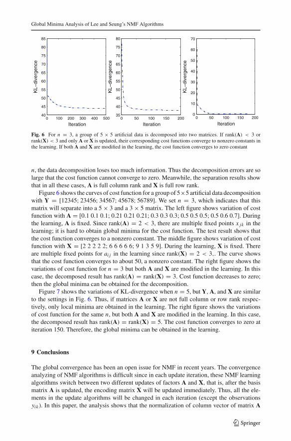
Fig. 6 For n = 3, a group of 5 × 5 artificial data is decomposed into two matrices. If rank(A) < 3 orrank(X) < 3 and only A or X is updated, their corresponding cost functions converge to nonzero constants inthe learning. If both A and X are modified in the learning, the cost function converges to zero constant

n, the data decomposition loses too much information. Thus the decomposition errors are solarge that the cost function cannot converge to zero. Meanwhile, the separation results showthat in all these cases, A is full column rank and X is full row rank.

Figure 6 shows the curves of cost function for a group of 5×5 artificial data decompositionwith Y = [12345; 23456; 34567; 45678; 56789]. We set n = 3, which indicates that thismatrix will separate into a 5× 3 and a 3× 5 matrix. The left figure shows variation of costfunction with A = [0.1 0.1 0.1; 0.21 0.21 0.21; 0.3 0.3 0.3; 0.5 0.5 0.5; 0.5 0.6 0.7]. Duringthe learning, A is fixed. Since rank(A) = 2 < 3, there are multiple fixed points x jk in thelearning; it is hard to obtain global minima for the cost function. The test result shows thatthe cost function converges to a nonzero constant. The middle figure shows variation of costfunction with X = [2 2 2 2 2; 6 6 6 6 6; 9 1 3 5 9]. During the learning, X is fixed. Thereare multiple fixed points for ai j in the learning since rank(X) = 2 < 3,. The curve showsthat the cost function converges to about 50, a nonzero constant. The right figure shows thevariations of cost function for n = 3 but both A and X are modified in the learning. In thiscase, the decomposed result has rank(A) = rank(X) = 3. Cost function decreases to zero;then the global minima can be obtained for the decomposition.

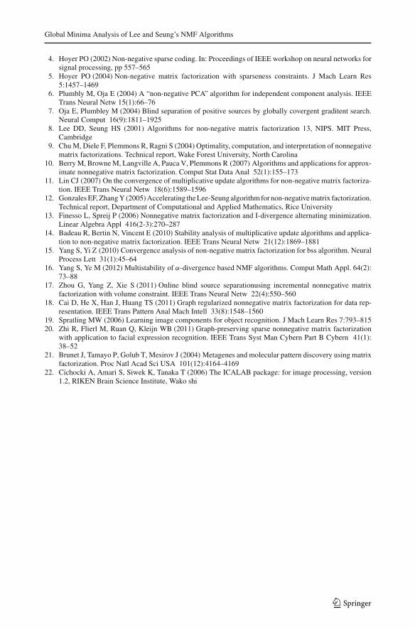
Figure 7 shows the variations of KL-divergence when n = 5, but Y, A, and X are similarto the settings in Fig. 6. Thus, if matrices A or X are not full column or row rank respec-tively, only local minima are obtained in the learning. The right figure shows the variationsof cost function for the same n, but both A and X are modified in the learning. In this case,the decomposed result has rank(A) = rank(X) = 5. The cost function converges to zero atiteration 150. Therefore, the global minima can be obtained in the learning.

9 Conclusions

The global convergence has been an open issue for NMF in recent years. The convergenceanalyzing of NMF algorithms is difficult since in each update iteration, these NMF learningalgorithms switch between two different updates of factors A and X, that is, after the basismatrix A is updated, the encoding matrix X will be updated immediately. Thus, all the ele-ments in the update algorithms will be changed in each iteration (except the observationsyik). In this paper, the analysis shows that the normalization of column vector of matrix A

123

S. Yang, M. Ye

0 50 100 150 20035

40

45

50

55

60

65

70

Iteration

KL−

dive

rgen

ce

0 100 200 300 400 50022

23

24

25

26

27

28

Iteration

KL−

dive

rgen

ce

0 50 100 150 2000

10

20

30

40

50

60

70

Iteration

KL−

dive

rgen

ce

Fig. 7 For n = 5, a group of 5×5 artificial matrix is decomposed into two matrices. When we set rank(A) < 5or rank(X) < 5, their corresponding cost functions converge to nonzero constants in the learning. If both Aand X are modified, the cost function converges to zero constant

is very important. From the analysis, three important results for the NMF algorithms can beachieved.

1. An invariant set (only depends on the observations yik) can be constructed for eachupdate algorithm, thus we can guarantee that all the updates are non-divergent.

2. In the initialization, if we can guarantee that all the elements in A and X to be nonzero,then all the denominator terms in the learning algorithms will not be zeros in the update(without considering the computing errors). Thus, the update algorithms will convergeto their non-zero or zero fixed points.

3. In the practical data decomposition, after the the update finished, usually the decomposedmatrices A is full column rank and X is full row rank, and experiment results show thatwe can obtain the optimized data separation of the cost function.

The NMF algorithms are efficient for extraction and separation of blind sources. However,in the application, it is necessary to choose suitable initializations for the data separation sothat we can guarantee that the update computing will achieve the fixed points of the learningalgorithms since the original cost function is not well-defined. The analysis in this papershows that the NMF algorithms have very good convergence properties in the domain of thelearning algorithms, and the only problem is, if the conditions in Eq. (24), case (24.1) are met,the fixed point does not exist. A large scale data decomposition, it is hard to test the ranksof matrices A and X. However, because of the computing errors, the ranks of decompositionmatrices will always be the minimum number of their row and column. Thus the optimizeddata separation can be obtained by the NMF algorithms

References

1. Lee DD, Seung HS (1999) Learning of the parts of objects by non-negative matrix factorization. Nature401:788–791

2. Cichocki A, Zdunek R, Amari S (2006) New algorithms for non-negative matrix factorization inapplications to blind source separation, ICASSP-2006, Toulouse, pp 621–625

3. Cichocki A, Zdunek R, Amari S (2006) Csiszar’s divergences for non-negative matrix factorization: fam-ily of new algorithms. In: 6th International conference on independent component analysis and blindsignal separation, Springer LNCS 3889, Charleston, pp 32–39

123


4. Hoyer PO (2002) Non-negative sparse coding. In: Proceedings of IEEE workshop on neural networks forsignal processing, pp 557–565

5. Hoyer PO (2004) Non-negative matrix factorization with sparseness constraints. J Mach Learn Res5:1457–1469

6. Plumbly M, Oja E (2004) A “non-negative PCA” algorithm for independent component analysis. IEEETrans Neural Netw 15(1):66–76

7. Oja E, Plumbley M (2004) Blind separation of positive sources by globally covergent graditent search.Neural Comput 16(9):1811–1925

8. Lee DD, Seung HS (2001) Algorithms for non-negative matrix factorization 13, NIPS. MIT Press,Cambridge

9. Chu M, Diele F, Plemmons R, Ragni S (2004) Optimality, computation, and interpretation of nonnegativematrix factorizations. Technical report, Wake Forest University, North Carolina

10. Berry M, Browne M, Langville A, Pauca V, Plemmons R (2007) Algorithms and applications for approx-imate nonnegative matrix factorization. Comput Stat Data Anal 52(1):155–173

11. Lin CJ (2007) On the convergence of multiplicative update algorithms for non-negative matrix factoriza-tion. IEEE Trans Neural Netw 18(6):1589–1596

12. Gonzales EF, Zhang Y (2005) Accelerating the Lee-Seung algorithm for non-negative matrix factorization.Technical report, Department of Computational and Applied Mathematics, Rice University

13. Finesso L, Spreij P (2006) Nonnegative matrix factorization and I-divergence alternating minimization.Linear Algebra Appl 416(2-3):270–287

14. Badeau R, Bertin N, Vincent E (2010) Stability analysis of multiplicative update algorithms and applica-tion to non-negative matrix factorization. IEEE Trans Neural Netw 21(12):1869–1881

15. Yang S, Yi Z (2010) Convergence analysis of non-negative matrix factorization for bss algorithm. NeuralProcess Lett 31(1):45–64

16. Yang S, Ye M (2012) Multistability of α-divergence based NMF algorithms. Comput Math Appl. 64(2):73–88

17. Zhou G, Yang Z, Xie S (2011) Online blind source separationusing incremental nonnegative matrixfactorization with volume constraint. IEEE Trans Neural Netw 22(4):550–560

18. Cai D, He X, Han J, Huang TS (2011) Graph regularized nonnegative matrix factorization for data rep-resentation. IEEE Trans Pattern Anal Mach Intell 33(8):1548–1560

19. Spratling MW (2006) Learning image components for object recognition. J Mach Learn Res 7:793–81520. Zhi R, Flierl M, Ruan Q, Kleijn WB (2011) Graph-preserving sparse nonnegative matrix factorization

with application to facial expression recognition. IEEE Trans Syst Man Cybern Part B Cybern 41(1):38–52

21. Brunet J, Tamayo P, Golub T, Mesirov J (2004) Metagenes and molecular pattern discovery using matrixfactorization. Proc Natl Acad Sci USA 101(12):4164–4169

22. Cichocki A, Amari S, Siwek K, Tanaka T (2006) The ICALAB package: for image processing, version1.2, RIKEN Brain Science Institute, Wako shi

123

Global Minima Analysis of Lee and Seungâs NMF Algorithms

Documents

Transcript of Global Minima Analysis of Lee and Seungâs NMF Algorithms