Global Marine Fuel Trends 2030 - LRQA · Lloyds Register Marine lr.org/marine | University College...

Lloyds Register Marine lr.org/marine | University College London ucl.ac.uk/energy

Global Marine Fuel Trends

2030

Lloyds Register Marine lr.org/marine | University College London ucl.ac.ukGlobal Marine Fuel Trends 2030 Lloyds Register Marine lr.org/marine | University College London ucl.ac.uk/energy02

02 Contents 03 Foreword 04 Executive Summary 08 GloTraM - Global Transport Model 10 Scenarios 12 From Global Marine Trends to Global Marine Fuel Trends 14 Trade scenarios 15 Ship types considered16 Fuels and technologies for deep sea shipping 18 Conventional and alternative fuels 20 Bio-energy 21 Fuel and technology compatibility 22 Energy efficiency technology24 Fuel prices vs. technology cost and performance 26 Fuel price scenarios 28 Technology costs and performance inputs 29 Competitiveness of machinery-fuel combinations30 Marine fuel mix 2030 34 Status Quo 36 Global Commons 38 Competing nations40 EEDI and design vs. operational speeds 46 Marine fuel demand 2030 50 Emissions 2030 52 Emissions accounting framework 53 CO

2 emissions projections to 2030

56 Postscript 57 The GMFT2030 Team 58 Acronyms 59 References

Contents

Acknowledgements and disclaimersThe authors would like to acknowledge the support of their colleagues and management within their organisations in developing this publication.

They would especially like to acknowledge the work of everyone involved in the Low Carbon Shipping Consortium. Their tireless efforts have resulted, among others, in the sophisticated tools and data which are utilised extensively in GMFT2030.

The views expressed in this publication are those of the individuals of the GMFT2030 Team and they do not necessarily reflect the views of the Lloyd’s Register Group Limited (LR), the University College London (UCL) or other members of the Low Carbon Shipping Consortium (LCS).

This publication has been prepared for general guidance on matters of interest only, and does not constitute professional advice. You should not act upon the information contained in this publication without obtaining specific professional advice. No representation or warranty (express or implied) is given as to the accuracy or completeness of the information contained in this publication, and, to the extent permitted by law, Lloyd’s Register Group Limited and University College London do not accept or assume any liability, responsibility or duty of care for any consequences of you or anyone else

acting, or refraining to act, in reliance on the information contained in this publication or for any decision based on it. This publication (and any extract from it) must not be copied, redistributed or placed on any website, without prior written consent.

All trade marks and copyright materials including data, visuals and illustrations are acknowledged as they appear in the document.

Lloyds Register Marine lr.org/marine | University College London ucl.ac.ukLloyds Register Marine lr.org/marine | University College London ucl.ac.uk/energy 03

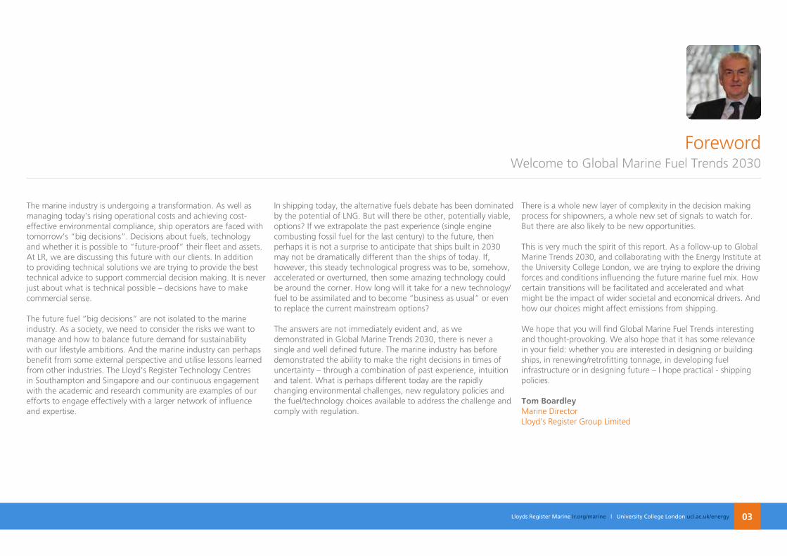
The marine industry is undergoing a transformation. As well as managing today’s rising operational costs and achieving cost-effective environmental compliance, ship operators are faced with tomorrow’s “big decisions”. Decisions about fuels, technology and whether it is possible to “future-proof” their fleet and assets. At LR, we are discussing this future with our clients. In addition to providing technical solutions we are trying to provide the best technical advice to support commercial decision making. It is never just about what is technical possible – decisions have to make commercial sense.

The future fuel “big decisions” are not isolated to the marine industry. As a society, we need to consider the risks we want to manage and how to balance future demand for sustainability with our lifestyle ambitions. And the marine industry can perhaps benefit from some external perspective and utilise lessons learned from other industries. The Lloyd’s Register Technology Centres in Southampton and Singapore and our continuous engagement with the academic and research community are examples of our efforts to engage effectively with a larger network of influence and expertise.

In shipping today, the alternative fuels debate has been dominated by the potential of LNG. But will there be other, potentially viable, options? If we extrapolate the past experience (single engine combusting fossil fuel for the last century) to the future, then perhaps it is not a surprise to anticipate that ships built in 2030 may not be dramatically different than the ships of today. If, however, this steady technological progress was to be, somehow, accelerated or overturned, then some amazing technology could be around the corner. How long will it take for a new technology/fuel to be assimilated and to become “business as usual” or even to replace the current mainstream options?

The answers are not immediately evident and, as we demonstrated in Global Marine Trends 2030, there is never a single and well defined future. The marine industry has before demonstrated the ability to make the right decisions in times of uncertainty – through a combination of past experience, intuition and talent. What is perhaps different today are the rapidly changing environmental challenges, new regulatory policies and the fuel/technology choices available to address the challenge and comply with regulation.

There is a whole new layer of complexity in the decision making process for shipowners, a whole new set of signals to watch for. But there are also likely to be new opportunities.

This is very much the spirit of this report. As a follow-up to Global Marine Trends 2030, and collaborating with the Energy Institute at the University College London, we are trying to explore the driving forces and conditions influencing the future marine fuel mix. How certain transitions will be facilitated and accelerated and what might be the impact of wider societal and economical drivers. And how our choices might affect emissions from shipping.

We hope that you will find Global Marine Fuel Trends interesting and thought-provoking. We also hope that it has some relevance in your field: whether you are interested in designing or building ships, in renewing/retrofitting tonnage, in developing fuel infrastructure or in designing future – I hope practical - shipping policies.

Tom BoardleyMarine DirectorLloyd’s Register Group Limited

ForewordWelcome to Global Marine Fuel Trends 2030


Global Marine Fuel Trends 2030 central objective is to unravel the landscape of fuels used by commercial shipping over the next 16 years. The problem has many dimensions: a fuel needs to be available, cost-effective, compatible with existing and future technology and compliant with current and future environmental requirements. In a way, one cannot evaluate the future of marine fuels without evaluating the future of the marine industry. And the future of the marine industry itself is irrevocably linked with the global economic, social and political landscape to 2030.

Rather than looking for a single outcome, we use scenario planning methodologies. This is why we are making the connection with Global Marine Trends 2030, through its 3 different scenarios: Status Quo, Global Commons and Competing Nations.

These scenarios represent alternative futures for the world and shipping in 2030, from business as usual to more globalisation or more localisation. Our assumptions are fed into probably the most sophisticated scenario planning model that exists for global shipping, GloTraM, developed as part of the Low Carbon Shipping Consortium. The model analyses how the global fleet evolves in response to external drivers such as fuel prices, transport demand and technology availability, cost and technical compatibility. Tonnage replacement and design/operational speeds are adjusted to ensure a balance between transport demand and supply. The decision-making algorithms in the model are based in the principles of regulatory compliance and ship-owner profit-maximisation, very much aligned to the dimensions of the future fuel challenge.

GMFT 2030 boundaries are wide but not completely inclusive: we examine the containership, bulk carrier/general cargo and tanker (crude and chemical/products) sectors, representing approximately 70% of the shipping industry’s fuel demand in 2007. We include fuels ranging from liquid fuels used today (HFO, MDO/MGO) to their bio-alternatives (bio-diesel, straight vegetable oil) and from LNG and biogas to methanol and hydrogen (derived both from methane or wood biomass). Engine technology includes 2 or 4 stroke diesels, diesel-electric, gas engines and fuel cell technology. A wide range of energy efficiency technologies and abatement solutions (including sulphur scrubbers and Selective Catalytic Reduction for NOx emissions abatement) compatible with the examined ship types are included in the modelling. The uptake of these technologies influences the uptake of different fuels.

Regulation is aligned with each of the 3 overarching scenarios to reflect business-as-usual, globalisation or localisation trends. They include current and future emission control areas (ECAs), energy efficiency requirements (EEDI) and carbon policies (carbon tax). Oil, gas and hydrogen fuel prices are also linked to the Status Quo, Global Commons and Competing Nations scenarios.

So what does the marine fuel mix look like for containers, bulk carriers and tankers by 2030? In two words: decreasingly conventional. HFO will still be very much around in 2030, but in different proportions for each scenario: 47% in Status Quo, to a higher 66% in Competing Nations and a 58% in Global Commons. A high share of HFO means a high uptake of emissions abatement technology.

Executive Summary

One cannot evaluate the future of marine fuels without evaluating the future of the marine industry

We examine the containership, bulk carrier/general cargo and tanker sectors, representing approximately 70% of the fuel demand in 2007


The space left by the declining share of HFO will be filled by low sulphur alternatives (MDO/MGO or LSHFO) and by LNG, and this will happen differently for each ship type and scenario. LNG will reach a maximum 11% share by 2030 in Status Quo. There is also the entry of Hydrogen as an emerging shipping fuel in 2030 Global Commons, a scenario which favours the uptake of low carbon technologies stimulated by a significant carbon price.

Contrary to common perceptions, containerships are not the segment with the highest share of LNG - in fact it is the chemical/product tankers, with LNG making up 31% of its fuel mix by 2030 in Status Quo. In contrast, containerships will see a maximum 5% LNG share in Global Commons. This can be explained considering that the fuel mix represents the entire fleet, so tonnage age and renewal are as important as technical compatibility and cost-effectiveness of different fuels.

Segments with the higher proportion of small ships see the highest LNG uptake. It is also a matter of perspective: from a non-existent share of the marine market in 2010, LNG will have 5-10% share in 20 years. We are not saying that LNG will not be the fuel of the future. But that seeing new ships built with LNG today (many of which in niche markets/short-sea shipping) and overturning the marine fuel landscape in less than a ship’s lifetime are two entirely different discussions. Methanol does not appear in the fuel mix in any considerable quantities by 2030. It may be that this timeframe is too short or that it is not a cost-effective solution making it, again, appropriate for a niche market not represented by the 4 main ship types we examined.

While the fuel mix indicates a declining share of HFO, filled by alternative options, in 2030 the demand for HFO will be at least the same (In Status Quo) if not 23% higher (in Global Commons) compared to its 2010 levels. But, with the overall fuel demand doubling by 2030, other fuels will see a higher rate of growth to meet this demand.

The fuel choice and scenarios are shown to create differences in energy efficiency technology take-up, design and operating speed. Low technology take-up occurs in Status Quo and Competing Nations, although installed power reduces due to reductions in design speed. Greater installed power reduction occurs in Global Commons, due to the combination of design speed reductions and greater efficiency technology take-up.

Typically, the installed power in Global Commons is operated at higher engine loads, resulting in marginally higher average operating speeds when compared with the other scenarios. This is due to the greater technical efficiency of the Global Commons fleet. As the most profitable fuel and machinery change over time and between scenario, this in turn impacts the optimum operating speed, with higher fuel prices and less energy efficient (e.g. older) ships operating at lower speeds when compared with the newer ships of the same ship type and size.

LNG will reach a maximum 11% share in 2030. Segments with the higher proportion of small ships will see the highest LNG uptake

HFO will still be very much around in 2030, taking 47%-66% of the fuel mix


The fuel mix may be a central output to this study but it is not the only one. GloTraM can predict shipping emissions and these are very much affected by the same drivers that we already discussed plus the marine fuel mix itself. Despite improvements in design and operational efficiency and current/future policies, CO2 emissions from shipping will not decrease in 2030. Status Quo will see its emissions doubling, due to the increase in trade volume combined with the moderate carbon policy and the low uptake of low carbon fuels. Global Commons is following a similar trend but then decreasing post 2025, thanks to carbon policy and the uptake of Hydrogen. Competing nations will see the smallest growth in emissions.

Despite the lack of carbon policy, the smaller trade volume, high energy prices and, predominantly, the high uptake of bio-energy, result in the lowest increase of CO2 emissions than any other scenario (56%).

The lower emissions associated with this scenario seem attractive but come at the cost of lower growth in the shipping industry, higher operating costs and less global trade. Furthermore, in 2030, in Competing Nations and Status Quo, emissions remain on an upwards trajectory and the global fleet remains similar to the fleet in 2010 with the industry poorly positioned to weather any policy or macroeconomic storms in the period 2030-2050. In contrast, in Global Commons the sector’s emissions peak (in 2025) and are starting a downwards trajectory that should assist in a more stable and sustainable long-term growth in shipping, trade growth and global economic development.

When discussing future policies and shipping CO2 emissions, it is worth considering our assumptions for calculating them, which is that GHG emissions come from the CO2 released in fuel combustion activities of the vessels during their operation. However, if LNG, bio-fuels and hydrogen take a greater role in the shipping, it would be important to consider emissions associated with upstream processes and for non-CO2 emissions, for example methane slip. This could show that fuels which, on the basis of operational emissions alone, appear attractive have significant wider impacts. This is important when developing mitigation policies.

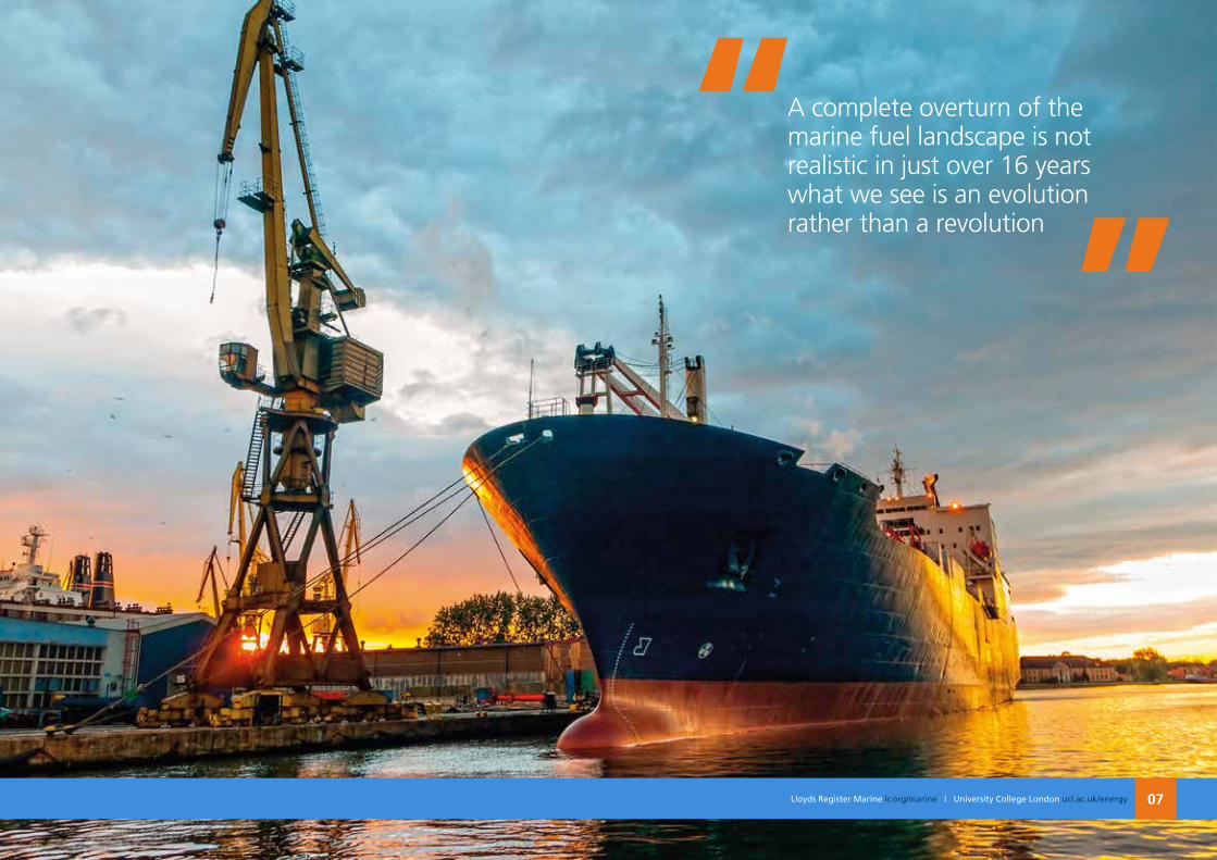
Having looked at a variety of fuels, technologies, economic and regulation scenarios, all resulting in different future outcomes, what is perhaps the main take-away from GMFT2030? We often talk about tipping points but what we anticipate is an evolutionary process rather than any instant shift. 16 years is less than a ship’s lifetime and a dramatic overturn of the marine fuel landscape may not be realistic. On the other hand, it is also a matter of perspective: we may not see an immediate revolution but we will certainly experience some changing trends.

In Status Quo, shipping emissions will double by 2030. Carbon policies result to a downwards trajectory in Global Commons

If alternative fuels take a greater role in shipping, it is important to consider upstream emissions beyond the point of operation


A complete overturn of the marine fuel landscape is not realistic in just over 16 years what we see is an evolution rather than a revolution


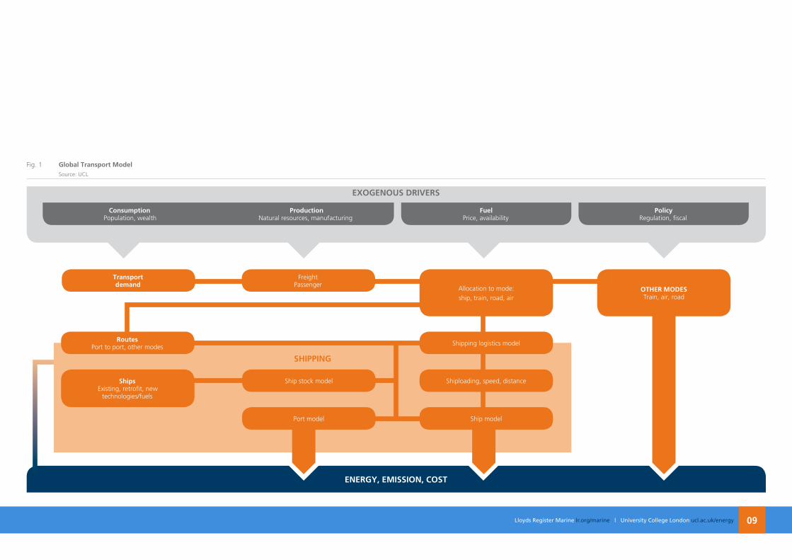
GMFT2030 uses the Global Transport Model (GloTraM) to analyse the role and demand for different fuels and technologies. GloTraM combines multi-disciplinary analysis and modelling techniques to estimate foreseeable futures of the shipping industry. The model starts with a definition of the global shipping system in a baseline year (2010) and then evolves the fleet and its activity in response to external drivers (changing fuel prices, transport demand, regulation and technology availability).

GloTraM undertakes a rigorous analysis of the existing fleet, along with the economics of technology investment and operation in the shipping industry. This approach ensures that the model closely resembles the behaviour of the stakeholders within the shipping industry and their decision-making processes to ensure realistic simulation of their likely response to external factors such as a carbon price. The decision-making process to determine technical and operational specifications of new build and existing ships are driven by the shipowner’s profit maximisation and regulatory compliance.

An important feature of GloTraM is its representation of the interaction between technical and operational specifications and the inclusion of technology additionality and compatibility. For example, some technologies are optimised for a given “design speed” but their savings may reduce as operating speed reduces or increases, or that there could be incompatibilities between certain exhaust treatment solutions (wet scrubbers) and engine efficiency modifications (waste heat recovery). Other examples include the interaction between speed and wind assistance fuel savings (higher % of fuel saved for lower average speeds), or the incompatibility of certain combinations of hydrodynamic devices that might be used to improve the flow through the propeller and over the control surfaces. These interactions are often overlooked using conventional marginal abatement cost curve based approaches but are taken into account within GloTraM.

Another important element of GloTraM is the attention paid to characterising the fleet’s operational parameters in the baseline year. In 2010, a large number of ships were slow steaming due to the conditions in the shipping markets. This affects both energy demands and the energy and cost savings potentials of technology. Satellite AIS data is used to produce calibrations of the operational speeds in each ship type and size category for the baseline year, and operational speed is modified at each time-step as a function of the evolving market conditions and fuel prices. More details on this approach can be found on the report “Assessment of Shipping’s Efficiency Using Satellite AIS data” (Smith, et al., 2013d).

GloTraM was initially developed by the RCUK Energy programme and the industry funded project “Low Carbon Shipping – A Systems Approach”, which Lloyd’s Register and UCL are members among other industry partners, NGOs and universities.

www.lowcarbonshipping.co.uk

GloTraM - Global Transport Model

Lloyds Register Marine lr.org/marine | University College London ucl.ac.uk

EnERGy, EMISSIon, CoST

EXoGEnoUS DRIVERS

Lloyds Register Marine lr.org/marine | University College London ucl.ac.uk/energy 09

Fig. 1 Global Transport Model Source: UCL

ConsumptionPopulation, wealth

ProductionNatural resources, manufacturing

FuelPrice, availability

Transport demand

Freight Passenger

PolicyRegulation, fiscal

SHIPPInG

RoutesPort to port, other modes

ShipsExisting, retrofit, new

technologies/fuels

Port model

Ship stock model

oTHER MoDESTrain, air, road

Shipping logistics model

Shiploading, speed, distance

Ship model

Allocation to mode:

ship, train, road, air


Scenarios


Economic and popultion growth

International cooperation vs. protectionism

Oil and gas price trajectories

Bio-energy scenarios

Profitablity of fuel/machinery

combinations

Emissions projections

Global Marine Fuel Trends 2030 Lloyds Register Marine lr.org/marine | University College London ucl.ac.uk/energy12

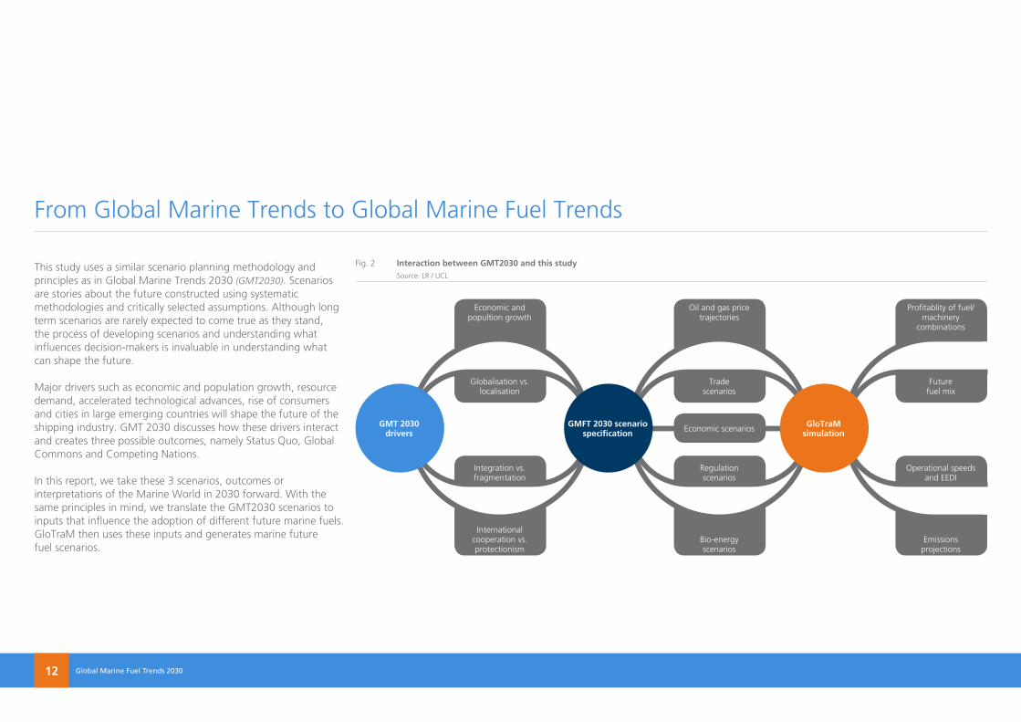
This study uses a similar scenario planning methodology and principles as in Global Marine Trends 2030 (GMT2030). Scenarios are stories about the future constructed using systematic methodologies and critically selected assumptions. Although long term scenarios are rarely expected to come true as they stand, the process of developing scenarios and understanding what influences decision-makers is invaluable in understanding what can shape the future.

Major drivers such as economic and population growth, resource demand, accelerated technological advances, rise of consumers and cities in large emerging countries will shape the future of the shipping industry. GMT 2030 discusses how these drivers interact and creates three possible outcomes, namely Status Quo, Global Commons and Competing Nations.

In this report, we take these 3 scenarios, outcomes or interpretations of the Marine World in 2030 forward. With the same principles in mind, we translate the GMT2030 scenarios to inputs that influence the adoption of different future marine fuels. GloTraM then uses these inputs and generates marine future fuel scenarios.

From Global Marine Trends to Global Marine Fuel Trends

Fig. 2 Interaction between GMT2030 and this study Source: LR / UCL

GMT 2030 drivers

GMFT 2030 scenario specification

GloTraM simulation

Globalisation vs. localisation

Integration vs. fragmentation

Trade scenarios

Regulation scenarios

Future fuel mix

Operational speeds and EEDI

Economic scenarios


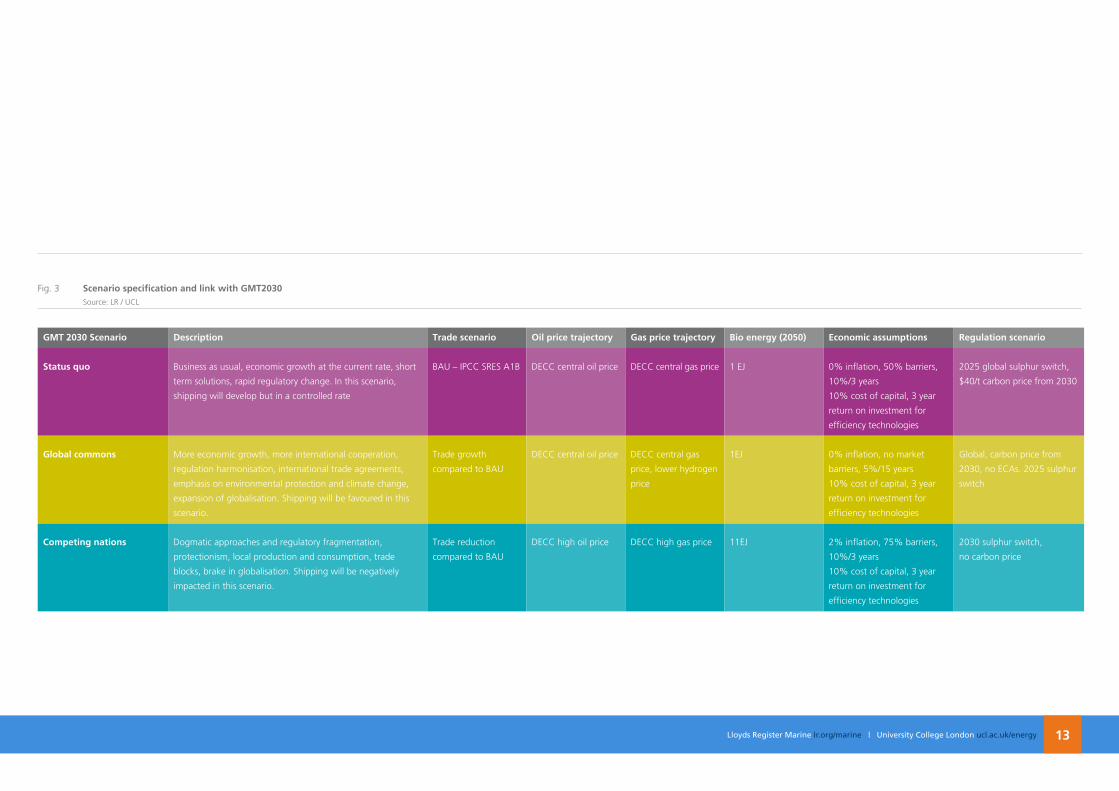
GMT 2030 Scenario Description Trade scenario oil price trajectory Gas price trajectory Bio energy (2050) Economic assumptions Regulation scenario

Status quo Business as usual, economic growth at the current rate, short

term solutions, rapid regulatory change. In this scenario,

shipping will develop but in a controlled rate

BAU – IPCC SRES A1B DECC central oil price DECC central gas price 1 EJ 0% inflation, 50% barriers,

10%/3 years

10% cost of capital, 3 year

return on investment for

efficiency technologies

2025 global sulphur switch,

$40/t carbon price from 2030

Global commons More economic growth, more international cooperation,

regulation harmonisation, international trade agreements,

emphasis on environmental protection and climate change,

expansion of globalisation. Shipping will be favoured in this

scenario.

Trade growth

compared to BAU

DECC central oil price DECC central gas

price, lower hydrogen

price

1EJ 0% inflation, no market

barriers, 5%/15 years




Global, carbon price from

2030, no ECAs. 2025 sulphur

switch

Competing nations Dogmatic approaches and regulatory fragmentation,

protectionism, local production and consumption, trade

blocks, brake in globalisation. Shipping will be negatively

impacted in this scenario.

Trade reduction

compared to BAU

DECC high oil price DECC high gas price 11EJ 2% inflation, 75% barriers,

10%/3 years




2030 sulphur switch,

no carbon price

Fig. 3 Scenario specification and link with GMT2030 Source: LR / UCL


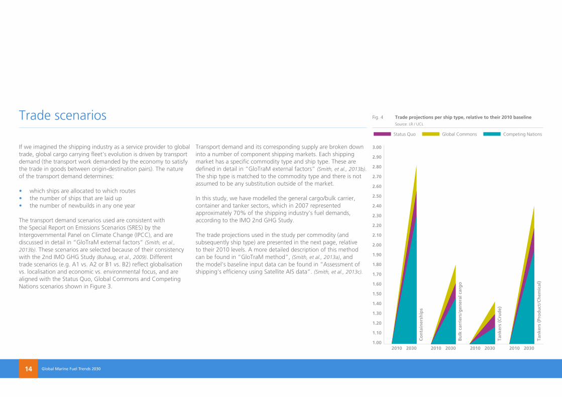
If we imagined the shipping industry as a service provider to global trade, global cargo carrying fleet’s evolution is driven by transport demand (the transport work demanded by the economy to satisfy the trade in goods between origin-destination pairs). The nature of the transport demand determines:

• which ships are allocated to which routes• the number of ships that are laid up• the number of newbuilds in any one year

The transport demand scenarios used are consistent with the Special Report on Emissions Scenarios (SRES) by the Intergovernmental Panel on Climate Change (IPCC), and are discussed in detail in “GloTraM external factors” (Smith, et al., 2013b). These scenarios are selected because of their consistency with the 2nd IMO GHG Study (Buhaug, et al., 2009). Different trade scenarios (e.g. A1 vs. A2 or B1 vs. B2) reflect globalisation vs. localisation and economic vs. environmental focus, and are aligned with the Status Quo, Global Commons and Competing Nations scenarios shown in Figure 3.

Transport demand and its corresponding supply are broken down into a number of component shipping markets. Each shipping market has a specific commodity type and ship type. These are defined in detail in “GloTraM external factors” (Smith, et al., 2013b). The ship type is matched to the commodity type and there is not assumed to be any substitution outside of the market.

In this study, we have modelled the general cargo/bulk carrier, container and tanker sectors, which in 2007 represented approximately 70% of the shipping industry’s fuel demands, according to the IMO 2nd GHG Study.

The trade projections used in the study per commodity (and subsequently ship type) are presented in the next page, relative to their 2010 levels. A more detailed description of this method can be found in “GloTraM method”, (Smith, et al., 2013a), and the model’s baseline input data can be found in “Assessment of shipping’s efficiency using Satellite AIS data”. (Smith, et al., 2013c).

Trade scenarios Fig. 4 Trade projections per ship type, relative to their 2010 baseline Source: LR / UCL

Status Quo Global Commons Competing Nations

1.00

1.20

2.20

1.40

2.40

1.70

2.70

1.10

2.10

1.30

2.30

1.60

2.60

1.50

2.50

1.80

2.80

1.90

2.90

2.00

3.00

2010 2030 2010 2030 2010 2030 2010 2030

Co

nta

iner

ship

s

Bu

lk c

arri

ers/

gen

eral

car

go

Tan

kers

(C

rud

e)

Tan

kers

(Pr

od

uct

/Ch

emic

al)


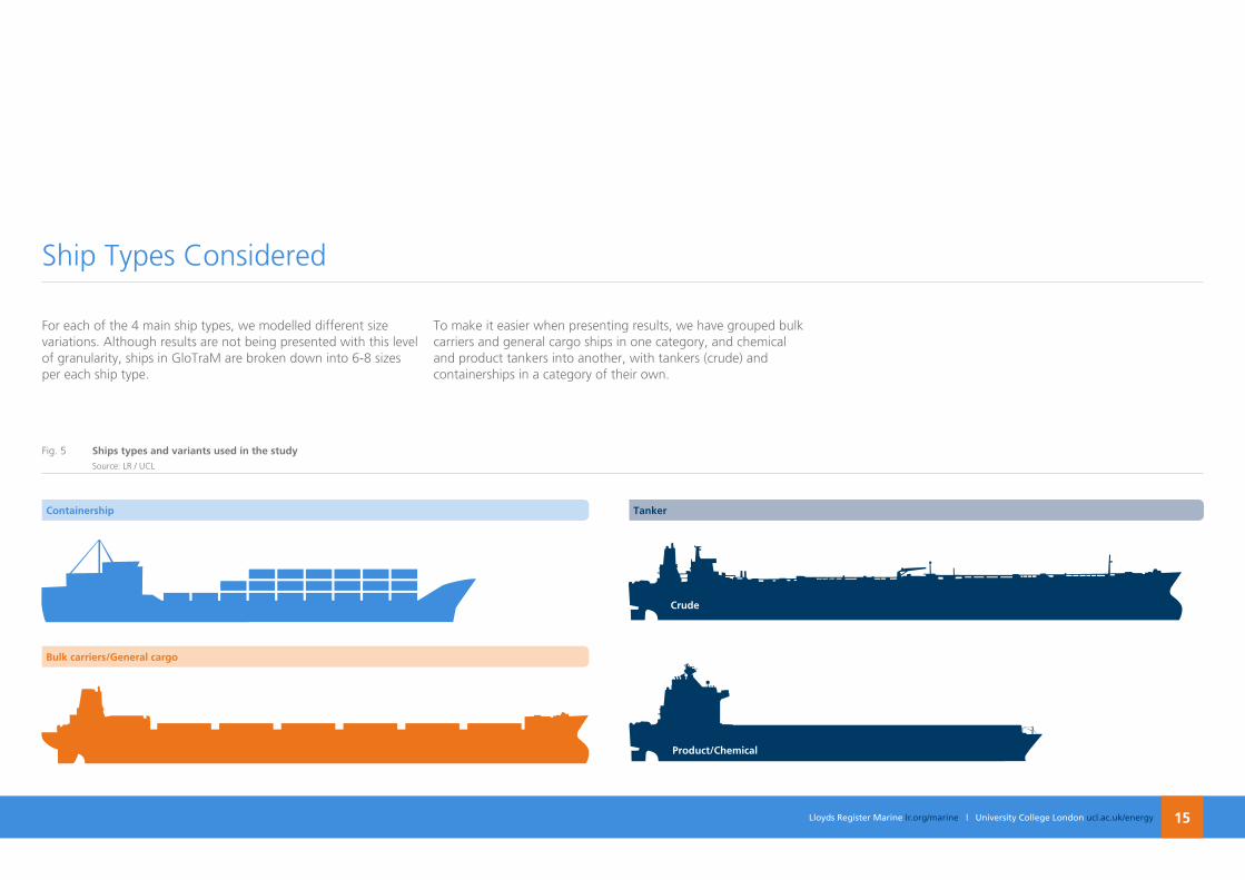
For each of the 4 main ship types, we modelled different size variations. Although results are not being presented with this level of granularity, ships in GloTraM are broken down into 6-8 sizes per each ship type.

To make it easier when presenting results, we have grouped bulk carriers and general cargo ships in one category, and chemical and product tankers into another, with tankers (crude) and containerships in a category of their own.

Ship Types Considered

Fig. 5 Ships types and variants used in the study Source: LR / UCL

Bulk carriers/General cargo

TankerContainership

Crude

Product/Chemical


Fuels and technologies for deep sea shipping


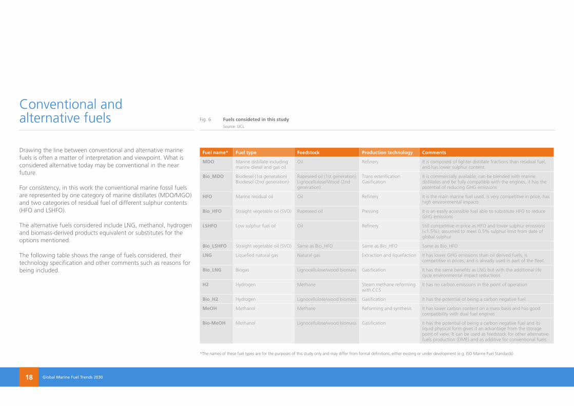
Drawing the line between conventional and alternative marine fuels is often a matter of interpretation and viewpoint. What is considered alternative today may be conventional in the near future.

For consistency, in this work the conventional marine fossil fuels are represented by one category of marine distillates (MDO/MGO) and two categories of residual fuel of different sulphur contents (HFO and LSHFO).

The alternative fuels considered include LNG, methanol, hydrogen and biomass-derived products equivalent or substitutes for the options mentioned.

The following table shows the range of fuels considered, their technology specification and other comments such as reasons for being included.

*The names of these fuel types are for the purposes of this study only and may differ from formal definitions, either existing or under development (e.g. ISO Marine Fuel Standards)

Fuel name* Fuel type Feedstock Production technology Comments

MDo Marine distillate including marine diesel and gas oil

Oil Refinery It is composed of lighter distillate fractions than residual fuel, and has lower sulphur content.

Bio_MDo Biodiesel (1st generation)Biodiesel (2nd generation)

Rapeseed oil (1st generation)Lignocellulose/Wood (2nd generation)

Trans esterification Gasification

It is commercially available, can be blended with marine distillates and be fully compatible with the engines, it has the potential of reducing GHG emissions

HFo Marine residual oil Oil Refinery It is the main marine fuel used, is very competitive in price, has high environmental impacts

Bio_HFo Straight vegetable oil (SVO) Rapeseed oil Pressing It is an easily accessible fuel able to substitute HFO to reduce GHG emissions

LSHFo Low sulphur fuel oil Oil Refinery Still competitive in price as HFO and lower sulphur emissions (<1.5%), assumed to meet 0.5% sulphur limit from date of global sulphur

Bio_LSHFo Straight vegetable oil (SVO) Same as Bio_HFO Same as Bio_HFO Same as Bio_HFO

LnG Liquefied natural gas Natural gas Extraction and liquefaction It has lower GHG emissions than oil derived fuels, is competitive in prices, and is already used in part of the fleet.

Bio_LnG Biogas Lignocellulose/wood biomass Gasification It has the same benefits as LNG but with the additional life cycle environmental impact reductions.

H2 Hydrogen Methane Steam methane reforming with CCS

It has no carbon emissions in the point of operation

Bio_H2 Hydrogen Lignocellulose/wood biomass Gasification It has the potential of being a carbon negative fuel.

MeoH Methanol Methane Reforming and synthesis It has lower carbon content on a mass basis and has good compatibility with dual fuel engines

Bio-MeoH Methanol Lignocellulose/wood biomass Gasification It has the potential of being a carbon negative fuel and its liquid physical form gives it an advantage from the storage point of view. It can be used as feedstock for other alternative fuels production (DME) and as additive for conventional fuels.

Conventional and alternative fuels Fig. 6 Fuels consideted in this study

Source: UCL


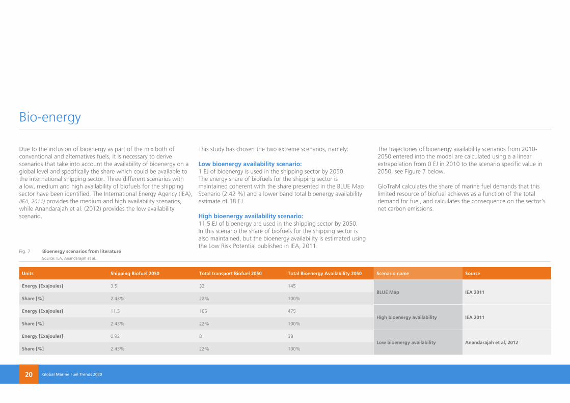
Due to the inclusion of bioenergy as part of the mix both of conventional and alternatives fuels, it is necessary to derive scenarios that take into account the availability of bioenergy on a global level and specifically the share which could be available to the international shipping sector. Three different scenarios with a low, medium and high availability of biofuels for the shipping sector have been identified. The International Energy Agency (IEA), (IEA, 2011) provides the medium and high availability scenarios, while Anandarajah et al. (2012) provides the low availability scenario.

This study has chosen the two extreme scenarios, namely:

Low bioenergy availability scenario: 1 EJ of bioenergy is used in the shipping sector by 2050. The energy share of biofuels for the shipping sector is maintained coherent with the share presented in the BLUE Map Scenario (2.42 %) and a lower band total bioenergy availability estimate of 38 EJ.

High bioenergy availability scenario: 11.5 EJ of bioenergy are used in the shipping sector by 2050. In this scenario the share of biofuels for the shipping sector is also maintained, but the bioenergy availability is estimated using the Low Risk Potential published in IEA, 2011.

The trajectories of bioenergy availability scenarios from 2010-2050 entered into the model are calculated using a a linear extrapolation from 0 EJ in 2010 to the scenario specific value in 2050, see Figure 7 below.

GloTraM calculates the share of marine fuel demands that this limited resource of biofuel achieves as a function of the total demand for fuel, and calculates the consequence on the sector’s net carbon emissions.

Units Shipping Biofuel 2050 Total transport Biofuel 2050 Total Bioenergy Availability 2050 Scenario name Source

Energy [Exajoules] 3.5 32 145BLUE Map IEA 2011

Share [%] 2.43% 22% 100%

Energy [Exajoules] 11.5 105 475High bioenergy availability IEA 2011

Share [%] 2.43% 22% 100%

Energy [Exajoules] 0.92 8 38Low bioenergy availability Anandarajah et al, 2012

Share [%] 2.43% 22% 100%

Bio-energy

Fig. 7 Bioenergy scenarios from literature Source: IEA, Anandarajah et al.


HFO MDO/ MGO LSHFO LNG Hydrogen Methanol


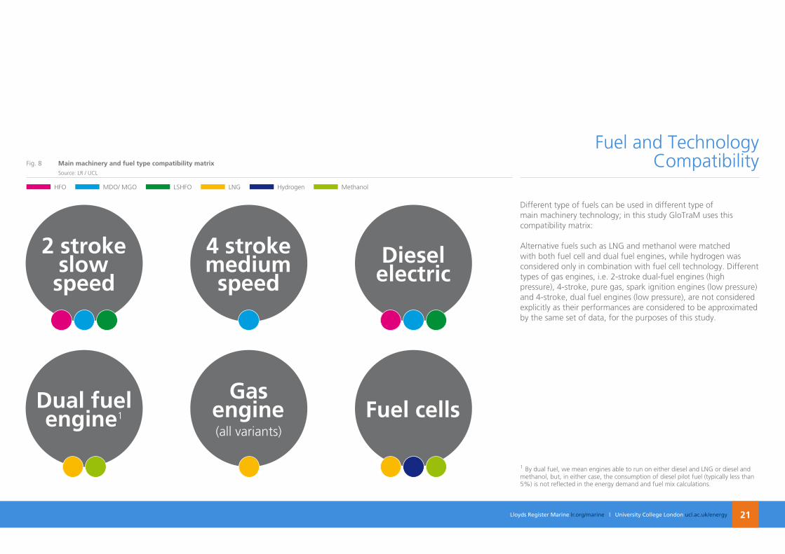
Different type of fuels can be used in different type of main machinery technology; in this study GloTraM uses this compatibility matrix:

Alternative fuels such as LNG and methanol were matched with both fuel cell and dual fuel engines, while hydrogen was considered only in combination with fuel cell technology. Different types of gas engines, i.e. 2-stroke dual-fuel engines (high pressure), 4-stroke, pure gas, spark ignition engines (low pressure) and 4-stroke, dual fuel engines (low pressure), are not considered explicitly as their performances are considered to be approximated by the same set of data, for the purposes of this study.

1 By dual fuel, we mean engines able to run on either diesel and LNG or diesel and methanol, but, in either case, the consumption of diesel pilot fuel (typically less than 5%) is not reflected in the energy demand and fuel mix calculations.

Fuel and Technology Compatibility

2 stroke slow speed

Dual fuel engine1

4 stroke medium speed

Gas engine (all variants)

Diesel electric

Fuel cells

Fig. 8 Main machinery and fuel type compatibility matrix Source: LR / UCL


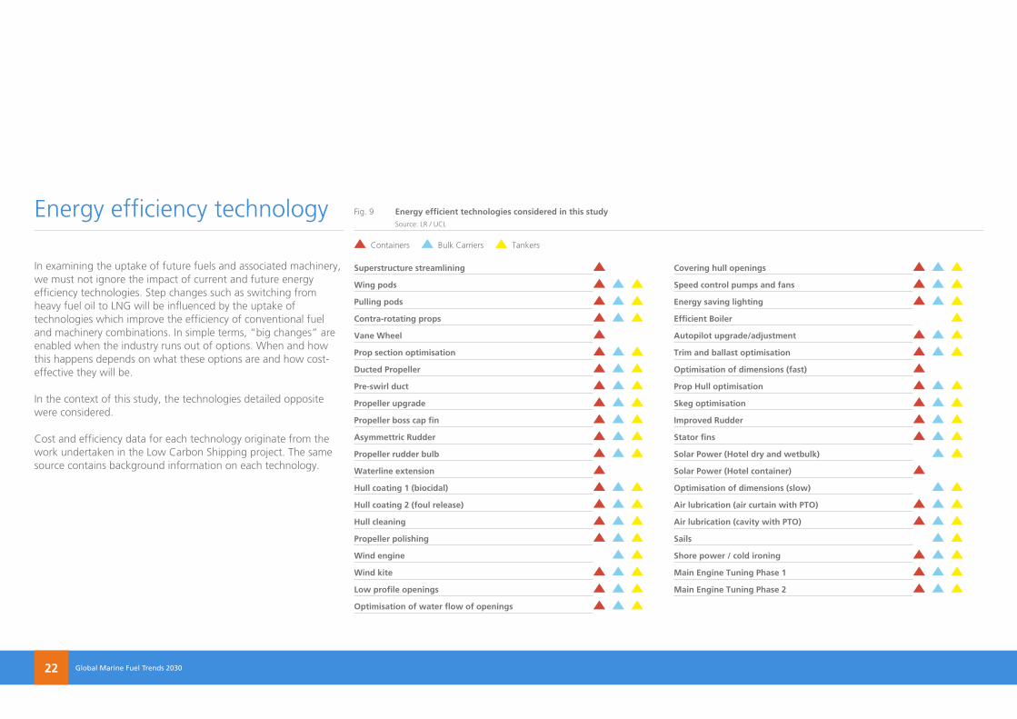
In examining the uptake of future fuels and associated machinery, we must not ignore the impact of current and future energy efficiency technologies. Step changes such as switching from heavy fuel oil to LNG will be influenced by the uptake of technologies which improve the efficiency of conventional fuel and machinery combinations. In simple terms, “big changes” are enabled when the industry runs out of options. When and how this happens depends on what these options are and how cost-effective they will be.

In the context of this study, the technologies detailed opposite were considered.

Cost and efficiency data for each technology originate from the work undertaken in the Low Carbon Shipping project. The same source contains background information on each technology.

Superstructure streamlining

Wing pods

Pulling pods

Contra-rotating props

Vane Wheel

Prop section optimisation

Ducted Propeller

Pre-swirl duct

Propeller upgrade

Propeller boss cap fin

Asymmettric Rudder

Propeller rudder bulb

Waterline extension

Hull coating 1 (biocidal)

Hull coating 2 (foul release)

Hull cleaning

Propeller polishing

Wind engine

Wind kite

Low profile openings

optimisation of water flow of openings

Covering hull openings

Speed control pumps and fans

Energy saving lighting

Efficient Boiler

Autopilot upgrade/adjustment

Trim and ballast optimisation

optimisation of dimensions (fast)

Prop Hull optimisation

Skeg optimisation

Improved Rudder

Stator fins

Solar Power (Hotel dry and wetbulk)

Solar Power (Hotel container)

optimisation of dimensions (slow)

Air lubrication (air curtain with PTo)

Air lubrication (cavity with PTo)

Sails

Shore power / cold ironing

Main Engine Tuning Phase 1

Main Engine Tuning Phase 2

Energy efficiency technology Fig. 9 Energy efficient technologies considered in this study Source: LR / UCL

Containers Bulk Carriers Tankers


Fuel prices vs. technology cost and performance


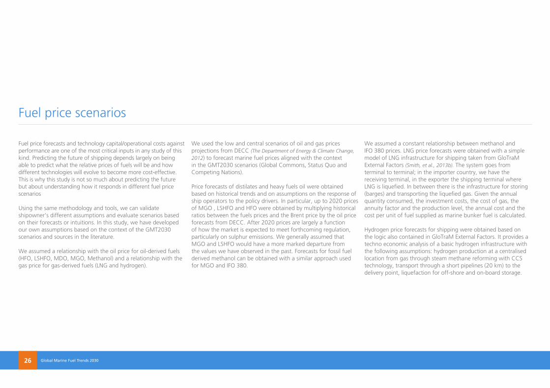
Fuel price forecasts and technology capital/operational costs against performance are one of the most critical inputs in any study of this kind. Predicting the future of shipping depends largely on being able to predict what the relative prices of fuels will be and how different technologies will evolve to become more cost-effective. This is why this study is not so much about predicting the future but about understanding how it responds in different fuel price scenarios

Using the same methodology and tools, we can validate shipowner’s different assumptions and evaluate scenarios based on their forecasts or intuitions. In this study, we have developed our own assumptions based on the context of the GMT2030 scenarios and sources in the literature.

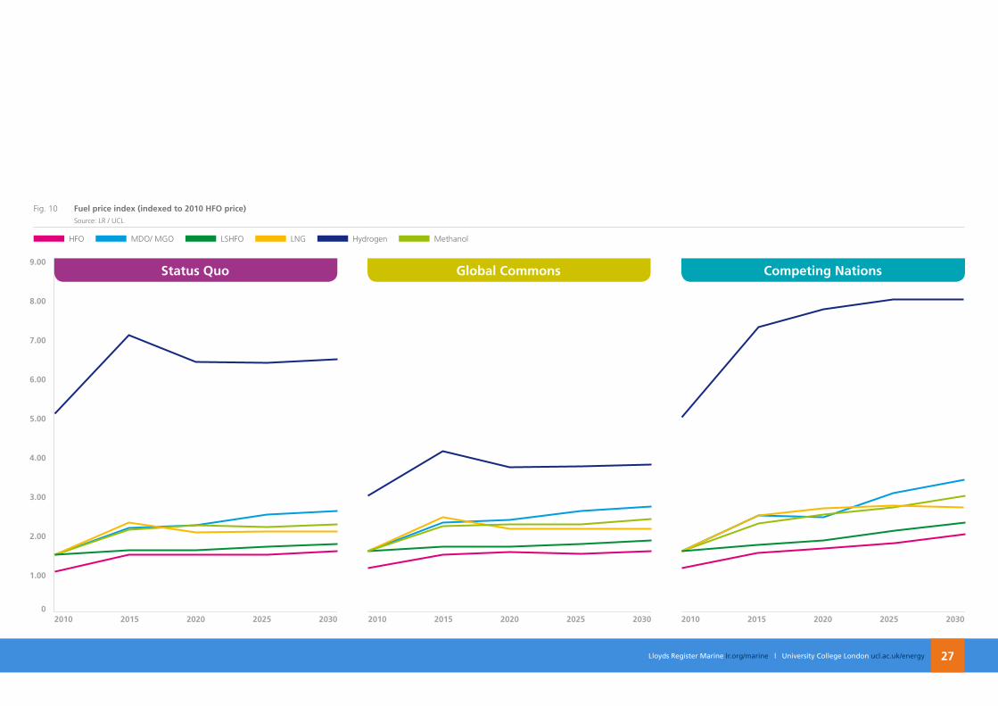
We assumed a relationship with the oil price for oil-derived fuels (HFO, LSHFO, MDO, MGO, Methanol) and a relationship with the gas price for gas-derived fuels (LNG and hydrogen).

We used the low and central scenarios of oil and gas prices projections from DECC (The Department of Energy & Climate Change, 2012) to forecast marine fuel prices aligned with the context in the GMT2030 scenarios (Global Commons, Status Quo and Competing Nations).

Price forecasts of distilates and heavy fuels oil were obtained based on historical trends and on assumptions on the response of ship operators to the policy drivers. In particular, up to 2020 prices of MGO , LSHFO and HFO were obtained by multiplying historical ratios between the fuels prices and the Brent price by the oil price forecasts from DECC. After 2020 prices are largely a function of how the market is expected to meet forthcoming regulation, particularly on sulphur emissions. We generally assumed that MGO and LSHFO would have a more marked departure from the values we have observed in the past. Forecasts for fossil fuel derived methanol can be obtained with a similar approach used for MGO and IFO 380.

We assumed a constant relationship between methanol and IFO 380 prices. LNG price forecasts were obtained with a simple model of LNG infrastructure for shipping taken from GloTraM External Factors (Smith, et al., 2013b). The system goes from terminal to terminal; in the importer country, we have the receiving terminal, in the exporter the shipping terminal where LNG is liquefied. In between there is the infrastructure for storing (barges) and transporting the liquefied gas. Given the annual quantity consumed, the investment costs, the cost of gas, the annuity factor and the production level, the annual cost and the cost per unit of fuel supplied as marine bunker fuel is calculated.

Hydrogen price forecasts for shipping were obtained based on the logic also contained in GloTraM External Factors. It provides a techno economic analysis of a basic hydrogen infrastructure with the following assumptions: hydrogen production at a centralised location from gas through steam methane reforming with CCS technology, transport through a short pipelines (20 km) to the delivery point, liquefaction for off-shore and on-board storage.

Fuel price scenarios


Status Quo Global Commons

HFO MDO/ MGO LSHFO LNG Hydrogen Methanol

Competing nations


Fig. 10 Fuel price index (indexed to 2010 HFo price) Source: LR / UCL

2010 2030202520202015 2010 2030202520202015 2010 20302025202020150

1.00

6.00

5.00

4.00

3.00

2.00

9.00

7.00

8.00


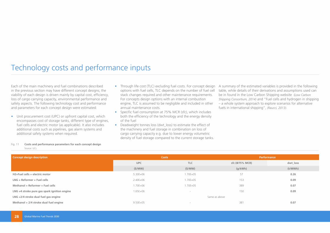
Each of the main machinery and fuel combinations described in the previous section may have different concept designs; the viability of each design is driven mainly by capital cost, efficiency, loss of cargo carrying capacity, environmental performance and safety aspects. The following technology cost and performance and parameters for each concept design were estimated:

• Unit procurement cost (UPC) or upfront capital cost, which encompasses cost of storage tanks, different type of engines, fuel cells and electric motor (as applicable). It also includes additional costs such as pipelines, gas alarm systems and additional safety systems when required.

• Through life cost (TLC) excluding fuel costs. For concept design options with fuel cells, TLC depends on the number of fuel cell stack changes required and other maintenance requirements. For concepts design options with an internal combustion engine, TLC is assumed to be negligible and included in other annual maintenance costs.

• Specific fuel consumption at 75% MCR (sfc), which includes both the efficiency of the technology and the energy density of the fuel

• Deadweight tonnes loss (dwt_loss) to estimate the effect of the machinery and fuel storage in combination on loss of cargo carrying capacity e.g. due to lower energy volumetric density of fuel storage compared to the current storage tanks.

A summary of the estimated variables is provided in the following table, while details of their derivations and assumptions used can be in found in the Low Carbon Shipping website (Low Carbon Shipping Consortium, 2014) and “Fuel cells and hydrogen in shipping – a whole system approach to explore scenarios for alternative fuels in international shipping”, (Raucci, 2013).

Technology costs and performance inputs

Fig. 11 Costs and performance parameters for each concept design Source: UCL

Concept design description Costs Performance

UPC TLC sfc (@75% MCR) dwt_loss

($/MW) ($/MW) (g/kWh) (t/MWh)

H2+Fuel cells + electric motor 5.30E+06 1.70E+05 57 0.26

LnG + Reformer + Fuel cells 2.40E+06 1.70E+05 153 0.09

Methanol + Reformer + Fuel cells 1.70E+06 1.70E+05 389 0.07

LnG +4 stroke pure gas spark ignition engine 1.65E+06 - 150 0.09

LnG +2/4 stroke dual fuel gas engine Same as above

Methanol + 2/4 stroke dual fuel engine 9.50E+05 - 381 0.07


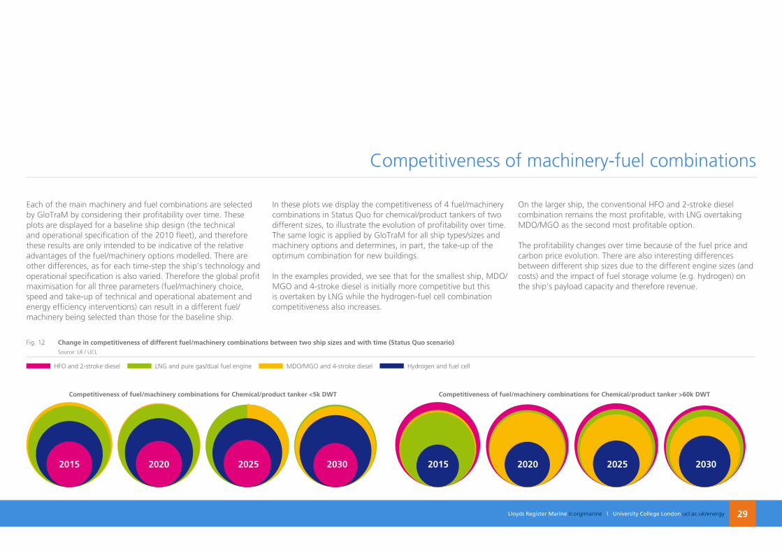
Each of the main machinery and fuel combinations are selected by GloTraM by considering their profitability over time. These plots are displayed for a baseline ship design (the technical and operational specification of the 2010 fleet), and therefore these results are only intended to be indicative of the relative advantages of the fuel/machinery options modelled. There are other differences, as for each time-step the ship’s technology and operational specification is also varied. Therefore the global profit maximisation for all three parameters (fuel/machinery choice, speed and take-up of technical and operational abatement and energy efficiency interventions) can result in a different fuel/machinery being selected than those for the baseline ship.

In these plots we display the competitiveness of 4 fuel/machinery combinations in Status Quo for chemical/product tankers of two different sizes, to illustrate the evolution of profitability over time. The same logic is applied by GloTraM for all ship types/sizes and machinery options and determines, in part, the take-up of the optimum combination for new buildings.

In the examples provided, we see that for the smallest ship, MDO/MGO and 4-stroke diesel is initially more competitive but this is overtaken by LNG while the hydrogen-fuel cell combination competitiveness also increases.

On the larger ship, the conventional HFO and 2-stroke diesel combination remains the most profitable, with LNG overtaking MDO/MGO as the second most profitable option.

The profitability changes over time because of the fuel price and carbon price evolution. There are also interesting differences between different ship sizes due to the different engine sizes (and costs) and the impact of fuel storage volume (e.g. hydrogen) on the ship’s payload capacity and therefore revenue.

Competitiveness of machinery-fuel combinations

Fig. 12 Change in competitiveness of different fuel/machinery combinations between two ship sizes and with time (Status Quo scenario) Source: LR / UCL

Competitiveness of fuel/machinery combinations for Chemical/product tanker <5k DWT Competitiveness of fuel/machinery combinations for Chemical/product tanker >60k DWT

HFO and 2-stroke diesel LNG and pure gas/dual fuel engine MDO/MGO and 4-stroke diesel Hydrogen and fuel cell

2015 20152020 20202025 20252030 2030


Marine fuel mix 2030


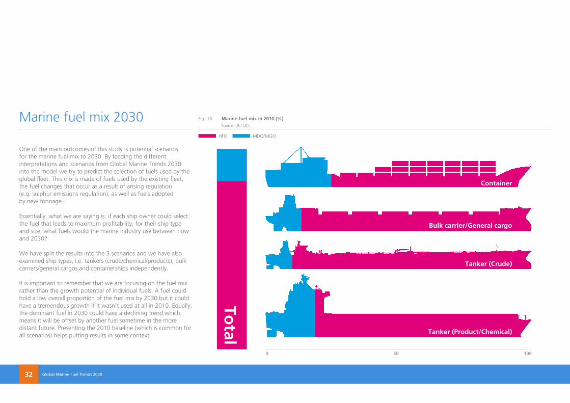
One of the main outcomes of this study is potential scenarios for the marine fuel mix to 2030. By feeding the different interpretations and scenarios from Global Marine Trends 2030 into the model we try to predict the selection of fuels used by the global fleet. This mix is made of fuels used by the existing fleet, the fuel changes that occur as a result of arising regulation (e.g. sulphur emissions regulation), as well as fuels adopted by new tonnage.

Essentially, what we are saying is: if each ship owner could select the fuel that leads to maximum profitability, for their ship type and size, what fuels would the marine industry use between now and 2030?

We have split the results into the 3 scenarios and we have also examined ship types, i.e. tankers (crude/chemical/products), bulk carriers/general cargos and containerships independently.

It is important to remember that we are focusing on the fuel mix rather than the growth potential of individual fuels. A fuel could hold a low overall proportion of the fuel mix by 2030 but it could have a tremendous growth if it wasn’t used at all in 2010. Equally, the dominant fuel in 2030 could have a declining trend which means it will be offset by another fuel sometime in the more distant future. Presenting the 2010 baseline (which is common for all scenarios) helps putting results in some context:

Marine fuel mix 2030 Fig. 13 Marine fuel mix in 2010 (%) Source: LR / UCL

HFO MDO/MGO

Container

Bulk carrier/General cargo

Tanker (Crude)

Tanker (Product/Chemical)

0 10050

Total


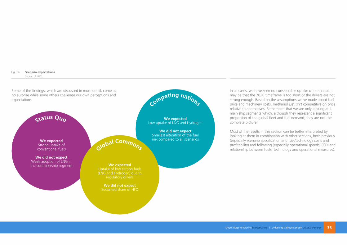
Some of the findings, which are discussed in more detail, come as no surprise while some others challenge our own perceptions and expectations:

In all cases, we have seen no considerable uptake of methanol. It may be that the 2030 timeframe is too short or the drivers are not strong enough. Based on the assumptions we’ve made about fuel price and machinery costs, methanol just isn’t competitive on price relative to alternatives. Remember, that we are only looking at 4 main ship segments which, although they represent a significant proportion of the global fleet and fuel demand, they are not the complete picture.

Most of the results in this section can be better interpreted by looking at them in combination with other sections, both previous (especially scenario specification and fuel/technology costs and profitability) and following (especially operational speeds, EEDI and relationship between fuels, technology and operational measures).

Fig. 14 Scenario expectations Source: LR / UCL

We expectedLow uptake of LNG and Hydrogen

We did not expectSmallest alteration of the fuel mix compared to all scenarios

Competing nations

We expectedStrong uptake of conventional fuels

We did not expectWeak adoption of LNG in the containership segment

Status Quo

We expectedUptake of low carbon fuels (LNG and Hydrogen) due to

regulatory drivers

We did not expectSustained share of HFO

Global Commons


HFO MDO/MGO LSHFO LNG Hydrogen Methanol


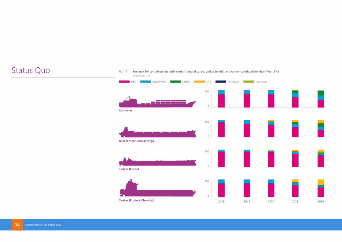
Status Quo Fig. 15 Fuel mix for containership, bulk carrier/general cargo, tanker (crude) and tanker (product/chemical) fleet (%) Source: LR / UCL

0

0

0

0

100

100

100

100

Container


Tanker (Crude)

Tanker (Product/Chemical) 2010 2015 2020 2025 2030


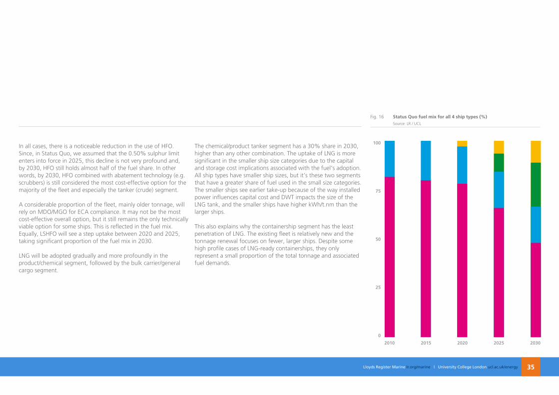
In all cases, there is a noticeable reduction in the use of HFO. Since, in Status Quo, we assumed that the 0.50% sulphur limit enters into force in 2025, this decline is not very profound and, by 2030, HFO still holds almost half of the fuel share. In other words, by 2030, HFO combined with abatement technology (e.g. scrubbers) is still considered the most cost-effective option for the majority of the fleet and especially the tanker (crude) segment.

A considerable proportion of the fleet, mainly older tonnage, will rely on MDO/MGO for ECA compliance. It may not be the most cost-effective overall option, but it still remains the only technically viable option for some ships. This is reflected in the fuel mix. Equally, LSHFO will see a step uptake between 2020 and 2025, taking significant proportion of the fuel mix in 2030.

LNG will be adopted gradually and more profoundly in the product/chemical segment, followed by the bulk carrier/general cargo segment.

The chemical/product tanker segment has a 30% share in 2030, higher than any other combination. The uptake of LNG is more significant in the smaller ship size categories due to the capital and storage cost implications associated with the fuel’s adoption. All ship types have smaller ship sizes, but it’s these two segments that have a greater share of fuel used in the small size categories. The smaller ships see earlier take-up because of the way installed power influences capital cost and DWT impacts the size of the LNG tank, and the smaller ships have higher kWh/t.nm than the larger ships.

This also explains why the containership segment has the least penetration of LNG. The existing fleet is relatively new and the tonnage renewal focuses on fewer, larger ships. Despite some high profile cases of LNG-ready containerships, they only represent a small proportion of the total tonnage and associated fuel demands.


Fig. 16 Status Quo fuel mix for all 4 ship types (%) Source: LR / UCL

2010

0

50

100

75

25

2015 2020 2025 2030


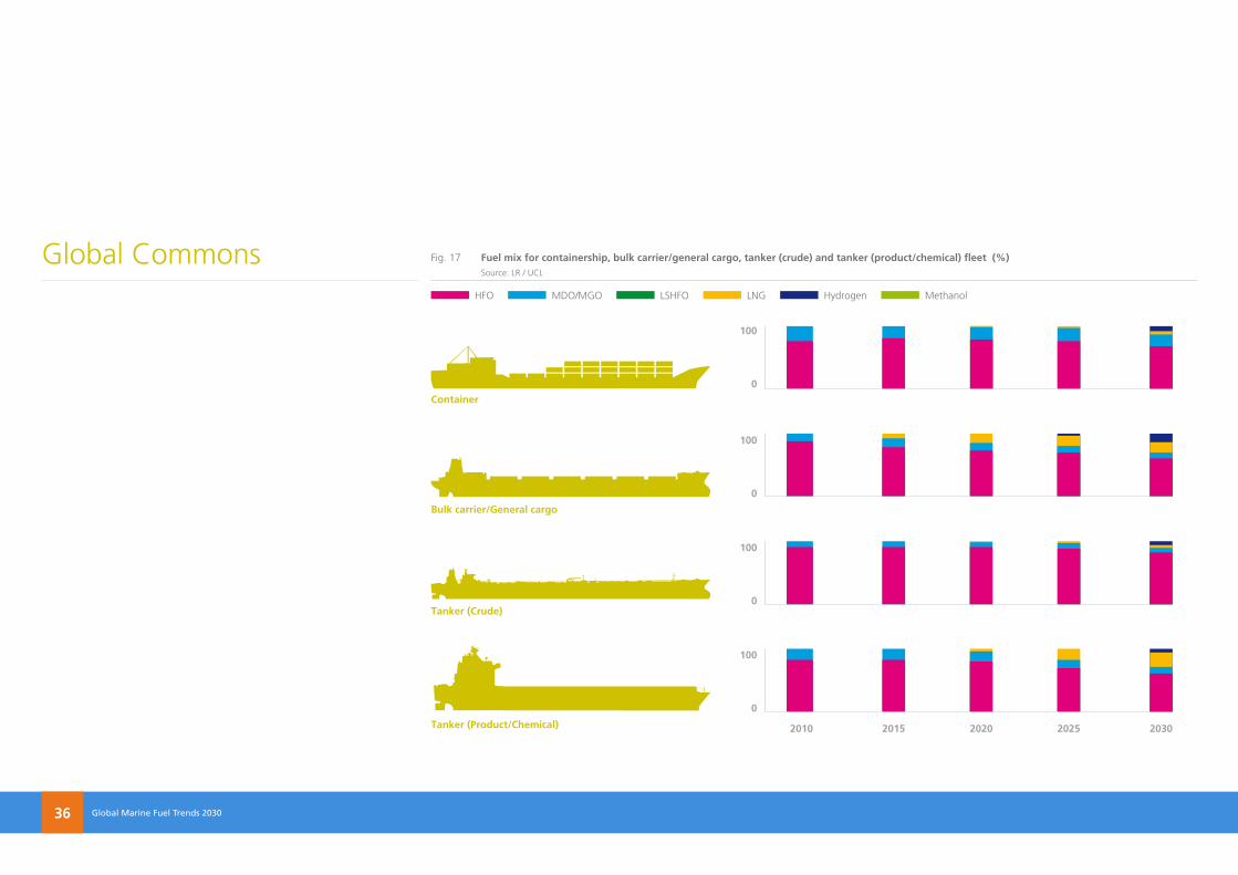
Global Commons Fig. 17 Fuel mix for containership, bulk carrier/general cargo, tanker (crude) and tanker (product/chemical) fleet (%) Source: LR / UCL


0

0

0

0

100

100

100

100

Container


Tanker (Crude)

Tanker (Product/Chemical) 2010 2015 2020 2025 2030


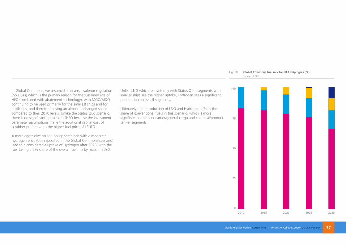
In Global Commons, we assumed a universal sulphur regulation (no ECAs) which is the primary reason for the sustained use of HFO (combined with abatement technology), with MGO/MDO continuing to be used primarily for the smallest ships and for auxiliaries, and therefore having an almost unchanged share compared to their 2010 levels. Unlike the Status Quo scenario, there is no significant uptake of LSHFO because the investment parameter assumptions make the additional capital cost of scrubber preferable to the higher fuel price of LSHFO.

A more aggressive carbon policy combined with a moderate hydrogen price (both specified in the Global Commons scenario) lead to a considerable uptake of Hydrogen after 2025, with the fuel taking a 9% share of the overall fuel mix by mass in 2030.

Unlike LNG which, consistently with Status Quo, segments with smaller ships see the higher uptake, Hydrogen sees a significant penetration across all segments.

Ultimately, the introduction of LNG and Hydrogen offsets the share of conventional fuels in this scenario, which is more significant in the bulk carrier/general cargo and chemical/product tanker segments.

Fig. 18 Global Commons fuel mix for all 4 ship types (%) Source: LR / UCL

2010

0

50

100

75

25

2015 2020 2025 2030


2010 2015 2020 2025 2030


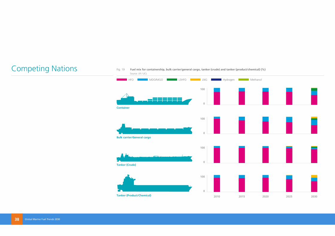
Competing Nations Fig. 19 Fuel mix for containership, bulk carrier/general cargo, tanker (crude) and tanker (product/chemical) (%) Source: LR / UCL


Container


Tanker (Crude)


0

0

0

0

100

100

100

100


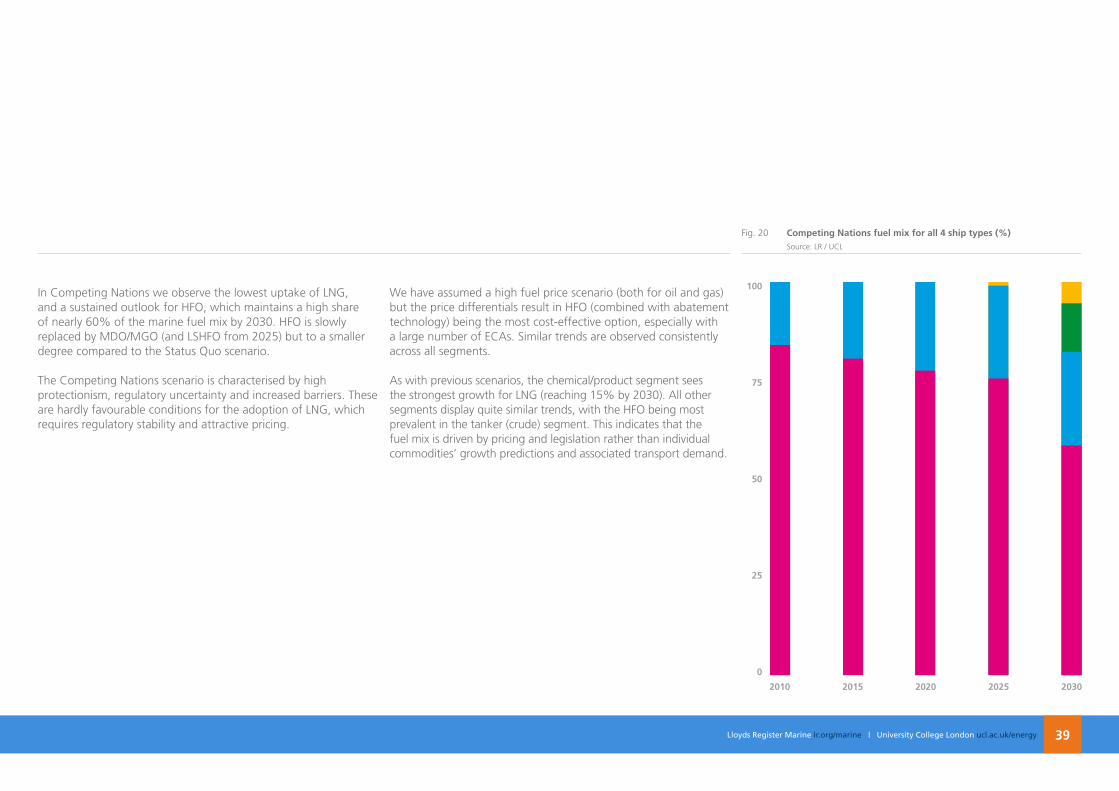
In Competing Nations we observe the lowest uptake of LNG, and a sustained outlook for HFO, which maintains a high share of nearly 60% of the marine fuel mix by 2030. HFO is slowly replaced by MDO/MGO (and LSHFO from 2025) but to a smaller degree compared to the Status Quo scenario.

The Competing Nations scenario is characterised by high protectionism, regulatory uncertainty and increased barriers. These are hardly favourable conditions for the adoption of LNG, which requires regulatory stability and attractive pricing.

We have assumed a high fuel price scenario (both for oil and gas) but the price differentials result in HFO (combined with abatement technology) being the most cost-effective option, especially with a large number of ECAs. Similar trends are observed consistently across all segments.

As with previous scenarios, the chemical/product segment sees the strongest growth for LNG (reaching 15% by 2030). All other segments display quite similar trends, with the HFO being most prevalent in the tanker (crude) segment. This indicates that the fuel mix is driven by pricing and legislation rather than individual commodities’ growth predictions and associated transport demand.

Fig. 20 Competing nations fuel mix for all 4 ship types (%) Source: LR / UCL

2010

0

50

100

75

25

2015 2020 2025 2030


EEDI and design vs. operational speeds


All else being equal, different fuel, machinery and technology combinations can result in a different ‘optimum’ speed. Both in reality and in GloTraM, variations in the specification of ship’s technical and operational parameters are observed between different ship sizes within each segment. Typically, higher fuel and carbon costs will drive lower speeds. However, in practice there is an interaction with the technical efficiency of the ship. In a given market, ships with better technical efficiency, expressed in terms of EEDI, can maximise their profit by operating at higher speeds than less efficient ships.

In the GloTraM output, differences between design and operational speeds can be explained due to the fact that the design speed is selected using the fuel price and market conditions specific to the time-step at which the ship enters the market, whereas the operational speed is updated as the fuel price and market conditions and technical specification (e.g. due to retrofit of energy efficiency technology) vary with time.

In all cases, newbuild ships entering the fleet will comply with the relevant design efficiency requirements (EEDI) over time, for the given ship type and size. These are known today and become more onerous within a defined timeframe (in all scenarios 10%, 20% and 30% improvement by 2015, 2020 and 2025 respectively).

The regulation only sets a minimum compliance requirement.However, fuel change (to lower carbon factor), design speed reductions or technology uptake may result in an EEDI lower than regulated, which also happens to be profitable at a given time-step. In this case, this is selected as the newbuild ship’s specification.

Consequently, in some cases, the EEDI trend of the newbuild ships may increase over time, for example because the specific price, market and regulation backdrop in a later time-step finds a profit maximising solution that remains compliant with the minimum EEDI regulation but results in a higher emissions intensity. This does not mean non-compliance (EEDI will still be at least equal to the regulatory level).

It should be emphasised that the EEDI parameter is just a means to look at the evolving technical specification of the fleet. The actual energy demands and emissions of the fleet are a function of operational parameters, and as operational speeds depart significantly from design speeds EEDI will become increasingly misrepresentative (this is often observed in the scenario results, with older less technologically advanced ships operating at lower speeds to remain competitive in an environment of higher fuel prices).

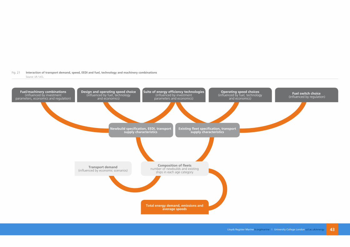
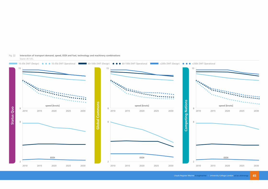
It may help if we tried to visualise the complex interactions between transport demand, speed, EEDI and fuel, technology and machinery combinations:



Composition of fleetsnumber of newbuilds and existing

ships in each age category

Transport demand(influenced by economic scenarios)

Total energy demand, emissions and average speeds

newbuild specification, EEDI, transport supply characteristics

Existing fleet specification, transport supply characteristics

Fuel/machinery combinations (influenced by investment

parameters, economics and regulation)

Design and operating speed choice (influenced by fuel, technology

and economics)

Suite of energy efficiency technologies (influenced by investment

parameters and economics)

operating speed choices (influenced by fuel, technology

and economics)

Fuel switch choice (influenced by regulation)

Fig. 21 Interaction of transport demand, speed, EEDI and fuel, technology and machinery combinations Source: LR / UCL


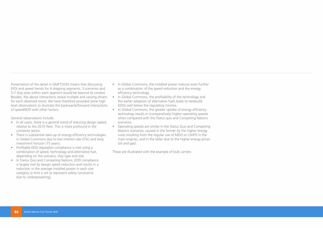
Presentation of the detail in GMFT2030 means that discussing EEDI and speed trends for 4 shipping segments, 3 scenarios and 5-7 ship sizes within each segment would be beyond its context. Besides, the above interactions reveal multiple and varying drivers for each observed trend. We have therefore provided some high level observations to illustrate the backwards/forward interactions of speed/EEDI with other factors.

General observations include:• In all cases, there is a general trend of reducing design speed,

relative to the 2010 fleet. This is more profound in the container sector.

• There is substantial take-up of energy efficiency technologies in Global Commons due to low interest rate (5%) and long investment horizon (15 years).

• Profitable EEDI regulation compliance is met using a combination of speed, technology and alternative fuel, depending on the scenario, ship type and size.

• In Status Quo and Competing Nations, EEDI compliance is largely met by design speed reduction and results in a reduction in the average installed power in each size category (a limit is set to represent safety constraints due to underpowering).

• In Global Commons, the installed power reduces even further as a combination of the speed reduction and the energy efficiency technology.

• In Global Commons, the profitability of the technology and the earlier adoption of alternative fuels leads to newbuild EEDIs well below the regulatory minima.

• In Global Commons, the greater uptake of energy efficiency technology results in (comparatively) higher operating speeds when compared with the Status quo and Competing Nations scenarios.

• Operating speeds are similar in the Status Quo and Competing Nations scenarios, caused in the former by the higher energy costs resulting from the regular use of MDO or LSHFO in the main engines, and in the latter due to the higher energy prices (oil and gas).

These are illustrated with the example of bulk carriers


Fig. 22 Interaction of transport demand, speed, EEDI and fuel, technology and machinery combinations Source: LR / UCL

15 1515

8 88

8 88

2 22

2010 20102010

2010 20102010

2015 20152015

2015 20152015

2020 20202020

2020 20202020

2025 20252025

2025 20252025

2030 20302030

2030 20302030

Co

mp

etin

g n

atio

ns

Stat

us

Qu

o

Glo

bal

Co

mm

on

s

10-35k DWT (Design) 10-35k DWT Operational 60-100k DWT (Design) 60-100k DWT Operational >200k DWT (Design) >200k DWT Operational

speed [knots] speed [knots]speed [knots]

EEDI EEDIEEDI


Marine fuel demand 2030


20302010 2015 2020 2025


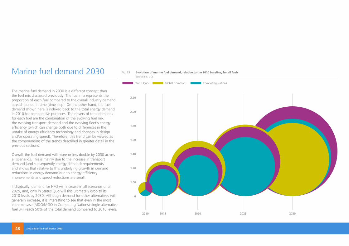
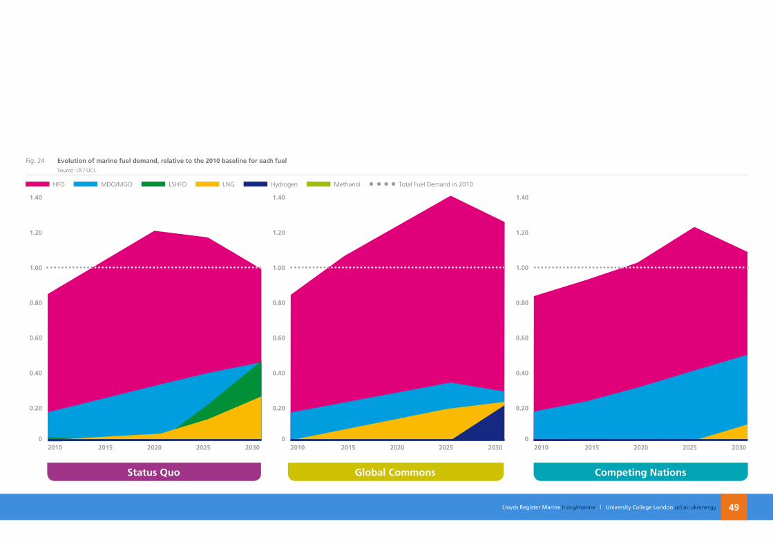
The marine fuel demand in 2030 is a different concept than the fuel mix discussed previously. The fuel mix represents the proportion of each fuel compared to the overall industry demand at each period in time (time step). On the other hand, the fuel demand shown here is indexed back to the total energy demand in 2010 for comparative purposes. The drivers of total demands for each fuel are the combination of the evolving fuel mix, the evolving transport demand and the evolving fleet’s energy efficiency (which can change both due to differences in the uptake of energy efficiency technology and changes in design and/or operating speed). Therefore, this trend can be viewed as the compounding of the trends described in greater detail in the previous sections.

Overall, the fuel demand will more or less double by 2030 across all scenarios. This is mainly due to the increase in transport demand (and subsequently energy demand) requirements and shows that relative to this underlying growth in demand reductions in energy demand due to energy efficiency improvements and speed reductions are small.

Individually, demand for HFO will increase in all scenarios until 2025, and, only in Status Quo will this ultimately drop to its 2010 levels by 2030. Although demand for other alternatives will generally increase, it is interesting to see that even in the most extreme case (MDO/MGO in Competing Nations) single alternative fuel will reach 50% of the total demand compared to 2010 levels.


0

1.00

1.80

1.60

1.40

1.20

2.20

2.00

Fig. 23 Evolution of marine fuel demand, relative to the 2010 baseline, for all fuels Source: LR / UCL



0 0

0.20 0.20

1.20 1.20

1.00 1.00

0.80 0.80

0.60 0.60

0.40 0.40

1.40 1.40

Status Quo Global Commons


Fig. 24 Evolution of marine fuel demand, relative to the 2010 baseline for each fuel Source: LR / UCL

HFO MDO/MGO LSHFO LNG Hydrogen Methanol Total Fuel Demand in 2010

201020102010 201520152015 202020202020 202520252025 2030203020300

0.20

1.20

1.00

0.80

0.60

0.40

1.40

Competing nations


Emissions 2030


In this study, CO2 emissions from the fuel combustion activities at

the point of operation are modelled through the use of carbon factors based on the carbon content of the fuels and fuel blends. Therefore the main assumption is that most of the GHG emissions come from the CO

2 released in fuel combustion activities of the

vessels during their operation. The other main assumption made in this work is that all the carbon from the fuel is converted into CO

2,

assuming that no other harming greenhouse gases arising from incomplete combustion are released.

Despite being simplistic, these assumptions can be accepted as being statistically representative, since it can be demonstrated that at present, in most cases CO

2 emissions constitute more that

99% of the GHG released in fuel combustion processes. Also, combustion is usually performed in the presence of enough excess oxygen to avoid incomplete combustion.

However, this assumption may not remain valid if alternative and bio fuels take a greater role in the shipping, accounting for emissions associated with upstream processes and for non-CO

2 emissions, for example methane slip. This could show that

fuels which, on the basis of operational emissions alone, appear attractive have significant wider impacts that need to be taken into account to enable a fair comparison and development of appropriate mitigation policies. Further work is ongoing to enable GloTraM to incorporate these wider impacts in results, taking into account “Life Cycle Assessment of Present and Future Marine Fuels “ (Bengtsson, 2011).

Emissions accounting framework


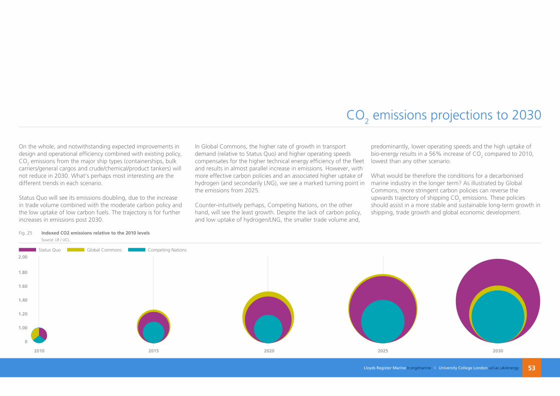
On the whole, and notwithstanding expected improvements in design and operational efficiency combined with existing policy, CO

2 emissions from the major ship types (containerships, bulk

carriers/general cargos and crude/chemical/product tankers) will not reduce in 2030. What’s perhaps most interesting are the different trends in each scenario.

Status Quo will see its emissions doubling, due to the increase in trade volume combined with the moderate carbon policy and the low uptake of low carbon fuels. The trajectory is for further increases in emissions post 2030.

In Global Commons, the higher rate of growth in transport demand (relative to Status Quo) and higher operating speeds compensates for the higher technical energy efficiency of the fleet and results in almost parallel increase in emissions. However, with more effective carbon policies and an associated higher uptake of hydrogen (and secondarily LNG), we see a marked turning point in the emissions from 2025.

Counter-intuitively perhaps, Competing Nations, on the other hand, will see the least growth. Despite the lack of carbon policy, and low uptake of hydrogen/LNG, the smaller trade volume and,

predominantly, lower operating speeds and the high uptake of bio-energy results in a 56% increase of CO

2 compared to 2010,

lowest than any other scenario.

What would be therefore the conditions for a decarbonised marine industry in the longer term? As illustrated by Global Commons, more stringent carbon policies can reverse the upwards trajectory of shipping CO

2 emissions. These policies

should assist in a more stable and sustainable long-term growth in shipping, trade growth and global economic development.

CO2 emissions projections to 2030

1.00

0

1.80

1.60

1.40

1.20

2.00


Fig. 25 Indexed Co2 emissions relative to the 2010 levels Source: LR / UCL

2010 2015 2020 2025 2030


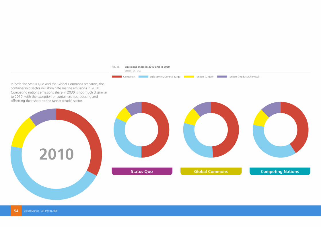
In both the Status Quo and the Global Commons scenarios, the containership sector will dominate marine emissions in 2030. Competing nations emissions share in 2030 is not much dissimilar to 2010, with the exception of containerships reducing and offsetting their share to the tanker (crude) sector.

Fig. 26 Emissions share in 2010 and in 2030 Source: LR / UCL

Containers Bulk carriers/General cargo Tankers (Crude) Tankers (Product/Chemical)

Competing nationsStatus Quo Global Commons

2010


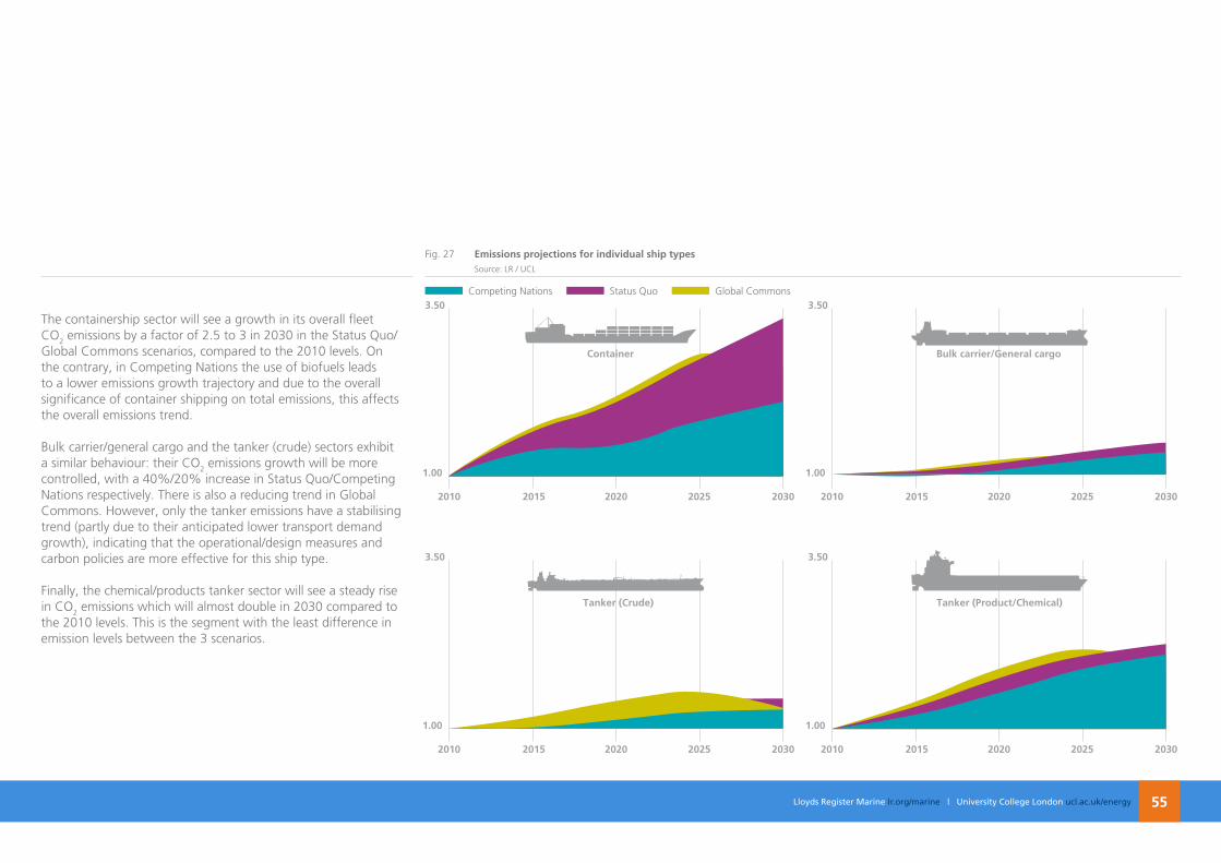
The containership sector will see a growth in its overall fleet CO

2 emissions by a factor of 2.5 to 3 in 2030 in the Status Quo/

Global Commons scenarios, compared to the 2010 levels. On the contrary, in Competing Nations the use of biofuels leads to a lower emissions growth trajectory and due to the overall significance of container shipping on total emissions, this affects the overall emissions trend.

Bulk carrier/general cargo and the tanker (crude) sectors exhibit a similar behaviour: their CO

2 emissions growth will be more

controlled, with a 40%/20% increase in Status Quo/Competing Nations respectively. There is also a reducing trend in Global Commons. However, only the tanker emissions have a stabilising trend (partly due to their anticipated lower transport demand growth), indicating that the operational/design measures and carbon policies are more effective for this ship type.

Finally, the chemical/products tanker sector will see a steady rise in CO

2 emissions which will almost double in 2030 compared to

the 2010 levels. This is the segment with the least difference in emission levels between the 3 scenarios.

Fig. 27 Emissions projections for individual ship types Source: LR / UCL


3.50

2010 2015 2020 2025 2030

1.00

3.50

2010 2015 2020 2025 2030

1.00

3.50

2010 2015 2020 2025 2030

1.00

3.50

2010 2015 2020 2025 2030

1.00

Competing Nations Status Quo Global Commons

Tanker (Crude)

Container Bulk carrier/General cargo


Forecasts are invariably proved wrong and humiliate the forecaster, and forecasting the evolution of a system as complex as the global shipping industry is a bold move. Not only are the inputs (evolution of trade, regulation, fuel price, technology) highly uncertain, but also so are the mechanisms through which these inputs interact to produce the outcomes we (will) observe. However, to shy away from this challenge seems cowardly, and means strategizing and planning could becomes whimsical and subjective. We think, if handled with care, transparently defined assumptions and models do provide a useful tool for testing out and discussing ideas and preconceptions obtained more organically e.g. from experience and judgment.

The research behind Global Marine Fuel Trends started in 2010, in the RCUK Energy programme and industry funded project Low Carbon Shipping - A Systems Approach, and has evolved through a number of overlapping projects and studies, carried out with a mixture of shipping stakeholders over the last few years and stimulated by the pressing need of the marine industry to understand the transformation referred to in the Foreword. The fact that it has taken until now to produce a major report using the shipping system model GloTraM is indicative of how much we’ve had to learn in order to build something worthy of sharing outside of our immediate research community (the academic and industry partners with whom we have collaborated to date).

One outcome of the work carried out to date is to learn more about what we do not currently know - an industry can look straightforward when you know nothing about it. The Low Carbon Shipping research community has produced much greater and wider insight than is included in this report and incorporated in GloTraM to date. Through a new project, Shipping in Changing Climates, we are fortunate to have the opportunity to continue to carry out the in-depth work, with a range of partners, that we hope will produce new insights and evidence and further iterations of this work. The aim is to be a part of an enduring, multidisciplinary and independent research community strongly linked to industry and capable of informing the policy making process and shipping’s broad mix of stakeholders as they transition to a low carbon, more resilient future.

Dr Tristan SmithLecturer in Energy and TransportUCL Energy Institute

PostScript


The GMFT2030 Team

Dimitris is a Lead Environmental Consultant at Lloyd’s Register. A naval architect, Dimitris is working closely with marine clients to develop solutions in response to environmental challenges, especially in the area of novel and emerging technologies. He was the LR project manager in GMFT2030.Dimitris Argyros

Tristan is a lecturer at UCL Energy Institute where he leads the Transport team’s shipping research activities. He has an academic and practitioner background as a naval architect, and has been working on interdisciplinary modelling and analysis of shipping for the last 4 years. He was coordinator of the project “Low Carbon Shipping” and is currently leading research activity in the project “Shipping in Changing Climates”, and the IMO 3rd GHG Study.Tristan Smith

Carlo is working as Doctoral Researcher in the Transport team at UCL Energy Institute. He has a Master degree in Energy Management Engineering and five years of professional experience in strategic consulting. His PhD at UCL focuses on the development of integrated models for evaluating hydrogen and other alternative fuels in shipping.

Carlo Raucci

Nagore has been working for more than 1 year as Research Associate in the Energy Systems modelling and Transport teams at UCL Energy Institute. Her background is Chemical Engineering and during her PhD studies at University Rovira I Virgili (Spain) she used mathematical programming techniques combined with LCA and Risk Management to build optimisation frameworks for multi-objective and uncertainty-influenced problems.nagore Sabio


AIS Automatic Identification System BAU Business as Usual CCS Carbon Capture and Storage DECC Department for Energy and Transport DWT Deadweight ECA Emissions Control Area EEDI Energy Efficiency Design Index EJ Exajoule (1018 joules) GHG Green House Gas GloTraM Global Transport Model GMFT 2030 Global Marine Fuel Trends 2030 GMT 2030 Global Marine Trends 2030 HFo Heavy Fuel Oil IFo Intermediate Fuel Oil IMo International Maritime Organisation IPCC Intergovernmental Panel on Climate Change kWh Kilowatt-hour

LCS Low Carbon Shipping LnG Liquefied Natural Gas LSHFo Low Sulphur Heavy Fuel Oil MCR Maximum Continuous Rating MDo Marine Diesel Oil MGo Marine Gas Oil MW Megawatt nGo Non Governmental Organisation noX Nitrogen Oxides PTo Power Take Off RCUK Research Councils UK SFC Specific Fuel Consumption SoX Sulphur Oxide SRES Special Report on Emissions Scenarios TLC Through Life Cost UPC Unit Procurement Cost

Acronyms


Anandarajah, G., Dessens, O. & McGlade, C., 2013. Modelling of global energy scenarios under CO2 emissions pathways with TIAM-UCLLondon: UCL Energy Institute.

Bengtsson, S., 2011.Life Cycle Assessment of Present and Future Marine Fuels (Thesis)Göteborg: Chalmers University of Technology.

Buhaug, Ø. et al., 2009. Second IMO GHG studyLondon: International Maritime Organization (IMO).

Enviromental Protection Agency (EPA), November. Global trade and fuels assessment – future trends and effects of requiring clean fuels in the marine sector. [Online] Available at: www.epa.gov/nonroad/marine/ci/420r08021.pdf[Accessed 10 January 2013].

IEA, 2011. Technology roadmap. Biofuels for TransportParis: OECD/IEA.Low Carbon Shipping Consortium, 2014. Low Carbon Shipping & Shipping in Changing Climates. [Online] Available at: www.lowcarbonshipping.co.uk/[Accessed 22 January 2014].

QinetiQ, Lloyd’s Register, University of Strathclyde, 2013. Global Marine Trends 2030 London: Fourtwentyseven.

Raucci, C., Smith, T., Argyros, D. & Sabio, N., 2013. Evaluating scenarios for alternative fuels in international shipping. London, The Energy Institute UCL and Lloyd’s Register.

Raucci, C., Smith, T., Sabio, N. & Argyros, D., 2013. Alternative fuels for international shippingLondon: UCL.

Smith, T., O’ Keefe, E., Aldous, L. & Agnolucci, P., 2013d. Assessment of Shipping’s Efficiency Using Satellite AIS data London: UCL Energy Institute.

Smith, T., O’Keefe, E., Aldous, L. & Agnolucci, P., 2013c. Assessment of shipping’s efficiency using Satellite AIS data. London, UCL Energy Institute.

Smith, T., O’Keefe, E. & Haji, S., 2013a. GloTraM method. London, UCL.

Smith, T., O’Keefe, E., Haji, S. & Agnolucci, P., 2013b. GloTraM external factorsLondon, UCL.

The Department of Energy & Climate Change, 2012. DECC fossil fuel price projections: summary. [Online] Available at: www.gov.uk/government/uploads/system/uploads/attachment_data/file/65698/6658-decc-fossil-fuel-price-projections.pdf[Accessed 10 January 2013].

UCL Energy Institute, 2013. GloTraM. [Online] Available at: www.ucl.ac.uk/energy-models/models/glotram[Accessed 10 January 2013].

References

Global Marine Fuel Trends 2030

Lloyd’s Register Group Limited71 Fenchurch StreetLondon EC3M 4BS

Tel: +44 (0)20 7423 2475E-mail: [email protected]

lr.org/marine

@LR_Marine /LloydsRegister

UCL Energy InstituteCentral House, 14 Upper Woburn Place London WC1H 0NN

Tel: +44 (0) 20 3108 5906E-mail: [email protected]

ucl.ac.uk/energy

@ucl_energy

© 2014 Lloyd’s Register and University College London. All rights reserved. No part of this publication may be reproduced or transmitted in any form or by any means, including photocopying and recording, or by any information storage and retrieval system.

Design by: Fourtwentyseven www.0427.co.uk

Global Marine Fuel Trends 2030 - LRQA · Lloyds Register Marine lr.org/marine | University College...

Documents

Transcript of Global Marine Fuel Trends 2030 - LRQA · Lloyds Register Marine lr.org/marine | University College...