Global Inflation Dynamics in the Post-Crisis Period: What ... · Global Inflation Dynamics in the...
52
Working Paper/Document de travail 2014-36 Global Inflation Dynamics in the Post-Crisis Period: What Explains the Twin Puzzle? by Christian Friedrich
Transcript of Global Inflation Dynamics in the Post-Crisis Period: What ... · Global Inflation Dynamics in the...

Working Paper/Document de travail 2014-36
Global Inflation Dynamics in the Post-Crisis Period: What Explains the Twin Puzzle?
by Christian Friedrich

2
Bank of Canada Working Paper 2014-36
August 2014
Global Inflation Dynamics in the Post-Crisis Period: What Explains the Twin Puzzle?
by
Christian Friedrich
International Economic Analysis Department Bank of Canada
Ottawa, Ontario, Canada K1A 0G9 [email protected]
Bank of Canada working papers are theoretical or empirical works-in-progress on subjects in economics and finance. The views expressed in this paper are those of the author.
No responsibility for them should be attributed to the Bank of Canada.
ISSN 1701-9397 © 2014 Bank of Canada

ii
Acknowledgements
I would like to thank, without implicating, Michael Ehrmann, Benoit Mojon, Filippo Ferroni, Robert Lavigne, Rose Cunningham, Mark Kruger, Michael Francis, Danilo Leiva-Leon for valuable comments on the paper and Bryce Shelton for excellent assistance in the data collection process. I would also like to thank all seminar participants at the Banque de France, the Bank of Canada, the Graduate Institute Geneva and all conference participants at the 6th NAFTA Central Banks Conference on the North American Economy: Outlook and Challenges for Economic Policy.

iii
Abstract
Inflation dynamics in advanced countries have produced two consecutive puzzles during the years after the global financial crisis. The first puzzle emerged when inflation rates over the period 2009–11 were consistently higher than expected, although economic slack in advanced countries reached its highest level in recent history. The second puzzle – still present today – was initially observed in 2012, when inflation rates in advanced countries were weakening rapidly despite the ongoing economic recovery. This paper specifies a global Phillips curve for headline inflation using inflation expectations by professional forecasters and a measure of economic slack at the global level over the period 1995q1–2013q3. Phillips curve data points in the period after the global financial crisis show a significantly different but consistent pattern compared to data points in the period before or during the crisis. In the next step, potential explanatory variables at the global level are assessed regarding their ability to improve the in-sample fit of the global Phillips curve. The analysis yields three main findings. First, the standard determinants can still explain a sizable share of global inflation dynamics. Second, household inflation expectations are an important addition to the global Phillips curve. And third, the fiscal policy stance helps explain global inflation dynamics. When taking all three findings into account, it is possible to closely replicate global inflation dynamics over the post-crisis period.
JEL classification: E31, E5, F41 Bank classification: Inflation and prices; International topics; Fiscal policy
Résumé
La dynamique de l’inflation au sein des pays avancés a donné lieu à deux énigmes, qui se sont succédé après la crise financière mondiale. La première apparaît au moment où, de 2009 à 2011, les taux d’inflation étaient systématiquement plus élevés que prévu tandis que le niveau des capacités excédentaires atteignait, de mémoire récente, un sommet. La seconde énigme persiste à ce jour : malgré la reprise, l’inflation connaît un affaiblissement rapide pour la première fois en 2012. Dans son étude, l’auteur spécifie tout d’abord une courbe de Phillips mondiale de l’inflation nominale en s’appuyant sur les anticipations d’inflation de prévisionnistes professionnels, ainsi qu’une mesure des capacités excédentaires à l’échelle internationale pour la période allant du 1er trimestre 1995 au 3e trimestre 2013. Après la crise, les points de données de la courbe présentent une forme homogène sensiblement différente de la forme épousée avant ou pendant la crise. L’auteur évalue ensuite l’aptitude de plusieurs variables explicatives à améliorer l’adéquation statistique sur l’échantillon pour la spécification choisie de la courbe de Phillips. De son analyse se dégagent trois conclusions importantes. 1) Les déterminants habituels permettent encore d’interpréter une bonne partie de la dynamique de l’inflation à l’échelle internationale. 2) Les anticipations d’inflation des ménages sont un apport important à la courbe de Phillips mondiale. 3) L’orientation de la politique

iv
budgétaire aide à expliquer le comportement de l’inflation dans le monde. La prise en compte de ces trois observations rend possible une reproduction plus fidèle de la dynamique de l’inflation dans l’après-crise.
Classification JEL : E31, E5, F41 Classification de la Banque : Inflation et prix; Questions internationales; Politique budgétaire

1 Introduction
Inflation dynamics in advanced countries have been largely puzzling over the recent past. While
inflation rates fell sharply during the global financial crisis and thus behaved as expected, their
subsequent post-crisis evolution is much harder to align with economic theory. In fact, two
distinct puzzles have emerged. The first puzzle is defined by the observation that inflation rates
over the period 2009-2011 were consistently higher than expected, even though economic slack
in advanced countries was at its highest level in recent history. The second puzzle emerged from
2012 onwards, when inflation rates in many advanced countries were weakening rapidly despite
the ongoing economic recovery.
The first puzzle was initially raised by Williams (2010) in the context of the United States
and later expanded to advanced countries in general by WEO (2013). The puzzle concerns
the fact that inflation rates have remained very stable following the financial crisis – despite
rising levels of unemployment. The key explanatory factors cited in WEO (2013) were stable
inflation expectations arising from successfully established inflation-targeting regimes and a
long-term decline in the slope of the Phillips curve, i.e., an increasingly weaker sensitivity of
inflation to economic slack. The main conclusion of the analysis was that as long as central
bank independence was maintained, inflation would evolve around the inflation target.
The second puzzle emerged more recently. During 2012, inflation rates in advanced coun-
tries suddenly started falling and have remained substantially below target since. In light of
these developments, the IMF has recently issued a warning about the risk of global deflation.1
Although most advanced economies still face substantial amounts of economic slack (especially
in Europe), it is specifically puzzling why the phenomenon of falling inflation rates occurs at a
time when economic slack in many countries is dissipating gradually.
In this paper, I contribute to the literature by reconciling the two puzzles at the international
level and examining a broad set of common explanations for both. I start with the specifica-
tion of a global Phillips curve that explains the dynamics of headline inflation using inflation
expectations and a measure of economic slack at the global level over the 1995q1-2013q3 period.
It turns out that all the Phillips curve data points during the post-crisis period, defined as the
time after 2009q4, show a consistent but significantly different pattern than data points before
or during the crisis period. In the next step, a variety of potential explanatory variables are
assessed in terms of their ability to improve the in-sample fit of the Phillips curve. The analysis
yields three main findings. First, the standard determinants can explain a sizable share of global
inflation dynamics. Second, household inflation expectations are an important addition to the
global Phillips curve. Moreover, household inflation expectations appear to be more volatile
than inflation expectations by professional forecasters and most likely are a proxy for energy
and food price dynamics. And third, the government budget balance helps predict inflation dy-
namics as well. When all three findings are taken into account, it is possible to closely replicate
global inflation dynamics over the post-crisis period.
While this paper explicitly deals with global inflation dynamics in the post-crisis period, it is
not the first one to examine global inflation. Although only a few papers specify a global Phillips
curve explicitly, there is a large body of academic literature that incorporates international
elements in domestic Phillips curves (see Eickmeier and Pijenburg (2013) and references cited
therein). The typical paper in this literature uses a standard Phillips curve framework and
augments it with international variables, such as import-price inflation and a global measure of
weighted (e.g., by GDP, Purchasing Power Parity (PPP), or trade) output gaps/unit labor costs.
1See Lagarde (2014).
2

Although several authors find a statistically significant impact of these global determinants on
domestic inflation rates, the findings are often only marginally significant and usually not very
robust to the sample selection.2
Papers that study global inflation dynamics more explicitly are Ciccarelli and Mojon (2005),
Hakkio (2009), Monacelli and Sala (2009), and Mumtaz and Surico (2012).3 The findings of this
smaller body of literature indicate that common components of industrial production, unem-
ployment rates, nominal wages, short- and long-term interest rates, the yield curve, and money
aggregates may be important determinants. Longer-term trends, such as sectoral trade open-
ness, have also been associated with the common elements of inflation. However, none of the
above papers discusses inflation dynamics in the post-crisis years.
The remainder of the paper is organized as follows. Section 2 defines the two inflation puz-
zles and characterizes global inflation dynamics. Section 3 contains the core of the paper and
consists of three subsections. The first sets up a global Phillips curve and explains that standard
determinants are not able to sufficiently account for global inflation dynamics in the post-crisis
period. A second subsection discusses a list of variables that could potentially explain the weak
post-crisis fit, and a third subsection identifies those variables from the list that yield the best
statistical fit. Section 4 then provides an interpretation of the findings and examines their ro-
bustness. Finally, Section 5 concludes.
2 Characterizing Global Inflation Dynamics
2.1 Defining the Two Inflation Puzzles
The first inflation puzzle was initially raised in the U.S. context. As pointed out in the in-
troductions of Ball and Mazumder (2011) and Gordon (2013), the first reference to a “missing
deflation puzzle” dates back to Williams (2010), who mentioned in a public speech that, “based
on the experience of past severe recessions,” he would have expected “inflation to fall by twice
as much as it has”. Subsequently, several authors took up the puzzle notion and tried to pro-
vide an empirical explanation for its occurrence – most of them used a version of the U.S.
Phillips curve as the underlying tool. Ball and Mazumder (2011) provide two modifications
of the Phillips curve. First, the authors measure core inflation with the weighted median of
consumer price inflation across industries, and second, they allow the slope of the Phillips curve
to change with the level and variance of inflation. Murphy (2014) discusses a similar line of ar-
guments and suggests that the time-varying slope of the Phillips curve is driven by sticky-price
and sticky-information approaches to price adjustments. By including a measure of uncertainty
about regional economic conditions, Murphy argues that the recent path of inflation is explained
well. A different approach is taken by Gordon (2013) who uses the “triangle model” from the
early 1980s to explain away the missing deflation puzzle for the United States. The triangle
model expresses current U.S. inflation with backward-looking inflation expectations, a measure
of economic slack to capture demand-side developments and a measure of energy-price shocks to
account for supply-side dynamics. When the model is estimated from the early 1960s to 1996,
it predicts the U.S. inflation rate in 2013q1 within 0.5 percentage points – without changing the
2In a very recent paper, Medel et al. (2014) study the information content of global inflation dynamics for theprediction of national inflation rates in 31 countries. Their findings indicate that, especially in recent years, thereis predictive content contained in the international inflation measure, but its impact on national inflation rates isvery heterogeneous.
3Table A1 in the Appendix shows a more detailed description of these papers.
3

slope of the Phillips curve over time. Gordon also argues that the predictions improve when
the (total) unemployment rate is replaced by an explicit measure for short-term unemployment.
Finally, Coibion and Gorodnichenko (2013) discuss the absence of disinflation dynamics in the
United States over the years 2009-2011. By using household inflation expectations as a measure
of inflation expectations in the Phillips curve, the authors manage to re-establish the Phillips
curve relationship for the United States since the 1960s.
The theoretical literature has also discussed potential explanations for the first puzzle. The
performance of DSGE models in describing inflation dynamics over the global financial crisis
and the early post-crisis period has been criticized by Hall (2011) and King and Watson (2012).
Del Negro et al. (2014) challenge these critiques by including financial frictions in a standard
DSGE model. The resulting model predicts a sharp contradiction in economic activity, along
with a modest and protracted decline in inflation following the period of financial stress at the
end of 2008. In addition, Gilchrist et al. (2013) provide evidence for a channel leading from firm
balance sheets to inflation dynamics. The authors demonstrate that firms with “weak” balance
sheets increase their prices significantly in order to generate required revenues, and firms with
strong balance sheets lower their prices in order to maintain their customer base. This finding
helps explain inflation dynamics in the United States during the crisis itself, as well as during the
early post-crisis period. Finally, Christiano et al. (2014) examine the dynamics of a broad set of
economic variables in the United States over the crisis and the post-crisis period. The authors
identify four shocks that can describe the features of the data well: a consumption wedge to
proxy the zero lower bound, a financial wedge to describe credit market frictions, a technology
shock that captures the decline of total factor productivity, and a government consumption
shock. The authors conclude that the fall in total factor productivity and the rise in the cost of
working capital were important factors that kept U.S. inflation high over the crisis.
The generalization of the first puzzle to the international level was then undertaken in WEO
(2013). Here, it was observed that inflation rates in advanced countries remained very stable fol-
lowing the financial crisis despite continuously rising unemployment rates. The key explanatory
factors cited were stable inflation expectations arising from successfully established inflation-
targeting regimes and a long-term decline in the slope of the Phillips curve, i.e., an increasingly
weaker sensitivity of inflation to economic slack. The main conclusion of the chapter is that as
long as central bank independence is maintained, inflation will evolve around the target.
Figure 1 documents the presence of the first puzzle for a broad set of advanced countries.
The bars indicate the deviation of quarterly headline inflation – measured on a year-on-year
basis – from the mean value of the implicit or explicit inflation target of the associated central
bank. The blue bars describe the deviation of the average inflation rate over the period 2009q4-
2011q4. It turns out that all countries, with the exception of Switzerland, Japan and Ireland,
have exhibited positive or only slightly negative deviations from the target during the first part
of the post-crisis period. Figure 1 also shows that at the beginning of the first puzzle period
(i.e., in 2009), annual real GDP growth across all sample countries amounted to 3.58%. Hence,
above-target inflation rates occurred at a time when economic growth was at its lowest level in
recent history and one would rather expect deflationary pressures to occur.
The second puzzle emerged more recently. From 2012 onwards, inflation rates in the same
set of advanced countries suddenly started falling and have remained substantially below target
since. This development is indicated by the red bars that show the deviation of average inflation
from target for the period 2012q1-2013q3. It turns out that most countries have experienced
a clearly negative deviation over the second part of the post-crisis period. Although most ad-
4

Figure 1: Illustration of the Two Puzzles
-3
-2
-1
0
1
2
3
Avg.
Dev
iatio
n of
Infla
tion
from
Targ
et
Puzzle 1: 2009q4-2011q4 Puzzle 2: 2012q1-2013q3
Note: Inflation targeters enter with the center of their target. The targets are 2% in all cases but the following ones: Australia (2.5%), Iceland (2.5%), Korea (3%), and Norway (2.5%). The average deviation is calculated for each of the two subsamples separately.
Average Annual Real GDP Growth: in 2009: -3.58 % in 2012: 0.35 %
p.p.
vanced economies still face substantial amounts of economic slack (especially in Europe), it is
specifically puzzling why the phenomenon of falling inflation rates occurs at a time when the
economic recovery had set in and economic slack is gradually dissipating in a large number of
countries. Figure 1 shows that at the beginning of the second puzzle period (i.e., in 2012), annual
real GDP growth across all sample countries amounted to 0.35%. Although highly discussed
in policy circles, this puzzle has not yet received much attention in the academic literature.
The most closely related papers are Svensson (2013) and Ferroni and Mojon (2014). Svensson
(2013) describes a similar experience for the case in Sweden, where inflation rates have been
below target since 1997. He argues that keeping inflation rates below target for an extended
period of time results in a 0.8 percentage point higher unemployment rate in Sweden over the
period 1997-2011. Ferroni and Mojon (2014) examine the predictive content of global inflation
for domestic inflation with a sample ranging until 2013. Using a variety of potential forecasting
models, the authors find that this is indeed the case. In the next step, the authors try to identify
the underlying forces at both the domestic and the global levels by specifying a VAR with sign
restrictions that identify two domestic (supply and demand) and two global shocks (commodity
prices and world demand). The authors specifically find that global supply-side factors, e.g.,
commodity prices, are most likely not the main driver of inflation dynamics after 2009. Instead,
the authors argue that falling inflation rates in 2008-2009, and during the second puzzle period,
are caused by demand shocks – with relative contributions of global and domestic shocks varying
by country and time.
Finally, to sum up the findings from the literature and the evidence from Figure 1, it can be
seen that both inflation puzzles appear in a broad set of advanced countries and seem to be even
stronger for countries other than the United States. Therefore, the next subsection combines
the information contained in national inflation rates to construct a “global” inflation rate.
5

2.2 Constructing Measures of Global Inflation
“Global” inflation dynamics in this paper are based on national inflation data from 25 advanced
countries over the period from 1995q1 to 2013q3.4 National inflation rates are obtained by
computing year-on-year growth rates of the individual Consumer Price Index (CPI) for each
country. The data are obtained from the OECD and come in quarterly frequency. Global
inflation rates are shown separately for headline and core inflation, where core inflation is defined
as headline inflation purged of food and energy prices. Largely based on Ciccarelli and Mojon
(2005), I use the following three methods to identify global inflation:
• A static factor model: The first approach here is the standard approach in the literature.
It relies on the first common factor of national inflation rates. The underlying (static)
factor model can be written as:
Xi,t = Λk,i × Fk,t + Ui,t (1)
Equation (1) expresses national inflation rates (Xi,t) in terms of a set of orthogonal vari-
ables, the common factors (Fk,t), with k = 1, 2, ...,K. I extract the resulting variable that
captures the largest common variation, the first common factor F1,t. The factor model
also produces factor loadings Λk,i, which range from 0 to 1, and quantify the importance
of the first common factor for each country. Finally, Ui,t represents the country-specific or
idiosyncratic part of the variation in Xi,t, which cannot be explained by the first common
factor. National inflation rates are standardized by subtracting their individual mean and
dividing by their standard deviation before entering the factor model.
• An unweighted average: The second approach is based on the unweighted arithmetic
mean of all national inflation rates. For comparison purposes with the factor model, the
resulting global inflation series is standardized as well.
• A PPP weighted average: Finally, the third approach is based on a weighted arith-
metic mean of national inflation rates, where the weights constitute world PPP shares
(normalized to 1 among all sample countries) obtained from the WEO database. Again,
the resulting global inflation series is standardized by subtracting the mean and dividing
by its standard deviation.
Figure 2 shows the results. The global inflation rates obtained using any of the three ap-
proaches are very similar. The following observations emerge: First, headline inflation is more
volatile than core inflation (note the different scales in the two plots), especially during the ac-
tual crisis period. Second – in line with the first puzzle – the period 2009-2011 shows a sustained
upward movement in both inflation concepts. Third – in line with the second puzzle – more
recently, all measures of global inflation show a clear downward trend.
The remainder of this paper deals with the specification of a global Phillips curve based on
global headline inflation and the factor approach as the aggregation technique.5 In order to
explain global inflation dynamics with global determinants, all potential explanatory variables
4I hereby follow the convention of the literature to use the “global” terminology but keeping the focus onadvanced countries only (see Ciccarelli and Mojon (2005) for example). The sample countries correspond tothe ones presented in Figure 1 and comprise Australia, Austria, Belgium, Canada, Denmark, Finland, France,Germany, Greece, Iceland, Ireland, Israel, Italy, Japan, Korea, Luxembourg, Netherlands, New Zealand, Norway,Portugal, Spain, Sweden, Switzerland, the United Kingdom and the United States.
5The robustness of the results to alternative aggregation techniques is examined in Section 4.2.
6

Figure 2: Global Headline (left) and Core (right) Inflation-4
-20
24
1995q1 2000q1 2005q1 2010q1 2015q1Date
Headline Inflation, 1st Factor Headline Inflation, unw. Avg.Headline Inflation, w. Avg.
-2-1
01
23
1995q1 2000q1 2005q1 2010q1 2015q1Date
Core Inflation, 1st Factor Core Inflation, unw. Avg.Core Inflation, w. Avg.
are aggregated from the national to the global level using the same methods as shown above.
However, not all potential explanatory variables are available for the full set of sample countries
and, with only a very few exceptions, I include only those national variables in the aggregation
process that cover the entire sample period.6
3 Specifying a Global Phillips Curve
The goal of this section is to specify a global Phillips curve and specifically examine the impact
of the crisis on its structure. The first subsection presents the shape of the standard Phillips
curve before, during and after the crisis and discusses the relationship between the previously
identified puzzles. The second subsection presents a large set of potential explanations for the
puzzles and introduces a strategy to test for the most likely one(s). Finally, the third subsection
discusses the outcome of the tests and specifies an augmented global Phillips curve.
3.1 The Global Phillips Curve with Standard Determinants
Following the identification of a global inflation rate in Section 2.2, this subsection aims to
explain global inflation using standard determinants from the literature. In order to specify
a global Phillips curve for global headline inflation, I largely follow the steps of Coibion and
Gorodnichenko (2013) who specify a Phillips curve in the U.S. context. First, I calculate a mea-
sure of global “surprise” inflation that is obtained by subtracting global inflation expectations
from the previously obtained global headline inflation series based on the first common factor.
The global measure of inflation expectations is derived in the exact same way and is based on
national series of inflation expectations by professional forecasters for the next calendar year,
provided by Consensus Economics. Second, as a measure of economic slack, I calculate a global
unemployment rate – again based on the first factor of national unemployment rates. Finally, I
plot both variables in a scatter plot with the inflation surprise measure on the vertical and the
measure of economic slack on the horizontal axis.
6Appendix Table A2 presents the exact country composition that underlies each of the global determinants.
7

Figure 3: The Global Phillips Curve I
1995q1
1995q2
1995q3
1995q4
1996q1
1996q2
1996q3
1996q4
1997q1
1997q2
1997q31997q4
1998q1
1998q21998q3
1998q4
1999q1
1999q2
1999q3
1999q4
2000q12000q2
2000q3
2000q4
2001q1
2001q2
2001q3
2001q4
2002q1
2002q2
2002q3
2002q4
2003q1
2003q2
2003q3
2003q4
2004q1
2004q22004q3
2004q4
2005q12005q2
2005q3
2005q42006q1
2006q2
2006q3
2006q4
2007q12007q2
2007q3
2007q4
2008q1
2008q2
2008q3
2008q4
2009q1
2009q2
2009q3
2009q4
2010q1
2010q22010q3
2010q4
2011q12011q2
2011q32011q4
2012q1
2012q2
2012q3
2012q4
2013q1
2013q2
2013q3
-2-1
01
2S
urpr
ise
Infla
tion
-2 -1 0 1 2Unemployment Rate, 1st Factor
Note: Surprise Inflation = Difference between the 1st factor of headline inflation and the 1st factor of inflation expectations byprofessional forecasters for the next calendar year.
Figure 4: The Global Phillips Curve II
1995q1
1995q2
1995q3
1995q4
1996q1
1996q2
1996q3
1996q4
1997q1
1997q2
1997q31997q4
1998q1
1998q21998q3
1998q4
1999q1
1999q2
1999q3
1999q4
2000q12000q2
2000q3
2000q4
2001q1
2001q2
2001q3
2001q4
2002q1
2002q2
2002q3
2002q4
2003q1
2003q2
2003q3
2003q4
2004q1
2004q22004q3
2004q4
2005q12005q2
2005q3
2005q42006q1
2006q2
2006q3
2006q4
2007q12007q2
2007q3
2007q4
2008q1
2008q2
2008q3
2008q4
2009q1
2009q2
2009q3
2009q4
2010q1
2010q22010q3
2010q4
2011q12011q2
2011q32011q4
2012q1
2012q2
2012q3
2012q4
2013q1
2013q2
2013q3
-2-1
01
2S
urpr
ise
Infla
tion
-2 -1 0 1 2OECD Output Gap, 1st Factor
Note: Surprise Inflation = Difference between the 1st factor of headline inflation and the 1st factor of inflation expectations byprofessional forecasters for the next calendar year.
8

Based on Figure 3, which shows the results, we can make the following observations:
• First, there is a negative long-run relationship between the two variables during the pre-
crisis period from 1995q1 to 2007q3 (blue line).
• Second, the relationship in the crisis period is fairly similar to the pre-crisis period between
2007q4 and 2009q3 (green line).
• And third, most importantly, the entire post-crisis period, 2009q4-2013q3, shows a signif-
icantly different, but consistent, pattern with a steeper slope and a higher intercept term
(red line).
The third observation in particular requires a more detailed discussion. Evidence so far has
suggested that there are two distinct puzzles at work, one with inflation rates for the period
2009-2011 that are too high and one with inflation rates from 2012 onwards that are too low.
However, Figure 3 now reveals that surprise inflation in the entire post-crisis period is consis-
tently more sensitive to changes in economic slack and consistently higher for reasons unrelated
to economic slack. Hence, the two puzzles discussed so far can be combined into a single one,
which I henceforth term the “Twin Puzzle.” Using the unemployment rate as a measure of
economic slack has the advantage that data are available at a quarterly frequency. However,
since the Phillips curve is mostly specified using an output gap, Figure 4 shows the same rela-
tionship using the output gap as the measure of economic slack. While the result confirms the
findings in Figure 3 (this time with a prior for a positive slope), the output gap measure has
a major drawback. As output gap data for most of the sample countries are available only at
annual frequency, the data have to be linearly interpolated to a quarterly frequency. Hence, the
observations align more closely around the regression lines, suggesting an even better fit.
Next, we can use the above findings to specify an econometric model for global inflation.
The starting point is a simple Phillips curve equation that corresponds to Figure 3. By moving
inflation expectations to the right-hand side and assigning the coefficient β, global headline
inflation (πt) is expressed in Equation (2) in terms of global inflation expectations (πet ), and the
global unemployment rate (unempt). Finally, εt represents an error term.
πt = α+ βπet + γunempt + εt (2)
Specification 1 in Table 1 shows the estimated coefficients of the baseline specification, and
Figure 5 illustrates the resulting in-sample fit. As already expected from observing Figure
3, the standard Phillips curve relationship – containing inflation expectations by professional
forecasters (PFC) and the unemployment rate – does not do very well in predicting inflation
during the post-crisis period. When examining Figure 5 more closely, however, it turns out
that the in-sample prediction does a fairly good job in capturing the higher-frequency dynamics
during this period. The only problem seems to be a level and a scaling difference from around
2009 onwards. Equation (3) therefore introduces a Post-Crisis Dummy (Dpct) that takes on the
value of 1 during the period 2009q4-2013q3 and 0 elsewhere:
πt = α+ βπet + γunempt + ψDpct + δπet ×Dpct + θunempt ×Dpct + εt (3)
9

Table 1: The Baseline Specification With and Without Post-Crisis Dummy
Dependent Variable:Headline InflationUnemployment Rate -0.54*** -0.64*** -0.96*** -0.95*** -0.93***
(0.00) 0 (0.00) (0.00) (0.00)Inflation Expectations by PFC, next year 0.71*** 1.00 1.01*** 1.00 0.97***
(0.00) (.) (0.00) (.) (0.00)Post-Crisis Dummy 2.99*** 2.98*** 3.32***
(0.00) (0.00) (0.00)Unemployment Rate x Post-Crisis Dummy -1.47*** -1.48*** -1.54***
(0.00) (0.00) (0.00)Infl. Exp. By PFC x Post-Crisis Dummy 0.68***
(0.00)Observations 75 75 75 75 75R-squared 0.52 0.78 0.80
Note: P-Values in parentheses. Constant not reported. The stars indicate significance levels (also in all subsequent tables): *** p<0.01, ** p<0.05, * p<0.1.
(5)(1) (2) (3) (4)
Figure 5: In-Sample Fit using the Standard Phillips Curve Relationship
-4-2
02
4
1995q1 2000q1 2005q1 2010q1 2015q1Date
Actual Inflation Baseline Specification
Note: Actual Inflation = 1st factor of headline inflation. Baseline Specification = In-sample fit for thestandard global Phillips curve specification, containing the unemployment rate and inflation expec-tations by professional forecasters.
Equation (3) is written in the most general way. By also interacting the post-crisis dummy
with all the other variables in the equation, it allows the effect of unemployment and inflation ex-
pectations to differ during the post-crisis period and thus to account for the scaling discrepancy
noted in Figure 5. Specification 5 in Table 1 indicates that inflation is more sensitive to inflation
expectations by professional forecasters and to the measure of economic slack during the post-
crisis period. However, Specifications 3 and 5 also show that the difference between adding and
excluding the interaction of the post-crisis dummy with inflation expectations is fairly small. In
addition, the in-sample prediction based on Specification 5 is presented in Figure 6. Also, it is
10

Figure 6: In-Sample Fit With a Post-Crisis Dummy
-4-2
02
4
1995q1 2000q1 2005q1 2010q1 2015q1Date
Actual Inflation Baseline with Post-Crisis Dummy
Note: Actual Inflation = 1st factor of headline inflation. Baseline Specification = In-sample fit for thestandard global Phillips curve specification, containing the unemployment rate and inflation expec-tations by professional forecasters. Post-Crisis Dummy = Level and interaction terms of a dummytaking on the value of 1 over 2009q4-2013q3.
confirmed here that adding and interacting the post-crisis dummy with the standard Phillips
curve determinants remarkably improves the in-sample fit over the post-crisis period. Finally,
Specifications 2 and 4 in Table 1 show that the results are fairly similar when constraining the
coefficient on inflation expectations, β, to be equal to 1 (as was implicitly the case in Figure
3). Especially when looking at Specification 3, it turns out that inflation expectations receive a
coefficient close to 1, even in the unconstrained case.
Before moving on and testing which variable(s) could be underlying the post-crisis dummy, it
is helpful to conduct a historical decomposition for the determinants contained in Specification
5. The contributions of the individual determinants are calculated by combining the estimated
coefficients with the values of the underlying variables at each point in time. Figure 7 shows the
result. Inflation expectations by professional forecasters played the most important role in the
second half of the 1990s. The introduction of inflation targeting made agents and, hence, also
professional forecasters revise their inflation expectations downward. On the other hand, global
inflation dynamics in the 2000s were mostly driven by contributions of the unemployment rate.
The crisis itself was then characterized by falling inflation expectations, while unemployment
had not fully reacted yet. However, this changes significantly in the post-crisis period. Whereas
inflation expectations by professional forecasters play a key role from mid-2009 to 2011, most of
the post-crisis period is driven by a different variable. The high importance of the interaction
term between the crisis dummy and the unemployment rate suggests that the effect is closely
related to economic slack – however, it could also proxy for crisis-related dynamics in other vari-
ables. Finally, Figure 7 shows that the post-crisis dummy has shifted inflation in the post-crisis
period up by a significant amount.
11

Figure 7: Contributions of Individual Determinants – Post-Crisis Dummy-6
-4-2
02
4
Post-Crisis Dummy PFC Infl. Exp.
PFC Exp. Interaction Unemp. Rate
Unemp. Interaction Constant
Residual
1995q1 2013q32000q1 2005q1 2010q1
3.2 Potential Explanatory Variables to Augment the Global Phillips Curve
The previous subsection has shown that adding a post-crisis dummy to the standard Phillips
curve specification significantly improves the fit during the entire period. The goal of this subsec-
tion is to give an economic meaning to the post-crisis dummy and to determine if it potentially
proxies for another variable. Since the crisis and the post-crisis periods brought a substantial
number of structural changes, the list of potential explanatory variables is long. In order to
structure the analysis, I group them in the following five categories: additional measures of
inflation expectations, additional measures of economic slack, policies and policy uncertainty,
commodity prices, and financial variables. Table 2 shows all candidate variables and their place-
ment into the categories.7
(i) Additional Measures of Inflation Expectations: Inflation expectations differ pri-
marily along the following two dimensions:
• forecasting entity (i.e., surveys among professional forecasters, surveys among households,
or expectations calculated from financial market data); and
• forecasting horizon (e.g., next calendar year or 1, 5, 10 years ahead). In general, we expect
that inflation expectations generated by professional forecasters over the longer term are
closer to central bank targets, and that inflation expectations by households over the short
term are more affected by current inflation rates.
7Summary statistics are shown in Table A3 in the Appendix.
12

The role of household inflation expectations is of particular interest in the context of the global
Phillips curve. Coibion and Gorodnichenko (2013) suggest that household inflation expectations
are good proxies for inflation forecasts by small firms. The authors argue that using these ex-
pectations yields a stable Phillips curve relationship for the United States and therefore solves
the first part of the post-crisis puzzle (i.e., inflation dynamics during 2009-2011). Unfortunately,
there is no internationally consistent series for inflation expectations by households. I therefore
use data from two different sources and treat each of them as separate variables.8 Expectations
by households appear to be more volatile, especially in the United States, and are also more
elevated compared with inflation expectations by professional forecasters – even more so during
the post-crisis period.
(ii) Additional Measures of Economic Slack: Owing to the annual frequency of in-
ternational output gap measures, this paper relies primarily on the unemployment rate as the
measure of economic slack in the Phillips curve. Under certain assumptions, output gaps and
unemployment gaps can be used interchangeably. However, in the presence of a jobless recovery
or prolonged periods of slack, traditionally measured output gaps may not align well with un-
employment gaps. Further, additional measures of economic slack, such as labor compensation
measures or unit labor costs, might become more important in times of crises.
(iii) Policies and Policy Uncertainty: The global financial crisis was followed by an
unprecedented amount of fiscal and monetary easing, possibly raising uncertainty.
• Fiscal Policy: In this paper, fiscal policy is represented by the variable Net Lending/Bor-
rowing of the General Government in % of GDP, henceforth referred to as the “government
budget balance.” Economic theory suggests that fiscal policy affects inflation dynamics
through the measure of economic slack. However, in the presence of a deep and prolonged
recession, this standard relationship could change, and large government budget deficits
could have an additional direct effect on inflation, over and above the unemployment
rate/output gap measure.
• Unconventional Monetary Policy: The adoption of unconventional monetary policies could
lead to price increases, not only in asset markets but also in goods markets.
• Inflation Expectation Uncertainty: Inflation expectations from professional forecasters
usually refer to the next calendar year. One could therefore expect an improvement in the
forecasts towards the end of the year.
(iv) Commodity Prices: Although the previous literature has shown that inflation expec-
tations, especially by households, are highly correlated with commodity-price dynamics (with a
lag), the additional inclusion of energy and food prices in the Phillips curve might improve the
fit – even more so when inflation expectations are focused on the long term.
(v) Financial Variables: A number of theoretical papers discuss the impact of financial
frictions (e.g., Christiano et al., 2014; Del Negro et al., 2014) and firm balance sheets (e.g.,
8Inflation expectations by U.S. households are from the Michigan Survey of Consumers and are based on thequestion: “By about what percent per year do you expect prices to go up or down, on the average, during thenext 12 months?” Inflation expectations by European households are provided by the OECD for 11 countries inour sample and are based on the question: “By comparison with the past 12 months, how do you expect thatconsumer prices will develop in the next 12 months?” Possible answers range from “increase more rapidly” to“fall” in five steps and are converted into an overall index.
13

Table 2: Description of Potential Explanatory Variables
# Category/Variable Description Source
Inflation ExpectationsBL Professional Forecasters, next
calendar yearInflation expectations by professional forecasters for the next calendar year Consensus
Economics1 Headline Inflation, backward-
lookingAverage of headline inflation during the last 4 quarters OECD, BoC
Calculations2 Core Inflation, backward-looking Average of core inflation over the last 4 quarters OECD, BoC
Calculations3 US Households, 1 year-ahead Inflation expectations by US households based on the question: "By what
percent do you expect prices to go up, on the average, during the next 12 months?"
Surveys of Consumers, Univ. of Michigan
4 US Households, 5+ years-ahead Inflation expectations by US households based on the question: "By about what percent per year do you expect prices to go up or down, on the average, during the next 5 to 10 years?"
Surveys of Consumers, Univ. of Michigan
5 European Households, 1 year-ahead
Index for inflation expectations by European households based on the question "By comparison with the past 12 months, how do you expect that consumer prices will develop in the next 12 months?" Possible answers range from "increase more rapidly" to "fall" in 5 steps.
OECD
6 Professional Forecasters, 5 calendar years from now
Inflation Expectations by Professional Forecasters in 5 Years Consensus Economics
7 Professional Forecasters, 10 calendar years from now
Inflation Expectations by Professional Forecasters in 10 Years Consensus Economics
8 Market-based, over the next 5 years
Difference between yields of inflation-indexed bonds and non-indexed bonds Bloomberg, BoC Calculations
9 Market-based, over the next 10+ years
Difference between yields of inflation-indexed bonds and non-indexed bonds Bloomberg, BoC Calculations
Measures of Economcic SlackBL Unemployment Rate The unemployment rate in percent OECD10 Output Gap Interpolated quarterly values of annual output gap estimates from the OECD OECD
11 Unemployment Gap Cyclical component of the unemployment rate, obtained using an HP filter OECD, BoC Calc.
12 Real GDP Gap Cyclical component of a real GDP index, obtained using an HP filter OECD, BoC Calc.13 Industry Production Gap Cyclical component of an industry production index, obtained using an HP
filterOECD, BoC Calc.
14 Industry Production Growth YoY growth rate of an industry production index OECD15 Unit Labor Cost Growth YoY growth rate of an index of unit labor costs OECD16 Labor Compensation Growth YoY growth rate of an index of labor compensation OECD
Policies and Policy Uncertainty17 Gov. Budget Balance General government net lending/borrowing in % of GDP, interpolated to
quarterly frequencyIMF
18 Growth of QE-Quantities Growth of QE quantities in % of GDP; in levels for Figure 7C, in growth rates for the empirical analysis.
Dahlhaus, Hess, Reza (2014)
19 Inflation Expectations Uncertainty Standard deviation across the individual mean forecasts/inflation expectations by professional forecasters in the next calendar year (first variable in the list)
Consensus Economics
Commodity Prices20 Oil Price YoY growth rate of Brent Index. Intercontinental
Exchange21 Energy Prices YoY growth rate of energy prices IMF22 Food Prices YoY growth rate of food prices IMF
Financial Variables23 Financial Market Uncertainty VIX Index Chicago Board
Options Exchange (CBOE)
24 Credit Growth YoY growth rate of credit to private non-fianncial sector in % of GDP BIS25 Stockmarket Growth YoY growth rate of the MSCI World index Bloomberg26 Real Estate Price Growth YoY growth rate of a real estate index (res. property, all dwellings) BIS
BL = Baseline Specification
14

Gilchrist et al., 2013) on output and inflation dynamics during the global financial crisis. In ad-
dition, Borio et al. (2013) have recently shown empirically that accounting for cyclical financial
variables can improve the estimation of potential output and the output gap. Hence, financial
variables could indeed be important drivers of inflation dynamics. I therefore examine the role
of stock market prices, real estate prices and private credit in helping to predict global inflation.
In addition, the VIX index is also tested, since uncertainty about financial developments could
be an important driver of global inflation dynamics.
3.3 What Explains the Twin Puzzle at the Global Level?
To better understand the shift in inflation dynamics, I begin by estimating the baseline spec-
ification, which contains the unemployment rate and inflation expectations from professional
forecasters for the next calendar year (results were shown in Specification 1 of Table 1). I then
re-estimate the model with the addition of each of the 26 potential explanatory variables listed in
Table 2 to optimally match the structural shift during the post-crisis period observed in Figure
3. The corresponding functional form for the analysis is given by Equation (4):
πt = α+ βπet + γunempt + ψV arXt + δπet × V arXt + θunempt × V arXt + εt (4)
where V arXt is the variable to be tested as a potential determinant that could be responsible
for the post-crisis level and slope shift. Hence, each candidate variable is included as it is, as an
interaction term with the unemployment rate and as an interaction term with the expectations
by professional forecasters. The resulting specifications are evaluated using the (lowest) Mean
Squared Error (MSE) for the following four intervals:9
• the entire sample period (1995q1-2013q3);
• the entire post-crisis period (2009q4-2013q3);
• the period of the first puzzle (2009q4-2011q4); and
• the period of the second puzzle (2012q1-2013q3).
Table 3 shows the results. The potential explanatory variables are ordered according to the
MSEs of their underlying specifications over the entire sample period from the lowest to the
highest.10 The variable with the lowest MSE of all the candidate variables is the measure of
inflation expectations by European households over the next 12 months (MSE of 0.50). Inter-
estingly, this variable is followed by a measure of inflation expectations by U.S. households over
the same time frame (MSE of 0.55). The variables that follow this selection in turn are the
growth rates of real estate prices (MSE of 0.56), as well as the growth rates of food and energy
prices (both have an MSE of 0.57).
9As some of the intervals are very short, the MSE is calculated without a degree of freedom adjustment. Thisoverstates the MSE in absolute terms but it does not affect its ordering as in all cases the same number of variablesis included in the regression
10In the remainder of this section, the MSE associated with each variable refers to the MSE of the underlyingspecification including this variable; i.e., the baseline specification plus the variable under examination.
15

Table 3: Potential Explanatory Variables Ordered by Mean Squared Error
Variable added 1995q1-2013q3 2009q4-2013q3 2009q4-2011q4 2012q1-2013q3Infl. Exp. European Households, 1 year-ahead 0.50 0.43 0.52 0.29Infl. Exp. US Households, 1 year-ahead 0.55 0.68 0.78 0.52Real Estate Price Growth 0.56 0.79 0.89 0.63Growth Rate of Food Prices 0.57 0.76 0.76 0.76Growth Rate of Energy Prices 0.57 0.75 0.80 0.67Real GDP Gap 0.58 0.60 0.75 0.31Industry Production Gap 0.58 0.60 0.70 0.42Growth Rate of Oil Price 0.59 0.77 0.83 0.70Government Budget Balance 0.60 0.78 0.83 0.70Unit Labor Cost Growth 0.60 0.87 1.03 0.60Infl. Exp. for Core Inflation, backward-looking 0.60 0.73 0.72 0.74Industry Production Growth 0.60 0.77 0.93 0.50Output Gap 0.60 0.90 1.04 0.66Credit Growth 0.60 0.83 1.02 0.48Stock Market Growth 0.60 0.87 1.08 0.51QE-Quantities 0.62 0.84 1.00 0.51Infl. Exp. by Professional Forecasters, 5 years from now 0.63 0.80 0.90 0.66Labor Compensation Growth 0.63 0.75 0.89 0.51Infl. Exp. by Financial Markets, over the next 5 years 0.64 0.75 0.93 0.42Infl. Exp. by US Households, 5+ years-ahead 0.64 0.73 0.89 0.44Infl. Exp. by Professional Forecasters, 10 years from now 0.64 0.83 0.98 0.59Financial Market Uncertainty 0.65 0.88 1.06 0.56Unemployment Gap 0.65 0.84 1.01 0.53Inflation Expectations Uncertainty 0.65 0.90 1.07 0.62Infl. Exp. for Headline Inflation, backward-looking 0.66 0.90 1.10 0.55Infl. Exp. by Financial Markets, over the next 10+ years 0.66 0.85 1.01 0.58
MemorandumBaseline 0.69 0.93 1.11 0.62
Table 4: Derivation of the Augmented Baseline Specification
Dependent Variable:Headline InflationUnemployment Rate -0.37*** -0.33*** -0.91*** -0.75***
(0.00) (0.00) (0.00) (0.00)Inflation Expectations by PFC, next year 0.30*** 0.34*** 0.51*** 0.47***
(0.00) (0.00) (0.00) (0.00)Inflation Expectations by HH, 12 months 0.64*** 0.58*** 0.54*** 0.49***
(0.00) (0.00) (0.00) (0.00)Unemp. Rate x Infl. Exp. by HH 0.12
(0.12)Infl. Exp. By PFC x Infl. Exp. by HH 0.07
(0.23)Budget Bal. in % of GDP -0.61*** -0.50***
(0.00) (0.00)GR of World Energy Prices 0.70***
(0.00)Observations 75 75 75 75R-squared 0.75 0.74 0.82 0.86
(1) (2) (3) (4)
Note: P-Values in Parentheses. Constant not reported.
16

When looking at the (entire) post-crisis period, the MSE-reducing effect of household infla-
tion expectations becomes even more pronounced. Over the entire post-crisis sample, inflation
expectations by European households reach an MSE of 0.43, while the next variables, two mea-
sures of economic slack, reach an MSE of 0.6. The effect clearly originates from the first part
of the post-crisis period: while European household inflation expectations have an MSE of 0.52
here, the next variable reaches an MSE of 0.70 during 2009q4 and 2011q4. U.S. household
inflation expectations show a slightly higher MSE but still score fourth highest among all the
potential explanatory variables in the entire crisis period (MSE of 0.68), as well as sixth highest
(MSE of 0.78) in the first part of the post-crisis period. European household inflation expecta-
tions still dominate the list of potential explanatory variables in the second part of the post-crisis
period (MSE of 0.29); however, the difference with respect to the next candidate variable be-
comes smaller (the real GDP gap with an MSE of 0.31). Given their high but relatively constant
trajectory, U.S. household inflation expectations over the next 12 months have a higher MSE
now and score relatively lower among all potential explanatory variables (MSE of 0.52). In-
terestingly, the measure of U.S. household inflation expectations 5 years ahead turns out to be
better during this period. It ranks fifth among all the candidate variables and reaches an MSE
of 0.44.
Specifications 1 and 2 in Table 4 present the results after European household inflation ex-
pectations have been added to the baseline specification. There are two ways in which European
household expectations can be included in the specification. First, by adding the two interac-
tion terms as originally shown in Equation (4) and represented by Specification 1. Since it turns
out that abstracting from both interaction terms yields only a marginally lower fit, the second
approach, as shown in Specification 2, is to add only the level term to the baseline specification.
Figure 8 plots the corresponding in-sample fit and indicates that there is only a small dif-
ference between the two approaches. Finally, the figure also includes actual global inflation for
comparison. Although the two models that include household expectations show a similar in-
sample fit, they are less precise around the peak of global inflation during the post-crisis period.
The next section will therefore examine whether there is another variable that can account for
the higher inflation trajectory during the period in question.
In addition to European household inflation expectations, Figure A1 in the Appendix repli-
cates the analysis for U.S. household inflation expectations – the variable that had the second-
lowest MSE in Table 3 (see Specifications 1 and 2 in Appendix Table A4 for details). As expected
from the MSE, the in-sample fit of U.S. household inflation expectations is lower. Although the
in-sample prediction mirrors the spike in inflation rates during the post-crisis period, there still
seems to be a scaling difference. In addition, U.S. household inflation expectations have re-
mained largely constant over the post-crisis period, yielding an overprediction of inflation rates
at the end of the period.
The analysis so far has shown that household inflation expectations, and especially the
measure based on household inflation expectations from 11 European countries, improve the
in-sample fit of global inflation significantly. This was the case for both the specification with
interaction terms and the specification without interaction terms. When comparing the in-
sample predictions with the global inflation series in Figure 8, however, it turned out that
the curves containing household inflation expectations have some difficulties in tracking global
inflation around its peak in mid-2011.
17

Figure 8: European Household Inflation Expectations added to the Baseline Specification
-4-2
02
4
1995q1 2000q1 2005q1 2010q1 2015q1Date
Actual Inflation Baseline with HH Exp. (Int.)
Baseline with HH Exp. (No Int.)
Note: Actual Inflation = 1st factor of headline inflation. Baseline Specification = In-sample fit for thestandard global Phillips curve specification, containing the unemployment rate and inflation expec-tations by professional forecasters. HH Exp. = 1st factor of inflation expectations by households overthe next 12 months. Int. = Interaction terms between HH Exp. and the two standard determinants.
Figure 9: Comparing the Best Specification with the Post-Crisis Dummy
-4-2
02
4
1995q1 2000q1 2005q1 2010q1 2015q1Date
Actual Inflation Augmented Baseline Specification
Baseline with Post-Crisis Dummy
Note: Actual Inflation = 1st factor of headline inflation. Augmented Baseline Specification = In-samplefit for the standard global Phillips curve specification, containing the unemployment rate and inflationexpectations by professional forecasters, plus the following three variables: household inflationexpectations, the budget balance in percent of GDP and energy price growth - all global and withoutinteractions. Post-Crisis Dummy = Level and interaction terms of a dummy taking on the value of 1over 2009q4-2013q3.
18

Table 5: Adding a Second Variable Conditional on Household Expectations
Variable added 1995q1-2013q3 2009q4-2013q3 2009q4-2011q4 2012q1-2013q3Government Budget Balance 0.42 0.27 0.32 0.20Growth Rate of Energy Prices 0.44 0.34 0.38 0.28Growth Rate of Oil Price 0.45 0.35 0.39 0.28Growth Rate of Food Prices 0.46 0.42 0.42 0.43Infl. Exp. US Households, 1 year-ahead 0.47 0.45 0.48 0.40Output Gap 0.48 0.40 0.45 0.34Infl. Exp. by Professional Forecasters, 5 years from now 0.49 0.44 0.48 0.39Inflation Expectations Uncertainty 0.49 0.40 0.48 0.27QE-Quantities 0.50 0.46 0.51 0.36Stock Market Growth 0.50 0.48 0.58 0.31Infl. Exp. by Financial Markets, over the next 5 years 0.50 0.45 0.53 0.33Unemployment Gap 0.50 0.40 0.49 0.25Real GDP Gap 0.50 0.46 0.54 0.32Financial Market Uncertainty 0.50 0.42 0.50 0.29Infl. Exp. by US Households, 5+ years-ahead 0.51 0.43 0.51 0.31Infl. Exp. by Professional Forecasters, 10 years from now 0.51 0.47 0.52 0.38Industry Production Gap 0.51 0.48 0.56 0.34Labor Compensation Growth 0.51 0.47 0.53 0.37Infl. Exp. by Financial Markets, over the next 10+ years 0.51 0.44 0.52 0.31Unit Labor Cost Growth 0.51 0.48 0.56 0.34Industry Production Growth 0.51 0.45 0.54 0.31Infl. Exp. for Headline Inflation, backward-looking 0.52 0.49 0.59 0.33Credit Growth 0.52 0.46 0.54 0.32Real Estate Price Growth 0.52 0.46 0.54 0.33Infl. Exp. for Core Inflation, backward-looking 0.52 0.45 0.52 0.36
Table 6: Adding a Third Variable Conditional on Household Expectations and the BudgetBalance
Variable added 1995q1-2013q3 2009q4-2013q3 2009q4-2011q4 2012q1-2013q3Growth Rate of Energy Prices 0.38 0.27 0.32 0.19Growth Rate of Oil Price 0.39 0.28 0.32 0.20Credit Growth 0.39 0.29 0.32 0.24Infl. Exp. for Headline Inflation, backward-looking 0.39 0.23 0.24 0.21Infl. Exp. by Professional Forecasters, 5 years from now 0.39 0.31 0.33 0.28Real Estate Price Growth 0.40 0.28 0.31 0.23Infl. Exp. for Core Inflation, backward-looking 0.40 0.28 0.32 0.23Infl. Exp. US Households, 1 year-ahead 0.40 0.27 0.30 0.21Infl. Exp. by Professional Forecasters, 10 years from now 0.41 0.28 0.30 0.26Output Gap 0.42 0.28 0.33 0.21Real GDP Gap 0.42 0.28 0.31 0.23Stock Market Growth 0.42 0.26 0.30 0.19Growth Rate of Food Prices 0.42 0.30 0.34 0.24Infl. Exp. by Financial Markets, over the next 10+ years 0.42 0.26 0.30 0.20Unemployment Gap 0.42 0.28 0.33 0.22Financial Market Uncertainty 0.42 0.25 0.29 0.20Infl. Exp. by Financial Markets, over the next 5 years 0.42 0.26 0.30 0.19Unit Labor Cost Growth 0.42 0.25 0.29 0.19QE-Quantities 0.42 0.26 0.30 0.19Labor Compensation Growth 0.42 0.28 0.34 0.19Infl. Exp. by US Households, 5+ years-ahead 0.42 0.26 0.30 0.19Inflation Expectations Uncertainty 0.42 0.28 0.33 0.20Industry Production Growth 0.42 0.26 0.31 0.19Industry Production Gap 0.42 0.27 0.32 0.20
Since this suggests that another variable may be a relevant driver of global inflation dynamics
as well, the set of candidate variables is examined a second time – this time conditional on the
baseline specification and European household inflation expectations. Since Figure 8 indicated
19

that there was only a small difference between the specifications with and without interaction
terms, the interaction terms are dropped for simplicity. Table 5 shows the results. The variable
that has the lowest MSE in all four samples is the government budget balance. While its MSE in
the full sample (0.42) is only slightly lower than for the next best variable (energy prices, MSE
of 0.44), the differences in the post-crisis period (0.27 vs. 0.34) and in its subsamples become
larger. Figure A2 in the Appendix shows the resulting in-sample fit improvement once the
government budget balance is added to the specification (for the coefficients, see Specification 3
in Table 4). Interestingly, the new setup closes the remaining gap between actual inflation and
the in-sample prediction in 2011 to a large extent.
Finally, the same exercise is repeated a third time – now conditional on the variables from the
baseline specification, European household inflation expectations and the government budget
balance. Table 6 presents the results. The variable that has the lowest MSEs in the overall
sample is energy-price growth. However, the difference in the MSE between energy-price growth
and the remaining explanatory variables becomes fairly small now (0.01 to the second variable,
oil-price growth, and 0.04 to the last one, the industry production gap). Although energy-price
growth is still among the best explanatory variables in the second part of the post-crisis period,
it is not among the variables with the lowest MSE in the first part of the post-crisis period.
This also shows up when examining the in-sample fit including energy-price growth in Figure
A2. There is only a marginal difference between the in-sample prediction for the version with
and without energy-price growth (for coefficients, see Specifications 3 and 4 in Table 4).
Altogether, the analysis has shown that there is no need to evaluate additional candidate
variables since the baseline specification plus household inflation expectations, the government
budget balance and energy-price growth are able to explain an overwhelming share of global
inflation dynamics over the period 1995q1-2013q3 and especially during the post-crisis period
2009q4-2013q3. This can also be seen in Figure 9, where the last specification is compared against
the post-crisis dummy and actual global headline inflation. As expected, all three curves align
very well – especially in the post-crisis period.
This subsection has identified a set of three variables – household inflation expectations, the
government budget balance and energy-price growth – that, once added to the baseline speci-
fication, can explain the dynamics of global headline inflation very well. However, the analysis
so far was quite agnostic about the potential channels through which these variables could work
and also about the extent to which they capture similar dynamics. The next section will examine
these questions in more detail, assess the robustness of the results and, additionally, repeat the
analysis for selected countries at the individual country level.
4 Discussion of Findings and Robustness
4.1 Discussion of Findings
The last section has delivered a set of variables that, when added to the standard Phillips
curve specification, significantly improve the in-sample prediction of global headline inflation –
especially during the post-crisis period. This section discusses the economic rationale behind
these variables and links them to the two puzzles – unexpectedly high inflation rates over the
2009-2011 period and unexpectedly low inflation rates from 2012 onwards – that were presented
in the introduction. As a starting point, Figure 10 shows the historical decomposition for the
20

extended set of determinants over time, analogously to Figure 7. The following three results
emerge:
1. The two standard determinants in the baseline specification – the unemployment rate and
inflation expectations by professional forecasters – are important determinants of global
inflation dynamics, even after additional variables are included.
2. Household inflation expectations are a key addition to the baseline specification. They
mimic the dynamics of inflation expectations by professional forecasters but are signifi-
cantly more volatile – especially during the (post)-crisis period. Conditional on household
inflation expectations, the contribution of energy-price inflation is fairly small.
3. The government budget balance helps to improve the in-sample fit of headline inflation.
Although the contribution of the budget balance is larger in the (post)-crisis period, its
impact is visible in the pre-crisis period as well.
In the remainder of this subsection, I discuss all three results in more detail.
Figure 10: Contributions of Individual Determinants – Augmented Baseline
-4-2
02
4
PFC Infl. Exp. HH Infl. Exp.
Unemp. Rate Budget Bal.
Energy Pr. Gr. Constant
Residual
1995q1 2000q1 2005q1 2010q1 2013q3
The first result suggests that the two standard determinants in Figure 10 are highly rel-
evant and confirms the earlier observation that when a post-crisis dummy (and two interaction
terms) are added to the baseline specification, the unemployment rate and inflation expectations
by professional forecasters for the next calendar year are key drivers of global inflation dynamics
over the entire sample period. It is also reassuring to see that the contributions of both variables
do not change significantly once the post-crisis dummy is removed and additional variables are
21

included in the specification. This can be seen when comparing their dynamics in Figure 7 and
Figure 10.11 Finally, I examine the importance of both standard determinants for the in-sample
fit, since one could be worried that after adding the new variables – such as household inflation
expectations, the budget balance or energy-price growth – to the specification, the standard de-
terminants could become irrelevant. However, Specifications 3 and 4 in Table A4 and Figure A3
in the Appendix show that this is not the case. Figure A3 contains the augmented baseline spec-
ification from the main text (as shown in Figure 9), as well as the same specification excluding
either one of the two standard determinants. It turns out that when either of the two standard
determinants are excluded, the in-sample prediction becomes worse. This is especially the case
at the more recent end of the sample period, where inflation dynamics would be overpredicted
otherwise.
The second result can be split up into three distinct observations. The first is that house-
hold inflation expectations are an important addition to the global Phillips curve. This finding is
highly in line with Coibion and Gorodnichenko (2013), who have shown that replacing inflation
expectations by professional forecasters with inflation expectations by households restores the
Phillips curve for the United States until at least 2011.12
Second, both inflation expectations by professional forecasters and inflation expectations by
households exhibit very similar high-frequency movements. Their correlation coefficient amounts
to 0.50 over the entire sample period and to 0.90 in the post-crisis period (see also Figure A4
in the Appendix). However, both series differ significantly in their amplitudes – with house-
hold inflation expectations being more volatile from 1999 onwards. The corresponding standard
deviations amount to 1.14 (0.51) for inflation expectations by professional forecasters (by house-
holds) over the 1995q1-1998q4 period and 0.53 (1.10) over the 1999q1-2013q3 period. This
observation also helps us to understand why the post-crisis dummy and its interactions – which
essentially increase the amplitude – are so successful in explaining global inflation dynamics
over the post-crisis period. More specifically, in Figure 7, there seems to be a mapping of the
interaction term between inflation expectations by professional forecasters and the post-crisis
dummy to the household inflation expectations variable in Figure 10 over the post-crisis period.
And third, one of the potential reasons for the higher volatility of household inflation expecta-
tions could be related to their strong dependence on volatile oil and energy prices. The literature
examining the formation of household inflation expectations has pointed out that household in-
flation expectations are highly responsive to gasoline price changes (e.g., for the United States:
Coibion and Gorodnichenko, 2013; Ehrmann et al., 2014). Figure 11 therefore plots household
inflation expectations against energy-price growth, oil-price growth and food-price growth.
Although all four series show similar high-frequency dynamics, their timing and amplitudes
differ over time. While energy and oil prices lead the expectation series by around 1 year over
most of the sample, the four series appear to be almost synchronized during the crisis period,
where household inflation expectations followed the commodity-price series with a much shorter
lag.
11Another notable feature of the two standard variables in both figures seems to be that there is a positivecorrelation at the beginning of the sample (until about 1999) and a negative correlation thereafter. Subsequently,the correlation coefficient over the period 1995q1 to 1998q4 amounts to 0.84, and takes on a value of -0.43 from1999q1-2013q3.
12There is an important difference between the results of Coibion and Gorodnichenko (2013) and this paper.Coibion and Gorodnichenko replace inflation expectations by professional forecasters with inflation expectationsby households. However, the first result in the previous paragraph has shown that inflation expectations byprofessional forecasters are still an important driver of inflation dynamics at the global level.
22

Figure 11: Household Inflation Expectations and Commodity Prices
-.5
0.5
11.
5
-3-2
-10
12
1995q1 2000q1 2005q1 2010q1 2015q1Date
Inflation Exp. by HH (Left) GR of World Energy Prices
GR of World Food Prices GR of World Oil Prices
Note: HH = Households.
Table 7: Correlations between Household Inflation Expectations and Commodity Prices
Variable/Period Pre-Crisis Crisis Post-Crisis Variable/Period Pre-Crisis Crisis Post-Crisis
Contemporaneous Lagged by 4 quartersEnergy-Price Growth -0.11 0.95 -0.08 Energy-Price Growth 0.38 -0.97 0.79Oil-Price Growth -0.13 0.94 -0.17 Oil-Price Growth 0.38 -0.96 0.80Food-Price Growth 0.07 0.94 0.19 Food-Price Growth -0.17 -0.91 0.64
Lagged by 1 quarter Lagged by 5 quartersEnergy-Price Growth 0.04 0.82 0.48 Energy-Price Growth 0.43 -0.92 0.20Oil-Price Growth 0.02 0.83 0.37 Oil-Price Growth 0.44 -0.92 0.31Food-Price Growth 0.01 0.88 0.55 Food-Price Growth -0.17 -0.92 0.21
Lagged by 2 quarters Lagged by 6 quartersEnergy-Price Growth 0.16 0.39 0.69 Energy-Price Growth 0.42 -0.59 -0.34Oil-Price Growth 0.14 0.44 0.61 Oil-Price Growth 0.44 -0.57 -0.22Food-Price Growth -0.07 0.52 0.67 Food-Price Growth -0.20 -0.73 -0.29
Lagged by 3 quarters Lagged by 7 quartersEnergy-Price Growth 0.29 -0.30 0.79 Energy-Price Growth 0.34 0.07 -0.56Oil-Price Growth 0.27 -0.23 0.74 Oil-Price Growth 0.37 0.08 -0.47Food-Price Growth -0.14 -0.10 0.67 Food-Price Growth -0.28 -0.56 -0.56
Bold figures are discussed in the text.
Regarding the amplitude, it can be observed that, especially in the first part of the sample,
movements in food and energy prices do not translate 1 to 1 into movements in household
expectations, while the amplitudes seem to be more aligned over the crisis period. Examining the
correlation coefficients of the three commodity-price series with household inflation expectations
23

Figure 12: The Contribution of Food and Energy Prices over Time – Excluding Inflation Ex-pectations by Households
-4-2
02
4
PFC Infl. Exp. Budget Bal.
Unemp. Rate Energy Pr. Gr.
Food Pr. Gr. Constant
Residual
1995q1 2000q1 2005q1 2010q1 2013q3
over time yields a similar picture. Table 7 presents the evidence. The three commodity-price
series have very high contemporaneous correlations with household inflation expectations during
the crisis period (2007q4-2009q3). However, the contemporaneous correlation during the rest of
the sample is fairly low. Increasing the lag for the three commodity-price series shows that the
highest correlation coefficient is obtained for a lag of around 5-6 quarters in the pre-crisis period
(with food prices being an exception) and for a lag of around 3-4 quarters in the post-crisis
period. Nevertheless, as noted above, a one-quarter lag in both the crisis and post-crisis periods
already produces a clearly positive correlation coefficient.
A factor that could be responsible for the changing correlation dynamics between household
inflation expectations and commodity prices is exchange rates. Although it is not possible to
examine the role of exchange rates in a global Phillips curve, bilateral movements between the
U.S. dollar – the currency in which most commodities are priced – and national currencies
can make the pass-through of global commodity-price changes to national inflation expectations
appear to be time-dependent. Hence, taken together, the evidence so far suggests that household
inflation expectations also incorporate energy- and food-price dynamics at the global level, but
the functional form of this process is unknown and seems to vary over time.
To examine the total contribution of food and energy prices to global headline inflation over
time, the specification underlying Figure 10 is re-estimated, excluding inflation expectations by
households but including the first lag of energy and food prices.13 Figure 12 shows the result.14
There indeed seems to be a larger role for energy and food prices in such a setup. Both series
13Once the first lags of both variables are included, their contemporaneous coefficients become insignificant.Hence, this specification contains only the first lags.
14The estimated coefficients are shown in Specification 5 in Table A4, and the resulting in-sample fit is plottedin Figure A5 in the Appendix.
24

pushed up inflation rates in the years prior to the crisis, exerted negative pressure during the
crisis period and contributed to higher inflation rates in the first part of the post-crisis period.
However, the impact near the recent end of the period seems to be neutral. It should also be
noted that the residual is higher when household inflation expectations are not included in the
specification.
The third result is probably the most unexpected one in light of the standard Phillips
curve framework. Although the presence of large government budget deficits could trigger fears
about inflation,15 one would expect those fears to materialize through inflation expectations by
either professional forecasters or households. Figure A6 in the Appendix plots the two types
of inflation expectations together with the government budget balance over time. However, it
turns out that inflation expectations and the budget balance move in opposite directions – the
behavior that we would expect from economic theory – only at the very beginning of the sample
(until 1999) and at the most recent end (after 2011). This implies that, on average, household
inflation expectations are not capturing the dynamics and related fears arising from public debt.
Therefore, the more likely justification for the presence of the government budget balance in
the Phillips curve is a time-varying relationship between the fiscal policy stance and the measure
of economic slack in the Phillips curve. In general, one would expect a constant relationship
between the government budget balance and the measure of economic slack – here, the unem-
ployment rate – over time. Figure 13 plots this relationship. It turns out that both variables
are highly negatively correlated and show a very symmetric pattern until the onset of the crisis.
During the financial crisis, however, this symmetric relationship seems to have broken down:
the unemployment rate rises substantially with the onset of the financial crisis in 2007-2008,
reaches a small plateau in 2010 and rises again with the onset of the European debt crisis in
2011. Driven by government bailout and stimulus packages, increasing social security expen-
ditures and collapsing tax returns, the government budget balance deteriorates substantially
with the onset of the financial crisis in 2007-2008. Although, the dynamics of the deteriorating
government budget balance closely mirror those of the rising unemployment rate at the onset of
the crisis, the government budget balance deteriorates at a greater rate until 2010 and outpaces
the unemployment rate at this time. Subsequently, the correlation even turns positive when
the newly implemented austerity policies improve the budget balance significantly, while the
unemployment rate levels out and picks up, owing to European developments. Two potential
effects are consistent with the observed evidence:
The first is a level effect. Changing levels of government expenditures (and tax rebates) could
have had an impact on inflation dynamics over and above those of social security payments.
Notably, financial sector support packages and economic stimulus packages were introduced by
various governments throughout the crisis. While the former might have stabilized credit-driven
demand on a broad basis, the latter were often intended to stabilize demand in selected markets.
By subsidizing the purchase of new cars, for example, the prices of cars were artificially elevated
for an extended period. Figure 14 shows the associated price dynamics for new cars around the
introduction dates of the so-called “Car-Scrappage Premiums” in selected European countries.
It is evident that car prices were more stable or even increased during the periods in which the
car-scrappage premiums were in place. Given that the category “motor vehicles” in the ECB’s
Harmonized CPI accounts for 4.4% of the weights in the euro area over the years 2006-2009,
15Aizenman and Marion (2011) conclude that “eroding the [U.S.] debt through inflation is not farfetched.” Andan unexpected inflation rate at the level of 6% could reduce the debt-to-GDP ratio in the United States by up to20% within 4 years.
25

Figure 13: The Global Unemployment Rate and the Global Government Budget Balance
-2-1
01
2
1995q1 2000q1 2005q1 2010q1 2015q1Date
Unemployment Rate Budget Balance in % of GDP
Figure 14: Car-Price Dynamics During the Presence of “Car-Scrappage Premiums” in Europe
-3
-2
-1
0
1
2
3
4
2006
-01
2006
-04
2006
-07
2006
-10
2007
-01
2007
-04
2007
-07
2007
-10
2008
-01
2008
-04
2008
-07
2008
-10
2009
-01
2009
-04
2009
-07
2009
-10
2010
-01
2010
-04
2010
-07
2010
-10
France: 12/2008-12/2009
0
0.5
1
1.5
2
2.5
2006
…
2006
…
2006
…
2006
…
2007
…
2007
…
2007
…
2007
…
2008
…
2008
…
2008
…
2008
…
2009
…
2009
…
2009
…
2009
…
2010
…
2010
…
2010
…
2010
…
Italy: 01/2008-12/2008
-8
-6
-4
-2
0
2
4
6
2006
-01
2006
-04
2006
-07
2006
-10
2007
-01
2007
-04
2007
-07
2007
-10
2008
-01
2008
-04
2008
-07
2008
-10
2009
-01
2009
-04
2009
-07
2009
-10
2010
-01
2010
-04
2010
-07
2010
-10
Portugal: 01/2009-08/2009
-2
-1.5
-1
-0.5
0
0.5
1
1.5
2
2.5
2006
-01
2006
-04
2006
-07
2006
-10
2007
-01
2007
-04
2007
-07
2007
-10
2008
-01
2008
-04
2008
-07
2008
-10
2009
-01
2009
-04
2009
-07
2009
-10
2010
-01
2010
-04
2010
-07
2010
-10
Netherlands: 05/2009-4/2010
Note: The blue line represents year-on-year price changes in the category “Motor Vehicles” in the nationalseries of the Harmonised CPI, Breakdown by Purpose of Consumption provided by the European CentralBank (ECB). The shaded areas indicate the presence of the first car-scrappage program in each countryafter January 2008. The introduction and ending dates for all programs are taken from Leheyda andVerboven (2013).
one could imagine a significant impact on overall inflation during this period. In Portugal, the
country with the highest share in this category, weights even reach an average weight of 9.0%
26

over this period, making the impact even larger. Besides the market for new cars, governments
intervened in markets for housing improvements that have a significant weight in the Harmonized
CPI as well.
The second is a composition effect. Returning to Figure 13, it turns out that there is a second
channel that could be relevant as well. While sharply rising rates of short-term unemployment
at the onset of the crisis caused social security payments to skyrocket, the subsequent transi-
tion of short-term to long-term unemployment might have reduced the amount of government
expenditures required for a given level of unemployment significantly. At the same time, faced
with the lower income and the need for adjustment, households could have changed their be-
haviour, which might have resulted in weaker demand (and thus prices) in a variety of markets
that are characterized by inelastic demand in the short term: e.g., cancellation/downsizing of
communication services or cutting down on tourism and leisure expenses.
To sum up, the important role of fiscal policies for inflation dynamics found in this paper
lines up well with the findings of two other recent papers in the literature. First, the results
align nicely with the explanation given in Ferroni and Mojon (2014), who suggest that the re-
cent low-inflation environment is mainly driven by negative demand shocks. In addition, the
authors speculate that negative demand shocks can possibly be explained by a reduction of
government consumption in the United States. Second, Christiano et al. (2014) find that the
government spending shock in their New Keynesian model describes inflation behavior well over
the post-crisis period. Although the authors argue that government spending is not the main
explanation behind the dynamics of inflation during the crisis, the expansionary fiscal policy
created by the American Recovery and Reinvestment Act from 2009 onwards, and the fiscal
contraction starting from 2011, seem to closely match U.S. inflation dynamics in the post-crisis
period – especially until 2012. Taken together, my paper adds to the literature by showing that
there is indeed empirical evidence for a direct relationship between fiscal policies and inflation
dynamics on the global level.
4.2 Additional Robustness Checks
This part of the robustness section extends the analysis along four dimensions. First, I replicate
the key specifications from the main text for alternative global aggregation techniques. Second,
I use the same set of sample countries to construct the global variables. Third, I replicate the
key specifications at the individual country level for 10 countries for which all relevant data are
available. And fourth, I vary the estimation sample.
4.2.1 Varying the Definition of Global Inflation Rates
This subsection examines the robustness of the findings to alternative definitions of the global
inflation rate. Section 2.2 introduced three different aggregation techniques to obtain global
aggregates for both inflation and its determinants. Besides the technique based on the static
factor model that was used in the main text, both a weighted and an unweighted average of
national inflation rates have been used to construct the series in Figure 2. I therefore replicate the
key specifications for the two alternative measures of global headline inflation as well. This also
implies the recalculation of all the global determinants using exactly the same method. Table
A5 and Figures A7, A8, and A9 in the Appendix show the results. Figure A7 corresponds to the
results in the main text and is presented for comparison purposes only. Figure A8 presents the
same specifications using (standardized) unweighted averages for both headline inflation rates
and their determinants. When comparing the two figures, it turns out that both yield very
27

similar results, reinforcing the findings in the main text. Finally, Figure A9 presents the same
analysis with a (standardized) PPP-weighted average. In this case, the in-sample fit is somewhat
lower than for the other global inflation measures, but the specification containing household
inflation expectations, the government budget balance and energy-price growth in addition to
the standard variables still does significantly better than the baseline specification. It should
also be kept in mind that the weighting process can produce unintuitive results in the presence
of missing data: while the measure of headline inflation will give a high weight to the U.S.
inflation rate, the measure of European household inflation expectations will be based entirely
on European countries and, hence, will lead to a worse fit by definition. However, to investigate
this concern further, the next subsection (4.2.2) examines the impact of missing data in greater
detail, while subsection 4.2.3 repeats part of the analysis for selected countries at the individual
level.
4.2.2 Keeping the Country Sample Constant
This exercise requires that the country sample for each variable is identical. This way, it can
be ensured that the results are not driven by spurious correlations that arise from explaining a
global inflation rate using a broad set of national inflation rates with global determinants based
on a much more limited country sample. I therefore restrict the sample of countries to those that
have all the variables available for each year in the sample period.16 It should be noted, however,
that the new sample is very much focused on European countries, of which three were severely
affected by the European debt crisis. Hence, regional factors might affect also the results. This
somewhat reduces the external validity of the results of this subsection.
Tables A6 and A7 in the Appendix show the estimated coefficients when the key specifications
of the analysis are replicated with the constant country sample. The results are summarized in
Figure A10 and Figure A11. Figure A10 shows the in-sample fit for the baseline specification
itself, for the baseline specification plus household inflation expectations, as well as for the
augmented baseline specification, which includes the government budget balance and energy-
price growth. It turns out that the individual specifications closely mirror the ones from the
main text. Finally, Figure A11 shows the contributions of all the variables included in the
augmented baseline specification over time. Here, the pattern is very similar to the one shown
in Figure 10 in the main text.
4.2.3 Replicating the Analysis at the Individual Country Level
This subsection examines how the global results translate to the individual country level. There-
fore, the augmented baseline specification – containing inflation expectations by professional
forecasters and households, the unemployment rate, the budget balance and the growth rate of
energy prices – is estimated for all 10 countries that have data available for all the variables
at the country level.17 It should be noted, however, that U.S. household inflation expectations
are from a different source than those of the European countries and that energy-price growth
remains the same variable in all cases. Figures A12-A14 show the results.
In each case, the green line indicates the actual inflation rate at the country level, the
red line indicates the in-sample fit using the baseline specification (inflation expectations by
16The sample now consists of Austria, Belgium, Denmark, France, Germany, Italy, Portugal, Spain, and theUnited Kingdom.
17The countries are Austria, Belgium, Denmark, France, Germany, Italy, Portugal, Spain, the United Kingdom,and the United States.
28

professional forecasters and the unemployment rate) and the blue indicates the in-sample fit of
the augmented baseline specification. Hence, the closer the blue line lies to the green line (and
the further away it is from the red line), the better the augmented Phillips curve specification
does (relative to the standard Phillips curve specification). Altogether, three distinct groups of
countries emerge. The first and largest group mirrors the pattern of the global analysis: the
benchmark specification (red line) produces a rather poor in-sample fit, while the augmented
baseline specification (blue line) yields a very good fit – especially in the post-crisis period.
In descending order of their fit, this group of countries consists of Portugal, Spain, Austria,
France and the United Kingdom. A second group of countries, comprising Belgium and Italy, is
characterized by an already good in-sample fit for the standard Phillips curve specification. And,
finally, there is a third group of countries that see an improvement in their in-sample fit over
the whole sample but not as good a fit at the end of the sample period. Countries in this group
are the United States, Germany and Denmark. A potential reason for this observation could
be that both the United States and Germany are large economies and, therefore, idiosyncratic
developments can play an important role in the conduct of monetary policy. It should also be
noted that U.S. household inflation expectations are fairly elevated during the entire post-crisis
period, making it difficult to accurately explain the inflation dynamics at the end of the period.18
4.2.4 Varying the Estimation Sample
Finally, this subsection deals with the sensitivity of the results to the sample period and assesses
the potential usefulness of the findings for forecasting future inflation. I first shorten the estima-
tion sample and examine the stability of the coefficients in the augmented baseline specification.
It should be noted, however, that the variables included in the augmented baseline specification
were identified through a selection procedure based on the full sample. I re-estimate the aug-
mented baseline specification over the following four periods, each time beginning in 1995q1 and
ending in 2003q1, 2006q1, 2009q1 and 2012q1. Figure A15 shows the resulting fit for the full
sample period in each of the four cases. It turns out that they all produce very similar results.
This finding indicates that the coefficients of the augmented baseline specification are fairly
stable over time, and thus it is less likely that omitted variables play an important role here.
The next question of interest is how the actual selection of variables that are added to the base-
line specification (and thus constitute the augmented baseline specification) changes over time.
Figure A16 and Figure A17 illustrate the answer. Figure A16 presents the rank of the three
additional variables (i.e., inflation expectations by European households for the next year, the
government budget balance and energy-price growth) out of the 26 variables tested according to
the MSE-minimizing selection procedure over time. As expected, it turns out that the household
inflation expectations series shows the highest average rank among the three variables. Figure
A16 also suggests that household inflation expectations are of less relevance during the years
2004-2010, which are characterized by a relatively constant inflation rate. However, when Figure
A17 with the relative MSE is examined – i.e., the MSE of each of the three variables minus the
MSE of the variable with the lowest MSE in each year – it turns out that the lower rankings of
the household inflation expectations variable during the 2004-2010 period can be attributed to
the high density of the MSE distribution. In addition, both figures suggest that the other two
variables, the budget balance and the growth of energy prices, became more important during
the crisis period, with mixed evidence in the post-crisis period.
18This problem is even more pronounced when only inflation expectations by households are included in thespecification and inflation expectations by professional forecasters are left out.
29

5 Conclusion
This paper has examined global inflation dynamics over the last two decades, with a specific
focus on the post-crisis period following the global financial crisis. While global headline inflation
in the pre-crisis period, as well as during the crisis itself, closely followed a standard Phillips
curve relationship, post-crisis dynamics revealed two consecutive puzzles. First, global inflation
rates between 2009 and 2011 were higher than predicted by economic theory. And second, from
2012 onwards, the trend reversed and global inflation rates were lower than expected.
By specifying a global Phillips curve that explains headline inflation using inflation expecta-
tions and a measure of economic slack at the global level, this paper reconciles the two puzzles
and shows that all observations from 2009q4 onwards exhibit a different pattern than in the
pre-crisis period or during the crisis itself. In the next step, a large set of potential explanatory
variables is assessed in terms of their ability to improve the in-sample fit of the global Phillips
curve. The analysis yields three main findings. First, the standard determinants can explain
a sizable share of global inflation dynamics. Second, household inflation expectations are an
important addition to the global Phillips curve. Furthermore, they are more volatile than in-
flation expectations by professional forecasters and most likely proxy for energy- and food-price
dynamics. And third, the government budget balance seems to make an important contribution
to the Phillips curve as well. When taking all three findings into account, it is possible to closely
replicate global inflation dynamics over the post-crisis period.
The results therefore largely generalize to the global level the earlier finding by Coibion and
Gorodnichenko (2013), who re-established the Phillips curve in the United States after replacing
inflation expectations by professionals with inflation expectations by households. However, the
findings of this paper indicate that a combination of both measures of inflation expectations
rather than their substitution, maximizes the in-sample fit of the global Phillips curve. This
paper also confirms the duality between household inflation expectations and commodity –
notably energy and food – prices. Although the literature has discussed such a relationship
for the United States, it is not obvious that the results carry over to the global level. In fact,
the results in this paper do suggest a more complex link. Finally, the additional role for the
government budget balance in the Phillips curve is novel. I provide some initial evidence that is
consistent with a direct link between the government budget balance and the inflation rate over
and above the standard measure(s) of economic slack. However, more research will be required
to determine whether there is indeed a direct link or whether the identified relationship proxies
for another channel with similar dynamics.
The findings of this paper raise two important questions regarding the implementation of
monetary policy. The first question is about the policy implications of the augmented Phillips
curve specification obtained in this paper. While the definition and location of the two puzzles in
Figure 3 suggested that post-crisis inflation showed a consistently different behavior, one might
ask about the specific nature of the underlying forces. If they turn out to be temporary, the
policy response might differ from that for a permanent change in the Phillips curve relationship.
The global Phillips curve suggests that the last data points are at the intersection between
the long-term and the post-crisis curves. Evidence on the importance of adding household
inflation expectations to the global Phillips curve – in combination with similar findings in the
recent literature – further suggests that central banks should monitor a portfolio of inflation
expectations in order to track diverging patterns ahead of time. Although differences in normal
times might be negligible, the higher volatility in household inflation expectations might contain
useful predictive information, especially in times of crisis.
30

A second question deals with the implications of these findings for core inflation. While
central banks may look through shocks in headline inflation when conducting monetary policy,
the results of this paper also affect the dynamics of core inflation. Although the most important
items in headline inflation, such as food and energy, are traded globally (and thus the prices
adjust globally at a fairly high frequency), prices for most items in the measure of core inflation
adjust at a much slower pace across countries. However, the significant roles of the unemploy-
ment rate and the government budget balance indicate that core inflation dynamics are also
determined at the global level.
31

6 Appendix
Figure A1: U.S. Household Inflation Expectations Added to the Baseline Specification-4
-20
24
1995q1 2000q1 2005q1 2010q1 2015q1Date
Actual Inflation Baseline with US HH Exp. (Int.)
Baseline with US HH Exp. (No Int.)
Note: Actual Inflation = 1st factor of headline inflation. Baseline Specification = In-sample fit for thestandard global Phillips curve specification, containing the unemployment rate and inflation expec-tations by professional forecasters. HH Exp. = 1st factor of inflation expectations by households overthe next 12 months. Int. = Interaction terms between HH Exp. and the two standard determinants.
Figure A2: Adding More Variables to the Baseline Specification with Household Expectations
-4-2
02
4
1995q1 2000q1 2005q1 2010q1 2015q1Date
Actual Inflation Baseline with HH Exp.
Baseline with HH Exp. and Budget Augmented Baseline Specification
Note: Actual Inflation = 1st factor of headline inflation. Baseline Specification = In-sample fit for thestandard global Phillips curve specification, containing the unemployment rate and inflation expec-tations by professional forecasters. Augmented Baseline Specification = Baseline specification plusthe following three variables: household inflation expectations (HH Exp.), the budget balance in per-cent of GDP (Budget) and energy price growth - all global and without interactions.
32
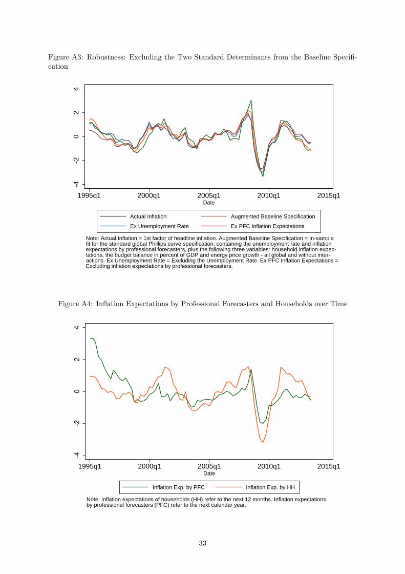
Figure A3: Robustness: Excluding the Two Standard Determinants from the Baseline Specifi-cation
-4-2
02
4
1995q1 2000q1 2005q1 2010q1 2015q1Date
Actual Inflation Augmented Baseline Specification
Ex Unemployment Rate Ex PFC Inflation Expectations
Note: Actual Inflation = 1st factor of headline inflation. Augmented Baseline Specification = In-samplefit for the standard global Phillips curve specification, containing the unemployment rate and inflationexpectations by professional forecasters, plus the following three variables: household inflation expec-tations, the budget balance in percent of GDP and energy price growth - all global and without inter-actions. Ex Unemployment Rate = Excluding the Unemployment Rate. Ex PFC Inflation Expectations =Excluding inflation expectations by professional forecasters.
Figure A4: Inflation Expectations by Professional Forecasters and Households over Time
-4-2
02
4
1995q1 2000q1 2005q1 2010q1 2015q1Date
Inflation Exp. by PFC Inflation Exp. by HH
Note: Inflation expectations of households (HH) refer to the next 12 months. Inflation expectationsby professional forecasters (PFC) refer to the next calendar year.
33

Figure A5: The In-Sample Fit Excluding Household Inflation Expectations but Adding Com-modity Prices
-4-2
02
4
1995q1 2000q1 2005q1 2010q1 2015q1Date
Actual Inflation Augmented Baseline Specification
Repl. HH Infl. Exp. with FPG
Note: HH Infl. Exp. = Household Inflation Expectations. FPG = Food Price Growth. Actual Inflation =1st factor of headline inflation. Augmented Baseline Specification = In-sample fit for the standardglobal Phillips curve specification, containing the unemployment rate and inflation expectations byprofessional forecasters, plus the following three variables: household inflation expectations, thebudget balance in % of GDP (Budget) and energy price growth - all global and without interactions.
Figure A6: Inflation Expectations and the Budget Balance
-4-2
02
4
1995q1 2000q1 2005q1 2010q1 2015q1Date
Inflation Exp. by HH Inflation Exp. by PFC
Budget Bal. in % of GDP
Note: HH = Households. PFC = Professional Forecasters.
34

Figure A7: Robustness: Main In-Sample Predictions Based on the First Factor (Memorandum)
-4-2
02
4
1995q1 2000q1 2005q1 2010q1 2015q1Date
Actual Inflation Baseline Specification
Baseline Specification with HH Exp. Augmented Baseline Specification
Note: Global aggregation is based on 1st factor. Actual Inflation = Global headline inflation. Aug-mented Baseline Specification = In-sample fit for the standard global Phillips curve specification,containing the unemployment rate and inflation expectations by professional forecasters, plusthe following three variables: household inflation expectations, the budget balance in percent ofGDP and energy price growth - all global and without interactions.
Figure A8: Robustness: Main In-Sample Predictions Based on an Unweighted Average
-4-2
02
4
1995q1 2000q1 2005q1 2010q1 2015q1Date
Headline Inflation, unw. Avg. Baseline Specification
Baseline Specification with HH Exp. Augmented Baseline Specification
Note: Global aggregation is based on an unweighted average. Actual Inflation = Global headlineinflation. Augmented Baseline Specification = In-sample fit for the standard global Phillips curvespecification, containing the unemployment rate and inflation expectations by professional fore-casters, plus the following three variables: household inflation expectations, the budget balancein percent of GDP and energy price growth - all global and without interactions.
35

Figure A9: Robustness: Main In-Sample Predictions Based on a Weighted Average
-4-2
02
4
1995q1 2000q1 2005q1 2010q1 2015q1Date
Headline Inflation, w. Avg. Baseline Specification
Baseline Specification with HH Exp. Augmented Baseline Specification
Note: Global aggregation is based on an weighted average. Actual Inflation = Global headline in-flation. Augmented Baseline Specification = In-sample fit for the standard global Phillips curvespecification, containing the unemployment rate and inflation expectations by professional fore-casters, plus the following three variables: household inflation expectations, the budget balancein percent of GDP and energy price growth - all global and without interactions.
Figure A10: Robustness: In-Sample Fit of Key Specifications in a Constant Country Sample
-4-2
02
4
1995q1 2000q1 2005q1 2010q1 2015q1Date
Actual Inflation Baseline Specification
Baseline with HH Infl. Exp. Augmented Baseline Specification
Note: Actual Inflation = 1st factor of headline inflation. Baseline Specification = In-sample fit for thestandard global Phillips curve specification, containing the unemployment rate and inflation expec-tations by professional forecasters. Augmented Baseline Specification = Baseline specification plusthe following three variables: household inflation expectations (HH Exp.), the budget balance in per-cent of GDP (Budget) and energy price growth - all global and without interactions.
36

Figure A11: Robustness: Historical Contributions in a Constant Country Sample
-4-2
02
4
PFC Infl. Exp. HH Infl. Exp.
Unemp. Rate Budget Def.
Energy Pr. Constant
Residual
1995q1 2000q1 2005q1 2010q1 2013q3
Figure A12: Robustness: Country-by-Country Results I
Austria
Belgium
Note: Green Line = Actual Inflation, Red Line = Baseline Specification, Blue Line = Augmented BaselineSpecification. The same color scheme applies to the following two figures.
37

Figure A13: Robustness: Country-by-Country Results II
Denmark France
Germany Italy
Figure A14: Robustness: Country-by-Country Results III
Portugal Spain
United Kingdom United States
38

Figure A15: The Augmented Baseline Specification with Shorter Estimation Samples
-4-2
02
4
1995q1 2000q1 2005q1 2010q1 2015q1Date
Actual Inflation Augmented Baseline, 2003q1
Augmented Baseline, 2006q1 Augmented Baseline, 2009q1
Augmented Baseline, 20012q1
Note: Actual Inflation = 1st factor of headline inflation. Augmented Baseline Specification = In-samplefit for the standard global Phillips curve specification, containing the unemployment rate and inflationexpectations by professional forecasters, plus the following three variables: household inflation expec-tations, the budget balance in percent of GDP and energy price growth - all global and without inter-actions. Dates indicates the end of the estimation sample. Starting date is 1995q1 in all cases.
39

Figure A16: Repeating the First Selection Procedure at Different Points in Time - Rank
1
6
11
16
21
26
Europ. HH Infl. Exp.
Budget Balance
Energy Price Growth
Note: This figure shows the time-varying rank (out of all 26 tested variables) for the following variables:European Household Inflation Expectations, Budget Balance in % of GDP, and Energy-Price Growth,obtained from running the MSE-minimizing selection procedure at different points in time. Starting pointof the selection procedure is 1995q1 in all cases. The baseline specification to which the third variableis added contains inflation expectations by professional forecasters for the next calendar year and theunemployment rate; i.e., no interaction terms.
Figure A17: Repeating the First Selection Procedure at Different Points in Time - Relative MSE
0.00
0.02
0.04
0.06
0.08
0.10
0.12
0.14
0.16
Europ. HH Infl. Exp.
Budget Balance
Energy Price Growth
Note: This figure shows the time-varying relative MSE (= MSE – MSE of the variable with the lowestMSE) for the variables European Household Inflation Expectations, Budget Balance in % of GDP, andEnergy-Price Growth obtained from running the MSE-minimizing selection procedure at different pointsin time. Starting point of the selection procedure is 1995q1 in all cases. The baseline specification towhich the third variable is added contains inflation expectations by professional forecasters for the nextcalendar year and the unemployment rate in levels; i.e., no interaction terms.
40

Table A1: Literature on Global Inflation Dynamics and Their Determinants
Paper Methodology Data Determinants Result Ciccarelli and Mojon (2005)1
Extraction of the first common factor for headline inflation Bayesian model selection procedure and VAR
22 OECD countries, 1960-2003; two subsamples: 1960-1981 and 1981-2003
Bayesian model: common factors of industrial production,* nominal wages,* short-term interest rates, long-term interest rates, the yield curve, several nominal and real money variables;* VAR: Oil price and all variables marked with a star (*)
Bayesian model: real activity variables are important in the short run and monetary variables in the long run. The most significant variables enter the VAR. VAR: evaluated by a variance decomposition – the results for the overall sample indicate that the oil price, wages and M3 are important; the results for the second subsample show only very little significance.
Hakkio (2009) Extraction of the first two common factors for headline and core inflation Examines whether there is a commonality among determinants
Up to 19 OECD countries, 1961-2008
Cyclical unemployment, cyclical real GDP, real GDP growth, narrow money growth, broad money growth, short-term interest rate, intermediate interest rate, long-term interest rate
Interest rates show the highest degree of commonality, followed by real GDP growth and broad money growth.
Monacelli and Sala (2009)
International common factors for 948 CPI items
In the U.S., Germany, France and the U.K., 1991-2004
Sectoral trade openness The authors find a strongly positive relationship between trade openness at the sectoral level and the exposure of CPI inflation to international shocks.
Mumtaz and Surico (2012)2
Extraction of the first common factor for 164 quarterly price series Dynamic factor model with time-varying parameters and stochastic volatility
13 advanced countries, 1961-2004
Idiosyncratic components and the international component/first factor of inflation
The level and the persistence of inflation are captured by the first common factor, while volatility is driven by country-specific con-ditions.
1 Summary is based on the working paper version. The paper has been published with a slightly different focus in 2010. 2 Summary is based on 2007 WP version.
41

Table A2: Global Variables
Variable # of Countries AUS AUT BEL CAN DEN FIN FRA GER GRE ICE IRE ISR ITA JAP KOR LUX NET NZL NOR POR SPA SWE SWI UK US
InflationHeadline Inflation 25 x x x x x x x x x x x x x x x x x x x x x x x x xCore Inflation 25 x x x x x x x x x x x x x x x x x x x x x x x x x
Inflation ExpectationsHeadline Inflation, backward-looking 25 x x x x x x x x x x x x x x x x x x x x x x x x xCore Inflation, backward-looking 25 x x x x x x x x x x x x x x x x x x x x x x x x xUS Households, 1 year-ahead 25 xUS Households, 5+ years-ahead 25 xOECD Households, 1 year-ahead 11 x x x x x x x x x x xProfessional Forecasters, next year 22 x x x x x x x x x x x x x x x x x x x x x xProfessional Forecasters, 5 years from now 8 x x x x x x x xProfessional Forecasters, 10 years from now 8 x x x x x x x xMarket-based, over the next 5 years 1 xMarket-based, over the next 10+ years 3 x x x
Measures of Economic SlackUnemployment Rate 21 x x x x x x x x x x x x x x x x x x x x xOutput Gap 22 x x x x x x x x x x x x x x x x x x x x x xUnemployment Gap 21 x x x x x x x x x x x x x x x x x x x x xReal GDP Gap 22 x x x x x x x x x x x x x x x x x x x x x xIndustry Production Gap 24 x x x x x x x x x x x x x x x x x x x x x x x xIndustry Production Growth 24 x x x x x x x x x x x x x x x x x x x x x x x xUnit Labor Cost Growth 12 x x x x x x x x x x x xLabor Compensation Growth 14 x x x x x x x x x x x x x x
Other VariablesGov. Budget Balance 21 x x x x x x x x x x x x x x x x x x x x xGrowth of QE-Quantities 1 xInflation Expectations Uncertainty 14 x x x x x x x x x x x x x xFinancial Market Uncertainty 1 xCredit Growth 20 x x x x x x x x x x x x x x x x x x x xReal Estate Price Growth 11 x x x x x x x x x x x
Note: Stock Market, Oil, Energy, and Food Prices are all based on global indices. "x" indicates that data are available.
42

Table A3: Summary Statistics for all Potential Explanatory Variables
Variable Obs Mean Std. Min MaxProfessional Forecasters, next year 75 0 1.0 -2.0 3.3Unemployment Rate 75 0 1.0 -1.6 1.7US Households, 1 year-ahead 75 0 1.0 -3.0 3.9US Households, 5+ years-ahead 75 0 1.0 -1.6 2.7OECD Households, 1 year-ahead 75 0 1.0 -3.2 1.6Professional Forecasters, 5 years from now 75 0 1.0 -1.1 3.7Professional Forecasters, 10 years from now 75 0 1.0 -1.2 3.5Market-based, over the next 5 years 75 0 1.0 -3.6 2.9Market-based, over the next 10+ years 75 0 1.0 -1.7 3.3Output Gaps 75 0 1.0 -1.7 2.2Industry Production Growth 75 0 1.0 -4.0 1.6Unit Labor Cost Growth 75 0 1.0 -2.1 3.9Labor Compensation Growth 75 0 1.0 -2.7 1.8Gov. Budget Balance 75 0 1.0 -2.1 1.4Inflation Expectations Uncertainty 75 0 1.0 -1.6 2.8Headline Inflation, backward-looking 71 0 1.0 -2.8 2.5Core Inflation, backward-looking 71 0 1.0 -1.6 3.1Real GDP Gap 75 0 0.1 -0.3 0.3Unemployment Gap 75 0 0.4 -0.8 0.9Industry Production Gap 75 0 0.3 -1.0 0.6Food Price Growth 75 0.0 0.1 -0.2 0.5Energy Price Growth 75 0.1 0.3 -0.5 1.1Oil Price Growth 75 0.2 0.3 -0.5 1.3Stock Market Price Growth 75 0.1 0.2 -0.4 0.4Growth of QE-Quantities 74 0.3 1.1 -0.1 7.0Real Estate Price Growth 71 -0.1 1.4 -8.8 5.2Credit Growth 71 0.1 1.1 -3.6 6.0Financial Market Uncertainty 75 21.2 7.9 11.0 58.6
Note: National variables are generally standardized (Mean = 0, Std. = 1) owing to the computation of the first factor and are present for 75 observations (1995q1-2013q3). However, when a global variable does not enter in levels (e.g., as gap measure or as growth rate) or a variable is global by definition (e.g., prices), mean, standard deviation and observations can differ slightly.
43

Table A4: Selected Specifications to Support the Overall Robustness
Dependent Variable:Headline InflationUnemployment Rate -0.63*** -0.53*** -0.30** -0.59***
(0.00) (0.00) (0.03) (0.00)Inflation Expectations by PFC, next year 0.56*** 0.58*** 0.21***
(0.00) (0.00) (0.00)Inflation Expectations by US HH, 12 months 0.52*** 0.39***
(0.00) (0.00)Unemp. Rate x Infl. Exp. by US HH 0.24***
(0.00)Infl. Exp. by PFC x Infl. Exp. by US HH 0.04
(0.69)Inflation Expectations by HH, 12 months 0.58*** 0.72***
(0.00) (0.00)Budget Bal. in % of GDP 0.09* -0.21* -0.27**
(0.07) (0.07) (0.01)GR of World Energy Prices 1.07*** 0.86***
(0.00) (0.00)GR of World Energy Prices, 1st lag 0.85***
(0.00)GR of World Food Prices, 1st lag 2.15***
(0.00)Observations 75 75 75 75 75R-squared 0.70 0.66 0.76 0.75 0.79
Note: P-Values in Parentheses. Constant not reported.
(1) (2) (3) (4) (5)
44

Table A5: Varying Global Aggregation Techniques: All Key Specifications
Dependent Variable:
First Factor (1) (2) (3)Unemployment Rate -0.54*** -0.33*** -0.75***
(0.00) (0.00) (0.00)Inflation Expectations by HH, 12 months 0.58*** 0.49***
(0.00) (0.00)Inflation Expectations by PFC, next year 0.71*** 0.34*** 0.47***
(0.00) (0.00) (0.00)Budget Bal. in % of GDP -0.50***
(0.00)GR of World Energy Prices 0.70***
(0.00)Observations 75 75 75R-squared 0.52 0.74 0.86
Unweighted Avg. (1) (2) (3)Unemployment Rate -0.36*** -0.21*** -0.71***
(0.00) (0.01) (0.00)Inflation Expectations by HH, 12 months 0.52*** 0.48***
(0.00) (0.00)Inflation Expectations by PFC, next year 0.67*** 0.42*** 0.50***
(0.00) (0.00) (0.00)Budget Bal. in % of GDP -0.57***
(0.00)GR of World Energy Prices 0.26
(0.27)Observations 75 75 75R-squared 0.51 0.71 0.79
Weighted Avg. (1) (2) (3)Unemployment Rate -0.49*** -0.33*** -0.81***
(0.00) (0.00) (0.00)Inflation Expectations by HH, 12 months 0.38*** 0.35***
(0.00) (0.00)Inflation Expectations by PFC, next year 0.58*** 0.36*** 0.34***
(0.00) (0.00) (0.00)Budget Bal. in % of GDP -0.60***
(0.01)GR of World Energy Prices 1.06***
(0.00)Observations 75 75 75R-squared 0.50 0.59 0.79
Headline Inflation
Note: P-Values in Parentheses. Constant not reported.
45

Table A6: Constant Country Sample: Baseline Specification and Post-Crisis Dummy
Dependent Variable:Headline InflationUnemployment Rate -0.32*** -0.40*** -0.96*** -0.97*** -0.91***
(0.00) (0.00) (0.00) (0.00) (0.00)Inflation Expectations by PFC, next year 0.67*** 1.00 0.99*** 1.00 0.91***
(0.00) (.) (0.00) (.) (0.00)Post-Crisis Dummy 1.75*** 1.76*** 2.47***
(0.00) (0.00) (0.00)Unemployment Rate x Post-Crisis Dummy 0.26 0.26 -0.13
(0.41) (0.40) (0.50)Infl. Exp. By PFC x Post-Crisis Dummy 0.98***
(0.00)Observations 75 75 75 75 75R-squared 0.44 0.76 0.81
(1) (2) (3) (4) (5)
Note: P-Values in Parentheses. Constant not reported.
Table A7: Constant Country Sample: Construction of the Augmented Baseline Specification
Dependent Variable:Headline InflationUnemployment Rate -0.25*** -0.19** -0.57*** -0.46***
(0.00) (0.01) (0.00) (0.00)Inflation Expectations by PFC, next year 0.36*** 0.37*** 0.29*** 0.30***
(0.00) (0.00) (0.00) (0.00)Inflation Expectations by HH, 12 months 0.62*** 0.60*** 0.72*** 0.65***
(0.00) (0.00) (0.00) (0.00)Unemp. Rate x Infl. Exp. by HH 0.12
(0.18)Infl. Exp. By PFC x Infl. Exp. by HH 0.04
(0.49)Budget Bal. in % of GDP -0.50*** -0.42***
(0.00) (0.00)GR of World Energy Prices 0.66***
(0.00)Observations 75 75 75 75R-squared 0.73 0.72 0.79 0.82
(2) (3) (4)
Note: P-Values in Parentheses. Constant not reported.
(1)
46

7 References
Aizenman, J. and N. Marion, 2011. “Using inflation to erode the US public debt,” Journal of
Macroeconomics, 33(4), pp. 524-541.
Ball, L. and S. Mazumder, 2011. “Inflation Dynamics and the Great Recession,” Brookings
Papers on Economic Activity, 42(1), pp. 337-405.
Borio, C., P. Disyatat, and M. Juselius, 2013. “Rethinking potential output: Embedding infor-
mation about the finanical cycle,” BIS Working Papers, No. 404.
Christiano, L. J., M. Eichenbaum, and M. Trabandt, 2014. “Understanding the Great Reces-
sion,” NBER Working Papers, No. 20040.
Ciccarelli, M. and B. Mojon, 2005. “Global Inflation,” ECB Working Paper #0537. The pa-
per has been published with a slightly different focus in 2010 in The Review of Economics and
Statistics, 92(3), pp. 524-535.
Coibion, O. and Y. Gorodnichenko, 2013. “Is The Phillips Curve Alive and Well After All?
Inflation Expectations and the Missing Disinflation,” mimeo. Forthcoming in Gertler, 2014.
“Lessons from the Financial Crisis for Monetary Policy.”
Dahlhaus, T., K. Hess, and A. Reza, 2014. “International Transmission Channels of US Quan-
tiative Easing: Evidence from Canada,” mimeo.
Del Negro, M., M. P. Giannoni, and F. Schorfheide, 2014. “Inflation in the Great Recession and
New Keynesian Models,” NY FED Staff Report, No. 618.
Ehrmann, M., D. Pfajfar and E. Santoro, 2014. “Consumer Attitudes and the Epidemiology of
Inflation Expectations,” Bank of Canada Working Paper, No. 28.
Eickmeier, S. and K. Pijenburg, 2013. “The Global Dimension of Inflation – Evidence from
Factor-Agumented Phillips Curves,” Oxford Bulletin of Economics and Statistics, 75(1), pp.
103-122.
Ferroni, F. and B. Mojon 2014. “Domestic and Global Inflation,” mimeo.
Gilchrist, S., R. Schoenle, J. W. Sim, and E. Zakrajssek, 2014. “Inflation Dynamics During the
Financial Crisis,” mimeo.
Gordon, R., 2013. “The Phillips Curve is Alive and Well: Inflation and the NAIRU During the
Slow Recovery,” NBER Working Paper, No. 19390.
Hakkio, C., 2009. “Global Inflation Dynamics,” Federal Reserve Bank of Kansas City Working
Paper.
Hall, R., 2011. “The Long Slump,” American Economic Review, 101(2), pp. 431-69.
47

King, R. G. and M. W. Watson, 2012. “Inflation and Unit Labor Cost,” Journal of Money,
Credit and Banking, 44, pp. 111-149.
Lagarde, C., 2014. “The Global Economy in 2014,” Speech at the National Press Club, Wash-
ington D.C., January 15, 2014.
Leheyda, N. and F. Verboven, 2013. “Scrapping Subsidies during the Financial Crisis - Evidence
from the Europe”, KU Leuven Discussion Paper Series, No. 13.
Medel, C., M. Pedersen, and Pincheira, 2014. “The Elusive Predictive Ability of Global Infla-
tion,” Bank of Chile Working Paper, No. 725.
Monacelli, T. and L. Sala, 2009. “The International Dimension of Inflation: Evidence from Dis-
aggregated Consumer Price Data,” Journal of Money, Credit and Banking, 41(s1), pp. 101-120.
Mumtaz, H. and P. Surico, 2012. “Evolving International Inflation Dynamics: World And
Country-Specific Factors,” Journal of the European Economic Association, 10(4), pp. 716-734.
Murphy, R., 2014. “Explaining inflation in the aftermath of the Great Recession,” Journal of
Macroeconomics, 40, pp. 228-244.
Svensson, L., 2013. “The Possible Unemployment Cost of Average INflation Below A Credible
Target,” mimeo.
WEO, 2013. “The dog that didnt bark: Has inflation been muzzled or was it just sleeping?,”
World Economic Outlook, Chatper 3.
Williams, J., 2010. “Sailing into Headwinds: The Uncertain Outlook for the U.S. Economy,”
Presentation to a Joint Meeting of the San Francisco and Salt Lake City Branch Boards of
Directors, Salt Lake City, Utah.
48