Glm Sample
31
-
Upload
lulikbrera -
Category
Documents
-
view
251 -
download
3
description
glm sample
Transcript of Glm Sample

Generalized Linear Modeling with H2Orsquos RPackage
H2Oai
This book is for sale at httpleanpubcomglm
This version was published on 2015-02-21
This is a Leanpub book Leanpub empowers authors and publishers with the Lean Publishingprocess Lean Publishing is the act of publishing an in-progress ebook using lightweight tools andmany iterations to get reader feedback pivot until you have the right book and build traction onceyou do
copy2015 H2Oai
Author Biographies
Jessica Lanford Jessica is a word hacker and seasoned technical communicator at H2Oai Shebrings our product to life by documenting the many features and functionality of H2O Havingworked for some of the top companies in technology including Dell ATampT and Lam Research she isan expert at translating complex ideas to digestible articles
Tomas Nykodym Tomas is currently in the process of finishing his PhD at Binghamton UniversityHis area of research is behavioral malware detection He received his undergraduate degree from theCzech Technical University Tomas has worked at IBM-research and Agent-Technology Group Hehas participated on several projects related to malware detectionprotection funded by US Air ForceSpecifically he developed a system for modeling software behavior using compressed graphs of thesystem calls made on the system Tomas also created a sandbox with simulated user activity for safeexecution of malware with advanced behavior extraction algorithms to extract behavior of mal- wareinjected into other processes Apart from his work Tomas spends his time mountain biking skiingsnowboarding and staying active
Ariel Rao Ariel is a data and math hacker intern at H2O She is currently an undergraduate studentat Carnegie Mellon University pursing degrees in Logic amp Computation and Computer Science Herinterests include optimizing automated computation and formal verification
Amy Wang Amy is a math hacker at H2O She graduated from Hunter College in NYC with aMasters in Applied Mathematics and Statistics with a heavy concentration on numerical analysisand financial mathematics Her interest in applicable math eventually lead her to big data andfinding the appropriate mediums for data analysis
Contents
What is H2o 1
What is GLM 2GLM on H2O 2Summary of Features 3
Installation 4Support 6
Generalized Linear Modeling 7Model Fitting 7Model Validation 7Regularization 8Lasso 8Elastic Net Penalty 8
GLM Models 10Linear Regression (Gaussian Family) 10Logistic Regression (Binomial Family) 10Poisson Models 12Gamma Models 13
GLM on H2o 14Input Parameters 14Coefficient Constraints 15H2O GLM Model Output 15Coefficients and Normalized Coefficients 16Validation 17Generating Predictions 17Categorical Variables 17Largest Categorical Trick 18Cross Validation 18Selecting Regularization Parameters 18Grid Search over Alpha 19Lambda Search 19
CONTENTS
Grid Search over Lambdas 19Strong Rules 20Performance Characteristics 20
Use Case Classification with Airline Data 21Airline Dataset Overview 21Loading Data 21Performing a Trial Run 21Extracting and Handling the Results 22Web Interface 23Variable Importances 23Java Model 23
Appendix Parameters 24
References 26
What is H2oH2O is fast scalable open source machine learning and deep learning for Smarter Applications WithH2O enterprises like PayPal Nielsen Cisco and others can use all of their data without samplingand get accurate predictions faster Advanced algorithms like Deep Learning Boosting and BaggingEnsembles are readily available for application designers to build smarter applications throughelegant APIs Some of our earliest customers have built powerful domain-specific predictive enginesfor Recommendations Customer Churn Propensity to Buy Dynamic Pricing and Fraud Detectionfor the Insurance Healthcare Telecommunications AdTech Retail and Payment Systems
Using in-memory compression techniques H2O can handle billions of data rows in-memory ndash evenwith a fairly small cluster The platform includes interfaces for R Python Scala Java JSON andCoffeescriptJavaScript along with its built-in Flow web interface that make it easier for non-engineers to stitch together complete analytic workflows The platform was built alongside (andon top of) both Hadoop and Spark Clusters and is typically deployed within minutes
H2O implements almost all common machine learning algorithms ndash such as generalized linearmodeling (linear regression logistic regression etc) Naive Bayes principal components analysistime series k-means clustering and others H2O also implements best-in-class algorithms such asRandom Forest Gradient Boosting and Deep Learning at scale Customers can build thousands ofmodels and compare them to get the best prediction results
H2O is nurturing a grassroots movement of physicists mathematicians computer and data scientiststo herald the new wave of discovery with data science Academic researchers and Industrial datascientists collaborate closely with our team to make this possible Stanford university giants StephenBoyd Trevor Hastie Rob Tibshirani advise the H2O team to build scalable machine learningalgorithms With 100s of meetups over the past two years H2O has become a word-of-mouthphenomenon growing amongst the data community by a 100- fold and is now used by 12000+users deployed in 2000+ corporations using R Python Hadoop and Spark
Try it out
H2O offers an R package that can be installed from CRAN H2O can be downloaded from httpwwwh2oaidownload
Join the community
Connect with h2ostreamgooglegroupscom and httpsgithubcomh2oai to learn about ourmeetups training sessions hackathons andproduct updates
Learn more about H2O
Visit httpwwwh2oai
What is GLMGeneralized linear models (GLM) are the workhorse for most predictive analysis use cases GLM canbe used for both regression and classification it scales well to large datasets and is based on solidstatistical background It is a generalization of linear models allowing for modeling of data withexponential distributions and for categorical data (classification) GLM models are fitted by solvingthe maximum likelihood optimization problem
GLM on H2O
H2Orsquos GLM algorithm fits the generalized linear model with elastic net penalties The model fittingcomputation is distributed extremely fast and scales extremely well for models with a limitednumber (sim low thousands) of predictors with non-zero coefficients The algorithm can computemodels for a single value of a penalty argument or the full regularization path similar to the glmnetpackage for R Friedman et al H2Orsquos GLM fits the model by solving following problem
minβ
1
Nlog minus likelihood(family β) + λ(α∥β∥1 +
1minus α
2∥β∥22)
The elastic net parameter α controls the penalty distribution between L1 and L2 penalty It can haveany value between 0 and 1 When α = 0 we have no L1 penalty and the problem becomes ridgeregression If α = 1 there is no L2 penalty and we have lasso
The main advantage of an L1 penalty is that with sufficiently high λ it produces a sparse solutionthe L2-only penalty does not reduce coefficients to exactly 0 The two penalties also differ in thecase of correlated predictors The L2 penalty shrinks coefficients for correlated columns towardseach other while the L1 penalty will pick one and drive the others to zero Using the elastic netargument α you can combine these two behaviors It is also useful to always add a small L2 penaltyto increase numerical stability
Similarly to Friedman et al H2O can compute the full regularization path starting from null-model(maximum penalty) going down to minimally penalized model This search is made efficient byemploying strong-rules to filter out inactive coefficients (coefficients pushed to zero by penalty)Computing full regularization path is useful in that it gives more insight about the importance ofindividual coefficients and quality of the model while allowing selection of the optimal amount ofpenalization for the given problem and data
What is GLM 3
Summary of Features
In summary H2Orsquos GLM functionalities include
bull fits generalized linear model with elastic net penaltybull supported GLM families include Gaussian Binomial Poisson and Gammabull efficient handling of categorical variablesbull efficient computation full regularization pathbull efficient distributed n-fold cross validationbull distributed grid search over elastic-net parameter αbull upper and lower bounds for coefficientsbull proximal operator interface
InstallationLoad the latest CRAN H2O package by running
installpackages(h2o)
Alternatively you can (and should for this tutorial) download the latest H2O build by following theldquoInstall in Rrdquo instructions in the H2O download table https3amazonawscomh2o-releaseh2omasterlatesthtml
Open your R Console and run the following to install the latest H2O build in R
1 The following two commands remove any previously installed H2O packages for R
2 gt if (packageh2o in search()) detach(packageh2o unload=TRUE)
3 gt if (h2o in rownames(installedpackages())) removepackages(h2o)
4
5 Next download install and initialize the H2O package for R
6 replace the s below with the release number found on our download page
7 gt installpackages(h2o repos=(c(https3amazonawscomh2o-releaseh2o
8 masterR getOption(repos))))
9
10 Load h2o library in R
11 gt library(h2o)
To launch on a single node initialize H2O on all the cores of your machine with
localH2O = h2oinit(nthreads = -1)
The function h2oinit() will initialize a H2O instance and instantiates a H2O client module Bydefault the H2O instance will launch on localhost54321 To establish a connection to an existingH2O cluster node explicitly state the IP address ip = localhost and port number (port = 54321)in the h2oinit() call
Run the following command to observe an example classification model built through H2Orsquos GLM
Installation 5
1 Build a GLM model on prostate data with formula CAPSULE ~ AGE + RACE + PSA +
2 DCAPS
3 gt prostatePath = systemfile(extdata prostatecsv package = h2o)
4 gt prostatehex = h2oimportFile(localH2O path = prostatePath key = prostateh
5 ex)
6 gt h2oglm(y = CAPSULE x = c(AGERACEPSADCAPS) data = prostatehex
7 family = binomial nfolds = 0 alpha = 05 lambda_search = FALSE use_all_f
8 actor_levels = FALSE variable_importances = FALSE higher_accuracy = FALSE)
The output of the model build will include coefficients as well as some validation statistics
1 IP Address 127001
2 Port 54321
3 Parsed Data Key prostatehex
4
5 GLM2 Model Key GLMModel__827586bb2c59ba79dc129b8500174940
6
7 Coefficients
8 AGE RACE DCAPS PSA Intercept
9 -001104 -063136 131888 004713 -110896
10
11 Normalized Coefficients
12 AGE RACE DCAPS PSA Intercept
13 -007208 -019495 040972 094253 -033707
14
15 Degrees of Freedom 379 Total (ie Null) 375 Residual
16 Null Deviance 5123
17 Residual Deviance 4495 AIC 4595
18 Deviance Explained 012254
19 Best Threshold 028
20
21 Confusion Matrix
22 Predicted
23 Actual false true Error
24 false 75 152 0670
25 true 18 135 0118
26 Totals 93 287 0447
27
28 AUC = 07157151 (on train)
Installation 6
Support
Users of the H2O package may submit general enquiries and bug reports privately to H2O via emailsupporth2oai or publicly post them to h2ostreamgooglegroupscom Specific bugs or issueswill be filed to H2Orsquos JIRA https0xdataatlassiannetsecureDashboardjspa
Generalized Linear ModelingThis section contains a brief overview of generalized linear models and follows up with a few detailsfor each model family
Generalized linear models are generalization of linear regressions Linear regression models thedependency of response y on a vector of predictors x (y sim xTβ + β0) The models are built withthe assumptions that y has a gaussian distribution with a variance of σ2 and the mean is a linearfunction of x with an offset of some constant β0 ie y = N (xTβ + β0 σ
2) These assumptions canbe overly restrictive for real-world data that do not necessarily follow have a gaussian distributionGLM generalizes linear regression in the following ways
bull adds a non-linear link function that transforms the expectation of response variable so thatlink(y) sim xTβ + β0
bull allows variance to depend on the predicted value by specifying the conditional distribution ofthe response variable or the family argument
This generalization allows us to use GLM on problems such as binary classification (Logisticregression)
Model Fitting
GLM models are fitted by maximizing the likelihood For the gaussian family maximum likelihoodis simply the minimal mean squared error which has an analytical solution and can be solved withordinary least squares For all other families the maximum likelihood problem has no analyticalsolution so we must use an iterative method such as IRLSM Newton method gradient descent andL-BFGS
Model Validation
Evaluating the quality of the model is a critical part of any data-modeling and scoring process Thereare several standard ways on how to evaluate the quality of the fitted GLMmodel the most commonmethod is to use the resulting deviance Deviance is calculated by comparing the log likelihood ofthe fitted model with log likelihood of the saturated model (or theoretically perfect model)
deviance = 2(ln(Ls)minus ln(Lm))
Generalized Linear Modeling 8
Another metric frequently used for model selection is the Akaike information criterion (AIC) AICis a measure of the relative quality of a statistical model for a given set of data that is obtainedby calculating the information loss when replacing the original data with the model itself Unlikedeviance which would assign a perfect value for the saturated model and measures the absolutequality of the fit with a comparison against the null-hypothesis it takes into account the complexityof the given model AIC is defined as follows
aic = 2(k minus ln(Lm))
where k is the number of model parameters and ln(Lm) is the log likelihood of the fitted model overthe data
Regularization
We introduce penalties to model-fitting to avoid over-fitting reduce variance of the predictionerror and deal with correlated predictors There are two common penalized linear models RidgeRegression and Lasso Ridge regression provides greater numerical stability and is easier (faster) tocompute On the other hand Lasso leads to a sparse solution which is a big advantage in manysituations as it can be used for feature selection and to produce models with fewer parametersWhen encountering highly correlated columns the L2 penalty tends to push all of the coefficientstowards each other while the L1 penalty will pick one and remove the others (0 coefficients)
Lasso
Lasso represents the L1 penalty and is an alternative regularized least squares method that uses theconstraint ||B||1 The penalty is configured using the alpha parameter The main difference betweenlasso and ridge regression is that as the penalty for ridge regression increases the parameters arereduced to non-zero values With lasso if the penalty is increased the parameters can be reducedto zero values Since reducing parameters to zero removes them from the model the lasso methodprovides only the relevant data Ridge regression never removes any data
Elastic Net Penalty
H2O supports elastic net regularization which is parametrized by alpha and lambda arguments(similarly to glmnet)
The alpha argument controls the elastic net penalty distribution to L1 and L2 norms It can haveany value in [01] range (inclusive) or a vector of values (triggers grid search) Alpha = 0 leads toRidge Regression alpha = 1 leads to LASSO
Generalized Linear Modeling 9
The lambda argument controls the penalty strength it can have any positive value or a vector ofvalues (which triggers grid search) Note Lambda values are capped at λmax which is the smallestλ st the solution is empty model (all zeros except for intercept)
Elastic net combines the two and adds another parameter α which controls distribution of thepenalty between L1 and L2 The combination of the two penalties is beneficial since L1 gives sparsitywhile L2 gives stability and encourages the grouping effect (where a group of correlated variablestends to be dropped or added into the model all at once)One possible use of the α argument is todo lasso with very little L2 penalty (α almost 1) to stabilize the computation (improve convergencespeed)
Model-fitting problem with elastic net penalty becomes
minββ0
1
Nln(L(family β β0)) + λ(α∥β∥1 +
1minus α
2∥β∥22)
GLMModelsThe following section describes GLM families supported in H2O
Linear Regression (Gaussian Family)
Linear regression refers to the gaussian family model It is the simplest example of GLM but ithas many uses and several advantages over the other families such as faster and more stablecomputation
It models the dependency as a purely linear function (with link = identity) y = xTβ + β0
The model is fitted by solving the least squares problem (maximum likelihood for gaussian family)
minββ0
1
2N
Nsumi=1
(xTi β + β0 minus yi)
T (xTi β + β0 minus yi) + λ(α∥β∥1 +
1minus α
2)∥β∥22
Deviance is simply the sum of squared errorsD =Nsumi=1
(yi minus yi)2
E
Included in the H2O package is a prostate cancer data set The data was collected for a study doneby Dr Donn Young at The Ohio State University Comprehensive Cancer Center of patients withvarying degrees of prostate cancer Below a model is built to predict the volume (VOL) of tumorsobtained from ultrasounds based on features such as age and race
1 gt filepath = systemfile(extdata prostatecsvpackage = h2o)
2 gt prostatehex = h2oimportFile(object = localH2O filepath key = prostatehex
3 )
4 gt gaussianfit = h2oglm(x = c(AGE RACE PSA GLEASON) y = VOL data
5 = prostatehex family = gaussian)
Logistic Regression (Binomial Family)
Logistic regression can be used in case of a binary classification problem where the response iscategorical with two levels It models dependency as Pr(y = 1|x) The canonical link for binomial
GLM Models 11
family is logit (log of the odds) and its inverse is a logistic function that takes any real number onthe input and projects it onto the 01 range (s-curve) The s-curve is shown below
S-curve
y = Pr(y = 1|x) = exT β+β0
1 + exT β+β0
or alternatively
logy
1minus y= log
Pr(y = 1|x)Pr(y = 0|x)
= xTβ + β0
Themodel is fitted by solvingminββ0
1N
Nsumi=1
(yi(xTi β + β0)minus log(1 + ex
Ti β+β0) + λ(α∥β∥1 + 1minusα
2)∥β∥22
GLM Models 12
Deviance is -2 log likelihood D = minus2Nsumi=1
(ylog(y) + (1minus y)log(1minus y))
E
Using the prostate data set build a binomial model that classifies if there is penetration of theprostatic capsule (CAPSULE) Make sure the entries in the CAPSULE column are binary entriesby using the h2otable() function Change the regression by setting the family to binomial
1 gt h2otable(prostatehex[CAPSULE])
2 rownames Count
3 1) 0 227
4 2) 1 153
5 gt binomialfit = h2oglm(x = c(AGE RACE PSA GLEASON) y = CAPSULE
6 data = prostatehex family = binomial)
Poisson Models
Poisson regression is generally used in cases where the response represents counts and we assumeerrors have a Poisson distribution In general it can be applied to any data where the response isnon-negative
When building a Poisson model we usually model dependency of the mean on the log scale iecanonical link is log and prediction is
y = exT β+β0
The model is fitted by solving
minββ0
1
N
Nsumi=1
(yi(xTi β + β0)minus ex
Ti β+β0) + λ(α∥β∥1 +
1minus α
2)∥β∥22
Deviance is
D = minus2Nsumi=1
(ylog(y)minus y minus y
E
Load the Insurance data from the MASS library and import into H2O Run a poisson model thatpredicts the number of claims (Claims) based on the district of the policy holder (District) their age(Age) and the type of car they own (Group)
GLM Models 13
1 gt library(MASS)
2 gt data(Insurance)
3 gt insurancehex = ash2o(localH2O Insurance)
4 gt poissonfit = h2oglm(x = c(District Group Age) y = Claims data =
5 insurancehex family = poisson)
Gamma Models
The gamma distribution is useful for modeling a positive continuous response variable where theconditional variance of the response grows with its mean but the coefficient of variation of theresponse σ2(x)frac14(x) is constant for all x ie it has a constant coefficient of variation
It is usually used with inverse or log link inverse is the canonical link
The model is fitted by solving
minββ0
1
N
Nsumi=1
yi(xT
i β + β0)minus log(xT
i β + β0) + λ(α∥β∥1 +1minus α
2)∥β∥22
Deviance is
D = minus2Nsumi=1
log(yiyi)minus yi minus yi
yi
E To change the link function from the default inverse function to the log link functionmodify the link argument
1 gt gammainverse lt- h2oglm(x=c(AGERACECAPSULEDCAPSPSAVOL) y=D
2 PROS data=prostatehex family=gamma link=inverse)
3
4 gt gammalog lt- h2oglm(x=c(AGERACECAPSULEDCAPSPSAVOL) y=DPROS
5 data=prostatehex family=gamma link=log)
GLM on H2oThis section describes the specifics of GLM implementation on H2O such as selecting regularizationparameters and handling of categoricals
H2Orsquos GLM implementation presents a high-performance distributed algorithm which scaleslinearly with the number of rows and works extremely well for datasets with limited number ofactive predictors
Input Parameters
Predictors and Response
Every model must specify its predictors and response It is the equivalent formula object in RPredictors and response are specified by source and x and y parameters with an optional offsetparameter
source refers to a frame containing a training dataset All predictors and the response (and offsetif there is one) must be part of this frame
x contains the list of column names or column indices referring to vectors from the source frame itcan not contain periods
y is a column name or index referring to a vector from the source frame
offset is a column name or index referring to a vector from the source frame
Family and Link
Family and Link are both optional parameters The default family is Gaussian and the default
link is a canonical link for the selected family These are passed in as strings
eg family=gamma link = log While it is possible to select something other than a canonicallink it can lead to an unstable computation Recommended combinations are Gaussian and Log orInverse and Gamma with log
Lambda Search
Lambda search is special case of automatic and efficient grid search over lambda argument and isdescribed in its own section Lambda search can be enabled by using the lambda_search = T optionIt can be further parametrized by the n_lambdas and lambda_min_ratio parameters n_lambdasspecifies the number of lambda values on the regularization path lambda_min_ratio specifies theminimal lambda value to be computed as a ration of λmax
GLM on H2o 15
Coefficient Constraints
Coefficient constraints allow you to set special conditions over the model coefficients Currentlysupported constraints are upper and lower bounds and proximal operator interface Parikh and Boyd
The constraints are specified as a frame with following vecs (matched by name all vecs can besparse)
bull names (mandatory) - coefficient namesbull lower_bounds (optional) - coefficient lower bounds must be lt= 0bull upper_bounds (optional) - coefficient upper bounds must be gt= 0bull beta_given (optional) - specifies the given solution in proximal operator interfacebull rho (mandatory if beta_given is specified otherwise ignored) - specifies per-column L2penalties on the distance from the given solution
The proximal operator interface allows you to run the GLM with a proximal penalty on a distancefrom a specified given solution It has various uses for example it can be used as part of ADMMconsensus algorithm to obtain unified solution over separate H2O clouds or in Bayesian regressionapproximation
H2O GLMModel Output
The detailed output of the GLM model varies depending on the distribution used for the modelIn general there are common parts of the output for all Families Coefficients amp NormalizedCoefficients Validation and Prediction Wersquoll cover the model output from an R userrsquos point ofview
First letrsquos build a simple GLM on a small dataset and see what we get out
1 library(h2o)
2
3 instantiate h2o
4 h lt- h2oinit()
5
6 path to the data
7 path is split up so its document friendly
8 databucket lt- httpsrawgithubusercontentcomh2oaih2omastersmalldata
9 datapath lt- paste(databucket logregprostate_traincsv sep = )
10
11 import the data from the url
12 hex lt- h2oimportFile(h datapath)
GLM on H2o 16
13
14 build a binomial regression
15 m lt- h2oglm(x = 39 y = 2 data = hex family = binomial) no other featur
16 es tweaked yet
The default show of this model has the following output
1 IP Address 127001
2 Port 54321
3 Parsed Data Key prostate_trainhex
4
5 GLM2 Model Key GLMModel__8b954fd700d924f3e9dee8717b8246ef
6
7 Coefficients
8 AGE RACE DPROS DCAPS PSA VOL GLEASON Intercept
9 -007668 -010320 059479 013549 043841 -022215 119657 -049458
10
11 Normalized Coefficients
12 AGE RACE DPROS DCAPS PSA VOL GLEASON Intercept
13 -007668 -010320 059479 013549 043841 -022215 119657 -049458
14
15 Degrees of Freedom 304 Total (ie Null) 297 Residual
16 Null Deviance 4121
17 Residual Deviance 3019 AIC 3179
18 Deviance Explained 026733
19 Best Threshold 044
20
21 Confusion Matrix
22 Predicted
23 Actual false true Error
24 false 147 34 0188
25 true 32 92 0258
26 Totals 179 126 0216
27
28 AUC = 08318927 (on train)
Briefly the output contains the IP address and port number of the H2O cluster where the model wastrained It includes the data key the model key the coefficients and some model metrics Letrsquos lookat these more in-depth
Coefficients and Normalized Coefficients
Coefficients are the predictor weights ie the actual model used for prediction
GLM on H2o 17
If the standardize option is set H2O returns another set of coefficients Normalized CoefficientsThese are the predictor weights of the standardized data and are included only for informative pur-poses (eg to compare relative variable importance) In this case the Coefficients are obtained fromNormalized Coefficients by reversing the data standardization process (de-scaled intercept adjustedby added offset) so that they can be applied to data in its original form (ie no standardization priorto scoring) Note These are not the same as coefficients of a model built on non-standardized data
Validation
H2Orsquos GLM performs 10-fold cross-validation by default It does this by generating additionalmodels with 110 of the original data This is fast and gives some idea of how the model willgeneralize However itrsquos always best to evaluate the model using some holdout data
Generating Predictions
The following R code generates predictions
1 testpath lt- paste(databucket logregprostate_testcsv sep = )
2
3 import the data from the url
4 test lt- h2oimportFile(h testpath)
5
6 generate the predictions
7 predictions lt- h2opredict(m test)
8
9 look at the first 6 entries of predictions
10 predictions
11
12 generate the model metrics
13 h2operformance(data=predictions[3] reference=test[1])
Categorical Variables
When applying linear models to datasets with categorical variables the usual approach is to expandthe categoricals into a set of binary vectors with one vector per each categorical level (eg by callingmodelmatrix in R) H2O performs similar expansions automatically and no prior changes to thedataset are needed Each categorical column is treated as a set of sparse binary vectors
GLM on H2o 18
Largest Categorical Trick
Categoricals have special handling during GLM computation as well When forming the grammatrix we can exploit the fact that columns belonging to the same categorical never co-occur andthe gram matrix region belonging to these columns will not have any non-zero elements outsideof the diagonal We can thus keep it in sparse representation taking only O(N) elements insteadof O(NN) Furthermore the complexity of Choelsky decomposition of a matrix that starts with adiagonal region can be greatly reduced H2Orsquos GLM exploits these two facts to handle the largestcategorical ldquofor freerdquo Therefore when analyzing the performance of GLM in the equation expressedabove we can subtract the size of the largest categoricals from the number of predictors
N =sumcisinC
(|| cdomain ||)minus argmaxcisinC
|| cdomain || + || Nums ||
Cross Validation
All validation values can be computed either on the training data set (the default) or using nfoldcross-validation (nfolds gt 1) When using nfold cross-validation we randomly split data into nequally-sized parts and train each of the n models on n-1 parts and compute validation on the partwhich was not used for trainingThe reported validation parameters are then obtained as follows
bull null deviance is sum of null deviances of n-models (each uses null model based on the subsetof the data)
bull residual deviance is sum of residual deviances of all n-modelsbull AIC is based on log-likelihood which is summed up similarly to deviancebull AUC is based on ROC curve build by summing up confusion matrices built for all n-models
This means for each threshold we get a confusion matrix that includes all the rows from the trainingset However each row is classified exclusively by the model that did not have it in its training setThe computation of AUC itself is then the same as in a non-cross-validated case
Selecting Regularization Parameters
To get the best possible model we need to find the optimal values of the regularization parametersαand λ To this end H2O provides grid search over α and a special form of grid search called ldquolambdasearch over λrdquo The recommended way to find optimal regularization settings on H2O is to do a gridsearch over a few α values with an automatic lambda search for each α Both are described belowin greater detail
GLM on H2o 19
Grid Search over Alpha
Alpha search is not always needed and simply changing its value to 05 (or 0 or 1 if we only wantRidge or Lasso respectively) works in most cases If α search is needed usually only a few valuesare sufficient Alpha search is invoked by supplying a list of values for α instead of a single valueH2O then produces one model per α value The grid search computation can be done in parallel(depending on the cluster resources) and it is generally more efficient than computing differentmodels separately from R
Use caution when including α = 0 or α = 1 in the grid search α = 0 will produce a densesolution and it can be really slow (or even impossible) to compute in large N situations α = 1 hasno L2 penalty so it is therefore less numerically stable and can be very slow as well due to slowerconvergence In general it is safer to run with alpha = 1minus ϵ instead
Lambda Search
Lambda search can be enabled by using the lambda_search = T option It can be further parametrizedby the n_lambdas and lambda_min_ratio parameters When this option is enabled H2O performs aspecialized grid search over the list of n_lambdas λ values producing one model each per λ value
The λ-list is automatically generated as an exponentially decreasing sequence going from λmax thesmallest λ stthe solution is a model with all 0s to λmin = lambda_min_ratio λmax
H2O computes λ-models sequentially and in decreasing order warm-starting the model for λk withthe solution for λkminus1 By warm-starting the models we get better performance typically models forsubsequent λs are close to each other so we need only a few iterations per λ (typically 2 or 3) Wealso achieve greater numerical stability since models with a higher penalty are easier to computeso we start with an easy problem and then keep making only small changes to it
Note nlambda lambdaminratio also specify the relative distance of any two lambdas in thesequence This is important for the application of recursive strong rules which are only effectiveif the neighbouring lambdas are ldquocloserdquo to each other The default values are nlambda = 100 andλmin = λmax1e
minus4 which gives us the ratio of 0912 In order for strong rules to work you shouldkeep the ratio close to the default
Grid Search over Lambdas
While automatic lambda search is the preferred method it is also possible to do a grid search overlambda values by passing in vector of lambdas and disabling the lambda-search option The behaviorwill be identical to lambda search except H2O will use a user-supplied list of lambdas instead (stillcapped at λmax)
GLM on H2o 20
Strong Rules
H2Orsquos GLM employs strong rules to discard predictors that are likely to have 0 coefficients prior tomodel building According to strong rules we can identify such predictors based on a gradient withgreat accuracy (very few false negatives and virtually no false positives in practice) greatly reducingthe computational complexity of model fitting and enabling it to run on wide datasets with tens ofthousands of predictors provided that there is a limited number of active predictors
When applying the strong rules we evaluate the gradient at the starting solution filter out inactivecoefficients and fit a model using only a subset of the available predictors Since strong rules mayhave false positives (which are extremely rare in practice) we need to check the solution by testingthe kkt conditions and verify that all discarded predictors indeed have 0 coefficients
Performance Characteristics
The implementation is based on iterative reweighted least squares with ADMM inner solver to dealwith L1 penalty Every iteration of the algorithm consists of following steps
1 Generate weighted least squares problem based on previous solution ie vector of weights wand response z
2 Compute the weighted gram matrixXTWX and XT z vector3 Decompose the gram matrix (Cholesky decomposition) and apply ADMM solver to solve the
L1 penalized least squares problem
Steps 1 and 2 are performed distributively and step 3 is computed in parallel on a single node Wecan thus characterize the computational complexity and scalability of dataset with M observationsand N columns (predictors) on a cluster with n nodes with p CPUs each as follows
O(MN2
pn+
N3
p)
And the overall memory cost is given by
O(MN +N2pn)
In case of M gtgt N we can forget the second term and the algorithm scales linearly both in thenumber of nodes and number of CPUs per node However the equation above also implies thatour algorithm is limited in the number of predictors it can handle since the size of the Gram matrixgrows quadratically (due to a memory and network throughput issue) with the number of predictorsand its decomposition cost grows as the cube of the number of predictors (which is computationalcost issue) H2O can get around these limitations in many cases due to its handling of categoricalsand by employing strong rules to filter out inactive predictors both are described later in this chapter
Use Case Classification with AirlineDataAirline Dataset Overview
The Airline dataset can be downloaded herehttpsgithubcomh2oaih2oblobmastersmalldataairlinesallyears2k_headerszip Remember to save the csv file to your working directory by clickingldquoView Rawrdquo Before running the Airline demo wersquoll first review how to load data with H2O
Loading Data
Loading a dataset in R for use with H2O is slightly different from the usual methodologybecause we must convert our datasets into H2OParsedData objects In this example we will usea toy weather dataset that can be downloaded here httpsrawgithubusercontentcomh2oaih2omastersmalldataweathercsv
First load the data to your current working directory in your R Console (do this for any futuredataset downloads) and then run the following command
weatherhex = h2ouploadFile(localH2O path = weathercsv header = TRUE sep =
key = weatherhex)
To see a quick summary of the data run the following command
summary(weatherhex)
Performing a Trial Run
Returning to the Airline dataset demo we first load the dataset into H2O and select the variableswe want to use to predict a chosen response For example we can model if flights are delayed basedon the departurersquos scheduled day of the week and day of the month
Use Case Classification with Airline Data 22
1 library(h2o)
2 localH2O = h2oinit(nthreads = -1)
3 Load the data and prepare for modeling
4 air_trainhex = h2ouploadFile(localH2O path = ~DownloadsAirlinesTraincsv
5 header = TRUE sep = key = airline_trainhex)
6 air_testhex = h2ouploadFile(localH2O path = ~DownloadsAirlinesTestcsv h
7 eader = TRUE sep = key = airline_testhex)
8 x = c(fYear fMonth fDayofMonth fDayOfWeek UniqueCarrier Origin
9 Dest Distance)
10 y = IsDepDelayed
Now we train the GLM model
1 airlineglm lt- h2oglm(x=x
2 y=y
3 data=air_trainhex
4 key = glm_model
5 family=binomial
6 lambda_search = TRUE
7 return_all_lambda = TRUE
8 use_all_factor_levels = TRUE
9 variable_importances = TRUE)
Extracting and Handling the Results
We can extract the parameters of our model examine the scoring process and make predictions onnew data
1 print(Predict on GLM model)
2 best_glm = airlineglmmodels[[airlineglmbest_model]]
3 airresults = h2opredict(object = best_glm newdata = air_testhex)
4 print(Check performance and AUC)
5 perf = h2operformance(airresults$YESair_testhex$IsDepDelayed )
6 print(perf)
7 perfmodel$auc
8 print(Show distribution of predictions with quantile)
9 quant = quantileH2OParsedData(airresults$YES)
10 print(Extract strongest predictions)
11 topair lt- h2oassign(airresults[airresults$YES gt quant[75]] key=topair)
12 topair
Use Case Classification with Airline Data 23
Once we have a satisfactory model the h2opredict() command can be used to compute and storepredictions on the new data which can then be used for further tasks in the interactive modelingprocess
1 Perform classification on the held out data
2 prediction = h2opredict(object = best_glm newdata=air_testhex)
3 Copy predictions from H2O to R
4 pred = asdataframe(prediction)
5 head(pred)
Web Interface
H2O R users have access to an intuitive web interface that mirrors the model building process in RAfter loading data or training a model in R point your browser to your IP address and port number(eg localhost54321) to launch the web interface From here you can clickAgtJ to view yourspecific model details You can also click on Dgt$$textscView All to track datasets currentlyin use
Variable Importances
One useful feature is the variable importances option which can be enabled with the additionalargument importance=TRUE This feature allows us to view the absolute and relative predictivestrength of each feature in the prediction task From R you can access these strengths with thecommand airmodelmodel$varimp You can also view a visualization of the variable importanceson the web interface
Java Model
Java models are currently not available for GLM
To download the model
1 Open the terminal window2 Create a directory where the model will be saved3 Set the new directory as the working directory4 Follow the curl and java compile commands displayed in the instructions at the top of the
Java model
Appendix Parametersbull x A vector containing the names of the predictors in the model No defaultbull y The name of the response variable in the model No defaultbull data An H2OParsedData object containing the training data No defaultbull key The unique hex key assigned to the resulting model If none is given a key willautomatically be generated
bull family A description of the error distribution and corresponding link function to be used inthe model Currently Gaussian binomial Poisson gamma and Tweedie are supported Whena model is specified as Tweedie users must also specify the appropriate Tweedie power Nodefault
bull link The link function relates the linear predictor to the distribution function Default is thecanonical link for the specified family The full list of supported links
ndash gaussian identity log inversendash binomial logit logndash poisson log identityndash gamma inverse log identityndash tweedie tweedie
bull nfolds A logical value indicating whether the algorithm should conduct classificationOtherwise regression is performed on a numeric response variable
bull nfolds Number of folds for cross-validation Default is 0bull validation An H2OParsedData object indicating the validation dataset used to constructconfusion matrix If blank the default is the training data
bull alpha The elastic-net mixing parameter which must be in [01] The penalty is defined to beP (α β) = (1 minus α)2||β||22 + α||β||1 =
sumj[(1 minus α)2β2
j + α|βj|] so alpha=1 is the lassopenalty while alpha=0 is the ridge penalty Default is 05
bull nlambda The number of lambda values when performing a search Default is -1bull lambdaminratio Smallest value for lambda as a fraction of lambdamax the entry valuewhich is the smallest value for which all coefficients in the model are zero Default is -1
bull lambda The shrinkage parameter which multiplies P (α β) in the objective The largerlambda is the more the coefficients are shrunk toward zero (and each other) Default is 1e-5
bull epsilon Number indicating the cutoff for determining if a coefficient is zero Default is 1e-4bull standardize Logical value indicating whether the data should be standardized (set to mean= 0 variance = 1) before running GLM Default is true
bull prior Prior probability of class 1 Only used if family = binomial Default is the frequencyof class 1 in the response column
Appendix Parameters 25
bull variable_importances A logical value (either TRUE or FALSE) to indicate whether thevariable importances should be computed Compute variable importances for input featuresNOTE If use_all_factor_levels is disabled the importance of the base level will NOT beshown Default is false
bull use_all_factor_levels A logical value (either TRUE or FALSE) to indicatewhether all factorlevels should be used By default the first factor level is skipped from the possible set ofpredictors Set this flag if you want use all of the levels Note Needs sufficient regularizationto solve Default is false
bull tweediep The index of the power variance function for the tweedie distribution Only usedif family = tweedie Default is 15
bull itermax Maximum number of iterations allowed Default is 100bull higher_accuracy A logical value indicating whether to use line search This will cause thealgorithm to run slower so generally it should only be set to TRUE if GLM does not convergeotherwise Default is false
bull lambda_search A logical value indicating whether to conduct a search over the space oflambda values starting from lambda_max When this is set to TRUE lambdawill be interpretedas lambda_min Default is false
bull return_all_lambda A logical value indicating whether to return every model built duringthe lambda search Only used if lambda_search = TRUE If return_all_lambda = FALSEthen only the model corresponding to the optimal lambda will be returned Default is false
bull max_predictors When lambda_search = TRUE the algorithmwill stop training if the numberof predictors exceeds this value Ignored when lambda_search = FALSE or max_predictors= -1 Default is -1
bull offset Column to be used as an offset if you have one No defaultbull has_intercept A logical value indicating whether or not to include the intercept term Ifthere are factor columns in your model then the intercept must be included Default is true
ReferencesJerome Friedman Trevor Hastie Rob Tibshirani Regularization Paths for Generalized LinearModels via Coordinate Descent April 29 2009
Robert Tibshirani Jacob Bien Jerome Friedman Trevor Hastie Noah Simon Jonathan Taylor andRyan J Tibshirani Strong Rules for Discarding Predictors in Lasso-type Problems J R StatistSoc B vol 74 2012
Hui Zou and Trevor Hastie Regularization and variable selection via the elastic net J R StatistSoc B (2005) 67 Part 2 pp 301320
Robert Tibshirani Regression Shrinkage and Selection via the Lasso Journal of the RoyalStatistical Society Series B (Methodological) Volume 58 Issue 1 (1996) 267-288
S Boyd N Parikh E Chu B Peleato and J Eckstein Distributed Optimization and StatisticalLearning via the Alternating Direction Method of Multipliers Foundations and Trends inMachine Learning 3(1)1122 2011(Original draft posted November 2010)
N Parikh and S Boyd Proximal Algorithms Foundations and Trends in Optimization 1(3)123-231 2014
httpgithubcomh2oaih2ogit
httpdocsh2oai
httpsgroupsgooglecomforumforumh2ostream
httph2oai
https0xdataatlassiannetsecureDashboardjspa
- Table of Contents
- What is H2o
- What is GLM
-
- GLM on H2O
- Summary of Features
-
- Installation
-
- Support
-
- Generalized Linear Modeling
-
- Model Fitting
- Model Validation
- Regularization
- Lasso
- Elastic Net Penalty
-
- GLM Models
-
- Linear Regression (Gaussian Family)
- Logistic Regression (Binomial Family)
- Poisson Models
- Gamma Models
-
- GLM on H2o
-
- Input Parameters
- Coefficient Constraints
- H2O GLM Model Output
- Coefficients and Normalized Coefficients
- Validation
- Generating Predictions
- Categorical Variables
- Largest Categorical Trick
- Cross Validation
- Selecting Regularization Parameters
- Grid Search over Alpha
- Lambda Search
- Grid Search over Lambdas
- Strong Rules
- Performance Characteristics
-
- Use Case Classification with Airline Data
-
- Airline Dataset Overview
- Loading Data
- Performing a Trial Run
- Extracting and Handling the Results
- Web Interface
- Variable Importances
- Java Model
-
- Appendix Parameters
- References
-
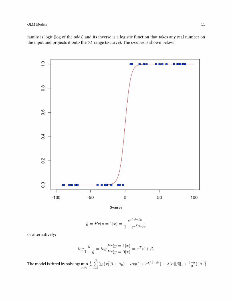
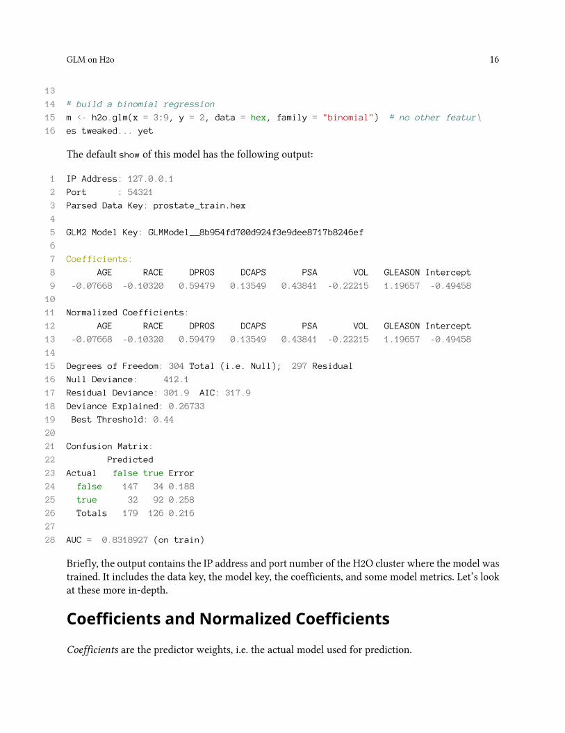
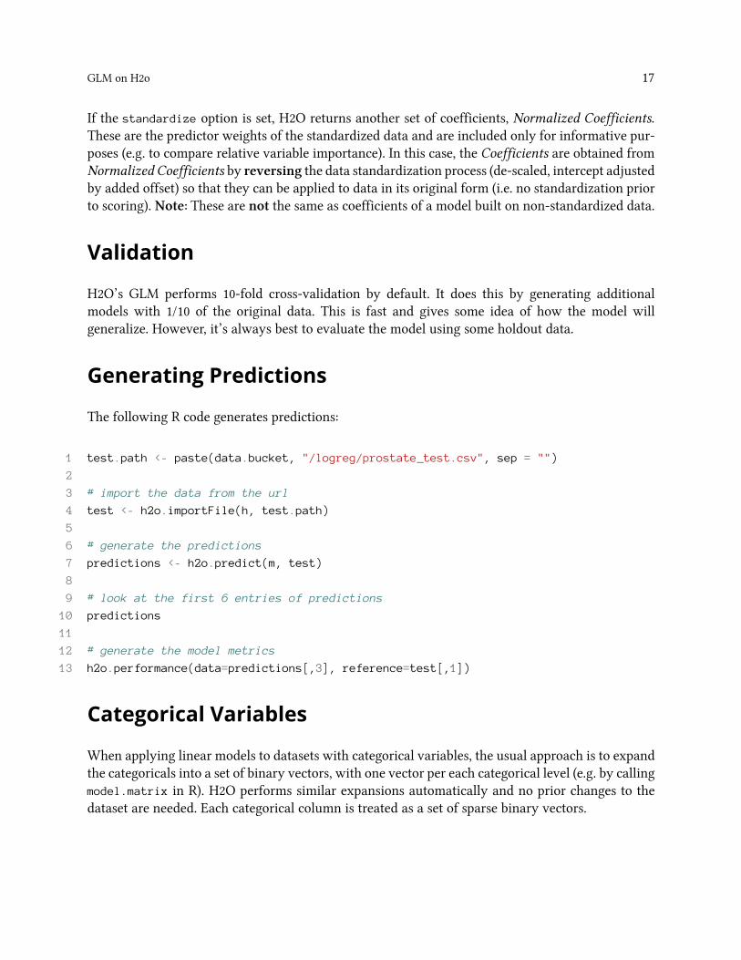
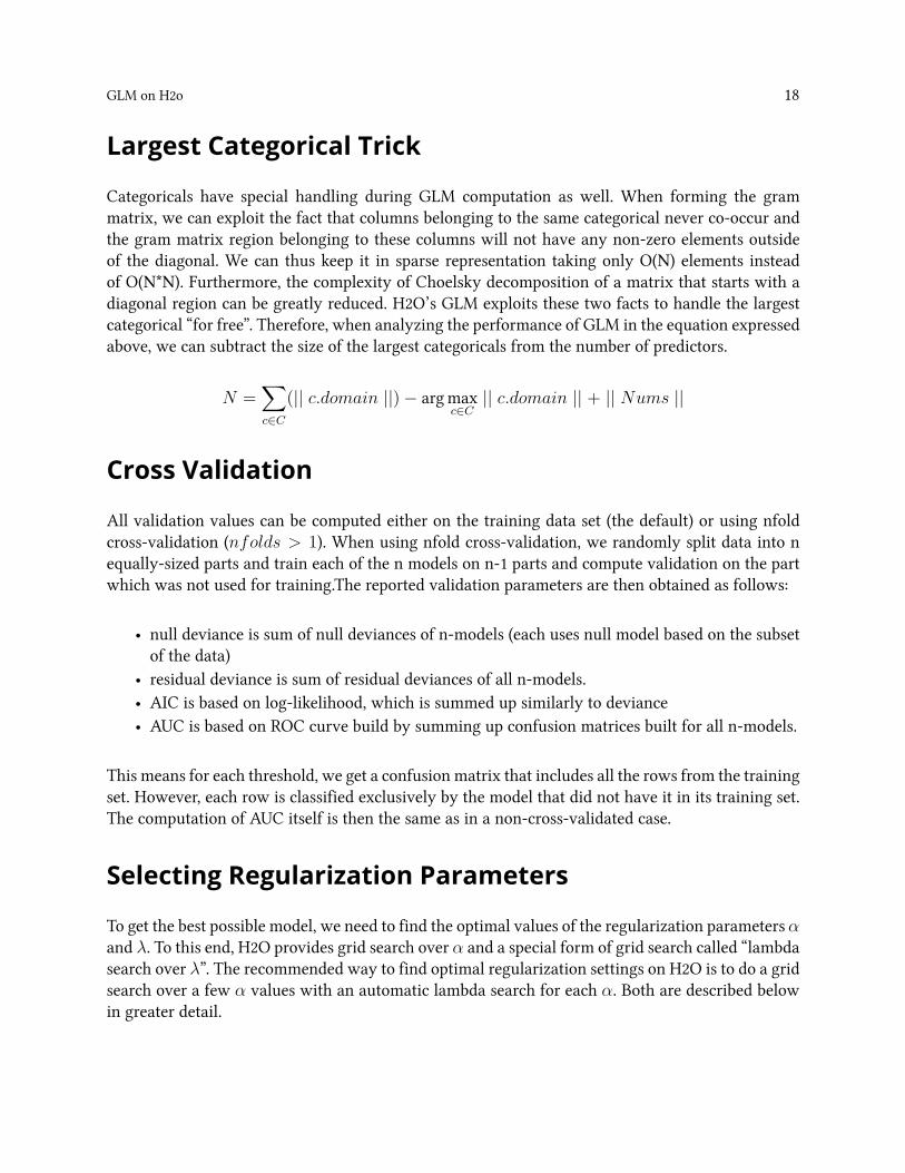
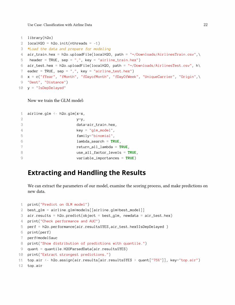
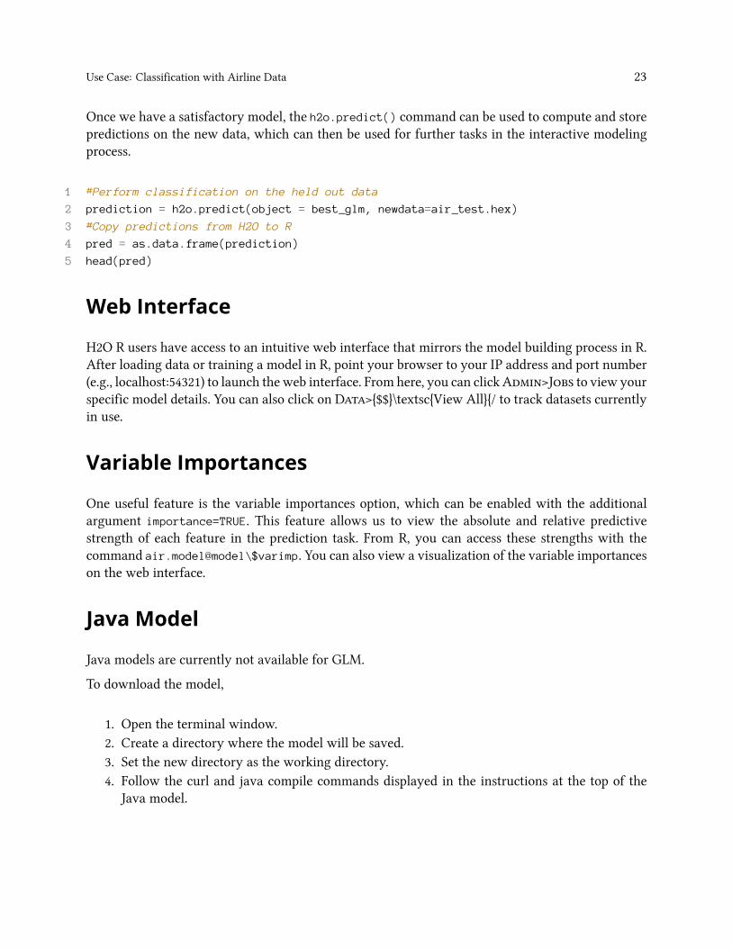
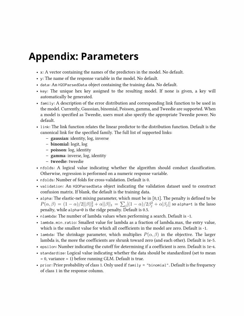
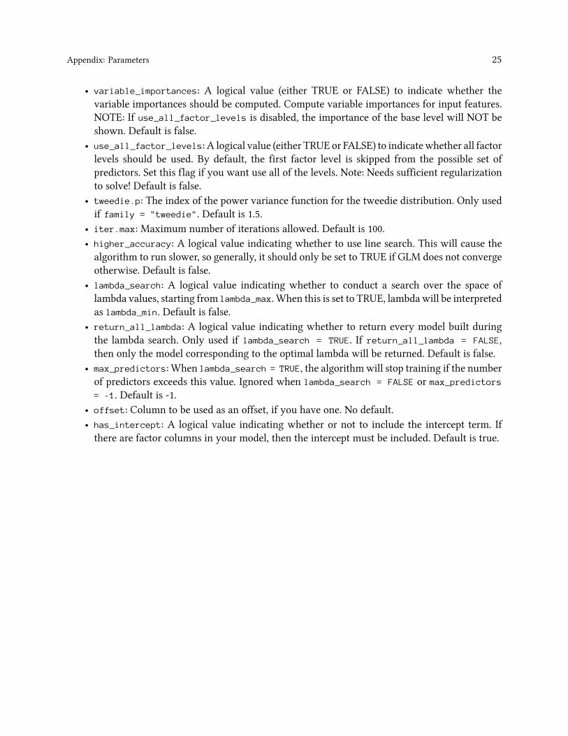