Glia-Augmented Arti cial Neural Networks: Foundations and ... · third section provides arti cial...
74
Glia-Augmented Artificial Neural Networks: Foundations and Applications by c ⃝ Zahra Sajedinia A thesis submitted to the School of Graduate Studies in partial fulfilment of the requirements for the degree of Master of Computer Science Department of Computer Science Memorial University of Newfoundland May 2015 St. John’s Newfoundland
Transcript of Glia-Augmented Arti cial Neural Networks: Foundations and ... · third section provides arti cial...

Glia-Augmented Artificial Neural Networks:
Foundations and Applications
by
c⃝ Zahra Sajedinia
A thesis submitted to the
School of Graduate Studies
in partial fulfilment of the
requirements for the degree of
Master of Computer Science
Department of Computer Science
Memorial University of Newfoundland
May 2015
St. John’s Newfoundland
Abstract
Information processing in the human brain has always been considered as a source
of inspiration in Artificial Intelligence; in particular, it has led researchers to develop
different tools such as artificial neural networks. Recent findings in Neurophysiology
provide evidence that not only neurons but also isolated and networks of astrocytes
are responsible for processing information in the human brain. Artificial neural net-
works (ANNs) model neuron-neuron communications. Artificial neuron-glia networks
(ANGN), in addition to neuron-neuron communications, model neuron-astrocyte con-
nections. In continuation of the research on ANGNs, first we propose, and evaluate a
model of adaptive neuro fuzzy inference systems augmented with artificial astrocytes.
Then, we propose a model of ANGNs that captures the communications of astrocytes
in the brain; in this model, a network of artificial astrocytes are implemented on top
of a typical neural network. The results of the implementation of both networks show
that on certain combinations of parameter values specifying astrocytes and their con-
nections, the new networks outperform typical neural networks. This research opens
a range of possibilities for future work on designing more powerful architectures of
artificial neural networks that are based on more realistic models of the human brain.
ii

Acknowledgements
Foremost, I would like to express my sincere gratitude to my supervisor Dr. Todd
Wareham for the continuous support of my masters study research and also providing
me with many curricular and extracurricular opportunities, and also for his patience,
motivation, and enthusiasm. I have learned so many things from him and I am truly
blessed to have him as my supervisor. This thesis definitely would not have been
possible without his encouragement and guidance. In one sentence I can say that I
could not have imagined having a better supervisor. Also, I would like to thank Dr.
Iris van Rooij, for her guidance, patience and encouragement; Her guidance helped
me in all the time of my study.
Also, I would like to thank Dr. Antonina Kolokolova for her support and thought-
ful comments specifically during departmental cognitive and neuroscience talks, her
encouragement and insightful comments always motivated me in continuing my re-
search. Also, I’d like to thank her for her helpful suggestions on the relation between
noise and astrocytes. Also, my gratitude extended to Dr. Siwei Lu, for introduc-
ing me to artificial neural networks and providing me with the opportunity to start
working on artificial glia networks. Furthermore I would also like to acknowledge
with much appreciation Ms Darlene Oliver, Brenda Hillier, and Sharon Deir at the
Computer Science general office.
Last but not the least, I would like to thank my family and friends, specifically my
parents Mohamad Sajedinia and Nahid Pahlavan for their endless love and support,
though no words can begin to express my heartfelt thanks for their kindness and
thoughtfulness.
iii
Contents
Abstract ii
Acknowledgements iii
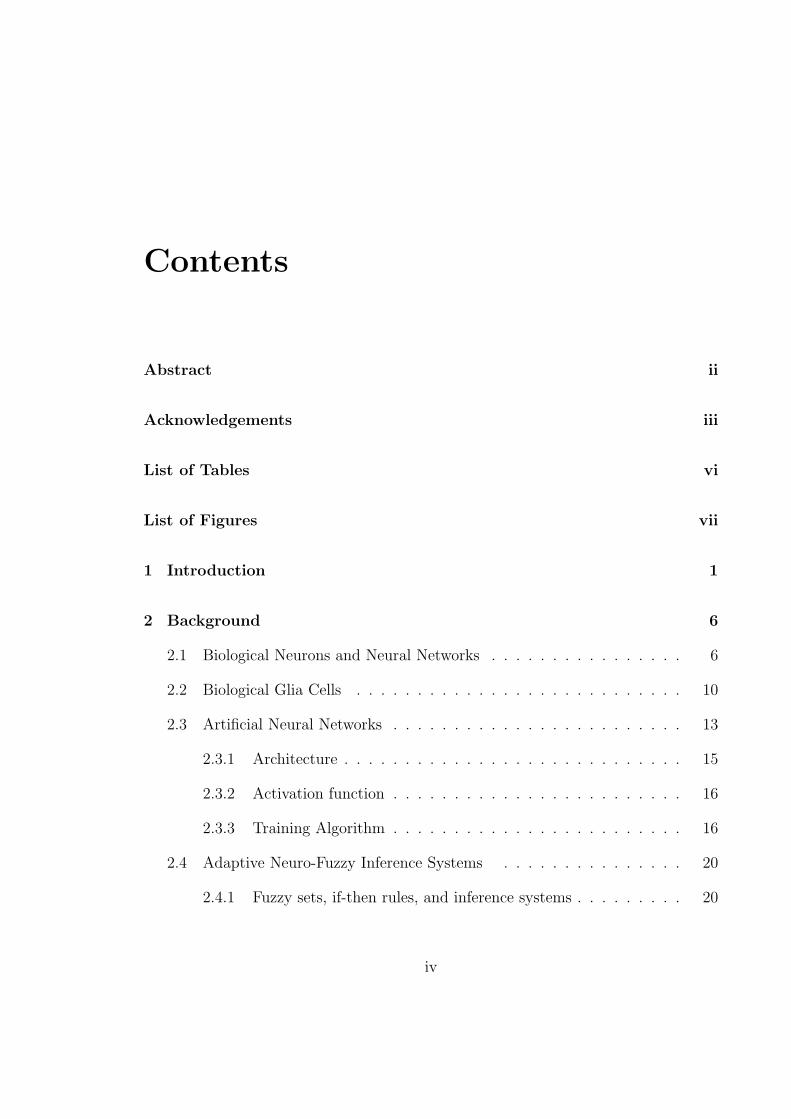
List of Tables vi
List of Figures vii
1 Introduction 1
2 Background 6
2.1 Biological Neurons and Neural Networks . . . . . . . . . . . . . . . . 6
2.2 Biological Glia Cells . . . . . . . . . . . . . . . . . . . . . . . . . . . 10
2.3 Artificial Neural Networks . . . . . . . . . . . . . . . . . . . . . . . . 13
2.3.1 Architecture . . . . . . . . . . . . . . . . . . . . . . . . . . . . 15
2.3.2 Activation function . . . . . . . . . . . . . . . . . . . . . . . . 16
2.3.3 Training Algorithm . . . . . . . . . . . . . . . . . . . . . . . . 16
2.4 Adaptive Neuro-Fuzzy Inference Systems . . . . . . . . . . . . . . . 20
2.4.1 Fuzzy sets, if-then rules, and inference systems . . . . . . . . . 20
iv

2.4.2 ANFIS architecture and algorithms . . . . . . . . . . . . . . . 22
2.5 Artificial Neuron-Glia Networks . . . . . . . . . . . . . . . . . . . . . 28
3 Adaptive Neuro-glia Fuzzy Inference System (ANGFIS) 33
3.1 Architecture and Learning Algorithm . . . . . . . . . . . . . . . . . . 34
3.1.1 Architecture . . . . . . . . . . . . . . . . . . . . . . . . . . . . 34
3.1.2 Learning Algorithm . . . . . . . . . . . . . . . . . . . . . . . . 34
3.2 Performance . . . . . . . . . . . . . . . . . . . . . . . . . . . . . . . . 36
3.3 Discussion . . . . . . . . . . . . . . . . . . . . . . . . . . . . . . . . . 40
4 Artificial Astrocytes Networks (AANs) 42
4.1 Architecture and Learning Algorithm . . . . . . . . . . . . . . . . . . 43
4.1.1 Architecture . . . . . . . . . . . . . . . . . . . . . . . . . . . . 43
4.1.2 Learning Algorithm . . . . . . . . . . . . . . . . . . . . . . . . 45
4.2 Performance . . . . . . . . . . . . . . . . . . . . . . . . . . . . . . . . 46
4.3 Discussion . . . . . . . . . . . . . . . . . . . . . . . . . . . . . . . . . 50
5 Summary and Future Work 54
5.1 Summary . . . . . . . . . . . . . . . . . . . . . . . . . . . . . . . . . 54
5.2 Future Work . . . . . . . . . . . . . . . . . . . . . . . . . . . . . . . . 55
Bibliography 58
v
List of Tables
3.1 Astrocyte parameters used for implementing ANGFIS . . . . . . . . . 39
3.2 The RMSE error for ANGFIS and ANFIS . . . . . . . . . . . . . . . 40
4.1 Parameters used in implementing ANGN and AAN . . . . . . . . . . 50
4.2 The accuracy of classification on test data for ANN, ANGN and AAN 50
vi

List of Figures
1.1 Biological neuron, artificial neuron, biological synapse and ANN synapses 2
1.2 A representation of a tripartite synapse . . . . . . . . . . . . . . . . . 4
2.1 A biological neuron . . . . . . . . . . . . . . . . . . . . . . . . . . . . 7
2.2 A biological synapse . . . . . . . . . . . . . . . . . . . . . . . . . . . 8
2.3 Transmission of a signal through a synapse . . . . . . . . . . . . . . . 10
2.4 Neurons and astrocytes in the brain . . . . . . . . . . . . . . . . . . . 11
2.5 Tripartite synapse . . . . . . . . . . . . . . . . . . . . . . . . . . . . . 12
2.6 Connections between astrocytes in the brain . . . . . . . . . . . . . . 13
2.7 An example of an artificial neural network . . . . . . . . . . . . . . . 14
2.8 Components of a Fuzzy Inference System . . . . . . . . . . . . . . . . 23
2.9 ANFIS Architecture . . . . . . . . . . . . . . . . . . . . . . . . . . . 24
2.10 An example of an Artificial Neuron-glia Network . . . . . . . . . . . . 29
2.11 An artificial neuron and its associated astrocyte . . . . . . . . . . . . 32
3.1 Architecture of an ANGFIS . . . . . . . . . . . . . . . . . . . . . . . 35
4.1 ANGN and AAN . . . . . . . . . . . . . . . . . . . . . . . . . . . . . 44
4.2 A flowchart of the AAN algorithm . . . . . . . . . . . . . . . . . . . . 47
vii
Chapter 1
Introduction
The human brain has always been considered as a source of inspiration in develop-
ing tools and algorithms in computer science. The human brain seems to have an
advantage in solving problems where no explicit rules are given [5]. To benefit from
this characteristic of the brain, researchers developed computational tools that mimic
the way the human brain works. Artificial neural networks (ANNs) are one of these
computational tools which for representing biological neural systems. They are capa-
ble of learning from experience [12]. Currently, ANNs are used in different fields of
science from business to medicine and robotics [11].
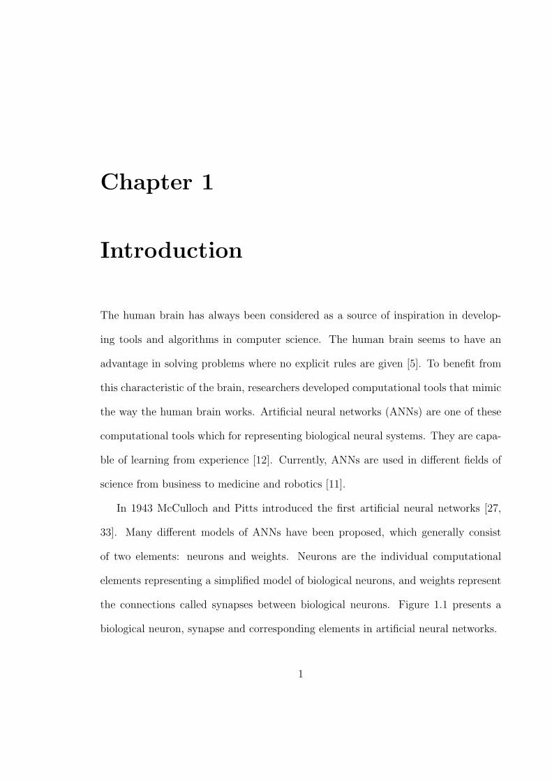
In 1943 McCulloch and Pitts introduced the first artificial neural networks [27,
33]. Many different models of ANNs have been proposed, which generally consist
of two elements: neurons and weights. Neurons are the individual computational
elements representing a simplified model of biological neurons, and weights represent
the connections called synapses between biological neurons. Figure 1.1 presents a
biological neuron, synapse and corresponding elements in artificial neural networks.
1
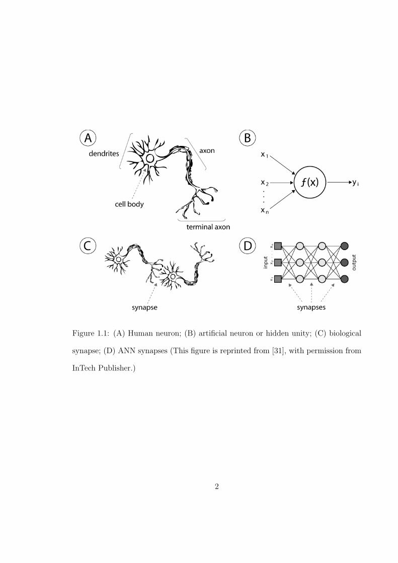
Figure 1.1: (A) Human neuron; (B) artificial neuron or hidden unity; (C) biological
synapse; (D) ANN synapses (This figure is reprinted from [31], with permission from
InTech Publisher.)
2

Although the human brain consists of neurons and glia cells, ANNs generally
represent only neurons. It is estimated that there are 10 to 50 times more glia cells
than there are neurons in the brain [16]. Recent discoveries in neuroscience show that
glia cells, in addition to doing passive functions such as providing nutrition for neurons
and collecting wastes from neurons, modulate synapses and process information [64,
49]. In more detail, the process by which glia cells modulate synapses begins with
the release of neurotransmitters from a pre-synaptic neuron; this release then evokes
an increase in calcium ions in neighbouring glia cells. Glia cell in response release
transmitters. These transmitters will reach pre-synaptic and post-synaptic neurons
and enhance or depress further release of neurotransmitters. Therefore, glia cells
regulate synaptic transmissions and as a result they affect information processing
[39].
Presently, the concept of tripartite synapse is well known in neurophysiology,
which states that each synapse consists of three parts: presynaptic elements, post-
synaptic elements, and surrounding astrocytes (see Figure 1.2).
Neurons and astrocytes internally transfer information in different ways. Neurons
mainly transfer electrical signals; and astrocytes propagate information by chemical
waves. [42, 4, 3, 44, 45, 48, 46, 47, 6, 55, 17].
Inspired by the way in which glia astrocytes modulate synapses, researchers have
developed a novel type of neural network called an artificial neuron-glia network
(ANGN) [52, 1]. In ANGNs, each neuron is connected to one astrocyte cell, and
activation (inactivation) of the neuron for a specific period of time will make the
connected astrocyte active; as a result, the connected weights will be increased (or
decreased) by a pre-defined factor [1]. Chapter 2 provides greater details on the
3
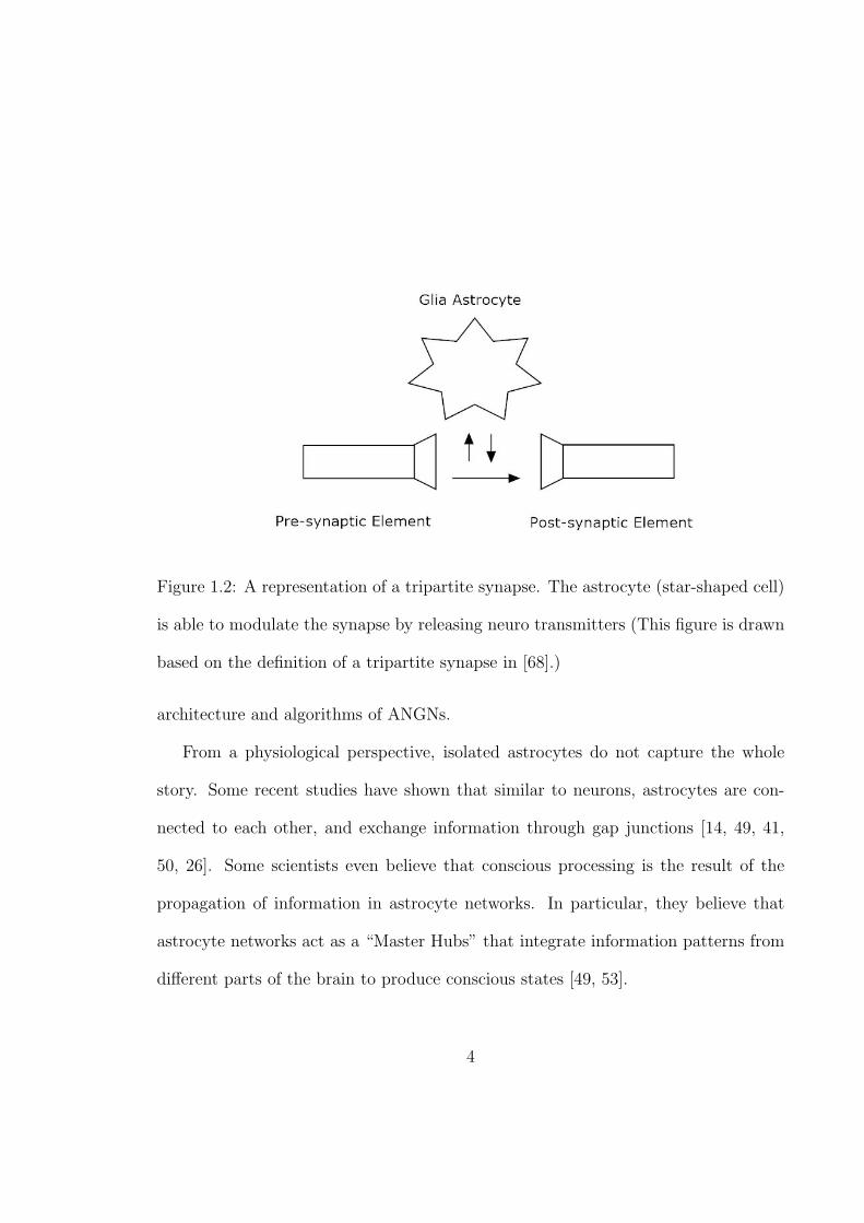
Figure 1.2: A representation of a tripartite synapse. The astrocyte (star-shaped cell)
is able to modulate the synapse by releasing neuro transmitters (This figure is drawn
based on the definition of a tripartite synapse in [68].)
architecture and algorithms of ANGNs.
From a physiological perspective, isolated astrocytes do not capture the whole
story. Some recent studies have shown that similar to neurons, astrocytes are con-
nected to each other, and exchange information through gap junctions [14, 49, 41,
50, 26]. Some scientists even believe that conscious processing is the result of the
propagation of information in astrocyte networks. In particular, they believe that
astrocyte networks act as a “Master Hubs” that integrate information patterns from
different parts of the brain to produce conscious states [49, 53].
4

In continuation of published research on neuron-glia networks, we have done two
separate implementations. Firstly, we combine ANGNs with adaptive neuro fuzzy
inference systems (ANFIS). We investigate the performance of ANFIS on two sample
problems with and without astrocytes. The results show a decrease of the overall error
in the systems that contain astrocytes. Secondly, we design a new type of ANGNs
in which artificial astrocyte networks (AANs) are connected to neurons rather than
single isolated astrocytes. The networks of astrocytes are implemented on top of a
multi-layer back propagation ANN, and the resulting network is tested for classifying
two data sets. The results show that having an attached network of astrocytes on
top of a typical neural network improves the performance.
This thesis is organized as follows. Chapter 2 provides some background informa-
tion on physiological and artificial neurons, glia cells, neural and glia networks, and
fuzzy inference systems. Chapter 3 introduces and evaluates the proposed system of
adaptive neuro-glia fuzzy inference system (ANGFIS). Chapter 4 presents the new
concept of artificial astrocyte networks (AANs), and evaluates the performance of
this network in comparison to other types of artificial neural networks. Note that
the material in Chapters 3 and 4 is partially published as [57], and [56]. Finally,
Chapter 5 presents a summary of the research presented in this thesis and discusses
some possible directions for future work.
5

Chapter 2
Background
This chapter is divided into five sections. Each section provides an introductory
overview of a topic addressed in this thesis. The first section presents biological
neurons and neural networks; the second section introduces biological glia cells; The
third section provides artificial neural network, and the forth and fifth sections in-
troduce adaptive neuro fuzzy inference systems and artificial neuron-glia networks
respectively.
2.1 Biological Neurons and Neural Networks
The human brain is considered as one of the most complex systems in the universe
[59]. Despite tremendous efforts to understand the mechanisms that underlie the
brain’s architecture and processes, many aspects are still poorly understood [43].
However, some fundamental information about the brain, such as the structure and
functions of neurons and synapses have been discovered by neuroscientists in the last
two centuries. This information has helped researchers to make simplified models of
6

Figure 2.1: A biological neuron. The three main parts of the neuron (dendrites,
soma, and axon), nucleus of the neuron, myelin sheath (yellow) that speeds up the
electrical signals, and the axon’s terminal buttons can be seen in the figure (This
figure is released under the GNU Free Documentation License.)
the brain [40].
Neurons or nerve cells are the basic building blocks of the brain. Neurons conduct
electrical impulses, which result in processing information. As shown in Figure 2.1,
a biological neuron consists of three main parts: dendrites, soma, and axon:
• Dendrites are considered as the inputs of a neuron1 They receive electrical
signals from other neurons and send them to the soma [43, 11, 5].
• Soma or cell body receives signals from dendrites. If the electrical charge pro-
1In modern Neuroscience, dendrites are shown to be more than an input channel [8]. However,
in this thesis, we only consider the ‘input’ characteristic of dendrites to remain consistent with the
definition of artificial neural networks [11].
7
Figure 2.2: A biological synapse. A synapse is a junction between two neurons,
consisting of a gap across which impulses pass by diffusion of neurotransmitters (This
figure is reprinted from NIH, with permission from the publisher.)
8

duced by the received signals is sufficient, then the neuron fires; this means
that the neuron sends a signal through its axon to all of the connected neurons.
Most often, it is supposed that in any instant of time, a neuron either fires or
not. This characteristic makes it possible to look at the output of a neuron as a
binary function (fired or not fired.) However, in reality, the frequency of firing
is different and can be seen as a signal of either greater or lesser magnitude.
This corresponds to looking at discrete time steps and accumulating all of the
activity (signal received or signals sent) at a particular point in time [11].
• Axons are the output units2. They transfer the firing signal from the soma
to neurons connected to axon terminals. Unlike dendrites, which are many
short branches connected to a neuron’s soma, neurons have only one axon that
connects soma to other neurons. It should be mentioned that an axon may
branch hundreds of times before it terminates. The transmission of a signal is
completed by an action potential resulting from differential concentrations of
ions, such as potassium, sodium and chloride on either side of an axon [43, 11].
A single neuron may be connected to many other neurons. The connections are
made through synapses. Figure 2.2 shows a synapse. Communication between neu-
rons is the result of the release of chemicals called neurotransmitters. The pre-synaptic
neuron release neurotransmitters and the post-synaptic neuron subsequently absorbs
these neurotransmitters [11, 43]. The process begins by the movement of an action
potential through the axon from the pre-synaptic soma to its membrane, which is
2Similar to dendrites, axons can serve more as output channels; signals can reach the soma from
the neuron’s axon [65]. However, in order to be consistent with the assumptions in artificial neural
networks [11], in this thesis, we consider axons only as output units.
9

Figure 2.3: Transmission of a signal through a synapse (This figure is reprinted from
[66], with permission from the publisher.)
located at the axon’s terminal buttons. When the action potential arrives at the pre-
synaptic membrane, it changes the permeability of the membrane and causes an influx
of calcium ions. These calcium ions cause the vesicles containing neurotransmitters
to fuse with the pre-synaptic membrane, resulting in the release of neurotransmitters
into the synaptic cleft. If the receptors of the post-synaptic neuron receive enough
neurotransmitters, an electrical signal will be sent through the dendrites of the post-
synaptic neuron [43]. This process is illustrated in Figure 2.3.
2.2 Biological Glia Cells
The human brain consists of two main types of cells, neurons and glia cells. It is
estimated that there are 10 to 50 times more glia cells than there are neurons in the
brain [16]. Figure 2.4 shows a portion of the brain in which both neurons and glia
10

cells can be seen. Until two decades ago, it was widely believed that glia cells only
performed passive functions and did not interfere with processing information [49].
New evidence supports the conception that a specific type of glia cells named
astrocytes3 affect learning by modulating synapses. This has led to a new concept in
neurophysiology, the tripartite synapse, which consists of three parts: pre-synaptic
elements, post-synaptic elements, and surrounding astrocytes (Figure 2.5.) While
neurons communicate by electrical signals, astrocytes use chemicals for propagating
information; therefore, astrocytes are slower than neurons in processing information
[42, 4, 3, 44, 45, 48, 46, 47, 6, 55, 17].
Figure 2.4: Neurons (green) and glia cells (red) in the brain (This figure is reprinted
from Image: IN Cell Image Competition ( c⃝ GE Healthcare - All rights reserved.),
with permission from the publisher.)
Recent studies suggest that not only neurons, but also astrocytes are connected
into networks. While neurons exchange information through synapses, gap junctions
3Astrocytes are also known as glia astrocytes. In this thesis we refer to this type of cells as
astrocytes.
11

Figure 2.5: Tripartite synapse. The astrocyte is able to modulate the synapse by
releasing transmitters (This figure is reprinted from [68], with permission from the
publisher.)
are the path of communication for astrocytes [14, 49, 41, 50, 26]; however, the exact
connections between astrocytes is not completely elucidated. Some other studies have
taken a further step and assigned integration of data from different parts of the brain
(which is in turn hypothesized to underlie conscious processing) to astrocyte networks
[49, 53]. Pereira, Jr. and Furlan in their 2010 paper stated that
“the division of work in the brain is such that the astrocyte network conveys the
feeling, while neural networks carry information about what happens.”
They believe consciousness is the result of integration of data by means of wavelike
computing in the astrocytic networks [49]. Figure 2.6 illustrates connections between
glia astrocyte in the human brain.
12

Figure 2.6: Connections between astrocytes in the brain (This figure is reprinted
from Synapse Web, Kristen M. Harris, PI, http://synapses.clm.utexas.edu/, with
permission from the publisher.)
2.3 Artificial Neural Networks
Artificial neural networks or AANs are information processing systems that are in-
spired by biological neural networks [11]. From 1943 when McCulloch and Pitts
introduced the first simple ANNs until the present time, many different types of
ANNs have been proposed. They are applied in solving problems in different fields,
such as risk assessment, optimization, and pattern recognition [43]. Most AANs are
designed based on the following assumptions [11]:
• Simple elements called neurons are responsible for processing information.
• The connections between neurons provide the possibility of transferring signals
from one neuron to another.
• Each connection has an associated weight, which strengthens or weakens the
transferred signal.
13
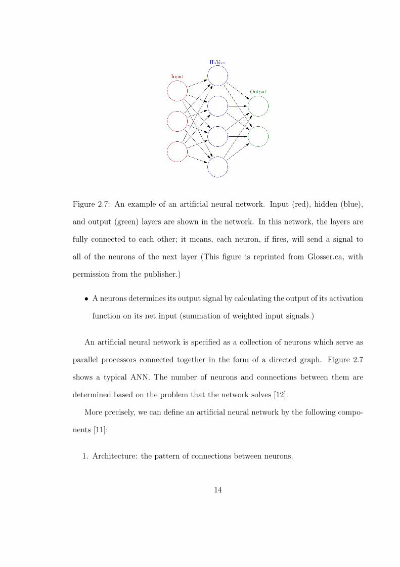
Figure 2.7: An example of an artificial neural network. Input (red), hidden (blue),
and output (green) layers are shown in the network. In this network, the layers are
fully connected to each other; it means, each neuron, if fires, will send a signal to
all of the neurons of the next layer (This figure is reprinted from Glosser.ca, with
permission from the publisher.)
• A neurons determines its output signal by calculating the output of its activation
function on its net input (summation of weighted input signals.)
An artificial neural network is specified as a collection of neurons which serve as
parallel processors connected together in the form of a directed graph. Figure 2.7
shows a typical ANN. The number of neurons and connections between them are
determined based on the problem that the network solves [12].
More precisely, we can define an artificial neural network by the following compo-
nents [11]:
1. Architecture: the pattern of connections between neurons.
14

2. Activation function: the function that determines the output of a neuron based
on its net input.
3. Learning or training algorithm: a method that determines how to change the
weights on the connections.
Each of these components is described in more details below:
2.3.1 Architecture
For designing an ANN’s architecture, it is more convenient to arrange neurons into
layers. Most neural networks have an input layer. Each neuron in the input layer
receives an external input signal, and send it to the connected neurons. If we have
only two layers, input and output, then the network is called a single-layer net [12, 11].
Usually, single-layer nets can solve relatively less complicated problems in comparison
to multi-layer networks. Multi-layer networks have one or more layers between input
and output layer, named hidden layers. These networks have the ability to save
important information in the weights connected to hidden layers, and use them in
solving more complicated problems; however training is more difficult in multi-layer
networks rather than the single-layer nets [11]. The connections between neurons can
be feed-forward or recurrent. In feed-forward nets the signal flows from the first layer
to the last layer in a forward direction. However, in recurrent nets, the signals from a
neuron can come back to itself or to the neurons in the same or earlier layers, allowing
the connections in the network to make closed loops [11].
15
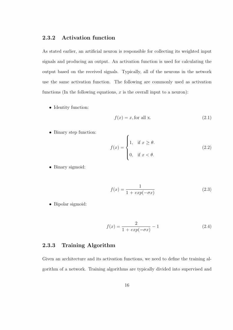
2.3.2 Activation function
As stated earlier, an artificial neuron is responsible for collecting its weighted input
signals and producing an output. An activation function is used for calculating the
output based on the received signals. Typically, all of the neurons in the network
use the same activation function. The following are commonly used as activation
functions (In the following equations, x is the overall input to a neuron):
• Identity function:
f(x) = x, for all x. (2.1)
• Binary step function:
f(x) =
1, if x ≥ θ.
0, if x < θ.
(2.2)
• Binary sigmoid:
f(x) =1
1 + exp(−σx)(2.3)
• Bipolar sigmoid:
f(x) =2
1 + exp(−σx)− 1 (2.4)
2.3.3 Training Algorithm
Given an architecture and its activation functions, we need to define the training al-
gorithm of a network. Training algorithms are typically divided into supervised and
16
unsupervised algorithms4. In supervised training, a sequence of training vectors, or
patterns with an associated target vectors is presented to the ANN [11]. Presenting
a training vector will produce an output vector, and based on the difference between
these output and the associated target vector, an error will be calculated and the
weights will be modified in a way to reduce the error. Backpropagation is a well-
known supervised algorithm [43, 11, 5]. In unsupervised training, we do not need a
training session prior to using the network because in some cases we do not know of
the response we should expect from the neural network. The neural network reorga-
nizes itself to decides what output is best for a given input. There are two main types
of unsupervised learning, reinforcement and competitive learning. In reinforcement
learning, the network tries to modify the weights in order to produce the maximum
reproduction of the output. Hebbian learning is one of the well-know reinforcement
algorithms, which is explained in more detail at the following paragraph. In competi-
tive learning, the neurons compete with each other by increasing and decreasing their
weights until finally one node wins and this node will represent the answer [11, 54].
Hebb’s rule (see Algorithm 1) is a physiology-based theory proposed by Donald
Hebb in 1949. It describes how learning happens in neural networks, and provides an
algorithm to update weight of neuronal connections within a neural network. It states
that the weights connections between neurons is a function of neuronal activity [28].
This means that if a pre-synaptic neuron repeatedly sends a signal to a post-synaptic
neuron, then the synapse between these neurons will become stronger and increase
the strength of the signal in future transmissions. Mathematically, this is shown in
4There are training algorithms which are neither supervised nor unsupervised [11], but in this
thesis, these types of algorithms are not considered.
17

Equation 2.5 in Algorithm 1 [43, 11, 5].
In backpropagation algorithm (see Algorithm 2), the term “backpropagation” is
an abbreviation for “backward propagation of errors.” Backpropagation consists of
two phases, forward and backward propagation. In the forward propagation phase,
the training input propagates through the network and generates an output. In the
backward propagation phase, the difference (delta) between the current output and
the desired output is determined. Then, for each weight, the gradient of the weights,
which is the multiplication of the delta and input activation, is calculated. Finally, a
ratio of the gradient will be subtracted from the current weights. This ratio, which is
called the learning rate, determines the speed and accuracy of training. Usually, the
learning rate is a number between 0 and 1 [43, 11, 5].
Algorithm 1 Hebb Training AlgorithmInput
• xj: the output of the pre-synaptic neuron.
• xi: the output of the post-synaptic neuron.
• α: The learning rate, which adjusts the speed of learning.
Weight modification after each iteration
∆Wij(t) = αxjxi (2.5)
where ∆Wij(t) is the change in the weight of the synapse between neurons i and
j at iteration t.
18

Algorithm 2 Backpropagation learning algorithm.
The activation function is assumed to be a sigmoid function.
Initialize all weights to small random numbers.
Until the error is less than a threshold, Do
for each training example do
Forward Pass
Input the training example to the network and compute the network output.
Backward Pass: Calculate the error of Output Units
For each output unit k:
δk = ok(1− ok)(tk − oK) (2.6)
where ok is the output, and tk is the desired output for neuron k
Backward Pass: Calculate the error of hidden Units
For each hidden unit h:
δh = oh(1− oh)(∑k
whkδk) (2.7)
where oh is the output of neuron h
Backward Pass: Update each weight wij:
For each neuron:
∆Wij = αδjxi (2.8)
where Wij represents the weight between neuron i and j, and α
is the learning rate, and xi is the input of the neuron i.
end for
19

2.4 Adaptive Neuro-Fuzzy Inference Systems
Conventional mathematical tools such as differential equations are not always bene-
ficial in modeling uncertain or ill-defined problems. For this reason, tools like fuzzy
inference systems have been designed to implement qualitative knowledge rather than
precise quantitative analyses. Adaptive Neuro-fuzzy Inference Systems (ANFIS) are
a specific type of fuzzy inference systems that are able to adjust their own parameters
in order to generate the stipulated input-output pairs [21]. In the reminder of this
section, first we introduce fuzzy sets, fuzzy if-then rules and fuzzy inference systems,
and then we present the architecture and algorithms of ANFIS.
2.4.1 Fuzzy sets, if-then rules, and inference systems
In the classical set theory, the membership is defined precisely, an object is either
belongs or does not belong to a set; However, in reality the classes of object might or
might not precisely define criteria of membership; for example, we can clearly define
the class of real numbers which are greater than 1 but we cannot precisely define
the class of tall people. The human thinking process uses imprecise definitions of
classes to recognize patterns, communicate and do abstraction [72, 73]. Introduced
by Zadeh in 1965, fuzzy sets were to model these imprecise definitions. The objects
in a fuzzy set are described by a continuum of grades of membership. These grades of
membership are numbers between 0 and 1, and they are assigned by the membership
function of the fuzzy set [72].
A more formal definition of fuzzy sets, which is presented by Zadeh in [72, p. 339]:
“Let X be a space of objects, with a generic element of X denoted
20
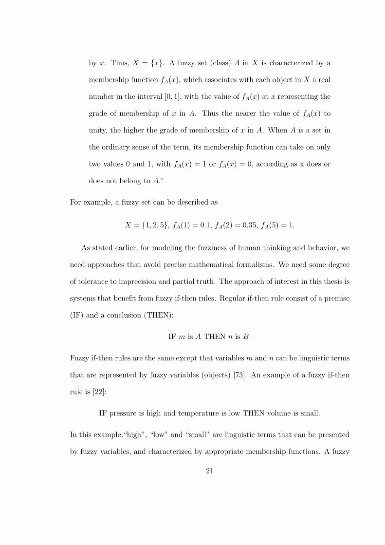
by x. Thus, X = {x}. A fuzzy set (class) A in X is characterized by a
membership function fA(x), which associates with each object in X a real
number in the interval [0, 1], with the value of fA(x) at x representing the
grade of membership of x in A. Thus the nearer the value of fA(x) to
unity, the higher the grade of membership of x in A. When A is a set in
the ordinary sense of the term, its membership function can take on only
two values 0 and 1, with fA(x) = 1 or fA(x) = 0, according as x does or
does not belong to A.”
For example, a fuzzy set can be described as
X = {1, 2, 5}, fA(1) = 0.1, fA(2) = 0.35, fA(5) = 1.
As stated earlier, for modeling the fuzziness of human thinking and behavior, we
need approaches that avoid precise mathematical formalisms. We need some degree
of tolerance to imprecision and partial truth. The approach of interest in this thesis is
systems that benefit from fuzzy if-then rules. Regular if-then rule consist of a premise
(IF) and a conclusion (THEN):
IF m is A THEN n is B.
Fuzzy if-then rules are the same except that variables m and n can be linguistic terms
that are represented by fuzzy variables (objects) [73]. An example of a fuzzy if-then
rule is [22]:
IF pressure is high and temperature is low THEN volume is small.
In this example,“high”, “low” and “small” are linguistic terms that can be presented
by fuzzy variables, and characterized by appropriate membership functions. A fuzzy
21

if-then rule that only allows the premise to involve fuzzy sets is called Takagi and
Sugeno fuzzy if-then rule [62, 21].
A system that applies fuzzy if-then rules is known as a fuzzy inference system. A
fuzzy inference system is composed of five functional units [21]:
1. Rule base unit, which consists of fuzzy if-then rules;
2. Database unit, which defines the membership function;
3. Decision-making unit, which applies the inference operations on the rules;
4. Fuzzification unit, which transforms the crisp inputs into linguistic terms (fuzzy
variables); and
5. Defuzzification unit, which transforms the fuzzy results into crisp output.
Figure 2.8 illustrates the components of a fuzzy inference system.
A fuzzy inference system starts with fuzzifying the crisp inputs into membership
degrees. The next unit, decision maker, evaluates the fuzzified inputs to determine
the strength of the rule’s “If” parts, and infers the consequences of the rules. The
final part, the defuzzification unit, transform the fuzzy results into crisp data.
2.4.2 ANFIS architecture and algorithms
An ANFIS which can stand for Adaptive Network-Based Fuzzy Inference System [21]
or Adaptive Neuro-Fuzzy Inference System [15], is a fuzzy inference system that ap-
plies ANNs to data samples to determine properties of these samples [15, 21, 22]. In
22
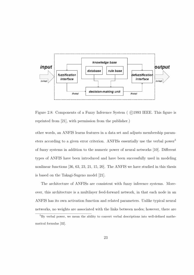
Figure 2.8: Components of a Fuzzy Inference System ( c⃝1993 IEEE. This figure is
reprinted from [21], with permission from the publisher.)
other words, an ANFIS learns features in a data set and adjusts membership param-
eters according to a given error criterion. ANFISs essentially use the verbal power5
of fuzzy systems in addition to the numeric power of neural networks [10]. Different
types of ANFIS have been introduced and have been successfully used in modeling
nonlinear functions [36, 63, 23, 21, 15, 20]. The ANFIS we have studied in this thesis
is based on the Takagi-Sugeno model [21].
The architecture of ANFISs are consistent with fuzzy inference systems. More-
over, this architecture is a multilayer feed-forward network, in that each node in an
ANFIS has its own activation function and related parameters. Unlike typical neural
networks, no weights are associated with the links between nodes; however, there are
5By verbal power, we mean the ability to convert verbal descriptions into well-defined mathe-
matical formulas [32].
23

Figure 2.9: ANFIS Architecture (This figure is adapted from [13], with permission
from InTech publisher.)
parameters associated with some nodes in an ANFIS that have a similar role to the
weights of typical neural networks. These parameters are modified during training to
reduce the total error.
Figure 2.9 illustrates the architecture of an ANFIS. Layers 1 and 5 perform fuzzifi-
cation and defuzzification respectively, and rest of the layers implement fuzzy if-then
rules.
The steps of fuzzy reasoning performed by an ANFIS can be stated in four steps
24

[21, 22]:
1. Compare the input variables with the membership function on the premise part
to obtain the membership values (or compatibility measures) of each linguistic
label (this step is often called fuzzification;)
2. Combine (through a specific T-norm operator, usually multiplication or min-
imum.) the membership values on the premise part to get firing strength
(weights) of each rule;
3. Generate the qualified consequent (either fuzzy or crisp) of each rule depending
on the firing strength; and
4. Aggregate the qualified consequent to produce a crisp output (this step is called
defuzzification)
The following example provides a more detailed explanation on how the architec-
ture and algorithm of ANFIS works: assume we have one output f and two inputs
m and n; also, we have two Takagi and Sugeno fuzzy if-then rules:
• Rule 1: If (m is A1 and n is B1) then f1 = p1m+ q1n+ r1
• Rule 2: If (m is A2 and n is B2) then f2 = p2m+ q2n+ r2
where the parameters p1, p2, q1, q2, r1 and r2 are linear, and A1, A2, B1 and B2 are
nonlinear [30, 21].
To design an ANFIS corresponding to these parameters and rules, we need the
architecture shown in Figure 2.9. Similar to other ANFIS architectures, there are 5
layers.
25

• Layer 1 considers the “if” parts of the given if-then rules: “If m is A1 or A2”
and “If n is B1 and B2.” This layer receives m and n as input, and determines
to what degree m belongs to A1 and A2 and n belongs to B1 and B2. The
activation function of this layer can be expressed as:
O1i = µAi(m) for i ∈ 1, 2 (2.9)
O1j = µBj(n) for j ∈ 1, 2 (2.10)
where O1i is the output function for node Ai, O1j is the output function for
node Bj in layer 1, and µAiand µBj
denote the membership functions [30, 21].
• Informally, Layer 2 determines the strength of the “If” part by multiplying the
outputs of Layer 1. The number of nodes in Layer 2 and the links between Layer
1 and Layer 2 are determined by the rules. For example, Rule 1 presents “If
(m is A1 and n is B1)”; to implement this rule, we make links from A1 and B1
to the first node in Layer 2 (note that each node in Layer 2 represent a specific
rule, where the first node represents the first rule, and so on). To implement
“If (m is A2 and n is B2)” in Rule 2, we link A2 and B2 to the second node in
Layer 2. The activation function of the nodes in Layer 2 is as follows:
O2i = wi = µAi(m) ∗ µBi
(n) for i ∈ 1, 2 (2.11)
where, O2i denotes the output of Layer 2, node i [30, 21].
26
• The third layer normalizes the outputs from Layer 2. The activation function
of this layer is
O3i = wi =wi
w1 + w2
for i ∈ 1, 2 (2.12)
where, O3i denotes the output of node i in Layer 3 [30, 21].
• The fourth layer performs the “Then” part of the rules. The nodes in this layer
in addition to the outputs of Layer 3, receive the original inputs (m and n), and
then by applying the activation function on these parameters, produce their
results. The activation function in this layer uses three parameters, pi, qi, and
ri, and calculate the output as
O4,i = wifi = wi(pim+ qin+ ri) for i ∈ 1, 2 (2.13)
where, O4,i denotes the output of node i in Layer 4 [30, 21].
• Layer 5 is the output layer. It integrates the outputs from Layer 4. The acti-
vation function of this node is
O5 = Σiwifi =ΣiwifiΣiwi
(2.14)
where O5 denotes the output of the node in layer 5 [30, 21].
The learning algorithm of ANFISs is similar to the backpropagation algorithm
(see Section 2.3.3), in that there is a feed-forward flow of data followed by an up-
date of the parameters. For updating the parameters the followings formulas will be
used. Assume we have a training data set that has P elements. The overall error is
27

calculated as
E =
p∑p=1
Ep, (2.15)
where, Ep is the error for the pth (1 ≤ p ≤ P ) element in the data set is calculated as
Ep =
|L|∑m=1
(Tm,p −OLm,p)
2, (2.16)
where, Tm,p is the mth component of the pth desired output vector and OLm,p is the
mth component of actual output vector produced by presenting the pth input vector.
Given the above, each parameter in the network will be updated as
∆(param) = −αδE
δ(param), (2.17)
where param presents the parameter studied and α is the learning rate [30, 21].
2.5 Artificial Neuron-Glia Networks
Inspired by the concept of tri-partite synapse, Porto in 2004 developed a novel type
of neural networks called an Artificial Neuron-Glia Network (ANGN) [51]. It was
successfully implemented in different ANN architectures [56, 25, 1, 18], and success-
fully tested on real world problems [25, 52]. These tests showed that adding artificial
astrocytes to typical ANNs improves performance of the network, but the degree of
success is highly dependent on the complexity of the problem [52]. The architecture of
an ANGN can be described as an extension of a typical ANN. ANGNs include a novel
type of processing element, the artificial astrocyte, and each neuron is associated with
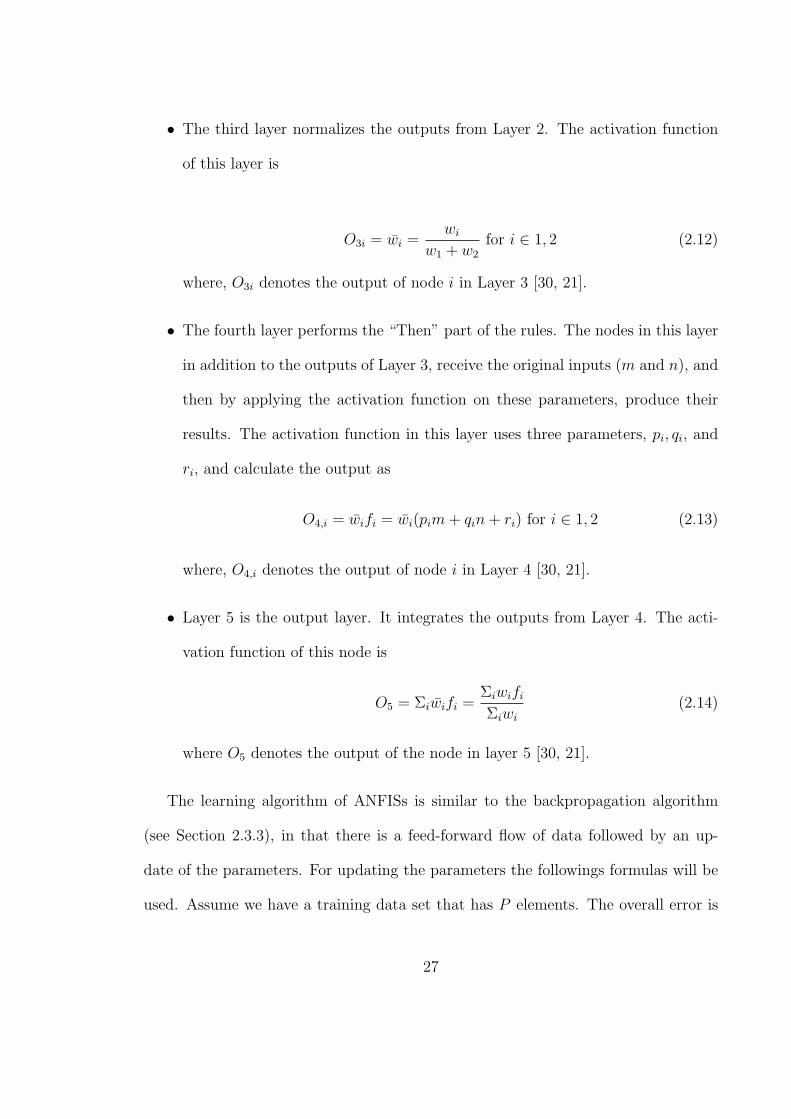
one astrocyte. Figure 2.10 shows the architecture of an ANGN.
28
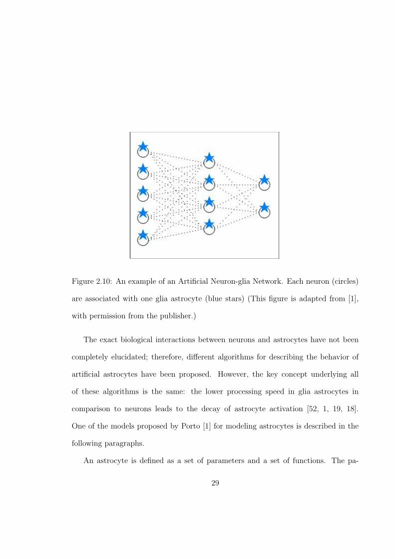
Figure 2.10: An example of an Artificial Neuron-glia Network. Each neuron (circles)
are associated with one glia astrocyte (blue stars) (This figure is adapted from [1],
with permission from the publisher.)
The exact biological interactions between neurons and astrocytes have not been
completely elucidated; therefore, different algorithms for describing the behavior of
artificial astrocytes have been proposed. However, the key concept underlying all
of these algorithms is the same: the lower processing speed in glia astrocytes in
comparison to neurons leads to the decay of astrocyte activation [52, 1, 19, 18].
One of the models proposed by Porto [1] for modeling astrocytes is described in the
following paragraphs.
An astrocyte is defined as a set of parameters and a set of functions. The pa-
29

rameters are k ∈ N\0, θ ∈ 1, ..., k, a, b ∈ [0, 1] and ft ∈ R. The activity of the
corresponding astrocyte to each neuron will be represented by the following func-
tions:
• U : R → Z, determines whether the corresponded neuron to the astrocyte is
fired or not, and is defined as follows:
U(x) =
−1, if x ≤ ft.
1, if x > ft.
(2.18)
where x is the output of the corresponding neuron, ft is the threshold of firing,
and the output of U indicates whether the neuron has fired (U(x) = 1) or not
(U(x) = −1).
• r : N → [−θ,+θ], where r represents how many times the neuron was fired in
the k consecutive cycles. The output of −θ or +θ results in the activation of
the astrocyte. −θ means that in the the k preceding cycles, the corresponded
neuron did not fire for θ times, and +θ represents the firing of the neuron for θ
times.
The associated weights of an active astrocytes6 will be modified as follows:
w(t+∆t) = w(t) + ∆w(t) (2.19)
where ∆w(t) is defined as
∆w(t) = |w(t)|z(t) (2.20)
6The associated weights of an astrocyte are the weights connecting the astrocyte’s associated
neuron and the neurons in the next layer.
30

and function z : N\0 → R indicates the percentage of the change of the weights
based on the astrocyte activation7. Figure 2.11 shows how an astrocyte can modify
the weights of a neuron.
7In this thesis, the output of the z function will be a if the astrocyte is positively activated and
b if it is negatively activated. In other words if output of the r function is greater than θ then the
output of z will be a, and if the output of the r function is less than θ then the output of z will be b.
31

Figure 2.11: An artificial neuron and its associated astrocyte (grey box). The output
of the neuron j, Oj is the input of its augmented glia astrocyte. The U function
determines the strength of Oj (neuron has fired or not), and the r function counts
how many times the neuron has fired or has not fired in every k iterations. The Z
function then compares the output of r with θ; if this output was more than θ, then
the weights associated with the current neuron and the neurons in the next layer will
be increased by the percentage a, and if this output is r is less than −θ then the
weights will be decreased by the percentage b (This figure is adapted from [1], with
permission from the publisher.)
32

Chapter 3
Adaptive Neuro-glia Fuzzy
Inference System (ANGFIS)
Adaptive neuro fuzzy inference systems (ANFIS) are frameworks that integrates and
benefits from both fuzzy principles and artificial neural networks (see Section 2.4.2).
The underlying neural networks in an ANFIS help this system to learn and adjust
the parameters of its fuzzy if-then rules, and give ANFIS the ability to approximate
nonlinear functions [21]. In this chapter, we propose a specific type of ANFIS, which
benefits from isolated artificial astrocyte elements alongside using fuzzy concepts and
artificial neural networks.
This chapter is organized into three sections. Section 3.1.1 introduces the proposed
model of adaptive neuro-glia fuzzy inference systems (ANGFIS). Section 3.2 evaluates
ANGFIS, and provides a comparison between the performance of ANGFIS and ANFIS
on two sample problems. Finally, Section 3.3 presents a discussion on the ANGFIS
performance.
33

3.1 Architecture and Learning Algorithm
This section introduces the architecture and the learning algorithm of ANGFIS, which
are presented in Sections 3.1.1, and 3.1.2 respectively.
3.1.1 Architecture
ANGFIS can be considered as a specific type of Artificial Neuron-glia Networks
(ANGNs). Similar to the architecture of all ANGNs, ANGFIS benefits from as-
trocytes, which are associated with its critical nodes. In more detail, we can describe
the architecture of ANGFIS as an ANFIS1 augmented with astrocytes in its 4th layer.
Figure 3.1 illustrates the architecture of an ANGFIS. The reason for choosing the 4th
layer for augmenting astrocytes is the role of this layer in modifying parameters as
explained in Equation 2.13. The nodes in other layers do not apply one or more
parameters in their activation functions; therefore, astrocytes are not helpful in those
layers.
3.1.2 Learning Algorithm
An ANGFIS applies the same activation functions as those used by an ANFIS. De-
tailed information on these activation functions is available in Section 2.4.2. Similar
to ANGNs, the learning algorithm of ANGFISs is divided into two phases:
1. The first phase applies the learning algorithm for ANFIS as presented in Section
1More details about the architecture of and learning algorithm for ANFIS are given in Section
2.4.2.
34
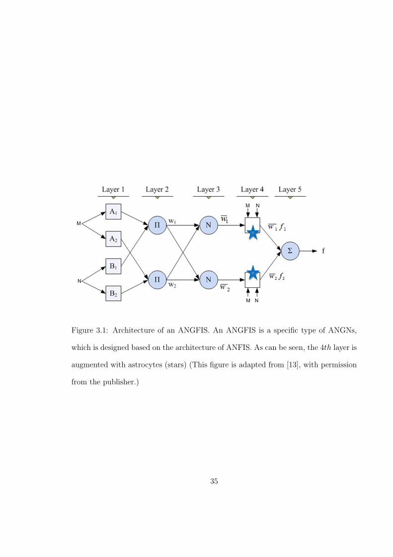
Figure 3.1: Architecture of an ANGFIS. An ANGFIS is a specific type of ANGNs,
which is designed based on the architecture of ANFIS. As can be seen, the 4th layer is
augmented with astrocytes (stars) (This figure is adapted from [13], with permission
from the publisher.)
35

2.4.2, and updates the parameters at the end of each cycle2.
2. The second phase is the algorithm for astrocytes’ learning, and is independent
from the first phase. Astrocytes receive outputs of their corresponding nodes,
and based on the activity of the nodes, independently increase or decrease the
parameters by some pre-defined percentages. Section 2.5 provides a detailed
explanation of the algorithm of each astrocyte.
3.2 Performance
In this section, we investigate the performance of ANGFIS on two problems; and
study how isolated astrocytes in ANGFIS can reduce overall output errors. More
precisely, for testing the performance of ANGFIS, we answer the following question:
Are there parameter values for astrocytes of ANGFIS
that increase the performance of ANGFIS in comparison
to ANFIS?
The implementation described here3 aimed to test the performance of the proposed
ANGFIS and to compare it with ANFIS 4. ANFIS use a back propagation algorithm
for training as explained in Section 2.4.2. The architecture features, such as number of
2A cycle is defined as presenting all training data set to the system.3The implemented codes are available at the supplementary materials of this thesis.4The performance of ANFIS was already evaluated by Jang in 1993 [21]; we will use the same
programming codes to do our implementations.
36
rules, should be decided by an expert; however, in this thesis, we have used the same
number of rules, empirically5 determined by Jang for studying the same problems6
[21]. The training and testing of ANGFIS were implemented on a system with a 3
GHz processor and 3 GB of RAM using the Ubuntu operating system, C language
source code and the GNU compiler; ANGFIS were implemented by modifying the
previous available codes of ANFIS used in [21].
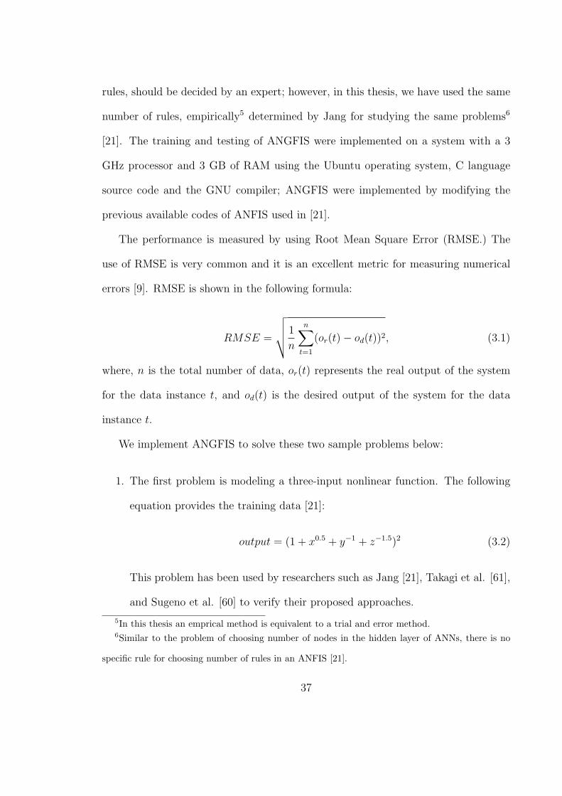
The performance is measured by using Root Mean Square Error (RMSE.) The
use of RMSE is very common and it is an excellent metric for measuring numerical
errors [9]. RMSE is shown in the following formula:
RMSE =
√√√√ 1
n
n∑t=1
(or(t)− od(t))2, (3.1)
where, n is the total number of data, or(t) represents the real output of the system
for the data instance t, and od(t) is the desired output of the system for the data
instance t.
We implement ANGFIS to solve these two sample problems below:
1. The first problem is modeling a three-input nonlinear function. The following
equation provides the training data [21]:
output = (1 + x0.5 + y−1 + z−1.5)2 (3.2)
This problem has been used by researchers such as Jang [21], Takagi et al. [61],
and Sugeno et al. [60] to verify their proposed approaches.
5In this thesis an emprical method is equivalent to a trial and error method.6Similar to the problem of choosing number of nodes in the hidden layer of ANNs, there is no
specific rule for choosing number of rules in an ANFIS [21].
37

2. The second problem aims to identify nonlinear components in a control sys-
tem. The nonlinear F (.) function in the following equations is implemented by
ANGFIS where parameters are updated in each time index [21].
y(k + 1) = 0.3y(k) + 0.6y(k − 1) + F (u(k))), (3.3)
where k represents the time index in the control system, y(k) is output, u(k) is
input. This problem has been used by different researchers, such as Jang [21] ,
and Narendra et al. [37] to verify their proposed approaches.
The ANGFIS designed for the first problem has the general five-layer architecture
of ANFIS (see Figure 3.1). The first (input) layer of ANGFIS has three nodes, each
of which receives one input of the problem instance. The second (membership) layer
has 6 membership functions; the number of nodes in this layer has been empirically
determined by Jang [21] for solving a similar problem by ANFIS. Both of Layers
3 and 4 contain 8 nodes, where each node represents a rule; similarly, the number
of rules has been adapted from [21]. Finally, the fifth layer integrates the output
into one number, and provide us with the final output. For training and testing
ANGFIS, we have used 216 training samples uniformly selected from the input range
[1, 6] × [1, 6] × [1, 6] and 125 testing data in the range of [1.5, 5.5] × [1.5, 5.5]. These
data also were used by Jang for investigating the performance of ANFIS [21]. Each
node in the 4th layer is associated with one astrocyte and the astrocyte parameters
were determined empirically (see Table 3.1.) Detailed information about the astrocyte
parameters is available in Section 2.5.
38
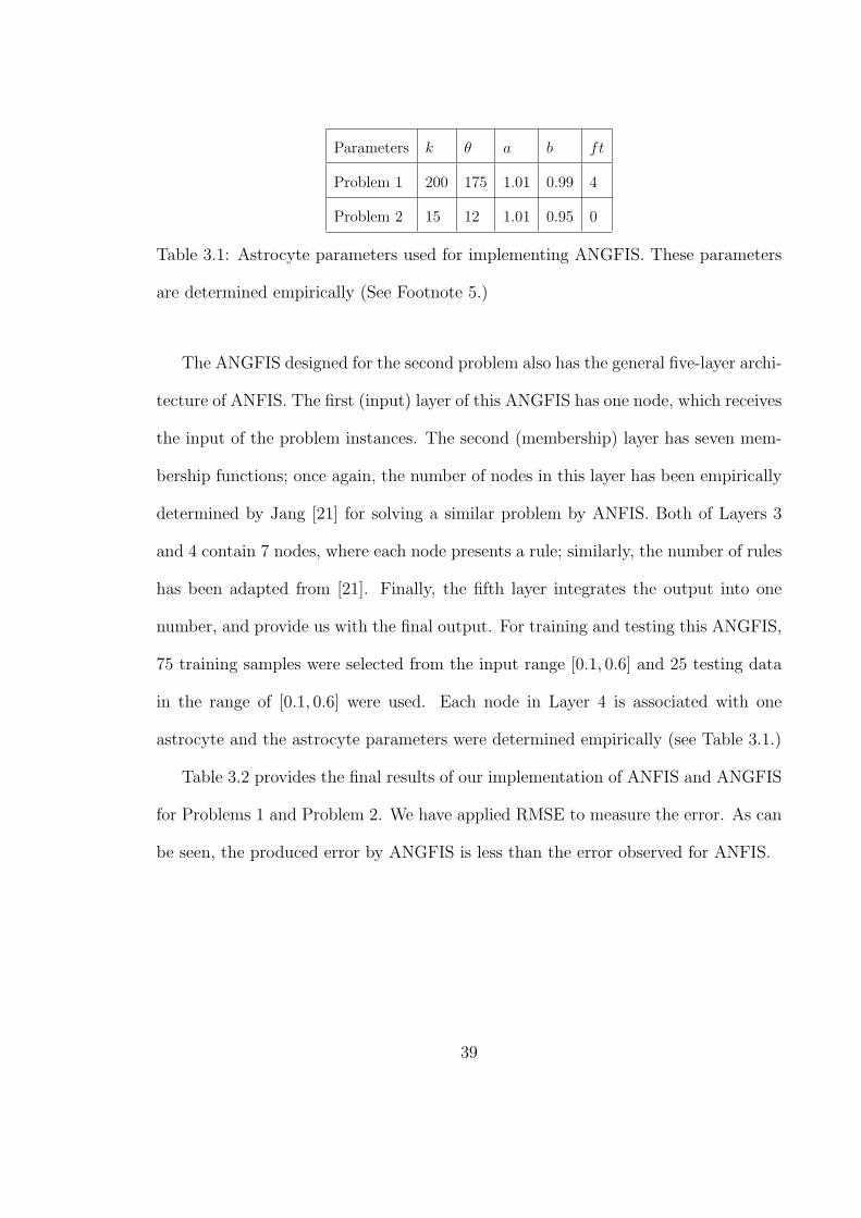
Parameters k θ a b ft
Problem 1 200 175 1.01 0.99 4
Problem 2 15 12 1.01 0.95 0
Table 3.1: Astrocyte parameters used for implementing ANGFIS. These parameters
are determined empirically (See Footnote 5.)
The ANGFIS designed for the second problem also has the general five-layer archi-
tecture of ANFIS. The first (input) layer of this ANGFIS has one node, which receives
the input of the problem instances. The second (membership) layer has seven mem-
bership functions; once again, the number of nodes in this layer has been empirically
determined by Jang [21] for solving a similar problem by ANFIS. Both of Layers 3
and 4 contain 7 nodes, where each node presents a rule; similarly, the number of rules
has been adapted from [21]. Finally, the fifth layer integrates the output into one
number, and provide us with the final output. For training and testing this ANGFIS,
75 training samples were selected from the input range [0.1, 0.6] and 25 testing data
in the range of [0.1, 0.6] were used. Each node in Layer 4 is associated with one
astrocyte and the astrocyte parameters were determined empirically (see Table 3.1.)
Table 3.2 provides the final results of our implementation of ANFIS and ANGFIS
for Problems 1 and Problem 2. We have applied RMSE to measure the error. As can
be seen, the produced error by ANGFIS is less than the error observed for ANFIS.
39

Problem 1 Problem 2
ANFIS (Training Data set) 0.605402 0.168400
ANGFIS (Training Data set) 0.605370 0.057043
ANFIS (Testing Data set) 0.831868 0.258672
ANGFIS (Testing Data set) 0.823220 0.128272
Table 3.2: The RMSE error for ANGFIS and ANFIS.
3.3 Discussion
As is shown in Tables 3.2 and 3.1, by choosing appropriate parameters, the perfor-
mance of ANGFIS can be higher than the performance of ANFIS. The architecture,
activation functions, training algorithm, and also the problems and training and test-
ing data-sets are similar in both implemented ANFIS and ANGFIS; the only difference
is the inclusion of astrocytes in ANGFIS. It means, this difference solely is the result
of inclusion of astrocytes and it can be interpreted as the contribution to performance
made by astrocytes.
Porto in 2011 showed that the inclusion of astrocytes in a feed-forward neural
network (ANGNs) can improve the performance of the network [52] (see Section
2.5). Here we show that the inclusion of astrocytes in a different architecture of
neural networks, ANFIS, can also reduce the error and enhance the performance.
The higher performance achieved by the inclusion of astrocytes can be explained in
two ways. Firstly, inclusion of astrocytes and modeling tripartite synapses provides
us with a more accurate model of the human brain, which is known to be a powerful
information processing system. Secondly, previous research shown that in general,
40

noise and chaotic behavior can help algorithms to escape local minima [58, 67], and
in particular in neural networks it is known that injecting noise during training can
increase the overall performance of the network [35, 2, 75, 29]; here, astrocytes can
be considered as a source of noise in the ANNs that improves performance 7.
For the purpose of further improving the performance of ANGFIS, different mod-
ifications in the architecture and algorithms of astrocytes can be applied. Some
preliminary implementations’ results not reported here suggest that if we modify the
astrocyte’s algorithm in a way that increases the output of neurons rather than mod-
ifying the parameters, the overall RMSE error will also be decreased. Hence, having
astrocytes in all layers rather than only the fourth may increase the performance of
the network. More detailed information on these modifications is given in Chapter 5.
7Researchers such as An [2] and Brown et al.[7] have shown that in their studied networks adding
noise into an artificial neural network will increase the performance. Glia astrocytes by increasing
and decreasing the weights outside the training algorithm of ANNs might be considered as a source
of noise propagation.
41

Chapter 4
Artificial Astrocytes Networks
(AANs)
Artificial Neural Networks (ANNs) (see Section 2.3) are defined as brain-inspired sys-
tems that have the ability to process information and complete tasks in different areas
such as classification, prediction and evaluation. A more recent model of ANNs called
Artificial Neuron-glia Networks (ANGNs) (see Section 2.5) benefit from biologically-
inspired elements, artificial astrocytes. ANGNs model astrocytes as single isolated
elements; however, recent physiological findings summarized in Section 2.2 claim that
activation of one astrocyte propagates to other astrocytes through gap junctions.
Inspired by this new finding, we designed a novel neural network architecture that
benefits from a network of artificial astrocytes on top of a neuron-glia network, rather
than using isolated astrocytes. The remainder of this chapter introduces and evalu-
ates artificial astrocyte networks (AANs). First, in Section 4.1, the architecture of
and the learning algorithm for AANs are introduced; then in Section 4.2, we describe
42

an implementation of an AAN and discuss the results obtained by testing this imple-
mentation on two classification problems. Finally, Section 4.3 presents a discussion
on the AAN performance.
4.1 Architecture and Learning Algorithm
In this section, we present the proposed model of AANs. The first subsection in-
troduces the architecture of AANs, and the second subsection describes the learning
algorithm for AANs.
4.1.1 Architecture
The structure of the artificial astrocyte networks is founded on artifical neuron-glia
networks; each neuron is associated with one astrocyte and the appropriate activity of
the corresponding neuron turns the astrocyte on or off. This structure as presented
in Section 2.2 mimics the release of neurotransmitters by astrocytes in the brain’s
tripartite synapses [50, 4, 52]. In this chapter, in addition to the components of
artificial neuron-glia networks, there are connections between astrocytes that comprise
the astrocyte networks. An active astrocyte results in the activation of all other
astrocytes in the same network. This behavior is inspired by the propagation of
calcium wave through astrocyte’s gap junctions in the brain [49] as presented in
Section 2.2.
43

Figure 4.1: ANGN and AAN. The left image depicts a neuron-glia network (astrocytes
are shown with stars), and the image on the right is a neuron-glia network with an
artificial astrocyte network. The solid lines in the latter image shows one possible
astrocyte network (These figures are adapted from Figure 3 in [52], with permission
from the publisher).
As explained in Section 2.2, the exact nature of the connections between biological
astrocytes is not yet clear. The model we suggest for astrocyte networks is based on
connecting random astrocytes. A set which is composed of n randomly chosen astro-
cytes will be determined. Then, each pair of astrocytes in the set will be connected
by an edge. The result will be a complete astrocyte network (i.e., there is an edge
between each pair of nodes). Having a complete network is inspired by the work of
Pereira and Furlan [49]. Each astrocyte network may contain two to n astrocytes1,
1In each portion of the brain, generally more than one astrocyte network is connected to neurons,
44
where the maximum value for n is the total number of neurons in all layers. The
efficient number of astrocytes participating in an AAN can be determined empirically
(i.e. by trial and error method). Figure 4.1 presents an ANGN and a possible struc-
ture for its corresponding AAN; note that in this figure, the astrocyte network is not
a complete network.
4.1.2 Learning Algorithm
Artificial astrocyte networks use ANGN algorithms (see Section 2.5) plus an extra
algorithm that represents the connections between astrocytes. This extra algorithm,
which implements the signal receiving and sending processes is described in the follow-
ing paragraphs. Each astrocyte in an AAN runs the same algorithm. This algorithm
can be divided into two phases: the first phase determines the state of the astrocyte
(active or inactive), and in the second phase, the weights are updated and signals are
sent to connected astrocytes. The following paragraphs provide more information on
these two phases.
In the first phase, we initially check the input signals to an astrocyte. If the
astrocyte receives an activation signal from a connected astrocyte, then immediately
it will become active and act exactly similar to an active isolated astrocyte2 (a positive
signal will activate the astrocyte positively3 and a negative signal will activate an
astrocyte negatively). If no activation signal is received, then the astrocyte will run
but for simplicity of the artificial networks, in this thesis, we assume that only one astrocyte network
can be implemented on top of an ANN.2This signal receiving process is part of the previously mentioned “extra algorithm”.3From the Physiological perspective, positive and negative activation corresponds to increase and
decrease of synaptic strength respectively.
45
an isolated astrocyte’s algorithm, and check the activity of its corresponding neuron.
All functions and parameters used here are the same as those used in the ANGN
algorithms described in Section 2.5. Lastly, if the activation conditions of an astrocyte
are satisfied (either by receiving an activation signal or by the result of running the
algorithm of isolated astrocyte), the astrocyte will become activated and the second
phase will be started.
The second phase initially updates the weights of active astrocytes by some pre-
defined percentages (the details of this updating process are available in Section 2.5).
Furthermore, in AANs, the active astrocytes send an activation signal to all the
connected astrocytes4(a positive signal if it is positively activated and a negative signal
if it is negatively activated). Figure 4.2 depicts a flowchart of the AAN algorithm for
positively active astrocytes.
4.2 Performance
In this section, we investigate the performance of artificial astrocyte networks on two
classification problems, and study how isolated and networks of artificial astrocytes
can affect the accuracy of classification. For testing the performance of AAN, we
answer the following question:
Are there possible patterns of connections between as-
trocytes of a neuron-glia network that produce more ac-
curate classification results?
4This signal sending process is part of the previously mentioned “extra algorithm”.
46

Figure 4.2: A flowchart of the AAN algorithm. This algorithm is executed by ev-
ery single astrocyte. For simplicity, computations involving -θ, which represents the
negatively active astrocytes, are omitted from the algorithm above.
47

We implement AAN to solve two classification problems5. The first problem is
classifying breast cancer cells into healthy and unhealthy cells6 and the second one
is a classification of ionosphere data into good and bad 7; both problems are binary
classification tasks, which means there are two possibilities for the output and the
input will be categorized either into group one or group two. The breast cancer and
the ionosphere data sets used in this work were part of the UCI data sets [34], which
are based on real world data and repeatedly have been used in the machine learning
literature [71, 69, 70, 74, 24]. As stated eariler, the breast cancer data set categorized
instances into either “healthy” and “unhealthy”. The instances are described by
nine attributes, some of which are linear and others are nominal. The available
286 breast cancer instances in the data set were organized into 143 training and
143 testing instances. The ionosphere data set consisted of 351 instances, with each
instance having 34 attribute classified as either “good” or “bad”. The 351 instances
of ionosphere data set were divided into 175 training and 176 testing instances. The
5The implemented codes are available at the supplementary materials of this thesis.6Originally, this breast cancer domain was obtained from the University Medical Centre, Institute
of Oncology, Ljubljana, Yugoslavia. Thanks go to M. Zwitter and M. Soklic for providing the data.7Based on the information provided in [34] “This data was collected by a system in Goose
Bay, Labrador. This system consists of a phased array of 16 high-frequency antennas with a total
transmitted power on the order of 6.4 kilowatts ... The targets were free electrons in the ionosphere.
“Good” radar returns are those showing evidence of some type of structure in the ionosphere.
“Bad” returns are those that do not; their signals pass through the ionosphere. Received signals
were processed using an auto-correlation function whose arguments are the time of a pulse and the
pulse number. There were 17 pulse numbers for the Goose Bay system. Instances in this database
are described by 2 attributes per pulse number, corresponding to the complex values returned by
the function resulting from the complex electromagnetic signal.”
48

training and testing of the networks were implemented on a system with a 1.30 GHz
processor and 2 GB of RAM using the Windows 8 operating system, Java language
source code and the Eclipse compiler.
These experiments aimed to test the performance of the proposed artificial as-
trocyte networks and to compare them with a typical ANN and ANGN. The typical
ANN is designed as a multi-layer back propagation network which is composed of
three layers. For the breast cancer problem, the input layer consists of nine neurons,
each of which receives one feature of the cells recognized as the input. The output
layer consists of two neurons, which represents healthy and unhealthy cells. The hid-
den layer consists of eight neurons. The number of neurons in the hidden layer was
determined empirically by adjusting the number of neurons in the hidden layer from
1 to 14. For the ionosphere problem, the input layer consisted of 34 neurons, such
that each input neuron corresponds to one input attribute and the output layer had
two neurons, representing “good” and “bad”. The number of neurons in the hidden
layer was also empirically determined to be 18.
The neuron-glia network was implemented on top of the ANN, as explained in
Section 4.1.1 , by including the following astrocyte parameters: k, θ, a,b and ft ∈ R.
The values of these parameters were experimentally determined. Table 4.1 gives the
final parameter values chosen for the training and testing of the networks.
The network of interest in this research, the artificial astrocyte network, was
implemented by employing the same parameters of the ANGN (see Table 4.1). The
astrocyte networks were defined based on the random selection of the astrocytes as
explained in Section 4.1. The astrocyte network for breast cancer data set was tested
by involving three random astrocytes, and for ionosphere data with 5 astrocytes; the
49

Parameters
Neurons
in first
Layer
Neurons
in 2nd
Layer
Neurons
in 3rd
Layer
α k θ a b ft
Breast cancer 9 8 2 0.1 100 40 1.25 0.75 0.75
Ionosphere 34 18 2 0.1 90 27 1.25 0.75 0.6
Table 4.1: Parameters used in implementing ANGN and AAN . The first four columns
define the ANNs. The rest present the parameters related to astrocytes.
Network
Test
Accuracy
(Breast
Cancer)
Test
Accuracy
(Ionosphere)
ANN 0.87 0.80
ANGN 0.91 0.86
AAN 0.93 0.88
Table 4.2: The accuracy of classification on test data for ANN, ANGN and AAN.
accuracy of classification in these experiments on testing data is reported in Table
4.2.
4.3 Discussion
Table 4.2 shows a comparison between typical neural networks, neuron-glia networks
and artificial astrocyte networks. It can be seen that the inclusion of the single as-
50
trocytes (ANGNs) improves the performance of the typical neural network (as also
discussed in [52]) and the performance of ANGNs can further be enhanced by con-
necting astrocytes and forming astrocyte networks. It should be noted that the
common parameters have the same value in all models. Therefore, the variations of
the accuracy between ANN and ANGN is solely for the inclusion of single astrocyte
elements and between ANGN and AANs is for the connections established between
some astrocytes.
In an Artificial Astrocyte Network, providing a complete analysis of the sensitiv-
ity of the error of the network relative to each of the parameters and combination
of parameters requires intensive research in the field of parameter sensitivity. The
complexity of these analysis is due to the relation between the five parameters of
astrocytes to each other, and also the relation of these parameters to the connections
between astrocytes. The possibility of using real values for three of the astrocyte
parameters also increases the complexity of this problem.
A preliminary analysis has shown that there is no linear relation between these
parameters and the error of the network. In the Breast Cancer problem, we set the
value of all parameters except one to a constant values and then varied the value of the
selected parameter. When we did this for parameter a we observed that decreasing
the value of a does not significantly affect the results; however, increasing the value
of a decreases the performance and reduce the accuracy from 0.96 to around 0.5. On
the other hand, the parameter b does not follow the same behavior: increasing b first
increases the accuracy, then decrease it and finally again increase it. For the parame-
ters k and ft, the same behavior is observed. But for the parameter θ the behavior is
different again: from the value zero to a specific point, there is no significant change
51

in the performance, and after that specific point the performance increases in a non
linear manner. This demonstrates that astrocyte parameters have complex individual
behaviors and are thus likely to have even more complex behaviours when they are
co-varied. In Future research we will investigate in much greater depth the relation
of these parameters and their effects on the error of the network.
The higher computing power achieved by the inclusion of the artificial astrocyte
networks can be explained in two ways. Firstly, there is some similarity between
AANs and liquid state machines [38], and recurrent neural networks [11], which re-
sults in the reception of time-varying inputs from external astrocyte sources, as well
as neurons. In the AAN algorithm, astrocytes are randomly connected to each other.
The recurrent nature of the connections turns the time varying input into a spatio-
temporal pattern of activation in the network nodes that enables the network to
compute a large variety of non-linear functions on the input. In other words, the
astrocytes serve as a memory that records information about the past k cycles and
allow the use of this information to shape the network in a way that reduces error.
Secondly, from a physiological point of view, astrocyte networks give a simple inter-
pretation of data integration in the brain [49]. Therefore, having an AAN on top
of typical neural networks add the benefit of data integration; this gives us a more
realistic model of the human brain that is able to provide a more detailed analysis
and yields a more powerful artificial neural network.
To further improve the performance of AANs, we can apply different modification
to AANs and determine if any of these modifications will improve the results. Two
possible modifications are
52

• First, we can modify the algorithm of single isolated astrocytes by assigning each
astrocytes an activation function, or we can directly increase or decrease the
output of the associated neurons rather than modifying the associated weights.
• Second, we can modify the network of astrocytes by having some separate
structurally-different astrocyte networks on top of an ANN, or corresponding
more than one astrocyte (neuron) to a neuron (astrocyte).
53
Chapter 5
Summary and Future Work
In this chapter, we first provide a summary of the research done in this thesis and
then discuss the possible directions for future work.
5.1 Summary
The learning procedures in the human brain inspired researchers to develop tools
such as artificial neural networks that have the ability to learn. Artificial neural
networks (ANN) attempt to imitate the structure of biological neural networks. In
Chapter 2 first, we provided some information on recent research in biology that
indicates astrocytes in addition to neurons are responsible for processing information
in the human brain. Then in Section 2.5, we explained how this concept is found
its way into artificial intelligence and is modeled in feed-forward multi-layer artificial
neural networks called Artificial Neuron-glia Networks (ANGN). In Chapters 3 and
4, in continuation of this research, we proposed two models of artificial neuron-glia
networks. In Chapter 3, we added artificial astrocytes into a different architecture
54

of neural networks, adaptive neuro fuzzy inference systems (ANFIS), and evaluated
the performance of such systems with and without the inclusion of astrocytes. Our
results show that including astrocytes with some specific parameter values will result
in some improvements in the performance of the system. In Chapter 4, we proposed
the concept of artificial astrocyte networks, and showed that connecting astrocytes to
each other and making a network of astrocytes on top of a feed-forward multi-layer
neural network can result in more accurate classification results and thus enhance the
performance of such networks.
Taken together, our set of results suggested that for some specific parameter values
representing networks and astrocytes, we can achieve more accurate results rather
than typical neural networks. This provides us with some insight on how an artificial
astrocyte might be an appropriate element for increasing the performance of ANNs;
however our specific results for specific problems do not yet answer the question of
whether our proposed models will be successful in general or not. The next section
sketches some directions for future work that will help us to answer this question.
5.2 Future Work
The research on ANGFIS presented in this thesis can be continued in five ways.
1. We can implement ANGFIS for solving a greater variety of real-world prob-
lems than those examined in this thesis, such as EEG signal processing, and
investigate how each single and combination of astrocyte parameters affect the
results of each problem. This can then be used to find general rules for choosing
astrocytes parameter values.
55

2. We can have a comparison between noise, chaotic behavior and astrocytes to
study if astrocytes obey the current models on noise propagation and chaotic
behaviors in neural networks and thus answer the question if we can use current
models of noise injection in the networks to describe the behavior of astrocytes
in artificial and biological neural networks.
3. We can analyze the training of astrocyte-enhanced fuzzy networks from the clas-
sical and parameterized computational complexity perspective; these analyses
will hopefully help us to design more efficient models of astrocytes.
4. We can implement astrocytes on other ANN architectures, such as learning vec-
tor quantization [11, 12], bidirectional associative memory [11, 12], and adaptive
resonance theory [11, 12] to study how the inclusion of astrocytes will affect the
results.
5. We can include astrocytes in other layers of ANFIS rather than the fourth
layer, and design more neurally realistic parameters and functions for modeling
astrocytes, and study the resulting changes in the performance of networks.
Possible future work on AANs can be divided into four main directions.
1. We can focus on designing more accurate models for describing artificial as-
trocytes and astrocyte networks. Since 2004, when artificial astrocytes were
introduced until now, new physiological studies revealed other aspects of the
functionality and structure of astrocytes and their networks [14, 17, 49]; a sim-
plified version of these aspects, specifically astrocyte networks with the ability
to learn can be added to current astrocyte models. We can also provide more
56

realistic models of astrocytes in their distribution in the network such as con-
necting one astrocyte to several nodes, or having random number of astrocytes
on random nodes in the network,
2. We can address theoretical issues regarding the computational complexity of
training astrocyte-enhanced networks. Analyzing these networks from the com-
putational complexity perspective in general and parametrized complexity in
particular, will help us to recognize the aspects of these networks that allow
restricted networks that operate more quickly.
3. We can implement AANs on different neural network architectures and evaluate
their performance with and without the added astrocyte networks.
4. We can evaluate other types of astrocyte networks. In this work, we only
test the performance of one random astrocyte network. It may be of use to
evaluate the performance by considering all types of astrocyte networks, which
are represented in the form of trees, bi-partite graphs or other types of graphs.
Delays in transmitting data on astrocyte connections could also be considered
in these networks.
57

Bibliography
[1] A. Alvarellos-Gonzalez, A. Pazos, and A. B. Porto-Pazos. Computational models
of neuron-astrocyte interactions lead to improved efficacy in the performance of
neural networks. Computational and Mathematical Methods in Medicine, 2012,
2012.
[2] G. An. The effects of adding noise during backpropagation training on a gener-
alization performance. Neural Computation, 8(3):643–674, 1996.
[3] A. Araque, G. Carmignoto, and P. G. Haydon. Dynamic signaling between
astrocytes and neurons. Annual Review of Physiology, 63(1):795–813, 2001.
[4] A. Araque, V. Parpura, R. P. Sanzgiri, and P. G. Haydon. Tripartite synapses:
glia, the unacknowledged partner. Trends in Neurosciences, 22(5):208–215, 1999.
[5] R. Bharath and J. Drosen. Neural Network Computing. Windcrest/McGraw-Hill,
1994.
[6] C. Bonansco, A. Couve, G. Perea, C. A. Ferradas, M. Roncagliolo, and M. Fuen-
zalida. Glutamate released spontaneously from astrocytes sets the threshold for
synaptic plasticity. European Journal of Neuroscience, 33(8):1483–1492, 2011.
58

[7] W. M. Brown, T. D. Gedeon, and D. I. Groves. Use of noise to augment training
data: a neural network method of mineral–potential mapping in regions of limited
known deposit examples. Natural Resources Research, 12(2):141–152, 2003.
[8] E. P. Cook, J. A. Guest, Y. Liang, N. Y. Masse, and C. M. Colbert. Dendrite-to-
soma input/output function of continuous time-varying signals in hippocampal
ca1 pyramidal neurons. Journal of Neurophysiology, 98(5):2943–2955, 2007.
[9] P. E. Dennison, K. Q. Halligan, and D. A. Roberts. A comparison of error metrics
and constraints for multiple endmember spectral mixture analysis and spectral
angle mapper. Remote Sensing of Environment, 93(3):359–367, 2004.
[10] M. O. Efe and O. Kaynak. A comparative study of neural network structures in
identification of nonlinear systems. Mechatronics, 9(3):287–300, 1999.
[11] L. V. Fausett. Fundamentals of Neural Networks. Prentice-Hall, 1994.
[12] J. A. Freeman and D. M. Skapura. Neural Networks: Algorithms, Applications,
and Programming Techniques. Addison-Wesley Publishing Company, 1991.
[13] T. M. Geronimo, C. E. Cruz, E. C. Bianchi, F. de Souza Campos, and P. R.
Aguiar. MLP and ANFIS Applied to the Prediction of Hole Diameters in the
Drilling Process. INTECH Open Access Publisher, 2013.
[14] C. Giaume, A. Koulakoff, L. Roux, D. Holcman, and N. Rouach. Astroglial net-
works: a step further in neuroglial and gliovascular interactions. Nature Reviews
Neuroscience, 11(2):87–99, 2010.
59
[15] I. Guler and E. D. Ubeyli. Adaptive neuro-fuzzy inference system for classifica-
tion of EEG signals using wavelet coefficients. Journal of Neuroscience Methods,
148(2):113–121, 2005.
[16] G. I. Hatton and V. Parpura. Glial neuronal signaling, volume 1. Springer, 2004.
[17] P. G. Haydon. Glia: listening and talking to the synapse. Nature Reviews
Neuroscience, 2(3):185–193, 2001.
[18] C. Ikuta, Y. Uwate, and Y. Nishio. Chaos glial network connected to multi-
layer perceptron for solving two-spiral problem. In Proceedings of 2010 IEEE
International Symposium on Circuits and Systems (ISCAS),, pages 1360–1363.
IEEE, 2010.
[19] C. Ikuta, Y. Uwate, and Y. Nishio. Performance and features of multi-layer
perceptron with impulse glial network. In Proceeding of The 2011 International
Joint Conference on Neural Networks (IJCNN), pages 2536–2541. IEEE, 2011.
[20] J.-S. Jang. Self-learning fuzzy controllers based on temporal backpropagation.
IEEE Transactions on Neural Networks, 3(5):714–723, 1992.
[21] J.-S. Jang. ANFIS: adaptive-network-based fuzzy inference system. IEEE Trans-
actions on Systems Man and Cybernetics, 23(3):665–685, 1993.
[22] J.-S. R. Jang et al. Fuzzy modeling using generalized neural networks and kalman
filter algorithm. In Proceedings of the Ninth National Conference on Artificial
Intelligence, volume 91, pages 762–767, 1991.
60
[23] J.-S. R. Jang, C.-T. Sun, and E. Mizutani. Neuro-fuzzy and soft computing-
a computational approach to learning and machine intelligence [book review].
IEEE Transactions on Automatic Control, 42(10):1482–1484, 1997.
[24] H. Kim and H. Park. Data reduction in support vector machines by a kernelized
ionic interaction model. In SDM, pages 507–511. SIAM, 2004.
[25] E. KONISHI. Modeling quantum mechanical observers via neural-glial networks.
International Journal of Modern Physics B, 26(09):1250060, 2012.
[26] J. Lallouette and H. Berry. Topology drives calcium wave propagation in 3d
astrocyte networks. In Proceedings of the European Conference on Complex Sys-
tems 2012, pages 453–463. Springer, 2013.
[27] H. Landahl, W. S. McCulloch, and W. Pitts. A statistical consequence of the
logical calculus of nervous nets. Bulletin of Mathematical Biology, 5(4):135–137,
1943.
[28] C.-C. J. Lee. Investigation of synaptic plasticity as memory formation mecha-
nism and pathological amyloid fibrillation caused by amyloids aggregation: Mod-
eling work combined with experiments. PhD thesis, Massachusetts Institute of
Technology, 2008.
[29] S. Z. Li. Improving convergence and solution quality of Hopfield-type neural
networks with augmented lagrange multipliers. IEEE Transactions on Neural
Networks, 7(6):1507–1516, 1996.
[30] S.-P. Lo. The application of an ANFIS and grey system method in turning
61

tool-failure detection. The International Journal of Advanced Manufacturing
Technology, 19(8):564–572, 2002.
[31] V. G. Maltarollo, A. B. F. da Silva, and K. M. Honorio. Applications of Artificial
Neural Networks in Chemical Problems. INTECH Open Access Publisher, 2013.
[32] M. Margaliot. Biomimicry and fuzzy modeling: A match made in heaven. Com-
putational Intelligence Magazine, IEEE, 3(3):38–48, 2008.
[33] W. S. McCulloch and W. Pitts. A logical calculus of the ideas immanent in
nervous activity. Bulletin of Mathematical Biophysics, 5(4):115–133, 1943.
[34] P. Murphy and D. Aha. UCI repository of machine learning databases, University
of California, Department of Information and Computer Science, Irvine, CA,
1994.
[35] A. F. Murray and P. J. Edwards. Enhanced MLP performance and fault tolerance
resulting from synaptic weight noise during training. IEEE Transactions on
Neural Networks, 5(5):792–802, 1994.
[36] L. Naderloo, R. Alimardani, M. Omid, F. Sarmadian, P. Javadikia, M. Y. Torabi,
and F. Alimardani. Application of ANFIS to predict crop yield based on different
energy inputs. Measurement, 45(6):1406–1413, 2012.
[37] K. S. Narendra and K. Parthasarathy. Identification and control of dynamical
systems using neural networks. IEEE Transactions on Neural Networks, 1(1):4–
27, 1990.
62
[38] T. Natschlager, W. Maass, and H. Markram. The” liquid computer”: A novel
strategy for real-time computing on time series. Special Issue on Foundations of
Information Processing of TELEMATIK, 8:39–43, 2002.
[39] E. A. Newman. New roles for astrocytes: regulation of synaptic transmission.
Trends in neurosciences, 26(10):536–542, 2003.
[40] C. R. Noback, N. L. Strominger, R. J. Demarest, and D. A. Ruggiero. The
human Nervous System: Structure and Function. Springer, 2005.
[41] U. Pannasch, L. Vargova, J. Reingruber, P. Ezan, D. Holcman, C. Giaume,
E. Sykova, and N. Rouach. Astroglial networks scale synaptic activity and plas-
ticity. Proceedings of the National Academy of Sciences, 108(20):8467–8472, 2011.
[42] L. Pasti, A. Volterra, T. Pozzan, and G. Carmignoto. Intracellular calcium oscil-
lations in astrocytes: a highly plastic, bidirectional form of communication be-
tween neurons and astrocytes in situ. The Journal of Neuroscience, 17(20):7817–
7830, 1997.
[43] D. W. Patterson. Artificial Neural Networks: Theory and Applications. Prentice
Hall PTR, 1998.
[44] G. Perea and A. Araque. Communication between astrocytes and neurons: a
complex language. Journal of Physiology-Paris, 96(3):199–207, 2002.
[45] G. Perea and A. Araque. Properties of synaptically evoked astrocyte calcium
signal reveal synaptic information processing by astrocytes. The Journal of Neu-
roscience, 25(9):2192–2203, 2005.
63
[46] G. Perea and A. Araque. Astrocytes potentiate transmitter release at single
hippocampal synapses. Science, 317(5841):1083–1086, 2007.
[47] G. Perea and A. Araque. Glia modulates synaptic transmission. Brain Research
Reviews, 63(1):93–102, 2010.
[48] G. Perea, M. Navarrete, and A. Araque. Tripartite synapses: astrocytes process
and control synaptic information. Trends in Neurosciences, 32(8):421–431, 2009.
[49] A. Pereira Jr and F. A. Furlan. Astrocytes and human cognition: modeling
information integration and modulation of neuronal activity. Progress in Neuro-
biology, 92(3):405–420, 2010.
[50] T. M. Pirttimaki and H. R. Parri. Astrocyte plasticity implications for synaptic
and neuronal activity. The Neuroscientist, 19(6):604–615, 2013.
[51] A. Porto. Computational models for optimizing the learning and the informa-
tion processing in adaptive systems. PhD thesis, Faculty of Computer Science,
University of A Coruna, 2004.
[52] A. B. Porto-Pazos, N. Veiguela, P. Mesejo, M. Navarrete, A. Alvarellos,
O. Ibanez, A. Pazos, and A. Araque. Artificial astrocytes improve neural network
performance. PloS One, 6(4), 2011.
[53] J. M. Robertson. The astrocentric hypothesis: proposed role of astrocytes in
consciousness and memory formation. Journal of Physiology-Paris, 96(3):251–
255, 2002.
64
[54] R. Rojas. Neural networks: a systematic introduction. Springer Science & Busi-
ness Media, 1996.
[55] D. A. Rusakov, K. Zheng, and C. Henneberger. Astrocytes as regulators of
synaptic function a quest for the ca2+ master key. the Neuroscientist, 17(5):513–
523, 2011.
[56] Z. Sajedinia. Artificial glia astrocytes; a new element in adaptive neuro fuzzy
systems. Proceedings of the 22th Annual Newfoundland Electrical and Computer
Engineering Conference (NECEC 2013), 2013.
[57] Z. Sajedinia. Artificial astrocyte networks, as components in artificial neural
networks. In Unconventional Computation and Natural Computation, pages 316–
326. Springer, 2014.
[58] B. Selman, H. A. Kautz, and B. Cohen. Noise strategies for improving local
search. In AAAI, volume 94, pages 337–343, 1994.
[59] L. R. Squire. Fundamental Neuroscience. Academic Press, 2013.
[60] M. Sugeno and G. Kang. Structure identification of fuzzy model. Fuzzy Sets and
Systems, 28(1):15–33, 1988.
[61] H. Takagi and I. Hayashi. Nn-driven fuzzy reasoning. International Journal of
Approximate Reasoning, 5(3):191–212, 1991.
[62] T. Takagi and M. Sugeno. Fuzzy identification of systems and its applications
to modeling and control. IEEE Transactions on Systems, Man and Cybernetics,
(1):116–132, 1985.
65
[63] Z. Tan, C. Quek, and P. Y. Cheng. Stock trading with cycles: A financial appli-
cation of ANFIS and reinforcement learning. Expert Systems with Applications,
38(5):4741–4755, 2011.
[64] M. K. Temburni and M. H. Jacob. New functions for glia in the brain. Proceedings
of the National Academy of Sciences, 98(7):3631–3632, 2001.
[65] C. Thome, T. Kelly, A. Yanez, C. Schultz, M. Engelhardt, S. B. Cambridge,
M. Both, A. Draguhn, H. Beck, and A. V. Egorov. Axon-carrying dendrites
convey privileged synaptic input in hippocampal neurons. Neuron, 83(6):1418–
1430, 2014.
[66] G. Trevor. Online resources: Gallant’s Biology Stuff. http:// kvhs. nbed. nb.
ca/ gallant/ biology/biology. html, 2015.
[67] M. van Turnhout and F. Bociort. Chaotic behavior in an algorithm to escape
from poor local minima in lens design. Optics Express, 17(8):6436–6450, 2009.
[68] J. Wade, L. McDaid, J. Harkin, V. Crunelli, and S. Kelso. Self-repair in a bidi-
rectionally coupled astrocyte-neuron (an) system based on retrograde signaling.
Frontiers in Computational Neuroscience.
[69] W. H. Wolberg, W. N. Street, D. M. Heisey, and O. L. Mangasarian. Comput-
erized breast cancer diagnosis and prognosis from fine-needle aspirates. Archives
of Surgery, 130(5):511, 1995.
[70] W. H. Wolberg, W. N. Street, and O. Mangasarian. Machine learning techniques
66

to diagnose breast cancer from image-processed nuclear features of fine needle
aspirates. Cancer Letters, 77(2):163–171, 1994.
[71] W. H. Wolberg, W. N. Street, and O. L. Mangasarian. Image analysis and
machine learning applied to breast cancer diagnosis and prognosis. Analytical
and Quantitative Cytology and Histology, 17(2):77–87, 1995.
[72] L. A. Zadeh. Fuzzy sets. Information and Control, 8(3):338–353, 1965.
[73] L. A. Zadeh. Outline of a new approach to the analysis of complex systems
and decision processes. IEEE Transactions on Systems, Man and Cybernetics,
(1):28–44, 1973.
[74] Z.-H. Zhou and Y. Jiang. Neural ensemble based c4. IEEE Transactions on
Knowledge and Data Engineering, 16:770–773, 2004.
[75] R. M. Zur, Y. Jiang, L. L. Pesce, and K. Drukker. Noise injection for training
artificial neural networks: A comparison with weight decay and early stopping.
Medical Physics, 36(10):4810–4818, 2009.
67