What reflects investor sentiment? Empirical evidence from ...

Giving Content to Investor Sentiment:
The Role of Media in the Stock Market
Paul C.Tetlock∗
ABSTRACT
I quantitatively measure the nature of the media’s interactions with the stock
market using daily content from a popular Wall Street Journal column. I find
that high media pessimism predicts downward pressure on market prices followed
by a reversion to fundamentals, and unusually high or low pessimism predicts high
market trading volume. These results and others are consistent with theoretical
models of noise and liquidity traders. However, the evidence is inconsistent with
theories of media content as a proxy for new information about fundamental asset
values, as a proxy for market volatility, or as a sideshow with no relationship to
asset markets.
∗Tetlock is at the McCombs School of Business, University of Texas at Austin. I am indebted to RobertStambaugh (the editor), an anonymous associate editor and an anonymous referee for their suggestions. Iam grateful to Aydogan Alti, John Campbell, Lorenzo Garlappi, Xavier Gabaix, Matthew Gentzkow, JohnGriffin, Seema Jayachandran, David Laibson, Terry Murray, Alvin Roth, Laura Starks, Jeremy Stein, PhilipTetlock, Sheridan Titman and Roberto Wessels for their comments. I thank Philip Stone for providing theGeneral Inquirer software and Nathan Tefft for his technical expertise. I appreciate Robert O’Brien’s help inproviding information about the Wall Street Journal. I also acknowledge the National Science Foundation,Harvard University and the University of Texas at Austin for their financial support. All mistakes in thisarticle are my own.
1

One of the more fascinating sections of the WSJ is on the inside of the back
page under the standing headline “Abreast of the Market.” There you can read
each day what the market did yesterday, whether it went up, down or sideways as
measured by indexes like the Dow Jones Industrial Average . . . . In that column,
you can also read selected post-mortems from brokerage houses, stock analysts
and other professional track watchers explaining why the market yesterday did
whatever it did, sometimes with predictive nuggets about what it will do today
or tomorrow. This is where the fascination lies. For no matter what the market
did–up, down or sideways–somebody will have a ready explanation. ... -
Vermont Royster (January 15, 1986)
Casual observation suggests the content of financial news about the stock market could be
linked to investor psychology and sociology. However, it is unclear whether the financial
news media induces, amplifies or simply reflects investors’ interpretations of stock market
performance. This paper attempts to characterize the relationship between the content of
media reports and daily stock market activity, focusing on the immediate influence of the
Wall Street Journal ’s (WSJ ’s) “Abreast of the Market” column on U.S. stock market returns.
To my knowledge, this paper is the first to find evidence that news media content can
predict movements in broad indicators of stock market activity. Using principal components
analysis, I construct a simple measure of media pessimism from the content of the WSJ
column. Then I estimate the intertemporal links between this measure of media pessimism
and the stock market in basic vector auto-regressions (VARs). First and foremost, I find
that high levels of media pessimism robustly predict downward pressure on market prices,
followed by a reversion to fundamentals. Second, unusually high or low values of media
pessimism forecast high market trading volume. Third, low market returns lead to high
media pessimism. These findings suggest that measures of media content serve as a proxy
2

for investor sentiment or non-informational trading. By contrast, statistical tests reject the
hypothesis that media content contains new information about fundamental asset values and
the hypothesis that media content is a sideshow with no relation to asset markets.
I use the General Inquirer (GI), a well-known quantitative content analysis program,
to analyze daily variation in the WSJ “Abreast of the Market” column over the 16-year
period 1984 to 1999 inclusive. This column is a natural choice for a data source that reflects
and influences investor sentiment for three reasons. First, the WSJ has by far the largest
circulation–over 2 million readers–of any daily financial publication in the U.S. and Dow
Jones Newswires, the preferred medium for electronicWSJ distribution, reaches over 325,000
finance and investment professionals.1 Second, theWSJ and Dow Jones Newswires, founded
in 1889 and 1897 respectively, are extremely well-established and have strong reputations
with investors. Third, electronic texts of the WSJ “Abreast of the Market” column are
accessible over a longer time horizon than texts of any other column about the stock market.2
For each day in my sample, I gather newspaper data by counting the words in all 77 prede-
termined GI categories from the Harvard psychosocial dictionary. To mitigate measurement
error and enhance construct validity, I perform a principal components factor analysis of
these categories. This process collapses the 77 categories into a single media factor that
captures the maximum variance in the GI categories. Because this single media factor is
strongly related to pessimistic words in the newspaper column, I refer to it as a pessimism
factor hereafter.
In standard return predictability regressions, changes in this pessimism factor predict sta-
tistically significant and economically meaningful changes in the distribution of daily U.S.
stock returns and volume. I confirm the robustness of this relationship by looking at the
sensitivity of the results to the timing of information and to the use of different measures
of pessimism. The results remain the same when I allow for a significant time gap between
the release of media pessimism and the event return window. I also replicate the results
3

using alternative measures of media pessimism based on the original GI categories. Using
the GI category for either Negative words or Weak words (the two GI categories most highly
correlated with pessimism), I find similar relationships between the media and the market.
This approach to modeling behavioral phenomena yields factors and corresponding regres-
sion coefficients that can be readily interpreted in terms of well-established psychological
variables.
Section I provides some context and motivation for studying the impact of the media
on the stock market. Section II describes the factor analysis of the content of the daily
“Abreast of the Market” column in the Wall Street Journal. Section III reports myriad
tests of whether the pessimism media factor correlates with future stock market activity. In
Section IV, I interpret the pessimism factor in terms of investor sentiment and show that
the risk premium explanation does not explain the results. I conclude in Section V with a
brief discussion of the results and suggestions for future research on the influence of media in
asset markets. Finally, because this study relies heavily on a technique unfamiliar to many
economists, the Appendix introduces the method of quantitative content analysis as it is
employed in this study–for more detailed information, see Riffe, Lacy, and Fico (1998).
I. Theory and Background
Since John Maynard Keynes coined the term animal spirits 70 years ago, economists have
devoted substantial attention to trying to understand the determinants of wild movements
in stock market prices that are seemingly unjustified by fundamentals (see Keynes (1936)).
Cutler, Poterba, and Summers (1989) is one of the first empirical studies to question the
link between news coverage and stock prices. Surprisingly, the authors find that important
qualitative news stories do not seem to help explain large market returns unaccompanied by
quantitative macroeconomic events.
4

Two recent studies identify interesting relationships between trading volume and mea-
sures of communication activity. Antweiler and Frank (2004) study messages in Internet
chat rooms focused on stocks, characterizing the content of the messages as “buy,” “sell” or
“hold” recommendations. Although they do not find a statistically or economically signifi-
cant effect of “bullish” messages on returns, Antweiler and Frank (2004) do find evidence of
relationships between message activity and trading volume and message activity and return
volatility. Similarly, Coval and Shumway (2001) establish that the ambient noise level in a
futures pit is linked to volume, volatility and depth–but not returns.
Most theoretical models of the effect of investor sentiment on stock market pricing make
two important assumptions–see, for example, DeLong et al. (1990a). First, these models
posit two types of traders: noise traders who hold random beliefs about future dividends
and rational arbitrageurs who hold Bayesian beliefs. In this paper, I will refer to the level
of noise traders’ beliefs relative to Bayesian beliefs as investor sentiment. For example,
when noise traders have expectations of future dividends that are below the expectations of
rational arbitrageurs, I will call their beliefs pessimistic. Further, I will assume that these
misperceptions of dividends are stationary, implying that beliefs do not stray arbitrarily far
from Bayesian expectations over time.
Second, both types of traders have downward-sloping demands for risky assets because
they are risk-averse, capital-constrained, or otherwise impaired from freely buying and selling
risky assets. These assumptions lead to an equilibrium in which noise traders’ random
beliefs about future dividends influence prices. When noise traders experience a negative
belief shock, they sell stocks to arbitrageurs, increasing volume and temporarily depressing
returns. On average, returns rebound next period when there is a new belief shock because
these shocks are stationary. Thus, models of investor sentiment such as DeLong et al.(1990a)
predict low sentiment will produce downward price pressure and unusually high or low values
of sentiment will generate high volume.
5

More generally, models of trade for any non-informational reason, such as liquidity needs
or sudden changes in risk aversion, make these same predictions. For example, Campbell,
Grossman, and Wang (1993) model how changes in the level of risk aversion for a large
subset of investors can affect short-term returns. The only way to distinguish noise trader
and liquidity trader theories is to interpret the media pessimism variable as a proxy for
either investor sentiment or risk aversion. Because this debate is more philosophical than
economic, I defer to the reader to draw her own conclusions.
The timing of media pessimism is important in each theory. This paper will test the
specific hypothesis that high media pessimism is associated with low investor sentiment,
resulting in downward pressure on prices. It is unclear whether media pessimism forecasts
investor sentiment or reflects past investor sentiment. If the former hypothesis is correct,
then one would expect high media pessimism to predict low returns at short horizons and a
reversion to fundamentals at longer horizons. If the latter theory is correct, then one would
expect high media pessimism to follow low returns and predict high returns in the future.
The most likely scenario, however, is that both theories have an element of truth. If
media pessimism serves as a proxy for periods of low past and future investor sentiment, one
would expect to find that high pessimism follows periods of low past returns, forecasts low
future returns at short horizons, and predicts high future returns at longer horizons. Insofar
as pessimism reflects past investor sentiment, the high long-horizon returns will exceed the
low short-horizon returns. These predictions concerning returns are summarized in Figure
1.
[Insert Figure 1 around here]
One alternative hypothesis is that the media pessimism measure is a proxy for negative
information about the fundamental values of equities that is not currently incorporated into
prices. If pessimism reflects negative news about past and future cash flows rather than
sentiment, then one would still observe a negative relationship between media pessimism
6

and short-horizon returns. However, the sentiment and information theories make different
predictions about long-horizon returns and volume. Whereas the sentiment theory predicts
short-horizon returns will be reversed in the long run, the information theory predicts they
will persist indefinitely.
Although this discussion focuses on extreme views of the newspaper column as either
pure noise or pure information, it is also possible that the column contains some information
but traders over- or underreact to this information. I will explore these possibilities further
in the empirical tests in Section III.
Another theory of media pessimism is that it is a proxy for negative information about
dividends that is already incorporated into prices. This theory predicts media pessimism
should have no effect on future market activity. Similarly, if one believes that the media
pessimism measure contains no information about past, present, and future dividends, then
one would not expect to observe any impact of pessimism on market activity. Many econo-
mists who have read the “Abreast of the Market” column in theWSJ support some variant
of this theory, believing the column’s goal is to entertain readers.
Trading volume provides another measure of market behavior for assessing theories of
media pessimism. If media pessimism either reflects past or predicts future investor sen-
timent, unusually high or low levels of pessimism should be associated with increases in
trading volume. More precisely, if pessimism has a mean of zero, then the absolute value of
pessimism is high in times when irrational investors trade with rational investors.3 Whereas
the sentiment theory makes a clear prediction about the relationship between volume and
pessimism, the information theory makes no obvious prediction.4 Finally, the stale or no
information theory predicts no effect of media pessimism on trading volume.
7

II. Generating the Pessimism Media Factor
As a completely automated program, the General Inquirer (GI) produces a systematic
and easily replicable analysis of theWSJ column. The GI employs an extremely rudimentary
measurement rule for converting the column into numeric values: it counts the number of
words in each day’s column that fall within various word categories. The word categories are
neither mutually exclusive nor exhaustive–one word may fall into multiple categories and
some words are not categorized at all. To reduce redundancy in categorization, I use only
the most recent versions of categories in the General Inquirer’s Harvard IV-4 psychosocial
dictionary.
To minimize semantic and stylistic noise in the column, I re-center all GI categories so
that their conditional means are equal across different days of the week. This ensures that
I do not select media factors that capture the systematic variation in the WSJ column on
different days of the week. I use day-of-the-week dummy variables in the regressions in the
next section to control for the possibility that market behavior differs across different days
of the week.
I employ a principal components factor analysis to extract the most important semantic
component from the (77x77) variance-covariance matrix of the categories in the Harvard
dictionary. This process is designed to detect complex structure in the WSJ column and to
eliminate the redundant categories in the dictionary. Factor analysis assumes the existence
of an underlying media factor–a linear combination of GI categories that is not directly
observable.5 Variation in this factor over time generates the observed daily correlations
between the various GI categories.
Operationally, factor analysis chooses the vector in the 77-dimensional GI category space
with the greatest variance, where each GI category is given equal weight in the total vari-
ance calculation. I have explored other factor analysis techniques, such as principal factors
8

analysis and maximum-likelihood factor analysis. The qualitative empirical conclusions are
not sensitive to the methodology chosen, and the quantitative conclusions change only min-
imally. For the remainder of this paper, I will present the results using the single factor
identified by principal components analysis that captures the maximum variation in GI cat-
egories. Principal components analysis effectively performs a singular value decomposition
of the correlation matrix of GI categories measured over time. The single factor selected in
this study is the eigenvector in the decomposition with the highest eigenvalue.
Because this singular value decomposition uses only the GI category variables in the cor-
relation matrix, completely disregarding all stock market variables, the resulting media factor
will not necessarily correspond to any traditional measurements of past market performance.
Also, because I did not subjectively eliminate any categories, the factor analysis generates a
media factor that equally considers all sources of variation in theWSJ column, even though
it is likely that some categories are more relevant for measuring investor sentiment.6 Theo-
retical imprecision is the cost of avoiding data mining. To facilitate the interpretation of the
single factor chosen, I will adopt a complementary approach to creating a summary media
variable later in the paper.
The principal components analysis exploits time variation in GI category word counts to
identify the media factor. To avoid data mining and any look-ahead bias in the regressions
that follow, I construct the media factor using only information available to traders. I
estimate the factor loadings in year t − 1 using principal components analysis. Then I use
these loadings, along with the daily word counts in year t, to calculate the values of the
factor throughout year t. Because this procedure does not guarantee any consistency in
factor loadings across years, it is possible that changes in the structure of media content over
time will cause this procedure to generate a meaningless factor. For example, if the column
writer focuses on different issues in different years, then this procedure will generate a single
factor that covaries with different issues in different years.
9

To examine whether time variation in the GI categories is stable and whether the above
procedure is reasonable, I analyze the relationship between the loadings used in each yearly
factor. For each year in the data sample, I use the loadings estimated from that year to
calculate the value of the hypothetical value of the yearly factor in all years. Then I compare
the correlations for these hypothetical yearly factors across the entire sample.
Fortunately, the media factor estimated using the loadings from any given year looks
very similar to the media factor estimated using another year’s loadings. In Table I, I report
the correlation matrix of yearly factors. The average pairwise correlation between the yearly
media factors is 0.96 and the average squared correlation is 0.91. The minimum pairwise
correlation is 0.80, suggesting all pairs of media factors are very highly correlated. I conclude
from this analysis that the loadings on the individual GI categories are quite stable over time.
[Insert Table I around here]
Each yearly factor analysis can be interpreted in terms of the underlying GI categories.
The average of the first eigenvalue in each yearly factor analysis is 6.72, implying that the
first factor contributes as much variance in media content as more than six of the original
GI category variables. This first factor is approximately equal to a linear combination with
positive weights on just four of the 77 GI categories: Negative, words of negative outlook;
Weak, words implying weakness; Fail, words indicating goals have not been achieved; and
Fall, words associated with falling movement. In fact, the Negative and Weak GI categories
each can explain over 57% of the variance in the first factor. This factor also negatively
weights categories such as Positive, words of positive outlook.7 But the negative relationship
between the factor and Positive words is not as strong as the positive relationship between
the factor and Negative words.
On days in which theWSJ column loads highly on this first factor, it probably contains
negative interpretations of market events. These interpretations may or may not correspond
to objectively negative news about corporate earnings and other relevant economic indicators.
10

Hereafter, I use the term “pessimism” factor to refer to this first media factor.
In thinking about the pessimism factor, it is important to remember that the typical
“Abreast of the Market” column reads like a post-mortem of the market’s life on the prior
day.8 The Wall Street Journal ’s “Abreast of the Market” column is written immediately
after the closing bell on Wall Street on the most recent day of market activity. In fact, the
writing process usually begins even before the closing bell at 2:30 to 3:00 p.m. EST. It is
unlikely that the column contains any information unknown to the specialists on the floor
of the exchange at the conclusion of trading. Nevertheless, in robustness tests shown below,
I introduce a significant time gap between the release of the column in the afternoon and
the beginning of the event return window. The same column produced and released by Dow
Jones Newswires each afternoon is re-published in the Wall Street Journal on the morning
of the next day of market activity.
III. Market Activity and Pessimism
The market returns regressions presented below control for many known sources of pre-
dictability found in daily return data. In a frictionless complete market where traders have
rational expectations, financial theory predicts daily prices will follow a random walk with
drift (Samuelson (1965)). More generally, classic arbitrage arguments suggest prices should
approximate a random walk with drift. But market microstructure phenomena–i.e., bid-ask
bounce, non-synchronous trading, and transactions costs–sully the purity of the theoretical
prediction. Some of these mechanisms induce statistical artifacts that make observed returns
appear autocorrelated, whereas other mechanisms lead to genuine return autocorrelation.9
With these caveats in mind, this study attempts to control for the influence of the lagged
returns of indices and the lagged returns of any leading, larger indices. Regressions also
include lagged volume to try to capture liquidity effects. Finally, lagged return volatility
11

acts as a proxy for the influence of several other market frictions. The return and volatility
predictability regressions control for all lags up to five trading days–i.e., at least one week
of calendar time.
This study runs two main sets of regressions to test whether the pessimism factor predicts
returns and volume beyond known sources of predictability. In the first set of tests, I adopt a
vector auto-regressive (VAR) framework in which I simultaneously estimate the relationships
between returns, volume, and the pessimism factor. In the second set of tests, I examine
the robustness of these results. Finally, I assess the economic importance of the return
predictability and whether it implies there are profitable sentiment-based trading strategies.
A. VAR Estimates
Because Dow Jones and Company produces the WSJ and the “Abreast of the Market”
column focuses on the stocks in the Dow Jones index, I test whether pessimism forecasts
daily returns on the Dow Jones Industrial Average (Dow). In addition, because previous
authors (e.g., DeLong et al. (1990a)) have suggested that investor sentiment plays a larger
role in the pricing of small stocks, I consider whether pessimism forecasts the returns to the
Fama-French daily small minus big (SMB) factor. As a measure of volume, I look at the
detrended log of daily volume (Vlm) on the New York Stock Exchange (NYSE).10
I obtain a time series of daily returns from January 1, 1984, to September 17, 1999,
from the Wharton Research Data Services’ access to the historical Dow Jones Industrial
Averages. This sample period encompasses almost 4,000 observations of market returns;
each year consists of only about 250 data points because the U.S. stock market is idle on
weekends and national holidays.
All VAR estimates include all lags up to five days prior to market activity. The endoge-
nous variables in the first VAR are Dow, the pessimism media factor (BdNws), and Vlm.11
The exogenous variables include five lags of the detrended squared Dow residuals to proxy
12

for past volatility,12 dummy variables for day-of-the-week and January to control for other
potential return anomalies, and a dummy variable for the October 19, 1987 stock market
crash to ensure the results are not driven by this single observation.13 Newey-West robust
standard errors account for any heteroskedasticity and auto-correlation in the residuals up
to five lags.
It is convenient to define a variable Exog that represents all of the exogenous variables.
I also define a lag operator L5 that transforms any variable xt into a row vector consisting
of the five lags of xt–i.e., L5(xt) =∙xt−1 xt−2 xt−3 xt−4 xt−5
¸With these definitions,
the returns equation for the first VAR can be expressed as:
Dowt = α1 + β1 · L5(Dowt) + γ1 · L5(BdNwst) (1)
+δ1 · L5(V lmt) + λ1 · Exogt−1 + ε1t
To account for time-varying return volatility, I assume the disturbance term εt is het-
eroskedastic across time. Because the disturbance terms in the volume and media variables
equations have no obvious relation to disturbances in the returns equation, I assume these
disturbance terms are independent. Relaxing the assumption of independence across equa-
tions does not affect the results.
Assuming independence allows me to estimate each equation separately using standard
ordinary least squares (OLS) techniques. Thus, the VAR estimates are equivalent to the
Granger causality tests first suggested by Granger (1969). The OLS estimates of the coef-
ficients γ1 in equation (1) are the primary focus of this study. These coefficients describe
the dependence of the Dow Jones index on the pessimism factor. Table II summarizes the
estimates of γ1.
[Insert Table II around here]
The p-value for the null hypothesis that the five lags of the pessimism factor do not
13

forecast returns is only 0.006, which strongly implies that pessimism is associated in some way
with future returns. The table shows that the pessimism media factor exerts a statistically
and economically significant negative influence on the next day’s returns (t-statistic = 3.94;
p-value < 0.001). The average impact of a one standard deviation change in pessimism on
the next day’s Dow Jones returns is 8.1 basis points, which is larger than the unconditional
mean of Dow Jones returns (5.4 basis points).
Consistent with the model in Campbell, Grossman, and Wang (1993), this negative
influence is only temporary and is almost fully reversed later in the trading week. The
magnitude of the reversal in lags 2 through 5 is 6.8 basis points, which is significantly different
from zero at the 5% level. Thus, I can reject the hypothesis of no reversal and the hypothesis
of return continuation following pessimistic news. However, I cannot reject the hypothesis
that the 6.8 basis point reversal in lags 2 through 5 exactly offsets the initial decline in returns
of 8.1 basis points—i.e., the sum of the coefficients on the five lags of pessimism (-1.3 basis
points) is not significantly different from zero. Assuming the newspaper column contains no
relevant information about fundamentals, the market’s long-run reaction is consistent with
market efficiency and provides no support for theories of over- or underreaction to news.
The evidence of an initial decline and subsequent reversal is consistent with neither the
new information theory nor the stale information theory of the newspaper column. If the
column contained new information about fundamentals, there could be an initial decline in
returns, but this would not be followed by a complete return reversal. If the column contains
only information already incorporated into prices, media pessimism would not significantly
influence returns. The evidence is, however, consistent with temporary downward price
pressure caused by pessimistic investor sentiment.
The second and third regressions in Table II examine whether the GI word categories,
Negative and Weak, underlying the pessimism factor also serve as proxies for investor sen-
timent. All independent variables in the second and third regressions are the same as in
14

the original specification except that the pessimism factor has been replaced by the Nega-
tive category and the Weak category, respectively. If the pessimism factor is truly a proxy
for negative investor sentiment, then it is reasonable to expect that the GI word categories
comprising pessimism should bear the same qualitative relationship to future returns as
the pessimism factor. The Negative and Weak word categories capture the psychological
intuition behind investor sentiment.
Table II shows that one standard deviation increases in Negative words and Weak words
predict the Dow Jones will fall by 4.4 and 6.0 basis points, respectively. Both magnitudes are
statistically and economically significant, and are comparable to the pessimism effect. The
table also shows that the return reversals in days 2 through 5 following increases in Negative
and Weak words are even larger than the reversal following pessimism. The delayed increase
in returns is 9.5 basis points for Negative words and 10.7 basis points for Weak words, both
of which are strongly economically and statistically significant (p-values < 0.01).
All three measures of pessimism exert an effect on returns that is an order of magnitude
greater than typical bid-ask spreads for Dow Jones stocks. So bid-ask bounce is unlikely to
explain the results. Based on the evidence in Table II, I conclude that the negative sentiment
has a significant temporary impact on future Dow Jones returns that is fully reversed within
a week.14
It is also interesting to look at the effect of returns and other economic variables on the
content of the newspaper column. If the pessimism factor is a reasonable measure of the
content of the column, then economic variables from the recent past may predict the values
of the pessimism factor. The VAR equation given below describes this relationship:
BdNwst = α2 + β2 · L5(Dowt) + γ2 · L5(BdNwst) (2)
+δ2 · L5(V lmt) + λ2 · Exogt−1 + ε2t
15

Table III presents OLS estimates of β2, which represents the impact of past Dow Jones
returns on pessimism, for all three measures of pessimism. Table III reverses the causal link
posited in Table II. The table shows negative returns predict more pessimism in the next
day’sWSJ column, which is consistent with the positive feedback trading theory in DeLong
et al. (1990b). The magnitude of the pessimism coefficient implies that a 1% decrease in the
prior day’s returns on the Dow leads to a significant increase in pessimism equal to 5.8% of
one standard deviation of the pessimism media factor (p-value = 0.003).
[Insert Table III around here]
The VAR equation that models NYSE volume provides another measure of the pessimism
factor’s influence on market activity. Prior research suggests financial media coverage could
be related to exchange volume. Other measures of communication such as those used in Coval
and Shumway (2001) and Antweiler and Frank (2004) are related to the costs of trading,
liquidity, and volume. If pessimism proxies for trading costs, then increases in pessimism
will lead to declines in trading volume.
The model in Campbell, Grossman, and Wang (1993) provides another rationale for why
pessimism could be related to volume. For simplicity, suppose the mean value of media
pessimism is zero. High absolute values of pessimism indicate that a group of liquidity
traders will suddenly decide to buy or sell equity. Market makers must absorb the demands
for equity from these liquidity traders in order to restore equilibrium, inducing abnormally
high trading volume. So high absolute values of pessimism should forecast high trading
volume until liquidity trading subsides. Although DeLong et al. (1990a) do not explicitly
model trading volume, their model makes similar predictions about the behavior of liquidity
traders when the absolute value of sentiment is high.
In summary, theories of media pessimism as a proxy for trading costs predict pessimism
decreases volume, whereas theories of pessimism as a proxy for sentiment such as Campbell,
Grossman, and Wang (1993) and DeLong et al. (1990a) predict the absolute value of pes-
16
simism will increase volume. Accordingly, I add five lags of the pessimism factor and the
absolute value of this factor to the OLS specification for volume:
V lmt = α3 + β3 · L5(Dowt) + γ3 · L5(BdNwst) (3)
+ψ3 · L5(|BdNwst|) + δ3 · L5(V lmt) + λ3 · Exogt−1 + ε3t
Table IV depicts the coefficients γ3 and ψ3 on the pessimism factor. Each coefficient in the
table describes the impact of a one standard deviation increase in pessimism on detrended
log NYSE volume. Again, I estimate the impact of pessimism using all three measures of
pessimism.
[Insert Table IV around here]
There is some evidence that pessimism plays a direct role in forecasting volume, ten-
tatively supporting the idea that pessimism is a proxy for trading costs. The first lags of
Negative and Weak words are significant negative predictors of volume. However, this result
is attenuated when I winsorize the 1% outliers. Nevertheless, I cannot completely rule out
theories that posit a direct link between pessimistic communication and volume.
An interpretation of pessimism as a measure of risk aversion or sentiment receives much
more support from the volume regressions. Consistent with the theories of Campbell, Gross-
man, andWang(1993) and DeLong et al.(1990a), the absolute value of pessimism significantly
predicts increases in volume on the next trading day. This result holds regardless of whether
pessimism is measured by the pessimism factor, Negative words or Weak words (p-values <
0.01).15 The straightforward interpretation is that high absolute values of pessimism are a
proxy for disagreement between noise traders and rational traders, which leads to increases
in trading volume on the next trading day.16
Next, I consider the effect of the pessimism factor on measures of market returns other
than the Dow Jones index. It is well-known that small stocks have the highest individual
17

investor ownership. If the pessimism factor measures the investor sentiment of individual
investors, then perhaps it should predict the returns on small stocks. To test this theory,
I obtain data on the daily Fama-French small-minus-big (SMB) factor constructed as in
Fama and French (1993). I use this factor rather than an index of small stocks, because its
performance does not correlate highly with Dow Jones returns. The results above already
show that the media factors predict the returns on the Dow. The tests here examine whether
the media factors predict small stock returns independent of their ability to predict returns
on the Dow.
To predict the SMB factor, I adopt an analogous regression specification to the VAR
equations above. In other words, I control for five lags of returns on the Dow, five lags of
detrended log NYSE volume, and five lags of SMB factor returns in addition to the variables
defined in Exog above. The resulting regression equation is:
SMBt = α4 + β4 · L5(Dowt) + γ4 · L5(BdNwst) (4)
+δ4 · L5(V lmt) + π4 · L5(SMBt) + λ4 · Exogt−1 + ε4t
Table V shows the coefficients γ4 on the pessimism factor in the SMB factor regression. Each
coefficient in the regression measures the impact in basis points of a one standard deviation
increase in pessimism on daily SMB factor returns.
[Insert Table V around here]
The main result is that all three pessimismmeasures significantly predict negative returns
to the SMB factor over the following week (p-values of 0.034, 0.008, and 0.018 for pessimism,
Negative and Weak). Relative to its effect on the Dow Jones returns, the effect of negative
sentiment on SMB returns appears to be longer lasting. The sum of the coefficients on
each of the three negative sentiment measures in Table V is statistically and economically
significant (p-values < 0.020 and magnitude of roughly five basis points). Thus, negative
18

sentiment seems to have a longer-lasting and larger impact on small stocks.
The results up to this point suggest pessimism in theWSJ column predicts lower returns
on the Dow and lower returns on the Dow predicts increased pessimism. Yet a reasonable
reader could be skeptical of these conclusions. If the afternoonWSJ column (written at the
close of the prior trading day) contains late-breaking information not completely incorporated
in closing prices, then investors may continue to react to news in the column on the next
trading day. If this is the source of predictability in the regressions above, then the results are
generally consistent with conventional models in finance that do not allow for the existence of
liquidity or noise traders. For example, theories of media content as a proxy for information
about fundamental asset values could be consistent with some of the regression results shown
above.17 In the next section, I investigate this possibility and report the findings from other
robustness and sensitivity tests.
B. Robustness and Sensitivity Analysis
The newswires containing the information necessary to calculate the pessimism factor
appear at the close of afternoon trading, which is the beginning of the close-to-close return
measurement period for the next day. Thus, it seems possible that a slight lag time between
the release of the WSJ column and its incorporation into prices is driving the return and
volume predictability results shown above. The question is whether the predictive power of
the pessimism factor is concentrated in after-hours and opening hour returns or is dispersed
uniformly throughout the trading day.
To address this issue, I re-estimate the regressions above with a return window that allows
traders more time to react to any information released in the afternoon newswires. I also
allow traders some time to react to the same information reprinted in the paper WSJ the
next morning. Specifically, I use a return window that begins on 10 a.m. the day after the
column is released on the newswires. I also add control variables in the return regressions to
19

capture the influence of closing and opening returns and volume. I use data on intraday Dow
Jones index levels from Global Financial Data, Inc.to measure the returns on the Dow Jones
from the close of the prior trading day to 10 a.m. on the current trading day. I re-estimate
equation (1) with the more conservative return window.18
Even if the predictive power of the pessimism factor comes from its ability to predict
investor sentiment and is dispersed uniformly throughout the trading day, the coefficients on
the lags of pessimism in equation (1) should decline in magnitude after eliminating close-to-
open and opening-30-minute returns from the dependent variable. This decline occurs be-
cause the ability of the pessimism factor to predict returns is presumably dispersed through-
out the period that includes after-hours and opening-30-minute trading. It is possible, in
fact, that pessimism has its greatest causal impact on returns just after traders have read the
afternoon newswires or the morning newspaper. Indeed, over 25% of daily trading volume
on the NYSE occurs within this time frame. Unfortunately, there is no way to disentangle
this early impact of pessimism from the hypothesis that traders slowly react to information
released in the column.
Table VI reports the results from estimating equation (1) with the new return window
as the dependent variable. For all three measures of sentiment, the hypothesis that negative
sentiment does not predict the next day’s returns on the Dow Jones between 10 a.m. and
market closing time can be rejected at the 99% level. Moreover, the magnitude of the next
day’s coefficients in Table VI fall by at most 25% relative to the corresponding coefficients
in Table II. A decline of at least 25% would be expected if the negative effect of sentiment is
uniformly distributed across trading volume. This suggests that, if anything, the measures
of negative sentiment considered in this paper have their largest impact later in the trading
day.
Also consistent with the results from earlier, Table VI shows the impact of negative
sentiment on returns is either fully or mostly reversed over the next few days, depending
20
on the exact sentiment measure used. The reversal is complete and strongly statistically
significant for Negative and Weak words; and the reversal accounts for over 85% of the
decline and is marginally statistically significant for the pessimism factor. Based on Table
VI, I conclude that negative sentiment predicts returns throughout the ensuing trading day
and subsequent reversals later in the week, which is inconsistent with the hypothesis that
traders slowly react to information released in the column.
[Insert Table VI around here]
I also scrutinize the relationship between NYSE volume and the measures of pessimism to
assess whether pessimism’s effect on trading volume endures beyond any plausible immediate
response to the release of information about pessimism. Specifically, I subtract the next
trading day’s opening-hour NYSE volume from the dependent variable in the regression
specification in equation (3) to obtain a measure of after-morning volume.
To retest the hypothesis that pessimism is a proxy for trading costs, I assess whether
yesterday’s pessimism media factor directly forecasts today’s after-morning volume. The
insignificant coefficients on BdNwst−1 in Table VII suggest none of the three measures
of pessimism plays this role. That is, the direct effect of pessimism on volume is mostly
attributable to its effect on opening-hour volume. It seems that pessimism does not directly
forecast volume, but may still be a proxy for past or contemporaneous trading costs.
[Insert Table VII around here]
Interestingly, the results in Table VII suggest that the absolute values of the measures
of pessimism still have strong effects on the next day’s NYSE volume above and beyond
their immediate impact on opening-hour volume. For all three sentiment measures, after-
morning volume increases by over 1% when sentiment is above or below its mean by one
standard deviation. This impact is statistically significant at the 99% level for Negative and
Weak words and the 95% level for the pessimism factor. These results are again consistent
with interpretations of the absolute value of pessimism as a proxy for unusually high or low
21

demand from liquidity traders as in Campbell, Grossman, and Wang (1993) or noise traders
as in DeLong et al. (1990a).
I perform a similar test to that used in Table VII to examine the robustness of the effect
of pessimism on the Fama-French SMB factor. Again, the goal is to assess whether SMB
returns are affected by pessimism measures long after information about pessimism has been
released. Because the prices of small stocks are particularly slow to adjust to information, I
do not use the prior day’s pessimism factor to try to predict the SMB factor. To err on the
side of caution, I use only negative sentiment measures based on newspaper columns printed
over 24 hours in advance of market activity. With the exception of modifying the timing of
sentiment in equation (4), I follow the same estimation procedure used to develop Table V.
Table VIII displays the robustness check for predicting the SMB factor with lags two
through six of the pessimism measures. The qualitative results from Table V remain valid
in Table VIII, suggesting that the forecasting ability of negative sentiment for SMB returns
persists beyond one day’s worth of trading activity. Each of the three measures of pessimism
strongly predicts SMB returns (p-values of 0.014, 0.005, and 0.005). The sums of the five
coefficients are all significantly negative from a statistical perspective (p-values < 0.002)
and an economic perspective (roughly 7 basis points). This evidence demonstrates that the
enduring and large effect of negative sentiment on the SMB factor is robust to changes in
the timing of the return window.
[Insert Table VIII around here]
From the similarities between Tables II and VI, Tables IV and VII, and Tables V and
VIII, it appears that the market response to pessimism is dispersed throughout the following
trading week. It is likely that much of the immediate response to true information contained
in the column has already occurred even before the column has been written. This result
is consistent with the stated practice of the WSJ “Abreast of the Market” columnist, who
claims the column is written before the end of the prior trading day.
22

There are reasons to suspect the effect of negative sentiment is stronger during particular
time periods. For example, many economists and practitioners have suggested that market
valuations during the bull market of the 1990s were affected by “irrationally exuberant”
traders. Under this hypothesis, the sentiment measures examined in this study will exert
a larger impact during the second half of the sample. To investigate this possibility, I split
the sample into two equal-sized sub-periods: 1984 to 1991 and 1992 to 1999. For each time
period and each sentiment measure, I repeat the estimation of VAR equation (1), which
predicts Dow Jones returns using negative sentiment and various control variables.
Table IX reveals that negative sentiment predicts immediate negative returns and gradual
reversals during the 1990s, but has a somewhat different effect during the earlier time period.
In fact, the joint hypothesis that sentiment does not predict returns during the 1984 to 1991
period can only be rejected for two of the three measures at the 10% significance level.
By contrast, in the 1992 to 1999 period, the magnitudes of the initial negative impact of
sentiment and subsequent return reversal are economically large and strongly statistically
significant. These estimates in the 1990s are so large relative to the 1980s that they appear
to dominate the full sample results.
[Insert Table IX around here]
Although the impact of sentiment in the two time periods looks quite different on the
surface, there are some interesting similarities. The average impact of negative sentiment on
3-day cumulative returns is -3.3 basis points in the earlier period and -7.4 basis points in the
later period.19 The average impact of negative sentiment on day 4 and 5 cumulative returns
is 7.8 basis points in the early period and 6.8 basis points in the later period. In other words,
both periods show qualitatively similar 3-day declines and 2-day reversals. I conclude that
sentiment has a quantitatively larger and more immediate impact in the 1990s, but I cannot
rule out the hypothesis that sentiment has a similar qualitative impact in the earlier time
period.
23

Until this point, I have relied exclusively on parametric estimates of the effect of the
media factors. Using a semi-parametric approach to forecasting Dow Jones returns, I can
assess whether there are any asymmetries or nonlinearities in the relationship between the
pessimism media factor and stock returns. The semi-parametric procedure consists of a
parametric and a nonparametric stage. First, I estimate equation (1), omitting only the lags
of the negative sentiment measures from the linear regression, to obtain an estimate of the
unexplained (residual) daily Dow Jones return.20 Second, I form a nonparametric estimate
of the effect of negative sentiment on this residual Dow Jones return. I use a standard locally
weighted regression or lowess method to derive the nonparametric estimates. I repeat this
procedure for all three measures of negative sentiment: the pessimism media factor, the GI
category Negative words, and the GI category Weak words.
The lowess procedure runs a local regression in the neighborhood of each data point,
repeatedly estimating the effect of negative sentiment on Dow Jones returns. Under the
assumption that the conditional expectation of Dow Jones returns on sentiment is a contin-
uous and differentiable function, this procedure combines the point estimates in a smooth
conditional expectation function. I use a smoothing bandwidth equal to half the sample
to generate the function shown in Figure 2. In each local regression, I use the standard
tricube weighting function from Cleveland (1979) to weigh data points from nearby values
of sentiment.
[Insert Figure 2 around here]
Figure 2 displays the results from the three locally weighted regressions for the three
measures of negative sentiment. The nonparametric estimates of the effect of negative sen-
timent on Dow Jones returns are broadly consistent with the qualitative results from the
linear parametric structure imposed in the VAR equations. With the possible exception of
a short interval near the vertical axis, the conditional expectation of returns on the Dow
monotonically decreases as negative sentiment increases. This remains true for all three
24

measures of sentiment.
The effect of negative sentiment on the Dow appears to be strongest near the extreme
values of returns and sentiment. To assess whether the estimated relationship between these
variables is a statistical fluke driven by outliers, I have replicated the results using indepen-
dent and dependent variables that are winsorized at the 1% level. Neither the parametric
nor the nonparametric estimates of the effect of negative sentiment on returns change sub-
stantially as a consequence of the winsorizing process.
Figure 2 shows that the Dow Jones index returns roughly 25 basis points more on the
days in which negative sentiment is very low (bottom 5%) as compared to the days in which
negative sentiment is very high (top 5%). The effect of changes in sentiment near the middle
of the sentiment distribution is much smaller–the change in expected returns between -1
and +1 standardized sentiment is only about 5 basis points. Overall, the qualitative shape
and quantitative estimates of the sentiment effect are very similar for all three measures of
sentiment. In further robustness tests not reported here, I find that the semi-parametric re-
sults in Figure 2 become slightly stronger, but remain qualitatively similar, when I eliminate
the control variables in the first-stage parametric regression.
The statistical results in this section show sentiment plays a significant role in forecasting
temporary market-wide declines in valuation. Sentiment predicts especially large and persis-
tent declines in the returns of small stocks, suggesting sentiment measures individual traders’
views. Sentiment has a much larger and more sudden impact on returns during the 1990s,
suggesting sentiment affected valuations more during this time period. In summary, the
tests here identify return and volume patterns consistent with the hypothesis that the three
variables selected by a factor analysis of words in the WSJ are valid sentiment indicators.
25

C. The Economic Importance of the Results
Table II (or VI) shows that a one standard deviation increase in pessimism in the WSJ
column predicts a decrease in Dow Jones returns equal to 8.1 (or 6.2) basis points over
the next day. Comparisons to other daily returns suggest the economic magnitude of the
pessimism effect is large. For example, the average daily return on the Dow Jones over
the sample period is 6.3 basis points, which would be completely offset by a one standard
deviation increase in pessimism.
The explanatory power of the sentiment measures for forecasting returns is also quite
large relative to other standard variables. The five lags of the pessimism factor explain just
1.52% of the residual variation in Dow Jones returns, which may seem small because the
magnitude of daily variation in the Dow Jones index is very large relative to the average
daily return on the Dow; however, the other economic control variables used in this study
such as five lags of Dow returns, five lags of volume, and five time period dummies explain
only 0.16%, 0.30%, and 0.17% respectively.21
The success of pessimism in forecasting returns suggests investors who read the Dow Jones
Newswires can devise profitable trading strategies based on daily variation in pessimism.
For example, a straightforward computer program, similar to the one written to collect
and analyze the data in this paper, could automatically process the electronic text of the
Dow Jones Newswires “Abreast of the Market” column immediately after the column is
released on the newswires. The program could calculate the daily value of pessimism and
use predetermined coefficients, from predictability regressions just like those presented above,
to forecast future returns. Depending on whether this forecast is positive or negative, the
media-based trading strategy would go long or short on the Dow Jones index.
Rather than attempt to construct the optimal real-world trading strategy based on neg-
ative sentiment, I adopt a basic hypothetical trading strategy as a benchmark. I use the
26

GI category Negative words as a proxy for negative sentiment in the trading strategy to
minimize the computational burden on the trader. This category also seems to be the most
intuitive measure of negative investor sentiment. To ensure that the success of the trading
strategy is not driven by bid-ask bounce or day-of-the-week effects, I compute the residual
from a regression of Negative words demeaned by day-of-the-week on five lags of past Dow
Jones returns.22
Following days in which Negative words are in the bottom third of the prior year’s
Negative word distribution, I borrow at the riskless rate to purchase all the stocks in the
Dow Jones index and sell them back one day later. One day after Negative words are in the
top third of the prior year’s Negative word distribution, I borrow all the stocks in the Dow
Jones index, receiving the riskless rate, and buy them back one day later.23 Although this
strategy is neither perfectly optimal nor perfectly realistic, it represents a useful benchmark
for evaluating the potential of media content to predict returns.
The strategy buys the index 1,281 times and sells the index 1,254 times in the over 3,700
trading days between 1985 and 1999. The average daily return of this zero-cost strategy is
4.4 basis points, which is slightly larger than the average daily excess return on the Dow
Jones itself, and statistically significant at the 99% level. The annualized return of the
pessimism-based strategy is 7.3%, which seems economically important.24
To assess the robustness and riskiness of this strategy, I examine its performance in yearly
subsamples. For each of the 15 years, I calculate an estimate of expected trading returns
equal to the difference in the arithmetic means of the Dow returns on the buy and sell days.
In 12 of the 15 years, the estimated expected returns are positive, which is unlikely to occur
by chance (p-value = 0.018).25 This consistent performance suggests the pessimism-based
trading strategy is robust and relatively safe.
An important disclaimer renders this hypothetical trading strategy less attractive than it
first appears. First, any daily trading strategy will incur transaction costs, price impact costs
27

and capital gains taxes that may be prohibitive. Typical trading commissions on the Dow
Jones index futures contracts listed on the Chicago Board of Trade are less than one basis
point for a round trip transaction.26 However, commissions do not include the price impact
of trades or capital gains taxes. Depending on the size of the transaction, costs attributable
to bid-ask spreads and finite market depth may exceed 4.4 basis points per trade–the cutoff
value for eliminating the profitability of a pessimism-based trading strategy.27 A formal
investigation of the price impact and short-run capital gains taxes incurred by these trading
strategies lies beyond the scope of this paper.
Although the statistical results above establish a relationship between investor sentiment
and stock returns, the nature of this relationship requires further study before investors can
implement reliable news-based trading strategies. The next section addresses this concern.
IV. Interpreting the Results
To assess whether the pessimism factor relates to investor sentiment, I attempt to iden-
tify the GI categories most closely related to pessimism. These tests may suggest a specific
behavioral mechanism underlying the regression results above.28 A decomposition of the
pessimism factor into its constituents may suggest candidates for direct measures of investor
sentiment that could be tested in future research. In this spirit, I test whether the GI
categories underlying pessimism predict similar patterns in returns and volume. Tables II
through IX examine the two categories, Negative and Weak, that have the highest correla-
tions with pessimism and the highest weightings in the linear combination of categories that
comprises pessimism.29
28

A. Do the Factors Relate to Investor Sentiment?
The GI categories, Negative and Weak words, are easier to interpret than the factor itself,
which consists of a linear combination of all 77 GI categories. Because these two categories
capture most of the variation in the pessimism factor, it seems likely that they convey the
same semantic ideas to readers of the column and, therefore, exhibit the same relationship
to stock market activity.
The results reported in Tables II through VIII support this interpretation of the pes-
simism factor. First and foremost, in both sets of return regressions, Negative and Weak
words forecast the same temporary decline and reversal predicted by the pessimism fac-
tor. This remains true whether or not the regressions use dependent variables that include
after-hour and opening-hour returns and volume. Although the magnitude of the coefficients
diminishes slightly in some specifications, all results remain significant at the 5% level.
Second, changes in Negative words and changes in Weak words robustly forecast increases
in volume. The absolute values of Negative and Weak words are slightly stronger predictors
of increases in next day’s volume–in magnitude and significance–than pessimism. Third,
similar to the pessimism factor, Negative and Weak words tend to follow market declines.
This effect is comparable statistically and economically to the effect of the market on pes-
simism.
Taken as a whole, these tests suggest the GI categories, Negative and Weak, underlying
the pessimism factor are reasonable proxies for the factor in terms of their ability to forecast
market activity. This finding demonstrates the results are not only robust, but also easily
interpretable in terms of well-established psychological variables.30
In unreported tests, I examine whether the pessimism media factor and the underlying
GI category variables are proxies for decreases in volatility. The risk premium hypothesis
is that investors require lower returns on the Dow Jones on days in which there are many
29

Negative words in the WSJ column because holding the Dow Jones stocks is less risky on
these days.
Unfortunately, as Ghysels, Santa-Clara, and Valkanov (2004) note, tests of the risk-return
trade-off over short samples may not have sufficient power to identify the true relationship.
Indeed, using my sample of 16 years (which is roughly five times shorter than theirs), I am
unable to detect any significant change in daily expected returns on the Dow in response
to changes in the volatility of the Dow, calling the risk-return relationship into question for
these variables in this sample. Notwithstanding these concerns about measurement, I test
the risk premium hypothesis and find that the conditional volatility of the Dow appears to
be higher (not lower) when the pessimism factor is high. Thus, even if there is a meaningful
risk-return trade-off in daily Dow Jones returns, it does not appear that media pessimism
contributes to lower expected future returns through its effects on conditional volatility.
V. Conclusions
This study systematically explores the interactions between media content and stock
market activity. I construct a straightforward measure of media content that appears to
correspond to either negative investor sentiment or risk aversion. Pessimistic media content
variables forecast patterns of market activity that are consistent with the DeLong et al.
(1990a) and Campbell, Grossman, and Wang (1993) models of noise and liquidity traders.
High values of media pessimism induce downward pressure on market prices; and unusually
high or low values of pessimism lead to temporarily high market trading volume. Further-
more, the price impact of pessimism appears especially large and slow to reverse itself in
small stocks. This is consistent with sentiment theories under the assumption that media
content is linked to the behavior of individual investors, who own a disproportionate fraction
of small stocks.
30
By contrast, the hypothesis that pessimism represents negative fundamental information
not yet incorporated into prices receives very little support from the data. The changes in
market returns that follow pessimistic media content are dispersed throughout the trading
day, rather than concentrated after the release of information. Moreover, the negative returns
following negative sentiment are reversed over the next few days of market activity, casting
further doubt on an information interpretation of media content.
Pessimism, which predicts temporary decreases in returns, does not appear to be re-
lated to decreases in risk measures. In fact, pessimism weakly predicts increases in market
volatility. In summary, the results are inconsistent with theories that view media content as
either a proxy for new information about fundamentals, a proxy for market volatility, or an
irrelevant noisy variable.
The fact that different measures of negative sentiment–i.e., the pessimism factor, Nega-
tive words and Weak words–bear the same relationship to future market activity is reassur-
ing in two ways. First, because the raw GI word categories were designed by psychologists,
they have natural interpretations as measures of negative sentiment. Second, reporting tests
based on multiple measures of sentiment mitigates the potential for data mining.
It is possible to construct a hypothetical zero-cost trading strategy using Negative words
that yields non-trivial excess returns–7.3% per year–with little risk. But implementing this
strategy would require frequent portfolio turnover, leading to significant costs from commis-
sions, bid-ask spreads, limited market depth and capital gains taxes. It is unclear whether,
after accounting for these costs, a sentiment-based trading strategy would remain profitable.
Indeed, these limits to high-frequency arbitrage may prevent markets from responding effi-
ciently to the information embedded in media content.
31

Appendix: Content Analysis of News Articles
Some examples of the 77 categories in this dictionary include: Negative, 2,291 words
pertaining to negative things; Strong, 1,902 words implying strength; Passive, 911 words im-
plying a passive orientation; Pleasure, 168 words indicating enjoyment of a feeling; Arousal,
166 words indicating excitation; Economic, 510 words of an economic, commercial or business
orientation; and IAV, 1,947 verbs giving an interpretive explanation of an action.
The GI draws nuanced distinctions between words with identical appearances but differ-
ent meanings. For example, the word “account” has eight different entries in the Harvard
dictionary, which map into eight different category classifications. By examining the con-
text of the word in the WSJ column, the GI can recognize one preposition form, five noun
forms, one verb form and one adverb form of the word “account.” When “account” means
“because” as in the phrase “on account of,” the GI categorizes it as Causal, which includes
words denoting presumption that occurrence of one phenomenon is necessarily preceded,
accompanied or followed by the occurrence of another. When “account” means “explain” as
in the phrase “to account for,” the GI places “account” in the following categories: Active,
words with an active orientation; Solve, words associated with the mental process of problem
solving; and IAV, interpretive verbs.
Unfortunately, the GI is a pure word count program, so it does not categorize combi-
nations of words that often possess different meanings from the constituent words. As an
example of this fault, consider the sentences: “No, the economy is not strong” and “It is not
that the economy is not strong.” The GI understands and categorizes all of the important
words in both sentences, but pure category counts would suggest that these sentences have
identical meanings. In fact, the sentences have opposite meanings. Even though semantic
and stylistic noise partially obscure interpretations of theWall Street Journal column based
32

on the GI, the GI may still provide interesting raw data that is correlated with important
semantic components of the column.
33

Notes
1Sources: circulation and subscription data from Dow Jones and Company’s filing with
the Audit Bureau of Circulations, September 30, 2003; circulation rankings from 2004 Editor
and Publisher International Yearbook.
2This statement reflects my knowledge of newspaper columns available electronically as
of December 2001.
3Most models in finance focus on trades between groups of noise traders and rational
traders. Traditional no-trade theorems suggest that within-group trades among rational
traders should not occur. Furthermore, for noise traders to have an impact on prices, there
must be a common component in the variation in their beliefs. This paper focuses on the
common component of noise trader beliefs that could affect prices.
4Of course, it is possible that new information produces divergence in opinion, which
would lead to increases in volume. On the other hand, it seems equally likely that agents’
beliefs would converge when all agents observe the same piece of public information.
5In an earlier version of this paper, I consider the top three factors, some of which have
interesting interpretations. Adding additional factors to the regressions shown here does not
substantially alter the results because all factors are mutually orthogonal by construction.
6For example, investors may not care how many religious words appear in the column
each day. Nevertheless, the GI dictionary devotes an entire category to tracking these words.
7Intuitively, the number of Positive and Negative words in the column are strongly neg-
atively correlated, holding constant the total number of words. Thus, it is natural that one
media factor captures the variation in both Positive and Negative words.
34

8Journalists, not economic or financial experts, write the column. A typical writer has
a B.A. degree in Journalism and has taken few, if any, courses in economics. The column
writers sometimes leave their offices in Jersey City to go to the floor of the stock exchange
in Manhattan in search of opinion quotes from strategists and traders, but usually they
ask market participants questions by telephone. On the whole, the writers consider their
columns “more art than science.”
9Bid-ask spreads can induce negative autocorrelation in the return time series when trades
alternately occur at the bid and ask prices. Non-synchronous trading causes spurious cross-
correlations and autocorrelations in stock returns because quoted closing prices are not
equally spaced at 24-hour intervals (see Campbell, Lo, and Mackinlay (1995)). Transaction
costs such as trading fees and short-run capital gains taxes preclude arbitrage strategies that
would mitigate return predictability.
10I focus on detrended log volume because the level of log volume is not stationary. I use
a detrending methodology based on Campbell, Grossman, and Wang (1993). Specifically, I
calculate the volume trend as a rolling average of the past 60 days of log volume. All results
below are robust to using 30-day and 360-day averages.
11The time series of daily NYSE volume comes from the NYSE database.
12Specifically, I demean the Dow variable to obtain a residual, square this residual, and
subtract the past 60-day moving average of the squared residual. All results below are robust
to using alternative detrended measures of past volatility in which I subtract the past 30-day
or 360-day moving average of squared residuals from current squared residuals. The results
for other volatility measures such as the CBOE’s volatility index (VIX) are qualitatively
similar.
35

13Interestingly, measures of pessimism seem to have been abnormally high prior to the
1987 crash, which is consistent with the findings below. I have also verified that winsorizing
all variables at the 0.5% upper and lower tails of their distributions does not affect the
results.
14To assess whether the power of the statistical tests is the driving force behind the signifi-
cant pessimism effects, I have also examined the estimates of β1, δ1, and λ1 in VAR equation
(1), which measure the impact of past returns, volatility, volume and other controls. After
omitting the 1% outliers, none of these variables has a statistically significant impact on
future Dow Jones returns at the 10% level. This suggests even relatively weak statistical
tests can resolve the effects of pessimism on returns.
15The subsequent reversal in volume is strongly significant for the pessimism factor, but
not for Negative or Weak words. Theories of sentiment make ambiguous predictions about
whether this volume reversal should occur depending on the exact mechanism of price ad-
justment. Volume may remain high if liquidity traders repurchase their former positions
when sentiment reverts to its mean or volume may subside because prices adjust without
substantial trading.
16Intuitively, the absolute value of pessimism is also associated with high contemporaneous
trading volume.
17The return reversals above would still be difficult to reconcile with theories of pessimism
as a proxy for information about fundamentals.
18Including additional controls for opening-hour returns and log NYSE volume does not
change the results. See infra for a description of these variables.
36

19This is an equal-weighted average over the three sentiment measures of the sum of the
first three coefficients in Table IX.
20The control variables in the first-stage linear regression are the same as in equation (1).
21The five lags of volatility explain 3.29% of variation in Dow returns, but this is almost at-
tributable to extreme negative returns. Winsorizing the most extreme 1% of returns reduces
the explanatory power of volatility to far less than that of media pessimism.
22I use the prior year’s day-of-the-week means to compute the means to avoid any hindsight
bias. This implies that I cannot use the first year of my news sample, 1984, in the trading
strategy.
23These two strategies are equivalent to going long and short on a Dow Jones futures
contract. Ignoring margin and capital requirements, both strategies are zero-cost strategies.
24The trading strategy returns has positive returns of 7.1 and 1.7 basis points on days in
which the hypothetical strategy buys and sells the index, respectively. Because the former
strategy has a beta of 1 and the latter has a beta of -1, the return difference is consistent with
the existence of a daily market risk premium of roughly 2.7 basis points or an annualized risk
premium of about 10%, which is a reasonable estimate in light of the high returns during
the 1990s.
25The strategy has negative expected returns in the years 1986, 1988 and 1990, when
Dow Jones returned 23%, 12% and -4% respectively, suggesting the strategy has very little
systematic risk. In fact, the daily correlation between the strategies’ returns and the market
is significantly negative.
26For example, as of September 13, 2004, the discount brokerage TradeStation Securities
charged only $5 per round-trip transaction in Dow Jones futures valued at over $50,000 per
37

contract.
27Typically, the spread at the inside quote for the Dow Jones E-mini contract is about 1
basis point, but a large trade of contracts having a $10,000,000 notional value would incur a
spread of 5 basis points or more. Moreover, this particular Dow Jones futures contract did
not exist until relatively recently. Instruments available to traders in the past may have had
larger spreads.
28The theories of DeLong et al. (1990) and Campbell, Grossman, and Wang (1993), which
are consistent with the results above, do not explicitly model the psychology behind senti-
ment. DeLong et al.(1990a) assumes that noise traders’ beliefs change randomly from period
to period without specifying why. Similarly, Campbell, Grossman, and Wang (1993) simply
assumes the existence of shocks to investors’ discount factors that drive liquidity demand.
29It is not a foregone conclusion that the two categories most highly correlated with pes-
simism would also receive the highest weightings in the linear combination of categories that
comprises pessimism.
30The pessimism factor, Negative words and Weak words are all significantly negatively
correlated with the measures of (positive) investor sentiment proposed byWhaley (2000) and
Baker and Wurgler (2005). Neither the Whaley (2000) nor the Baker and Wurgler (2005)
sentiment measure subsumes the explanatory power of the sentiment measures presented
here.
38

REFERENCES
Antweiler, Werner, and Murray Z. Frank, 2004, Is all that talk just noise? The information
content of Internet stock message boards, Journal of Finance 59, 1259-93.
Baker, Malcolm, and Jeffrey Wurgler, 2005, Investor sentiment and the cross-section of stock
returns, Journal of Finance, forthcoming.
Campbell, John Y., Sanford J. Grossman, and Jiang Wang, 1993, Trading volume and serial
correlation in stock returns, Quarterly Journal of Economics 108, 905-39.
Campbell, John Y., Andrew W. Lo, and A. Craig MacKinlay, 1995, The Econometrics of
Financial Markets (Princeton University Press, Princeton, NJ).
Cleveland, William S., 1979, Robust locally weighted regression and smoothing scatterplots,
Journal of the American Statistical Association 74, 829-36.
Coval, Joshua D., and Tyler Shumway, 2001, Is sound just noise? Journal of Finance 56,
1887-1910.
Cutler, David M., James M. Poterba, and Lawrence H. Summers, 1989, What moves stock
prices? Journal of Portfolio Management 15, 4-12.
DeLong, J. Bradford, Andrei Shleifer, Lawrence H. Summers, and Robert J. Waldmann,
1990a, Noise trader risk in financial markets, Journal of Political Economy 98, 703-38.
DeLong, J. Bradford, Andrei Shleifer, Lawrence H. Summers, and Robert J. Waldmann,
1990b, Positive feedback investment strategies and destabilizing rational speculation,
Journal of Finance 45, 374-97.
Dow Jones Newswires. January 2, 1984 to September 17, 1999, Abreast of the market (Dow
Jones Newswires, Jersey City, NJ).
Fama, Eugene F., and Kenneth R. French, 1993, Common risk factors in the returns on
stocks and bonds, Journal of Financial Economics 33, 3-56.
39

Ghysels, Eric, Pedro Santa-Clara, and Rossen I. Valkanov, 2004, There is a risk-return trade-
off after all, EFA 2004 Maastricht Meetings Paper No. 1345.
Granger, Clive W.J., 1969, Investigating causal relations by econometric models and cross-
spectral methods, Econometrica 37, 424-38.
Keynes, John M., 1936, The General Theory of Employment, Interest, and Money (MacMil-
lan, London).
Riffe, Daniel, Stephen Lacy, and Frederick G. Fico, 1998, Analyzing Media Messages: Using
Quantitative Content Analysis in Research (Lawrence Erlbaum Associates, London).
Samuelson, Paul A., 1965, Proof that properly anticipated prices fluctuate randomly, Indus-
trial Management Review 6, 41-49.
Wall Street Journal, January 2, 1984 to September 17, 1999, Abreast of the market, Section
C. (Dow Jones Company, New York, NY).
Whaley, Robert E., 2000, The investor fear gauge, Journal of Portfolio Management 26,
12-17.
40

Table ICorrelations of the Media Factors Constructed Yearly
The table data come from the General Inquirer program. This table shows correlationsbetween media factors constructed using factor analysis on the GI categories in differentyears. The mean pairwise correlation for a given yearly factor excludes the factor’s corre-lation with itself. Each yearly media factor is the linear combination of GI categories thatcaptures the maximum variance in GI categories in that year. The factor analysis method isprincipal components analysis, which is equivalent to a singular value decomposition. Eachyearly factor analysis is based on news columns from roughly 250 trading days per year.All GI category variables have been demeaned by day of the week using the prior year’s mean.
Year ’84 ’85 ’86 ’87 ’88 ’89 ’90 ’91 ’92 ’93 ’94 ’95 ’96 ’97 ’981984 1.001985 0.95 1.001986 0.94 0.98 1.001987 0.95 0.97 0.98 1.001988 0.94 0.96 0.97 0.97 1.001989 0.92 0.92 0.94 0.96 0.96 1.001990 0.93 0.93 0.93 0.96 0.95 0.95 1.001991 0.95 0.96 0.97 0.97 0.98 0.97 0.96 1.001992 0.92 0.97 0.97 0.95 0.98 0.94 0.94 0.95 1.001993 0.91 0.96 0.97 0.95 0.97 0.93 0.95 0.97 0.97 1.001994 0.90 0.95 0.96 0.94 0.96 0.93 0.92 0.94 0.97 0.97 1.001995 0.95 0.95 0.97 0.97 0.97 0.98 0.96 0.98 0.96 0.96 0.94 1.001996 0.92 0.96 0.98 0.96 0.97 0.96 0.96 0.97 0.87 0.98 0.97 0.97 1.001997 0.91 0.93 0.92 0.92 0.96 0.91 0.93 0.94 0.95 0.94 0.94 0.94 0.94 1.001998 0.93 0.95 0.96 0.96 0.97 0.94 0.96 0.96 0.97 0.96 0.96 0.97 0.97 0.97 1.00Mean 0.93 0.95 0.96 0.96 0.97 0.94 0.95 0.96 0.96 0.96 0.95 0.96 0.96 0.94 0.96
41

Table IIPredicting Dow Jones Returns Using Negative Sentiment
The table data come from CRSP, NYSE, and the General Inquirer program. This tableshows OLS estimates of the coefficient γ1 in equation (1). Each coefficient measures theimpact of a one standard deviation increase in negative investor sentiment on returns inbasis points (one basis point equals a daily return of 0.01%). The regression is basedon 3,709 observations from January 1, 1984, to September 17, 1999. I use Newey-Weststandard errors that are robust to heteroskedasticity and auto-correlation up to five lags.Bold denotes significance at the 5% level; italics and bold denotes significance at the 1% level.
Regressand Dow Jones ReturnsNews Measure Pessimism Negative WeakBdNwst−1 -8.1 -4.4 -6.0BdNwst−2 0.4 3.6 2.0BdNwst−3 0.5 -2.4 -1.2BdNwst−4 4.7 4.4 6.3BdNwst−5 1.2 2.9 3.6χ2(5)[Joint] 20.0 20.8 26.5p-value 0.001 0.001 0.000Sum of 2 to 5 6.8 9.5 10.7χ2(1)[Reversal] 4.05 8.35 10.1p-value 0.044 0.004 0.002
42

Table IIIPredicting Negative Sentiment Using Dow Jones Returns
The table data come from CRSP, NYSE, and the General Inquirer program. This tableshows OLS estimates of the coefficient β2 in equation (2). Each coefficients measures theeffect of a 1% increase in Dow Jones returns on negative investor sentiment in units ofstandard deviations. The regression is based on 3,709 observations from January 1, 1984, toSeptember 17, 1999. I use Newey-West standard errors that are robust to heteroskedasticityand auto-correlation up to five lags. Bold denotes significance at the 5% level; italics andbold denotes significance at the 1% level.
Regressand Pessimism Negative WeakDowt−1 -5.8 -7.6 -5.6Dowt−2 2.3 -0.7 0.7Dowt−3 2.1 1.2 1.9Dowt−4 2.3 0.3 1.7Dowt−5 4.2 1.5 1.0χ2(5)[Joint] 16.6 14.1 12.1p-value 0.006 0.015 0.033
43

Table IVPredicting Log NYSE Volume Using Sentiment
The table data come from CRSP, NYSE, and the General Inquirer program. This tableshows OLS estimates of the coefficient γ3 in equation (3). The two sets of coefficientsdescribe the impact of one standard deviation increases in negative sentiment and theabsolute value of sentiment on detrended log NYSE volume growth. The regression is basedon 3,709 observations from January 1, 1984, to September 17, 1999. I use Newey-Weststandard errors that are robust to heteroskedasticity and auto-correlation up to five lags.Bold denotes significance at the 5% level; italics and bold denotes significance at the 1% level.
Regressand VolumeNews Measure Pessimism Negative WeakBdNwst−1 -0.80 -0.18 -0.80BdNwst−2 -0.16 -0.16 0.29BdNwst−3 0.31 0.04 0.68BdNwst−4 -0.11 0.33 0.87BdNwst−5 0.18 0.13 0.15|BdNwst−1| 1.34 1.51 1.34|BdNwst−2| -1.50 -0.37 -0.34|BdNwst−3| -0.10 0.38 -0.30|BdNwst−4| 0.71 0.41 0.60|BdNwst−5| -1.97 0.15 -0.62χ2(5) [BdNws] 6.6 2.2 15.4p-value 0.256 0.823 0.009χ2(5) [|BdNws|] 34.9 13.2 10.7p-value 0.000 0.022 0.058
44

Table VPredicting the Small-Minus-Big Factor Using Negative Sentiment
The table data come from CRSP, NYSE, Professor Kenneth French’s Web site, and theGeneral Inquirer program. This table shows OLS estimates of the coefficient γ4 in equation(4). Each coefficient measures the impact of a one standard deviation increase in negativeinvestor sentiment on returns in basis points (one basis point equals a daily return of0.01%). The regression is based on 3,709 observations from January 1, 1984, to September17, 1999. I use Newey-West standard errors that are robust to heteroskedasticity andauto-correlation up to five lags. Bold denotes significance at the 5% level; italics and bolddenotes significance at the 1% level.
Regressand Small-Minus-Big ReturnsNews Measure Pessimism Negative WeakBdNwst−1 -2.0 -1.2 -0.9BdNwst−2 1.1 -0.5 -0.6BdNwst−3 -0.4 0.1 0.3BdNwst−4 -2.4 -2.4 -2.7BdNwst−5 -0.9 -1.6 -2.0χ2(5)[Joint] 12.1 15.5 13.7p-value 0.034 0.008 0.018Sum 1 to 5 -4.6 -5.6 -5.9χ2(1)[Sum] 5.5 11.7 9.5p-value 0.019 0.001 0.020
45
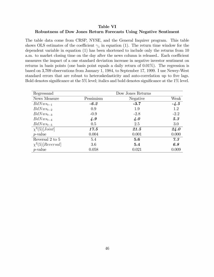
Table VIRobustness of Dow Jones Return Forecasts Using Negative Sentiment
The table data come from CRSP, NYSE, and the General Inquirer program. This tableshows OLS estimates of the coefficient γ1 in equation (1). The return time window for thedependent variable in equation (1) has been shortened to include only the returns from 10a.m. to market closing time on the day after the news column is released.. Each coefficientmeasures the impact of a one standard deviation increase in negative investor sentiment onreturns in basis points (one basis point equals a daily return of 0.01%). The regression isbased on 3,709 observations from January 1, 1984, to September 17, 1999. I use Newey-Weststandard errors that are robust to heteroskedasticity and auto-correlation up to five lags.Bold denotes significance at the 5% level; italics and bold denotes significance at the 1% level.
Regressand Dow Jones ReturnsNews Measure Pessimism Negative WeakBdNwst−1 -6.2 -3.7 -4.5BdNwst−2 0.9 1.9 1.2BdNwst−3 -0.9 -2.8 -2.2BdNwst−4 4.9 4.0 5.3BdNwst−5 0.5 2.5 3.0χ2(5)[Joint] 17.5 21.5 24.0p-value 0.004 0.001 0.000Reversal 2 to 5 5.4 5.6 7.3χ2(5)[Reversal] 3.6 5.4 6.8p-value 0.058 0.021 0.009
46

Table VIIRobustness of Log NYSE Volume Forecasts Using Sentiment
The table data come from CRSP, NYSE, and the General Inquirer program. This tableshows OLS estimates of the coefficient γ3 in equation (3). The definition of volume inequation (3) has been modified to include only trades occurring between 10 a.m. and marketclosing time on the day after the news column is released. The two sets of coefficientsdescribe the impact of one standard deviation increases in negative sentiment and theabsolute value of sentiment on detrended log NYSE volume growth. The regression is basedon 3,709 observations from January 1, 1984, to September 17, 1999. I use Newey-Weststandard errors that are robust to heteroskedasticity and auto-correlation up to five lags.Bold denotes significance at the 5% level; italics and bold denotes significance at the 1% level.
Regressand VolumeNews Measure Pessimism Negative WeakBdNwst−1 -0.52 0.01 -0.49BdNwst−2 -0.07 -0.09 0.22BdNwst−3 0.43 -0.49 0.88BdNwst−4 -0.12 0.42 1.01BdNwst−5 0.08 0.38 0.14|BdNwst−1| 1.17 1.51 1.34|BdNwst−2| -1.52 -0.43 -0.16|BdNwst−3| 0.01 0.42 -0.33|BdNwst−4| 1.02 0.51 0.42|BdNwst−5| -1.88 0.13 -0.63χ2(5) [BdNws] 3.2 2.0 14.1p-value 0.676 0.852 0.015χ2(5) [|BdNws|] 31.8 12.0 8.4p-value 0.000 0.035 0.137
47

Table VIIIRobustness of SMB Return Forecasts Using Negative Sentiment
The table data come from CRSP, NYSE, Professor Kenneth French’s web site and theGeneral Inquirer program. This table shows OLS estimates of the coefficient γ4 in equation(4); however, equation (4) has been modified to include the second through sixth lags ofthe pessimism factor rather than the first through fifth lags. Each coefficient measuresthe impact of a one standard deviation increase in negative investor sentiment on returnsin basis points (one basis point equals a daily return of 0.01%). The regression is basedon 3,709 observations from January 1, 1984, to September 17, 1999. I use Newey-Weststandard errors that are robust to heteroskedasticity and auto-correlation up to five lags.Bold denotes significance at the 5% level; italics and bold denotes significance at the 1% level.
Regressand Small-Minus-Big ReturnsNews Measure Pessimism Negative WeakBdNwst−2 0.2 -1.1 -1.2BdNwst−3 -0.8 -0.0 -0.0BdNwst−4 -2.8 -2.7 -3.0BdNwst−5 -1.3 -2.0 -2.3BdNwst−6 -2.0 -1.0 -1.6χ2(5)[Joint] 14.3 16.6 16.6p-value 0.014 0.005 0.005Sum 2 to 6 -6.7 -6.8 -8.0χ2(1)[Sum] 9.7 14.8 13.8p-value 0.002 0.000 0.000
48

Table IXPredicting Dow Jones Returns Using Negative Sentiment
The table data come from CRSP, NYSE, and the General Inquirer program. This tableshows OLS estimates of the coefficient γ1 in equation (1). Each coefficient measures theimpact of a one standard deviation increase in negative investor sentiment on returns inbasis points (one basis point equals a daily return of 0.01%). Each regression is basedon 3,709 observations from January 1, 1984 to September 17, 1999. I use Newey-Weststandard errors that are robust to heteroskedasticity and auto-correlation up to 5 lags. Bolddenotes significance at the 5% level; and italics and bold denotes significance at the 1% level.
Regressand Dow Jones ReturnsTime Period 1984—1991 1992—1999News Measure Pessimism Negative Weak Pessimism Negative WeakBdNwst−1 -0.5 3.1 -0.1 -13.6 -10.9 -9.8BdNwst−2 -3.7 0.7 -1.2 3.3 5.8 3.3BdNwst−3 -2.3 -3.1 -2.8 2.4 -2.3 -0.5BdNwst−4 6.7 5.0 9.3 3.1 3.4 4.6BdNwst−5 -2.8 2.6 2.7 2.9 2.6 3.8χ2(5)[Joint] 5.9 9.3 9.3 42.2 31.1 28.3p-value 0.316 0.099 0.098 0.000 0.000 0.000Sum of 2 to 5 -2.1 5.2 8.0 11.7 9.5 11.3χ2(1)[Reversal] 0.2 1.4 1.8 6.7 10.7 7.2p-value 0.681 0.234 0.183 0.010 0.018 0.007
49

Figure 1. Impact of a negative sentiment shock on prices. The graph depicts thetheoretical impact of a one-time increase in negative investor sentiment on equity prices. Ifthe media pessimism measure is a predictor of investor sentiment, it will predict low short-horizon returns followed by high long-horizon returns of approximately equal magnitude. Ifthe media pessimismmeasure follows past investor sentiment, it will predict low short-horizonreturns followed by high long-horizon returns of greater magnitude than the short-horizonreturns.
50

Figure 2. The effect of negative sentiment on Dow Jones returns. Data fromauthor’s application of the General Inquirer program to the Wall Street Journal columnfrom January 2, 1984, to September 17, 1999. The Dow Jones residuals come from theregression depicted in equation (1). The three measures of negative sentiment are calculatedusing the factor analysis procedure described in Section III. In the original unsmoothed data,there are 3,709 observations on daily residual Dow Jones returns and negative sentiment.Each smoothed data point represents the fitted value from a locally weighted least squaresregression of residual Dow Jones returns on negative sentiment. In each local regression,I apply local weightings from the standard tricube weighting function to only neighboringvalues of negative sentiment. The neighborhood for each data point is centered around thedata point and includes one half of the sample.
51