Gillies, E.A. and Cannon, R.M. and Green, R.B. and Pacey ...eprints.gla.ac.uk/6249/1/6249.pdf ·...
31
Gillies, E.A. and Cannon, R.M. and Green, R.B. and Pacey, A.A. (2009) Hydrodynamic propulsion of human sperm. Journal of Fluid Mechanics, 625 . pp. 445-474. ISSN 0022-1120 http://eprints.gla.ac.uk/6249/ Deposited on: 19 April 2010 Enlighten – Research publications by members of the University of Glasgow http://eprints.gla.ac.uk
Transcript of Gillies, E.A. and Cannon, R.M. and Green, R.B. and Pacey ...eprints.gla.ac.uk/6249/1/6249.pdf ·...

Gillies, E.A. and Cannon, R.M. and Green, R.B. and Pacey, A.A. (2009) Hydrodynamic propulsion of human sperm. Journal of Fluid Mechanics, 625 . pp. 445-474. ISSN 0022-1120
http://eprints.gla.ac.uk/6249/ Deposited on: 19 April 2010
Enlighten – Research publications by members of the University of Glasgow http://eprints.gla.ac.uk

J. Fluid Mech. (2009), vol. 625, pp. 445–474. c© 2009 Cambridge University Press
doi:10.1017/S0022112008005685 Printed in the United Kingdom
445
Hydrodynamic propulsion of human sperm
ERIC A. GILLIES1, R ICHARD M. CANNO N1,R ICHARD B. GREEN1 AND ALLAN A. PACEY2†
1Department of Aerospace Engineering, University of Glasgow, Glasgow G12 8QQ, UK2Academic Unit of Reproductive and Developmental Medicine,
School of Medicine and Biomedical Sciences, University of Sheffield, Sheffield S10 2SF, UK
(Received 19 February 2008 and in revised form 15 December 2008)
The detailed fluid mechanics of sperm propulsion are fundamental to our under-standing of reproduction. In this paper, we aim to model a human sperm swimmingin a microscope slide chamber. We model the sperm itself by a distribution ofregularized stokeslets over an ellipsoidal sperm head and along an infinitesimally thinflagellum. The slide chamber walls are modelled as parallel plates, also discretized bya distribution of regularized stokeslets. The sperm flagellar motion, used in our model,is obtained by digital microscopy of human sperm swimming in slide chambers. Wecompare the results of our simulation with previous numerical studies of flagellarpropulsion, and compare our computations of sperm kinematics with those of theactual sperm measured by digital microscopy. We find that there is an excellentquantitative match of transverse and angular velocities between our simulations andexperimental measurements of sperm. We also find a good qualitative match oflongitudinal velocities and computed tracks with those measured in our experiment.Our computations of average sperm power consumption fall within the range obtainedby other authors. We use the hydrodynamic model, and a prototype flagellar motionderived from experiment, as a predictive tool, and investigate how sperm kinematicsare affected by changes to head morphology, as human sperm have large variabilityin head size and shape. Results are shown which indicate the increase in predictedstraight-line velocity of the sperm as the head width is reduced and the increasein lateral movement as the head length is reduced. Predicted power consumption,however, shows a minimum close to the normal head aspect ratio.
1. IntroductionAn understanding of the fluid mechanics of sperm propulsion is fundamental to
our understanding of the biology of reproduction (Fauci & Dillon 2006). This fluidflow may be approximated by the inertialess Stokes equations (Gray & Hancock1955), where the cell is propelled by zero-thrust swimming (Lighthill 1976).
Many previous studies of flagellar propulsion have used spermatozoa as anarchetype. Taylor (1951) began the first quantitative analyses of swimming micro-organisms by assuming the flagellum as a two-dimensional, small amplitude sheet.More realistic geometries, including models with high amplitude, thin flagella, weredeveloped by Hancock (1953), who placed a distribution of stokeslets and doublets,singular solutions to the Stokes equations, along the flagellum centreline. This
† Email address for correspondence: [email protected]
446 E. A. Gillies, R. M. Cannon, R. B. Green and A. A. Pacey
slender-body theory (SBT) approach did not account for a head attached to theflagellum. Gray & Hancock (1955) introduced resistive-force theory (RFT) wheretangential and normal resistance coefficients, Ct and Cn, proportional to the relativevelocity of an element of the flagellum, are derived using SBT for a given flagellar waveand thickness. Integration of these coefficients gives a flagellar propulsive force andmoment that, when taken in conjunction with cell tangential and normal drag, allowcalculation of the propulsive velocity of the cell. This early model was used by manyresearchers in studying sperm propulsion (see Brennen & Winet 1977). Brokaw (1970)used RFT to analyse arbitrary planar motions of a sperm tail and compared computedaverage propulsive velocities with those found in experiment. Brokaw (1970) wasperhaps the first to suggest using a series of photographs of cell position and flagellarmotion to compare computed cell trajectories with experiment. Yundt, Shack &Lardner (1975) carried out this suggestion by taking high-speed cinematography ofsea urchin, rabbit, and bull sperm, and used Brokaw’s modified RFT to computesperm tracks resulting from the observed tail motions. These computed trackswere compared to the observed tracks. The approach of Yundt et al. (1975) isthe one we update here using digital image processing and a stokeslet simulation.These SBT and RFT approaches have been thoroughly reviewed by Lighthill (1976)and Brennen & Winet (1977), and compared by Johnson & Brokaw (1979). Higdon(1979) developed an improved SBT incorporating an image system of the flagelluminside a spherical cell head – this exact approach accounted for the hydrodynamicinteraction between head and flagellum, which was missing from RFT. Higdon (1979)studied the effects of wavelength and amplitude changes of the flagellum (as didDresdner, Katz & Berger 1980) and also the effects of changing spherical headdimension on both power and propulsive velocity. Phan-Thien, Tran-Cong & Ramia(1987) introduced the boundary-element method (BEM) for flagellar propulsion toaccount for non-spherical heads and non-slender flagella. These researchers derivedoptimal geometrical configurations for micro-organisms using helical flagellar motion,based on propulsive velocity and dissipated power. Cortez, Fauci & Medovikov (2005)introduced the regularized stokeslet method as a way of removing singularities fromdistributions of stokeslets and applied this to both BEM and infinitesimally thinflagella. An advantage of the regularized method is that it gives a bounded velocityfield for simulations like ours where the head is modelled as a smooth surface and theflagellum by a simple line filament, or for simulations where the stokeslets distributedas a set of discrete, disconnected, points such as might be used to model a largenumber of suspended micro-organisms (Cisneros et al. 2007).
Many researchers have highlighted the significant effects of the presence of solid(or fluid) boundaries (Brenner 1962; Rothschild 1963; Blake 1971; Blake & Chwang1974; Katz 1974; Fulford & Blake 1983; Gueron & Liron 1992; Ramia, Tullock &Phan-Thien 1993) on the motion of spheres, slender bodies, fixed cilia or swimmingmicro-organisms at low Reynolds number. One of the first studies to take into accountthe effect of solid boundaries on flagellar propulsion was Reynolds (1965) who usedthe early flagellum model of Taylor (1951) in the presence of a wall. Katz (1974)showed that an important feature of flagellar propulsion near a plane boundary wasan increase in the ratio of normal to tangential resistance coefficients. Given that itis this ratio which determines flagellar propulsive force in RFT, and the values of thecoefficients which determine power dissipation, this work suggested that the presenceof walls must be included when considering cells observed between a microscopeslide and coverslip. There are also many instances in the female reproductive tractwhere sperm are in close proximity to epithelial surfaces, or the ovum (Fauci & Dillon

Hydrodynamic propulsion of human sperm 447
2006). Ramia et al. (1993) undertook a thorough study of the effects of both a singlewall, modelled by an image system, and parallel plates, modelled by an image systemand discretized plate, on the locomotion of a swimming microorganism. Ramia et al.(1993) also undertook simulations of interactions between close swimming micro-organisms, as did Ishikawa et al. (2007), both using a BEM formulation. Recently,Cisneros et al. (2007) and Ainley et al. (2008) have applied the method of regularizedstokeslets to flows bounded by a single wall, and Cisneros et al. (2007) to simulationsof multiple interacting organisms.
Most previous studies of flagellar propulsion have, with the exception of Yundtet al. (1975) and Dresdner & Katz (1981), used prototype travelling waves to modelthe flagellar beat. Yundt et al. (1975) used high-speed cinematography to manuallytrace out actual flagellar beat and cell kinematics and compared these to predictionsof cell kinematics using resistive-force theory. A significant technological advancesince the work of Yundt et al. (1975) has been the advent of high frame rate digitalvideo cameras that can be coupled with microscopy to obtain images of the flagellumthroughout many flagellar beat cycles. In this paper, we use digital microscopy tomeasure approximate head morphology, kinematics and actual flagellar beat, on anumber of sperm and compare the measured kinematics to those computed using adistribution of regularized stokeslets (Cortez et al. 2005) that discretize the sperm.The method of regularized stokeslets is appropriate as we model the sperm head asa discretized ellipsoidal surface and the flagellum as a slender filament. In addition,we follow Ramia et al. (1993) by noting that the effects of the microscope slide andcoverslip walls are likely to be significant, given that the chambers used in clinicalandrology are usually 20 μm deep, which is around half the length of the sperm. Theresults of Fulford & Blake (1983); Katz (1974); Ramia et al. (1993), amongst others,indicate the Ct/Ct∞ and Cn/Ct ratios for rods translating parallel to and midwaybetween slide chamber walls. Here, Ct∞ is the tangential resistance coefficient in aninfinite medium. For a 50 μm long slender rod, similar to the size of a human spermflagellum (WHO 1999), these results indicate ratios of Ct/Ct∞ ≈ 1.18 and Cn/Ct ≈ 1.78for a 50 μm deep chamber, and Ct/Ct∞ ≈ 1.39 and Cn/Ct ≈ 2.09 for a 20 μm deepchamber (values obtained by reading the BEM results in figure 4(e) of Ramia et al.1993). We therefore also discretize the microscope slide chamber in our simulations.
The paper begins with a discussion of our hydrodynamic solution method fora flagellum and attached cell body, and verification of the computational methodon translating sphere and rod test cases, as well as comparison with the propulsivevelocity calculations of Dresdner et al. (1980) and Higdon (1979) and dissipatedpower calculations of Higdon (1979). We then introduce the walls of the microscopeslide chamber into the simulation, and verify these calculations against the resultssummarized in Ramia et al. (1993). The paper proceeds with a calculation ofpropulsive velocity and trajectory, resulting from experimentally observed flagellarmotions, and a comparison of these kinematics with experiment. In addition to usingexperimentally observed sperm for validation of the hydrodynamic code, we discusspredictions of sperm power dissipation. Finally, we use our method to predict changesto sperm kinematics and power consumption that result from hydrodynamic effectsof changes to head geometry.
2. Hydrodynamic simulation methodMammalian sperm, including those of humans, exhibit various swimming
behaviours throughout their life, which are thought to be related to the different

448 E. A. Gillies, R. M. Cannon, R. B. Green and A. A. Pacey
stages of their journey through the female reproductive tract (Suarez & Pacey 2006).Briefly, following ejaculation, sperm motion is initially linear and progressive; whereasonce sperm reach the uterine (fallopian) tubes, their pattern of movement changesto become more erratic and hyperactivated. While hyperactivated motility is thoughtto be important in the final stages of fertilization, this paper will examine the fluidmechanics of progressively motile sperm, since these are what are evaluated in semenanalysis (WHO 1999) to determine the sperm that are capable of penetrating cervicalmucus and therefore capable of entering the female reproductive tract (Aitken et al.1985). The motile concentration of such sperm has been shown to be closely associatedwith predicting the probability of conception (Larsen et al. 2000).
The length of the human sperm flagellum L is around 50 μm (WHO 1999) and itsradius a is 0.25 μm (Dresdner & Katz 1981); the head is approximately an ellipsoidof 5.8 × 3.1 × 1 μm (Brennen & Winet 1977) – although human sperm display alarge variability in head morphology. The straight line, propulsive velocity of spermisolated from seminal plasma by density centrifugation and then observed in a simplesalt solution is around 40–100 μms−1 (Mortimer 1994). The viscosity of semen isvariable (Owen & Katz 2005), but for experiments in tissue culture, the fluid hasa viscosity close to water at 37 ◦C. The Reynolds number of the sperm cell duringprogressive motility is therefore of the order of 10−2 (Dresdner et al. 1980).
Given the very low Reynolds number, the inertialess Stokes equations are a usefulapproximation for the flow (Happel & Brenner 1981; Lighthill 1976). We define alocal coordinate frame x–y, with x aligned along the head principal axis and theundeformed flagellum. The centre of this frame is the head centroid. We also definea fixed global frame X–Y. The unknown swimming velocity of the sperm is, in thelocal coordinate frame aligned with the head, Up(t), and its angular velocity, Ω(t).The head and flagellum are parameterized by position r(s, t), where s is a coordinateon the surface of the cell. The flagellum has ‘beat’ velocity u(s, t), but the head doesnot beat. For planar motion of the cell (Brennen & Winet 1977), the velocity at anypoint on the cell is
u(s, t) = u(s, t) + Up(t) + Ω × r(s, t). (2.1)
The incompressible Stokes equations, pertinent to the flow, are
μ∇2u − ∇p = f , ∇ · u = 0. (2.2)
As the Stokes equations are inertialess, they do not admit accelerations. Consequently,the force f (s, t) and moment generated by the cell have to balance∫
s
f ds = 0,
∫s
r × f ds = 0, (2.3)
where the integrals are over the entire surface of the cell (head, mid-piece andflagellum). This force balance is termed zero-thrust swimming (Lighthill 1976).
At each time point during a numerical simulation, this force balance is used toderive the unknown propulsive velocity that results from the flagellar motion. TheStokes equations are steady (Happel & Brenner 1981), but the propulsive velocityrequired for a force balance at any instant will vary with the instantaneous flagellarposition and velocity. In this way the steady, inertialess Stokes equations can beused to calculate sperm acceleration. The zero force and moment balances are anintegral part of the fluid solution procedure. This procedure generates a time-varyingpropulsive velocity, which can then be used to reconstruct the cell track, and a

Hydrodynamic propulsion of human sperm 449
time-varying force distribution, which may be used, via an application of the Stokesequations throughout the flow-field, to obtain the fluid flow-field velocities.
2.1. Method of regularized stokeslets
In order to solve the Stokes equations we use a very useful approximation of theregularized stokeslet due to Cortez (2001): the (unknown) velocity at any point s overthe sperm cell surface is
uj (s) = − 1
8πμ
N∑n=1
3∑i=1
Sij (sn, s)fn,iAn, (2.4)
where it is assumed that the cell has been discretized into N points, An is acorresponding quadrature weight (which may vary depending on whether the pointis on the head, mid-piece or the flagellum), and −fn,i is the ith component of theforce on the fluid applied at point n, which is an unknown. Sij (sn, s) is the regularizedstokeslet of Cortez (2001), which removes the singularity of the stokeslet.
Sij (sn, s) = δij
r2 + 2ε2
(r2 + ε2)3/2+
(xi(sn) − xi(s))(xj (sn) − xj (sn))
(r2 + ε2)3/2(2.5)
with r = ||x(sn) − x(s)||, and ε a small regularization parameter. The optimum value ofε is one which minimizes the velocity, or force, error for a particular discretization ofthe surface geometry (Ainley et al. 2008) and may be different between the head andflagellum (and walls if present). Choice of the regularization parameter is intimatelyinvolved with the choice of discretization and is discussed in § 2.2. In vector form,(2.4) is
u = G f . (2.6)
The problem is three-dimensional, with six unknowns (three translational andthree rotational propulsive velocities) but only propulsive motion in the x–y planeis non-zero in our simulations: the tail motion is restricted to this x–y plane, andthe problem is symmetrical about z = 0 as we simulate sperm swimming in either aninfinite medium, or parallel to, and mid-way between parallel slide chamber walls. Foreach point on the cell, and on the slide chamber walls (if present), the velocity is splitinto a known beat velocity, zero-velocity boundary condition or component resultingfrom the unknown cell propulsive velocity. For planar motion, each cell point i hasthe x and y components of propulsive velocity (including angular velocity),
XiUp, (2.7)
where
Xi =
[1 0 −ryi
0 1 rxi
0 0 0
](2.8)
and Up = [Upx Upy Ω]T . Concatenated into a vector comprising all the discrete pointsin the problem (i.e. on the cell head, flagellum and slide chamber walls), the velocity-boundary condition is u = u + XUp . Matrix G is inverted and we form the vectors
b = G−1u; a = −G−1X. (2.9)
The x, y components of the vectors b, a and the z component of r × b, r × a areintegrated over the surface of the cell to give B, the components of force and momentresulting from the beat velocity, and A, the components of force resulting from the
450 E. A. Gillies, R. M. Cannon, R. B. Green and A. A. Pacey
(a)
(b) (c)
0.1 0.2 0.3 0.4 0.5 0.6 0.7 0.8 0.910–3
10–2
10–1
100
Regularization parameter ε/ds
Cum
ula
tive
erro
r dis
trib
uti
on
||e|| L
2 d
rag e
rror
1.0
0.9
0.8
0.7
0.6
0.5
0.4
0.3
0.2
0.1
0 0.01
Velocity error of non-collocation point i: ei = |Uxi –1|
0.02 0.03 0.04 0.05
StokesletNon-collocationpoint
0.06
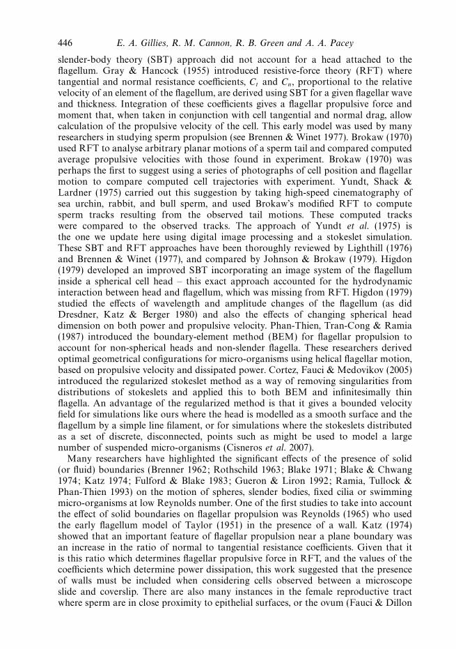
Figure 1. (a) Discretization of the head and flagellum (inset box shows the head in close-up).The dots are stokeslet positions. (b) L2 regularization error for translating, head-shapedellipsoids and ‘flagella-like’ rods. (c) Cumulative distribution of local velocity error fornon-collocated points on the surface of a translating sphere. Collocated and non-collocatedpoints are shown in the inset figure with an arrow showing the translation direction.
unknown propulsive velocity. As these forces and moments on the cell integrate tozero, finally, Up is found from solution of
AUp = B. (2.10)
2.2. Spatial discretization, and regularization parameter for a free-swimming sperm
Normal sperm are comprised of three distinct structural regions: the head, mid-pieceand the flagellum. In our experiments, the mid-piece was difficult to distinguish fromthe proximal end of the flagellum, so, for the purposes of hydrodynamic simulation,we modelled the sperm with an ellipsoidal head and thin flagellum only. The methodof regularized stokeslets may be applied to both infinitesimally thin flagella andspherical/ellipsoidal bodies, allowing us to investigate both the effects of tail beat andhead morphology on the cell’s fluid mechanics.
A human sperm head is, very approximately, a scalene ellipsoid (Brennen & Winet1977), and it is computationally expedient to discretize the surface of the head by astrip, arranged in a spiral from the front of the head to the back (see figure 1a), muchlike an apple peel. In this way, a single coordinate s can be used to label points overthe head (along the head ‘peel’) and along the flagellum. Alternative discretizationsare also possible (Cortez et al. 2005), and we made sure that our simulations werenot dependent on the discretization. The quadrature weights for the head are thusds × p, where p is the peel thickness. A standard head dimension of 5.8 × 3.1 × 1 μm

Hydrodynamic propulsion of human sperm 451
was used for validating our hydrodynamic simulation, but, in general, sperm maypresent a range of length/width ratios, some of which may be considered abnormalfor clinical purposes by the relatively strict definition provided by WHO (1999). Inour discretization, we keep the absolute size of ds and p the same, so that the areaof each element on the head stays the same, regardless of head dimensions. The totalnumber of patches on each modelled sperm head is therefore proportional to thehead surface area. In this way we had a consistent method of discretizing heads of arange of dimensions (including a range of possible human sperm head morphologiesand also spheres for comparison with the results of Ramia et al. 1993 and Higdon1979). For our simulations, a step size ds = 0.7 μm was chosen, and the thickness p
was set at ds/4 so that the standard head dimension was discretized by 101 points.The discretization is such that each stokeslet force acts over approximately the samepatch area on the head. Constant force discretization was used.
The natural way to discretize the flagellum, given that it is a thin, approximatelyinextensible filament is a series of equally spaced points along the flagellum. The forceand moment balance for the flagellum, as an integral along a filament, has quadratureds. The flagellum thickness of 0.5 μm only enters the computation in the choice ofoptimum regularization parameter ε, which is discussed below.
With this fixed discretization for all spheres, ellipsoidal heads and flagella that wewished to model, we were able to investigate an appropriate regularization parameterfor the stokeslets on the cell. There is an optimum regularization parameter, whichwill give a minimum force, or velocity, error for a particular discretization (Ainleyet al. 2008). Following the approach of Ainley et al. (2008) and Cortez et al. (2005),it is reasonable to choose a regularization parameter based on known exact resultswhich are closely related to the problem at hand. To this end, we examined ourpredictions of drag on ellipsoids (of a range of dimensions similar to those of humansperm heads) and of thin rods (of a dimension similar to sperm flagella) translatingin x and y directions in an infinite medium. We also studied the drag on spheres ofa large range of sizes (larger than the range of sizes expected to be observed in ahuman ejaculate). The rods were modelled in the same way as the flagellum, and theirexact solution was based on that of an elongated, needle-like ellipsoid (Happel &Brenner 1981). Figure 1(b) shows the L2 error for all of the ellipsoid, sphere and roddrag simulations as the regularization parameter is varied. The L2 error is defined as
||e||L2=
√√√√ 1
M
1
D2max
M∑i=1
e2i
with the error ei = D − Do, where D is the predicted drag force on the ellipsoid orrod, and Do is the associated theoretical drag. While Dmax is the maximum valueof theoretical drag, M is the number of separate simulations used to optimize theerror. We chose two isolated rod simulations (one longitudinal and one transversetranslation) and two isolated ellipsoid simulations (both with an ellipsoid of dimension5.8 × 3.1 × 1 μm, with one longitudinal and one transverse translation) to plotfigure 1(b). The optimum ε = 0.32 did not change when we varied the ellipsoiddimensions. This value is fixed for our particular discretization and is kept constantin all of our simulations.
Singular stokeslets alone may be used to model the flow around a cell body such asa sperm head by, for example, the highly accurate boundary-integral method. For theflagellum, a line distribution of singular stokeslets may not be sufficiently accurate
452 E. A. Gillies, R. M. Cannon, R. B. Green and A. A. Pacey
tf
(a)
UP
x/c
; (b
) U
Py/
c ;
(c) θ
(b)
(a)
(c)
Dresdner et al. (1980)
Computation
0 0.2 0.4 0.6 0.8 1.0–0.8
–0.6
–0.4
–0.2
0
0.2
0.4
0.6
0.8
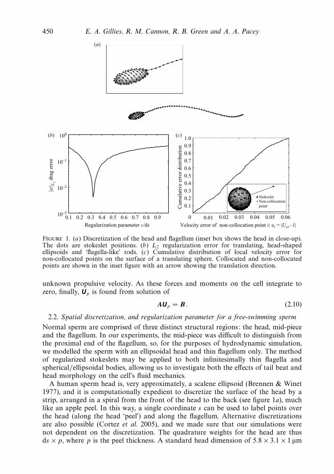
Figure 2. Computed temporal variation of (a) UPX/c, (b) UPY /c and (c) θ for a headlessflagellum of shape given by y = α sin k(x − ct) with αk =1, n= 1, over a beat cycle comparedwith the results of Dresdner et al. (1980).
to represent the flow around the slender-body and higher-order singularities may berequired to give the desired accuracy in the near field. For example, see Dresdneret al. (1980) where the near field of the flagellum was modelled by stokeslets andstokes doublets but the far-field by stokeslets alone. The regularized stokeslet method,which we use here, causes each force to be spread over a small, smooth sphere ratherthan a single point (Cortez et al. 2005): this ensures that the near-field velocity erroris small without recourse to higher-order singularities, such as Stokes doublets anddipoles. The cumulative local velocity error at non-collocated points, ei = |Uxi − 1| fora sphere, with i = 1, . . . , 500, translating with velocity Ux = 1 is plotted in figure 1(c).Fifty per cent of these 500 non-collocated points have error less than 2.7 %, 90 % haveerror less than 5.0 %, and all have an error less than 6 %. Discretization and a choiceof regularization parameter of the microscope slide chamber walls are discussed in§ 2.4.
2.3. Verification of the free-swimming sperm model
The free-swimming model was verified by comparison with two test cases priorto comparison with the kinematics of experimentally observed sperm: the workof Dresdner et al. (1980) who plotted time histories of propulsive velocities for afree-swimming headless flagellum and the work of Higdon (1979) who undertooka thorough theoretical, hydrodynamic study of the effects of head size on flagellarpropulsion and cell power consumption.
A comparison of the regularized stokeslet method with the results of Dresdner andKatz’s headless flagellum is shown in figure 2. For this test case, the flagellum has fixedinextensible length L, radius a, and the y coordinate is y(s) = α sin k(x(s) − ct), withαk = 1 and a/L = 0.01. The wavelength of the flagellar motion is L. The travellingwave flagellum is discretized by N = 50 equally spaced regularized stokeslets alongthe flagellum. The velocity of the flagellum at these points was calculated analytically.In figure 2 we compare our results to those in figure 3 of Dresdner et al. (1980). Theresults show dimensionless propulsive velocity (in a global frame) and the orientationof the longitudinal axis of the flagellum. The comparison between our results andthose of Dresdner et al. (1980) is shown to be generally very good.

Hydrodynamic propulsion of human sperm 453
0 0.02 0.04 0.06 0.08 0.10 0.12
0.05
0.10
0.15
0.20
0.25(a) (b)
Non-dimensional spherical head radius (A/L)
Inver
se e
ffic
iency
η–1
UP/c α k = 1.5
α k = 1.0
Higdon (1979)
Computation
Higdon (1979)
Computation
350
300
250
200
150
100
50
00.05 0.10
Spherical head size A/L0.15 0.20
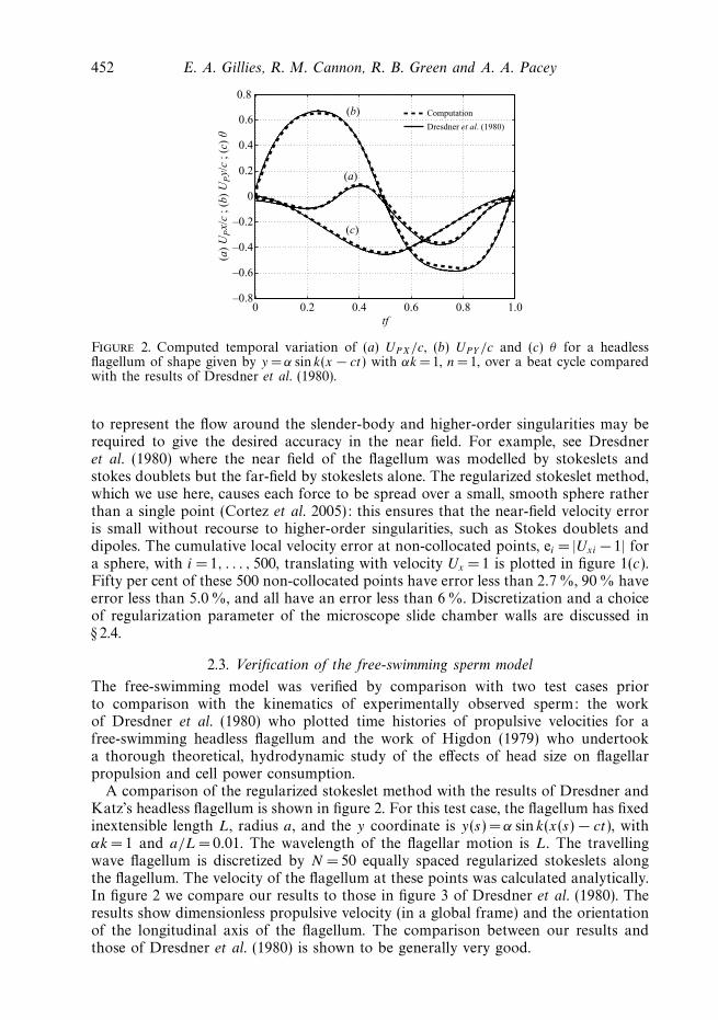
Figure 3. (a) Normalized average straight-line velocity Up/c computed for a range of sphericalhead radius A/L values. Flagellar beat is a radially attached sinusoidal travelling wave. Crossesare results extracted from figure 5 of Higdon (1979), which compare well with our results(solid lines) using regularized stokeslets. (b) Predicted non-dimensional inverse efficiency η−1
for cells with a range of head size A/L and flagellar radius 0.01L. Crosses are results extractedfrom figures 6 and 14 of Higdon (1979), which compare well with our results (solid lines) usingregularized stokeslets.
To verify our prediction of the effect of head size on cell kinematics and powerconsumption we compare with the results of Higdon (1979). Higdon considered adistribution of stokeslet and dipole singularities along a helical, or planar, flagellarcentreline, a stokeslet, dipole, and rotlet to model a spherical head, with an imagesystem for the flagellum singularities at the spherical cell body centre. The flagellarwave studied by Higdon was a single-frequency travelling wave, attached radially tothe spherical cell body. The range of spherical head sizes considered by Higdon rangedfrom A/L = 0.05 to A/L = 0.2. The smaller head sizes studied by Higdon approachthe dimensions found in many species of spermatozoa – for example, human sperm,with dimension close to that of an ellipsoid of 5.8 × 3.1 × 1 μm have a volumeequivalent radius of 2.6 μm, which with a flagellar length of 50 μm is A/L = 0.052.The longitudinal, translational, equivalent radius (Happel & Brenner 1981) for suchan ellipsoid is 1.39 μm, giving A/L = 0.028. The same geometry was used as an inputto our code, with the sperm head and flagellum discretized by regularized stokeslets,rather than by Higdon’s exact method. This verification was necessary to show thatour model could predict propulsive velocity as head morphology was varied.
Data read from Higdon’s figure 5 were recast into a graph of spherical headradius A, non-dimensionalized by tail length L, versus straight line swimming speedUp , non-dimensionalized by wave speed c, and shown in figure 3(a). The flagellumwave amplitude is α, and with fixed wavenumber k =2π/L, the parameter αk is non-dimensional amplitude. Two different values of this amplitude parameter αk =1, 1.5,and a range of head sizes between headless and 0.10L were investigated. Thetwo different computational methods reveal similar results, with Higdon’s resultsrepresented as crosses, and our computations by solid lines in figure 3(a). Weconcluded that our model could adequately predict the hydrodynamic effects ofchanging head size.
Higdon (and Phan-Thien et al. 1987) also calculated dimensionless inverse efficiency
η−1 =P
(6πμA + KT L)U 2, (2.11)
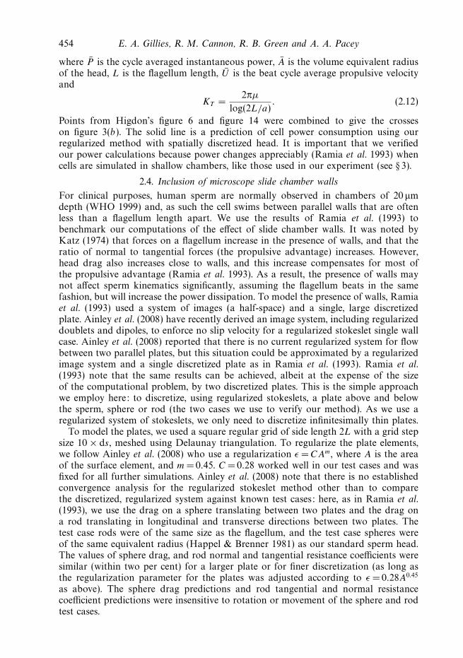
454 E. A. Gillies, R. M. Cannon, R. B. Green and A. A. Pacey
where P is the cycle averaged instantaneous power, A is the volume equivalent radiusof the head, L is the flagellum length, U is the beat cycle average propulsive velocityand
KT =2πμ
log(2L/a). (2.12)
Points from Higdon’s figure 6 and figure 14 were combined to give the crosseson figure 3(b). The solid line is a prediction of cell power consumption using ourregularized method with spatially discretized head. It is important that we verifiedour power calculations because power changes appreciably (Ramia et al. 1993) whencells are simulated in shallow chambers, like those used in our experiment (see § 3).
2.4. Inclusion of microscope slide chamber walls
For clinical purposes, human sperm are normally observed in chambers of 20 μmdepth (WHO 1999) and, as such the cell swims between parallel walls that are oftenless than a flagellum length apart. We use the results of Ramia et al. (1993) tobenchmark our computations of the effect of slide chamber walls. It was noted byKatz (1974) that forces on a flagellum increase in the presence of walls, and that theratio of normal to tangential forces (the propulsive advantage) increases. However,head drag also increases close to walls, and this increase compensates for most ofthe propulsive advantage (Ramia et al. 1993). As a result, the presence of walls maynot affect sperm kinematics significantly, assuming the flagellum beats in the samefashion, but will increase the power dissipation. To model the presence of walls, Ramiaet al. (1993) used a system of images (a half-space) and a single, large discretizedplate. Ainley et al. (2008) have recently derived an image system, including regularizeddoublets and dipoles, to enforce no slip velocity for a regularized stokeslet single wallcase. Ainley et al. (2008) reported that there is no current regularized system for flowbetween two parallel plates, but this situation could be approximated by a regularizedimage system and a single discretized plate as in Ramia et al. (1993). Ramia et al.(1993) note that the same results can be achieved, albeit at the expense of the sizeof the computational problem, by two discretized plates. This is the simple approachwe employ here: to discretize, using regularized stokeslets, a plate above and belowthe sperm, sphere or rod (the two cases we use to verify our method). As we use aregularized system of stokeslets, we only need to discretize infinitesimally thin plates.
To model the plates, we used a square regular grid of side length 2L with a grid stepsize 10 × ds, meshed using Delaunay triangulation. To regularize the plate elements,we follow Ainley et al. (2008) who use a regularization ε = CAm, where A is the areaof the surface element, and m = 0.45. C = 0.28 worked well in our test cases and wasfixed for all further simulations. Ainley et al. (2008) note that there is no establishedconvergence analysis for the regularized stokeslet method other than to comparethe discretized, regularized system against known test cases: here, as in Ramia et al.(1993), we use the drag on a sphere translating between two plates and the drag ona rod translating in longitudinal and transverse directions between two plates. Thetest case rods were of the same size as the flagellum, and the test case spheres wereof the same equivalent radius (Happel & Brenner 1981) as our standard sperm head.The values of sphere drag, and rod normal and tangential resistance coefficients weresimilar (within two per cent) for a larger plate or for finer discretization (as long asthe regularization parameter for the plates was adjusted according to ε =0.28A0.45
as above). The sphere drag predictions and rod tangential and normal resistancecoefficient predictions were insensitive to rotation or movement of the sphere and rodtest cases.

Hydrodynamic propulsion of human sperm 455
0 2 4 6 8 10
0.5
1.0
1.5
2.0
2.5
3.0
3.5
4.0(a) (b)
h/A
F/F
∞
Half-depth range of MicrocellTM chambers
BEM Ramia et al. (1993)Computation
0 0.2 0.4 0.6 0.8 1.0
0.5
1.0
1.5
2.0
2.5
3.0
3.5
4.0
h/L
Half-depth range of MicrocellTM chambers
Cn /Ct Computation
Cn /Ct BEM Ramia et al. (1993)
Ct /Ct∞ Computation
Ct /Ct∞ BEM Ramia et al. (1993)
Figure 4. (a) Predicted increase in drag for spheres translating between parallel chamberwalls. The chamber half-depth is h and A is sphere radius. Square markers indicate the resultsof Ramia et al. (1993), and the solid line with cross (×) markers indicates our computationswith spheres. (b) Predicted increase in Ct/Ct∞ and Cn/Ct with varying chamber depth for arod mid-way between chamber walls. The chamber half-depth is h and the rod length is L.Square markers indicate the Ct/Ct∞ results; circle markers indicate the Cn/Ct results of Ramiaet al. (1993); the solid line with cross markers indicates our computations of Ct/Ct∞; and thesolid lines with plus (+) markers indicate our computations of Cn/Ct .
Figure 4(a) shows the ratio of predicted drag for a sphere translating between platesto the exact drag (6πμAU ) in an infinite medium. Our sphere simulation results areindicated by a solid line with cross markers. The results of Ramia et al. (1993)are shown as square markers in the figure. We only ran simulations which coverthe range of depths of microscope slide chamber encountered in our experiments(the half-depth of these MicrocellTM slides ranged from h = 6 μm to h = 25 μm in ourexperiments, which are detailed in the Appendix and discussed in § 3) and this rangeof depths is indicated in the figure. The comparison with the results of Ramia et al.(1993) is generally good over our range of interest.
Figure 4(b) shows our predictions of tangential and normal drag of a thin rod50 μm long and 0.5 μm wide over the range of chamber half-depths h encounteredin our experiments. The results are again compared to those of Ramia et al. (1993).We plot the ratio of tangential drag for the rod translating between plates to that ofa rod translating in an infinite medium, Ct/Ct∞. Following Ramia et al. (1993), wealso plot the ratio of normal to tangential resistance Cn/Ct . Our Ct/Ct∞ prediction isindicated by cross markers and a solid line and the corresponding results of Ramiaet al. (1993) by square markers. Our predicted Cn/Ct ratio is represented by plusmarkers and a solid line, and the corresponding results of Ramia et al. (1993) bycircle markers. The agreement is generally good with a slight underprediction ofCt/Ct∞, and a consequent over-prediction of Cn/Ct ratio at shallow chamber depths.Overall, the same drag trends with increasing drag and a greater increase in flagellarpropulsive advantage are shown with decreasing chamber depth.
3. Comparison of observed sperm kinematics with hydrodynamic predictionTo compare the results of our hydrodynamic code with the kinematics of sperm
observed in vitro we took digital images of several sperm (three are described inthis study) and measured both sperm head centroid position and flagellar position,which was used via numerical differentiation to estimate flagellar beat velocity. The

456 E. A. Gillies, R. M. Cannon, R. B. Green and A. A. Pacey
depth of field of the optics in our experiment was 4 μm, and sperm were observedas close to mid-way between the slide chamber walls as was possible to determine inour experiment. This mid-chamber focal plane was obtained by focusing on the slidechamber bottom and top (determined by the sharpness of focus of small scratches),and halving the number of turns of the microscope focus control. It was necessaryto obtain clear images of the tail at a frame rate high enough that the tail positionand beat velocity could be inferred along s. In our data, the distal end of the tailwas sometimes difficult to identify clearly. However, in the majority of images, thetail was clearly focused and defined for its entire length, allowing us to define L andcurve-fit a filament, length L, to the minority of images with out of focus or difficultto delineate tail images. In this way, we obtained tail position and beat velocity over acontinuous time period. Head dimensions were traced out manually using the clearestimages of the head. The head centroid position, and principal axis orientation werecalculated automatically. The technical limitations of observing tail movement shouldnot be underestimated: the system has to have images clear enough for accurate tailmorphology, and hence an appropriate camera exposure has to be set. To numericallydifferentiate position, the camera has to operate at a high enough frame rate. Thenominal beat frequency of human spermatozoa is around 10 Hz (Mortimer 1994)(although, in our experiments, we found this to vary significantly, and there wereusually at least two to three higher harmonics present). A Nyquist limit of at least60 Hz was judged to be the lowest possible frame rate, and this is possible usingmodern Computer-Aided Sperm Analysis (CASA) machines, but for the purposesof hydrodynamic analysis, this frame rate was doubled to at least 120 Hz to ensurethat the beat velocity estimates were accurate enough (the actual camera frame ratewas 121 Hz in our experiments). Details of the experimental method to obtain bothsperm kinematics and the position and beat velocity of the flagella are discussed inthe Appendix.
The beat velocity at point s, inferred from the time-varying flagellar position, isneeded to determine the force the flagellum exerts on the fluid at that point. This beatvelocity u(s, t) may be determined via the numerical time derivative of the position ofthe flagellum r(s, t) of each imaged sperm. A 4-point centred difference of recordedposition data was used to estimate the beat velocities. The raw data are at 121 Hzbut smaller time steps of 0.005 s were used in the hydrodynamic solution methodand so linear interpolation of the raw position and velocity was performed to obtainthe flagellum position and beat velocity at any required time point. As the beatvelocity is obtained via numerical differentiation of noisy position data, the predictedpropulsive velocities obtained by the hydrodynamic analysis are also contaminatedwith noise. Yundt et al. (1975) suggest comparing computed tracks with experiment,rather than just comparing computed propulsive velocity, as the integrated velocity isless sensitive to noise.
Three individual, progressively motile sets of cell kinematics are discussed here.Cells σ1 and σ3 were chosen for display as they are both long tracks, and σ2 waschosen because its track displays some ‘looping’ behaviour that we were intrigued tosee if the fluid mechanics analysis also predicted. Cells σ2 and σ3 were studied in 12 μmchambers, and were therefore expected to show significant effects of chamber walls,and σ1 in a 50 μm chamber. The effect of the chamber on σ1 was therefore expected tobe much less than for the shallower chambers. As well as simulations of spheres androds, Ramia et al. (1993) undertook simulation of micro-organisms swimming nextto walls and between parallel walls. Their results indicated that a flagellar propulsiveadvantage occurs when an organism swims close to walls, but that an increase in head

Hydrodynamic propulsion of human sperm 457
drag compensated for the propulsive advantage and so the cell propulsive velocitieswere not altered significantly. However, Ramia et al. (1993) pointed out that the powerrequirements for micro-organisms swimming between plates would be higher thanfor free swimming ones due to the increased forces on the head and flagellum. Weran the hydrodynamic simulation both with and without a model of the microscopeslide chamber walls to investigate how the prediction of sperm kinematics and powerconsumption was affected. Although there were sperm–sperm interactions in the dataset, σ1, σ2 and σ3 were sufficiently far away from other cells (generally greater than aflagellum length) for no contact to take place. There should have also been little effecton these cells from the local velocity fields generated by other swimming sperm, asthe velocity fields generated by a flagellum at this Reynolds number is only significantwithin a distance of the order of a flagellum length (Lighthill 1976). An exception wascell σ2 which passed within half a flagellum length of an immotile cell. No motion ofthis extra cell was noted however, so the force on σ2 was judged to be minimal.
The comparison is shown in terms of four sub-figures for sperm tracks σ1 andσ2. Sub-figure (a) shows the head orientation angle θ (which was integrated fromthe angular velocity), and sub-figures (b) and (c) show the propulsive velocities Upx
and Upy in the local coordinate frame aligned with the head. Sub-figure (d ) showsthe integrated absolute velocity giving the sperm centroid track. It is to be expectedthat the head orientation angle and computed track will drift from the observedexperimental data due to integrated errors. Following Yundt et al. (1975), we use acomparison of the predicted and experimental track as the most appropriate methodfor assessing the performance of the simulation. In addition to comparisons ofinstantaneous propulsive velocity and track, predicted power consumption for walledand unbounded simulations is plotted for each simulation. Only the track and powerconsumption comparison for the walled and unbounded simulations, are shown forcell σ3. A viscosity of μ = 0.001 Pa s was used in the simulations.
In figure 5, we show our simulation of sperm σ1 with and without the presenceof chamber walls and also the experimental kinematics for this cell. This cell wasprogressively motile and relatively fast. Its velocity along a 5-point running averagetrack, based on a 30 Hz data sample and defined as the VAP (Mortimer 1994), was105 μms−1, and the track length covered a period of 0.5 s. The head was approximatedby an ellipsoid of standard, 5.8 × 3.1 × 1 μm, dimension and the flagellar length wasmeasured as 41 μm. The results for simulated head angle and lateral velocity aregenerally very good. There are significant higher harmonic components above thebase beat cross frequency evident in both the experimental and simulated lateralvelocity. The simulation of local longitudinal velocity is slightly less good, with anotable loss of accuracy at 0.3–0.35 s. In general, the local longitudinal velocityprediction is much more sensitive to noise in the measured flagellar beat. For bothwalled and unwalled simulations, the integrated track displays the same transitionfrom ‘triangular-like’ waveform for the first two cycles of the track to a more ‘square-wave-like’ waveform. These same features are seen in the measured track and theshape of the track is quite well captured by the simulations. The dashed and solidlines are almost indistinguishable in figure 5(a–c), indicating that the simulation inthe deep chamber and in an unbounded medium result in very similar kinematics.This similarity is to be expected since the chamber is relatively deep. The forceson the flagellum and head are, however, slightly higher for the walled simulationthan for the simulation in an unbounded medium. These higher forces are evidentin figure 6, which shows the predicted power consumption of this sperm. In thisfigure, dashed lines represent the results of simulation in an unbounded medium, and

458 E. A. Gillies, R. M. Cannon, R. B. Green and A. A. Pacey
0 0.1 0.2 0.3 0.4
–80
–60
–40
–20
0
20
40
60
80H
ead a
ngle
θ
(a) (b)
(c) (d)
0 0.1 0.2 0.3 0.4–400
–300
–200
–100
0
100
200
300
400
UPx
(μm
s–1)
0 0.1 0.2 0.3 0.4–400
–300
–200
–100
0
100
200
300
400
Time along track (s)
Time along track (s) Time along track (s)
UPy
(μm
s–1)
–50 –40 –30 –20 –10 0
–10
–5
0
5
10
15
20
25
X track (μm)
Y t
rack
(μ
m)
Infinite medium
50 μm chamber
Experiment
Figure 5. Comparison of computed and measured sperm kinematic parameters for spermσ1: (a) head angle θ (deg); (b) local (head-aligned) frame propulsive velocity Upx; (c) lateral
velocity Upy (μm s−1); (d ) integrated track. The measured kinematic data are presented by thinlines with plus (+) markers, the computation including chamber walls is presented by thicksolid lines and the computation ignoring chamber walls is represented by dashed lines.
0 0.1 0.2 0.3 0.4 0.5
0.01
0.02
0.03
0.04
0.05
0.06
0.07
Time along track (s)
Pow
er (
pW)
Figure 6. Comparison of the predicted power consumption of sperm σ1. The solid line is thepredicted power when chamber walls are included in the simulation; the dashed line is theresult of a computation where the chamber walls are ignored. The mean power consumptionin the walled case is 0.0168 pW, and the mean power consumption is 0.0145 pW when wallsare ignored.

Hydrodynamic propulsion of human sperm 459
solid lines represent the results of simulation in a 50 μm deep chamber. Althoughthe power differences between the two simulations are small, the sperm swimmingin the chamber is predicted to consume more power than the sperm swimming inthe unbounded medium. Our prediction of average power consumption for cell σ1,which swam at a simulated 85 μms−1, is predicted to be 0.0168 pW in the chamberand 0.0145 pW in an unbounded medium. Cycle average power consumption wascalculated by Dresdner & Katz (1981) using the formula
P ≈ (μf 2L3)p, (3.1)
where 0.4 < p < 0.6 is a dimensionless value dependent on the sperm morphologyand flagellar beat, f is frequency and L is sperm length. Cell σ1 has beat frequency15.83 Hz and so Dresdner and Katz’s formula gives a power prediction of 0.0102–0.0154 pW. Our unbounded simulation predicts a power consumption within thisrange. Phan-Thien et al. (1987) noted that the power consumption for a cell witha flagellum modelled by a travelling wave varies very little throughout the cycle;however, here the flagellum of σ1 is close to undeformed, and almost stationary, atseveral time points (when it thus produces almost no propulsive velocity), and so itspower consumption is oscillatory, unlike that obtained with a travelling wave.
During the data gathering experiments (see the Appendix), and in the hydrodynamicanalysis, small-scale detail including loops and kinks in the track of some of thesperm were noticed. These small-scale details often coincided with low sperm velocitymagnitude. A second sperm, σ2, presented a track consisting of alternate sense loopsof the head centroid at regularly spaced points. This cell was recorded in a shallow12 μm chamber. We were intrigued to find out if the fluid mechanic simulation alsodemonstrated these loops. Sperm σ2 was progressively motile, with VAP =41 μms−1,flagellum length was measured at L =40 μm and head dimensions were taken as5.8 × 3.1 × 1 μm. The data for this cell are shown in figure 7. Again, thin solidlines with plus markers denote the experimentally measured kinematics, dashed linesrepresent the simulation of this sperm swimming in an unbounded medium, and thicksolid lines represent the simulation of the sperm swimming in the centre of a shallow12 μm deep chamber. In this set of simulations it is evident in figure 7 that thereis a slightly larger difference in the kinematics predicted with and without chamberwalls – although the differences in the propulsive velocities (figure 7a) are still quitesmall. It can be seen in figure 7(d ) that the integrated velocities produce a track lengthof 8.85 μm in the experiment, 6.50 μm when walls are included in the simulation,but only 5.68 μm when walls are ignored. The inclusion of chamber walls in thesimulation increases the accuracy of the track in this case. It is evident that the fluidsimulation also demonstrates loops (of the same sense and approximate size) as arepresent in the experimental data. The fluid mechanical modelling demonstrates thatthese loops in the track are a feature of this sperm’s, approximately planar, flagellarbeat, and are not caused by out-of-plane rotation of the head. While sufficientfor satisfying the Nyquist sampling criterion, the sampling rate in the experimentswas still relatively low and there are only about six data points per wavelength infigure 7(a–c). This sampling is adequate for assessment of the wavelength, wherethe agreement between simulated and experimental track is excellent, but there isan inevitable data loss that will affect amplitude more significantly. The simulationreproduces the important features of the experimental track with good overall fidelity.Head angle prediction θ (figure 7a) is similar for both simulations and shows slight,brief deviations from experiment (up to 7◦) early and very late in the track. Simulatedlateral velocity Upy in figure 7(c) is slightly higher when the walls are ignored but the

460 E. A. Gillies, R. M. Cannon, R. B. Green and A. A. Pacey
0.02 0.04 0.06 0.08 0.10 0.12 0.14
–80
–60
–40
–20
0
20
40
60
80
Hea
d a
ngle
θ
(a) (b)
(c) (d )
0.02 0.04 0.06 0.08 0.10 0.12 0.14–400
–300
–200
–100
0
100
200
300
400
UPx
(μm
s–1)
0.02 0.04 0.06 0.08 0.10 0.12 0.14–400
–300
–200
–100
0
100
200
300
400
Time along track (s)
Time along track (s) Time along track (s)
UPy
(μm
s–1)
–12 –10 –8 –6 –4 –2 0 2 4–6
–4
–2
0
2
4
6
X track (μm)
Y t
rack
(μ
m)
Experiment
Infinite medium
12 μm chamber
Figure 7. Comparison of computed and measured sperm kinematic parameters for the‘looping’, progressively motile, sperm cell σ2: (a) head angle θ (deg); (b) local (head-aligned)frame propulsive velocity Upx; (c) lateral velocity Upy (μm s−1); (d ) integrated track. Themeasured kinematic data are presented by thin lines with plus (+) markers; the computationwith chamber walls is presented by thick solid lines; the computation in an unbounded mediumis presented by thick dashed lines. Note the similarity between the computed and measuredtrack topologies in (d ), especially with regard to the looping behaviour. The tracks move,broadly, from right to left.
peak-to-peak velocity amplitudes of the simulation and experimental data are similarthroughout; predicted x velocity, Upx in figure 7(b), is more retrograde than is seenin the experiment, and the peak-to-peak velocity amplitude of the experimental datais smaller on average. Furthermore, the Upx traces suggest the existence of a higher-frequency component which would be affected more significantly by the low samplingrate and this may partly explain the inferior amplitude prediction than for Upy . Thepredicted track topologies in figure 7(d ) show all the features of the experimentaldata including the loops referred to earlier. With this very shallow chamber, however,there are large differences in the predicted power consumption (shown in figure 8)between the walled and unbounded simulations. In the walled simulation, the powerconsumption is 0.0127 pW, which is likely to be close to the actual power consumptionof the sperm, but it is underestimated by almost fifty per cent, with an average of0.0084 pW, when walls are ignored. Again, it can be seen that the instantaneous powerconsumption varies throughout the beat cycle. Cell σ2 has beat frequency componentof 11.22 Hz contributing 70 % of the tail amplitude and a component at 15.24 Hzcontributing 30 % of the amplitude and so (3.1) gives a power prediction of 0.006–0.009 pW.

Hydrodynamic propulsion of human sperm 461
0 0.02 0.04 0.06 0.08 0.10 0.12 0.14 0.16
0.005
0.010
0.015
0.020
0.025
0.030
0.035
0.040
Time along track (s)
Pow
er (
pW)
Figure 8. Comparison of the predicted power consumption of sperm σ2. The solid line is thepredicted power when chamber walls are included in the simulation; the dashed line is theresult of a computation where the chamber walls are ignored. The mean power consumptionin the walled case is 0.0127 pW, and the mean power consumption is 0.0084 pW when wallsare ignored.
0 20 40 60 80 100
–20
–10
0
10
20
30
40
50
X track (μm)
Y t
rack
(μ
m)
Experiment
12 μm chamber
Infinite medium
Figure 9. Comparison of the predicted tracks of sperm σ3. The solid line is the predictedtrack when chamber walls are included in the simulation; the bottom line is the result of acomputation where the chamber walls are ignored. The thin solid line is the experimentallyrecorded track.
To further investigate the increased power consumption in shallow chambers andto compare our simulation to a long track, we also present data for a third sperm,σ3, in figure 9. This sperm was progressively motile (with an average path velocityVAP = 76 μms−1) over approximately two seconds. The length of the flagellum forthis case was measured at 46 μm and the head was approximated by the standarddimensions of 5.8 × 3.1 × 1 μm. Sperm motion is broadly from left to right in thefigure. Three tracks are shown: the thin solid line is the experimentally recorded track;the thick solid line is the computation where the effects of the chamber walls areincluded; the thin solid line with dots is the result of a computation where wall effectsare ignored. The features of most of the cycles are well captured by the simulations,with some distinctive small-scale features common to both the experiment and the

462 E. A. Gillies, R. M. Cannon, R. B. Green and A. A. Pacey
0 0.2 0.4 0.6 0.8 1.0
0.5
1.0
1.5
2.0
2.5
3.0
Time along track (s)
P12 μ
m/P
∞
Figure 10. Ratio of the predicted power consumption of sperm σ3 with walls included to thatwith walls ignored. The thick solid line is a ‘cycle-’ averaged ratio, and the thin solid line isthe instantaneous power ratio. The average increase in power consumption is 32 %.
simulations. It must be remembered that the hydrodynamic code only has the planarx–y tail beat motion and position as an input, and does not record out-of-planehead rotation (which we could not measure accurately). The hydrodynamic analysistherefore shows that these small-scale track details are largely the result of complexityin the (planar) tail motion, and not solely due to out-of-plane head rotations. Theexperimental track is 107 μm long, the simulation including chamber walls producesa track 93 μm long and the simulation where walls are ignored produces a track89 μm long. The mean power consumption is 0.0090 pW when chamber walls areincluded, and when walls are ignored it is 0.0068 pW. The presence of walls only 6 μmabove and below the cell increases the power by 32 %. The ratio of instantaneouspower consumption between the walled and unbounded simulations is shown in fig-ure 10. Cell σ3 has beat frequency component of 6.6 Hz contributing 50 % of thetail amplitude and a component at 11.84 Hz contributing 50 % of the amplitude andso (3.1) gives a power prediction of 0.0051–0.0076 pW. All of the predicted trackswere shorter than the experimentally recorded tracks, indicating that the computedaverage propulsive velocities are slightly lower than in the experiment.
4. Analysis of a prototype spermCell σ1, which had the least evidence of the effect of chamber walls, produced
the most regular track and so a section of tail data for this cell was extracted andfourth-order polynomials in s fit, in a least squares sense, to produce a prototypecycle of noise-free flagellum motion. This prototype flagellum was used to investigatethe flow-field resulting from flagellar propulsion and the effects of changes to headdimension on sperm kinematic parameters (assuming constant flagellar motion).
4.1. Flow-field of a swimming sperm
Lighthill (1976) argued that flagellar hydrodynamics analysis should go beyond thevelocity of the organism to flow-field analysis as well. This argument is especially trueif interactions between cells are of interest, as is often the case in a semen sample.Although no interactions were present in our data, we show velocity vectors for theprototype of σ1, simulated in an infinite medium, to indicate the extent of disturbances

Hydrodynamic propulsion of human sperm 463
Figure 11. Velocity vectors for the prototype σ1 at two time points 0.02 s, or 30 % of aflagellar beat cycle apart. The local vortices shown move down the flagellum as the beatprogresses.
to the flow-field generated by the sperm in figure 11. The figure is plotted in a fixedglobal reference frame such that the velocity vectors at the head are equal to thepropulsive velocity. The flow is highly localized about the flagellum as is predicted byLighthill, and also seen in the results of (Higdon 1979), consisting of counter rotating

464 E. A. Gillies, R. M. Cannon, R. B. Green and A. A. Pacey
vortex structures (see Gray’s figure of the local flow about a swimming nematodepictured in Lighthill 1976), which move down the flagellum as the beat progresses.Lighthill (1976) pointed out that these zero-thrust flow-fields have a local character,extending a distance considerably less than a wavelength from the flagellum. Althoughthe velocity from a single stokeslet decays with 1/R, Lighthill (1976) showed thata distribution of stokeslets with strength varying sinusoidally with x, as is the casewith a travelling wave flagellum, decay almost exponentially with distance R fromthe x axis. This local character, and indeed the counter-rotating vortex structure, isclearly evident in the computed flow-field. The flow-fields (like those of Higdon 1979;Dresdner & Katz 1981; Fauci & Dillon 2006) show the dominance of normal overtangential forces: lengths of the flagellum that are moving in the normal direction areassociated with large flow-field velocity (and force); lengths of the flagellum movingtangentially are associated with low velocity.
4.2. Effects of head morphology on sperm hydrodynamics
Human sperm are pleomorphic and so have a wide range of head sizes and shapes,both within and between individuals, compared to most other species . A relativelylow level of sperm competition in humans is thought to allow such pleomorphy topersist (Birkhead 2000). Head aspect ratio and size is assessed for clinical purposesby analysis of stained images of fixed (dead) sperm and a fertility assessment ofthe sample includes a count of the proportion of sperm that have heads within thesize and length/width definitions proposed by WHO (1999). It is certainly the casethat a population of sperm with ‘normal’ flagella will have a distribution of headsizes and morphology. Length/width ratio affects the translational and rotationalmobility of a body in Stokes flow (Kim & Karilla 1991), and so sperm heads ofdifferent dimensions will experience different resistances. The effects of changing headdimensions may be investigated using our prototype model of flagellar motion. Thisstudy was motivated by an empirical evidence that suggests that the effect of headshape on sperm hydrodynamics is considerable (Gomendio et al. 2007).
The hydrodynamic effects of head aspect ratio are complicated (Higdon 1979;Phan-Thien et al. 1987), but may be summarized by their effects on two importantkinematic parameters: the straight-line velocity VSL, which is defined as the distancebetween the start and finish of the track, divided by the time taken to swim thetrack; and the amplitude of lateral head movement ALH (Mortimer 1994), which isdefined as the lateral deviation of the track (peak to peak) about its average path (i.e.double the amplitude). These simulations are presented for an infinite medium: thetrends in the results are the same when the cell swims between plates. An exception isthe calculation of cycle average power consumption, which does change appreciablywhen simulations are run with and without walls.
It is interesting to note that via a statistical analysis of red deer (Cervus elaphushispanicus) sperm head length/width ratio and VSL, Gomendio et al. (2007) foundthat sperm with head dimensions of high length/width ratio swim faster than thosewith lower length/width ratio. We wanted to investigate this experimental observationof Gomendio et al. (2007) using a hydrodynamic simulation rather than looking atthe statistics of a population of sperm. As a summary of these computations ofthe effect of head length/width ratio on VSL, we present figure 12(a), which isa comparison of the VSL for several different heads attached to the prototypeflagellum of sperm σ1. The VSL is kept dimensional in the figure as that is theform most usual in semen analysis. We note, however, that head length/width ratiocan be varied in a number of ways: e.g. by keeping the head length constant and

Hydrodynamic propulsion of human sperm 465
96(a)
Constant length
Constant widthConstant volume
94
92
90
88
86
84VS
L μ
m s
–1
82
80
78
760.5 1.0 1.5
Head length-to-width ratio
Pre
dic
ted V
SL μ
m s
–1
2.0 2.5 3.0 3.5
96(b)
94
92
90
88
86
84
82
80
78
760.5 1.0 1.5
Head length-to-width ratio
2.0 2.5 3.0 3.5
Figure 12. (a) Straight-line velocity VSL for variations in head length/width for the prototypeflagellum σ1. Simulations are presented for constant head length 5.8 μm (the solid line), forconstant head volume= 4
3π5.8 × 3.1 × 1 μm3 (the dashed line) and for constant head width
3.1 μm (the dashed-dotted line). Caricatures next to the curves show comparative sperm headsizes. (b) Predicted VSL using an axial resistance model of ellispoidal head and constantforce generating rod-like flagellum U = F/(6πμR + KT L). Here, R is the equivalent radius ofellipsoids of constant x axis length 5.8 μm (the solid line), constant volume= 4
3π5.8×3.1×1 μm3
(the dashed line) and constant y axis width 3.1 μm (the dashed-dotted line). Caricatures nextto the curves show comparative ellipsoid and rod sizes and direction of translation.
varying head width; by keeping the volume of the head constant but varying thelength/width ratio and by keeping the head width constant and varying the headlength. Each method of changing the head length/width ratio has a different effecton the VSL of the simulated sperm. Caricatures are drawn in figure 12(a) to indicatethe approximate dimensions of the simulated sperm. The computations at constanthead length (the solid line in figure 12a) were run with a fixed head length of5.8 μm; the computations at constant head width (the dashed-dotted line in fig-ure 12a) were run with a fixed head width of 3.1 μm and computations at constantvolume (the dashed line in figure 12a) were run such that the volume of the headwas equivalent to that of an ellipsoid of 5.8 × 3.1 × 1 μm3. All of the lines thereforeintersect at a nominal head dimension of 5.8 × 3.1 × 1 μm. The head depth of 1 μmwas kept constant in all simulations.
Our modelling is consistent with the observation of Gomendio et al. (2007) thatsperm with high head length/width ratio swim faster. We show that, for the solidline in figure 12(a), narrower sperm (high head length/width ratio) have higher VSLthan thicker sperm (low head length/width ratio) for constant head length. That is,narrowing the head is seen to increase the sperm VSL if the associated head length iskept constant. We suggest that this is the effect seen, statistically, by Gomendio et al.(2007). Gomendio et al. (2007) postulated that ‘elongated’ heads have less resistanceto forward motion. However, at this low Reynolds number, it is shown by the dashedline in figure 12(a) that true elongation of the sperm head by stretching its lengthand narrowing its width (to retain constant volume) has very little effect on the fluidresistance of the head. Here there are two competing effects on the axial resistance(Kim & Karilla 1991): the axial resistance increases with head length, but dropswith a decrease in head width. The two effects broadly cancel. There is, however, aslight increase in VSL for this type of head elongation, but there is no appreciable‘streamlining’ effect at this low Reynolds number. Indeed, for simulations where the

466 E. A. Gillies, R. M. Cannon, R. B. Green and A. A. Pacey
Constant length
6.5
6.0
5.5
5.0
4.5
4.0
3.5
Constant width
Constant volume
AL
H μ
m
1.0 1.5
Head length-to-width ratio
2.0 2.5 3.0
Figure 13. Amplitude of sperm lateral head movement ALH for variations in headlength/width for the prototype flagellum σ1. Simulations are presented for constant head
length 5.8 μm (the solid line), for constant head volume= 43
π5.8×3.1×1 μm3 (the dashed line)and for constant head width 3.1 μm (the dashed-dotted line). Caricatures next to the curvesshow comparative sperm head sizes.
head is elongated, while keeping head width constant the dashed-dotted line of fig-ure 12(a) shows that VSL is reduced.
Sperm with heads of different aspect ratio and size have different axial, transverseand rotational resistances. The dominant effect on VSL of changes to the axialresistance is illustrated by considering a simplified ‘axial resistance’ model where thesperm is modelled as an ellipsoidal head and straight, non-beating flagellum assumedto provide a constant axial propulsive force. For this simplified model, this propulsiveforce must equal the drag on an ellipsoidal head and straight flagellum, which isassumed to be (Phan-Thien et al. 1987)
F = (6πμR + KT L)U, (4.1)
where R is the equivalent radius (Happel & Brenner 1981) of the ellipsoid andKT =2πμ/ log(2L/a). For our sperm, the standard head size has R = 1.39 μm andL =45 μm and a = 0.25 μm. In our simulations, the standard size sperm has a straight-line velocity of 87.49 μms−1, and so, for our simple model (4.1), we assume that theflagellum generates a constant force F = 6.495 × 10⁻¹²N which will be able to propelthe ellipsoid and rod along at this same speed. We then use the axial resistance model(4.1) to predict straight-line propulsive velocity U as head dimension, parameterizedby the equivalent radius R, is varied. The results of this simple model are shownalongside the VSL predictions of the hydrodynamic simulation in figure 12(b). Acomparison of figure 12(a) and (b) shows that this simple axial resistance model givesa reasonable prediction of trends in straight-line propulsive velocity.
There are, however, slight differences in the curves for figure 12(a) and (b) as wewould expect, given that the sperm yaws and translates laterally also. Figures 13 and14 show the effects of varying head dimension on the sperm amplitude of lateral headmovement ALH and maximum yaw angle |θ |max during a flagellar beat cycle. Thesefigures are plotted with the same format as figure 12. Kim & Karilla (1991) notethat transverse resistance also scales with length, and it is this change in resistance
Hydrodynamic propulsion of human sperm 467
51
50
49
|θ| m
ax d
egre
e48
47
46
45
Constant length
Constant width
Constant volume
1.0 1.5
Head length-to-width ratio
2.0 2.5 3.0
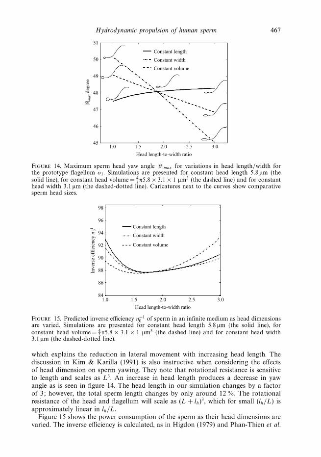
Figure 14. Maximum sperm head yaw angle |θ |max for variations in head length/width forthe prototype flagellum σ1. Simulations are presented for constant head length 5.8 μm (thesolid line), for constant head volume= 4
3π5.8 × 3.1 × 1 μm3 (the dashed line) and for constant
head width 3.1 μm (the dashed-dotted line). Caricatures next to the curves show comparativesperm head sizes.
1.0 1.5 2.0 2.5 3.084
86
88
90
92
94
96
98
Head length-to-width ratio
Inver
se e
ffic
iency
η0–1 Constant length
Constant width
Constant volume
Figure 15. Predicted inverse efficiency η−10 of sperm in an infinite medium as head dimensions
are varied. Simulations are presented for constant head length 5.8 μm (the solid line), forconstant head volume= 4
3π5.8 × 3.1 × 1 μm3 (the dashed line) and for constant head width
3.1 μm (the dashed-dotted line).
which explains the reduction in lateral movement with increasing head length. Thediscussion in Kim & Karilla (1991) is also instructive when considering the effectsof head dimension on sperm yawing. They note that rotational resistance is sensitiveto length and scales as L3. An increase in head length produces a decrease in yawangle as is seen in figure 14. The head length in our simulation changes by a factorof 3; however, the total sperm length changes by only around 12 %. The rotationalresistance of the head and flagellum will scale as (L + lh)
3, which for small (lh/L) isapproximately linear in lh/L.
Figure 15 shows the power consumption of the sperm as their head dimensions arevaried. The inverse efficiency is calculated, as in Higdon (1979) and Phan-Thien et al.

468 E. A. Gillies, R. M. Cannon, R. B. Green and A. A. Pacey
(1987), as
η−10 =
P
6πμAU 2, (4.2)
where A is the volume average radius of the head (Phan-Thien et al. 1987). Althoughthe inverse efficiency curve is quite flat, there are minima in the curves close tothe ‘standard’ sperm head aspect ratio. The observation that the power curves are‘U-shaped’ means that there is a sperm head aspect ratio for maximum efficiency. Inan infinite medium, we predict this maximum efficiency to occur at a head aspectratio of around 1.57 for the constant volume line, 1.7 for the constant width lineand 1.72 for the constant length line of figure 15. These maximum hydrodynamicefficiencies occur at a head dimension range very close to 1.50–1.75 regarded asnormal morphology by WHO (1999).
5. ConclusionsDigital microscopy was used in this paper to obtain the flagellar beat velocity and
head centroid position of several human spermatozoa. The observed kinematics ofthese cells were compared with the predictions of a hydrodynamic method based onthe method of regularized stokeslets. In order to implement the hydrodynamic method,an ellipsoidal head and flagellum were discretized, and chamber walls were alsodiscretized in some simulations. These walled simulations were for a cell swimmingexactly half-way between parallel walls. Power consumption was estimated and wasfound to be higher for simulations where walls were included. However, the kinematicparameters were not largely affected by the presence of walls.
The kinematics and resulting tracks of the sperm, measured at high frame rate, arecomplicated and individual cells can move between square-wave-like and triangular-wave-like or other shaped tracks. These details are reproduced by the hydrodynamicmodel despite the fact that only two dimensions (planar) tail motions were observed.Fine detail in the tracks is also captured in some cases. Transverse velocity andyaw angle were very well captured in all simulations, but average forward propulsivevelocity was underpredicted compared to experiment. Given that the model doesnot underpredict forward propulsive velocity when applied to travelling wave testcases (which do not require numerical differentiation of tail position to infer beatvelocity), it is postulated that the underprediction of forward progressive velocity ofthe experimental cases indicates sensitivity to noise, or missing information, in the taildata. For example, some of the propulsive velocity measured in experiment could havebeen due to intrinsic three-dimensional tail motion of the sperm. Any out-of-planemotions could not be measured in our experiment.
Power consumption calculated for the sperm was very much dependent on whetherslide chamber walls were included in the simulation – for the shallowest chamberswe tested, our power prediction was up to 50 % greater when walls were included.We can conclude that calculations of power expenditure for sperm in MicrocellTM
chambers, or between slide and coverslip, should take chamber walls into account.It is important to understand better the effect of finite chamber depth since currentinternational guidelines for human sperm observation suggest that only chambers ofdepth 20 μm and above may be used during laboratory analysis for clinical purposes.However, we note a moderate increase in power consumption of our simulated spermeven at this chamber depth.

Hydrodynamic propulsion of human sperm 469
Human sperm are pleomorphic, so even sperm with healthy, normal flagella displaya range of head size and shape. For clinical purposes, head dimensions, which areimportant parameters in defining sperm function (WHO 1999), are obtained fromstained images of fixed (dead) sperm. A prototype model of one of the sperm wasused to investigate the effects of head shape on the propulsive velocities for completecycles of flagellar motion. The present fluid mechanical analysis suggests that headdimension is a factor in determining the progressive velocity and amplitude of lateralhead movement and yawing of the sperm (all other aspects of the flagellar motionbeing equal). Narrow heads have the highest forward progressive velocity. Heads withshort lengths have a large lateral movement compared to longer heads. Elongation ofthe sperm head, while keeping the head volume constant, only has a small beneficialeffect on VSL. However, minima in the power consumptions for these simulationswere found where the sperm have ‘normal’ aspect ratio (an aspect ratio between 1.5and 1.75). This suggests that the range of aspect ratios assessed as being ‘normal’also correlates closely with the most efficient hydrodynamic range of aspect ratio.This paper addresses the fluid mechanical effect of these head variations for a fixedflagellar motion, and should therefore be of some use to andrologists by informingthem of the fluid mechanical effects of head dimension on sperm kinematics. In actualsperm populations, however, some head abnormality and variations in head size maybe accompanied by abnormal flagella size or function. This paper does not addresschanges to the flagellar beat that may be associated with abnormalities of the head.We have only studied forward progressive motion here, and it may be that the headhas beneficial hydrodynamic effects for hyperactivated motility.
This work was funded by the Medical Research Council under the DisciplineHopping Scheme (grant G0001205) and Scottish Enterprise under the Proof ofConcept Scheme (project reference 4-BPD007). Richard Cannon was also supportedby the Royal Society of Edinburgh and Scottish Enterprise under the EnterpriseResearch Fellowship initiative. Assistance with the preparation of semen sampleswas provided by Matthew Fletcher and Daniel Smith of the Andrology Laboratory,Sheffield Teaching Hospitals. The authors are grateful to Professor Tim Birkhead(Department of Animal and Plant Sciences, University of Sheffield) for criticalcomments on the draft manuscripts.
Appendix: Details of the data-capture experimentHuman spermatozoa were obtained from patients and donors attending the
Andrology Laboratory located in the Jessop Wing of the Royal Hallamshire Hospital,Sheffield, UK. Procedures were approved by the South Sheffield Research EthicsCommittee (protocol number 04/Q2305/30) and informed consent to make digitalvideo recordings of spermatozoa was obtained from each male donating a specimento this study. For each specimen provided, the sample was collected by masturbationinto a sterile, wide-mouthed container (Sarstedt Ltd, Leicester, UK) following aperiod of 3–5 days sexual abstinence. Following production, each sample was keptat a temperature of 37 ◦C for 30 min before routine procedures of semen analysiswere performed according to World Health Organization (WHO) guidelines (WHO1999). If the specimen was found to be normozoospermic at semen analysis, a highlymotile suspension of spermatozoa was obtained from the remainder of the sample bydensity centrifugation of a 1 ml aliquot of liquefied semen through a Percoll gradient asdescribed by Mortimer (1994). The final concentration of spermatozoa obtained was

470 E. A. Gillies, R. M. Cannon, R. B. Green and A. A. Pacey
(a) (b)
(c) (d)
Figure 16. Sequence of still digital video camera images showing a swimming sperm andmeasured track (the solid black line): (a) start of the track; (b) position and track after0.48 s; (c) position and track after 0.96 s; (d ) position and track after 1.44 s. The other spermin the image is immotile.
adjusted to approximately 20 million sperm per ml in Earle’s Balanced Salt Solution(EBSS) (Sigma Chemical Co., Poole, UK) containing 0.3 % (w/v) human serumalbumin (Sigma Chemical Co., Poole, UK). Sperm preparations were maintained in ahumid atmosphere at 37 ◦C in 5 % CO2 for up to six hours prior to being observed.Samples were placed into MicrocellTM slides (Conception Technologies, San Diego,USA) just prior to inspection by microscope, and cell chamber depths of 12 μm,20 μm and 50 μm were used during the experimentation.
Spermatozoa were observed using a microscope and a digital image capture system.This was based on a Nikon Eclipse E600 upright microscope fitted with phase contrastrings, an (x, y, z) motorized, heated stage and a × 20 objective (numerical aperture0.45). At this magnification, the field of view was approximately 0.05 mm × 0.05 mm,and the depth of field was calculated to be 4 μm. Stage illumination was providedby a lamphouse fitted with a 100-W halogen bulb. For digital video photography,the microscope was equipped with a Dalsa model 2M30 monochrome, 10-bit digitalvideo camera, which has a pixel resolution of 1600 × 1200 pixel and a sensor size of7.4 μm per pixel. The normal framing rate of the camera was 30 Hz, but experimentswere also performed with a framing rate of 121 Hz for which a smaller image area of1600 × 200 pixel was recorded. Microscope stage position control and image capturewere provided by a PC running Windows 2000XP programmed in LabviewTM. Thecamera interface to the computer was provided by a National Instruments PCI-1428Camera LinkTM image acquisition card, and the microscope stage position controlsignals were sent through an RS-232 interface. Camera exposure was set automaticallysuch that the images were not saturated, and a typical exposure time was 1 ms. Imagesequences were saved in uncompressed TIFF format. All image analysis, and indeedall hydrodynamic analysis, was performed on Apple G4 and G5 platforms runningOS X.
A sequence of still images in figure 16 shows the typical raw image data.The centroid of the head was tracked automatically, as was head principalaxis (orientation). Progressive motility was determined using standard parameters,including straight-line velocity VSL, average path velocity VAP and amplitude of

Hydrodynamic propulsion of human sperm 471
(a)s/
L
μm
μm
0 0.2 0.4 0.6 0.8 1.0 1.2 1.4
0.2
0.4
0.6
0.8
(b)
s/L
0 0.2 0.4 0.6 0.8 1.0 1.2 1.4
0.2
0.4
0.6
0.8
Time along track (s)
10
20
30
40
–10
0
10
Figure 17. Contours of position coordinates for the flagellum of the sperm depicted infigure 16: (a) x(s/L, t) coordinate; (b) y(s/L, t) coordinate. This data is used to estimate theflagellar beat velocity.
lateral head movement ALH (Mortimer 1994). The average path is calculated, basedon a 30 Hz data sample, with a 5-point moving average of the X–Y track positions.In all of our images, the flagellum could be discerned as a change in grey level, butsometimes the distal end of the flagellum was indistinct. The flagellum may not beclearly delineated in some images (mainly because of slight out-of-focal plane motionor position), but it is clear enough to determine the flagellum length L at some timepoints. As we assumed the flagellum to be inextensible (which is approximately correctLighthill 1976), we then fixed the tail length in all of the images as L. The proximalend of the tail next to the head was distinct in each image, and a model flagellumwas fitted to each image by the following procedure: from the start point an arc wasdrawn towards the distal end of the flagellum at radius ds (with ds approximatelyL/100), and a new point was placed at the position of maximum grey level on thisarc. This new point corresponds to the flagellum position distance ds from the startpoint. The process is repeated for the second point, and so on until the flagellummodel has a total length L. For some of the images, the unclear termination of theflagellum presented a difficulty. In these cases, the clear points on the flagellum wereused to fit a fourth-order polynomial, which was then extrapolated to total lengthL. Raw manipulation of the images yielded tail lengths that varied ±6 μm becauseof optically unclear regions at the distal end of the tail, or from out-of-focal planemovement, but this procedure rectified this length variation. Our image set (given thesmall depth of field and the fact that most of the flagellum maintained focus in eachframe) indicated that these non-planar flagellum motions were quite small. For oneof our experiments, this automatic tracking and morphology procedure was verifiedby additional manual tracing of the track and tail. A typical set of tail data, gatheredautomatically, is shown in figure 17. An example of a section of the automaticallymeasured centroid track and propulsive velocities, associated with this flagellum data,is shown in figure 18. This figure shows results typical of forward progressive sperm,

472 E. A. Gillies, R. M. Cannon, R. B. Green and A. A. Pacey
0.2 0.4 0.6 0.8 1 1.2 1.4
0.2 0.4 0.6 0.8 1.0 1.2 1.4
0.2 0.4 0.6 0.8 1.0 1.2 1.4–10
–5
0
5
10
15
20
25
30
35
40(a) (b)
(c) (d)
Hea
d a
ngle
θ
–200
–150
–100
–50
0
50
100
UP
x (μ
m s
–1)
UP
y (μ
m s
–1)
–150
–100
–50
0
50
100
Time along track (s)
Time along track (s) Time along track (s)
–50 –40 –30 –20 –10
–10
–5
0
5
10
15
20
25
X track (μm)
Y t
rack
(μ
m)
Figure 18. Typical graphs of kinematic parameters measured for the forward progressivesperm image sequence in figure 16 and flagellum data in figure 17: (a) head angle θ (deg),(b) local (head-aligned) frame propulsive velocity Upx , (c) local (head aligned) lateral velocity
Upy (μm s−1) and (d ) head centroid track.
with a local Upx velocity biased in the forward direction (in this case −x) and amore or less zero average Upy . In the raw images, the sperm head was seen to rotatealternately (broadly about the x axis) and so presented an oscillating width profile tothe microscope. Small variations in observed head length were also seen in the rawimages, indicating that the head pitches out of the x–y plane slightly. These motionsmust result from undetected out-of-plane tail motion. Although the hydrodynamicsimulation was three-dimensional, we could extract only two-dimensional (x–y plane)information from the camera and microscope. The simulation is therefore incapableof reproducing this observed head motion, and we were therefore intrigued as to howthe experimentally recorded tracks would compare to the hydrodynamic simulations.As the head presented a time-varying profile to the camera, an averaging method wasused to approximate head length and width. All of the sperm we measured had lengthand width close to the values published by Brennen & Winet (1977) of 5.8 × 3.1 μmand so, because of the difficulty in obtaining exact head dimensions, we chose thismorphology as the standard head morphology for simulation.
REFERENCES
Ainley, J., Durkin, S., Embid, R., Boindala, P. & Cortez, R. 2008 The method of images forregularized stokeslets. J. Comput. Phys. 227, 4600–4616.

Hydrodynamic propulsion of human sperm 473
Aitken, R. J., Sutton, M., Warner, P. & Richardson, D. W. 1985 Relationship between themovement characteristics of human spermatozoa and their ability to penetrate cervical mucusand zona free hamster oocytes. J. Reprod. Fertil. 73, 441–449.
Birkhead, T. 2000 Promiscuity: An Evolutionary History of Sperm Competition and Sexual Conflict .Faber & Faber.
Blake, J. R. 1971 Infinite models for ciliary propulsion. J. Fluid Mech. 49, 209–222.
Blake, J. R. & Chwang, A. T. 1974 Fundamental singularities of viscous flow. Part 1. The imagesystem in the vicinity of a stationary no-slip boundary. J. Engng Math. 8, 23–29.
Brennen, C. & Winet, H. 1977 Fluid mechanics of propulsion by cilia and flagella. Annu. Rev.Fluid Mech. 9, 339–398.
Brenner, H. 1962 The effects of finite boundaries on the stokes resistance of an arbitrary particle.J. Fluid Mech. 12, 35–48.
Brokaw, C. J. 1970 Bending moments in free-swimming flagella. J. Exp. Biol. 43, 155–169.
Cisneros, L. H., Cortez, R., Dombrowski, C., Goldstein, R. E. & Kessler, J. O. 2007 Fluiddynamics of self-propelled microorganisms, from individuals to concentrated populations.Exper. Fluids 43, 737–753.
Cortez, R. 2001 The method of regularized stokeslets. SIAM J. Sci. Comput. 23 (4), 1204–1225.
Cortez, R., Fauci, L. & Medovikov, A. 2005 The method of regularized stokeslets in threedimensions: analysis, validation, and application to helical swimming. Phys. Fluids 17.
Dresdner, R. D. & Katz, D. F. 1981 Relationships of mammalian sperm motility and morphologyto hydrodynamic aspects of cell function. Biol. Reprod. 25, 920–930.
Dresdner, R. D., Katz, D. F. & Berger, S. A. 1980 The propulsion by large amplitude waves ofuniflagellar micro-organisms of finite length. J. Fluid Mech. 97, 591–621.
Fauci, L. J. & Dillon, R. 2006 Biofluidmechanics of reproduction. Annu. Rev. Fluid Mech. 38,371–394.
Fulford, G. R. & Blake, J. R. 1983 On the motion of a slender body near an interface betweentwo immiscible fluids at low Reynolds numbers. J. Fluid Mech. 127, 203–217.
Gomendio, M., Malo, A. F., Garde, J. & Roldan, E. R. S. 2007 Sperm traits and male fertility innatural populations. Reproduction 134, 19–29.
Gray, J. & Hancock, G. J. 1955 The propulsion of sea-urchin spermatozoa. J. Exp. Biol. 32, 82–814.
Gueron, S. & Liron, N. 1992 Ciliary motion modelling, and dynamic multicilia interactions.Biophysical J. 63, 1045–1058.
Hancock, G. J. 1953 The self-propulsion of microscopic organisms through liquids. Proc. R. Soc.Lond. A 217, 96–121.
Happel, J. & Brenner, H. 1981 Low Reynolds Number Hydrodynamics, 2nd ed. Springer.
Higdon, J. J. L. 1979 A hydrodynamic analysis of flagellar propulsion. J. Fluid Mech. 90, 685–711.
Ishikawa, T., Sekiya, G., Imai, Y. & Yamaguchi, T. 2007 Hydrodynamic interactions between twoswimming bacteria. Biophys. J. 93, 2217–2225.
Johnson, R. E. & Brokaw, C. J. 1979 Flagellar hydrodynamics: a comparison between resistive-force theory and slender-body theory. Biophys. J. 25, 113–127.
Katz, D. F. 1974 On the propulsion of micro-organisms near solid boundaries. J. Fluid Mech. 64,33–49.
Kim, S. & Karilla, J. S. 1991 Microhydrodynamics: Principles and Selected Applications . ButterworthHeinemann.
Larsen, L., Scheike, T., Jensen, T. K., Bonde, J. P., Ernst, E., Hjollund, N. H., Zhou, Y.,
Skakkebaek, N. E. & Giwercman, A. 2000 Computer-assisted semen analysis parameters aspredictors for fertility of men from the general population. Hum. Reprod. 15, 1562–1567.
Lighthill, J. 1976 Flagellar hydrodynamics: the John von Neumann lecture. SIAM Review 18,161–229.
Mortimer, D. 1994 Practical laboratory andrology, chapter 7. In Computer-Aided Sperm Analysis .Oxford University Press.
Owen, D. H. & Katz, D. F. 2005 A review of the physical and chemical properties of human semenand the formulation of a semen simulant. J. Androl. 26 (4), 459–469.
Phan-Thien, N., Tran-Cong, T. & Ramia, M 1987 A boundary-element analysis of flagellarpropulsion. J. Fluid Mech. 184, 533–549.

474 E. A. Gillies, R. M. Cannon, R. B. Green and A. A. Pacey
Ramia, M., Tullock, D. L. & Phan-Thien, N. 1993 The role of hydrodynamic interaction in thelocomotion of microorganisms. Biophys. J. 65, 755–778.
Reynolds, A. J. 1965 The swimming of minute organisms. J. Fluid Mech. 23, 241–260.
Rothschild, Lord 1963 Non-random distribution of bull spermatozoa in a drop of spermsuspension. Nature 198, 1221.
Suarez, S. S. & Pacey, A. A. 2006 Sperm transport in the female reproductive tract. Hum. Reprod.Update 20, 23–37.
Taylor, G. I. 1951 Analysis of the swimming of microscopic organisms. Proc. R. Soc. Lond. A 209,447–461.
WHO 1999 WHO Laboratory Manual for the Examination of Human Semen and Sperm–CervicalMucus Interaction, 4th ed. Cambridge University Press.
Yundt, A. P., Shack, W. J. & Lardner, T. J. 1975 Applicability of hydrodynamic analyses ofspermatozoan motion. J. Exp. Biol. 62, 27–41.